Simplified Procedure for Calculating Exhaust/Intake ... · ASHRAE Transactions 47 uncapped and...

Simplified Procedure for CalculatingExhaust/Intake Separation Distances

Ron L. Petersen, PhD Jared RitterFellow ASHRAE Associate Member ASHRAE

ST-16-005 (RP-1635)

This paper is based on findings resulting from ASHRAE Research Project RP-1635.

ABSTRACT

The purpose of this research project is to provide asimple yet accurate procedure for calculating the minimumdistance required between the outlet of an exhaust systemand the outdoor air intake to a ventilation system to avoidreentrainment of exhaust gases. The new procedureaddresses the technical deficiencies in the simplified equa-tions and tables that are currently in ANSI/ASHRAE Stan-dard 62.1-2016, Ventilation for Acceptable Indoor AirQuality (ASHRAE 2016a), and model building codes. Thisnew procedure makes use of the knowledge provided inChapter45of the2015ASHRAEHandbook—HVACAppli-cations (ASHRAE 2015), and was tested against variousphysical modeling and full-scale studies.

The studydemonstrated that thenewmethod ismoreaccu-rate than the existing Standard 62.1 equation, which under-predicts and overpredicts observed dilution more frequentlythan the new method. In addition, the new method accounts forthe following additional important variables: stack height,wind speed, and “hidden” intake. The new method also hastheoretically justified procedures for addressing heatedexhaust, louvered exhaust, capped heated exhaust, and hori-zontal exhaust that is pointed away from the intake.

INTRODUCTION

ANSI/ASHRAE Standard 62.1-2016 (ASHRAE 2016a)has air intake minimum separation distances specified for vari-ous types of exhaust sources in Table 5.5-1 of the standard.Other codes and standards (e.g., Uniform Mechanical Code[IAPMO 2015a], International Mechanical Code [ICC 2012],

Uniform Plumbing Code [IAPMO 2015b], and ANSI/ASHRAE Standard 62.2 [ASHRAE 2016b]) also specifyminimum separation distances, all of which appear to be rule-of-thumb based with 1 to 3 m (3 to 10 ft) being the magicnumbers for most exhaust types. The separation distances canbe both far too lenient and far too restrictive depending on thetype of exhaust and exhaust and intake configurations.

Both code and Standard 62.1 requirements are overlysimplistic and fail to account for significant variables such asthe exhaust airflow rate, the enhanced mixing caused by highexhaust discharge velocity, the orientation of the discharge, orthe height of the exhaust relative to intake. Standard 62.1includes an Informative Appendix F that outlines a procedureto account for exhaust airflow rate, velocity, and exhaustorientation to achieve target dilution levels. The appendix isnot mandatory but is given as an example of how to use analyt-ical techniques to show that separation distances other thanthose in Table 5.5-1 are acceptable.

The purpose of this research project is to provide a simpleyet accurate procedure for calculating the minimum distancerequired between the outlet of an exhaust system and theoutdoor air intake to a ventilation system to avoid reentrain-ment of exhaust gases. The procedure addresses the technicaldeficiencies in the simplified equations and tables currently inStandard 62.1. This new procedure makes use of the knowl-edge provided in Chapter 45 of the 2015 ASHRAE Hand-book—HVAC Applications (ASHRAE 2015) and variouswind tunnel and full-scale studies discussed herein.

The new methodology is suitable for standard HVACengineering practice and has exhaust outlet velocity, exhaustair volumetric flow rate, exhaust outlet configuration (capped/

46 © 2016 ASHRAE

Ron L. Petersen is the vice president and Jared Ritter is an engineer at CPP, Inc., Fort Collins, CO.

Published in ASHRAE Transactions, Volume 122, Part 2

uncapped and position/orientation relative to intake), desireddilution ratio, and ambient wind speed as independent vari-ables. The current Standard 62.1 Informative Appendix Fmethod includes some of these factors but does not includevariable wind speed, stack height, plume rise effect caused byexhaust velocity, or hidden intake reduction factors. The newmethod discussed herein takes into account all of these vari-ables. The new method also has theoretically justified proce-dures for addressing heated exhaust, louvered exhaust, cappedheated exhaust, and horizontal exhaust that is pointed awayfrom the intake.

The research started out with an objective to develop twonew procedures from existing and new research with thefollowing characteristics:

• Procedure 1. A general procedure suitable for standardHVAC engineering practice that has exhaust outletvelocity, exhaust air volumetric flow rate, exhaust outletconfiguration (capped/uncapped/horizontal/louvered)and position (vertical separation distance), exhaustdirection, desired dilution ratio, hidden intakes (buildingsidewall), and ambient wind speed as independent vari-ables. Other factors, such as location relative to wallsand edge of building, geometry of the exhaust dischargeand inlets, etc., are reduced to fixed assumptions that arereasonable yet somewhat conservative.

• Procedure 2. A regulatory procedure suitable for Stan-dard 62.1, Standard 62.2, and model building codes thathas only exhaust outlet velocity, exhaust air volumetricflow rate, desired dilution ratio, and a simple way toaccount for orientation relative to the inlet as indepen-dent variables. All other variables are reduced to fixedassumptions that are reasonable yet conservative.

In the end, one simple procedure was developed that metthe overall objectives of the study and is appropriate for thefollowing exhaust types:

• Toilet exhaust from rain-capped vents or dome exhaustfans

• Grease and other kitchen fan exhausts• Combustion flues and vents with either forced or natural

draft discharge in horizontal or vertical direction, withand without flue caps (this includes diesel generators)

• Diesel vehicle emissions• Building exhaust at indoor air temperature through lou-

vered or hooded vents• Plumbing vents• Cooling towers

The method does not address laboratory and industrialventilation process exhausts; large, industrial-sized combus-tion flues and stacks; or packaged units that have integralexhaust and intake locations.

A secondary objective of this project is to address dilutiontargets, a necessary parameter for calculating the separation

distance calculation. Accordingly, minimum dilution factorswere reviewed and updated for various types of exhausts asappropriate, especially those with known emissions and healthimpacts such as combustion exhaust. The results of thatresearch are not discussed herein but can be found in theresearch by Petersen et al. (2015). Table 1 provides a summaryof the minimum recommended dilution factors from thatresearch.

The following sections provide a review of the Standard62.1 equation, discussion of databases that were used to testand compare the Standard 62.1 equation and the new equation,development of the new equation, an evaluation of the new andStandard 62.1 equations against observations, and a discus-sion of the new methodology.

EVALUATION OF EXISTING

STANDARD 62.1 EQUATION

The development of the Standard 62.1 equation can befound in Appendix N of the August 1996 Public Review Draftof ASHRAE Standard 62, which will be referred to as 62-1989R (ASHRAE 1996). The equation development beginswith the minimum dilution equation Dmin found in the 1993ASHRAE Handbook—Fundamentals, Chapter 14 (ASHRAE1993) and in the research by Wilson and Lamb (1994):

Table 1. Summary of Recommended

Minimum Dilution Factors

Exhaust Type Minimum Dilution Factor (DF)

Class 1 air exhaust/relief outlet 5




Wood-burning kitchen exhaust 700

General boilers, natural gas andfuel oil, based on NOx

* ppmfactor, p in percent†

* NOx = nitrous oxides (NO and NO2)† If the NOx ppm is 10, p = 10 and DF = 28.

2.8 × p

Garage entry, automobileloading area, or drive-in queue(light-duty gasoline vehicles)

50

Diesel generators, diesel truckloading area or dock, diesel bus

parking/idling area‡

‡ e = 1 – efficiency of the odor filter. For example, if the filter is 80% efficient, e = 0.2and DF = 400.

2000 × e

Cooling tower exhaust(based on chemicals used for

treatment)10

ASHRAE Transactions 47Published in ASHRAE Transactions, Volume 122, Part 2

(1)

(2)

(3)

where

Do = initial jet dilution

Ds = dilution that occurs versus separation distance

s = “stretched string” distance measured along a trajec-tory

UH = wind speed at the roof level

Ve = discharge velocity

Qe = volume flow rate

= factor that relates the nature of discharge outlet; equals 1 for the vertical discharge and 0 for a capped(or downward) discharge

62-1989R states that C1 ranges from 1.6 to 7 and1 rangesfrom 0.0625 to 0.25 (C2 in 62-1989R).

The minimum separation distance is defined as the short-est “stretched string” distance from the closest point of theoutlet opening to the closest point of the outdoor air intakeopening or operable window, skylight, or door opening alonga trajectory as if a string were stretched between them.

To develop the Standard 62.1 equation, Equations 1, 2,and 3 were first rearranged to solve for s (L in the Standard62.1 equation), which results in

(4)

The equation is then simplified by assuming (ASHRAE1996) the following:

• The 1 term is insignificant• Ve = 0 for capped or non-vertical stacks• UH = 2.5 m/s (500 fpm) average wind speed• C1 = 1.7 (on the low end of the range, giving less credit

for dilution due to the discharge velocity, which tends toincrease the separation distance)

• 1 = 0.25 (on the high end of the range, giving maxi-mum credit for dilution due to separation, and tends toreduce separation distance, and is non-conservative)

Using the above assumptions, the Standard 62.1 equationthen results, or

(5)

(6)

where

Qe = exhaust air volume, L/s (cfm)

D = dilution factor for the exhaust type of concern

Ve = exhaust air discharge velocity, m/s (fpm)

Ve is positive when the exhaust is directed away from theoutdoor air intake at a direction that is greater than 45° fromthe direction of a line drawn from the closest exhaust point tothe edge of the intake.

Ve has a negative value when the exhaust is directedtoward the intake bounded by lines drawn from the closestexhaust point the edge of the intake.

Ve is set to 0 for other exhaust air directions regardless ofactual velocity. Ve is also set to 0 for vents from gravity (atmo-spheric) fuel-fired appliances, plumbing vents, and othernonpowered exhausts, or if the exhaust discharge is covered bya cap or other device that dissipates the exhaust airstream.

For hot gas exhausts such as combustion products, aneffective additional 2.5 m/s (500 fpm) upward velocity isadded to the actual discharge velocity if the exhaust stream isaimed directly upward and unimpeded by devices such as fluecaps or louvers.

Equation 4, from which Equations 5 and 6 were devel-oped, has the following problems:

• The equation is only valid for flush vents and does notaccount for stack height or height difference betweenthe stack and the air intake.

• Even though an exit velocity term is included, it doesnot adequately account for high-velocity exhaust sys-tems. The velocity term accounts for the added dilutiondue to a higher exit velocity but does not account for theadditional plume rise.

• The assumed value for the constant C1 (1.7), while con-servative, is not supported by the research. According toWilson and Chui (1994) and ASHRAE (1993, 1997),values of 7 and 13 are more appropriate.

• The assumed value for the constant 1 (0.25) is non-conservative and is not supported by the research.According to Wilson and Chui (1994) and ASHRAE(1993, 1997), values ranging from 0.04 to 0.08 are moreappropriate.

• For vertical stacks, a wind speed higher than 2.5 m/s(500 fpm) may be critical because plume rise willdecrease as wind speed increases, while at low windspeed the plume rise will be very large. For flush ventsand capped stacks, a wind speed lower than 2.5 m/s (500fpm) will most likely be the critical case. Speeds as lowas 1 m/s (200 fpm) can occur a significant fraction of thetime (Perkins 1974).

• Setting Ve equal to a negative number when the exhaustis directed away from the intake, while intuitively cor-rect, cannot be derived from the original equation usedto develop the Standard 62.1 approach.

Dmin Do0.5 Ds

0.5+ 2=

Do 1 C1V e

U H--------- 2

+=

Ds 1s2U H

Qe--------------

=

sQe

1U H---------------

0.5D0.5 1 C1

V e

U H--------- 2

+ 0.5

–=

s 0.04Qe0.5 D0.5

V e

2------– (in metres)=

s 0.09Qe0.5 D0.5

V e

400---------– (in feet)=

48 ASHRAE TransactionsPublished in ASHRAE Transactions, Volume 122, Part 2

To evaluate the Standard 62.1 equation, it needs to be rear-ranged so dilution can be predicted for comparison with thedilution values recorded in the databases discussed the “Dilu-tion Databases” section. The rearranged equation is providedas follows:

(I-P) (7)

(SI) (8)

Overall, this section shows some of the problems with thecurrent 62.1 equation and confirms the need for an improvedequation.

DILUTION DATABASES

In order to evaluate the existing Standard 62.1 equationand New4, existing wind tunnel and full-scale data wereassembled and reviewed. Only those wind tunnel databasesthat meet the criteria outlined in the Environmental ProtectionAgency’s (EPA)Guideline for FluidModeling ofAtmosphericDiffusion (Snyder 1981) were used in this study. Some of theimportant criteria considered are as follows: a boundary-layerwind profile representative of the atmosphere was established,the approach turbulence profile was representative of theatmosphere, and Reynolds number independent flow wasestablished.

For the relevant databases, data were entered into aMicrosoft® Excel spreadsheet in a form that would expeditecomparisons with Standard 62.1 Informative Appendix Fequations and the new method. The following subsectionsdiscuss each database.

Database 1—Wilson and Chui (1994)

The following summarizes the important aspects of thisdatabase:

• 1:500 and 1:2000 scale model tests were conducted• Building Reynolds numbers exceeded 104 to meet the

Reynolds number independence criterion by Snyder(1981)

• A wind power law exponent of 0.25 was established andwind speeds at building heights of 5.9 to 12.1 m/s (1200to 2400 fpm) were set

Eleven model building configurations were tested at sixdifferent exhaust velocity ratios (M = Ve/UH). Exhaust param-eters were a flush circular vent with exhaust density ratio vary-ing from 0.14 to 0.38. Velocity ratios varied from 0.8 to 1.5.Building height to width ratios varied from 1 to 12. Wilson andChui (1994) showed that Equations 1, 2, and 3 with 1 = 0.625and C1 = 7 provided a lower bound to the observed dilutionvalues for several building configurations. This database is notused directly to evaluate the performance of the new equation;

rather, the predicted lower bound using Equations 1, 2, and 3with recommended constants are used as a lower boundprediction for comparison purposes.

Wilson and Chui (1994) show comparisons of predicted(Equations 1, 2, and 3) and observed dilution versus normal-ized distance.

Database 2—Wilson and Lamb (1994)

This is a very unique database in that it is based on a full-scale study that was conducted using tracer gas released fromstacks and exhaust vents on Washington State Universitychemistry laboratory buildings “Fulmer Building” and“Annex Building.”


• Each test took place on a different day between January14 and March 11, 1994.

• Hourly meteorological data (wind speed, wind direc-tion, temperature, and the standard deviation of winddirection flucturations ) were collected from an 8 m(26.25 ft) mast erected on the penthouse roof on theAnnex Building. This represents the tallest point of thetest buildings, which minimizes building wake effects.Wind speeds during the testing period varied from 2.2 to8.1 m/s (440 to 1600 fpm). Crosswind turbulence indi-cated by ranged from 6.5° to 24.8°.

• Tracer gas dilution measurements were carried out byreleasing sulfur hexafluoride (SF6) from the uncappedfume hood exhaust vents and collecting four sequentialhourly average air samples from 44 locations. The dis-tances ranged from s = 5 m (16.4 ft) to s = 270 m(886 ft). Sufficient data were collected to ensure that theminimum dilution could be documented.

• Stack heights ranged from 0 to 3.66 m (0 to 12 ft) andaverage velocity ratios M ranged from 0.83 to 8.3.

Wilson and Lamb (1994) provide figures showing thatEquations 1, 2, and 3 with 1 = 0.04 and C1 = 13 provide alower bound estimate of dilution when compared to observa-tions. This confirms the validity of these equations for flushvents with low plume rise. As with the research by Wilson andChui (1994), this database is not used directly to evaluate theperformance of the new equation; rather the predicted lowerbound using Equations 1, 2, and 3 with the recommendedconstants from this study are used as a second lower boundprediction for comparison purposes.

Database 3—ASHRAE Research Project 805

(Petersen et al. 1997)

This study was initially commissioned in 1997 as anASHRAE research project to determine the influence of archi-tectural screens on exhaust dilution. Wind tunnel experimentswere performed with generic building geometry to generate adatabase of concentrations to document the effects of several

D s 11.1sQe

0.5-------------

V e

400---------+

2

=

D s 25sQe

0.5----------

V e

2------+

2

=


screen wall configurations. Baseline exhaust concentrationsobtained without the presence of a screen wall were alsoincluded in the wind tunnel assessment.


• 1:50 scale model tests were conducted in a boundarylayer wind tunnel with velocity profile power law expo-nent of 0.28

• Building Reynolds number >11,000 to meet Reynoldsnumber independence criterion by Snyder (1981)

• Concentration data for various different exhaust config-urations:• Building measurements of 15.2 × 30.48 × 15.2 m

(50 × 100 × 50 ft) (Hb × W × L)• Stack heights (hs) of 0, 0.3, 0.9, 1.5, 2.1, and 3.7 m

(0, 1, 3, 5, 7, and 12 ft)• Volumetric flow rates of 0.25, 2.4, and 9.4 m3/s

(500, 5000, and 20,000 cfm)• Exhaust velocity ratios (M = Ve /UH) ranging from

~1 to 4• Receptors were placed on rooftop and leeward walls• Wind azimuths of 0°, 45°, and 90°• Reference wind speeds of Uref = 3.7 and 11.1 m/s (728

and 2185 fpm) in the wind tunnel

For this study, data were used only for results obtained inthe wind tunnel for cases with no screen wall on the test build-ing. Only data collected at receptor locations on the test build-ing were used, and no downwind or off-building exhaustconcentrations were considered. Data for multiple stackheights, multiple velocity ratios, and wind azimuths of 0° and45° were considered in this evaluation.

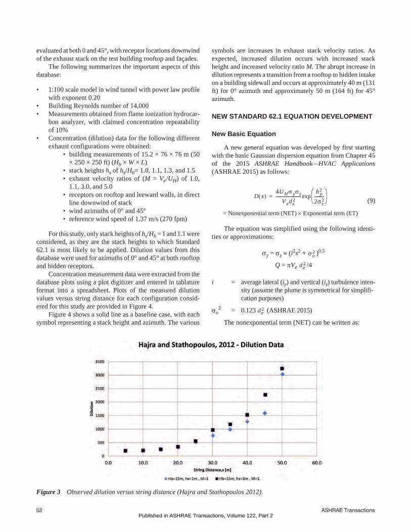
Concentration measurement data from the original windtunnel study were entered in tablature format into a spread-sheet. Plots of the measured dilution values versus stringdistance are provided in Figures 1 and 2 for selected data. Thefigures show a solid line as a baseline case, with each shaderepresenting a fixed volume flow rate and velocity ratio M.The figures show that the observed dilution increases as stackheight is increased for a fixed volume flow rate and velocityratio. The figures also both show the expected trend that asvolume flow rate increases, the dilution decreases for a fixedstack height.

For the 0° orientation, the furthest rooftop receptor loca-tion was located approximately 15 m (49 ft) from the stack.Data taken at distances greater than 15 m (49 ft) indicateconcentrations obtained at a receptor in a “sidewall” location.As expected, a noticeable increase in dilution is observed atsidewall receptor locations.

For the 45° data set, the furthest rooftop receptor locationis located approximately 13 m (42.7 ft) from the stack. Recep-tors at a distance greater than 13 m (42.7 ft) were located onthe leeward wall of the building (sidewall receptors). Asexpected, dilution values were observed to increase at the side-wall intake locations.

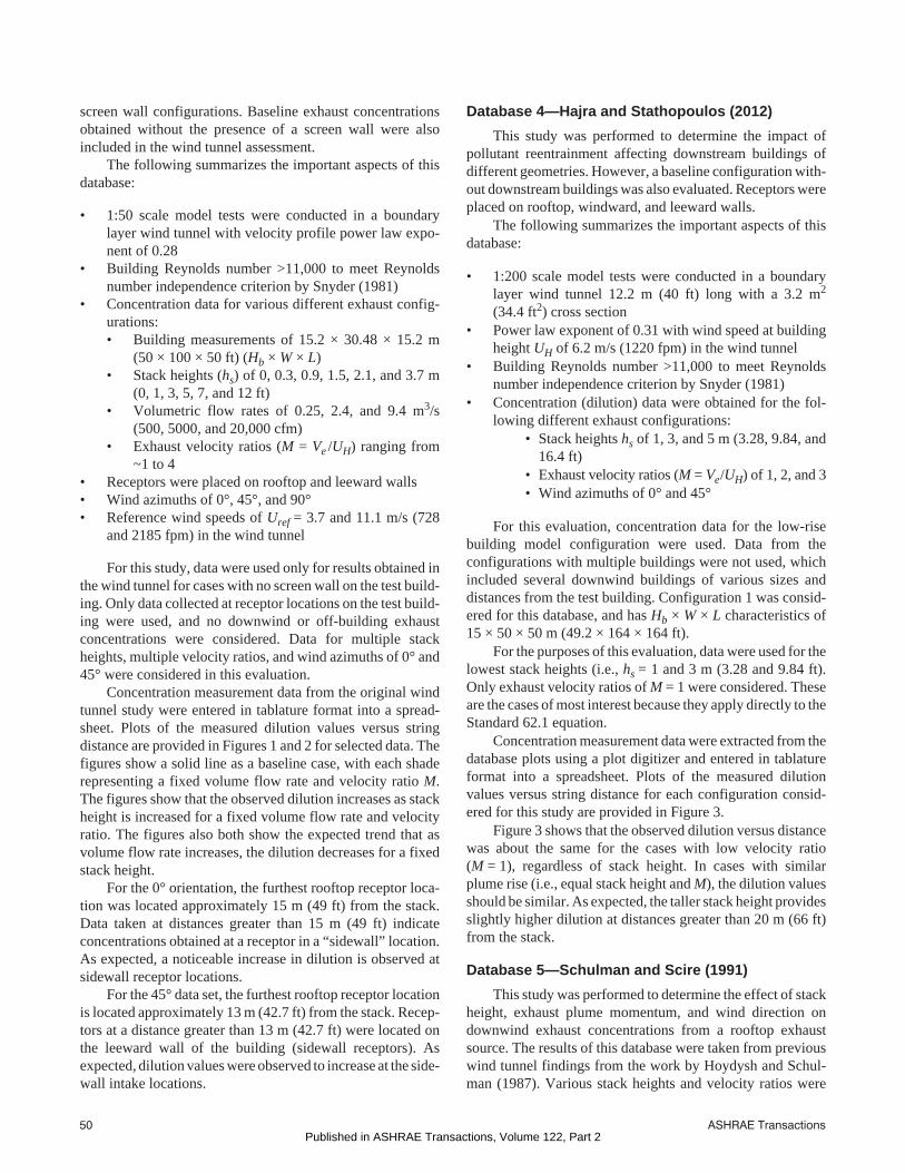
Database 4—Hajra and Stathopoulos (2012)

This study was performed to determine the impact ofpollutant reentrainment affecting downstream buildings ofdifferent geometries. However, a baseline configuration with-out downstream buildings was also evaluated. Receptors wereplaced on rooftop, windward, and leeward walls.


• 1:200 scale model tests were conducted in a boundarylayer wind tunnel 12.2 m (40 ft) long with a 3.2 m2

(34.4 ft2) cross section• Power law exponent of 0.31 with wind speed at building

height UH of 6.2 m/s (1220 fpm) in the wind tunnel• Building Reynolds number >11,000 to meet Reynolds

number independence criterion by Snyder (1981)• Concentration (dilution) data were obtained for the fol-

lowing different exhaust configurations:• Stack heights hs of 1, 3, and 5 m (3.28, 9.84, and

16.4 ft)• Exhaust velocity ratios (M = Ve/UH) of 1, 2, and 3• Wind azimuths of 0° and 45°

For this evaluation, concentration data for the low-risebuilding model configuration were used. Data from theconfigurations with multiple buildings were not used, whichincluded several downwind buildings of various sizes anddistances from the test building. Configuration 1 was consid-ered for this database, and has Hb × W × L characteristics of15 × 50 × 50 m (49.2 × 164 × 164 ft).

For the purposes of this evaluation, data were used for thelowest stack heights (i.e., hs = 1 and 3 m (3.28 and 9.84 ft).Only exhaust velocity ratios of M = 1 were considered. Theseare the cases of most interest because they apply directly to theStandard 62.1 equation.

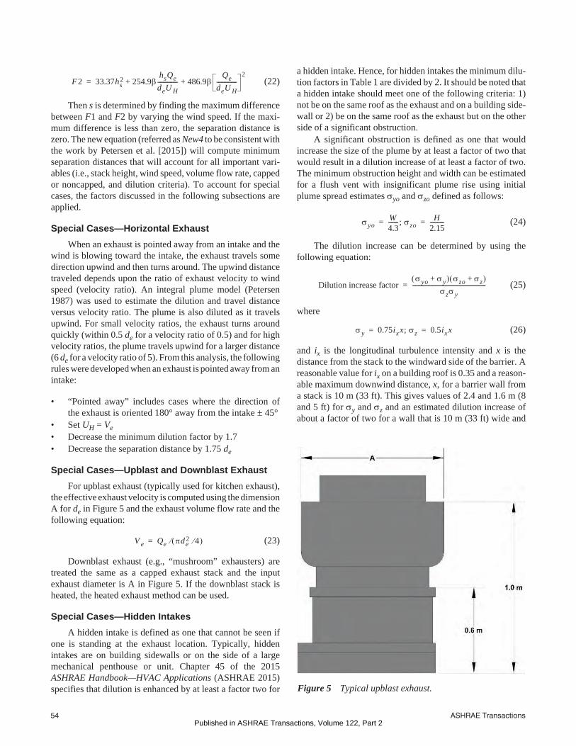
Concentration measurement data were extracted from thedatabase plots using a plot digitizer and entered in tablatureformat into a spreadsheet. Plots of the measured dilutionvalues versus string distance for each configuration consid-ered for this study are provided in Figure 3.

Figure 3 shows that the observed dilution versus distancewas about the same for the cases with low velocity ratio(M = 1), regardless of stack height. In cases with similarplume rise (i.e., equal stack height and M), the dilution valuesshould be similar. As expected, the taller stack height providesslightly higher dilution at distances greater than 20 m (66 ft)from the stack.

Database 5—Schulman and Scire (1991)

This study was performed to determine the effect of stackheight, exhaust plume momentum, and wind direction ondownwind exhaust concentrations from a rooftop exhaustsource. The results of this database were taken from previouswind tunnel findings from the work by Hoydysh and Schul-man (1987). Various stack heights and velocity ratios were


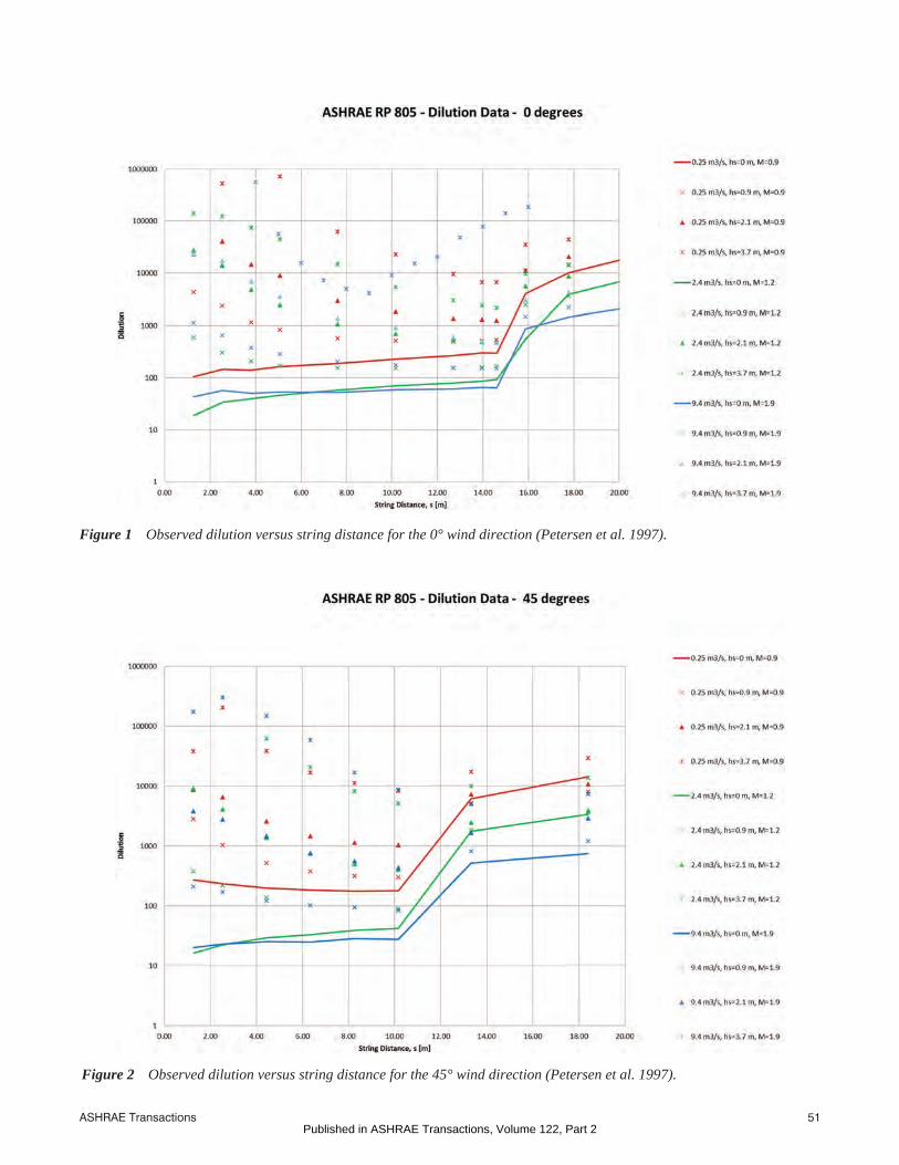
Figure 1 Observed dilution versus string distance for the 0° wind direction (Petersen et al. 1997).

Figure 2 Observed dilution versus string distance for the 45° wind direction (Petersen et al. 1997).


evaluated at both 0 and 45°, with receptor locations downwindof the exhaust stack on the test building rooftop and façades.


• 1:100 scale model in wind tunnel with power law profilewith exponent 0.20

• Building Reynolds number of 14,000• Measurements obtained from flame ionization hydrocar-

bon analyzer, with claimed concentration repeatabilityof 10%

• Concentration (dilution) data for the following differentexhaust configurations were obtained:

• building measurements of 15.2 × 76 × 76 m (50× 250 × 250 ft) (Hb × W × L)

• stack heights hs of hs/Hb= 1.0, 1.1, 1.3, and 1.5• exhaust velocity ratios of (M = Ve/UH) of 1.0,

1.1, 3.0, and 5.0• receptors on rooftop and leeward walls, in direct

line downwind of stack• wind azimuths of 0° and 45°• reference wind speed of 1.37 m/s (270 fpm)

For this study, only stack heights of hs/Hb = 1 and 1.1 wereconsidered, as they are the stack heights to which Standard62.1 is most likely to be applied. Dilution values from thisdatabase were used for azimuths of 0° and 45° at both rooftopand hidden receptors.

Concentration measurement data were extracted from thedatabase plots using a plot digitizer and entered in tablatureformat into a spreadsheet. Plots of the measured dilutionvalues versus string distance for each configuration consid-ered for this study are provided in Figure 4.

Figure 4 shows a solid line as a baseline case, with eachsymbol representing a stack height and azimuth. The various

symbols are increases in exhaust stack velocity ratios. Asexpected, increased dilution occurs with increased stackheight and increased velocity ratio M. The abrupt increase indilution represents a transition from a rooftop to hidden intakeon a building sidewall and occurs at approximately 40 m (131ft) for 0° azimuth and approximately 50 m (164 ft) for 45°azimuth.

NEW STANDARD 62.1 EQUATION DEVELOPMENT

New Basic Equation

A new general equation was developed by first startingwith the basic Gaussian dispersion equation from Chapter 45of the 2015 ASHRAE Handbook—HVAC Applications(ASHRAE 2015) as follows:

(9)

The equation was simplified using the following identi-ties or approximations:

y = z (i2s2 + )0.5

Q = Ve /4

i = average lateral (iy) and vertical (iz) turbulence inten-sity (assume the plume is symmetrical for simplifi-cation purposes)

o2 = 0.123 (ASHRAE 2015)

The nonexponential term (NET) can be written as:

Figure 3 Observed dilution versus string distance (Hajra and Stathopoulos 2012).

D s 4U Hyz

V ede2

-------------------------h p

2

2z2

---------

exp=

= Nonexponential term (NET) Exponential term (ET)

o2

de2

de2


(10)

where

(11)

Now consider the plume rise, ET:

(12)

The plume rise can then be approximated as follows:

(13)

then

(14)

which is still conservative (will underestimate dilution). Anearly approximation to final plume rise (ASHRAE 2007) had = 3.0, which is the value used in this work. The term iz isequal to 0.5 times the longitudinal turbulence intensity, ix,from the work by Snyder (1981). Because i = (iy + iz)/2, which,from the work by Snyder (1981) is equal to (0.75 ix + 0.5 ix)/2, it can be shown that iz = 0.8 i. Substituting into Equation 14results in:

(15)

Expanding:

(16)

where

(17)

Combining the NET and ET terms results in

(18)

This form of the equation was originally evaluated againstthe databases but was found to be too complex for use as a“simple” equation. With the conservative assumption thatB = 0 (no initial dilution due to the size of the release, that is,o is assumed to be small), the equation simplifies to

(19)

which is a form of the quadratic equation from which s can besolved for as follows:

(20)

Substituting and simplifying, the following “new” equa-tion results:

where

(21)

Figure 4 Observed dilution versus string distance (Schulman and Sicre 1991).

NETU Hyz

Qe----------------------

U H

Qe------------ i2s2 0.123de

2+ As2 B+= = =

Ai2U H

Qe-----------------; B

0.385de2U H

Qe-----------------------------= =

ETh p

2

2z2

---------

exp 1h p

2

2z2

--------- 1

2!-----

h p2

2z2

--------- 2

13!-----

h p2

2z2

--------- 3

+ + += =

+ Higher order terms

h p hs h f+ hs deM+=

ET 1hs deM+ 2

2iz2s2

-----------------------------------

+=

ET 1hs 3deM+ 2

2 0.8i 2s2----------------------------------- + 1

hs 3deM+ 2

1.28i2s2----------------------------------- += =

ET 1 11.28i2s2-------------------- hs

2 6hsdeM 9de2M 2+ + +

1 Cs2-----+=

C 11.28i2--------------- hs

2 6hsdeM 9de2M 2+ + =

D s As2 B+ 1 Cs2-----+

As2 B AC BCs2

--------+ + + = =

D As2 AC+=

s2 C– DA----+=

s F1 F2– 0.5=

F1 13.6DQe

U H-----------=


(22)

Then s is determined by finding the maximum differencebetween F1 and F2 by varying the wind speed. If the maxi-mum difference is less than zero, the separation distance iszero. The new equation (referred as New4 to be consistent withthe work by Petersen et al. [2015]) will compute minimumseparation distances that will account for all important vari-ables (i.e., stack height, wind speed, volume flow rate, cappedor noncapped, and dilution criteria). To account for specialcases, the factors discussed in the following subsections areapplied.

Special Cases—Horizontal Exhaust

When an exhaust is pointed away from an intake and thewind is blowing toward the intake, the exhaust travels somedirection upwind and then turns around. The upwind distancetraveled depends upon the ratio of exhaust velocity to windspeed (velocity ratio). An integral plume model (Petersen1987) was used to estimate the dilution and travel distanceversus velocity ratio. The plume is also diluted as it travelsupwind. For small velocity ratios, the exhaust turns aroundquickly (within 0.5 de for a velocity ratio of 0.5) and for highvelocity ratios, the plume travels upwind for a larger distance(6 de for a velocity ratio of 5). From this analysis, the followingrules were developed when an exhaust is pointed away from anintake:

• “Pointed away” includes cases where the direction ofthe exhaust is oriented 180° away from the intake ± 45°

• Set UH = Ve• Decrease the minimum dilution factor by 1.7• Decrease the separation distance by 1.75 de

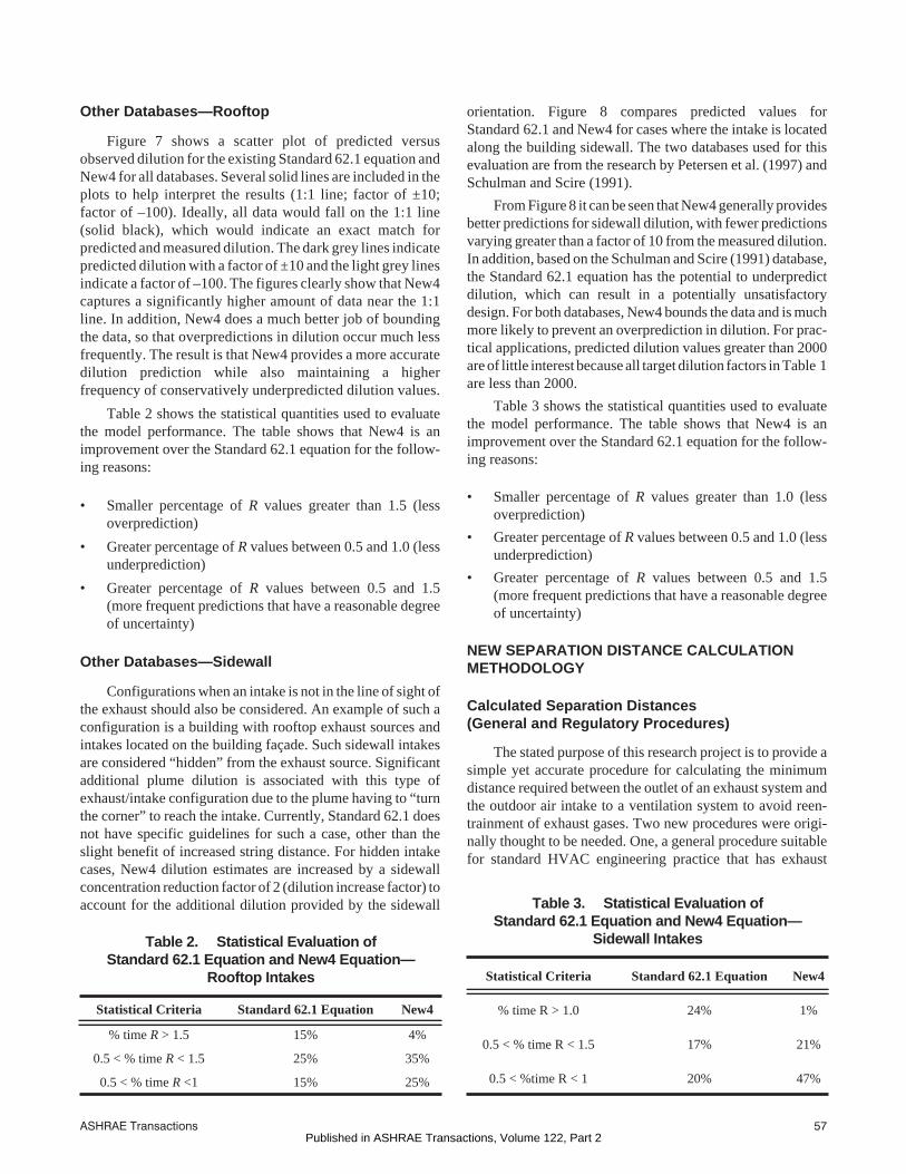
Special Cases—Upblast and Downblast Exhaust

For upblast exhaust (typically used for kitchen exhaust),the effective exhaust velocity is computed using the dimensionA for de in Figure 5 and the exhaust volume flow rate and thefollowing equation:

(23)

Downblast exhaust (e.g., “mushroom” exhausters) aretreated the same as a capped exhaust stack and the inputexhaust diameter is A in Figure 5. If the downblast stack isheated, the heated exhaust method can be used.

Special Cases—Hidden Intakes

A hidden intake is defined as one that cannot be seen ifone is standing at the exhaust location. Typically, hiddenintakes are on building sidewalls or on the side of a largemechanical penthouse or unit. Chapter 45 of the 2015ASHRAE Handbook—HVAC Applications (ASHRAE 2015)specifies that dilution is enhanced by at least a factor two for

a hidden intake. Hence, for hidden intakes the minimum dilu-tion factors in Table 1 are divided by 2. It should be noted thata hidden intake should meet one of the following criteria: 1)not be on the same roof as the exhaust and on a building side-wall or 2) be on the same roof as the exhaust but on the otherside of a significant obstruction.

A significant obstruction is defined as one that wouldincrease the size of the plume by at least a factor of two thatwould result in a dilution increase of at least a factor of two.The minimum obstruction height and width can be estimatedfor a flush vent with insignificant plume rise using initialplume spread estimates yo and zo defined as follows:

(24)

The dilution increase can be determined by using thefollowing equation:

(25)

where

(26)

and ix is the longitudinal turbulence intensity and x is thedistance from the stack to the windward side of the barrier. Areasonable value for ix on a building roof is 0.35 and a reason-able maximum downwind distance, x, for a barrier wall froma stack is 10 m (33 ft). This gives values of 2.4 and 1.6 m (8and 5 ft) for y and z and an estimated dilution increase ofabout a factor of two for a wall that is 10 m (33 ft) wide and

F2 33.37hs2 254.9

hsQe

deU H-------------- 486.9

Qe

deU H--------------

2+ +=

V e Qe de2 4 =

Figure 5 Typical upblast exhaust.

yoW4.3-------; zo

H2.15----------= =

Dilution increase factoryo y+ zo z+

zy----------------------------------------------------=

y 0.75ixx; z 0.5ixx= =


4.6 m (15 ft) high, which equates to a vertical plane squarefootage of 46 m2 (500 ft2). Therefore, a significant obstacle fora flush vent is defined as follows:

• it is located no farther than 10 m (33 ft) from the stack,and

• it has a vertical plane square footage of at least 46 m2

(500 ft2),• it has a height that is greater than one z, or 1.6 m (5.2

ft), which accounts most of the plume above the releasepoint, and

• it has a width that is greater than two y, or 4.8 m (16 ft),which accounts for most of the plume in the lateraldirection.

Alternative larger dilution enhancement factors may bejustified in some cases if additional analysis is carried outusing the method outline above for barriers and as outlined byPetersen et al. (2002, 2004) for building sidewall intakes.Larger downwind distances for the barrier may also be justi-fied using the method outlined above. For taller stacks and/orexhaust with significant plume rise, the required obstacleheight can be estimated using the same method but by addingthe stack height or plume rise to the z value.

Special Cases—Heated Exhaust

New4 assumes plume buoyancy effects are not significantfor plume rise. Therefore, some method needed to be devel-oped to provide some plume rise enhancement for hot exhaust.To develop the method, we started with the following plumerise equation due to momentum and buoyancy (EPA 1995,2004):

(27)

where

(28)

(29)

Because New4 was developed assuming all plume rise isdue to momentum, an equivalent momentum, Mo, equivalent,needs to be computed that gives the same plume rise as thatcaused by momentum and buoyancy effect combined, or

(30)

Expanding and simplifying the following equation can bedeveloped by setting x = 3.05 m (10 ft) and g = 9.8 m/s2

(115,718 ft/min2):

(SI) (31)

(I-P) (32)

where Bfac is the correction factor for heated exhaust. Equa-tions 31 and 32 show Bfac is highest for low winds and low exitvelocities. It tends toward a value of 1 for high wind speedsand high exit velocities.

Special Cases—Capped Heated Exhaust

Capped stacks that are heated will still have plume risebecause of buoyancy effects. To account for this additionalplume rise, a method similar to that recommended by the EPAwill be used. Brode (2015) suggested two alternative methodsfrom which the following method is recommended: multiplydiameter by 10 and maintain the actual volume flow rate,which decreases the exit velocity by a factor of 100. Thismethod results in more reasonable exit velocities (muchgreater than 0.001 m/s [0.2 fpm]) and exhaust diameters thanthe EPA recommended method. For this calculation is setequal to 1. An example calculation is found in the work byPetersen et al. (2015).

EVALUATION OF NEW AND EXISTING

STANDARD 62.1 EQUATIONS

Dilution Equation Performance Metrics

When evaluating models for measurements and predic-tions paired in space and time, such as for this evaluation, thefollowing model performance measures are often used (Hannaet al. 2004):

(33)

(34)

whereFB = fractional biasNMSE = normalized mean-square errorDo = observed dilutionDp = model prediction of dilutionoverbar = average over the date set

These statistics were initially used for the performanceevaluation but were found to provide little useful informationsince a conservative model is desired, or one that will under-predict dilution most of the time with some overpredictionsoccurring. Therefore, more relevant statistics were developed.

h Mo Bo+ 1 3/3T ar2V e

2x

T sU H2

-------------------------- 3g T s T a– r2V ex2

2T aU H3

------------------------------------------------

+1 3/

= =

Mo momentum rise3T r2V e

2x

T sU H2

----------------------- 1 3/

= =

Bo buoyant rise3 T s T a– r2V ex2

2T aU H3

-------------------------------------------- 1 3/

= =

Mo equivalent Mo Bo+ =

Qe b Qe 130.5 T s T a– T s

T a2U H V e

----------------------------------------

+0.5

Qe *B fac= =

Qe b Qe 11180800 T s T a– T s

T a2U H V e

---------------------------------------------------

+0.5

Qe *B fac= =

FB 2Do D p–

DoD p

--------------------=

NMSEDo D p– 2

DoD p

----------------------------=


The ratio R of predicted to observed dilution was computed aswas the percent time that the ratio met the following criteria:

• % time R > 1.5 (percent time dilution predictions are afactor of 1.5 or more high): the best model will have alow percentage.

• % time 0.5 R 1.5 (percent time dilution predictionsare between a factor of 0.5 low to 1.5 high): the bestmodel will have a high percentage.

• % time 0.5 R 1 (percent time dilution predictions arebetween a factor of 0.5 low to perfect agreement): thebest model will have a high percentage.

Another performance measure is a scatter plot ofpredicted divided by observed dilution with a one-to-one line.Again, the ideal model in this case will have almost allpredicted dilution values equal to the observed dilution with afew values greater than observed and most values less thanobserved. The goal is that New4 over- and underpredicts lessthan the current Standard 62.1 equation.

Wilson and Chui (1994) and Wilson and Lamb (1994)

Database Comparison

Actual data from the Wilson and Chui (1994) and Wilsonand Lamb (1994) databases were not obtained, but the equa-tions developed from those databases did bound the measureddata and provide a standard from which to evaluate the Stan-dard 62.1 equation and New4. Figure 6a shows the predictedminimum dilution using the Standard 62.1 equation versus

normalized string distance compared with predictionsobtained using Equations 1, 2, and 3 with Ve / UH (M) = 3.3, perWilson and Lamb (1994), and using the following:

• C1 = 7.0 and 1 = 0.0625 as recommended by Wilsonand Chui (1994 [hereon W&C 94]) and

• C1 = 13.0 and 1 = 0.04 as recommended by Wilson andLamb (1994 [hereon W&L 94]).

These constants were found to bound all observed dilu-tion values in W&C 94 and W&L 94 and should be consideredthe most conservative. Inspection of Figure 6a shows that allminimum dilution equations (except Standard 62.1) producesimilar results for normalized distances () greater than about20, while the Standard 62.1 and W&C 94 equations providedthe lowest dilution estimates for < ~10.

New4 was then tested against the W&C 94 and W&L94 equations and an i value of 0.153 was determined to providea best fit with W&C 94 for 20 < < 1000. Figure 6a showsNew4 dilution equation estimates versus those obtained usingW&C94andW&L94with thegraph fromW&L94on the right(Figure 6b), which includes the measured data. The solid line inFigure 6b corresponds with the W&L 94 line in Figure 6a. Bycomparing the two figures it canbe seen thatNew4doesprovidea lower bound for the observed dilution values for normalizeddistance > 20 and also shows that dilution is approximatelyconstant closer to the stack. This is the effect of the plume rise,which is not included in the Standard 62.1 equation. For < 10,New4 approximately bounds the limited observations.

(a) (b)

Figure 6 Comparison of predicted dilution using the Standard 62.1, Wilson and Lamb (1994), Wilson and Chui (1994), andNew4.


Other Databases—Rooftop

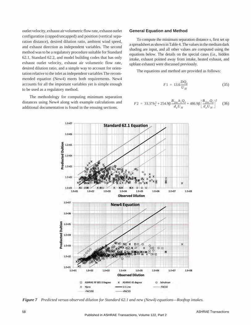
Figure 7 shows a scatter plot of predicted versusobserved dilution for the existing Standard 62.1 equation andNew4 for all databases. Several solid lines are included in theplots to help interpret the results (1:1 line; factor of ±10;factor of –100). Ideally, all data would fall on the 1:1 line(solid black), which would indicate an exact match forpredicted and measured dilution. The dark grey lines indicatepredicted dilution with a factor of ±10 and the light grey linesindicate a factor of –100. The figures clearly show that New4captures a significantly higher amount of data near the 1:1line. In addition, New4 does a much better job of boundingthe data, so that overpredictions in dilution occur much lessfrequently. The result is that New4 provides a more accuratedilution prediction while also maintaining a higherfrequency of conservatively underpredicted dilution values.

Table 2 shows the statistical quantities used to evaluatethe model performance. The table shows that New4 is animprovement over the Standard 62.1 equation for the follow-ing reasons:

• Smaller percentage of R values greater than 1.5 (lessoverprediction)

• Greater percentage of R values between 0.5 and 1.0 (lessunderprediction)

• Greater percentage of R values between 0.5 and 1.5(more frequent predictions that have a reasonable degreeof uncertainty)

Other Databases—Sidewall

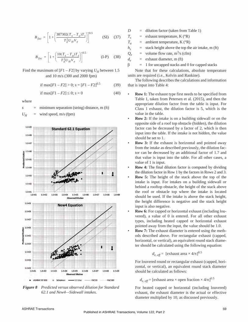
Configurations when an intake is not in the line of sight ofthe exhaust should also be considered. An example of such aconfiguration is a building with rooftop exhaust sources andintakes located on the building façade. Such sidewall intakesare considered “hidden” from the exhaust source. Significantadditional plume dilution is associated with this type ofexhaust/intake configuration due to the plume having to “turnthe corner” to reach the intake. Currently, Standard 62.1 doesnot have specific guidelines for such a case, other than theslight benefit of increased string distance. For hidden intakecases, New4 dilution estimates are increased by a sidewallconcentration reduction factor of 2 (dilution increase factor) toaccount for the additional dilution provided by the sidewall

orientation. Figure 8 compares predicted values forStandard 62.1 and New4 for cases where the intake is locatedalong the building sidewall. The two databases used for thisevaluation are from the research by Petersen et al. (1997) andSchulman and Scire (1991).

From Figure 8 it can be seen that New4 generally providesbetter predictions for sidewall dilution, with fewer predictionsvarying greater than a factor of 10 from the measured dilution.In addition, based on the Schulman and Scire (1991) database,the Standard 62.1 equation has the potential to underpredictdilution, which can result in a potentially unsatisfactorydesign. For both databases, New4 bounds the data and is muchmore likely to prevent an overprediction in dilution. For prac-tical applications, predicted dilution values greater than 2000are of little interest because all target dilution factors in Table 1are less than 2000.

Table 3 shows the statistical quantities used to evaluatethe model performance. The table shows that New4 is animprovement over the Standard 62.1 equation for the follow-ing reasons:

• Smaller percentage of R values greater than 1.0 (lessoverprediction)

• Greater percentage of R values between 0.5 and 1.0 (lessunderprediction)

• Greater percentage of R values between 0.5 and 1.5(more frequent predictions that have a reasonable degreeof uncertainty)

NEW SEPARATION DISTANCE CALCULATION

METHODOLOGY

Calculated Separation Distances

(General and Regulatory Procedures)

The stated purpose of this research project is to provide asimple yet accurate procedure for calculating the minimumdistance required between the outlet of an exhaust system andthe outdoor air intake to a ventilation system to avoid reen-trainment of exhaust gases. Two new procedures were origi-nally thought to be needed. One, a general procedure suitablefor standard HVAC engineering practice that has exhaust

Table 2. Statistical Evaluation of

Standard 62.1 Equation and New4 Equation—

Rooftop Intakes

Statistical Criteria Standard 62.1 Equation New4

% time R > 1.5 15% 4%

0.5 < % time R < 1.5 25% 35%

0.5 < % time R <1 15% 25%

Table 3. Statistical Evaluation of

Standard 62.1 Equation and New4 Equation—

Sidewall Intakes

Statistical Criteria Standard 62.1 Equation New4

% time R > 1.0 24% 1%

0.5 < % time R < 1.5 17% 21%

0.5 < %time R < 1 20% 47%


outlet velocity, exhaust air volumetric flow rate, exhaust outletconfiguration (capped/uncapped) and position (vertical sepa-ration distance), desired dilution ratio, ambient wind speed,and exhaust direction as independent variables. The secondmethod was to be a regulatory procedure suitable for Standard62.1, Standard 62.2, and model building codes that has onlyexhaust outlet velocity, exhaust air volumetric flow rate,desired dilution ratio, and a simple way to account for orien-tation relative to the inlet as independent variables The recom-mended equation (New4) meets both requirements. New4accounts for all the important variables yet is simple enoughto be used as a regulatory method.

The methodology for computing minimum separationdistances using New4 along with example calculations andadditional documentation is found in the ensuing sections.

General Equation and Method

To compute the minimum separation distance s, first set upa spreadsheet as shown inTable4.Thevalues in themediumdarkshading are input, and all other values are computed using theequations below. The details on the special cases (i.e., hiddenintake, exhaust pointed away from intake, heated exhaust, andupblast exhaust) were discussed previously.

The equations and method are provided as follows:

(35)

(36)

Figure 7 Predicted versus observed dilution for Standard 62.1 and new (New4) equations—Rooftop intakes.

F1 13.6DQe

U H-----------=

F2 33.37hs2 254.9

B fachsQe

deU H----------------------- 486.9

B facQe

deU H------------------

2+ +=


(SI) (37)

(I-P) (38)

Find the maximum of [F1 – F2] by varying UH between 1.5and 10 m/s (300 and 2000 fpm)

if max[F1 – F2] > 0; s = [F1 – F2]0.5 (39)

if max[F1 – F2] 0; s = 0 (40)

where

s = minimum separation (string) distance, m (ft)

UH = wind speed, m/s (fpm)

D = dilution factor (taken from Table 1)Ts = exhaust temperature, K (°R)Ta = ambient temperature, K (°R)hs = stack height above the top the air intake, m (ft)Qe = volume flow rate, m3/s (cfm)de = exhaust diameter, m (ft) = 1 for uncapped stacks and 0 for capped stacks

Note that for these calculations, absolute temperatureunits are required (i.e., Kelvin and Rankine).

The following describes the calculations and informationthat is input into Table 4:

• Row 1: The exhaust type first needs to be specified fromTable 1, taken from Petersen et al. (2015), and then theappropriate dilution factor from the table is input. ForClass 1 exhaust, the dilution factor is 5, which is thevalue in the table.

• Row 2: If the intake is on a building sidewall or on theopposite side of a roof top obstacle (hidden), the dilutionfactor can be decreased by a factor of 2, which is theninput into the table. If the intake is not hidden, the valueshould be set to 1.

• Row 3: If the exhaust is horizontal and pointed awayfrom the intake as described previously, the dilution fac-tor can be decreased by an additional factor of 1.7 andthat value is input into the table. For all other cases, avalue of 1 is input.

• Row 4: The final dilution factor is computed by dividingthe dilution factor in Row 1 by the factors in Rows 2 and 3.

• Row 5: The height of the stack above the top of theintake is input. For intakes on a building sidewall orbehind a rooftop obstacle, the height of the stack abovethe roof or obstacle top where the intake is locatedshould be used. If the intake is above the stack height,the height difference is negative and the stack heightinput is also negative.

• Row 6: For capped or horizontal exhaust (including lou-vered), a value of 0 is entered. For all other exhausttypes, including heated capped or horizontal exhaustpointed away from the input, the value should be 1.0.

• Row 7: The exhaust diameter is entered using the meth-ods described above. For rectangular exhaust (capped,horizontal, or vertical), an equivalent round stack diame-ter should be calculated using the following equation:

de, eff = [exhaust area × 4/]0.5

For louvered round or rectangular exhaust (capped, hori-zontal, or vertical), an equivalent round stack diametershould be calculated as follows:

de, eff = [exhaust area × open fraction × 4/]0.5

For heated capped or horizontal (including louvered)exhaust, the exhaust diameter is the actual or effectivediameter multiplied by 10, as discussed previously.

Figure 8 Predicted versus observed dilution for Standard62.1 and New4—Sidewall intakes.

B fac 1387302 T s T a– T s

T a2U H V e

------------------------------------------------

+0.5

=

B fac 110 T s T a– T s

T a2U H V e

------------------------------------

+0.5

=


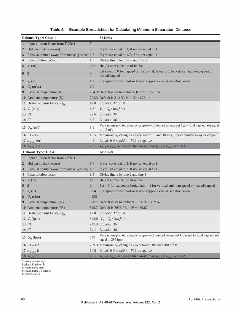
Table 4. Example Spreadsheet for Calculating Minimum Separation Distance

Exhaust Type: Class 1 SI Units

1 Input dilution factor from Table 1 5

2 Hidden intake (yes/no) 2 If yes, set equal to 2; if no, set equal to 1

3 Exhaust pointed away from intake (yes/no) 1.7 If yes, set equal to 1.7; if no, set equal to 1

4 Final dilution factor 1.5 Divide line 1 by row 2 and row 3

5 hs (m) 0.31 Height above the top of intake

6 0Set equal to 0 for capped or horizontal; equal to 1 for vertical and noncapped orheated/capped

7 de (m) 1.2 For upblast/downblast or heated capped exhaust, see discussion

8 Qe (m3/s) 2.0

9 Exhaust temperature (K) 294.3 Default is set to ambient, K = °C + 273.14

10 Ambient temperature (K) 294.3 Default is 21.1°C, K = °C + 273.14

11 Heated exhaust factor, Bfac 1.00 Equation 37 or 38

12 Ve (m/s) 1.8 Ve = Qe / ( /4)

13 F1 22.6 Equation 35


15 UH (m/s) 1.8Vary unless pointed away or capped—If pointed, always set UH = Ve; if capped, set equalto 1.5 m/s

16 F1 – F2 19.5 Maximize by changing UH between 1.5 and 10 m/s, unless pointed away or capped

17 sinitial (m) 4.4 Equals 0 if max[F1 – F2] is negative

18 sfinal (m) 2.3 sfinal = sinitial unless pointed away; then sfinal = sinitial – 1.75de

Exhaust Type: Class 1 I-P Units

1 Input dilution factor from Table 1 5

2 Hidden intake (yes/no) 1.0 If yes, set equal to 2. If no, set equal to 1.

3 Exhaust pointed away from intake (yes/no) 1.7 If yes, set equal to 2. If no, set equal to 1.

4 Final dilution factor 1.5 Divide line 1 by line 2 and line 3

5 hs (ft) 1.0 Height above the top of intake

6 0 Set = 0 for capped or horizontal, = 1 for vertical and noncapped or heated/capped

7 de (ft) 3.94 For upblast/downblast or heated capped exhaust, see discussion

8 Qe (cfm) 4235

9 Exhaust temperature (°R) 529.7 Default is set to ambient, °R = °F + 459.67

10 Ambient temperature (°R) 529.7 Default is 70°F, °R = °F + 459.67

11 Heated exhaust factor, Bfac 1.00 Equation 37 or 38

12 Ve (fpm) 348.0 Ve = Qe / ( /4)

13 F1 243.3 Equation 35


15 UH (fpm) 348Vary unless pointed away or capped—If pointed, aways set UH equal to Ve; if capped, setequal to 295 fpm

16 F1 – F2 209.3 Maximize by changing UH between 300 and 2000 fpm

17 sinitial, ft 14.5 Equals 0 if max[F1 – F2] is negative

18 sfinal, ft 7.6 sfinal = sinitial unless pointed away; then sfinal = sinitial – 1.75de

Shade gradation key:Darkest: Final resultMedium dark: InputMedium light: CalculationLightest: Varies

de2

de2


• Row 8: The exhaust volume flow rate is entered. Forgravity vents, such as plumbing vents, use an exhaustrate of 75 L/s (150 cfm). For flue vents from fuel-burn-ing appliances, assume a value of 0.43 L/s per kW(250 cfm per million Btu/h) of combustion input (orobtain actual rates from the combustion appliance man-ufacturer).

• Row 9: The exhaust temperature is entered. Unless theexhaust is heated, this temperature should be the sameas the ambient temperature.

• Row 10: Enter the ambient temperature. Default valuesof 294.3 K (21.1°C) or 529.7°R (70°F) should typicallybe used.

• Row 11: The heated exhaust factor is computed usingEquations 37 or 38.

• Row 12: The exhaust velocity is computed using theequation in the table.

• Row 13: F1 is computed using Equation 35.• Row 14: F2 is computed using Equation 36.• Row 15: For noncapped or heated horizontal exhaust

and heated capped exhaust, the wind speed is variedbetween 1.5 and 10 m/s (300 and 2000 fpm) and the dif-ference between F1 and F2 is maximized. If the maxi-mum value is negative, the minimum separationdistance is zero. If the difference is positive, then the ini-tial separation distance is computed using Equation 39.For capped stacks or horizontal exhaust not pointedaway from the intake, a wind speed of 1.5 m/s (300 fpm)should be used. For horizontal exhaust pointed awayfrom the intake, the wind speed should be set equal tothe exit velocity.

• Row 16: F1 – F2 is computed.• Row 17: sinitial is computed using Equations 39 or 40.• Row 18: sfinal is the same as sinitial for all exhaust except

horizontal exhaust that is pointed away. For the lattercase, sfinal is computed using the equation in the table.

CONCLUSIONS

The purpose of this research project was to provide a rela-tively simple yet accurate procedure for calculating the mini-mum distance required between the outlet of an exhaustsystem and the outdoor air intake to a ventilation system toavoid reentrainment of exhaust gases. Accordingly, a newprocedure was developed that addresses the technical defi-ciencies in the simplified equations and tables that arecurrently in ANSI/ASHRAE Standard 62.1 (ASHRAE2016a). The new procedure makes use of the knowledgeprovided in Chapter 45 of the 2015 ASHRAE Handbook—HVAC Applications (ASHRAE 2015) and various wind tunneland full-scale studies discussed herein.

The updated methodology is suitable for standard HVACengineering practice, and for regulatory use suitable forASHRAE Standard 62.1, ASHRAE Standard 62.2, and modelbuilding codes. The new method has exhaust diameter (veloc-ity), exhaust air volumetric flow rate, exhaust outlet configu-

ration (capped/uncapped), position relative to intakeorientation and position (horizontal and pointed away),desired dilution ratio, ambient wind speed, temperature of theexhaust, and hidden versus visible intakes as independent vari-ables.

The updated method was tested against several databases(field and wind tunnel), which demonstrated that the newmethod is more accurate than the existing Standard 62.1 equa-tion in that it underpredicts and overpredicts observed dilutionless frequently. In addition, the new method accounts for thefollowing additional important variables: stack height, windspeed, and hidden versus visible intakes. The new method alsohas theoretically justified procedures for addressing heatedexhaust, louvered exhaust, capped heated exhaust, and hori-zontal exhaust that is pointed away from the intake.

ACKNOWLEDGMENTS

This research was sponsored by ASHRAE TechnicalCommittee 4.3.

REFERENCES

ASHRAE. 1993. Chapter 14 in ASHRAE handbook—Funda-mentals. Atlanta: ASHRAE.

ASHRAE. 1996. ASHRAE Standard 62-1989R. Ventilationfor acceptable indoor air quality—Public review draft.Atlanta: ASHRAE.

ASHRAE. 1997. Chapter 15 in ASHRAE handbook—Funda-mentals. Atlanta: ASHRAE.

ASHRAE. 2015. Chapter 45 in ASHRAE handbook—HVACapplications. Atlanta: ASHRAE.

ASHRAE. 2016a. ANSI/ASHRAE Standard 62.1-2016,Ventilation for acceptable indoor air quality. Atlanta:ASHRAE

ASHRAE. 2016b. ANSI/ASHRAE Standard 62.2-2016,Ventilation and acceptable indoor air quality in low-riseresidential buildings. Atlanta: ASHRAE.

Brode, R.W. 2015. Proposed updates to AERMOD modelingsystem. 11th Modeling Conference Presentation, ResearchTriangle Park, NC. www.epa.gov/ttn/scram/11thmodconf/presentations/1-5_Proposed_Updates_AERMOD_System.pdf.

EPA. 1995. User’s guide for the Industrial Source Complex(ISC3) dispersion models, vol. 2: Description of modelalgorithms. EPA-454/B-95993B. Research TrianglePark, NC: U.S. Environmental Protection Agency.

EPA. 2004. AERMOD, Description of model formulation.EPA-454/R-03-004. Research Triangle Park, NC: U.S.Environmental Protection Agency.

Hajra, B., and T. Stathopoulos. 2012. A wind tunnel study ofthe effect of downstream buildings on near-field pollut-ant dispersion. Building and Environment 52:19–31.

Hanna, S.R., O.R. Hansen, and S. Dharmavaram. 2004.FLACS CFD air quality model performance evaluationwith Kit Fox, MUST, Prairie Grass, and EMU observa-tions. Atmospheric Environment 38:4675–87.


Hoydysh, W.G., and L.L. Schulman. 1987. Fluid modelingstudy of the contamination of fresh air intakes fromrooftop emissions. Paper 87-82A.9, 80th Annual Meet-ing of APCA, New York, NY.

IAPMO. 2015a. Uniform mechanical code. Ontario, Canada:International Association of Plumbing and MechanicalOfficials.

IAPMO. 2015b. Uniform plumbing code. Ontario, Canada:International Association of Plumbing and MechanicalOfficials.

ICC. 2012. International mechanical code. Country ClubHills, IL: International Code Council.

Perkins, H.C. 1974. Air pollution. New York: McGraw-HillBook Company. p. 152.

Petersen, R.L. 1987. Performance evaluation of integral andanalytical plume rise algorithms. Journal of the Air Pol-lution Control Association 37(11):1314–19.

Petersen, R.L., J.J. Carter, and M.A. Ratcliff. 1997. Theinfluence of architectural screens on exhaust dilution.Final Report, ASHRAE 805-TRP. Atlanta: ASHRAE.

Petersen, R.L., B.C. Cochran, and J.J. Carter. 2002. Specify-ing exhaust and intake systems. ASHRAE Journal44(8):30–5.

Petersen, R.L., J.J. Carter, and J.W. LeCompte. 2004.Exhaust contamination of hidden vs. visible air intakes.ASHRAE Transactions 110(1):130–42.

Petersen, R.L, J.D. Ritter, A.S. Bova, and J.J. Carter. 2015Simplified procedure for calculating exhaust/intake sep-aration distances. Final Report, ASHRAE RP 1635-TRP.

Schulman, L.L, and J.S. Scire. 1991. The effect of stackheight, exhaust speed, and wind direction on concentra-tions from a rooftop stack. ASHRAE Transactions 97(2):573–85.

Snyder, W.H. 1981. Guideline for fluid modeling of atmo-spheric diffusion. Report No. EPA600/8–81–009.Research Triangle Park, NC: U.S. Environmental Pro-tection Agency, Environmental Sciences Research Lab-oratory, Office of Research and Development.

Wilson, D.J., and B.K. Lamb. 1994. Dispersion of exhaustgases from roof-level stacks and vents on laboratorybuilding. Atmospheric Environment 28(19):3099–111.

Wilson, D.J., and E.H. Chui. 1994. Influence of building sizeon rooftop dispersion of exhaust gas. Atmospheric Envi-ronment 28(14):2325–34.


Simplified Procedure for Calculating Exhaust/Intake ... · ASHRAE Transactions 47 uncapped and...

Documents

Transcript of Simplified Procedure for Calculating Exhaust/Intake ... · ASHRAE Transactions 47 uncapped and...