Simplified probabilistic slope stability design charts for ... draft.pdf · Slope stability charts...

Original author submission

S. Javankhoshdel and R.J. Bathurst (2014)

of 36

For final and corrected published version see:

Javankhoshdel, S. and Bathurst, R.J. 2014. Simplified probabilistic slope stability

design charts for cohesive and c-ø soils. Canadian Geotechnical Journal 51(9): 1033-

1045 (http://dx.doi.org/10.1139/cgj-2013-0385).

Simplified probabilistic slope stability design charts for

cohesive and c- soils

Sina Javankhoshdel1

Richard J. Bathurst2

1 PhD candidate

GeoEngineering Centre at Queen’s-RMC

Department of Civil Engineering

Ellis Hall

Queens University

Kingston, Ontario, K7L 3N6 CANADA

Phone: (613) 541-6000 (ext. 6347)

Email: [email protected]

2 Professor and Research Director (corresponding author)

GeoEngineering Centre at Queen’s-RMC

Department of Civil Engineering, 13 General Crerar, Sawyer Building, Room 2414,

Royal Military College of Canada, Kingston, Ontario, K7K 7B4 CANADA

Phone: (613) 541-6000 (ext. 6479/6347/6391)

Email: [email protected]

http://dx.doi.org/10.1139/cgj-2013-0385



of 36

ABSTRACT

Design charts to estimate the factor of safety for simple slopes with c- soils are now available in

the literature. However, factor of safety is an imperfect measure to quantify the margin of safety of

a slope because nominal identical slopes with the same factor of safety can have different

probabilities of failure due to variability in soil properties. In this study, simple circular slip slope

stability charts for = 0 soils by Taylor (1937) and c- soils published by Steward et al. (2011)

are extended to match estimates of factor of safety to corresponding probabilities of failure. A series

of new charts are provided that consider a practical range of coefficient of variation (COV) for

cohesive and frictional strength parameters of the soil. The data to generate the new charts were

produced using conventional probabilistic concepts together with closed-form solutions for

cohesive soil cases and Monte Carlo simulation in combination with conventional limit

equilibrium-based circular slip analyses using the program SVSlope for c- soil cases. The charts

are a useful tool for geotechnical engineers to make a preliminary estimate of the probability of

failure of a simple slope without running Monte Carlo simulations.

Keywords: Slope stability; Probabilistic analysis; Monte Carlo simulation; Design chart; Spatial

variability

1 INTRODUCTION

Slope stability charts are used routinely to estimate the factor of safety of slopes with isotropic,

homogeneous soil properties and simple geometry. Taylor (1937) published design charts to

calculate the factor of safety for simple homogeneous slopes in clays with single-value undrained

shear strength. These charts are found in various forms in geotechnical engineering text books. In

the same publication (1937), Taylor presented charts to compute the factor of safety for simple

slopes with cohesive-frictional (c-) shear strength soils. These charts have the disadvantage that

they require an iterative procedure to determine the factor of safety. Since Taylor’s work, other

researchers have developed slope stability charts for simple slopes with c- soils. Michalowski

(2002) used a kinematic approach of limit analysis with a log-spiral failure mechanism while Baker

(2003) and Steward et al. (2011) used conventional limit equilibrium circular slip analyses to

produce their charts. All of these methods are deterministic and the resulting charts can be shown to



of 36

give the same factor of safety for the same slope and soil properties. The advantage of the work by

Steward et al. (2011) is that they produced a single chart for c- soils which does not require an

iterative approach to calculate the factor of safety.

A shortcoming of all these design charts is that an appreciation of the probability of failure of the

slope cannot be made. For example, if the soil properties are treated as random variables then it is

possible that two slopes with nominally identical soil properties and the same slope geometry can

have different probabilities of failure because of differences in variability of the soil properties. In

fact, the assessment of probability of slope failure is further complicated because soil properties

also have spatial variability.

The influence of the random variability of soil strength parameters on probability of failure of

slopes using conventional limit equilibrium slip circle analysis has been explored by Li and Lumb

(1987), Chowdhury and Xu (1993), Low et al. (1998) and Hong and Roh (2008). These

researchers considered slopes having one or more isotropic, homogeneous soil layers with random

strength values described by a single cumulative distribution function. The influence of spatial

variability of soil properties on probability of failure using conventional limit equilibrium slope

stability analyses has also been investigated by Christian et al. (1994), El-Ramly et al. (2002),

Low et al. (2007), Cho (2010) and Wang et al. (2010). Important contributions to the influence of

spatial variability of soil properties on stability of slopes have been made by Griffiths and Fenton

(2004), Griffiths et al. (2009) and Huang et al. (2010) using the random finite element method

(RFEM). All of the above prior work has improved understanding of the quantitative and

qualitative influence of the random and spatial distribution of soil strength properties on the margin

of safety of slopes in probabilistic terms. However, production of design charts for the estimate of

probability of failure of simple slopes with c- soils and conventional slip circle geometry has not

been attempted.

The primary objective of the current study was to develop a series of design charts for simple slopes

that combine quantitative estimates of the conventional factor of safety with matching estimates of

the probability of failure considering random values of cohesive and frictional shear strength

components having lognormal distributions. Two series of design charts are presented.



of 36

The first chart is an extension to the Taylor’s chart for purely cohesive soil cases (i.e. undrained

shear strength parameters = u = 0, c = su and total unit weight ). The resulting design chart is

equivalent to a chart published by Griffiths and Fenton (2004) for the case of variability in

undrained shear strength only. The current study compliments this earlier work by including a

useful closed-form expression for calculation of probability of failure for slopes with random values

of undrained shear strength and unit weight.

The second series of design charts are for c- soils. They were developed from results of Monte

Carlo simulation using the probabilistic circular slip slope stability analysis option in the

commercially available SVSlope software package (Fredlund and Thode 2011). Together, the two

series of charts cover soil slope cases with cohesive and cohesive-frictional soils. Thus this paper

provides a convenient single reference for geotechnical engineers to make estimates of the

conventional factor of safety and probability of failure for idealized slopes with simple geometry

and a wide range of soil properties.

The paper also investigates the influence of cross-correlation of strength parameters and spatial

variability on estimates of probability of failure taken from the design charts.

2 SLOPE STABILITY DESIGN CHARTS FOR COHESIVE SOILS

2.1 General

The charts developed for purely cohesive soil cases in this paper use the factor of safety (Fs)

computed from Taylor’s chart as the independent (input) parameter. The factor of safety is

calculated as:

us

s

sF =

γHN [1]



of 36

where su is undrained shear strength, is total unit weight, H is the height of slope and Ns is a

stability number which depends on the slope angle () and depth factor (D) where DH is the depth

from slope crest to a firm stratum (Figure 1). Slope angle and height H are considered to be

deterministic.

The following text shows the details leading to a general expression that is used later to calculate

the probability of failure for the case of su as a random variable with lognormal distribution and as

a constant value or to consider both su and as uncorrelated random variables with lognormal

distribution.

From probability theory a random variable Z with a lognormal distribution will have a probability

of failure Pf that can be expressed as:

lnZf

lnZ

lna μP = p Z < a = Φ

σ

[2]

where, is the cumulative standard normal distribution function, and μlnZ and lnZ are the mean

and standard deviation of the normally distributed random variable lnZ. In this development, Z is

the factor of safety Fs defined by Equation 1. If su and in Equation 1 are defined as uncorrelated

lognormal distributed random variables with mean values of su and , respectively, and Ns and H

are constant values, then the mean value and standard deviation of logarithmic values of Fs can be

calculated as follows (Ang and Tang 1984):

lnFs lnsu lnγ sμ = μ μ lnHN [3]

2 2

lnFs lnsu lnγσ = σ + σ [4]

Here, lnsu and ln are mean values of lnsu and ln, respectively, and lnsu and ln are their

corresponding standard deviations. These parameters can be calculated as follows:



of 36

2 2

lnsu suσ = ln(1 + COV ) [5]

2

lnsu su lnsu

1μ = ln(μ ) σ

2 [6]

2 2

lnγ γσ = ln(1 + COV ) [7]

2

lnγ γ lnγ

1μ = ln(μ ) σ

2 [8]

Parameters COVsu and COV are coefficients of variation of variable su and , respectively. Recall

that coefficient of variation is the ratio of standard deviation to mean value. The coefficient of

variation of Fs is due only to the variability in uncorrelated random variables su and and is

calculated as:

2 2

Fs su γCOV = COV + COV [9]

Algebraic manipulation leads to the following expanded general expression for Equation 2 for a =

Fs = 1:

s

21 + COVsuln / Fs21 + COVγ

P = p[F < 1] = Φf

2 2ln 1 + COV 1 + COVsu γ

[10]

Here, F̅s in the denominator is the mean factor of safety computed using mean values of su and as

follows:



of 36

su

s

F sHN

[11]

Equation 10 was used to generate the design curves in Figure 2 using the NORMSDIST function

for in Excel. For the case of variability in su only, then COV = 0 in Equation 10 and calculated

probabilities of failure are the same as previously reported by Griffiths and Fenton (2004). If a

reader uses a characteristic value for su that is less than the mean value, μsu, then the resulting

deterministic estimate of F̅s will be less and the corresponding probability of failure (Pf) will be

greater than those values shown in the chart by unquantifiable amounts.

2.2 Stability charts for cohesive soils

The solid curves plotted in Figure 2 show results of calculations using Equations 9 and 10 for a

range of coefficient of variation for Fs that captures the spread in both su and values. To use this

chart the mean factor of safety is computed using Equation 11 with Ns taken from Taylor’s Chart

(Figure 1). The quantity COVFs is computed using the coefficients of variation for su and as

shown in the figure.

It can be seen that as the mean factor of safety, F̅s, increases for any constant level of variability

in su and , the probability of failure decreases, which is expected. Also, for F̅s > 1, increasing the

spread in soil parameter values increases the probability of failure. Interestingly, for F̅s < 1,

increasing COV of the soil shear strength and/or unit weight decreases the probability of failure for

values of COVFs < 1. The explanation for this behaviour is that when F̅s is greater than one, the

ratio inside in Equation 10 always increases from a negative value for COVFs = 0.1 to a positive

value for COVFs = 8. However, when F̅s is less than one, the ratio decreases or increases depending

on the value of F̅s but is always positive. From a practical point of view, slopes with F̅s< 1 are

considered to have failed regardless of the corresponding computed probability of failure (Pf) value

and the behaviour noted above is of academic interest only.

Based on recommendations by Phoon and Kulhawy (1999), a reasonable range for the coefficient

of variation for su is COVsu = 0.1 to 0.5 and for is COV ≤ 0.1. Hence, curves of practical interest



of 36

are between COVFs = 0.1 and 0.5 in Figure 2 corresponding to the shaded region. The solid lines

and the dashed lines in Figure 2 show the differences in computed probability of failure with and

without considering the small contribution of variation in to computed probabilities of failure. For

the curves with COVFS < 1 there is a small difference between solid and dashed lines, but for

COVFS > 1 the differences are not visibly detectable. Hence, for practical purposes the solid lines in

Figure 2 can be used for both cases. It should be noted that ignoring variability in soil unit weight

leads to the same chart published by Griffiths and Fenton (2004) (dashed curves in Figure 2).

They used the same probability theory described here together with the assumption of a lognormal

distribution for su only.

In addition, a slope stability problem should be treated as a system of potential slip surfaces instead

of calculating probability of failure for the most critical slip surface (e.g. Chowdhury and Xu

1995). In such a system, probability of failure depends on the probability of failure of each slip

surface and also the correlation between the probabilities of failure of different slip surfaces.

However, for homogenous cohesive soil slopes, the system probability of failure is identical to the

probability of failure of the critical slip surface provided that the probability of failure along

different slip surfaces is highly correlated (the case here).

The accuracy of the design chart in Figure 2 was confirmed by comparing a selection of chart

values with the results of Monte Carlo simulation runs using the conventional Simplified Bishop’s

Method of analysis in the SVSlope software package (Fredlund and Thode 2011). Probability of

failure values obtained using the SVSlope software were slightly higher (a few percent) than

corresponding values from Figure 2 but this can be ascribed to differences in the calculation of

probability of failure. The Floating Method is used in the numerical computation of probability of

failure and is explained later in the paper. The advantage of the approach leading to Figure 2 is that

the probability of failure can be computed easily using the closed-form expression described by

Equation 10.

Also shown on Figure 2 is an example for the case of F̅s = 1.5 and COVFs = 0.5; this is essentially

the same example given by Griffiths and Fenton (2004). This combination gives a probability of

failure of 26%. In practice, a (mean) factor of safety of 1.5 would not be expected to match a



of 36

probability of failure as high as 26%; indeed, experienced geotechnical engineers would anticipate

no probability of failure. An implication of this outcome is the possibility that actual point

variability in soils for the simple cases considered here is less than COV = 0.5. Another explanation

is that spatial variability of soil with otherwise the same statistical properties may modify the slope

margin of safety in probabilistic terms. The influence of spatial variability on predicted probabilities

of failure in Figure 2 is investigated later in the paper.

3 COHESIVE-FRICTIONAL SOILS

3.1 General

For simple slopes with cohesive-frictional soils an iterative procedure is necessary to calculate

factor of safety using Taylor’s stability chart (Taylor 1937). The chart proposed by Steward et al.

(2011) has the advantage that the critical slope factor of safety can be computed without iteration

(Figure 3). They used the Slope/W slope stability software package (Geo-Slope Ltd. 2012) to

generate the data for their chart. Their design chart also identifies the type of failure circle (not

shown here). The failure circles are mostly shallow toe circles; only for shallow slopes with low

strength parameters do the critical slip circles move below the toe elevation. In the Steward et al.

(2011) chart the input parameters are c/(Htan and slope angle . The output parameters are

c/(HFs) and tan/Fs. If the degree of mobilization of both strength components is assumed equal at

failure, as was done in the development of their chart and in the numerical calculations to follow,

then the factor of safety in the normalized cohesive and frictional strength terms is the same.

In the current study, the SVSlope software package (Fredlund and Thode 2011) was used to

carryout circular slip (Simplified Bishop’s Method) analyses together with the Floating Method

option for probabilistic analyses (described later). A series of program runs were first used to

confirm that the Steward et al. (2011) chart values were accurate and that both the Slope/W and

SVSlope software packages gave the same critical factor of safety and the same probability of

failure for the same input parameters. For factors of safety greater than one (values of practical



of 36

interest) this agreement was verified. There were minor discrepancies for some cases when the

factor of safety was less than one, but this was less of a practical concern.

The matrix of computer runs was based on a range of values μc/(Htanμ (where mean values of c,

and are expressed asμc, respectively) and slope angle from 10 to 90 degrees to cover

the range in the original Steward et al. (2011) chart. For each combination of these parameters, the

analyses were repeated for a range of coefficients of variation for c and COVc and COV,

respectively). Both variables were assumed to be lognormal distributed and uncorrelated. Based on

recommendations by Phoon and Kulhawy (1999) the range of COV for the two strength

parameters was taken as COVc = 0.1 to 0.5 and COV = 0.1 to 0.2. They note that COV < 0.1 and

hence in the analyses to follow variability in is ignored (COV = 0). The number of Monte Carlo

simulations for each case was 4500. This number was calculated automatically by the SVSlope

software based on the number of variables (two in this study) and to ensure that repeating the same

number of simulations would give the same probability of failure at a 90% confidence level. This

condition was verified independently by the writers by repeating a number of trial cases with

number of simulation runs up to 30000. The probability of failure from all Monte Carlo simulations

was computed as the number of factors of safety less than one divided by the total number of Monte

Carlo simulations.

3.2 Example results for c- soils

Figure 4 shows an example of numerical results for μc/(Htanμ = 0.2 and μ = 30 degrees. This

figure is general for different combinations of μc, and H as long as μc/(Htanμ = 0.2. The

(deterministic) mean values of F̅s that appear on the horizontal axis can be taken directly from the

Steward et al. (2011) chart. As before, the values for μc,μandμare mean values which are the

best estimate of each soil property. The curves in the figure show the influence of different

combinations and magnitude of coefficients of variation for the two strength parameters (c and ).

The value of COV has been capped at 0.2 consistent with the typical upper range value reported by

Phoon and Kulhawy (1999). The general trends and shape of the Pf - F̅s curves are familiar from

the cohesive soil design curves presented earlier (Figure 2). As before, for each mean factor of



of 36

safety greater than one computed deterministically, the probability of failure increases as the COVs

of the strength parameters increase. Also shown on the plot is the example case for F̅s = 1.5 and

COVc = 0.5. In this plot the predicted probability of failure is 8%. This estimate may still be

considered high based on experience, but it is much lower than the value of 26% for the same mean

factor of safety in Figure 2. However, Figure 4 is not general and hence the lower probability of

failure noted here is not always the case. For example, Figure 5 shows numerical results for the

probability of failure for a range of μc/(Htanμ values and for maximum spread in and c

strength component values (i.e. COV = 0.2 and COVc = 0.5). It can be noted that the curves are

progressively more truncated at the low end of F̅s as the magnitude of μc/(Htanμ increases. Each

truncation point corresponds to the maximum slope angle = 90 degrees that can be computed with

μc ≥ 0 and μ = 30 degrees in the Steward et al. (2011) chart. Figure 5 also shows that for F̅s= 1.5

and typical maximum variability in c and , the probability of failure is about 18%, which again

appears high for a slope with F̅s = 1.5 based on experience.

Results of calculations presented in Figures 4 and 5 are useful since they provide insight into the

relationship between probability of failure, mean factor of safety and normalized strength parameter

μc/(Htanμfor an example with fixed variability in c and and input parameters. However,

they are not general and hence their practical utility for design is limited. In the next section,

general design charts are presented using all results from Monte Carlo simulation of simple slopes

with c- soils.

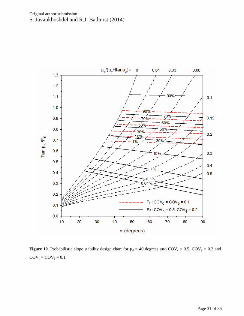
3.3 Simplified probabilistic slope stability design charts for c- soils

Figures 6 through 11 are simplified probabilistic stability design charts for the general case of

cohesive-frictional (c-) soils with μ = 20, 25, 30, 35, 40 and 45 degrees. The input parameters to

compute the conventional factor of safety F̅s are μc/(Htanμand as in the Steward et al. (2011)

chart. Hence, these charts provide an estimate of the conventional factor of safety for a slope using

mean estimates of the slope soil properties. Other values of μc/(Htanμcan be interpolated

between the long dash lines.



of 36

Superimposed on these charts are solid lines corresponding to probabilities of failure (Pf) assuming

maximum variability in the strength properties based on recommended values by Phoon and

Kulhawy (1999) (i.e. COVc = 0.5 and COV = 0.2). These curves are taken to 0.01% probability of

failure. Silva et al. (2008) reported that Pf = 0.01% (annual probability of failure) corresponds to an

earth dam designed to a factor of safety of 1.5 using above average level of engineering. The short

dash lines in the figures show example probability of failure curves using lower estimates of the

spread in c and (i.e. COVc = 0.1 and COV = 0.1). The spread of each set of these probability

curves is less because the COV for c and values is smaller. For these sets of curves, lines

corresponding to probability of failure of 1% and 0.01% are very close, therefore only lines

corresponding to 1% probability of failure are shown in the charts. The accuracy of Figures 6

through 11 was confirmed for the same ratios of μc/(Htanμbut using different values of μc,

and H in the SVSlope software.

For simple slope cases with the same slope angle and μc/H but other mean friction angles

between 20 and 45 degrees, the mean factor of safety can be linearly interpolated with mean friction

angle to sufficient practical accuracy as demonstrated by the plot in Figure 12. The logarithm of

the corresponding probability of failure also varies smoothly with mean friction angle showing that

log-linear interpolation between charts for Pf values is reasonable. The accuracy of the interpolation

curves was confirmed using the SVSlope software and a range of other values of μ COVc and

COV. The arrows in Figure 12 show that for the example case = 45 degrees, μ = 37 degrees

and μc/H = 0.05, the corresponding mean factor of safety is 1.42 and the probability of failure is

7%.

4 DISCUSSION

4.1 Influence of method of analysis

There are two options (Fixed and Floating Methods) in the SVSlope software to find the critical

slope and assign a probability of failure. The Fixed Method first locates the critical slip surface

based on a conventional deterministic slope stability analysis. Then, the factor of safety of this



of 36

single slip circle is recalculated using random values of the input soil parameters (i.e. Monte Carlo

simulation). The probability of failure is then computed as the fraction of outcomes with factor of

safety less than one. In the Floating Method, each trial slip surface is reanalyzed using random

variables of the soil input parameters. The probability of failure is then calculated as before using

all computed factors of safety from all simulations on all trial circles. This approach is

computationally more expensive but it is more general and in principle should give a more accurate

estimate of the true critical slip surface based on maximum probability of failure. Hence, the

Floating Method was used to generate the data to construct the design charts for c-soil cases in

this study.

It can be noted that Fixed and Floating methods were found to give the same mean factor of safety

(Equation 1) and probability of failure (Equation 10) for the case of cohesive soil slopes with no

spatial variability in soil parameters (i.e. the values in Figures 1 and 2).

For cohesive and c- soil cases when spatial variability is considered, results using the Fixed

Method were found to give lower probabilities of failure than the Floating Method. However, the

relative magnitude of the difference in Pf using both methods is less for the c-soil cases than the

cohesive soil cases. These observations are consistent with the remarks made by Cho (2010).

4.2 Influence of cross correlation between c and

The cross correlation () between strength parameters is considered to incorporate the dependence

between c and . A negative correlation between c and is reported in literature (Yucemen et al.

1973; Lumb 1970; Cherubini 2000) and implies that low values of friction angle are associated

with high values of cohesion and vice versa. The uncertainty in the calculated shear strength is

smaller when negative correlation between c and is considered rather than the combined

uncertainty in the two parameter values used to model the shear strength.

Figure 13 shows probability of failure versus mean factor of safety for the example slope with

μc/(Htanμ= 0.2 and COVc = 0.5 and COV = 0.2 and μ = 30 and different correlation

coefficients -1< < 0 (= 0 means that c and are uncorrelated parameters and = -1 means that c



of 36

and are highly correlated parameters). In Figure 13, the curve with = 0 is the same example

curve shown in Figure 4 which has probability of failure of 8% for the corresponding mean factor

of safety equal to 1.5. It can be seen in Figure 13 that for F̅s ≥ 1.08 the probability of failure Pf

decreases as the correlation coefficient becomes more negative. The implication is that the

probabilities of failure from Figures 6 to 11 are conservative for design.

4.3 Influence of spatial variability of c and

Spatial variability of soil strength parameters can be considered in SVSlope software using the

Distance Option (sampling distance). This option uses the Local Average Subdivision method

described by Fenton and Vanmarcke (1990) to model soil random fields in probabilistic slope

stability analysis. Sampling distance in the SVSlope software is equal to the scale of fluctuation.

The inset drawing in Figure 14 shows a constant distance (equal to scale of fluctuation) (L)

located along the arc length (L) of the circular slip. If distance L is equal to or greater than the arc

length then the same soil properties taken from random sampling are assigned to all slices during

each circular slip analysis. This is the default case used to generate the previous design charts. If the

distance (L) is less, new random soil values using the same soil property statistics for the control

case are assigned to each L segment. These random values are assigned to all slices whose base

mid-point falls within the same L segment (solid black circles). The correction method used in

SVSlope to treat a truncated L segment located at the end of the arc length has been taken from

Vanmarcke (1983). The method is described in the software manual and for brevity is not repeated

here.

The scale of fluctuation is taken as a twice the spatial correlation length θ (El-Ramly et al. 2003).

A large spatial correlation length value implies that the soil property is highly correlated over that

distance, resulting in a smooth variation within the soil profile. Conversely, a small value indicates

that the fluctuations of the soil property are large (El-Ramly 2001). Soil properties are typically

more variable in the vertical direction than the horizontal direction. El-Ramly (2001) and Phoon

and Kulhawy (1999) suggested values of autocorrelation length between 10 to 40 m and 1 to 3 m

in the horizontal and vertical directions, respectively. Figure 14 shows the influence of spatial

variability of soil strength parameters on probability of failure for an example slope. The upper



of 36

curve represents the idealized condition of no spatial variability in soil shear strength and is general.

The dashed curves are for the case with = 27 degrees, H = 10 m, D = 2 and = 17 kN/m3 and

different scale of fluctuation. The figure shows that as scale of fluctuation decreases (and spatial

variability of shear strength increases) the probability of failure decreases and all dashed curves are

sensibly less than the control case for F̅s > 1. Hence, for this case, Figure 2 can be considered to

give upper-bound estimates of probability of failure and is thus conservatively safe for design.

However, the potential influence of spatial variability on probability of failure will decrease as the

height of the slope decreases because autocorrelation lengths are independent of slope height and

geometry.

Cho (2007) reported two examples of probabilistic circular slip analysis using layered c- soils with

high factors of safety (F̅s > 1.5). These examples also gave decreasing probabilities of failure with

decreasing scale of fluctuation consistent with the trends in Figure 14 for the same range of factor

of safety.

Figure 15 shows the influence of normalized scale of fluctuation on probability of failure for

simple slope geometry and c- soil properties identified in the caption. It can be seen that for F̅s >

1, the probability of failure decreases with decreasing scale of fluctuation. The upper bound curve

(Θ = ∞) is the case when L ≥ L (spatial variability is not considered). The lower limit on Pf occurs

when each slice is resampled. In the limit of a very small slice width (x) the curves converge to

the deterministic value which is of no practical value. Furthermore, only those curves that

correspond to a scale of fluctuation at least twice the autocorrelation length of the soil properties are

of practical value as noted earlier.

4.4 Random finite element modeling

An alternative approach to investigation of the influence of spatial variation on probability of

failure of slopes is the use of the random finite element method (RFEM). Important references on

this approach are given in the introduction and in the textbook by Fenton and Griffiths (2008).

The method involves creation of a finite element mesh with each element assigned a random

property value. The distribution of property values may be random or spatially distributed. The soil



of 36

is assumed to behave as a linear-elastic plastic material and each finite element mesh with an

assignment of soil properties is taken as one realization. The finite element program redistributes

soil strength to satisfy the failure criterion and global equilibrium under gravity loading for each

realization. If the number of iterations to meet convergence criteria is greater than a prescribed

number, then the realization is assumed to represent failure. As in the probabilistic slope stability

method used in this paper, the number of realizations that fail divided by the total number of

simulations is the probability of failure.

At the time of the current study, RFEM slope stability methods are research tools and have yet to be

adopted by geotechnical engineers in practice and implemented in commercial slope stability

programs. However, the advantage of the RFEM method is that geometry of the critical failure

mechanism is not constrained, as is the case for conventional circular slip slope stability methods.

Each simulation will seek out the weakest path. This means that estimates of probability of failure

for the same nominal slope may be different between the RFEM slope stability approach and the

probabilistic slope stability approach adopted in the current study.

Griffiths and Fenton (2004, 2009, 2010) have shown that conventional probabilistic slope stability

analyses of the type used in the current study for cohesive soils may give non-conservative design

outcomes in some cases if spatial variability in the soil properties is not considered. Griffiths and

Fenton (2004) carried out random finite element method modelling of cohesive soil slopes for the

case when spatial variability in the soil properties is considered. They showed that when spatial

variability was included in the distribution of su for cases with deterministic F̅s > 1.37 and COVsu =

0.5, the probability of failure was less when spatial variability was included. The same is true in

Figure 14 for F̅s > 1 which was developed using the same slope geometry and soil properties as

Griffiths and Fenton (2004). The difference in the breakpoint value of deterministic F̅s = 1.37 in

their work and F̅s = 1 (Figure 14) is related to the difference in the way the critical mechanisms are

identified using these two methods and how spatial variability of soil properties is assigned to these

two very different approaches to probabilistic slope stability analysis. In many cases, the practical

minimum (mean) factor of safety for design of slopes is 1.5. Hence, the differences noted above can

be argued to be more of academic interest than practical concern.



of 36

5 CONCLUSIONS

The slope stability design charts developed in the current study apply to slopes with simple

geometry and random values of soil shear strength parameters su, c, and

The utility of the first chart (Figure 2) is that it allows the well-known Taylor (1937) chart (Figure

1) for cohesive soil slopes to be extended to include an estimate of the probability of failure for

each conventional mean factor of safety estimate. The chart in Figure 2 can be used for soils

having a range of coefficient of variation in su and matching the range reported in the literature.

Alternatively, the probability of failure can be calculated directly using the closed-form expression

(Equation 10) and values for the uncorrelated mean and coefficient of variation for the lognormal

distributions for su and .

The second series of charts (Figures 6 through 11) allow the conventional factor of safety to be

estimated for simple slopes with cohesive-frictional (c-) soil strength and simultaneously estimate

the corresponding probability of failure. These charts are presented for the case of maximum typical

estimates of coefficient of variation in c and . In this paper charts for μ = 20, 25, 30, 35, 40 and 45

degrees and μc ≥ 0 are presented. For other friction angle values within this range, the factor of

safety can be interpolated between charts.

Effects of cross correlation between strength parameters and spatial variability of strength

parameters on probability of failure are also considered in this paper. For F̅s > 1.08 and a negative

cross correlation between strength parameters c and (the usual case) probabilities of failure were

less than values for the idealized case of uncorrelated strength parameters. There is evidence in the

related literature that spatial variability in soil strength properties can also influence the probability

of failure for a soil slope. The probabilistic slope stability analyses of the type carried out in this

study showed that considering soil spatial variability will decrease the probability of failure of a

slope with F̅s > 1 when compared to the nominal identical simple slope case with point (random)

variability in soil shear strength values. Hence, the probabilities of failure using the design charts in



of 36

this paper may be considered to be conservative estimates (i.e. safe) for the analysis and design of

simple slopes.

It should be noted that estimating the variability of any soil property is difficult in practice and this

challenge is compounded when estimates of spatial variability are attempted for real world cases.

Consequently, the charts presented in this paper are useful for preliminary upper-bound estimates of

the conventional factor of safety and probability of failure of simple slopes with idealized soil

conditions and simple failure geometries (i.e. circular). In real world cases failure surfaces are often

irregular and therefore difficult to prescribe, and strongly coupled to spatial heterogeneity beyond

the scale of fluctuations in soil properties (e.g. layered soils). For cases involving layered soils and

more complicated surface geometry, probabilistic slope stability analyses can be carried out using

available commercial software packages or spreadsheet-based methods (e.g. Low et al. 1998, 2007;

Low 2003; Wang et al. 2010). Probabilistic slope analyses with layered soils introduce additional

challenges with respect to the number of searches to find the most critical mechanism. Strategies to

reduce computational effort for these cases can be found in the papers by Ching et al. (2009, 2010)

and Wang et al. (2010).

An important contribution of this paper is that it provides a link between probabilistic slope stability

analyses and the classical factor of safety approach which up until now has been difficult to

understand by many geotechnical engineers. By using simple cases this link is not obscured by

more complicated real world cases, complex mathematics and unfamiliar terminology. The

conservative outcomes using the idealized probabilistic approaches in this paper with respect to

classical factor of safety expectations are explained. The paper alerts the reader to the influence of

real world random and spatial variability of soil properties and large-scale heterogeneity due to

layering on computed probability of failure of slopes.

Finally, the charts presented in this paper are also useful for geotechnical engineers to check

computer-based probabilistic slope stability analysis outcomes against baseline cases.



of 36

ACKNOWLEDGMENTS

Financial support for this research was provided by the Natural Sciences and Engineering Research

Council of Canada (NSERC).

REFERENCES

Ang, A.H. and Tang, W.H. 1984. Probability concepts in engineering planning and design. Vol. 2.

Wiley, New York.

Baker, R. 2003. A second look at Taylor’s stability chart. J. Geotech. Geoenviron. Eng., 129(12):

11021108.

Cherubini, C. 2000. Reliability evaluation of shallow foundation bearing capacity on c, soils.

Canadian Geotechnical Journal

Ching, J.Y., Phoon K. K. and Hu, Y. G. 2009. Efficient Evaluation of Reliability for Slopes with

Circular Slip Surfaces using Importance Sampling. Journal of Geotechnical and

Geoenvironmental Engineering, ASCE, 135(6): 768777.

Ching, J.Y., Phoon, K.K. and Hu, Y.G.2010. Observations on Limit Equilibrium Based Slope

Reliability Problems with Inclined Weak Seams. Journal of Engineering Mechanics, ASCE,

136(10): 12201233.

Cho, S.E. 2007. Effect of spatial variability of soil properties on slope stability. Eng. Geol.

(Amsterdam), 92(3-4): 97109.

Cho, S.E. 2010. Probabilistic assessment of slope stability that considers the spatial variability of

soil properties. J. Geotech. Geoenviron. Eng., 136(7): 975–984.

Chowdhury, R.N. and Xu, D.W. 1993. Rational polynomial technique in slope reliability analysis,

J. Geotech. Eng. ASCE, 119(12): 19101928.

Chowdhury, R.N. and Xu, D.W. 1995. Geotechnical system reliability of slopes. Reliability

Engineering and System Safety, 47(3): 141151.

Christian, J.T., Ladd, C.C. and Baecher, G. B. 1994. Reliability applied to slope stability analysis, J.

Geotech. Eng. ASCE, 120(12): 21802207.

El-Ramly, H. 2001. Probabilistic analyses of landslide hazards and risks: Bridging theory and

practice. Ph.D. thesis, University of Alberta, Edmonton, Alta.



of 36

El-Ramly, H., Morgenstern, N.R. and Cruden, D.M. 2002. Probabilistic slope stability analysis for

practice. Canadian Geotechnical Journal, 39: 665–683.

El-Ramly, H., Morgenstern, N.R. and Cruden, D.M. 2003. Probabilistic stability analysis of a

tailings dyke on presheared clay shale. Canadian Geotechnical Journal, 40(1): 192208.

Fenton, G.A. and Griffiths, D.V. 2008. Risk Assessment in Geotechnical Engineering. John Wiley

& Sons, New York.

Fenton, G.A. and Vanmarcke, E.H. 1990. Simulation of random fields via local average

subdivision. Journal of Engineering Mechanics, 116(8): 17331749.

Fredlund, M.D. and Thode, R. 2011. SVSlope Theory Manual. SoilVision Systems Inc. Saskatoon,

Saskatchewan, Canada.

Geo-Slope Ltd. 2012. Slope/W for slope stability analysis: user’s guide. Calgary, Geo-Slope Ltd.

Griffiths, D.V. and Fenton, G.A. 2004. Probabilistic slope stability analysis by finite elements. J.

Geotech. Geoenviron. Eng., 130(5): 507518.

Griffiths, D.V., Huang, J. and Fenton G.A. 2009. Influence of spatial variability on slope reliability

using 2-D random fields. J. Geotech. Geoenviron. Eng., 135(10): 13671378.

Griffiths, D.V., Huang, J.S., Fenton, G.A., Fratta, D., Puppala, A.J. and Munhunthan, B. 2010.

Comparison of slope reliability methods of analysis. In Proceedings of GeoFlorida 2010:

advances in analysis, modeling and design, West Palm Beach, Florida, USA, 20-24 February

2010. pp. 19521961. American Society of Civil Engineers (ASCE).

Hong, H. and Roh, G. 2008. Reliability Evaluation of Earth Slopes. J. Geotech. Geoenviron.

Eng., 134(12): 1700–1705.

Huang, J., Griffiths, D.V. and Fenton, G.A. 2010. System reliability of slopes by RFEM. Soils and

Foundations, 50(3): 343353.

Li, K.S. and Lumb, P. 1987. Probabilistic design of slopes. Canadian Geotechnical Journal, 24:

520–535.

Low, B., Gilbert, R. and Wright, S. 1998. Slope reliability analysis using generalized method of

slices. J. Geotech. Geoenviron. Eng., 124(4): 350–362.

Low, B.K. 2003. Practical probabilistic slope stability analysis. Proceedings, Soil and Rock

America 2003, 12th Panamerican Conference on Soil Mechanics and Geotechnical Engineering

and 39th U.S. Rock Mechanics Symposium, M.I.T., Cambridge, Massachusetts, June 22-26,

2003, Verlag Glückauf GmbH Essen, Vol. 2, pp. 27772784.



of 36

Low, B.K., Lacasse, S. and Nadim, F. 2007. Slope reliability analysis accounting for spatial

variation. Georisk: Assessment and Management of Risk for Engineered Systems and

Geohazards, 1:4, 177189

Lumb, P. 1970. Safety factors and the probability distribution of soil strength. Canadian

Geotechnical Journal, 7: 225242.

Michalowski, R.L. 2002. Stability charts for uniform slopes. J. Geotech. Geoenviron. Eng., 128(4):

351355.

Phoon, K.K. and Kulhawy, F.H. 1999. Characterization of geotechnical variability. Can. Geotech.

J., 36(4): 612624.

Silva, F., Lambe, T.W. and Marr, W.A. 2008. Probability and risk of slope failure. Journal of

Geotechnical and Geoenvironmental Engineering, 134(12): 16911699.

Steward, T., Sivakugan, N., Shukla, S.K. and Das, B.M. 2011. Taylor’s slope stability charts

revisited. J. Geotech. Eng., 11(4): 348352.

Taylor, D.W. 1937. Stability of earth slopes. J. Boston Soc. Civ. Eng., 24(3): 197246.

Vanmarcke, E.H. 1977b. Reliability of earth slopes. Journal of the Geotechnical Engineering

Division, ASCE, 103: 1247–1265.

Vanmarcke, E.H. 1983. Random fields: analysis and synthesis. MIT Press, Cambridge, Mass.

Wang, Y., Cao, Z. and Au, S.K., 2010. Practical reliability analysis of slope stability by advanced

Monte Carlo simulations in a spreadsheet. Canadian Geotechnical Journal, 48(1): 162172.

Yuceman, M.S., Tang, W.H. and Ang, A.H.S. 1973. A probabilistic study of safety and design of

earth slopes. Civil Engineering Studies, Structural Research Series 402, University of Illinois,

Urbana, Ill.



of 36

Figure 1. Taylor’s slope stability chart for cohesive soils (Taylor 1937)



of 36

Figure 2. Probability of failure (Pf) versus (deterministic) mean factor of safety (F̅s) for cohesive

soil slopes with lognormal distribution of undrained shear strength (su) and unit weight (). Note:

Shaded region is the practical range. Dashed lines are for cases with COV = 0



of 36

Figure 3. Slope stability design chart for cohesive-frictional soils (after Steward et al. 2011).



of 36

Figure 4. Probability of failure (Pf) versus (deterministic) mean factor of safety (F̅s) for value of

μc/(Htanμ= 0.2 with μ = 30 degrees and a range of COV for strength parameter values



of 36

Figure 5. Probability of failure (Pf) versus (deterministic) mean factor of safety (F̅s) for COVc = 0.5 and

COV = 0.2 and a range of μc/(Htanμ



of 36

Figure 6. Probabilistic slope stability design chart for μ= 20 degrees and COVc = 0.5, COV = 0.2 and

COVc = COV = 0.1



of 36


COVc = COV = 0.1



of 36

Figure 12. (Deterministic) mean factor of safety and probability of failure from Figures 6 to 11 versus mean

friction angle μfor a range of μc/(H) for slopes with = 45 degrees and COVc = 0.5, COV = 0.2



of 36


COV = 0.2 and with μ = 30 degrees for negative values of cross correlation between c and



of 36

Figure 14. Example of influence of sampling distance on probability of failure (Pf) for slope for = 27

degrees, H = 10 m, D = 2, = 17 kN/m3, COVsu = 0.5 and COV = 0



of 36


COV = 0.2 with μ = 30 degrees for different normalized scale of fluctuation (= L/H)

Simplified probabilistic slope stability design charts for ... draft.pdf · Slope stability charts...

Documents

Transcript of Simplified probabilistic slope stability design charts for ... draft.pdf · Slope stability charts...