SIMPLIFIED EVALUATION METHOD OF

LIQUEFACTION-INDUCED RESIDUAL

DISPLACEMENT

Susumu YASUDA1, Nozomu YOSHIDA2, Kenji ADACHI3, Hiroyoshi KIKU4 and Keisuke ISHKAWA5

1 Member of JAEE, Professor, Div. of Architectural, Civil and Environmental Engineering,

Tokyo Denki University, Saitama, Japan, yasuda@g.dendai.ac.jp 2 Member of JAEE, Professor, Research Advancement and Management Organization

Kanto-Gakuin University, Yokohama, Japan, nyoshidan@kanto-gakuin.ac.jp 3 President, Jiban Soft Factory, Tokyo, Japan, adachi@jibansoft.com

4 Member of JAEE, President, Kanto Gakuin University, Kanagawa, Japan, kiku@kanto-gakuin.ac.jp

5 Member of JAEE, Assistant Professor, Div. of Architectural, Civil and Environmental Engineering, Tokyo Denki University, Saitama, Japan, ishikawa@g.dendai.ac.jp

ABSTRACT: A simplified method is proposed to obtain liquefaction-induced residual displacement. This method involves four procedures. First, the state of stress before an earthquake is calculated by an analysis considering the deposition and construction process of the ground. Next, the resistance factor against soil liquefaction, FL, is evaluated by a simplified liquefaction analysis. Then, post-liquefaction stress-strain relationships are evaluated from FL and liquefaction strength, RL. Finally, the difference between the initial stress and the stress evaluated by the post-liquefaction stress-strain relationships is applied as an external load (driving force) to a soil-structure model. A sequential laboratory test was conducted in order to obtain post-liquefaction stress-strain relationships, and these relationships were expressed as a function of RL and FL. Moreover, a stress-strain model for unliquefied layers, which is also important in evaluating liquefaction-induced flow, is proposed; it is an elastic-perfectly plastic model based on Mohr-coulomb and Dracker-Prager failure criteria. Two case histories showed that the simulated results agreed with actual earthquake damage.

Key Words: Liquefaction-induced flow, residual displacement, simplified procedure,

volume locking

- 1 -

1. INTRODUCTION It is well known that research on liquefaction was triggered by two earthquakes in 1964, i.e., the Niigata and Alaska earthquakes. Many buildings sank into the ground or tilted because the load-carrying capacity of the ground was diminished during the Niigata earthquake. After that, different type of damage was found. The Nihonkai-chubu earthquake in 1983 damaged gas pipelines on Maeyama hill in Noshiro City. Horizontal displacements on the order of several meters, discovered by comparing photographs taken before and after the earthquake, caused this damage1).This technique, comparing aerial photos before and after an earthquake, was applied to many past earthquakes 2) and large horizontal displacements were noted in many cases. Such ground displacement associated with soil liquefaction is called "liquefaction-induced flow" in this paper.

Effects to structures are quite different in these two phenomena. Structures settle in liquefied ground due to the ground’s loss of load-carrying capacity, but the large horizontal displacement of ground due to liquefaction imposes a load on structures above or near the ground, causing them to move.

As the liquefaction-induced flow occur in a widespread area, it is difficult to prevent it by local countermeasures, so structures built on ground susceptible to liquefaction must be strengthened to withstand the impact of liquefaction-induced flow3). In addition, as the design earthquake load was increased in many design specifications after the 1995 Kobe earthquake in Japan, it became more difficult to take remedial measures to prevent the onset of liquefaction. Therefore, structural strengthening has become popular to prevent damage due to soil liquefaction. The displacement of ground after the onset of liquefaction, which is called post-liquefaction displacement hereafter, must be predicted in order to design safe soil structures, such as river levees.

Seismic response analysis based on an effective stress (effective stress seismic response analysis, hereafter) has been considered one of the best ways to evaluate post-liquefaction displacement. However, the results of many effective stress seismic response analyses vary significantly depending on the computer program used (e.g. refs. 4 and 5), which may be due to the differing concepts of the programs used or due to the differing skills of the engineers applying the programs. Moreover, effective stress seismic response analysis is difficult to perform because it requires the evaluation of many parameters. As an alternative method, the authors proposed a simplified method named ALID (Analysis for Liquefaction-Induced Displacement) 6). This is a static analysis to evaluate residual displacements after an earthquake by using a post-liquefaction stress-strain curve based on the concept that only the load of gravity applies after an earthquake. In the previous report6), fundamental concepts and stress-strain models for the post-liquefaction behavior for the ALID method were proposed, and some notes in the practical analysis were added. This method has been used to evaluate the post-liquefaction displacement of many types of structures, including soil structures, and the authors have attempted to improve the accuracy of the method, as reported in this paper with case studies.

2. BRIEF REVIEW OF PAST RESEARCHES

In its early stage, soil liquefaction research did not focus on liquefaction-induced displacement because liquefaction was recognized to be a failure of the ground. For example, Seed et al., in discussing the mechanism of the failure of the Lower San Fernando dam7), attributed the deformation of the dam over time to a decrease of liquefaction strength caused by a decrease of effective stress, but they did not discuss displacement. Figure 1 is a graph by these authors of residual strength back-calculated from sites of liquefaction8), but residual displacement was not considered.

Figure 2 shows general features of post-liquefaction behavior9). Similar figures are shown in other research, such as in ref. 10). In these figures, shear stress decreases to the residual stress after peaking, as shown in ref. 7) and other past research. Figure 2 also shows that stress increases or recovers in dense sand, so the sand remains stable even after liquefaction. On the other hand, stress does not recover in loose sand, which results in failure due to liquefaction-induced flow. However, actual stress-strain behavior is not discussed in this research; the stress-strain curve shown in Figure 2 may have come from an image of

- 2 -

the stress-strain curve under monotonic loading. According to reference 9), which contains Figure 2, residual strength is more than 1 MPa for sand with a relative density of 38%, the loosest existing sand, and is about 30 kPa for sand with a relative density of 19%, looser sand that does not exist in the field.

This research differs from Japanese "liquefaction-induced flow" quite a bit. Over several meters displacement is frequently observed in nearly horizontal ground or ground at a surface gradient of 1/100 in Japan. In ground with liquefiable layers of several meters thick and a 1/100 surface gradient, for example, the initial stress at an overburden stress of 100 kPa is about 1 kPa, which is much smaller than the shear stress (about 1MPa) in ref. 9). There is, unfortunately, nearly no data on post-liquefaction residual strength, but it is obvious that these Japanese cases cannot be explained by the stress-strain curve in ref. 9).

The authors propose the two mechanisms shown in Figure 3 to explain post-liquefaction behavior11). The solid line graph, ABCD (or D' for dense sand) is the same as the bottom line graph in Figure 2. Here, if the initial stress before an earthquake (1 in Figure 3) is greater than the residual stress, unstable liquefaction-induced flow can occur, and it is difficult or impossible to predict the displacement. On the other hand, if the maximum shear stress during an earthquake (2 in Figure 3) is less than the peak strength, f, or if the residual strength after liquefaction is larger than the working stress, the ground remains stable, as shown by the dashed line OB, its behavior can be evaluated by displacement criteria, and its deformation can be predicted.

A laboratory test was carried out in our previous study6) based on these concepts. After loading the cyclic shear stress up to liquefaction or more, shear strain was monotonically increased to obtain post-liquefaction stress-strain relationships. Some examples of the stress-strain relationships thus obtained are shown in Figure 4. The ranges of shear strain with nearly zero stiffness, during which liquefaction-induced

Figure 1 Residual strength obtained by back analysis8)

Figure 2 Image of post-liquefaction behavior9)

Figure 3 Two mechanisms on post-liquefaction behavior

Figure 4 Example of post-liquefaction behavior (vertical axis is enlarged in

(b) from (a))

0

10

20

30

40

50

Equivalent clean sand, (N1)60

Res

idua

l str

engt

h (kPa

)

0 5 10 15 20

Non-flowDilativeor strainhardeningbehavior

Flow

Contractiveor strainsofteningbehavior

Flow withlimited deformation

Flow

Shear strain

She

ar s

tres

s

(b)

She

ar s

tres

s

Shear strain

1

2

f

A

B

C

O

Deformation criterion

Stability criterion

DE

E

Monotonic loadingDense sandPost-liquefaction bebavior

D'

StaticFL=0.95 FL=0.89FL=1.0

FL=0.72FL=1.13

StaticFL=0.72

FL=0.89FL=1.0

FL=1.13 FL=0.95

She

ar s

tres

s (k

Pa)

She

ar s

tres

s (k

Pa)

1.0

0.5

0

200

150

100

50

06050403020100

403020100

Shear strain (%)

Shear strain (%)

(a)

(b)

Toyoura sand, Dr=50%

'0=98 kPa

- 3 -

flow occurs, increase as FL decreases, as shown in Figure 4 (a). However, Figure 4 (b), in which the vertical axis of Figure 4 (a) is enlarged, shows some stiffness in this flow region, although it is very small. Therefore, shear stress is less than 1 kPa even when shear strain reaches several tens of percent. Japanese cases of horizontal displacement of several meters can be explained by these stress-strain relationships.

Another important piece of information needed to predict the displacement caused by liquefaction-induced flow is the time the flow occurred. The displacement of the Lower San Fernando dam occurred after an earthquake7). The 1964 Niigata earthquake caused a slab of the Showa Bridge to collapse and cracks in the river levee near the bridge. The bridge collapsed about 70 seconds after the beginning of the earthquake and cracks in the river levee appeared after that 12 ). These observations indicate that liquefaction-induced flow occurs after a main shock or when ground shaking is nearly terminated.

If liquefaction-induced flow occurred after the ground shaking, it would be due only to the force of gravity. Therefore, if we focus on the residual state, we can analyze liquefaction-induced flow using the post-liquefaction stress-strain model shown in Figure 4. This is the basic concept of ALID.

3. POST-LIQUEFACTION SHEAR DEFORMATION CHARACTERISTICS

3.1 Brief review of laboratory test result in the previous study In our previous study6), post-liquefaction stress-strain behavior, which is necessary for ALID analysis, was obtained by cyclic loading tests on Toyoura sand that did not include fines and on silty sand which included fines of 20–30%. Figure 5 shows the loading program for these tests schematically. The test specimen was consolidated under isotropic stress identical to the in-situ overburden stress. Then, cyclic shear stress was applied under undrained condition identical to the cyclic shear stress applied in conventional liquefaction tests at pre-determined cycles. Finally, a monotonic load was applied to the undrained specimen. The stress-strain behavior at this stage was considered post-liquefaction behavior. The stress-strain curve obtained from a specimen just beginning to liquefy differed from the stress-strain curve obtained from a specimen after liquefaction because the degree of liquefaction varied. The resistance factor against soil liquefaction, FL, (liquefaction resistance factor, hereafter) expresses the severity of liquefaction. Loading is controlled by shear stress amplitude while keeping the number of loadings at 20; FL value is calculated as the ratio of shear stress amplitude to the shear stress amplitude at the moment of liquefaction.

Figure 4 shows the stress-strain curves with different FL values from tests carried out with FL, relative density, and initial

Figure 5 Method of loading on shear stress

Figure 6 Test result for Toyoura sand under FL=1.0 with different relative density (vertical axis is

She

ar s

tres

s Consolidation

Monotonic

loading

Time

Exc

ess

PW

P

Liquefaction

Time

Cyclic loading

(a)

Toyoura Sand200

150

100

50

06050403020100

'0=49 kPa

Dr=65.9%FL=1.0u/'0=1.0

Dr=53.9%

Dr=32.6%Dr=-5.2%

(b)1.0

0.5

0403020100

Dr=65.9%

Dr=53.9%

Dr=32.6%

Dr=-5.2%

- 4 -

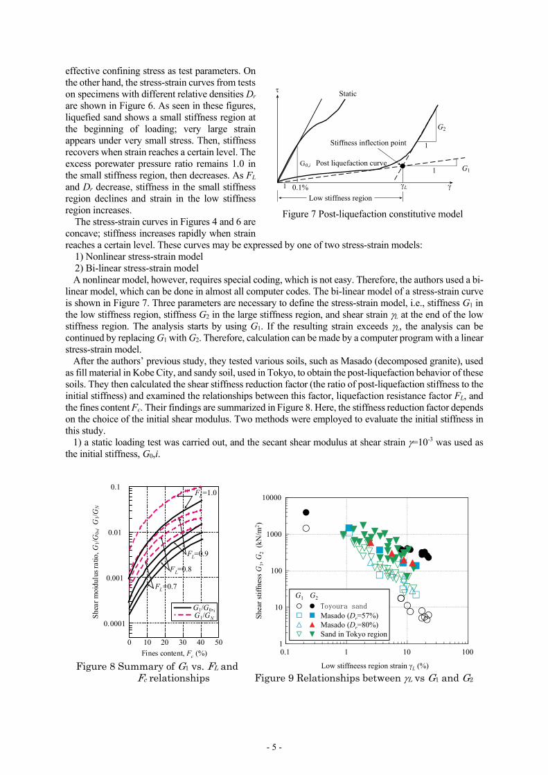
effective confining stress as test parameters. On the other hand, the stress-strain curves from tests on specimens with different relative densities Dr are shown in Figure 6. As seen in these figures, liquefied sand shows a small stiffness region at the beginning of loading; very large strain appears under very small stress. Then, stiffness recovers when strain reaches a certain level. The excess porewater pressure ratio remains 1.0 in the small stiffness region, then decreases. As FL and Dr decrease, stiffness in the small stiffness region declines and strain in the low stiffness region increases.

The stress-strain curves in Figures 4 and 6 are concave; stiffness increases rapidly when strain reaches a certain level. These curves may be expressed by one of two stress-strain models:

1) Nonlinear stress-strain model 2) Bi-linear stress-strain model A nonlinear model, however, requires special coding, which is not easy. Therefore, the authors used a bi-

linear model, which can be done in almost all computer codes. The bi-linear model of a stress-strain curve is shown in Figure 7. Three parameters are necessary to define the stress-strain model, i.e., stiffness G1 in the low stiffness region, stiffness G2 in the large stiffness region, and shear strain L at the end of the low stiffness region. The analysis starts by using G1. If the resulting strain exceeds L, the analysis can be continued by replacing G1 with G2. Therefore, calculation can be made by a computer program with a linear stress-strain model.

After the authors’ previous study, they tested various soils, such as Masado (decomposed granite), used as fill material in Kobe City, and sandy soil, used in Tokyo, to obtain the post-liquefaction behavior of these soils. They then calculated the shear stiffness reduction factor (the ratio of post-liquefaction stiffness to the initial stiffness) and examined the relationships between this factor, liquefaction resistance factor FL, and the fines content Fc. Their findings are summarized in Figure 8. Here, the stiffness reduction factor depends on the choice of the initial shear modulus. Two methods were employed to evaluate the initial stiffness in this study.

1) a static loading test was carried out, and the secant shear modulus at shear strain =10-3 was used as the initial stiffness, G0,i.

Figure 8 Summary of G1 vs. FL and

Fc relationships

Figure 9 Relationships between L vs G1 and G2

0 10 20 30 40 50

Fines content, Fc (%)

0.0001

0.001

0.01

0.1

She

ar m

oidu

lus

ratio

, G1/

G0,

i G

1/G

N

G1/G0,iG1/GN

FL=0.9

FL=0.8

FL=0.7

FL=1.0

1

10

100

1000

10000

10 100

Low stiffneess region strain L (%)

0.1 1

G1 G2

Toyoura sandMasado (Dr=57%)Masado (Dr=80%)Sand in Tokyo region

Figure 7 Post-liquefaction constitutive model

Post liquefaction curve

Static

G2

G11

1

G0,i

L 0.1%1

Low stiffness region

Stiffness inflection point

- 5 -

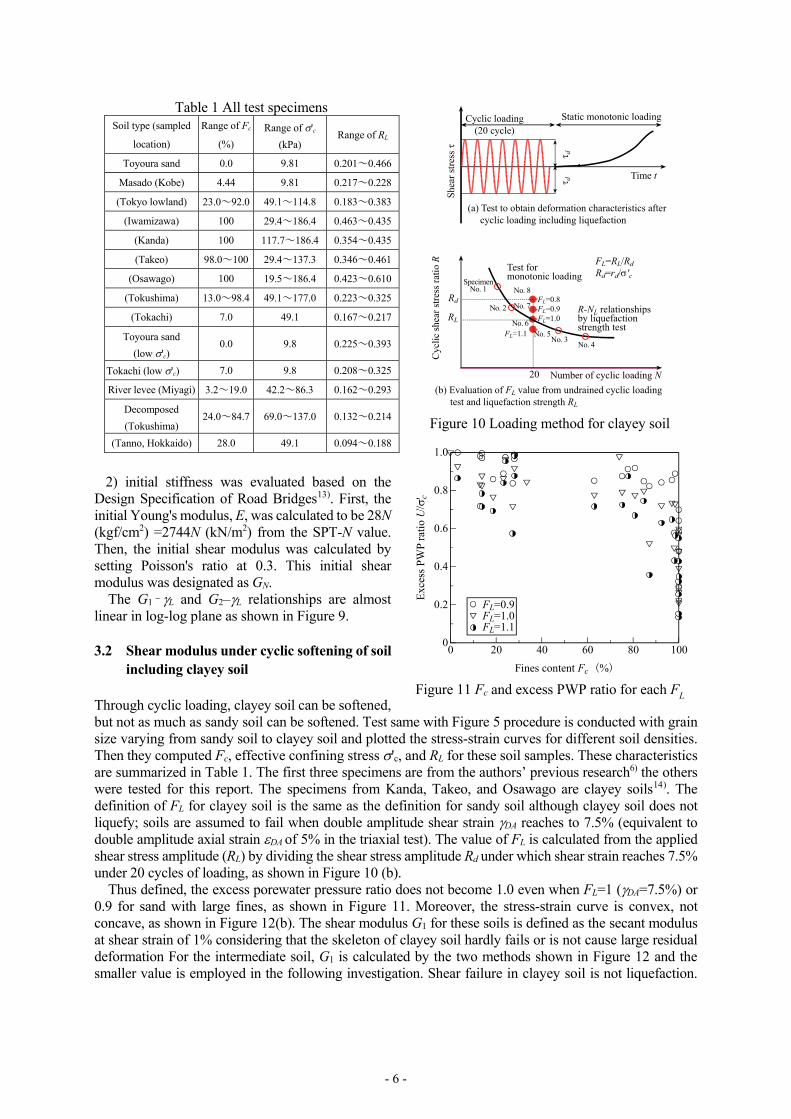
2) initial stiffness was evaluated based on the Design Specification of Road Bridges13). First, the initial Young's modulus, E, was calculated to be 28N (kgf/cm2) =2744N (kN/m2) from the SPT-N value. Then, the initial shear modulus was calculated by setting Poisson's ratio at 0.3. This initial shear modulus was designated as GN.

The G1–L and G2–L relationships are almost linear in log-log plane as shown in Figure 9.

3.2 Shear modulus under cyclic softening of soil

including clayey soil Through cyclic loading, clayey soil can be softened, but not as much as sandy soil can be softened. Test same with Figure 5 procedure is conducted with grain size varying from sandy soil to clayey soil and plotted the stress-strain curves for different soil densities. Then they computed Fc, effective confining stress 'c, and RL for these soil samples. These characteristics are summarized in Table 1. The first three specimens are from the authors’ previous research6) the others were tested for this report. The specimens from Kanda, Takeo, and Osawago are clayey soils14). The definition of FL for clayey soil is the same as the definition for sandy soil although clayey soil does not liquefy; soils are assumed to fail when double amplitude shear strain DA reaches to 7.5% (equivalent to double amplitude axial strain DA of 5% in the triaxial test). The value of FL is calculated from the applied shear stress amplitude (RL) by dividing the shear stress amplitude Rd under which shear strain reaches 7.5% under 20 cycles of loading, as shown in Figure 10 (b).

Thus defined, the excess porewater pressure ratio does not become 1.0 even when FL=1 (DA=7.5%) or 0.9 for sand with large fines, as shown in Figure 11. Moreover, the stress-strain curve is convex, not concave, as shown in Figure 12(b). The shear modulus G1 for these soils is defined as the secant modulus at shear strain of 1% considering that the skeleton of clayey soil hardly fails or is not cause large residual deformation For the intermediate soil, G1 is calculated by the two methods shown in Figure 12 and the smaller value is employed in the following investigation. Shear failure in clayey soil is not liquefaction.

Table 1 All test specimens Soil type (sampled

location)

Range of Fc

(%)

Range of 'c

(kPa) Range of RL

Toyoura sand 0.0 9.81 0.201～0.466

Masado (Kobe) 4.44 9.81 0.217～0.228

(Tokyo lowland) 23.0～92.0 49.1～114.8 0.183～0.383

(Iwamizawa) 100 29.4～186.4 0.463～0.435

(Kanda) 100 117.7～186.4 0.354～0.435

(Takeo) 98.0～100 29.4～137.3 0.346～0.461

(Osawago) 100 19.5～186.4 0.423～0.610

(Tokushima) 13.0～98.4 49.1～177.0 0.223～0.325

(Tokachi) 7.0 49.1 0.167～0.217

Toyoura sand

(low 'c) 0.0 9.8 0.225～0.393

Tokachi (low 'c) 7.0 9.8 0.208～0.325

River levee (Miyagi) 3.2～19.0 42.2～86.3 0.162～0.293

Decomposed

(Tokushima) 24.0～84.7 69.0～137.0 0.132～0.214

(Tanno, Hokkaido) 28.0 49.1 0.094～0.188

Figure 10 Loading method for clayey soil

Figure 11 Fc and excess PWP ratio for each FL

(a) Test to obtain deformation characteristics after cyclic loading including liquefaction

(b) Evaluation of FL value from undrained cyclic loading test and liquefaction strength RL

Test formonotonic loading

FL=RL/Rd

Rd=rd/'c

Rd

RL

No. 2

SpecimenNo. 1

No. 3No. 4

No. 5No. 6

No. 7

No. 8FL=0.8FL=0.9FL=1.0

FL=1.1

20

R-NL relationshipsby liquefactionstrength test

Number of cyclic loading N

Cyclic loading(20 cycle)

Static monotonic loading

Time t

Fines content Fc (%)

FL=0.9FL=1.0FL=1.1

0

0.2

0.4

0.6

0.8

1.0

0 20 40 60 80 100

- 6 -

Strictly speaking, it is called "shear failure under undrained cyclic loading", but we call it liquefaction for simplicity because ALID was originally developed for sandy soil.

When clayey soils are included in a soil specimen, the calculations summarized in Figure 8 are complicated. The behavior of clayey soil cannot be well explained only by its fines content Fc. Originally, Fc is employed to consider the empirical fact that the degree of degradation or softening depends on grain size. RL is chosen as an alternate to Fc because RL has the same characteristics as Fc for sandy soil. Moreover, the ratio of G1 to the initial shear modulus is used in the ordinate of Figure 8, and the initial shear modulus is evaluated from the SPT-N value or from a laboratory test. In clayey soil, however, the evaluation of the initial shear modulus is sometimes difficult because the SPT-N value is small. In addition, G1 is affected by the initial confining stress 'c, which should be considered in the empirical equation. The relationship between G1 and 'c is shown in Figure 13 in a double logarithmic axis; it is nearly linear and the slope of the line is nearly 1. Iwasaki et al. showed that the effect of 'c on cyclic shear modulus G increases and that G1 is proportional to the first power of 'c at a shear strain of =10-2 based on their test results or on the cyclic shear modulus obtained from a wide range of strain15). The G1 values used in this research deal with the same order of strain. In other words, tests in this research and those by Iwasaki et al., are in harmony to each other. Taking these factors into account, the ratio of G1 to the initial confining stress 'c. is employed as the ordinate of the graph in Figure 14, which shows the relationships between the liquefaction strength ratio RL and the shear modulus ratio G1/'c with FL as a parameter. As seen in the figure, the correlation is good for each value of FL. The relationship is formulated as

exp( ( ))1 / ' Lb R c

cG ae σ for 0.8<FL<1.1 (1)

where 23.6 0.98La F 3 29.32 10.8 13.27 0.806L L Lb F F F , 3 21.40 3.87 4.14 1.95L L Lc F F F .

Figure 12 Two types of softening stress-strain curve and definition of parameters such as G1.

Figure 13 Effect of confining Figure 14 Relationships between liquefaction

strength and shear modulus ratio at

Shear strain

(a) Type A

L

G1

G2(b) Type B

Shear strain 1%

G1

1 5 10 50 100 5001

5

10

50

100

500

Effective confining stress, 'c (kPa)

G1=0.32'c0.86

Tokachi sand, FL=0.9Dr=70% (Fc=7%)Dr=85% (Fc=7%)

Liquefaction strength RL (DA=7.5%, NL=20)

0 0.1 0.2 0.3 0.4 0.5 0.6 0.7 0.810-3

10-2

10-1

100

101

102

Type A BFL=0.8FL=0.9FL=1.0FL=1.1

FL=1.0FL=1.1

FL=0.8FL=0.9

- 7 -

As can be seen in Figure 14, the shear modulus of clayey soil with RL greater than 0.35 is several tens of times larger than that of loose sand even if FL=0.9, which indicates that large residual deformation hardly occurs in clayey soil. In addition, the stress-strain curve conforms to Type B when RL>0.35.

3.3 Estimation of stiffness for FL<0.8

The previous test shown in Figure 10(a) can be done only for FL greater than about 0.8 because of limitations of the test equipment and test method. When conducting the test with FL<1, cyclic loading is to be continued after the onset of liquefaction. Shear strain increases rapidly in this case. On the other hand, cyclic loading is limited by the ability of a cylinder stroke to apply large cyclic loading. For these reasons, testing with FL<0.8 is difficult.

Analysis with smaller FL value is, however, necessary for design under so-called level 2-ground motion (very severe ground shaking). Hence, it is necessary to extend Eq. (1) to FL smaller than 0.8. The cyclic torsional shear test is not applicable under smaller FL, but back analysis could be used. Toyoda et al16), for example, evaluated stiffness under low FL value from the back analysis of damage to river levees. In this research, 10 river levees that were damaged during the 1995 Kobe earthquake and the 1994 Hokkaido-nansei-oki earthquake, etc. were investigated. The post-liquefaction shear moduli calculated for small FL values are shown in Figure 15. This figure shows the relationship between G1/'c and FL with RL as a parameter, whereas Figure 14 shows the relationship between G1/'c and RL as FL a parameter, which agrees with Eq. (1) for FL0.8.

4. DEFORMATION ANALYSIS BY MEANS OF FINITE ELEMENT METHOD

4.1 Procedure of analysis

Soil liquefaction causes deformation when the soil skeleton is destroyed by earthquake motion or when excess porewater pressure dissipates. Deformation of soil also occurs during ground shaking, but it is supposed to be much smaller than the displacement caused by liquefaction-induced flow and is neglected in this research.

The effective stress decreases as the soil skeleton collapses due to the cyclic shear generated by an earthquake. This results in a decrease of stiffness and strength and an increase of excess porewater pressure. Deformation during this process can be attributed to the inability of the soil skeleton to carry the load before the earthquake. Therefore, it is important to evaluate both the stress state before an earthquake and the stiffness after liquefaction. Details of this analysis are explained in the next section. The stress state before an earthquake is evaluated through initial stress analysis. The FL value is first evaluated by liquefaction analysis, then

Figure 15 FL-RL relationships under FL<0.8

(Toyoda et al.16))

Figure 16 Schematic figure to obtain

liquefaction-induced flow

0.0 0.2 0.4 0.6 0.8 1.0 1.2

FL

Shear strain

G2

G1LS

hear

str

ess

Embankment

Pick uppoint

Foundation ground

Liquefied layer

Non-liquefied layer

0.0001

0.001

0.01

0.1

1

10

100

G1/'

c

RL=0.20

RL=0.25

RL=0.30

RL=0.35

RL=0.40

RL=0.45RL=0.50

RL=0.15

No. 1, 2, 3, 4, 5, 7, 8No. 6, 9, 10No. 6, 9, 10 (Based on RL)

1

2

AB

O

C

0

1

1

L

m

- curve before eq.

- curve during flow

G1

G2

- 8 -

analysis using the FL dependent stress-strain curve shown in previous section is performed to obtain the deformation.

This process is schematically shown in Figure 16. The state before the earthquake, which is obtained by initial stress analysis, is designated as A. If seismic response analysis based on an effective stress is conducted, the stress path is expressed by the dashed line A B. However, in this analysis, the stress-strain curve OCB is used, and it is obtained from the FL value evaluated from liquefaction analysis. The stress difference m between the stress-strain curves before and after liquefaction at strain 0 is applied as the external load following the path A C B.

Finally, simplified consolidation analysis is conducted to obtain the subsidence of ground due to excess porewater pressure dissipation.

For this analysis, the authors assumed 1) a plane stress state, 2) small strain, and 3) no change in the volumes of soil particles and porewater. In addition, the authors distinguished saturated soil layers from unsaturated layers and did not consider porewater pressure for the unsaturated soil. The analysis was conducted using the equation governing two-phase materials to distinguish the behavior of the soil skeleton from the behavior of the porewater.

4.2 Method of analysis at each procedure (1) Initial stress analysis

It is important to evaluate the stress state before an earthquake accurately because liquefaction-induced displacement is driven by the initial stress. Generally, the analyzed ground has been altered from the original natural deposit. Therefore, initial stress must be analyzed following the process of ground modification. Figure 17 shows an example of a river levee shown in Section 0. A switch-on-gravity analysis is conducted first to obtain the natural deposition state (Holocene sandy layer, As, and clayey layer, Ac), where the water table is located at the ground surface. Then surface ground is added. Next, construction of the river levee is simulated by several stage banking analyses (sometimes called layer construction analysis). Finally, the water table is returned to its state just before the earthquake.

In this case study, as the inclination of the levee slope is a little steep, considering the levee height (about 7 m), soil failure is suspected in the liquefiable foundation ground and in the embankment. Therefore, the liquefiable layer and the embankment material including surface soil are modeled as an elastic-plastic material, described later. Moreover, layer construction analysis is necessary for these soils. Seepage force during the change of water table in the steady state analysis is negligibly small, but as stiffness becomes very small in the liquefaction-induced flow analysis (flow analysis, hereafter, for simplicity), non-negligible deformation may occur under the small seepage force. This indicates that the relevant porewater pressure must be calculated by seepage analysis when the water table tilts.

(2) Liquefaction analysis

The value of FL is to be evaluated following the initial stress analysis in order to analyze the liquefaction induced flow. In other words, the onset of liquefaction is to be evaluated separately and independently. Since the FL value is defined as the ratio of liquefaction strength RL to the cyclic shear stress ratio L generated during an earthquake, these two values must be evaluated. Two methods can be used to estimate these values; one simple, the other detailed. When long or wide areas in dangerous locations, such as long

Figure 17 Procedure of initial stress analysis

S w itch -on g rav ity ana ly s iso f n a tu ra l d ep o sit

(H orizon ta l w ate r tab le)

A c

R iv er chan ne l

A s

A c

A s

A c

A s

A c

A s

P repara tio n o f su rface lay er L ay er co n s tru c tio n o fem b ank m en t

(sev eral s tep an a lysis)

C han ge o f w ate r tab le(w a te r leve l d iffe ren ce

be tw een b o th s ides )

- 9 -

river levees, are analyzed, the simple method is relevant. On the other hand, detailed analysis is encouraged when evaluating the subsidence of individual structures.

In the detailed analysis, the liquefaction strength RL is evaluated by a laboratory test on an undisturbed sample. This method was used to calculate RL in Figure 10 and G1 and G2 in Figure 12 simultaneously. Moreover, volumetric strain v, described in section 4.2 (4), which is necessary to evaluate ground subsidence after the dissipation of excess pore water pressure, can also be obtained at the same time. As described in section 3.3, however, laboratory tests are difficult to perform when FL is less than 0.8. Therefore, a back-analyzed value of FL, such as the values shown in Figure 15, is used in conjunction with laboratory test results.

Several methods have been proposed to evaluate RL from SPT-N value and fines content, and design specifications, such as Specifications for Highway Bridges13) and Recommendations for Design of Building Foundations17), have been used in practice in Japan. In this case, G1 is evaluated first from Figure 8 or Figure 14, and L is read off from Figure 9 by using G1. Finally, G2 is read off from Figure 9 at L. Volumetric strain v after the dissipation of excess pore water pressure can be evaluated from FL and relative density Dr, etc. using the empirical equations proposed by, for example, Ishihara and Yoshimine18) and Tsukamoto et al.19).

On the other hand, seismic response analysis is conducted to obtain L in the detailed method. The cyclic shear stress in each element is calculated by seismic response analysis, and this stress is divided by the initial effective confining stress to obtain L. Initial effective confining stress is constant in the horizontal direction in horizontally deposited ground, but it is not constant when structures and/or fill sit on the ground. The initial effective confining pressure in ground beneath a structure or fill is larger than the initial effective confining pressure in a horizontally layered deposit. The effective confining stress used in the initial stress analysis can be used for ground beneath a structure or fill.

Equations to evaluate L in design specifications, such as Specifications for Highway Bridges13) and Recommendations for Design of Building Foundations17), can be used to obtain L in the simplified method. It is important to consider that confining pressure is larger in soil under or near a structure or fill than it is in a horizontally layered deposit. Moreover, the maximum shear stress in soil under or near a structure or fill differs from the maximum shear stress in a horizontally layered deposit. Considering these facts, the simplified method entails a certain degree of error.

(3) Liquefaction-induce flow analysis

The procedure of flow analysis is schematically shown in Figure 16. Since plane strain condition is assumed in this research, and in the figure are read to maximum shear stress m={(x-y)2/4+2

xy}0.5 and maximum shear strain m={(x-y)2+}0.5, where and are normal stress and strain, respectively, and subscripts x and y denote horizontal and vertical directions, respectively. In the analysis, the stress-strain curve changes suddenly from one before an earthquake (dotted line) to one after liquefaction (solid bi-linear line). For example, the state point moves from A to C. The difference between the shear stress or unbalanced stress between points A and C, 21 mmm , is applied as a driving force, resulting in the movement of the state point from C to B. Since the undrained condition is assumed in this analysis, excess pore water pressure equivalent to the initial effective stress is generated, and the axial component of shear stress m1 disappears, as it does in practice. As m is composed of only an axial component and horizontal displacement is restricted in horizontally layered ground, all of m is transferred into pore water pressure; therefore, point C does not move or flow deformation does not occur.

As easily understood from the preceding explanation, driving force significantly affects the initial stress state; therefore, initial stress analysis is important. As the driving force is released in the path A C, this method is called the "stress relaxation method". In our previous study6), another method called the "switch-on-gravity method" was introduced. This method is based on the switch-on-gravity analysis starting from O or C. When initial stress is calculated through several processes, however, this method is sometimes less accurate than the stress relaxation method. Therefore, the switch-on-gravity method is not employed in this study.

- 10 -

Since an undrained condition is assumed in the liquefied and saturated soil element, the incremental equilibrium equation is expressed as

00

pi i

Tip

K K u F

pK

(2)

Here, brackets [ ] and braces { } denote matrix and vector, respectively, u denotes nodal displacement of the soil skeleton, p denotes pore water pressure, denotes incremental quantity, and subscript i denotes i-th step of incremental analysis. Stiffness matrix [K] is calculated by a reduced integration to avoid volume locking behavior, as explained in the next section.

T

c c EK B D B V (3)

where [B] denotes the strain-displacement matrix, subscript c indicates the value at the center of an element, and VE denotes the area of an element. Matrix [D] is a stress-strain matrix and is expressed under the plane strain condition as

4 23 3

2 43 3

0

[ ] 0

0 0

K G K G

D K G K G

G

(4)

where K and G denote bulk modulus and shear modulus, respectively. Shear modulus G takes the value G1 or G2 in Figure 7, depending on whether the shear strain is greater than or less than L, respectively. {Kp}=[B]T{m}VE is a porewater vector, where {m}={1 1 0}T is a matrix expression of the Kronecker's delta.

The right side of Eq. (2) is the external load in an incremental calculation and is expressed as

1 1

1ii p i

i

F F F K pN (5)

where {F} denotes the nodal force equivalent to stress and pore water pressure at the start of the analysis, and {Fi-1}=[B]T{i-1}VE denotes the nodal force equivalent to stress before the incremental calculation. Here, i-1 and pi-1 denote stress and pore water pressure in the element, respectively. The term in parentheses on the right side of Eq. (5) is a driving force, which is not applied at the end of the i-1-th incremental calculation, and is applied as a driving force after dividing by Ni in the i-th incremental analysis. When incremental analysis is carried in N steps, Ni=N–i+1. As the state point is located at C in Figure 16 at the beginning of the analysis, some stress is already working. The initial force vector is evaluated for a given strain 0 as

0 1 0{ } [ ] [ ]{ } T

cF B D V (6)

where [D1] is a matrix in which G1 is substituted for G in Eq. (4). The definition of 0 is clear in the simple case such as in Figure 16. However, when layer construction and excavation analyses are repeated, 0 cannot be obtained simply. In this case, {0} is obtained from the shear stress {1} at point A by dividing elastic modulus [D]. As both 0 and G1 are nearly zero, this term does not affect the result of analysis.

As there is no relaxing stress in the non-liquefied element in the first incremental analysis ({ } {0} iF ), but stress and pore water pressure change depending on the deformation of other elements, the right side of Eq. (2) yields,

1 1

T

i c i E p iF F B V K p (7)

Finally, since porewater pressure p0 in the unsaturated elements, the term p can be eliminated in Eq. (2).

(4) Post-liquefaction subsidence due to the dissipation of excess pore water pressure

- 11 -

Excess pore water pressure is generated in the preceding analysis. Volume compression occurs as this excess pore water pressure dissipates. This process is expressed in Eq. (2) as

1 0

1ii p

i

K u F F K pN

(8)

where p0 is pore water pressure before liquefaction. The stress-strain matrix included in [K] includes plastic volumetric change due to dilatancy, but linear analysis is carried out using an apparent equivalent modulus for simplicity, as shown below.

Volumetric strain caused by the dissipation of excess pore water pressure can be obtained from empirical equations, such as ref. 18) and 19). This volumetric change is assumed to occur only in the vertical direction. Then, the vertical stress y caused by the volumetric change yields

4

3y c c vp K G

(9)

where p is excess pore water pressure generated during the flow and is a known quantity. In addition, the apparent Poisson's ratio during one-dimensional compression is assumed to be 1/3. Then, the apparent bulk modulus c and shear modulus Gc used in Eq. (8) are obtained by coupling Poisson's ratio with Eq. (9), which yields

1

4cv

pG

,

2 1 8

3 1 2 3c c cK G G

(10)

This method shows that volumetric strain is affected by the interaction between neighboring elements and stiffness, and this interaction is expressed by Eq. (10). 4.3 Some notes on the analysis (1) Avoidance of volume rocking

Poisson's ratio sometimes approaches 0.5 in the total stress analysis of ground. Volume change hardly occurs in this case, which causes underestimation of deformation, called volume locking. For example, volume change occurs within a rectangular element when it deforms into a trapezoid shape, but this deformation is constrained because of no volume change condition, which is why deformation is underestimated. Since the soil skeleton and porewater are separately analyzed in ALID, Poisson's ratio is close to 1/3; therefore, no volume change is expected. However, as the shear modulus during flow is very small, may come close to 0.5. To avoid volume change, the authors formulated a method to prevent volume locking in this research.

Let's consider a four-node isoparametric element for simplicity. A stiffness matrix of this element is usually calculated by the 22 Gauss-Legendre integration. When the Poisson's ratio approaches 0.5, however, a stiffness matrix that does not allow volume change at the integral points is developed. The use of this kind of element stiffness matrix results in the underestimation of deformation, as reported in our previous study6).

It is well known that excess reduced integration is effective in preventing volume locking. In this simple rectangular element, an element stiffness matrix is evaluated using only the integral point at the center of the element (one-point integration, hereafter). When using one-point integration, however, so called hourglass instability occurs because this element does not have rigidity against the deformation that does not cause volume change at the center (integral point).

Several methods have been proposed to avoid volume locking. In the SRI (selected reduced integral) method, for example, shear deformation and volume change are separated, and an element stiffness matrix is developed using two-point integration for shear deformation and one-point integration for volume change20). This method is valid when shear deformation and volume change occur independently, such as in an elastic problem, but it is not applicable for soils because two deformations are dependent on each other through dilatancy. Ohya el al. showed that volume locking does not occur when element stiffness

- 12 -

matrix is developed by two-points and one-point Gauss integration for soil skeleton and for porewater, respectively, in the effective stress analysis21). However, this method is not employed in this analysis because shear rigidity may become very small. Instead of it, anti-hourglass stiffness that resist hourglass deformation is introduced in addition to one-point Gauss integration22).

Shear strain within an element {} is expressed as

{ } [ ]c h B u (11)

where [B] denotes strain matrix, {c} denotes strain at the center of an element and, and {h} denotes strain relative to the center. Then {h} is evaluated as

h c cB B u (12)

Here, as {h} is strain causing hourglass deformation, stiffness against this deformation is introduced as a stress vector {h}-strain vector {h} relationship

0 0

, 0 0

0 0 0

hx

h h h h hy

D

D D D

(13)

where Dhx is a stiffness corresponding to strain hx that resists x-directional hourglass deformation22). In elastic media under the plane strain condition, it is calculated as

2

1hx hy

GD D

(14)

G1 replaces G during flow. Then, an anti-hourglass stiffness matrix [Kh] is obtained from Eqs. (12) and (13) as

T T

h c h c EVK B B D B B dV (15)

A two-point Gauss-Legendre integration is used in the above calculation. Therefore, the resulting anti-hourglass matrix is identical to the one proposed by Flanagan et al.22) for a rectangular element. This matrix works to prevent both volume locking and shear locking.

(2) Treatment of unliquefied soil as elastic-perfectly plastic media

Large displacement may occur in the surface soil or fill above a liquefied layer associated with the flow of the liquefied layer. This surface soil or fill should be modeled to remain stable, allowing the free deformation of the liquefied layer. An elastic-perfectly plastic constituent model is employed for this purpose.

The Mohr-Coulomb failure condition with cohesion c and internal friction angle is used because a nonliquefied layer may be sandy soil or clayey soil. In addition, in order to avoid tensile stress in the element, another failure criterion is added, as shown in Figure 18. In order to distinguish these two failure criteria, the former is called the shear failure criterion and the latter is called the tensile failure criterion. These failure criteria, fs and ft, are expressed as

Figure 18 Shear and tensile yield criteria

1

Shear failure surface

Tensile failure surface sin

1-sinccos1

1ccos

max

n

- 13 -

Shear criterion: max

cossin cos 0,

1 sins n n

cf c

(16)

Tensile criterion: 3 max

cos0,

1 sint n n

cf

(17)

where

2

2max ,

2 2x y x y

xy n

(18)

and 1 and 3 denote maximum and minimum principal stresses, respectively. The effect of the intermediate principal stress, which works in the plane perpendicular to the analyzed plane, is not considered, although a plane strain condition is assumed.

Coaxiality between the deviatoric stress increment and the plastic deviatoric strain increment is assumed. The plastic strain potential functions, gs and gt, for the two failure criteria become

Shear failure: m a x s in 0s ng A (19)

Tensile failure: m ax 0t ng f (20)

where the associated flow rule is employed in Eq. (20). In addition, denotes the dilatancy angle (positive in dilation), A is a constant in order to define the stress point in the plastic yield surface. Then, stress-strain matrices are obtained from conventional plasticity theory.

5. CASE STUDY ON PAST DAMAGE

In order to evaluate validity of the proposed method, two actual earthquake damage are analyzed. One is a soil structure on a liquefiable ground, river levee of the Yodo river damaged during the 1995 Kobe earthquake23)24). The other is a building with spread foundation on the liquefiable ground, Kawagishicho apartment house damaged during the 1964 Niigata earthquake25). The computer program ALID/Win26) is used in the analysis.

5.1 Case 1: River levee of the Yodo river damaged during the 1995 Kobe earthquake The Torishima levee in the Torishima district near the mouth of the Yodo River was damaged during the 1995 Kobe earthquake. This site is about 40 km from the epicenter of the earthquake. This damage is shown in Photo 1, and a cross-section of the levee obtained from an excavation investigation is shown in Figure 19. The concrete block surface of the levee facing the river slid down and toward the river, and the levee body settled keeping its block shape, which resulted in large deformation in the levee body and in

Photo 1 Damage in Torishima district30)

Figure 19 Cross section of damaged Torishima levee27)

Fore land site

After eq.

Before eq.Interior land side Elevation (m)

6

4

2

0

-2

-4

-6

- 14 -

its foundation ground. As sand boils were observed, the damage was supposed to have been caused by the liquefaction of the foundation ground27).

A soil profile of the Torishima levee is shown in Figure 2028). The levee is mainly composed of sandy soil and Holocene sandy soils (As1, Asf1, and As2) deposited to a thickness of 8 to 10 m beneath the levee. This foundation ground is believed to have liquefied. The fines content of the Asf1 layer is about 40%. As the borehole data for Figure 20 was obtained by a borehole investigation after the earthquake, it may have been affected by the deformation of the levee. Therefore, the authors modeled the foundation ground on a soil profile taken at a site (point 1.4k-1) interior to the levee and a soil profile of the levee (point 1.4k-5).

Table 2 Mechanical properties of each

layer

Layer Nave t

(kN/m3) c

(kPa)

deg. RL20

Bs 5.0 17.7 6.0 36 0.184

As2 3.0 18.6 3.0 35 0.171

Asf1 2.0 18.6 3.0 35 0.173

As2 10.0 18.6 5.0 37 0.230

Ac 4.0 16.2 68.0 0 –

* Nave: average SPT-N value

Figure 20 Cross-section (before Kobe eq.) The average material properties of soil profiled in Figure 20 are listed in Table 2. From the SPT-N value,

the Young's modulus was evaluated to be E=2744N (kN/m2), and the initial shear modulus G0 was evaluated by setting the Poisson's ratio at 0.3. Liquefaction strength was evaluated based on the Specification of Highway Bridges13). Mechanical properties of the liquefied layer were evaluated based on the method explained in Section 3 and modeled by the method detailed in Section 4.3 (2), which is referred to as the Type-1 condition. In our previous study6), the shear modulus of the nonliquefied layer was set at 1/40 of the initial modulus, which is called the Type-2 condition. The peak ground acceleration was 266 cm/s2 at a nearby site (Osaka North Port). This acceleration was used to evaluate the FL value based on the Specification of Highway Bridges13).

An FEM model of the levee and the distribution of FL values in and around the levee are shown in Figure 21. Values of FL range between 0.5 and 0.7, and those on both sides of the levee are small, indicating significant liquefaction. In the analysis, free fields were added at both sides of the levee in order not to constrain the deformation of the levee. Each free field was about 5 times as wide as the bottom of the levee. Deformation after flow near the levee and principal stresses under Type 1 and Type 2 conditions are shown in Figures 22 and 23, respectively. The interior slope of the levee settled about 3.5 m, the slope facing the river settled about 4.1 m, and the center of the levee crest settled about 4 m under the Type-1 condition. The average settlement of the crest is about 3.9 m, which agrees with the observed settlement. The deformation shape also agrees with the observed shape. As can be seen in the principal stress diagram,

10.0m

5.0m

-5.0m

0.0m

-20.0m

-25.0m

-15.0m

-30.0m

-15.0m

-35.0m

-30.0m

-25.0m

-20.0m

-10.0m

-5.0m

0.0m

5.0m

10.0m

BsAs1Asf1

As2

Ac

As3Ag1

Tc

Tg

Elevation (OP m) Elevation(OP m)

0 20 40 60

1.4k-5

N-valuedep=26.50mOP-0.74m

1.4k-1

0 20 40 60

1.4k-4

N-valuedep=26.50mOP+2.08m0 20 40 60

1.4k-3

N-valuedep=40.50mOP+5.20m

0 20 40 60

1.4k-2

N-valuedep=21.50mOP+5.87m

dep=17.50mOP+3.33m

0204060N-value

-35.0m

-10.0m

Figure 21 FEM model and liquefactio resistance factor FL

1.4

1.3

1.2

1.1

1.0

0.9

0.8

0.7

0.6

0.5

1.5

-12

-8-4

0 4

8 (m

)

-40 -20 0 20 (m)

FL

Bs

As1Asf1

As2

Ac

As1Asf1

As2

Ac

- 15 -

tensile stress appears at the bottom the levee and near the toe of the slope. On the other hand, analysis under the Type-2 condition is elastic, and resistance capacity is not lost even if tensile stress occurs. This resistance constrains elongation deformation of the levee, restricting displacement in the lateral direction.

5.2 Case 2: Apartment house damaged during the 1964 Niigata earthquake Not a few reinforced concrete buildings tilted and/or subsided because of soil liquefaction during the 1964 Niigata earthquake29), including prefectural apartments at Kawagishi-cho. There were 8 spread-foundation apartment buildings of 3 or 4 stories each. Some of the buildings had basement floor. All the four-storied buildings settled about 1 to 3 m, and the No. 4 building was upset.

A geotechnical investigation was conducted near these apartments and liquefaction analyses were carried out by Ishihara et al.30). The results of this investigation are shown in Figure 26; very loose sand with SPT-N values of less than 10 was deposited to a depth of 14 m, and the water table was shallow at GL-1.5 m. The liquefaction strength obtained from testing was 0.15 to 0.22. The investigators estimated that sandy soils at depths of 3 to 13 m below the surface had liquefied.

Average SPT-N value of each layer is calculated from the SPT N-values shown in Figure 26, and the Young's modulus is evaluated as E=2744N (kN/m2). The initial shear modulus is calculated from the Young's modulus assuming Poisson's ratio to be 1/3. The liquefaction strength RL shown in Figure 26 is used in the analysis. The resulting soil parameters are shown in Table 3. The maximum shear stress ratio L is evaluated based on the Specification of Highway Bridges13). Here PGA is set at 160 cm/s2, which is the accelerometer record set at the base floor of Building No. 4. The weight of the building (the sum of dead and movable loads) was set at 12.5 kN/m2 per floor. As tensile stress of the nonliquefied layer was supposed to be an unimportant factor, only analysis under the Type-1 condition was performed.

An FEM model of the ground and the distribution of FL values in the ground are shown in Figure 24. The liquefaction resistance factor FL beneath the structure was calculated at 0.8 to 1.0, which agrees with the liquefaction resistance factor measured and shown in Figure 26. As in the Case 1 analysis, free fields were added at both sides of the building in order not to constrain the deformation of the building; the width of each free field was about 10 times the width of the building. As can be seen in the deformation diagram in Figure 25 (a), the apartment house settled about 1.6 m, and the ground surface 50 m from the building subsided by 0.4 m; the apartment house drove into the ground about 1.2 m. Moreover, tensile stress did not appear in the unliquefied ground, as can be seen in the principal stress diagram in Figure 25 (b). Building No. 8, of four stories, settled by 1 m, in line with the 1.2m of settlement projected by the Type-1 analysis. Therefore, the analysis explains the behavior of the building.

(a) Deformed shape (a) Deformed shape

(b) Principal stress diagram Figure 22 Result of analysis under Type 1

condition

(b) Principal stress diagram Figure 23 Result of analysis under Type 2

condition

-12

-8-4

0 4

8 (m)

-40 -20 0 20 (m)

-12

-8-4

0 4

8 (m)

-40 -20 0 20 (m)

24

68 (m

)

-20 -10 0 10 (m)

Stress scale 100(kN/m2)

Green : CompressionMagenta : Tension

24

68 (m

)

-20 -10 0 10 (m)

Stress scale 100(kN/m2)

Green : CompressionMagenta : Tension

- 16 -

Figure 24 FEM model and liquefactio resistance factor FL

(a) Deformed shape (b) Principal stress diagram

Figure 25 Result of analysis under Type-1 condition

6. ATTEMPTS FOR GETTING ACCURATE RESULTS The liquefaction-induced displacement of structures and ground is sensitive to a variety of conditions, such as the thickness of the liquefied layer and the FL value. The method adopted for this research provides a fundamental concept for liquefaction-induced flow. The applicability of this method has been confirmed through analyses of earthquake damage to soil structures, buildings, quay walls, etc., but the method can be refined. It should by modified to apply to particular conditions, types of ground, and structures through case studies of damage or model tests. The two examples introduced here were carried out recently to improve the accuracy of its application to river levees.

1.4

1.3

1.2

1.1

1.0

0.9

0.8

0.7

0.6

0.5

1.5

-15

-10

-50

510 (

m)

-50 -25 0 25 50 (m)

FL

As-1

As-2

As-3

As-4As-5As-6As-7

As-1

As-2

As-3

As-4As-5As-6As-7

-10

-50

510 (m

)

-25.0 -12.5 0.0 12.5 25.0 (m)

Stress scale 100

-10

-50

510 (

m)

-25.0 -12.5 0.0 12.5 25.0(m)

(kN/m2)Green : CompressionMagenta : Tension

Figure 26 Result of soil test nearby the Kawagishi-cho apartment house25)

Table 3 Mechanical properties of each layer

Layer Navet

(kN/m3)c

(kPa)

deg. RL20

As-1 7.0 18.0 0.0 33.5 –

As-2 4.8 18.0 0.0 30.0 0.180

As-3 10.3 18.0 0.0 32.6 0.165

As-4 11.5 18.0 0.0 32.3 0.180

As-5 15.0 17.5 0.0 33.2 0.160

As-6 10.0 17.5 0.0 30.7 0.222

As-7 25.0 17.5 0.0 34.7 –

* Nave: average SPT-N value

- 17 -

The first example is a correction for the case where there is very thick (more than 10 m) liquefied layer of natural deposits31). The deformation of the ground at deep depths causes excess subsidence. A long time is needed to develop a natural deposit of this thickness. Therefore, because of the aging effect, the liquefaction strength of this deposit should be substantial. However, the simplified method to evaluate RL does not consider this fact, so the method results in small FL values even at deep depths. Therefore, a larger value of G1 was used at deep depths than normally would, and this adjustment increased the agreement of analysis results with the actual damage.

The second example is the case when settlement of river levee occurs by the liquefaction of levee body. Liquefaction of thin layer near the slope toe affects deformation of the levee significantly. Therefore, it must be treated with care. Location of water table is usually assumed from the water table nearby ground and that at the center of the levee. However, this attempt could not explain actual damage during the 2011 Tohoku earthquake. Then, water table is raised for about 50 cm as this area is also saturated causing soil liquefaction, which result in agreement with actual damage. This method becomes a standard method for the case when levee body liquefies. 7. CONCLUSIONS

Seventeen years ago, we proposed a simplified method to evaluate the liquefaction-induced

displacement of structures and ground by static analysis, for which the fundamental concepts are based on a laboratory test. Since then, we have improved this method by conducting supplementary laboratory tests under various conditions and by expanding the applicability to level 2 ground motion. Moreover, applicability has been examined by analyzing actual earthquake damage. This paper summarizes the progress made since our previous report6). The principal conclusions are as follows:

(1) Post-liquefaction stiffness is expressed as a function of liquefaction strength, the liquefaction

resistance factor, and the fines content, based on many tests under different conditions, such as fines content, density, confining stress, etc.

(2) It is difficult to conduct laboratory tests when the liquefaction resistance factor is less than about 0.8. Thus, it is difficult to evaluate large ground displacement under level 2 ground motion only by laboratory tests. This difficulty was overcome by using the back-analyzed shear stiffness of earthquake damage and by introducing a constituent model that considers no-tension behavior, which allows the method to be applied to level 2 ground motion.

(3) Case studies on a river levee damaged during the 1995 Kobe earthquake and on an apartment house damaged during the 1964 Niigata earthquake proved the applicability of the proposed method to evaluate settlement of structures.

The displacement or deformation of structures and ground is sensitive to various conditions, such as the thickness and distribution of the liquefiable layer and the liquefaction resistance factor. We have verified the applicability of the fundamental concepts introduced in this paper to the actual damage inflicted on a river levee and an apartment building. We have also verified the applicability of this method to several other structures damaged by earthquakes. However, we do not think that this method can be applied to all cases. Therefore, we encourage others to modify this method based on analyses of earthquake damage and/or model tests, such as shaking table tests or centrifugal tests.

ACKNOWLEDGMENT

Students at Tokyo Denki University conducted many laboratory tests for this report. Moreover, many researchers and engineers provided valuable advice to improve evaluation methods. The authors thank all these people for their contributions and encouragement.

- 18 -

1) Hamada, M., Yasuda, S., Isoyama, R. and Emoto, K.: Observation of permanent displacements induced by soil liquefaction, Jour. of Geotechnical Engineering, Proc., JSCE, No. 376/III-6, pp. 211-220, 1986. (in Japanese)

2) Hamada, M. and O'Rourke, T. D.: Case studies of liquefaction and lifeline performance during past earthquakes, Volume 1 Japanese Case Studies, Technical Report NCEER-92-0001; Volume 2, Technical Report NCEER-92-0002, National Center for Earthquake Engineering Research, 1992.

3) Japanese Geotechnical Society: Remedial Measures against Soil Liquefaction from Investigation and Design to Implementation, Balkema, 443pp., 1998.

4) Committee on remedial measures against soil liquefaction: Simultaneous analyses on liquefaction, Proc, Symposium on remedial measures against liquefaction, JSSMFE, pp. 77-190, 1993. (in Japanese)

5) Arulanandan, K. and Scott, R. F. ed.: Proc. Verification of Numerical Procedures for the Analysis of Soil Liquefaction Problems, Davis, California, 1993, Balkema.

6) Yasuda, S., Yoshida, N., Adachi, K., Kiku, H., Gose, S. and Masuda, T.: A simplified practical method for evaluating liquefaction-induced flow, Journal of Geotechnical Engineering, Proc. JSCE, No. 638/III-49, pp. 71-89, 1999. (in Japanese)

7) Seed, H. B., Seed, R. B., Harder, L. F. and Jong, H. -L.: Re-evaluation of the slide in the Lower San Fernando Dam in the earthquake of February 9, 1971, Report No. UCB/EERC-88/04, University of California, Berkeley, 1988.

8) Seed, H.B.: Design problems in soil liquefaction, J. GT, ASCE, Vol. 113, No. 8, pp.827-845, 1987. 9) Ishihara, K.: Soil behavior in Earthquake Geotechnics, Oxford Engineering Science Series 46, Oxford

Science Publications, 248pp., 1996. 10) Finn, W. D. L.: State-of-the-art of geotechnical earthquake engineering practice, Soil Dynamics and

Earthquake Engineering, Vol. 20 2000, Special Issue, the 9th International Conference on Soil Dynamics and Earthquake Engineering, pp. 1-15, 2000.

11) Yoshida, N., Yasuda, S. and Ohya, Y.: Two Criteria for Liquefaction-induced Flow, Proc., Geotechnical Earthquake Engineering Satellite Conference, Osaka, Japan, pp. 109-116, 2005.

12) Yoshida, N., Tazoh, T., Wakamatsu, K., Yasuda, S., Towhata, I., Nakazawa, H. and Kiku, H.: Causes of Showa bridge collapse in the 1964 Niigata earthquake based on eyewitness testimony, Soils and Foundations, Vol. 47, No. 6, pp. 1075-1087, 2007.

13) Japan Road Association: Specifications for Highway Bridges, Part V (Seismic design), 318pp., Maruzen, 2012. (in Japanese)

14) Yasuda, S., Inagaki, M., Nagao, K., Yamada, S. and Ishikawa, K.: Stress-strain curves of cyclic softened soil including liquefied soils, Proc., The 40th Japan National Conference on Geotechnical Engineering, pp. 525-526, 2005. (in Japanese)

15) Iwasaki, T., Tatsuoka, F. and Takagi, Y.: Shear moduli of sands under cyclic torsional shear loading, Soils and Foundations, Vol.18, No.1, pp.39-56, 1978.

16) Toyoda, K., Sugita, H., and Ishihara, M.: Evaluation of stiffness of liquefied ground based on earthquake damage of river levee, Proc. 4th Annual Meeting of JAEE, pp. 226-227, 2005. (in Japanese)

17) Architectural Institute of Japan: Recommendations for design of building foundations, 2001 Revision, Maruzen, 2001, 486p. (in Japanese)

18) Ishihara, K. and Yoshimine, M.: Evaluation of Settlements in sand deposits following liquefaction during Earthquakes, Soils and Foundations, Vol. 32, No. 1, pp.173-188, 1992.

19) Tsukamoto, Y., Ishihara, K. and Sawada, S.: Settlement of silty sand deposits following liquefaction during earthquakes, Soils and Foundations, Vol. 44, No. 5, pp. 135-148, 2004.

20) Bathe, K. J.: Finite element procedures in engineering analysis, Prentice-Hall, New Jersey, 1982. 21) Ohya, Y. and Yoshida, N.: FE formulation of effective stress analysis free from volume locking and

hourglass instability, Journal of Structural Engineering, Vol. 54B, pp. 45-50, 2008. (in Japanese) 22) Flanagan, D. P. and Belytschko, T.: A uniform strain hexahedron and quadrilateral with orthogonal

hourglass control, International Journal for Numerical Methods in Engineering, Vol.17, pp.679-706, 1981.

23) Office of Yodogawa River Levee, Kinki Regional Development Bureau, Ministry of Land, Infrastructure, Transport and Tourism, https://www.yodogawa.kkr.mlit.go.jp/activity/maintenance/ earthquake/bosai_jishin_01.html. (last accessed in February 6, 2016)

REFERENCES

- 19 -

24) Editorial Committee for the Repost on the Hanshin-Awaji Earthquake Disaster: Report on the Hanshin-

Awaji Earthquake Disaster, Investigation of causes of damage to Civil Engineering Structures, Vol. Civil-Geotechnical 6, Maruzen, 1998.

25) Committee on behavior of ground and soil structures during earthquakes: Proceedings on Symposium on Behavior of Ground and Soil Structures during Earthquake, Japan Society of Soil Mechanics and Foundation Engineering, 1989. (in Japanese)

26) ALID Study Group: Practical guide of ALIF/Win, Version 4, 2007. (in Japanese) 27) Sasaki, Y.: Case study on damage to river dike, Symposium on behavior of ground and soil-structures

during earthquake, JGS, pp. 293-298, 1998. (in Japanese) 28) Goto, Y., Yagiura, Y. and Ishikawa, I.: Numerical analysis on earthquake-caused damage of river dike,

Proc., The 45th Japan National Conference on Geotechnical Engineering, pp. 1507-1508, 2010. (in Japanese)

29) The Building Research Institute, Ministry of Construction: Niigata earthquake and damage to reinforced concrete building in Niigata City, Report of the Building Research Institute, No. 42, pp.68-102, 1965. (in Japanese)

30) Ishihara, K., Koga, Y.: Case studies of liquefaction in the 1964 Niigata earthquake, Soils and Foundations, Vol.21, No.3, pp.35-52, 1981.

31) Wakinaka, K., Ishihara, M. and Sasaki, T.: Recurrence numerical analysis of liquefaction damage of river bank in consideration of effects such as age of ground, Proc., The 49th Japan National Conference on Geotechnical Engineering, pp. 1643-1644, 2014. (in Japanese)

(Original Japanese Paper Published: November, 2016)

(English Version Submitted: Aug 1, 2017) (English Version Accepted: Oct 2, 2017)

- 20 -