Simplified crossover SAFT equation of state for pure fluids and fluid

Fluid Phase Equilibria 174 (2000) 93–113

Simplified crossover SAFT equation of state for purefluids and fluid mixtures

S.B. Kiselev∗, J.F. ElyDepartment of Chemical Engineering and Petroleum Refining, Colorado School of Mines, Golden, CO 80401-1887, USA

Abstract

A simplified modification of the crossover statistical associating fluid theory (SAFT) EOS is used to describethermodynamic properties of pure fluids and binary mixtures over a wide range of parameters of state includingthe nearest vicinity of the critical point. For pure fluids, the simplified crossover (SCR) SAFT model contains onlythree adjustable parameters but allows an accurate prediction of the critical parameters of pure fluids and yieldsa better representation of the thermodynamic properties of pure fluids than the original SAFT equation of state.For binary mixtures, simple mixing rules with only one adjustable parameter are used. A comparison is made withexperimental data for pure refrigerants R12, R22, R32, R125, R134a, R143a, and mixtures R22+R12, R32+R134aand R125+ R32 in the one- and two-phase regions. The SCR SAFT EOS reproduces the saturated pressure datawith an average absolute deviation (AAD) of about 1.1% and the saturated liquid densities with an AAD of about0.9%. In the one-phase region, the SCR SAFT equation represents the experimental values of pressure with an AADof about 2.2% in the range of temperatures and density bounded byT ≥ T c andρ ≤ 2ρc. © 2000 Elsevier ScienceB.V. All rights reserved.

Keywords:Critical state; Crossover theory; Equation of state; Hydrofluorocarbons; Mixtures; Thermodynamic properties;Vapor–liquid equilibria

1. Introduction

It is well known that all analytical equations of state fail to reproduce the non-analytical, singularbehavior of fluids in the critical region caused by long-scale fluctuations in density. The long-rangefluctuations in the density, which involve a huge number of molecules, cause the thermodynamic surface offluids to exhibit a singularity at the critical point. This asymptotic singular behavior of the thermodynamicproperties can be described in terms of scaling laws with universal critical exponents and universal scalingfunctions [1,2].

Attempts to develop a crossover equation of state which incorporates the scaling laws asymptoticallyclose to the critical point and is transformed into the original classical-analytical EOS far from the critical

∗ Corresponding author. Tel.:+1-303-273-3190; fax:+1-303-273-3730.E-mail address:[email protected] (S.B. Kiselev).

0378-3812/00/$20.00 © 2000 Elsevier Science B.V. All rights reserved.PII: S0378-3812(00)00420-9

94 S.B. Kiselev, J.F. Ely / Fluid Phase Equilibria 174 (2000) 93–113

point have been made by many authors [3–16]. A most general procedure for transforming any classicalequation of state into the crossover form was proposed recently by Kiselev [17]. This procedure has atheoretical foundation in the renormalization-group (RG) theory and has been successfully applied to thecubic Patel–Teja (PT) EOS [17,18] and to the statistical associating fluid theory (SAFT) EOS [19].

As was shown by Kiselev and coworkers [17–19], the incorporation of the universal crossover functionsinto a simple classical EOS not only yields a better description of thePVTand vapor–liquid equilibrium(VLE) properties in the critical region, but also improves the representation of the thermodynamic surfaceof dense fluids in general. As input, the crossover cubic and SAFT EOS developed by Kiselev andcoworkers [17–19] requires the original classical EOS parameters, the critical temperature and densityand at least three additional system-dependent parameters more then original classical EOS.

Recently, Jiang and Prausnitz [20] presented a related paper using an equation of state for chain fluids(EOSCF) and a global RG method developed by White et al. [8–10]. Their crossover model containsfewer the adjustable parameters than the crossover SAFT EOS [17,18], but the EOSCF+ RG equationscan be solved only numerically and require an additional spline function for a representation of thethermodynamic surface of real fluids.

The thermodynamic surface of binary mixtures in the critical region differs substantially from thatobserved in pure fluids. In the critical region a mixture displays a regime of pure-fluid-like behavior atfixed field variable (chemical potentialµ) rather than at fixed compositionx [21–24]. As a consequence,all thermodynamic properties calculated at fixed composition are renormalized in the critical regionof a binary mixture [2,24,25]. There are few crossover models of mixtures formulated in terms of thechemical potential that incorporate scaling laws in the critical region. Namely, the six-term crossovermodel developed by Sengers and coworkers [26,27], the crossover Leung–Griffiths model developed byBelyakov et al. [28], and the more extensive parametric crossover model developed by Kiselev [29].In Kiselev’s approach [29,30], all parameters of the theory are expressed as functions of the excesscritical compressibility factor of the mixture. Therefore, if the critical locus of the mixture is known, allother thermodynamic properties can be predicted [29–33]. So far, all of these crossover equations weredeveloped for Type I binary mixtures only and they do not reproduce the ideal gas equation of state inthe limit of low densities.

In this paper, we continue our study of the crossover SAFT EOS initiated in our previous work [19].We present a new, simplified crossover SAFT EOS which contains the same number of the adjustableparameters as original SAFT EOS but yields much better representation of the thermodynamic surfaceof pure fluids than original SAFT EOS. In order to extend this EOS to mixtures we formulate the mixingrules in terms of compositions and develop the simplified crossover SAFT EOS for fluid mixtures.

2. Crossover SAFT model

In order to obtain the crossover formulation of the SAFT EOS one needs to start from the classicalformulation of the Helmholtz free energy density. The original SAFT EOS is given in terms of the residualHelmholtz free energy per mole [34].

a(T , v) = ares(T , v) + aideal(T , v) (1)

wherea(T , v) is the total Helmholtz free energy,ares(T , v) is the residual Helmholtz free energy, andaideal(T , v) = −RTln(v)+a0(T ) is the ideal gas Helmholtz free energy per mole at the same temperature

S.B. Kiselev, J.F. Ely / Fluid Phase Equilibria 174 (2000) 93–113 95

T and molar volumev = V/N . A general method for transforming any classical equation of state intoa crossover equation was described in detail by Kiselev [17]; therefore, we will not reproduce it here.In the present work, we will use the crossover SAFT EOS obtained with Kiselev’s method given in ourprevious publication [19].

The final expression for the dimensionless crossover Helmholtz free energyA(T , v) = a(T , v)/RTforthe SAFT equation of state can be written in the form [19]

A(T , v) = 1A(τ , 1η) − 1vP0(T ) + Ares0 (T ) + A0(T ) −K(τ 2) (2)

where1v = v/v0c − 1 is the classical order parameter,τ = T/T c − 1 is the dimensionless deviationof the temperature from the critical temperatureTc, and1η = v/vc − 1 is the dimensionless deviationof the molar volumev from the critical volumevc, and τ and1η are their renormalized values to bespecified below. The critical part of the dimensionless Helmholtz free energy is

1A(τ , 1η) = Ares(τ , 1η) − Ares(τ , 0) − ln(1η + 1) + 1ηP0(τ ) (3)

where the dimensionless residual part of the Helmholtz free energyAres = ares/RT is given by

Ares(τ , 1η) = m

4η − 3η2

(1 − η)2+∑

i

∑j

Dij

(u

kT0c(τ + 1)

)i (η

η0

)j

+(1 − m) ln ghs(η) + Aassoc(τ , 1η) (4)

whereDij are universal constants [35],

ghs(η) = 2 − η

2(1 − η)3(5)

is a hard sphere radial distribution function at contact,η=η0c/(1η + 1) is the renormalized reduceddensity,η0c = η0mv0/v0c is the reduced critical density,η0 = 0.74048. In Eqs. (1)–(4)R is the universalgas constant,k the Boltzmann constant, and the parametersv0 andu are given by

v0 = v00

[1 − C exp

( −3u0

kT0c(τ + 1)

)]3

(6)

u = u0

(1 + e

kT0c(τ + 1)

)(7)

whereC = 0.12, e/k = 10, andv00 and u0 are system-dependent parameters. The last term in (4)corresponds the Helmholtz free energy change due to association [19]. An explicit expression for thisterm and the crossover SAFT EOS for self-associated fluids are discussed in [19,36]. Since self-associatedfluids are not considered in this work, we setAassoc= 0.

In Eqs. (2)–(7), the parametersT0c andv0c are the classical critical parameters found from the originalSAFT EOS through the conditions

P0c = −(

∂a

∂v

)T0c

,

(∂2a

∂v2

)T0c

= 0,

(∂3a

∂v3

)T0c

= 0 (8)


These equations for the SAFT EOS can be solved only numerically. In general, the critical parameters inthe original SAFT EOST0c, v0c, andP0c are the complicated functions of the parametersm, v00, andu0,do not coincide with the real (experimental) critical parametersTc, vc, andPc.

The renormalized pressureP0(τ ) is given by [19]

P0(τ ) = m

4η0c − 2η2

0c

(1 − η0c)3+∑

i

∑j

jDij

(u

kT0c(τ + 1)

)i (η0c

η0

)j

+(1 − m)5η0c − 2η2

0c

(1 − η0c)(2 − η0c)(9)

and the temperature-dependent functionsAres0 (T ) andP0(T ) in Eq. (2) are given by

Ares0 (T ) = m

4η0c − 3η2

0c

(1 − η0c)2+∑

i

∑j

Dij

( u

kT

)i(

η0c

η0

)j

+ (1 − m) ln ghs(η0c) (10)

P0(T ) = m

4η0c − 2η2

0c

(1−η0c)3 +

∑i

∑j

jDij

( u

kT

)i(

η0c

η0

)j

+ (1 − m)

5η0c − 2η20c

(1 − η0c)(2 − η0c)(11)

where the hard sphere distribution functionghs is given by the Eq. (5) withη = η0c, and parametersv0

andu are given by Eqs. (6) and (7). Eqs. (9) and (11) have a similar form with the principal differencebetween them being thatP0 in Eq. (11) is a function only of the temperatureT, while P0 as given byEq. (9) is a function of the renormalized temperatureτ , which depends on both variables,T andv.

The renormalized temperatureτ and order parameter1η in Eqs. (2)–(9) are related to the real dimen-sionless temperatureτ and the real order parameter1η through

τ = τY−α/211 + (1 + τ)1τcY2(2−α)/311 (12)

1η = 1ηY (γ−2β)/411 + (1 + 1η)1ηcY(2−α)/211 (13)

where the factors1τc = 1Tc/T0c = (Tc − T0c)/T0c and1ηc = 1vc/v0c = (vc − v0c)/v0c are thedimensionless shifts of the real critical temperatureTc and the real critical volumevc from the classicalvalues,T0c andv0c, defined by Eqs. (8) and Eqs. (12) and (13) with1τ c 6= 0 and1ηc 6= 0 automaticallyprovide the critical conditions(

∂2A

∂v2

)Tc(v=vc)

= 0,

(∂3A

∂v3

)Tc(v=vc)

= 0 (14)

(compare with the critical conditions for the classical SAFT EOS given by Eq. (8)). Thus, using thenon-zero critical shifts in Eqs. (12) and (13) one can set for the crossover SAFT EOS the real experimentalvalues of the critical temperatureTc and volumevc, while the critical pressure

Pc = −RT

(∂A

∂v

)Tc(v=vc)

(15)


for the crossover SAFT EOS remains a complicated function of the parametersm, v00, u0, Tc, andvc.Thekernel term in Eq. (2) gives rise to a heat capacity divergence along the critical isochore and can be writtenas

K(τ 2) = 12a20τ

2(Y−α/11 − 1) + 12a21τ

2(Y−(α−11)/11 − 1) (16)

where the first term corresponds to the asymptotic limit and the second term to the first Wegner correctionfor the isochoric specific heat [37]. In Eqs. (12)–(16),γ = 1.24, β = 0.325, α = 2−γ −2β = 0.110, and11 = 0.51 are the universal non-classical critical exponents. The crossover functionY in Eqs. (12)–(16)is represented in the parametric form [18]

Y (q) =(

q

1 + q

)211

(17)

which corresponds to the theoretical crossover function obtained by Belyakov et al. [28] in the first orderof anε-expansion.

In Eq. (17) the parametric variableq2 = r/Gi, wherer has a meaning of a dimensionless measure ofthe distance from the critical point, andGi is the Ginzburg number of a fluid of interest [17,38,39]. In ourprevious work [19], we found the variabler from a solution of the parametric linear model (LM) EOS.The LM EOS has a theoretical foundation in the renormalization-group theory and was confirmed in thesecond order of anε-expansion [40], but it cannot be extended into the metastable region or representanalytically connected van der Waals loops. Therefore, in the present work, we find the variabler froma solution of the parametric sine model developed recently by Fisher and coworkers [41]:

τ = r

(1 − 2b2 [1 − cos(pθ)]

p2

), 1η = m0r

β sin(pθ)

p(18)

where (r, θ ) are the parametric variables,m0 an adjustable parameter, whileb2 andp2 are the universalsine-model parameters. Unlike the linear model employed earlier by Kiselev and coworkers [17–19], thesine model with the parameterp2

− < p2 < p2+, where

p2± = 2b2[1 ± 2

√(1 − β)] (19)

always has a solution in the reTmfl(p)Tjfl/F6 1S5t/F2 1 Tffl12.3595384TDfl(` w 9fl(sc34)Tjfl</F6 1 Tffl1.0077 TD54fl0 Tcfl[(])-270fl/F9 1S526./F1 1 Tffl4.1198 017.2(�)j/F2 1 Tffl0.505 028.2(�)1]TJflF1 1 Tffl1.0552 344fl0 Tcfl0 Tfl(sc34)j!/F6 1 Tffl1.0077 129 fl0 Tcfl[(])-270fl/F9 1S)]TJ.fl/F6 1SAt/F2 1 Tffl12.3540 TDDfl(b)Tjfl/F6 1 Tffl7.671 0 0 7.671 132.938 -24.53 36377(2)Tjfl/F1 1 Tffl-0.049 0 0 10.959 331.8695 -8.3450 99(D)Tjfl/F6 1 Tffl1.182 0 512fl(b)Tjfl/F6 1 Tffl7.671 0 0 7.671 132.941 lfl2.514 3832(2)Tjfl/F1 129 -28.243 T24(C)Tj29 -(((sc34)LM/F1 1 Tffl-0.049 0 0 10.959 331.816 T02.2350 99(D)Tj(D)Tjfl/F2 1 T6fl1.182 0 512fl(b)Tjfl1/F2 1 Tffl0.505 0 fl(b)Tjfl:/F6 1 Tffl0.373 027 fl(b)Tj[( TDfl/F6 1S526./F1 1 Tffl0.5053 011.2(�2D!/F6 1 Tffl1.007 38702fl(b)Tjfl/F2 1-4 33481818 TDfl[(sine-Eq.fl/65 7))Tjfl-/65 7is-/65 7⁄ransform26.3/65 7into-/65 7⁄03.8(65 7origin(w)8(65 7fl)-226l)-226.3(65 7de)15(ersal)lop26.3/65 7¯.3/65 7Schoworkers


Table 1Constants in Eqs. (23)–(26) for the SCR SAFT EOS

Coefficients

δτ 3.4× 10−2

v(0)

1 −4.9× 10−2

d(0)

1 0.166

δρ 5.4

v(1)

1 5.0× 10−3

d(1)

1 5.5

the parametersd01 andd1

1 in Eq. (26), are not sensitive to the choice of fluid. Therefore, in the simplifiedcrossover (SCR) SAFT EOS, all these parameters were considered constant. The values of all universalparameters for the SCR SAFT EOS are given in Table 1.

In this study, we have applied the SCR SAFT EOS for the description of the experimental data ofrefrigerants R12, R22, R32, R125, R134a, and R145a in the one- and two-phase regions. Similar to thecrossover SAFT EOS forn-alkanes [19], the inverse Ginzburg numberg = 1/Gi for hydrofluorocarbonswas represented as linear function of the molecular weight:

g = g(0) + g(1)Mw (27)

where the parametersg(0) = 6.6345 andg(1) = 0.0945 were found from a fit of the SCR SAFT EOS to theVLE data for R32 and R125. After the determination of the parameterg, only three adjustable parametersm,v00, andu0 in the SCR SAFT EOS were left. For all refrigerants, we found these parameters from a fit ofthe SCR SAFT EOS only to saturated pressure and liquid density data. The values of all system-dependentparameters, together with calculated and experimental values of the critical parameters for R12, R22, R32,R125, R134a, and R145a, are given in Table 2. Good agreement between calculated and experimentalvalues of critical parameters is observed. The maximum deviation of the calculated values from theexperimental ones does not exceed 0.6 K forTc (or about 0.17%), 0.25 mol l−1 (or about 4%) forρc, and0.1 MPa (or about 2%) forPc. A comparison of the saturated pressure data with the values calculated withSCR SAFT EOS is shown in Fig. 1. The calculated and experimental values of saturated liquid densitiesare shown in Fig. 2. The percentage deviations of experimental saturated pressures and liquid densitiesfrom the values calculated with the simplified crossover SAFT equation of state are given in Fig. 3. TheSCR SAFT EOS describes the saturated pressures and liquid densities for all refrigerants with an averageabsolute deviation (AAD) of about 1%.

Unlike our previous crossover SAFT EOS based on the LM EOS for the parametric variableq [19], theSCR SAFT EOS not only gives an accurate representation of the thermodynamic properties of pure fluidsin the two-phase region but also is capable of representing the analytically connected van der Waals loopsin the metastable region. The van der Waals loops calculated for refrigerant R32 with the SCR SAFTEOS are shown in Fig. 4.

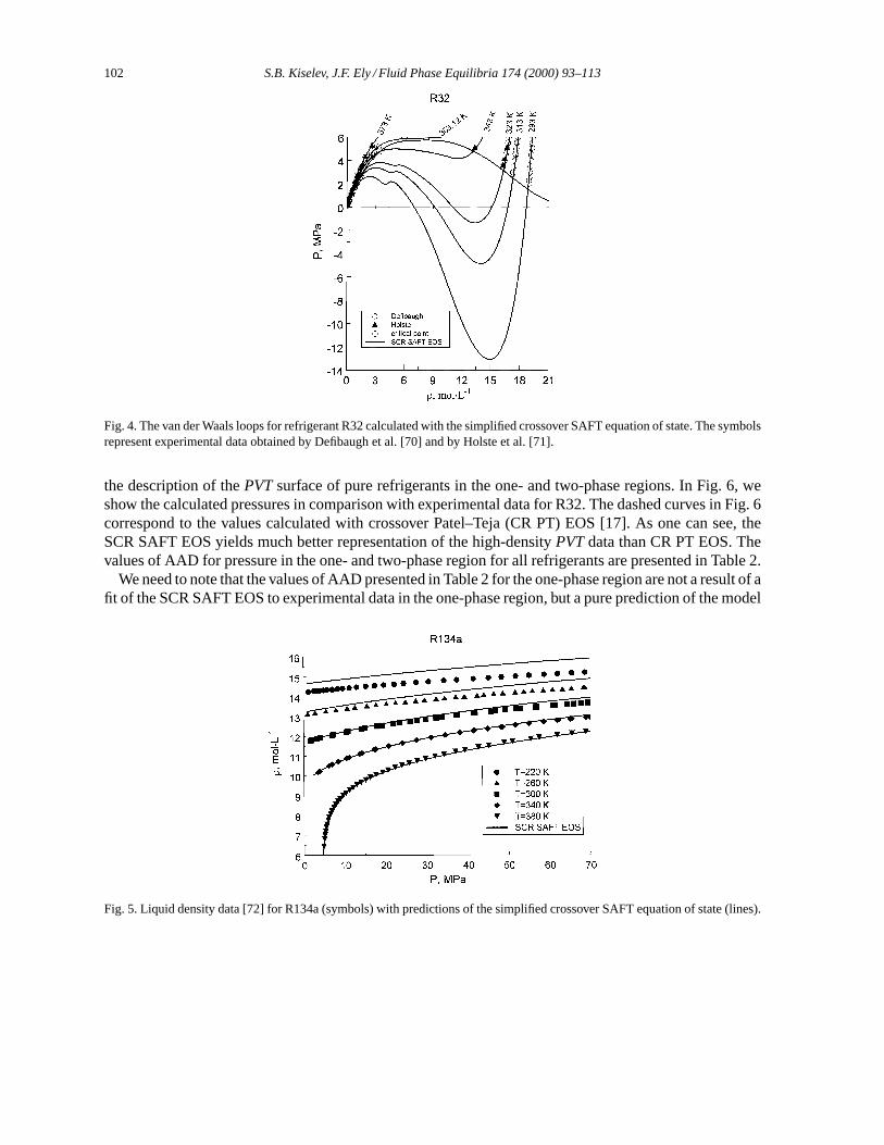
Since in the optimization of the model no experimental data in the one-phase region were used, itis interesting to test the predictions of the model in the one-phase region. A comparison of the calcu-lated liquid density with experimental data for R134a is shown in Fig. 5. The maximum deviation ofthe experimental densities from the calculated ones for all points presented in Fig. 6 does not exceed


Table 2System-dependent constants for the simplified crossover SAFT EOS

Parameter R12 R22 R32 R125 R134a R143a

v00 (mL.mol−1) 9.1736 6.4522 4.0768 5.7531 4.9959 6.1525m 4.2972 4.7746 5.6816 6.0515 6.5899 5.6319u0/k (K) 153.17 140.02 124.18 116.85 125.18 122.70Mw 120.91 86.469 52.024 120.00 102.03 84.044ω 0.177 0.221 0.277 0.303 0.327 0.261

Critical parametersa

T calcc (K) 385.40 368.94 351.50 339.67 374.72 346.47

Texp

c (K) 385.01 369.32 351.35 339.33 374.27 345.88ρcalc

c (mol.L−1) 4.7692 6.2044 8.3855 4.8398 5.0856 5.2505ρ

expc (mol.L−1) 4.6974 5.9559 8.2008 4.7600 5.1390 5.1282

P calcc (MPa) 4.0991 4.8245 5.7003 3.5961 4.0457 3.7812

Pexpc (MPa) 4.1290 4.9210 5.7950 3.6290 4.0650 3.7640

Average absolute deviation (AAD%)b

Psat 0.87 1.27 1.10 1.14 1.13 1.34ρL

sat 0.95 0.71 1.95 0.53 0.53 0.95PVT 2.88 1.99 2.09 2.24 1.84 2.48

a Superscripts “calc” and “exp” correspond to the calculated and experimental values, respectively. The experimental criticalparameters were taken from [31] for R12 and R22, from [33] for R32, R125 and R134a, and from [55] for R143a.

b AAD calculated in the temperature region 0.7T c ≤ T ≤ T c for Psat, at 0.5T c ≤ T ≤ T c for ρLsat, and in the one-phase

region atT ≥ T c andρ ≤ 2ρc for PVTdata.

0.6 mol l−1, or about 4%. These deviations are mostly observed at low temperatures viz.T ≤ 0.7T c,or u/kT ≥ 0.6. Since for simple non-associating fluids the SAFT EOS is simply a combination of therepulsive hard-sphere contribution and the dispersion term which is represented in the power series ofu/kT [34], it is not surprising that at lower temperatures whereu/kT ≈ 1 the crossover SAFT EOS gives

Fig. 1. Saturated pressure data for R12 [56–58], R22 [59,60], R32 [61], R125 [62], R134a [63], and R143a [64] (symbols) withpredictions of the simplified crossover SAFT equation of state (lines).


Fig. 2. Saturated density data for R12 [65], R22 [66], R32 [61], R125 [62,67,68], R134a [69], and R143a [64] (symbols) withpredictions of the simplified crossover SAFT equation of state (lines).

worse results than in the high-temperature region, atu/kT � 1. In order to improve the representation ofexperimental data with the crossover SAFT EOS in the regionu/kT ≈ 1, the original SAFT EOS shouldbe improved first. One way of doing this is to include into the original SAFT EOS the additional dipolarand quadrupolar contributions as was done, for example, in the BACKONE equations [45]. However,one should admit that even in the present form, the SCR SAFT EOS yields a major improvement in

Fig. 3. Percentage deviations of experimental saturated pressures (top) and saturated liquid densities (bottom) for pure refrigerantsfrom the values calculated with the simplified crossover SAFT equation of state. Legend as in Figs. 1 and 2.


Fig. 4. The van der Waals loops for refrigerant R32 calculated with the simplified crossover SAFT equation of state. The symbolsrepresent experimental data obtained by Defibaugh et al. [70] and by Holste et al. [71].

the description of thePVTsurface of pure refrigerants in the one- and two-phase regions. In Fig. 6, weshow the calculated pressures in comparison with experimental data for R32. The dashed curves in Fig. 6correspond to the values calculated with crossover Patel–Teja (CR PT) EOS [17]. As one can see, theSCR SAFT EOS yields much better representation of the high-densityPVTdata than CR PT EOS. Thevalues of AAD for pressure in the one- and two-phase region for all refrigerants are presented in Table 2.

We need to note that the values of AAD presented in Table 2 for the one-phase region are not a result of afit of the SCR SAFT EOS to experimental data in the one-phase region, but a pure prediction of the model

Fig. 5. Liquid density data [72] for R134a (symbols) with predictions of the simplified crossover SAFT equation of state (lines).


Fig. 6.PρT data [61,70,71] for R32 (symbols) with predictions of the simplified crossover SAFT equation of state (solid lines)and with the crossover cubic EOS [17] (dashed lines).


while for the energetic parameteru0(x), we adopt the van der Waals mixing rule:

u0(x) =∑

i

∑j

xixju0ij (29)

associated with the quadratic equation

u0ij =

√u0

i u0j (1 − kij ), kij = kji , kii = kjj = 0 (30)

wherekij is a binary interaction parameter. With these mixing rules, the critical parameters which appearin Eqs. (2)–(11) are not anymore the real critical parameters of a mixture which can be found from theconditions(

∂µ

∂x

)Pc,Tc(v=vc)

= 0,

(∂2µ

∂x2

)Pc,Tc(v=vc)

= 0 (31)

but the pseudo-critical parameters which are determined by Eqs. (14). This is a major simplification of themodel. The mixing rules as given by Eqs. (28)–(30) are simpler than those derived by Huang and Radosz[47,48] for the original SAFT EOS then the more rigorous critical region field-variable mixing rulesadopted in [26–30]. However, as we show below, using these simple mixing rules, the SCR SAFT EOSyields a satisfactory representation of the thermodynamic properties of mixtures of hydrofluorocarbonsin a large range of temperatures and densities.

We have chosen the refrigerant mixtures R22+ R12, R32+ R134a, and R125+ R32 for comparisonwith the model. The interaction parameters werek12 = 0.04 for R22+R12,k12 = 0.005 for R32+R134a,andk12 = 0.02 for the R125+R32 mixture. These values were obtained from a fit of the SCR SAFT EOSto the experimentalPVTxdata in the one-phase region obtained by Takaishi et al. [49] for the R22+ R12mixture and by Magee and Haynes [50] for R32+R134a and R125+R32 mixtures. A comparison of thecalculated values of pressure along isochores with experimental data of Takaishi et al. [49] is presented in

Fig. 7.PVTdata for the R22+R12 mixture obtained by Takaishi et al. [49] with predictions of the computer program CREOS97(dashed curves) and the simplified crossover SAFT equation of state (solid curves).


Fig. 8.PVTdata for R32+ R134a mixtures obtained by Magee and Haynes [50] (symbols) with predictions of the computerprogram CREOS97 (dashed curves) and the simplified crossover SAFT equation of state (solid curves).

Fig. 7. Figs. 8 and 9 compare the values obtained from our model with thePVTxdata of Magee and Haynes[50]. The dashed curves in all figures represent the values calculated with the parametric crossover model(computer program CREOS97) obtained in [31] for the R22+ R12 mixture and in [33] for R32+ R134aand R125+ R32 mixtures (Fig. 10). The SCR SAFT model shows good agreement for all mixtures. Themaximum deviation of the calculated values of pressure from the experimental ones does not exceed 2%.

Fig. 9. PVT data for R125+ R32 mixtures obtained by Magee and Haynes [50] (symbols) with predictions of the computerprogram CREOS97 (dashed curves) and the simplified crossover SAFT equation of state (solid curves).


Fig. 10.PVT data for R32+ R134a mixtures obtained by Fukushima and co-workers [51] (symbols) with predictions of thecomputer program CREOS97 (dashed curves) and the simplified crossover SAFT equation of state (solid curves).

Only for the R22+ R12 mixture along the isochoreρ = 7.118 mol.L−1, systematic deviations up to 4%are observed.

In Fig. 9, we compare the predictions of the model forPVTx properties for a 45.67 mol% R32+54.33 mol% R134a system with the experimental data of Fukushima et al. [51]. The data are over a widerange of temperatures from 314 to 424 K and at pressures from 1.5 to 10.1 MPa, and densities over therangeρ = 0.902–10.033 mol l−1. Since these data were not used for the optimization of the model,this is a good test of the predictability of the model. The SCR SAFT EOS shows good agreement withthe data, while the parametric crossover model gives systematic deviation from the experimental dataat isochoresρ = 0.902 and 1.236 mol l−1. This deviation is a direct consequence of the fact that theparametric crossover model fails to reproduce the ideal gas limit.

Even though the parameters forkij were found using one-phase data, the SCR SAFT EOS can beextrapolated into the two-phase region. Figs. 11–14 show the VLE coexistence curves for R22+ R12,R32+R134a, and R125+R32 mixtures in the critical region and below. The model agrees very well withthe data up to temperaturesT = 0.99T c(x). For calculations of the VLE properties of the mixtures, weused an iterative algorithm developed by Lemmon [52]. As was also pointed out in [18], this algorithmdoes not converge very close to the critical point of a mixture, at|τ(x)| ≤ 10−2, and alternative algorithmsshould be used. For comparison, we also have shown the predictions from the parametric crossover modelCREOS97 [33] and NIST REFPROP [53]. As one can see, far from the critical point, all models givepractically identical results which are in good agreement with experimental data. However, as the criticalpoint approaches the NIST REFPROP, predictions become less accurate and exhibit systematic deviationsfrom experimental data, while the SCR SAFT EOS yields a reasonably good description of experimental


Fig. 11. Dew-bubble curves for R22+ R12 mixtures. The symbols indicate experimental data obtained by obtained by Takaishiet al. [49], and the curves represent predictions from the computer program CREOS97 (dashed curves) and the simplifiedcrossover SAFT equation of state (solid curves).

data up toT = 0.99T c(x). Fig. 15 shows the experimental VLE data for R125+ R32 mixtures obtainedby Higashi [54] at four isotherms far from the critical point with the predictions of the SCR SAFT EOS,the parametric crossover model CREOS97 [33], and NIST REFPROP [53]. Quantitatively, all modelsgive similar predictions which are in good agreement with experimental data; however, qualitatively,

Fig. 12. VLE data for R22+ R12 mixtures obtained by Takaishi et al. [49] (symbols) with predictions of the computer programCREOS97 (dashed curves) and the simplified crossover SAFT equation of state (solid curves).


Fig. 13. VLE data for R32+ R134a mixtures of Higashi [73] and of Fukushima [74] at two concentrations of R134a andpredictions from the computer program NIST REFPROP [53], the computer program CREOS97 (dashed curves), and of thesimplified crossover SAFT model (solid curves).

Fig. 14. VLE data for R125+ R32 mixtures of Higashi [54] at two concentrations of R32 and predictions from the computerprogram NIST REFPROP [53], the computer program CREOS97 (dashed curves), and of the simplified crossover SAFT model(solid curves).


Fig. 15. The pressure–composition diagram for R125+ R32 mixtures. The symbols indicate experimental data obtained byHigashi [54] at four temperatures, and the curves represent predictions from the computer program CREOS97 (dashed curves),the computer program NIST REFPROP [53] (dashed–dotted curves), and of the simplified crossover SAFT model (solid curves).

the results are different. Experimental data obtained by Higashi for R125+ R32 mixtures [54] exhibitthe appearance of an azeotrope at approximately 90 mol% R32 at temperatures less thanT = 303 K.The SCR SAFT model predicts the appearance of an azeotrope atT ≤ 283 K, the computer programCREOS97 predicts an azeotrope at temperaturesT ≥ 303K. The newest version of NIST REFPROP[75,76] predicts a very weak azeotrope for R125+R32 mixtures atP=0.1–0.4 MPa at compositions ofabout 0.9 mole fraction R32. ByP=1 MPA, the azeotrope disappears. We cannot say for sure whichprediction is correct. In order to answer this question, more experimental information for this mixture isneeded.

5. Conclusions

On the basis of the crossover SAFT EOS obtained before [19], we develop a simplified crossovermodification of the SAFT equation of state which, similar to the original SAFT EOS, contains onlythree adjustable parameters but gives an accurate prediction of the critical parameters for pure fluids andyields a much better representation of thePVTand VLE properties pure fluids in and beyond the criticalregion than original SAFT EOS and CR PT EOS [17]. Unlike our previous crossover EOS based on thelinear model EOS for the parametric variableq [17,19], the SCR SAFT EOS based on the parametricsine model [41] can be extended into the metastable region and represents analytically connected vander Waals loops. In the present work, we tested the SCR SAFT EOS experimental data again for purerefrigerants in the one- and two-phase regions. Good agreement with experimentalPVTand VLE datawas achieved in the wide rage of the parameters of state including the critical region.

In order to extend the crossover SAFT EOS to mixtures, we formulate the simple mixing rules for thesystem-dependent parameters of the model in terms of composition. Although with these simplified mix-ing rules the crossover SAFT EOS does not reproduce some of the known scaling laws in the asymptotic


critical region of mixtures, at dimensionless temperatures|τ(x)| ≥ 10−2, it yields an accurate represen-tation of the thermodynamic surface of the mixtures of hydrofluorocarbons in the one- and two-phaseregions. To extend the obtained results to other, more complex fluids and their mixtures, the model shouldbe checked with other mixing rules, with a more rigorous theoretical basis.

List of symbolsa Helmholtz free energy per mole (total, res, assoc, etc.)a2i coefficients in the kernel term (i = 0 andi = 1)A dimensionless Helmholtz free energy (total, res, etc.)b2 universal linear-model parameterC integration constant in Eq. (6)d1 rectilinear diameter amplituded

(j)

1 constants in Eq. (26)(j = 0, 1)

Dij universal constants in Eq. (4)e/k constant in Eq. (7) (K)ghs hard sphere radial distribution functionGi Ginzburg number1η order parameterk Boltzmann’s constant≈ 1.3814× 10−23 J/Kkij binary interaction parameterK kernel termm number of segmentsm0 sine-model critical amplitudeMw molecular weightN total number of moleculesp2 universal sine-model parameterP pressurePc critical pressureq argument of crossover functionr parametric variableR gas constantT temperature (K)Tc critical temperature (K)1T dimensionless deviation of the temperature from the classical critical temperatureu/k temperature-dependent dispersion energy of interaction between segments (K)u0/k temperature-independent dispersion energy of interaction between segments (K)v molar volumev1 system-dependent coefficient in Eq. (21)v

(j)

1 coefficients in Eq. (25)(j = 0, 1)

v0 temperature-dependent segment volumev00 temperature-independent segment volume1v classical order parameter1vc shift of the critical volume


V total volumex composition of a mixtureY crossover function

Greek lettersα universal critical exponentβ universal critical exponentδ1 universal constant in Eq. (21)δτ constant in Eq. (23)δρ constant in Eq. (24)1η re-scaled order parameter1ηc dimensionless shift of the critical volume1 difference11 universal critical exponentγ universal critical exponentµ chemical potential of a mixtureτ reduced temperature difference1τ c dimensionless shift of the critical temperatureτ re-scaled reduced temperature differenceθ parametric variableρ molar densityρc critical density (mol/l)

Superscriptsassoc associationG gasideal ideal gasL liquidres residual

Subscriptsc criticalsat saturated0 classical

Acknowledgements

The authors are indebted to M. Fisher for providing us with the manuscript of his paper prior to publi-cation. The research was supported by the US Department of Energy, Office of Basic Energy Sciences,under Grant No. DE-FG03-95ER41568.

References

[1] J.V. Sengers, J.M.H. Levelt Sengers, Annu. Rev. Phys. Chem. 37 (1986) 189.


[2] M.A. Anisimov, S.B. Kiselev, in: A.E. Scheindlin, V.E. Fortov (Eds.), Sov. Tech. Rev. B. Therm. Phys., Vol. 3, Part 2,Harwood, New York, 1992, pp. 1–121.

[3] J.R. Fox, Fluid Phase Equilibria 14 (1983) 45.[4] A. Parola, L. Reatto, Phys. Rev. A 31 (1985) 3309.[5] M. Tau, A. Parola, D. Pini, L. Reatto, Phys. Rev. E 52 (1995) 2644.[6] L. Reatto, A. Parola, J. Phys.: Condens. Matter 8 (1996) 9221.[7] L. Lue, J.M. Praustitz, AIChE J. 44 (1998) 1455.[8] J.A. White, Fluid Phase Equilibria 75 (1992) 53.[9] J.A. White, S. Zhang, J. Chem. Phys. 99 (1993) 2012.

[10] J.A. White, S. Zhang, J. Chem. Phys. 103 (1995) 1922.[11] J.A. White, J. Chem. Phys. 111 (1999) 9352.[12] J.A. White, J. Chem. Phys. 112 (2000) 3236.[13] T. Kraska, U.K. Deiters, Int. J. Thermophys. 15 (1993) 261.[14] K. Leonhard, T. Kraska, J. Supercritical Fluids 16 (1999) 1.[15] Y. Tang, J. Chem. Phys. 109 (1998) 5935.[16] F. Fornasiero, L. Lue, A. Bertucco, AIChE J. 45 (1999) 906.[17] S.B. Kiselev, Fluid Phase Equilibria 147 (1998) 7.[18] S.B. Kiselev, D.G. Friend, Fluid Phase Equilibria 162 (1999) 51.[19] S.B. Kiselev, J.F. Ely, Ind. Eng. Chem. Res. 38 (1999) 4993.[20] A. Jiang, J.M. Praustitz, J. Chem. Phys. 111 (1999) 5964.[21] M.E. Fisher, Phys. Rev. 176 (1968) 257.[22] R.B. Griffiths, J.C. Wheeler, Phys. Rev. A 2 (1970) 1047.[23] W.F. Saam, Phys. Rev. A 2 (1970) 1461.[24] M.A. Anisimov, A.V. Voronel, E.E. Gorodetskii, Sov. Phys. JETP 33 (1971) 605.[25] S.B. Kiselev, High Temp. 26 (1988) 337.[26] G.X. Jin, S. Tang, J.V. Sengers, Phys. Rev. E 47 (1993) 388.[27] A.A. Povodyrev, G.X. Jin, S.B. Kiselev, J.V. Sengers, Int. J. Thermophys. 17 (1996) 909.[28] M.Y. Belyakov, S.B. Kiselev, J.C. Rainwater, J. Chem. Phys. 107 (1997) 3085.[29] S.B. Kiselev, Fluid Phase Equilibria 128 (1997) 1.[30] S.B. Kiselev, J.C. Rainwater, Fluid Phase Equilibria 141 (1997) 129.[31] S.B. Kiselev, J.C. Rainwater, M.L. Huber, Fluid Phase Equilibria 150/151 (1998) 469.[32] S.B. Kiselev, J.C. Rainwater, J. Chem. Phys. 109 (1998) 643.[33] S.B. Kiselev, M.L. Huber, Int. J. Refrig. 21 (1998) 64.[34] H.S. Huang, M. Radosz, Ind. Eng. Chem. Res. 29 (1990) 2284.[35] B.J. Alder, D.A. Young, M.A. Mark, J. Chem. Phys. 56 (1972) 3013.[36] S.B. Kiselev, J.F. Ely, H. Adidharma, M. Radosz, Fluid Phase Equilibria, in press.[37] S.B. Kiselev, D.G. Friend, Fluid Phase Equilibria 155 (1999) 33.[38] M.Y. Belyakov, S.B. Kiselev, Physica A 190 (1992) 75.[39] M.A. Anisimov, S.B. Kiselev, J.V. Sengers, S. Tang, Physica A 188 (1992) 487.[40] A. Berestov, Sov. Phys. JETP 72 (1977) 338.[41] M.E. Fisher, S.-Y. Zinn, P.J. Upton, Phys. Rev. B 59 (1999) 14533.[42] P. Schofield, Phys. Rev. Lett. 22 (1969) 606.[43] P. Schofield, J.D. Litster, J.T. Ho, Phys. Rev. Lett. 23 (1969) 1098.[44] S.B. Kiselev, High Temp. 28 (1988) 42.[45] S. Calero, M. Wendland, J. Fischer, Fluid Phase Equilibria 152 (1998) 1.[46] M. Fermeglia, A. Bertucco, D. Patrizio, Chem. Eng. Sci. 52 (1997) 1517.[47] H.S. Huang, M. Radosz, Ind. Eng. Chem. Res. 30 (1991) 1994.[48] H.S. Huang, M. Radosz, Fluid Phase Equilibria 70 (1991) 33.[49] Y. Takaishi, N. Kagawa, M. Uematsu, K. Watanabe, in: J.V. Sengers (Ed.), Proceedings of the 8th Symposium on Thermal

Propulsion, Vol. 2, ASME, Gaithersburg, MD, 1982, pp. 387–395.[50] J.W. Magee, W.M. Haynes, Int. J. Thermophys. 21 (2000) 113.


[51] M. Fukushima, K. Machidori, S. Kumano, S. Ohotoshi, in: Proceedings of the 14th Japan Symposium on ThermophysicalProperties, Japan Society of Thermophysical Properties, Yokohama, Japan, 1993, pp. 275–278.

[52] E.W. Lemmon, A generalized model for the prediction of the thermodynamic properties of mixtures including vapor–liquidequilibrium, Ph.D. Thesis, University of Idaho, Moscow, ID, 1996.

[53] NIST Thermodynamic Properties of Refrigerant Mixtures Database, NIST REFPROP, v5.12, Natl. Inst. Stand. Technol.,Gaitherburg, MD, 1987.

[54] Y. Higashi, in: Proceedings of the 19th International Congress on Refrigeration, Vol. IVa, International Institute ofRefrigeration, The Hague, The Netherlands, 1995, pp. 297–305.

[55] Y. Higashi, T. Ikeda, Fluid Phase Equilibria 125 (1996) 139.[56] L.F. Kells, S.R. Orfeo, W.H. Mears, Refrig. Eng. 63 (1955) 46.[57] K. Watanabe, T. Tanaka, K. Oguchi, in: A. Cezarliyan (Ed.), Proceedings of the 7th ASME Thermal Propulsion Conference,

ASME, Gaithersburg, MD, 1977, pp. 470–479.[58] E. Fernandez-Fassnacht, F. Del Rio, Cryogenics 25 (1985) 204.[59] M. Zander, in: J. Moszynski (Ed.), Proceedings of the 4th ASME Thermophysics Symposium, ASME, Gaithersburg, MD,

1968, pp. 114–123.[60] L.M. Lagutina, Kholodilnaya Tekhnika (Russian) 43 (1966) 25.[61] P.F. Malbrunot, P.A. Meunier, G.M. Scatena, W.H. Mears, K.P. Murphy, J.V. Sinka, J. Chem. Eng. Data 13 (1968) 16.[62] J.W. Magee, Int. J. Thermophys. 17 (1996) 803.[63] H.D. Baehr, R. Tillner-Roth, J. Chem. Thermodyn. 23 (1991) 1063.[64] M. McLinden, private communication, Div. 838.08, NIST, Boulder, CO, 1980.[65] R.C. McHarness, B.J. Eiseman, J.J. Martin, Refrig. Eng. 63 (1955) 31.[66] M. Okada, M. Uematsu, K. Watanabe, J. Chem. Thermodyn. 18 (1986) 527.[67] D.R. Defibaugh, G. Morrison, Fluid Phase Equilibria 80 (1992) 157.[68] S. Kuwubara, H. Aoyama, H. Sato, K. Watanabe, J. Chem. Eng. Data 40 (1995) 112.[69] G. Morrison, D.K. Ward, Fluid Phase Equilibria 62 (1991) 65.[70] D.R. Defibaugh, G. Morrison, L.A. Weber, J. Chem. Eng. Data 39 (1994) 333.[71] J.C. Holste, H.A. Duarte-Garza, M.A. Villamanan-Olfos, in: Proceedings of the 1993 ASME Winter Annual Meeting, Paper

No. 93-WA/HT-60, ASME, New Orleans, 1993.[72] H. Hou, J.C. Holste, B.E. Gammon, K.N. Marsh, Int. J. Refrig. 15 (1992) 365.[73] Y. Higashi, Int. J. Thermophys. 16 (1995) 1175.[74] M. Fukushima, Trans. Jpn. Assoc. Refrig. 7 (1990) 243.[75] NIST Thermodynamic and Transport properties of Refrigerants and Refrigerant Mixtures, NIST REFPROP, V6.01, Natl.

Inst. Stand. Technol., Gaitherburg, MD, 1998.[76] E.W. Lemmon, R.T. Jacobsen, Int. J. Thermophys. 20 (1999) 1629.

Simplified crossover SAFT equation of state for pure fluids and fluid

Documents

Transcript of Simplified crossover SAFT equation of state for pure fluids and fluid