Simplified Analysis of IMU Sensor Corruptions on Existing ...
87
Simplified Analysis of IMU Sensor Corruptions on Existing Pendulation Control System For Ship-Mounted Crane Jia Qi “Josh” Zhou Thesis submitted to the Faculty of the Virginia Polytechnic Institute and State University in partial fulfillment of the requirements for the degree of Master of Science in Aerospace Engineering Dr. Hanspeter Schaub, Committee Chair Dr. Christopher Hall, Committee Member Dr. Craig Woolsey, Comittee Member December 12, 2006 Blacksburg, Virginia Keywords: Ship Crane, Motion Sensing, Pendulation Control, Sensor Corruption Copyright 2006, Jia Qi “Josh” Zhou
Transcript of Simplified Analysis of IMU Sensor Corruptions on Existing ...

Simplified Analysis of IMU Sensor Corruptions on Existing
Pendulation Control System For Ship-Mounted Crane
Jia Qi “Josh” Zhou
Thesis submitted to the Faculty of the
Virginia Polytechnic Institute and State University
in partial fulfillment of the requirements for the degree of
Master of Science
in
Aerospace Engineering
Dr. Hanspeter Schaub, Committee Chair
Dr. Christopher Hall, Committee Member
Dr. Craig Woolsey, Comittee Member
December 12, 2006
Blacksburg, Virginia
Keywords: Ship Crane, Motion Sensing, Pendulation Control, Sensor Corruption
Copyright 2006, Jia Qi “Josh” Zhou

SIMPLIFIED ANALYSIS OF IMU SENSOR CORRUPTIONS ON
EXISTING PENDULATION CONTROL SYSTEM FOR
SHIP-MOUNTED CRANE
Jia Qi “Josh” Zhou
(ABSTRACT)
Ship-mounted boom cranes play an important role in the ship-to-ship offshore cargo trans-
port process. In recent years, there has been significant need to increase stability of the
payload during the cargo transport process for both safety and efficiency reasons. However,
the stability of the payload during the transport process directly correlates to the ship’s
pitch and roll motion that in turn relates to the current particular sea-state.
In this study, we analyze an existing Pendulation Control System (PCS) developed by Sandia
National Laboratories that reduces the payload’s pendulation movement during transport.
This system measures the ship motion through a complex inertial navigation system using
an IMU and dual GPS receivers. In trying to simplify the analysis of the IMU sensor,
we simulate new control solutions based solely on an IMU-only ship motion measurement
system using both position- and velocity-based controllers. This study shows that an optional
bandpass filter in the new control solution can reject a bias that appears in the estimated
accelerometer data at the expense of higher sensitivity for the control. This study also shows
that the velocity-based solution provides comparable if not better results than the position-
based solution. Both methods are sensitive to the difference between the ship motion period
and the center frequency of its bandpass filter. Lastly, it is shown that the bias of an
accelerometer is not a large source of payload disturbance as compared to the scale factor
error.
This work received support from the Naval Surface Warfare Center, Carderock, MD.

Acknowledgments
I would first like to express my sincere gratitude to my advisor, Dr. Hanspeter Schaub,
for providing me the opportunity to work with him. Your assistance and support for me on
this project were invaluable. I thank you for the patience you have shown me and putting
up with me through everything. These qualities of yours will forever be appreciated. I would
also like to thank Dr. Christopher Hall and Dr. Craig Woolsey for their time and effort for
being on my committee. I enjoyed my time in both of your classes. I want to thank my fellow
research group members, Chris Romanelli and John Berryman, for their assistance in my
debugging process. I will always be forever thankful to my parents for making the sacrifices
in their lives to bring me out to the United States so that I could have the opportunity to
grow and a chance for a better life. Their constant love and support helped me in part to
become the person I am today. Lastly, I would just like to thank all my dear friends past
and present for your friendship and support. My life just would not be the same without
each and every one of you.
iii
Contents
1 Introduction 1
1.1 Motivation . . . . . . . . . . . . . . . . . . . . . . . . . . . . . . . . . . . . . 3
1.2 Problem Definition . . . . . . . . . . . . . . . . . . . . . . . . . . . . . . . . 5
1.3 Approach . . . . . . . . . . . . . . . . . . . . . . . . . . . . . . . . . . . . . 7
1.4 Overview . . . . . . . . . . . . . . . . . . . . . . . . . . . . . . . . . . . . . . 8
2 Literature Review 9
2.1 Relevant History . . . . . . . . . . . . . . . . . . . . . . . . . . . . . . . . . 9
2.2 Alternate Solutions . . . . . . . . . . . . . . . . . . . . . . . . . . . . . . . . 11
2.3 Summary . . . . . . . . . . . . . . . . . . . . . . . . . . . . . . . . . . . . . 13
3 Sensor Details 14
3.1 How IMUs Operate . . . . . . . . . . . . . . . . . . . . . . . . . . . . . . . . 14
3.2 Types of IMU Corruptions . . . . . . . . . . . . . . . . . . . . . . . . . . . . 15
3.2.1 Scale Factor . . . . . . . . . . . . . . . . . . . . . . . . . . . . . . . . 15
3.2.2 Bias . . . . . . . . . . . . . . . . . . . . . . . . . . . . . . . . . . . . 16
iv

3.2.3 Random Drift . . . . . . . . . . . . . . . . . . . . . . . . . . . . . . . 17
3.2.4 White Noise . . . . . . . . . . . . . . . . . . . . . . . . . . . . . . . . 17
3.2.5 Other Errors . . . . . . . . . . . . . . . . . . . . . . . . . . . . . . . 18
3.3 Types of IMU Sensors and Cost . . . . . . . . . . . . . . . . . . . . . . . . . 18
3.4 Summary . . . . . . . . . . . . . . . . . . . . . . . . . . . . . . . . . . . . . 20
4 Relevant Concepts 21
4.1 Slow Drifting Frame . . . . . . . . . . . . . . . . . . . . . . . . . . . . . . . 21
4.2 Crane Kinematics . . . . . . . . . . . . . . . . . . . . . . . . . . . . . . . . . 23
4.3 Digital Filtering of Ship Motion Sensing . . . . . . . . . . . . . . . . . . . . 27
4.3.1 Advantages of Digital Filters . . . . . . . . . . . . . . . . . . . . . . . 27
4.3.2 Application . . . . . . . . . . . . . . . . . . . . . . . . . . . . . . . . 27
4.3.3 Filter Types . . . . . . . . . . . . . . . . . . . . . . . . . . . . . . . . 28
4.3.4 Filter Selection and Algorithm . . . . . . . . . . . . . . . . . . . . . . 29
4.3.5 Filter Behaviors on POS/MV Based Control . . . . . . . . . . . . . . 30
4.3.6 Filter Behaviors on IMU-Based Control . . . . . . . . . . . . . . . . . 31
4.4 Summary . . . . . . . . . . . . . . . . . . . . . . . . . . . . . . . . . . . . . 34
5 Differences Between Control Solutions 35
5.1 3D Inverse Kinematics . . . . . . . . . . . . . . . . . . . . . . . . . . . . . . 35
5.1.1 3D Inverse Kinematics of Position Based Control . . . . . . . . . . . 36
5.1.2 3D Inverse Kinematics of Velocity Based Control w/ IMU . . . . . . 38
v

5.2 Simplifying from 3D to 1D . . . . . . . . . . . . . . . . . . . . . . . . . . . . 40
5.3 Equations of Motion . . . . . . . . . . . . . . . . . . . . . . . . . . . . . . . 42
5.3.1 Derivation Using Lagrange’s Equation . . . . . . . . . . . . . . . . . 42
5.3.2 Applying Lagrange’s Equation to the 1-D Cart Pendulum . . . . . . . 43
5.3.3 Solving the Equations of Motion . . . . . . . . . . . . . . . . . . . . . 44
5.4 Simplified 1D Control Using Position Based Inverse Kinematics . . . . . . . 45
5.5 Simplified 1D Control Using Velocity Based Inverse Kinematics . . . . . . . 48
5.6 Summary . . . . . . . . . . . . . . . . . . . . . . . . . . . . . . . . . . . . . 49
6 Results 50
6.1 Applying the Optional Filter . . . . . . . . . . . . . . . . . . . . . . . . . . . 50
6.2 Sweeps When Varying Different IMU Sensor Parameters . . . . . . . . . . . 54
6.3 Summary . . . . . . . . . . . . . . . . . . . . . . . . . . . . . . . . . . . . . 62
7 Conclusion 63
Bibliography 65
A MATLAB Codes 68
A.1 Main Program . . . . . . . . . . . . . . . . . . . . . . . . . . . . . . . . . . . 68
A.2 Function Files . . . . . . . . . . . . . . . . . . . . . . . . . . . . . . . . . . . 74
vi

List of Figures
1.1 An example of a gantry crane [5] . . . . . . . . . . . . . . . . . . . . . . . . 2
1.2 An example of a rotary crane [5] . . . . . . . . . . . . . . . . . . . . . . . . . 2
1.3 An example of boom cranes onboard a crane ship [6] . . . . . . . . . . . . . 3
1.4 Crane ship during cargo transfer [7] . . . . . . . . . . . . . . . . . . . . . . . 4
1.5 Crane System with slew angle α, luff angle β, hoist length Lh . . . . . . . . 5
1.6 Using cart pendulum to model the rolling motion of the ship . . . . . . . . . 7
2.1 An example of a Rider-Block-Tagline-System [8] . . . . . . . . . . . . . . . . 10
3.1 Example of a scale factor error . . . . . . . . . . . . . . . . . . . . . . . . . . 16
3.2 Example of a bias . . . . . . . . . . . . . . . . . . . . . . . . . . . . . . . . . 17
3.3 Example of white noise corruption . . . . . . . . . . . . . . . . . . . . . . . . 18
3.4 Existing GPS/IMU system, POS/MV 320 [25] . . . . . . . . . . . . . . . . . 19
4.1 Example of the slow drifting reference frame I ′ . . . . . . . . . . . . . . . . 22
4.2 Top view showing crane frame and slew angle, α . . . . . . . . . . . . . . . . 23
4.3 Side view showing crane frame and luff angle, β . . . . . . . . . . . . . . . . 24
vii

4.4 Inertial, Ship Sensor, and Crane Coordinate Frames . . . . . . . . . . . . . . 25
4.5 Filtering Process of POS/MV Based Control . . . . . . . . . . . . . . . . . . 31
4.6 Error signals on a)Calm Day, b)Medium Day, c)Rough Day . . . . . . . . . . 32
4.7 Comparison of True, Sensed, and Filtered Position of POS/MV Based Control 33
4.8 Filtering Process of IMU Based Control . . . . . . . . . . . . . . . . . . . . . 33
5.1 Diagram of 1-D Cart Pendulum . . . . . . . . . . . . . . . . . . . . . . . . . 41
5.2 Flowchart of the Rate-Based Position Control . . . . . . . . . . . . . . . . . 45
5.3 Flowchart of the Rate-Based Velocity Control . . . . . . . . . . . . . . . . . 49
6.1 Effects of Filtering Without Additional Filter in IMU-Based Control . . . . . 51
6.2 Effects of Filtering With Additional Filter in IMU-Based Control . . . . . . 52
6.3 Effect of Optional Bandpass Filter in Rate-based Position Control . . . . . . 53
6.4 Effect of Optional Bandpass Filter in Rate-based Velocity Control . . . . . . 53
6.5 Ship Rolling Angle vs Horizontal Boomtip Motion with Varying Luff Angle . 56
6.6 Ship Motion Amplitude vs Ship Motion Period for a)Position and b)Velocity-
Based PCS with Expensive IMU and Filter On . . . . . . . . . . . . . . . . 57
6.7 Ship Motion Amplitude vs Ship Motion Period for a)Position and b)Velocity-
Based PCS with Cheaper IMU and Filter On . . . . . . . . . . . . . . . . . 57
6.8 Ship Motion Amplitude vs Ship Motion Period for a)Position and b)Velocity-
Based PCS with Expensive IMU and Filter Off . . . . . . . . . . . . . . . . 58
6.9 Ship Motion Amplitude vs Ship Motion Period for a)Position and b)Velocity-
Based PCS with Cheaper IMU and Filter Off . . . . . . . . . . . . . . . . . 58
viii

6.10 Filter center frequency vs Ship Motion Period for a)Position and b)Velocity-
Based PCS . . . . . . . . . . . . . . . . . . . . . . . . . . . . . . . . . . . . 59
6.11 Cart Pendulum Sweep Analysis of Scale Factor vs Bias in Position-based Con-
trol with Optional Bandpass Filter a)Off, b)On . . . . . . . . . . . . . . . . 61
6.12 Cart Pendulum Sweep Analysis of Scale Factor vs Bias Velocity-based Control
with Optional Bandpass Filter a)Off, b)On . . . . . . . . . . . . . . . . . . . 61
ix

List of Tables
3.1 Listing of IMU, errors and estimated cost. . . . . . . . . . . . . . . . . . . . 20
6.1 List of Parameters Used in Cart-Pendulum Simulation . . . . . . . . . . . . 55
x

List of Abbreviations
COTS Container Off-loading and Transfer System
GPS Global Positioning System
IMU Inertial Measurement Unit
MSA Micromachined Silicon Accelerometer
PCS Pendulation Control System
RTBS Rider Block Tagline System
T-ACS Tactical Auxilary Crane Ship
xi

Chapter 1
Introduction
Cranes apply the concept of simple machines to help humans alleviate the rigors of carrying
heavy loads from one place to another. They have been in use for many centuries by numerous
civilizations. During ancient times, a sign of a civilization’s prosperity is often reflected by
the sheer magnitude of its monuments, temples, and other prominent structures, for which
cranes had a big part in their constructions. In the current age of global economy, one telling
sign of a nation’s prosperity is often reflected in the amount of goods that are imported and
exported. Once again, cranes play a big part when it comes to loading and offloading
operations between ship-to-ship, ship-to-shore, and vice versa.
There are generally three common types of cranes. Their differences reside in the way the
cranes are supported. A gantry crane seen in Figure 1.1 has a trolley moving over a girder.
This type of crane is generally seen in construction sites, steel mills, assembly lines, and
docks of various ports because of its usefulness in moving cargo from one point on land to
another. The second type of crane seen in Figure 1.2 is the rotary crane. The rotary crane
rotates horizontally about a fixed vertical axis and provides both a translation and a rotation
movement. Rotary cranes are generally seen on building construction sites. The third type of
crane, which features the main object of this report, is the boom crane. As seen in Figure 1.3,
1

Chapter 1. Introduction 2
Figure 1.1: An example of a gantry crane [5]
Figure 1.2: An example of a rotary crane [5]

Chapter 1. Introduction 3
the boom tip provides the suspension point for payloads. This design provides rotations in
the horizontal plane as well as the vertical plane. The boom crane is advantageous over
the other two types of cranes because the boom support loads in compression as opposed to
bending. That is why in areas where space is not readily available, the presence of boom
cranes are common. These places include onboard ships, certain construction sites, as well
as vehicles for ease of mobility.
Figure 1.3: An example of boom cranes onboard a crane ship [6]
1.1 Motivation
The military has had a lot of interest when it comes to the safeguard of its supplies during
transport. To ensure flexibility and expedience, the U.S. Navy employs a fleet of crane ships
used to offload containers between ships as a part of the Container Off-loading and Transfer
System (COTS). These ships are especially useful in places where off-shore loading facilities
are not available or are inadequate. Typically, these Tactical Auxiliary Crane Ships (T-ACS)
anchor off the coast, then a larger cargo vessel and a lighter landing vessel each dock beside
the crane ship as shown in Figure 1.4. A crane operator adjusts the combination of crane’s

Chapter 1. Introduction 4
Figure 1.4: Crane ship during cargo transfer [7]
hoist length, luff, and slew states (see Figure 1.5) to move the container from the cargo
vessel to the lighter vessel. In the process, the cargo container passes over the decks of all
the ships involved, as well as some of its personnel. If the payload swing is not excessive,
then the transport process should be a smooth one. However, it has been shown by Vaughers
and Mardiros [1] that even under sea-state level three (according to the Pierson-Moskowitz
Sea Spectrum with significant wave heights in the range of 1.0 – 1.6 m), the crane payload
can produce dangerous amounts of pendulation swing onboard the auxiliary crane ships.
Uncontrolled pendulation swing increases the risk of possible damage to the cargo, the ships
involved, and their personnel. Generally, the Navy suspends transport operations at a Sea
State level of greater than two.
The operation limitation caused by Sea State of level three prompted the development of
the Pendulation Control System (PCS) by Robinett, et al. [2] of Sandia National Laboratories
and was installed in the fall of 2002 onboard the T-ACS 5 vessel the Flickertail State (the
ship seen in Figure 1.3). Its goal was to reduce the payload pendulation and allow for safer
operation of ship cranes under more severe sea-states, and thereby reduce the time and

Chapter 1. Introduction 5
Figure 1.5: Crane System with slew angle α, luff angle β, hoist length Lh
monetary cost for the Navy. The implemented PCS showed improvement in performance as
cargo transfers were able to be completed at higher ship roll angles. The improvement was
the result of comparing data from the PCS against data from existing crane control modes
from cranes with both RBTS (Rider Block Tagline System) and non-RBTS systems [3].
A newly proposed upgrade to the PCS involves changing its algorithm to use the ship’s
velocity data instead of its position data. This new rate-based control relies on the ship’s
measured angular rates and translational acceleration from the rate gyro and accelerometer
components of an IMU. More specifically, sensor information needed are the angular rate ω,
the acceleration g, the roll angle φ, and pitch angle θ. One clear benefit of the rate-based
control solution is the significant cost reduction in terms of moving from a fully integrated
GPS/IMU navigation system to an IMU-only system.
1.2 Problem Definition
The three primary sources of payload swing excitation are operator commands, sea-induced
motion, and external disburbances. To counter the sea-induced motion, various types of
sensors are incorporated in control solutions to ease operator’s workload and limit the swing.
Subsequently, there are three types of sensors that are used to keep track of various states

Chapter 1. Introduction 6
of the payload at any given time. They are the inertial measurement unit (IMU), the
operator, and the swing sensors. This report focuses in on the IMU as it is assumed the
swing sensors provide accurate results. The current prototype pendulation control system
used to stabilize payload during transport process uses a GPS/IMU based system to sense
the crane ship position and motion. In order for the crane operator to move the payload in
a safe and swing-free maneuver, the GPS/IMU must have a high accuracy to compensate
for the motion of the occasional rough sea conditions. Higher accuracy translates into a
very high sensor cost for the Navy for each PCS installation. As with any other sensor, the
GPS is prone to different biases, noises, and other disturbances. It has been shown that the
GPS tends to show more deviations at higher latitudes due to scintillation effects caused by
disturbances in Earth’s ionosphere [4]. All of these variables are sources for errors that cause
inaccurate sensing during a payload transfer, resulting in longer operation times.
When referring to the new rate-based control method, one must realize that an IMU will
experience corruptions. In order to make a numerical simulation as real as possible, the es-
timator that processes the ship’s accelerometer and gyro data usually includes disturbances
such as sensor bias, drifts, noises, and scaling factors. Problems may arise during the simula-
tion due to the complexity of the existing full 3-D simulator, called CraneSim. CraneSim was
developed to model the current and the new rate-based control solution. The very detailed
simulation keeps track of the all six degrees-of-freedom of the current ship states (surge,
sway, heave, yaw, pitch, and roll) from the IMU as well as GPS data. Various types of
sensor disturbances are also modeled. For example, these include disturbances from all three
axes of motion from the accelerometer part of the IMU. There were also disturbances from
the encoders within the gyro part of the IMU. To simulate realistic behavior of the crane
hardware, errors in the crane servo motors were also included. While the full CraneSim is a
useful tool in simulating realistic results, it will not be as helpful if we only want to observe
the behaviors and effects caused by just the sensor errors.

Chapter 1. Introduction 7
1.3 Approach
One way to isolate the effects from a combination of sensor errors is through the use of
a much simpler one-dimensional cart pendulum simulator to serve as a numerical test bed
for the new control solutions. For example, test cases can be conducted for various initial
conditions, along with the use of sweeps that can go through a full range of values for any
two variables to give a broader range of results. The choice of a cart pendulum was selected
because the dominant motion of the ship anchored at sea is its rolling motion. That rolling
motion is simulated by the cart’s back and forth motion as seen in Figure 1.6. The pendulum
Figure 1.6: Using cart pendulum to model the rolling motion of the ship
itself represents the payload, and the boom tip of the crane is modeled by the cart hinge
point. The control is applied at the boom tip. Here a digital control system is added in
order to damp out the pendulation swing. The movement of the cart mainly takes the
accelerometer readings into account, as the gyro readings do not have much effect due to
the assumption that we know the exact pitch angle θ and the roll angle φ measurements
in this 1-D case. The only attitude coordinate not directly measured will be the yaw angle
ψ, which does not have a dominant motion as compared to the ones caused by the ship’s
rolling motion. One of the features of the 1-D simulation is that it is modular, and as such,
can be adjusted to add any type of sensor corruptions. Its modular nature is also helpful
when adjustments are made on filters in order to see the effects stemming from changes in

Chapter 1. Introduction 8
filter settings. That is why the 1-D cart pendulum simulation will concentrate only on the
modeling of the ship’s rolling motion.
1.4 Overview
Chapter 2 describes previous research that was conducted in the field of crane control, as
well as some current technologies that are in use in the field. The importance and differences
of sensors, mainly the accelerometer part of inertial measurement units, is explained in
more detail in chapter 3. We review some of the common concepts that are used within
the simulation in chapter 4. These include a description of the reference frame, and the
digital filtering method and some of its characteristics. In chapter 5, we detail the control
solution that is designed to make use of data from the accelerometer. The first part is
the rate-based control solution that uses the integrated position data to control the crane.
The second part shows the rate-based control that uses the integrated velocity data. The
structure of both control solutions is displayed through the use of flowcharts and algorithms.
Also, within each of the subsections in chapter 5, the application of the one-dimensional
cart pendulum simulation is applied and discussed. Chapter 6 provides comparisons of the
different numerical outputs from the various runs of the one-dimensional cart simulation.
Finally, chapter 7 presents a summary of the work that has been done, and possible areas of
this project that could require further exploration.

Chapter 2
Literature Review
This chapter describes different attempts and ideas used to stabilize the boom crane
payload during transport. The work done in the field of crane control both past and present
are described.
2.1 Relevant History
Work in the field of crane control started more than 50 years ago with Westinghouse YO-
YO crane which was tested in 1957 by the Army Corp of Engineer. This system uses a
variable electric motor to control a winch to reduce the error in heave based on a platform
movement of five feet. Then in 1968, the Rucker Transloader uses a hydraulic ram tensioner
in the load line of a crane cable system in order to adjust the cargo position. While useful
in dealing with small loads, the Rucker system produced large amounts of oscillation when
lifting heavier loads. These are two of the early efforts in ship-motion compensation.
In 1974, a new idea to eliminate payload pendulation came about using taglines. The
tagline concept attaches two auxiliary taglines onto the main hoist line in order to help
9
Chapter 2. Literature Review 10
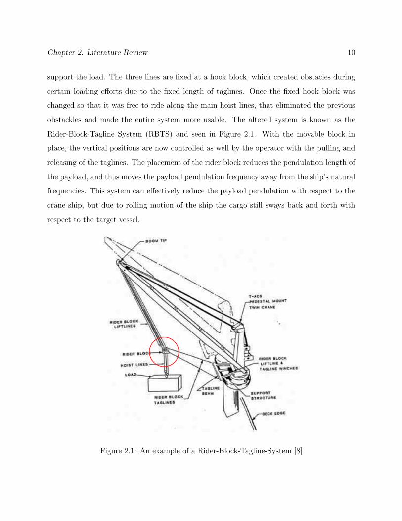
support the load. The three lines are fixed at a hook block, which created obstacles during
certain loading efforts due to the fixed length of taglines. Once the fixed hook block was
changed so that it was free to ride along the main hoist lines, that eliminated the previous
obstackles and made the entire system more usable. The altered system is known as the
Rider-Block-Tagline System (RBTS) and seen in Figure 2.1. With the movable block in
place, the vertical positions are now controlled as well by the operator with the pulling and
releasing of the taglines. The placement of the rider block reduces the pendulation length of
the payload, and thus moves the payload pendulation frequency away from the ship’s natural
frequencies. This system can effectively reduce the payload pendulation with respect to the
crane ship, but due to rolling motion of the ship the cargo still sways back and forth with
respect to the target vessel.
Figure 2.1: An example of a Rider-Block-Tagline-System [8]

Chapter 2. Literature Review 11
In order to overcome the deficiencies of the RBTS, a passive RBTS system was developed
by the Navy and was demonstrated onboard the T-ACS 5 vessel. In this system, an IMU
measures the vertical ship motion [9]. The controller takes in the information from the
vertical velocity and defines a horizontal motion, vertical motion of the rider block and rate
of change of the inhaul angle. This yields a movement of the liftline and taglines that can
compensate and keep the payload at a fixed inertial height. However, this system does not
compensate for the horizontal ship motion.
Then in 1999, Sandia National Labratories developed a Pendulation Control System (PCS)
that controls three-dimensional payload motion [10] and was also demonstrated onboard
the same T-ACS 5 vessel. The current system uses a position-based control that requires
the translational coordinates of the ship, the crane, and the payload swing angles. An
accurate and expensive ship navigation system, the POS/MV, is used to measure the 6
ship states. This GPS/IMU package also contains two GPS receivers to measure the current
position. The control system compensates the ship motion in order to prevent payload swing.
By assuming the payload swing angles are accurate the payload swing can be rejected.
This system also avoids operator commanded payload swing due to modifications to the
commanded crane signals from the joystick. This system showed promising performance
during sea trials.
2.2 Alternate Solutions
There are numerous other attempts at crane control using varying control methods and de-
sign. Wagner Associates, Inc. developed an anti-sway crane called Smartcrane [11] that uses
a combination of a “bang-bang” method–in which the acceleration of the pivot is corrected
to remove the sway to the load everytime the fulcrum is moved–and a method in which a
sensor determines amount of sway and a control algorithm adjusts the fulcrum. This system
cannot compensate for the motion of the crane platform as it is ideally situated on ground.

Chapter 2. Literature Review 12
There are others who use open-loop techniques in their control algothrim, such as Sakawa
et al. [12], in which they use an optimization technique to generate a torque profile to transfer
a load along a pre-defined path while minimizing the payload pendulation. This model was
simulated at a constant luff angle, and shows payload pendulation develop along the path
and increase as the slew angle increases. Takeuchi et al. [13] developed a strategy to achieve
a time-optimal slew-only motion, while reducing pendulation similar to those used on a
gantry crane. However, simulations have shown that this strategy suppresses out-of-plane
pendulation, but not in-plane pendulation.
Some of the closed-loop techniques came from Sakawa and Nakazumi [14] in which they
used an open-loop controller to track the trajectory of the boom, and a LQR optimized
state feedback controller controls the slew, luff, and hoist to eliminate residual pendulation
at the end of maneuver. Simulations were unsuccessful as there were high pendulation angles
during the maneuver. Nguyen et al. [15] proposed a feedback control strategy that uses two
independent controllers. One to control the boom’s luff angle and payload pendulation, and
another to control the hoisting. Tests show that transient pendulation was reduced, but there
were oscillations of the boom around the path, and steady-state errors occur in the boom
angle and cable length. Gustafsson [16] used a control strategy using independent in-plane
and out-of-plane, linear position feedback controllers based on partial linearization of the
spherical pendulum to reduce inertia-induced payload pendulum. Simulation results show
stable responses for operator commanded slewing rates away from the natural frequency of
the cable, with the payload having small pendulation angles. Chin et al. [17] proposed a
nonlinear feedback control to suppress the parametric instabilities in payload motion due to
base excitation. It introduced a harmonic change in the cable length at the same frequency
as the base excitation to suppress the instability and result in a smooth response. Abdel-
Rahman and Nayfeh [18] used the reeling and unreeling of the cable to avoid pendulation
motions in 3-D when base excitation approach natural frequency of the entire assembly. Such
a scheme changes the dynamics of the payload motion, and allows the primary controller

Chapter 2. Literature Review 13
to damp a planar motion instead of dampening a 3-D motion. Nayfeh et al. (2003) also
used a delayed-position feedback together with luff and slew angle actuation to control cargo
pendulation.
Various structurally different designs to stabilize the cargo swing are also readily available.
For example, Belsterling [20] suggests a multi-cable crane system that uses operator control
by comparing cargo location with the location of a beacon using a combination of inertial
sensor, distance sensor, camera, and light source. An idea by Lee [21] describes the use
of a transverse frame that bridges two ships. It includes articulate arms and spreader bar
mounted on the frame. Sensors would track the movement of the vessel, and automatically
responsive controllers would automatically adjust motion and position of the spreader bar
to follow the motion of the vessel. Holland et al. [22] came up with a robotic cable array
system where cables from three or more folding, telescoping masts located on each corner of
the vessel help to guide the cargo with the aid of various sensors and cameras. These ideas
have not caught on primarily due to their complexity and impracticality.
2.3 Summary
In this chapter we presented some of the research that happened at the start of the effort
to reduce pendulation swing for cargos during transports. Then we discussed literature
reviews on various methods of crane control to reduce pendulation swing on the cargo. These
methods include using different control algorithms including open-loop, closed-loop systems,
as well as those that use entirely different structural designs to overcome the problem. Next
chapter includes additional background information on the sensors that are used to help
operate the cranes and stabilize the payloads.

Chapter 3
Sensor Details
3.1 How IMUs Operate
Sensors are the tools one uses to determine the state of another object. In our case,
inertial sensors that feature gyroscopes and accelerometers provide information about po-
sition, velocity, acceleration, and angles with the aid of a computer. Generally, a group of
three accelerometers orthogonally mounted on a gyro-stabilized element forms the basis to
an Inertial Measurement Unit (or IMU).
The most basic form of an accelerometer measures a force based on deflection of a movable
mass that is constrained by two equal springs. That deflection is taken as a measure of the
acceleration. When the measurement includes a vertical component, the gravitational force
of Earth needs to be taken into account so that a distinction can be made between the actual
acceleration of the instrument relative to a point on the earth and the effect of gravity at a
stationary point. However, a couple of natural phenomenon can also affect the gravitational
readings. First, the centripetal acceleration that come from planet’s rotation is the greatest
(about 3 mg) at the equator and zero at the poles. Second, the gravitational values also
vary depending on the latitude because the Earth is not an exact sphere. Therefore, the
14

Chapter 3. Sensor Details 15
gravitational readings are susceptible to influences from additional tidal forces caused by the
moon [23]. In our simplified study, we assume the influences from the planet rotation, the
moon, and the bulge of the Earth, do not come into play.
3.2 Types of IMU Corruptions
As mentioned in the previous section, corruptions can creep into the data due to various
factors. The most common type of corruptions are the scale factor, bias, random drifts,
white noise, and several others. A brief explanation of each type of error is detailed in the
sections that follow.
3.2.1 Scale Factor
The scale factor is the ratio between a change in the output signal and the change in the
true input. Most sensors provide the output signal as directly proportional to the input
signal. However, if calibration is not perfect, the sensed motion will always be some percent
too small or too big. Therefore, the scale factor is usually a single number representing
the slope of the best-fit-line that results from applying a least squares method to the data
obtained by varying the input over a specific range. The scale factor can be seen in Figure 3.1
as the difference in the slope between the ideal and the actual data. It should be pointed out
that accelerometer scale factor only causes error when there is acceleration. Scale factors are
sometimes listed as a percentage. For example, a 1% scale factor in an environment where
there is a 2g acceleration can yield an uncertainty of 20mg. The more accurate sensors have
smaller scaling factors. However, different publications show scale factor in different ways,
such as using the inverse of the scale factor in units of deg/h/mA, deg/h/Hz, g/Hz.
The rate gyros have scale factor errors as well. The scale factor for rate gyros are im-
portant because the gyros must measure all the angular rates in order to help determine an

Chapter 3. Sensor Details 16
Figure 3.1: Example of a scale factor error
orientation. Scale factor may very well play a part in corrupting the sensor readings. In this
study, we are not focusing at the gyro errors because we are assuming the gyro readings are
perfect. The scale factor error is usually referred to in units of ppm, and deg/time.
3.2.2 Bias
The bias of a sensor is generally caused by miscalibrations, imperfections during manufac-
ture, the weather, and it appears even when there is no input. The bias is measured in units
of gravity g for an accelerometer, and a change in angle over time for a gyro. As with any
corruption, the lesser this value, the better the sensor. An example of the constant offset
can be seen in Figure 3.2. It is important to remove the offsets before further calculation
because sensor bias is the source for integration instabilities. Thus affecting the subsequent
velocity and position data that is mentioned in Chapter 4. In actuality, bias in IMUs are
not constant. As long as these biases do not vary significant amount over time during the
crane operation, it is reasonable to assume they can be filtered out by software since we do
not require the exact bias in our ship motion estimation.

Chapter 3. Sensor Details 17
Figure 3.2: Example of a bias
3.2.3 Random Drift
Within each day, natural conditions in the environment can change the scale factor and
bias by as much as 10 times compared to their in-run random drifts [23]. These natural
conditions include the temperature, amount of vibration, and magnetic fields at the time.
The aging of internal components (or in-run drifts) and other contamination can cause a
slow change over time. Noise may have peaks at different frequencies. In the case of gyros,
the ball bearing may produce noise depending on the ball size, number of balls, operating
speed, etc. This study does not include random drifts.
3.2.4 White Noise
White noise is an erroneous input signal which is random. The quality of a sensor is one
factor in determining how much white noise exists. As seen in the example in Figure 3.3,
they fluctuate about an ideal set of data. These noise levels usually have small effects on the
crane performance. The signals that have noise can be improved drastically with successive
integration steps as we shall see. For this study, no gaussian noise levels were considered
because the small noise levels do not introduce any significant corruptions in the integrated
states.

Chapter 3. Sensor Details 18
Figure 3.3: Example of white noise corruption
3.2.5 Other Errors
There are other sensor corruptions such as random walk, which is a long-term growth in
angle error. Sensors have a lower limit in which they cannot detect input changes below a
certain limit, or dead band. In cases of noisy sensors, a threshold defines the largest value of
minimum input (around zero) that produces an output of at least half expected value. The
resolution of a sensor can affect the accuracy readings for all the inputs as it is defined as the
largest value of the minimum input that produces an output proportional to the expected
value using the scale factor. Other sources of error exists, but they do not fall within the
scope of this project. It should be further noted that the concentration of this study is not
on the gyro errors as the gyro is assumed to be perfect for this part of project.
3.3 Types of IMU Sensors and Cost
IMU sensors can generally be split into three different grades based on their accuracy.
Naturally the cost is proportional to these accuracy levels. The three grades are 1) low
grade, 2) tactical or high grade, and 3) inertial or navigational grade. Generally, a low grade
IMU has a resolution of around 1 deg/sec for its gyro, and an accelerometer bias on the order
of g. An example of a low grade IMU would be the micromachined silicon accelerometer

Chapter 3. Sensor Details 19
(MSA). These devices are generally used in cars with a gyro resolution of 0.5 deg/sec [24],
and usually costs less than $100. Their size is usually small, making them more portable
and easier to implement.
The next grade of IMU is the tactical or high grade that has a gyro resolution on the
order of 10−2 deg/sec and an accelerometer bias on the order of milli-g. This class of IMUs
generally cost in the thousands of dollar range and are widely used in industry.
The last grade of IMU is the inertial or navigational grade. They are the most accurate
IMU sensors having a gyro resolution on the order of 10−3 deg/sec and an accelerometer
bias on the order of micro-g. The cost of one of these units is in the tens to hundreds of
thousands of dollars range. Table 3.1 [26] lists some of the different IMUs out on the market,
along with their errors and estimated price range. It should be noted that the POS/MV 320
sensor shown in Figure 3.4 is the current GPS/IMU sensor package in use on the PCS. It is
also extremely accurate, and because it is used on the high seas, it is also considered part of
the marine grade of IMUs. Some of the error values from these sensors is used later in the
simulation to see whether the application of those sensors into the control algorithms will
yield useful results.
Figure 3.4: Existing GPS/IMU system, POS/MV 320 [25]

Chapter 3. Sensor Details 20
Table 3.1: Listing of IMU, errors and estimated cost.
Grade Navigation Tactical Low Grade
IMU Honeywell HG9900 Litton LN200 Crossbow IMU 400CA
Accelerometer Quartz Silicon Silicon
Bias <25µg 200µg - 1mg ±30mg
Scale Factor (ppm) <100 300 <10000
Noise - 50µg/√Hz 0.15 m/s/
√Hz
Gyro Ring Laser Fiber Optic MEMS
Bias (◦/h) <0.003 1-10 3600
Scale Factor (ppm) <5 100 <10000
Noise (◦/h/√Hz) <0.002 0.04-0.1 <0.85
Cost >$100,000 $20,000 $1,000-$10,000
3.4 Summary
In this chapter, the basic operation of an IMU was mentioned, as well as different types
of corruptions that usually occurs. Also described were various types of sensors out on
the market, and their approximate cost. Next chapter includes concepts that govern the
controllers which uses various results from sensors.

Chapter 4
Relevant Concepts
Before detailing the simplified one-dimensional cart pendulum simulation, it is important
to discuss some items used in the new rate-based control simulations. These include the
description and the selection of the frame of reference, some crane dynamics detailing the
ship-crane system, and the filtering process. The filtering process includes methods used
to conduct digital filtering, the choice of filters, as well as the expected frequency response
from our choice of filters. In order to demonstrate the behaviors of the filter, a simple one-
dimensional cart pendulum simulation showing the position-based control, similar to the
PCS that is currently onboard the Flickertail State, is used.
4.1 Slow Drifting Frame
Just like the existing position-based control solution, the rate-based control also relies on
a frame of reference that is not locked into an absolute inertial frame I. Meaning, we are
not looking at the ship’s position with respect to the Earth. If that were the case, then the
slow ship drifts caused by wind and sea conditions over time will fool the control and allow
the payload to move further away from the ship as time progresses. Instead, the main focus
21

Chapter 4. Relevant Concepts 22
falls on the drifting frame, I ′, from which the ship is allowed to drift slowly about a point as
seen in Figure 4.1. Selecting the anchor point of the crane ship as the reference point makes
sense because as the cargo vessels dock with the crane ship during transport operation, it
can be assumed that both ships move as a single entity. Therefore, as slow drifts occur, the
I ′ frame drifts along with the loading ship along with our crane ship.
Figure 4.1: Example of the slow drifting reference frame I ′
The frame I ′ is naturally aligned with the surge, sway, and heave axes of the ship, which
helps isolate some of the ship’s motions that occur. One of these motions is the short period
motion that is generally caused by the ship roll motion. Short period motion is the dominant
ship motion as its frequencies fall between 0.06 and 0.10 Hz. This range of frequencies also
falls within the range of the natural payload pendulation frequencies. So it is vital for the
control to compensate for this type of ship motion. Another type of motion is a long period
motion. However, the long period motion will not cause as large a payload swing as the

Chapter 4. Relevant Concepts 23
short period motion, and is therefore not considered a dominant motion. Slow drift about
the anchor point is an example of the long period motion. If the PCS were to account for the
slow drift over time, the control will react continuously without end as the control believes
the error is continually increasing.
4.2 Crane Kinematics
Now that the new inertial frame I ′ has been established, there are a couple more local
reference frames that need to be addressed as they play an important part in the dynamics
of the crane-ship system and the control solutions.
Each individual crane has a crane reference frame C with components {c1, c2, c3}. The c1
axis points straight ahead towards the bow of the ship. However, the axis does not have to
lie exactly on the centerline of the ship because the crane is not located on the centerline of
the ship. As shown in Figure 4.2, the c1 axis is aligned where the slew angle α is zero degree.
Using the normal right-hand rule notation, the c2 axis points toward the port (left) side of
the ship at a slew angle of +90◦. That makes the c3 axis point vertically and matches the
slew rotation axis of the crane. Figure 4.2 shows the top view that contains the slew angle,
as well as the c1 and c2 axes.
Figure 4.2: Top view showing crane frame and slew angle, α

Chapter 4. Relevant Concepts 24
The side view diagram of Figure 4.3 shows the slew axis c3 in relation to c1 which points
toward the bow of the ship. Note that the hinge of the boom does not lie on the slew
axis, and the distance between them is specified by ad. This offset is a factor during the
calculation of the dynamics. The boom length is indicated by the variable Lb, and the hoist
length is Lh. The β parameter indicates the crane luffing angle. Using trigonometry and
Figure 4.3: Side view showing crane frame and luff angle, β
the luff angle β, the boom tip position vectors with respect to the crane frame are expressed
using C frame components as:
Crb/C =
C(Lb cos β − ad) cosα
(Lb cos β − ad) sinα
Lb sin β
= ( )c1 + ( )c2 + ( )c3 (4.1)
where Crb/C is the vector from the crane frame origin to the boom tip in terms of the crane
frame C and its components c1, c2, c3.
In order to see the big picture of the entire ship/crane system, two other reference frames
need to be addressed. They are the inertial frame and the ship’s sensor frame–designated
by I and S, respectively. Both of these reference frames are seen in Figure 4.4. The inertial
frame used here is the same slow drifting frame I ′ described earlier. The ship’s sensor frame,

Chapter 4. Relevant Concepts 25
S with components {s1, s2, s3} is located on a fixed point onboard the ship. The S frame
does not need to be perfectly aligned to the vertical, or to the bow of the ship. The position
vectors and frame orientation at the crane frame relative to the ship frame can be attained
with proper measurements and calibrations.
Figure 4.4: Inertial, Ship Sensor, and Crane Coordinate Frames
Figure 4.4 illustrates all vectors that lead to the inertial final position of the payload given
by
rp/I = rS/I + rC/S + rb/C + rp/b (4.2)
The Crb/C term from Equation (4.1) is just one of the terms that makes up Equation (4.2).
Also, the swing position vector of the payload relative to the boom tip expressed using the

Chapter 4. Relevant Concepts 26
I frame is
Irp/b =
I0
0
−Lh
(4.3)
Note that the Irp/b term can also be represented as LhI g if there is zero swing, and only the
gravitational vector [0;0;-1] exists.
In their current state, the vectors in Equation (4.2) are all expressed respect to different
coordinate frames. The choice was made to use the I frame so that the inertial component
i3 is aligned to the direction of the gravity. In order to continue down this path, the ship
sensor frame S and the crane frame C components will require 3× 3 rotation matrices to get
them all into a common reference frame. As an example, the rotation matrix [IS] can map
the vector with S components into the I frame using the ship roll, pitch, and yaw angles
(φ, θ, ψ). Similarly, the [SC] rotation matrix can map components from the crane frame into
the ship’s sensor frame. After these two rotation matrices are known, the rotation matrix
[IC] can be found using the product of the two known rotational matrices
[IC] = [IS] [SC] (4.4)
It should also be noted here that in this particular case, the [SC] matrix is constant because
once the sensor is installed onboard, its distance and orientation relative to the crane frame
do not change. Now if we rewrite Equation (4.2) using the proper frame coordinates, it
appears as
I rp/I = IrS/I + [IS] SrC/S + [IC] Crb/C + Irp/b (4.5)
Equation (4.5) is key to conducting inverse kinematics calculations for both the current GPS
position based control solution, and the new rate-based control solutions that can use both
position and velocity. More specifically, some of the terms in Eq. (4.5) include the crane
states that stabilizes the payload such as the slew angle α, luff angle β, and the hoist length
Lh. By knowing these three main states, the controller can input a rate command so that the

Chapter 4. Relevant Concepts 27
crane will move a set amount to reach the specified states and thereby stabilize the payload.
More detail on the inverse kinematics of each type of controls is provided in Chapter 5.
4.3 Digital Filtering of Ship Motion Sensing
4.3.1 Advantages of Digital Filters
The use of digital filtering techniques is prevelant in modern industrial systems because
of the small sampling instants produced by today’s digital computer readouts. Usually,
the time interval between two sampling instants is so short that data between the instants
can be approximated by interpolation [27]. Digital filters are also easily programmable on
computers, therefore they can be changed without affecting any hardware. Working in a
virtual environment means that we do not have to deal with circuits, which leads to a
reduction of drifts, and makes the filter not temperature dependent. The digital filter also
handles low frequency signals accurately [28].
4.3.2 Application
In our case, the discretization process is used to approximate the readouts from the ac-
celerometer. The method in which we analyze the discrete-time system is with the Z-
transformation. The role of the Z-transformation in discrete-time systems is similar to that
of the Laplace transformation in linear, time-invariant, continuous-time systems. Such a
similarity between the two methods makes it possible for the formulas that generated our
digital filter algorithms to start off in Laplace space as X(s) and Y (s)–representing digital
signals x(t) and y(t), respectively. Then the input/output transfer function H(s) can be
expressed as the ratio of the output Y over the input X as
Y (s)
X(s)= H(s) (4.6)

Chapter 4. Relevant Concepts 28
A transfer function for the filter can be introduced as F (s), which takes the place of the
current transfer function H(s) in Eq. (4.6). With the new filter transfer function, one can
include any desired characteristics needed to be implemented into the filter. Some examples
include combining multiple types of filters, or a specific type of filter with a differentiation
term (by multiply by a s term) so that the transfer function serves both as a differentiator
and a signal filter. Including a 1s
term instead of the s term results in integration instead of
differentiation.
In order to map from the Laplace domain from Eq. (4.6) to the Z-domain, a trapezoidal
rule shown in Eq. (4.7) is applied because it is more versatile when dealing with differences
between the frequency of the sample and the critical filter frequency.
s =
(2
h
)1− z−1
1 + z−1(4.7)
The resulting s = f(z−1) function is substituted into Eq. (4.6) and results in the recursive
relationship
b0y +N∑
i=1
biyz−i = a0x+
N∑i=1
aixz−i (4.8)
With k as the time step, and the rule that
yz−1 = yk−ixz−1 = xk−i (4.9)
we get the filtered step at time step k with the following formula
yk =1
b0
[a0xk +
N∑i=1
(aixk−i − biyk−i)
](4.10)
The N represents the highest order in the transfer function H(s). The recursive formula in
Eq. (4.10) can be used for any combination of filters depending on its ai and bi values.
4.3.3 Filter Types
There are numerous digital filters and each serves its own purpose. Some of these filters
include lowpass, highpass, notch, bandpass filter, and all pass filters. There are filter types

Chapter 4. Relevant Concepts 29
that resemble a combination of multiple filter types, along with possible integration, differ-
entiation, and higher order version of these various filters. Each type of filter has its benefits
and drawbacks. For example, a lowpass filter can allow for low frequency signals to pass,
but it produces a phase lag. A highpass filter can allow high frequency signals to pass, yet
it results in a phase lead. An allpass filter changes the signal phase but not its amplitude.
A notch filter allows the lower and higher frequencies to pass, forming a valley in the middle
of its magnitude bode plot. The bandpass filter has characteristics that is the opposite of
the notch filter because it allows the signals within a certain range around a predetermined
center frequency to pass, and filters out rest of the signals. The bandpass filter is in essence
a compromise between a lowpass and highpass filter. It acts as a highpass filter for low
frequencies and lowpass filter for high frequencies.
4.3.4 Filter Selection and Algorithm
The bandpass filter is chosen to filter out certain ship motion in the current PCS system
because it is a combination of a highpass and lowpass filter. Just like the notch filter, the
bandpass filter also employs a bandwidth, BW , that specifies a symmetrical range around a
center frequency, ωc. Any signal with frequencies above or below that range is filtered out.
As with all filters, a 1st-order filter can reject a constant signal x. A 2nd-order filter can
reject a linearly growing signal over time, and so on. However, only two orders are needed
for the existing GPS-based PCS because as the order of the filter increases, so follows the
sensitivity of the center frequency. The higher order filter will cause the entire filter to be
less robust as a result. Thus, the use of a 1st or 2nd-order bandpass filters are sufficient to
cancel out the linearly growing signal terms that will come out of our integration steps.
The 1st-order transfer function of bandpass filter is seen by Eq. (4.11).
Y (s)
X(s)=
sBW
s2 +BWs+ ω2c
(4.11)

Chapter 4. Relevant Concepts 30
The 2nd-order transfer function is merely the square of the 1st-order with an extra dimen-
sionless damping term ξ, as seen in Eq. (4.12).
Y (s)
X(s)=
BW 2s2
(s2 + ω2c )
2 + 2BWsξ(s2 + ω2c ) +BW 2s2
(4.12)
After performing the Z-transform in Eq. (4.7), both bandpass digital filter’s 1st and 2nd-
order recursive algorithm are as follows:
yk =1
4 + 2hBW + h2ω2c
[yk−1(8− 2h2ω2c )
+ yk−2(−4 + 2hBW − h2ω2c )
+ 2hBW (xk − xk−2)]
(4.13)
yk =1
4h2BW 2 + (4 + h2ω2c )
2 + 4hBW (4 + h2ω2c )ξ
[
yk−1(4(4− h2ω2c )(4 + h2ω2
c + 2hBWξ))
+ yk−2(2(−48 + 4h2BW 2 + 8h2ω2c − 3h4ω4
c ))
+ yk−3(4(4− h2ω2c )(4 + h2ω2
c − 2hBWξ))
+ yk−4(−4h2BW 2 − (4 + h2ω2c )
2 + 4hBW (4 + h2ω2c )ξ)
+ 4h2BW 2(xk − 2xk−2 + xk−4)]
(4.14)
The units for BW is in Hz, center frequency ωc is in rad/s, and digital sampling period h in
seconds. As mentioned before, the xk, yk terms represent the current ship state measurement
and the filtered ship state at current time step k, respectively. Thus, the xk−1 and yk−1
represent their previous time step measurement.
4.3.5 Filter Behaviors on POS/MV Based Control
We apply the recursive algorithm for the bandpass filter in Eq. (4.14) to the POS/MV
based control, which is the current GPS/IMU system that is onboard the crane ship. The
outcome allows us to see the effects of the filters in the context of the control system. As
seen from the diagram in Figure 4.5, the input xtrue is a prescribed true position of the ship.

Chapter 4. Relevant Concepts 31
Figure 4.5: Filtering Process of POS/MV Based Control
The true position is then corrupted with a sensor drift that was applied using real error data
for a good, medium, and bad days. A MATLAB code was written by my colleague Chris
Romanelli, that represents these data as corrupted signals over a user defined time duration
and time step. The different outputs of these drift conditions can be observed in Figure 4.6.
The signal that comes after the drift corruption is a sensed position, xsensed. Using the
2nd-order bandpass filter as seen in Equation (4.14), we were able to get rid of the drift and
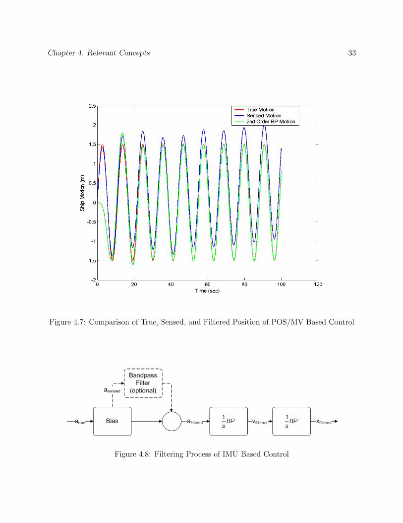
stabilize the payload. A plot of the true, sensed, and filtered position is seen in Figure 4.7.
In the plot, the red line indicates the prescribed true position. It deviates from the blue
line, which shows the drift corruption that was added. The green line represents the filtered
position, which was not in sync with the true position (red) at the start. But as time goes
on, one can see the filter doing what it should be doing as the filtered and the true positions
match very closely with each other. Thus, the filter meets its goal of eliminating drifts.
4.3.6 Filter Behaviors on IMU-Based Control
We see the filtering technique work for a model of the existing pendulation control, now it
is time to try it on the newly proposed IMU-based controls. The IMU-based controls include
both rate-based control solution that use both position and velocity. As seen in Figure 4.8,
the process starts off with a prescribed true acceleration reading from the accelerometer.
That signal is then corrupted with a constant accelerometer bias and scaling factor that
results in a sensed accelerometer reading, asensed. An optional 1st-order bandpass filter can
be placed here to eliminate the constant offset caused by the bias. The resulting signal
will be a filtered acceleration reading, which is then put through a recursive algorithm that

Chapter 4. Relevant Concepts 32
Figure 4.6: Error signals on a)Calm Day, b)Medium Day, c)Rough Day
Chapter 4. Relevant Concepts 33
Figure 4.7: Comparison of True, Sensed, and Filtered Position of POS/MV Based Control
Figure 4.8: Filtering Process of IMU Based Control

Chapter 4. Relevant Concepts 34
integrates and has a 1st-order bandpass filter component. The filtered velocity, vfiltered is
the outcome. The IMU based control that uses only velocity will pass this result onto the
controls. Even though only the velocity is used, a position reading still needs to be obtained.
The reason for this will be explained later in the controls section in Chapter 5. The same step
that got us velocity from acceleration reading will get us the position readings from velocity
in terms of putting the signal through an integrator and a 1st-order bandpass combination.
This results in a filtered position, xfiltered. Trial runs that support the use of this additional
1st-order filter can be seen in Chapter 6.
4.4 Summary
In this chapter, we identified several local and inertial coordinate frames and their rela-
tionship with each other through a series of vectors. The basics of digial filtering and ship
motion sensing was also discussed as it deals with smoothing out corruptions that come from
the sensor data. Current PCS data were used to show the effectiveness of digital filtering.
Next chapter, we apply all that we have seen up to now and use them in the new rate-based
control solutions.

Chapter 5
Differences Between Control Solutions
5.1 3D Inverse Kinematics
The method of inverse kinematics is useful in cases when a final condition is known, but
the parameters that lead up to the final condition are unknown. This is in contrast to
normal kinematics in which a certain number of parameters are given or can be solved for
that leads to a final solution. Inverse kinematics applies in our crane control scenario because
the location of the payload is known due to the need to keep it stable. However, the boom
orientations (slew & luff angles, and the hoist length) are the unknowns. Once these three
crane state parameters are known, they are passed into the control system. In the current
POS/MV based system, the three parameters are just the two angles, slew & luff, and the
hoist length. In the IMU based control solution that uses velocity, the rate of the slew and
luff angle, and the rate that the hoist length moves are the control inputs. The inverse
kinematics of the IMU based control that uses position relies on the same parameters as the
POS/MV based control, the only difference lies in the method used to sense ship position
states.
35

Chapter 5. Differences Between Control Solutions 36
5.1.1 3D Inverse Kinematics of Position Based Control
For the control solution that is position based, the main goal is to obtain the crane position
and then numerically differentiate its crane states to be used by the crane’s servo system.
From Equation (4.5) and Figure 4.4, we see that the vector rp/I is the desired payload position
in the inertial frame. This may be called a nominal position as well, where the payload swing
is nonexistent. From this configuration, the ideal crane states can be calculated. We start
with showing the unit gravity vector g in terms of the crane and the inertial frame as
g = −i3 =
Cg1
g2
g3
= [CI]
I0
0
−1
(5.1)
With vector g, the payload position vector with respect to the boom tip can be written as
Crp/b = LhCg (5.2)
Using the above equation, Equation (4.5) can be rewritten in the crane frame C as
[CI](I rp/I − IrS/I − [IS] SrC/S
)= Crb/C + Lh
Cg (5.3)
and the right side of the equation involves the crane states α, β, and Lh. They are represented
in the crane frame as
Crb/C + LhCg =
C(Lb cos β − a) cosα+ Lhg1
(Lb cos β − a) sinα+ Lhg2
Lb sin β + Lhg3
(5.4)
The result of Equation (5.4) produces the three necessary crane states, but its nonlinear
equation needs a quintic polynomial function to solve for (α, β, Lh).
In the inertial frame, we do not need to know the ship motion respect to the true inertial
frame, only the slow drifting frame. Therefore, we see a nominal payload position as having

Chapter 5. Differences Between Control Solutions 37
zero translation with respect to the drifting frame. So, if a slew or luff maneuver is performed,
then the nominal angles for both slew and luff parameters are increased. It is also assumed
that there is no swing of the payload. Similar to Eq. (4.1), using the nominal slew α and
luff β, the nominal boom tip position relative to the crane frame C is
Crb/C =
C(Lb cos β − a
)cos α(
Lb cos β − a)
sin α
Lb sin β
(5.5)
Not forgetting the nominal hoist length Lh, the payload’s position vector relative to the
boom tip is
I rp/b =
I0
0
−Lh
(5.6)
With the Crb/C and I rp/b terms, the nominal inertial payload position can be computed with
I rp/I =(S rC/S + [SC] Crb/C
)+ Iδr + I rp/b (5.7)
The boom tip damping correction is the δr term included to damp out swings. A pre-selected
gain value is attached to this term which moves the boom tip in the opposite direction as the
sensed swing, thus dampens the pendulation swing. The gain value matches the value on
the real PCS and is unchanged here. This is simply a small position vector that approaches
zero if the swing angle goes to zero. When compared to the overall vector equation (4.5), one
difference is the missing rotation matrix, [IS]. That matrix essentially cancels out because
we assume the nominal ship frame to have the same attitude as the inertial frame, so there is
no orientation difference, resulting in [IS] being an identity matrix. In the end, the nominal
payload position rp/I can be computed if we know the nominal crane states α, β, and Lh,
as well as the boom tip’s Cartesian damping correction δr.

Chapter 5. Differences Between Control Solutions 38
5.1.2 3D Inverse Kinematics of Velocity Based Control w/ IMU
The IMU-based control senses the ship motion with accelerometer and rate gyro data, as
well as the true roll and pitch angles. The inverse kinematics of the velocity based control
directly computes the crane rates that is used to control the crane to compensate for the
measured ship motion.
In section 4.2, Equation (4.2) shows the payload position vector. Then, the payload
velocity becomes the time derivative of the position.
rp/I = rS/I + rC/S + rb/C + rp/b (5.8)
However, when taking the time derivative of the position vector, one must take into account
that the base vector directions of the chosen coordinate system may be time varying also.
Thus, a transport theorem [31] is used that allows one to take the derivative of a vector
with respect to one coordinate system, even though the vector itself has its components in
another system. For example,Sdxdt
stands for the time derivative of x seen by the S frame.
In our case, the vector rC/S is expressed in the S frame, and the rb/C in the C frame, the
transport theorem has to be used. The resulting payload velocity in inertial frame is
rp/I = rS/I +Sd
dt
(rC/S
)+ ωS/I × rC/S +
Cd
dt
(rb/C
)+ ωS/I × rb/C + rp/b (5.9)
It should be noted that the the vector, rC/S , from the sensor to the crane frame is a constant
as seen by the ship frame, so its derivative is zero. Also, the ωS/I term has three components
that are the rate measurements from the gyro sensor. The crane boom tip position term rb/C
is seen in Eq. (4.1). Here, we need to take its derivative as seen by the C frame, which is
Cd
dt
(Crb/C)
=
C−(Lb cos β − a) sinαα− Lb sin β cosαβ
(Lb cos β − a) cosαα− Lb sin β sinαβ
Lb cos ββ
(5.10)

Chapter 5. Differences Between Control Solutions 39
where the position vector of the payload rp/b relative to the boom tip in the inertial frame
is seen in Equation (5.6), its derivative is simply
rp/b =
I0
0
−Lh
= Lhg (5.11)
The previously defined gravity vector is in terms of the inertial frame. In order to convert
this vector to the crane frame, rotation matrix [IC] is needed so that
Cg = [IC]T
0
0
−1
= [IC]T I g =
Cg1
g2
g3
(5.12)
Now if we substitute Eq. (5.12) and Eq. (5.8), we get
N rp/I − N rS/I − [IS](SωS/I × SrC/S
SωS/I × [SC] Crb/C)
= [IC]
( Cd
dt
(Crb/C)
+ [CN ]N rp/b
)(5.13)
In the above equation, the vectors are in several different frames I, S, and C. The rotation
matrices [SC] and [IS] are the same, and the matrix [IC] maps components from the crane
frame to the inertial frame. Terms on the left hand side include inertial payload velocity,
inertial ship motion velocity, attitude matrix of the ship, ship’s rotation rate, and the boom
tip position vector. The right hand side includes the rate of the ship crane states that we
need. The right hand side of the equation is equivalent to the following equation
Cd
dt
(Crb/C)
+ LhCg (5.14)
Transforming eq. (5.14) into its matrix form results in,
Crb/C =
−(Lb − a) cos β sinα −Lb sin β cosα g1
(Lb − a) cos β cosα −Lb sin β sinα g2
0 Lb cos β g3
α
β
Lh
(5.15)
Once we have sensor measurements and a nominal inertial payload velocity, we can calculate
the left hand side of the Equation (5.13). Then, we can take the inverse of the 3 × 3 matrix
Chapter 5. Differences Between Control Solutions 40
and multiply that by the known left hand side values to get us the necessary α, β, Lh values
needed for the control.
The inverse kinematics of the velocity-based control requires a nominal inertial payload
motion. Similar to the position-based inverse kinematic solution, we can use the nominal
crane concept to get a nominal inertial payload velocity vector ˙rp/I . The nominal inertial
payload position can be seen in Eq. (5.7). One needs to keep in mind that the term rC/S is
constant. Therefore its derivative is zero. If we take the derivative of rp/I , then the nominal
inertial payload velocity vector is
˙rp/I =(˙rb/C
)+ δr + ˙rp/b (5.16)
The rate of the damping correction term δr is computed by numerically differentiating the
δr term from the position-based control, and the ˙rb/C term from Eq. (5.10). In the end, the
nominal payload velocity ˙rp/I can be computed if we know the nominal crane rates ˙α, ˙β,
and ˙Lh, as well as the rate of boom tip’s Cartesian damping correction δr.
5.2 Simplifying from 3D to 1D
It is common perception that any three-dimensional system is more complicated than a
one-dimensional system. The crane system is no different. The crane dynamics alone adds to
the complexity of any simulation, which does not even include all of the various mechanical
devices onboard the crane that needed to be simulated. In real life, mechanical parts are
never absolutely perfect. In our boom crane, sources of imperfection can stem anywhere from
the crane’s hydraulic systems such as winches, servos, various measurement sensors, not to
mention the unpredictability from the ocean itself. The full three-dimensional simulation
that is used to model the existing PCS has to be as detailed as possible. Numerous biases
and noises are included within the full simulation to ensure the maximum amount of realism.
On top of that, the full three dimensional equation of motion is quite extensive, as can be
Chapter 5. Differences Between Control Solutions 41
seen in [29]. Whereas if one were to make use of a less complicated system of equations to
model the same problem, it will be easier to do control designs.
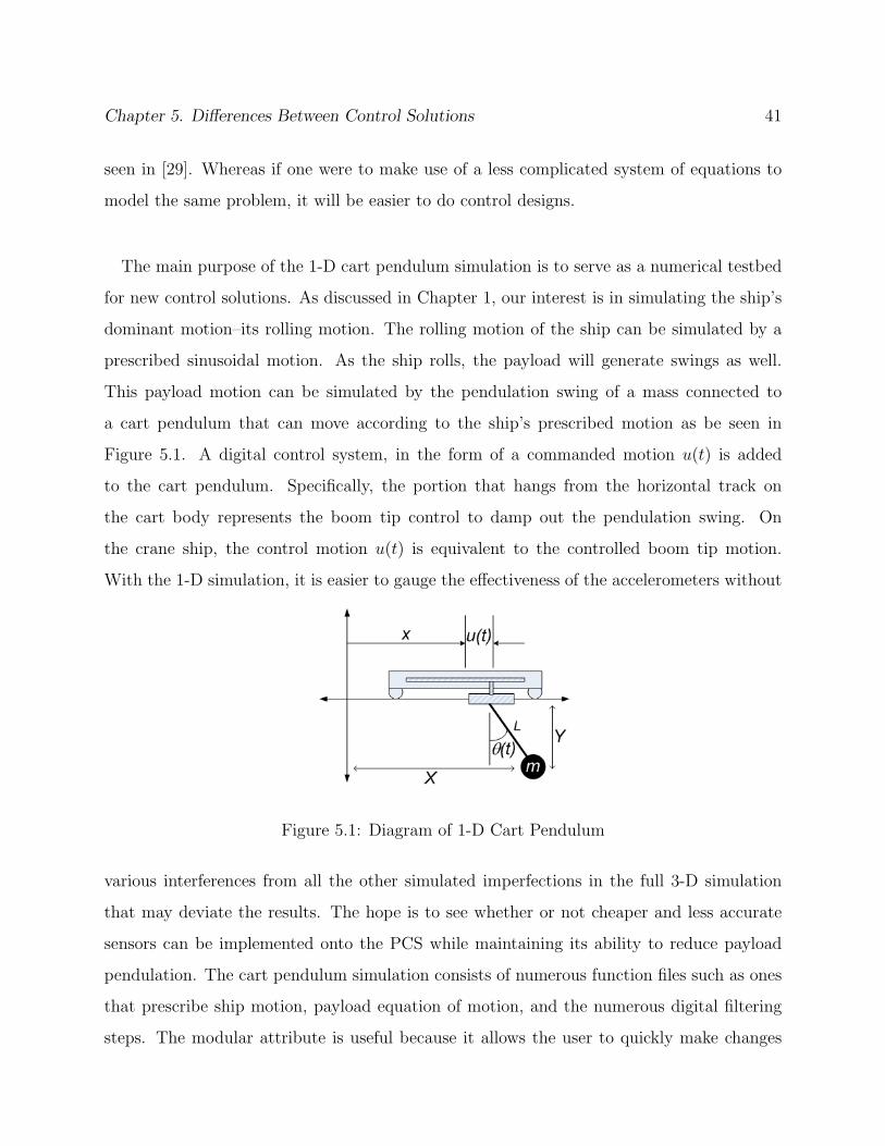
The main purpose of the 1-D cart pendulum simulation is to serve as a numerical testbed
for new control solutions. As discussed in Chapter 1, our interest is in simulating the ship’s
dominant motion–its rolling motion. The rolling motion of the ship can be simulated by a
prescribed sinusoidal motion. As the ship rolls, the payload will generate swings as well.
This payload motion can be simulated by the pendulation swing of a mass connected to
a cart pendulum that can move according to the ship’s prescribed motion as be seen in
Figure 5.1. A digital control system, in the form of a commanded motion u(t) is added
to the cart pendulum. Specifically, the portion that hangs from the horizontal track on
the cart body represents the boom tip control to damp out the pendulation swing. On
the crane ship, the control motion u(t) is equivalent to the controlled boom tip motion.
With the 1-D simulation, it is easier to gauge the effectiveness of the accelerometers without
Figure 5.1: Diagram of 1-D Cart Pendulum
various interferences from all the other simulated imperfections in the full 3-D simulation
that may deviate the results. The hope is to see whether or not cheaper and less accurate
sensors can be implemented onto the PCS while maintaining its ability to reduce payload
pendulation. The cart pendulum simulation consists of numerous function files such as ones
that prescribe ship motion, payload equation of motion, and the numerous digital filtering
steps. The modular attribute is useful because it allows the user to quickly make changes
Chapter 5. Differences Between Control Solutions 42
as they focus on a specific part of the simulation. The modular nature of the program also
creates ease for the user as they do not need to go through all the lines of codes in a long
sequential file. If the test case shows promise in the simpler cart pendulum simulation, then
it can be modified to be used on the full-scale simulation for more realistic results.
The rest of this chapter includes the derivation of the equations of motion for the cart
pendulum system. The equations of motion are incorporated into both the rate-based po-
sition and velocity control simulations. The differences between the two type of rate-based
control solutions are explained as well.
5.3 Equations of Motion
5.3.1 Derivation Using Lagrange’s Equation
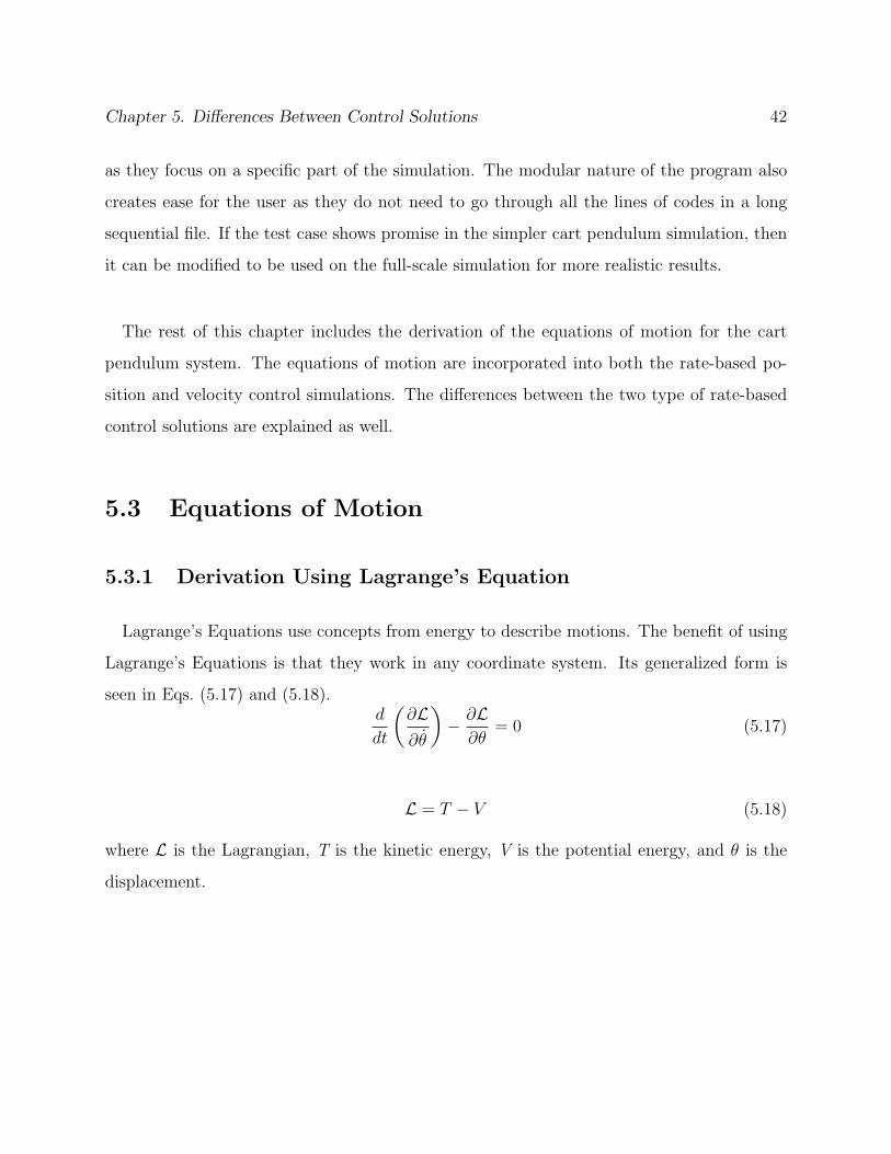
Lagrange’s Equations use concepts from energy to describe motions. The benefit of using
Lagrange’s Equations is that they work in any coordinate system. Its generalized form is
seen in Eqs. (5.17) and (5.18).d
dt
(∂L∂θ
)− ∂L∂θ
= 0 (5.17)
L = T − V (5.18)
where L is the Lagrangian, T is the kinetic energy, V is the potential energy, and θ is the
displacement.

Chapter 5. Differences Between Control Solutions 43
5.3.2 Applying Lagrange’s Equation to the 1-D Cart Pendulum
The Cartesian coordinate system is used for this cart pendulum simulation. The resulting
kinetic energy T, and the potential energy V are
T =1
2mV 2 =
m
2
(X2 + Y 2
)(5.19)
V = −mgL cos θ (5.20)
It should be noted that the V in Eq. (5.19) is the velocity term, which was then broken
down into the derivatives of its x and y position components centered around the origin. As
illustrated in Figure 5.1, the position in the horizontal and vertical direction are as follows
X = x(t) + u(t) + L sin θ(t) (5.21)
Y = −L cos θ(t) (5.22)
The x(t) is the x-position of the cart, that represents the ship rolling motion. The u(t) is
the commanded position control that reacts to the change in the x-position, and is located
in the boom tip. The L is the length of the hoist cable, and θ(t) is the swing angle at a time
t. Take their derivatives with respect to time, and the resulting velocity components become
X = x+ u+ L cos θ · θ (5.23)
Y = L sin θ · θ (5.24)
Use the results from Eq. (5.23) and (5.24) and substitute into Eq. (5.19). With all of the
kinetic and potential energy terms present, Eq. (5.18) can be completed. The last step is
to take the partial derivatives and the normal derivatives as seen in Eq. (5.17). Thus, the
non-linear pendulation equation becomes:
θ +
(x+ u
L
)cos θ +
g
Lsin θ = 0 (5.25)
In order to make the equation of motion in Eq. (5.25) work with the simulations, it has
to be converted from a single 2nd-degree non-linear differential equation into a system of

Chapter 5. Differences Between Control Solutions 44
two-1st degree equations. Within the programs, variables X1 = θ and X2 = θ represent the
swing angle, θ, and the swing angle rate, θ, respectively. In doing so, the system of equations
that is used throughout the cart pendulum simulations is
θ =d
dt(θ) (5.26)
θ = −(x+ u
L
)cos θ +
g
Lsin θ (5.27)
Equations (5.26) and (5.27) are the equations of motion for the simplified 1D cart pendulum
system.
5.3.3 Solving the Equations of Motion
In order to solve the system of differential equations and let it be applicable to the dis-
cretization process, numerical analysis is applied. More specifically, the Fourth Order Runge-
Kutta method is selected to solve the equations. Other methods, such as the Taylor method,
have the desirable property of high-order local truncation error, but it requires the compu-
tation of derivatives of the function. Taylor method tends to result in a complicated and
time-consuming process, which is why it is not used. The benefit of the Runge-Kutta method
is that it has high-order local truncation error of the Taylor methods, while eliminating the
need to compute and evaluate derivatives by using an iterative process as seen below. The
differential form of Runge-Kutta method of order four is the following [30].
w0 = α (5.28)
k1 = hf(ti, wi) (5.29)
k2 = hf
(ti +
h
2, wi +
1
2k1
)(5.30)
k3 = hf
(ti +
h
2, wi +
1
2k2
)(5.31)
k4 = hf(ti+1, wi + k3) (5.32)
wi+1 = wi +1
6(k1 + 2k2 + 2k3 + k4) (5.33)

Chapter 5. Differences Between Control Solutions 45
for each i = 0, 1, ..., N − 1. The variable α is an initial value, h is the time step, t is the
specific time, and w keeps track of the answer to each iterative process. The Runge-Kutta
method is used in all of the cart pendulum simulations related to this project.
5.4 Simplified 1D Control Using Position Based In-
verse Kinematics
The flowchart shown in Figure 5.2 is the general flowchart of the position-based control
solution that uses the IMU for the 1-D cart pendulum simulation. Please note that this is the
Figure 5.2: Flowchart of the Rate-Based Position Control
exact same control system as the current PCS and nothing is changed or added. The input
signal comes from the accelerometer data to simulate the ideal ship motion. In this case, it
is the ship’s rolling motion that is being simulated as mentioned in a previous section. This
acceleration is the true acceleration and is represented by the atrue symbol in the flowchart.
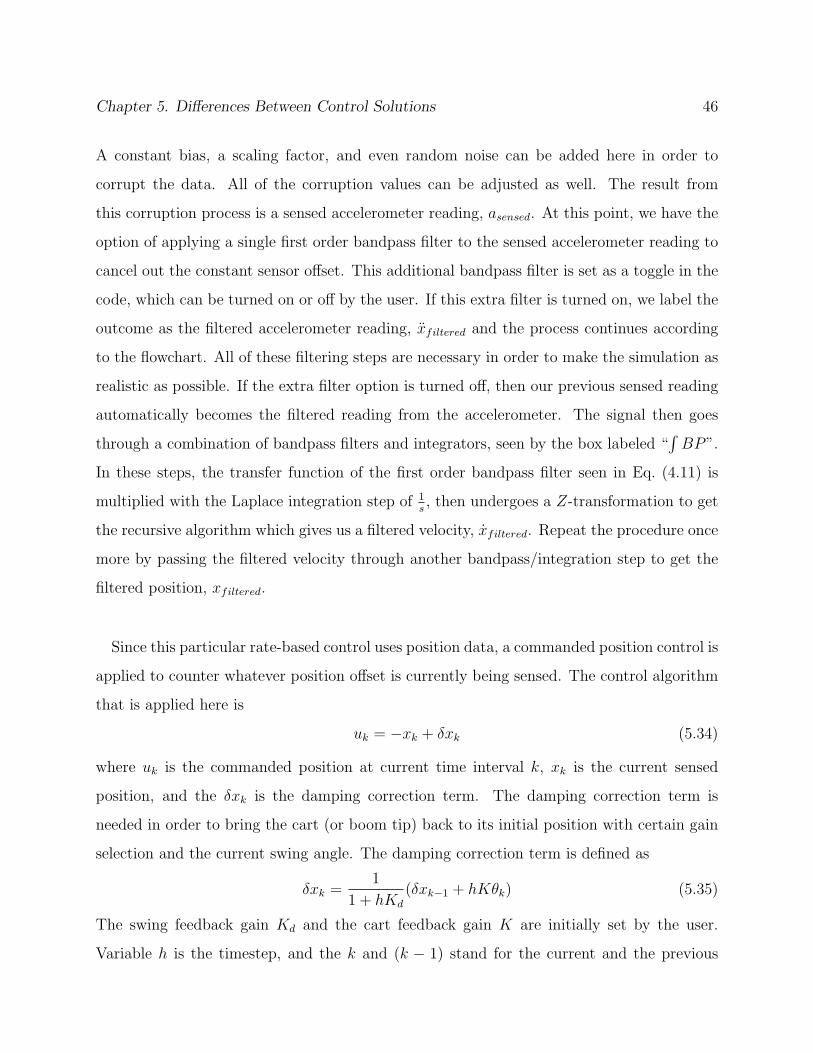
Chapter 5. Differences Between Control Solutions 46
A constant bias, a scaling factor, and even random noise can be added here in order to
corrupt the data. All of the corruption values can be adjusted as well. The result from
this corruption process is a sensed accelerometer reading, asensed. At this point, we have the
option of applying a single first order bandpass filter to the sensed accelerometer reading to
cancel out the constant sensor offset. This additional bandpass filter is set as a toggle in the
code, which can be turned on or off by the user. If this extra filter is turned on, we label the
outcome as the filtered accelerometer reading, xfiltered and the process continues according
to the flowchart. All of these filtering steps are necessary in order to make the simulation as
realistic as possible. If the extra filter option is turned off, then our previous sensed reading
automatically becomes the filtered reading from the accelerometer. The signal then goes
through a combination of bandpass filters and integrators, seen by the box labeled “∫BP”.
In these steps, the transfer function of the first order bandpass filter seen in Eq. (4.11) is
multiplied with the Laplace integration step of 1s, then undergoes a Z-transformation to get
the recursive algorithm which gives us a filtered velocity, xfiltered. Repeat the procedure once
more by passing the filtered velocity through another bandpass/integration step to get the
filtered position, xfiltered.
Since this particular rate-based control uses position data, a commanded position control is
applied to counter whatever position offset is currently being sensed. The control algorithm
that is applied here is
uk = −xk + δxk (5.34)
where uk is the commanded position at current time interval k, xk is the current sensed
position, and the δxk is the damping correction term. The damping correction term is
needed in order to bring the cart (or boom tip) back to its initial position with certain gain
selection and the current swing angle. The damping correction term is defined as
δxk =1
1 + hKd
(δxk−1 + hKθk) (5.35)
The swing feedback gain Kd and the cart feedback gain K are initially set by the user.
Variable h is the timestep, and the k and (k − 1) stand for the current and the previous

Chapter 5. Differences Between Control Solutions 47
time steps, respectively. The performance of the cart pendulum simulation is affected by
varying these two gain values, along with any changes in the initial angular conditions and
the length of the hoist cable. In our simulation, the selection of the gain values matches the
values that are in use in the actual crane PCS.
The control algorithm uses a commanded position value, u, to counter the changes in
position. However, our equations of motion in Eqs. (5.26 & 5.27) require both the current
real and commanded acceleration values. So successive differentiation steps are required by
passing the u to u using algorithm in Eq. (5.36) and from u to u using the algorithm in
Eq. (5.37).
u =1
h(uk − uk−1) (5.36)
u =1
h(uk − uk−1) (5.37)
The u term is the crane servo control because the commands sent by crane operator’s joystick
are in the form of velocity commands.
Now the equations of motion are computed with the availability of the initial angle θ,
angular rate θ, commanded acceleration u, and true acceleration x. Steps for solving the
equation of motion was described in Section 5.1.3 using Equations (5.12 to 5.17). Initially, the
starting conditions are specified by the user. After the first time step, every time step h from
that moment on relies on the conditions θ and θ of the previous time step. Also, it should
be noted that each time step h is divided into ten smaller time increments with changing
x(t) that represented the true acceleration at that instant. Yet, the u(t) that corresponds
to the time step h remains unchanged. The reason for having the control update ten times
faster than the simulation is to provide a more accurate true acceleration. The simulation
runs for a specified amount of time, which is also set by the user. The outcome is a series of
swing angles θ, and swing angule rates θ from each time step. The process continues until
the end of the user specified time frame. The MATLAB code can be seen in Appendix A.1.
Chapter 5. Differences Between Control Solutions 48
5.5 Simplified 1D Control Using Velocity Based In-
verse Kinematics
There are lots of similarities between the rate-based velocity control and the previous rate-
based position control. As mentioned before, the crane operator commands the crane using
velocity inputs. Therefore, by using the velocity based control algorithm, we can eliminate
one differentiation step, thus limiting errors and possibly yield equal if not better results.
As seen in the flowchart of Figure 5.3, the process starts just like the rate-based position
control with the true accelerometer data. The similarity continues through the corruption
phase, as well as the filtering/integration phase until the vfiltered output. Since this is a
control solution based on velocity, the vfiltered value goes into the controller in the following
equation
uk = −xk + δxk (5.38)
where the damping term (in its velocity form) keeps track of the cart’s position. The resulting
commanded velocity u is then differentiated into an acceleration and used in the equation of
motion, along with the true acceleration data and the angular rate. Basically, we still need
to integrate from the velocity to get a set of position values to be used within the controller
of Equation 5.38, we are simply reducing one differentiation step in the data manipulation
that feeds into the controller.
The hope is to eliminate any propagating error due to one less differentiation process. The
subsequent calculation of the Equation of Motion follows Equations (5.12 to 5.17) using the
fourth order Runge Kutta method.

Chapter 5. Differences Between Control Solutions 49
Figure 5.3: Flowchart of the Rate-Based Velocity Control
5.6 Summary
In this chapter we looked at the 3D inverse kinematic for the different types of controls.
Then we started with the derivation of the equation of motion using Lagrange’s Equation
for the cart pendulum system in order to simulate only the rolling motion of the ship. The
different types of simplified 1D control were the position-based control using IMU/GPS
system, the current rate-based position control that is implemented, as well as the new rate-
based velocity control. Next chapter presents some of the outputs that resulted from running
the simulation and the comparisons of different sensor performances.

Chapter 6
Results
On the market, there are numerous IMU sensors with varying specifications. The values
used in the simulations are based on the disturbance data from various IMUs. Trial simula-
tions are conducted to compare the effectiveness of the IMU-only control solutions, for both
the new position- and velocity-based crane control solutions.
6.1 Applying the Optional Filter
The use of the optional 1st order bandpass filter (Section 4.3.6) is designed to eliminate
the accelerometer sensed bias that exists. We run the test cases in the 1-D simulation to
see the effects of the filtering process. The first set of runs has the proposed extra filter
turned off, and then turned on for the second set of runs. In Figure 6.1, the first plot is the
acceleration plot with true and sensed values. For both on and off cases, an exaggerated
constant bias is used to make for easier viewing. The constant offset that results from the
bias is easily seen. Since the extra filter that would have cancelled this constant offset is not
available, the next plot is that of the true and the filtered velocity. Integration leads to the
function having one higher order. The bandpass filter cancelled that raised power, but the
50

Chapter 6. Results 51
initial constant offset is still noticeable. Same can be applied for transition from velocity to
the position plot.
Figure 6.1: Effects of Filtering Without Additional Filter in IMU-Based Control
Now we turn the extra filter on, which eliminates the constant offset from the bias from
the start. In Figure 6.2, we see in the first plot for acceleration that the offset exists between
the sensed and the true acceleration. However, it takes between 15 to 20 seconds for the
filtered acceleration to match the true acceleration as the red and the green lines overlap.
Having already cancelled the initial constant offset, the integration step raises the function

Chapter 6. Results 52
to the next power, but the bandpass filter eliminates any additional offsets. In the velocity
plots of Figure 6.2(b), the true and the filtered velocity match up after about 10 seconds.
Same can be said about integrating from velocity to position as it took 15 to 20 seconds for
the true and the filtered position signals to converge.
Figure 6.2: Effects of Filtering With Additional Filter in IMU-Based Control
The effects of the optional first order bandpass filter can also be seen in the performance of
the PCS. The differences of both the position- and velocity-based controllers each with the

Chapter 6. Results 53
optional filter turned on and off are shown in Figures 6.3 and 6.4, respectively. The plots
Figure 6.3: Effect of Optional Bandpass Filter in Rate-based Position Control
Figure 6.4: Effect of Optional Bandpass Filter in Rate-based Velocity Control
represent the location of the payload, in the form of the pendulum in our cart pendulum
simulation. Both figures have a constant bias in the beginning and takes approximately
20 seconds for the control to damp out the pendulation swing. The blue lines show the
cart pendulum behavior when the extra filter is off, and they show a 1m offset. The red
lines show a lack of a constant offset introduced by the initial bias, as its pendulation swing
reduces about the nominal position of 0m. This type of offset can show up in the form of our

Chapter 6. Results 54
aforementioned slow drifting frame. Over a matter of hours, the crane ship and ship docked
alongside of it may mirror the behavior of a constant offset by slowly drift away from the
nominal position. Such an error is easily correctable since there is a crane operator available.
That person simply has to manually adjust for the difference using the crane joystsick.
The PCS has its center frequency ωc of its filters set to match the period of the ship rolling
motion period. If the sensor’s center frequency deviates from the ship’s rolling motion period,
then the system is prone to phase leads and lag, and results in severe pendulation. However,
the actual PCS includes an updated center frequency that corresponds to the motion of the
ship in order to avoid such a problem.
6.2 Sweeps When Varying Different IMU Sensor Pa-
rameters
The ship and sensor parameters in the simulation are based on actual sensor data from
Table 6.1. As the sweep simulation conducts its runs, two chosen parameters vary. The
results of each run are shown in terms of a root mean square average of the residual oscillatory
motion of the payload. Each data on the plot represents an average payload position error
compare to the desired nominal position, after the removal of bias and initial transient effects.
The two varying parameters, along with their corresponding RMS error value, are recorded
and the entire sweep is presented in the form of contour plots.
The following test cases are the result of the cart pendulum simulation and is conducted
to see the sensitivity of the sensors when IMU sensor parameters, such as corruptions and
settings, are varied. The tests are run with the optional bandpass filter turned on and off to
see the differences caused by accelerometer’s constant offset. As seen in Figures 6.6 to 6.9,
the ship amplitude and the ship motion period are the two variables being swept. To clarify,

Chapter 6. Results 55
Table 6.1: List of Parameters Used in Cart-Pendulum Simulation
Parameter Value
Ship Motion Amplitude 1 m
Ship Motion Period 11 sec
Hoist Length 35 m
Time Step 1/40 sec
Period of the Filter Center Frequency ωo 11 sec
Filter Bandwidth BW 0.1 Hz
Filter Damping Coefficient ξ 0.707
Accelerometer Bias (Expensive) 2x10⁻³ g
Accelerometer Bias (Cheaper) 30x10−3 g
Scale Factor (Expensive) 1%
Scale Factor (Cheaper) 5%

Chapter 6. Results 56
the ship amplitude that is described here is the horizontal boomtip motion caused by rolling
motion of the crane ship. A sample correlation between the ship roll angle and horizontal
boomtip motion is seen in Figure 6.5 with various crane luff angles β. The crane boom
length is 37.5m, and we assume the base of the crane boom is approximately 20m off the sea
level.
Figure 6.5: Ship Rolling Angle vs Horizontal Boomtip Motion with Varying Luff Angle
From the sweeps of Figures 6.6 to 6.9, the velocity-based PCS of both the more expensive
and cheaper IMU performed better than the position-based solution in terms of their average
payload position error over a set period of time of 100 seconds. The velocity-based control
show improvements (in the average payload position error) of up to 1m in certain cases
compare to the same parameters in the position-based control. All of the velocity-based
control sweeps (rightside of Figures 6.6 to 6.9) have more blue region than the position-
based control sweeps (leftside of Figures 6.6 to 6.9). Higher average payload position error
means more pendulation swing. In all of the cases, as the amplitude of the ship rolling
motion increase, so does its average payload position error. Also, as the ship motion period
diverges from the center frequency of the bandpass filter (preset at a value of 11 seconds), the
average position errors increase–result in more pendulation swing. This behavior is expected
due to the phase lead or lag in the system when the pre-set center frequency of the filter and
the motion period are out of sync.
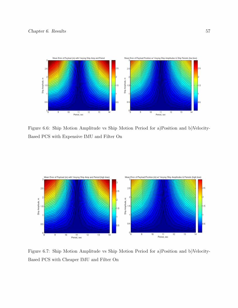
Chapter 6. Results 57
Figure 6.6: Ship Motion Amplitude vs Ship Motion Period for a)Position and b)Velocity-
Based PCS with Expensive IMU and Filter On
Figure 6.7: Ship Motion Amplitude vs Ship Motion Period for a)Position and b)Velocity-
Based PCS with Cheaper IMU and Filter On

Chapter 6. Results 58
Figure 6.8: Ship Motion Amplitude vs Ship Motion Period for a)Position and b)Velocity-
Based PCS with Expensive IMU and Filter Off
Figure 6.9: Ship Motion Amplitude vs Ship Motion Period for a)Position and b)Velocity-
Based PCS with Cheaper IMU and Filter Off
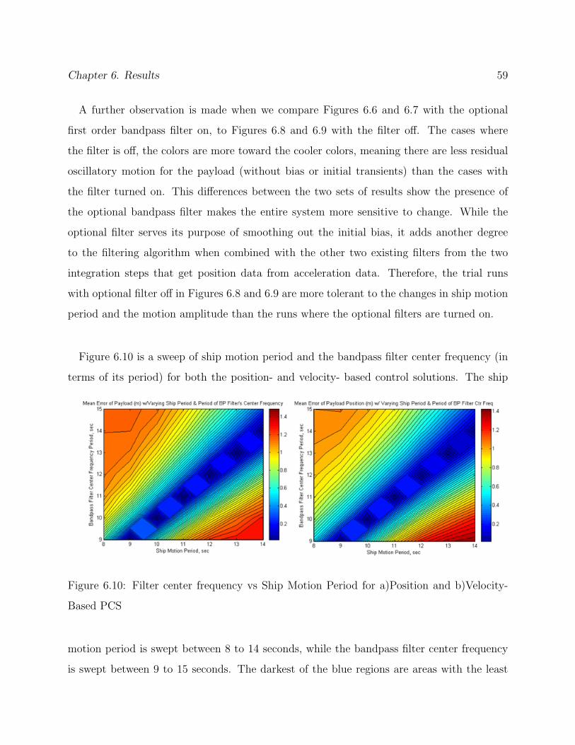
Chapter 6. Results 59
A further observation is made when we compare Figures 6.6 and 6.7 with the optional
first order bandpass filter on, to Figures 6.8 and 6.9 with the filter off. The cases where
the filter is off, the colors are more toward the cooler colors, meaning there are less residual
oscillatory motion for the payload (without bias or initial transients) than the cases with
the filter turned on. This differences between the two sets of results show the presence of
the optional bandpass filter makes the entire system more sensitive to change. While the
optional filter serves its purpose of smoothing out the initial bias, it adds another degree
to the filtering algorithm when combined with the other two existing filters from the two
integration steps that get position data from acceleration data. Therefore, the trial runs
with optional filter off in Figures 6.8 and 6.9 are more tolerant to the changes in ship motion
period and the motion amplitude than the runs where the optional filters are turned on.
Figure 6.10 is a sweep of ship motion period and the bandpass filter center frequency (in
terms of its period) for both the position- and velocity- based control solutions. The ship
Figure 6.10: Filter center frequency vs Ship Motion Period for a)Position and b)Velocity-
Based PCS
motion period is swept between 8 to 14 seconds, while the bandpass filter center frequency
is swept between 9 to 15 seconds. The darkest of the blue regions are areas with the least
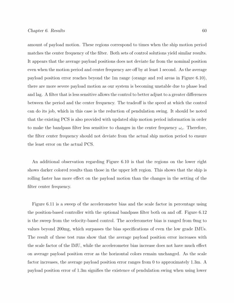
Chapter 6. Results 60
amount of payload motion. These regions correspond to times when the ship motion period
matches the center frequency of the filter. Both sets of control solutions yield similar results.
It appears that the average payload positions does not deviate far from the nominal position
even when the motion period and center frequency are off by at least 1 second. As the average
payload position error reaches beyond the 1m range (orange and red areas in Figure 6.10),
there are more severe payload motion as our system is becoming unstable due to phase lead
and lag. A filter that is less sensitive allows the control to better adjust to a greater differences
between the period and the center frequency. The tradeoff is the speed at which the control
can do its job, which in this case is the reduction of pendulation swing. It should be noted
that the existing PCS is also provided with updated ship motion period information in order
to make the bandpass filter less sensitive to changes in the center frequency ωc. Therefore,
the filter center frequency should not deviate from the actual ship motion period to ensure
the least error on the actual PCS.
An additional observation regarding Figure 6.10 is that the regions on the lower right
shows darker colored results than those in the upper left region. This shows that the ship is
rolling faster has more effect on the payload motion than the changes in the setting of the
filter center frequency.
Figure 6.11 is a sweep of the accelerometer bias and the scale factor in percentage using
the position-based controller with the optional bandpass filter both on and off. Figure 6.12
is the sweep from the velocity-based control. The accelerometer bias is ranged from 0mg to
values beyond 200mg, which surpasses the bias specifications of even the low grade IMUs.
The result of these test runs show that the average payload position error increases with
the scale factor of the IMU, while the accelerometer bias increase does not have much effect
on average payload position error as the horizontal colors remain unchanged. As the scale
factor increases, the average payload position error ranges from 0 to approximately 1.3m. A
payload position error of 1.3m signifies the existence of pendulation swing when using lower

Chapter 6. Results 61
Figure 6.11: Cart Pendulum Sweep Analysis of Scale Factor vs Bias in Position-based Control
with Optional Bandpass Filter a)Off, b)On
Figure 6.12: Cart Pendulum Sweep Analysis of Scale Factor vs Bias Velocity-based Control
with Optional Bandpass Filter a)Off, b)On

Chapter 6. Results 62
grade IMU sensors. When comparing both Figures 6.11 and 6.12 side-by-side, we see (based
on the amount of blue/light blue regions) that the use of the optional first order bandpass
filter in the beginning of the simulation yields similar data than if the filter is not used. This
result makes sense because this sweep compares only the scale factor and the bias, and the
bias are rejected for the most part through the filtering process. Meanwhile, the setting of
the center frequency is still close to the rolling motion period for these runs. However, as seen
in Chapter 3, the cost of an IMU inversely corresponds to its scale factor value. Therefore,
one should be aware that even though the filters can eliminate the bias, a high scale factor
can still drive up the payload position error and swing during payload transfer.
6.3 Summary
In this section, plots and sweeps from the cart pendulum simulation were presented to
show the workings of the additional bandpass filter, and the sensitivity of the sensors. Along
with the comparison between the position and velocity based control solutions using IMU.

Chapter 7
Conclusion
A focused analysis of an existing PCS is conducted using a cart pendulum model sim-
ulation. The cart pendulum simulation helps to narrow down to a one dimensional study
regarding the rolling motion of the crane ship during cargo transfer maneuvers to reduce its
pendulation swing. The modular nature of the program allows the changing of variables in
crane states, as well as sensor parameters. The simulation can then be swept to generate a
contour plot detailing two ranges of variables, as well as an average payload position error
from a nominal point that indicates the amount of swing.
We simulate two control solutions based solely on an IMU-only system using both position-
and velocity- based controllers. Results show that the optional bandpass filter in the new
control solutions work as expected in rejecting the constant bias in the accelerometer while
being more sensitive due to the presence of a higher order filter process. Therefore, the cases
without the optional filter show about the same level or performance in certain conditions,
and slightly better performance in more extreme conditions because a lower-ordered filters are
more robust. This study also shows the velocity-based control solution provides comparable
if not better results than the position-based solution. Both methods are sensitive to the
difference between the ship motion period and the center frequency of the bandpass filter.
63

Chapter 7. Conclusion 64
Lastly, it is shown that the bias of an accelerometer is not a large source of disturbance as
compared to scale factor due to the fact that the bias can be filtered out. Therefore, a low
grade IMU sensor is not recommended due to its high scale factor error. A mid-level quality
IMU sensor may be the best option due to the combination of its cost and the amount of
scale factor error it has.

Bibliography
[1] Vaughers, T. and Mardiros, M., “Joint Logistics Over the Shore Operation in Rough
Seas,” Naval Engineers Journal, May 1997, 385–393.
[2] Robinett,III, et al., “Pendulation Control System and Method for Rotary Boom
Cranes,” U.S. Patent No. 6,442,439, August 27, 2002.
[3] Bird, D., “Motion Compensation For Offshore Container Handling”, Naval Coastal
System Center, Panama City, FL, February, 1986.
[4] Aquino, M., Rodrigues, S., Dodson, A., Moore, T., and Waugh, S., “Results of Statisti-
cal Analysis of GPS Ionospheric Scintillation Data in Northern Europe 13–15 October
2003, Matera, Italy”, Institute of Engineering Surveying and Space Geodesy, The Uni-
versity of Nottingham, October 2003.
[5] http://www.FreeFoto.com, 2006.
[6] Priolo, Gary., “NavSource Naval History”, www.navsource.org/archives/09/76/
09760502.jpg, 2005.
[7] Pike, John., “GlobalSecurity.org”, www.globalsecurity.org/military/systems/ship/
images/3LCU-TACS.jpg, 2006.
[8] Evans, John, “T-ACS/RoboCrane Suspended Cargo Acquisition and Stabilization,”
Intelligent Systems Division, NIST, 1996.
65

Bibliography 66
[9] Naud et al. “Integrated and Automated Control of a Crane’s Rider Block Tagline Sys-
tem,” U.S. Patent No. 6,039,193, Mar. 21, 2000.
[10] Robinett, III et al. “Pendulation Control System and Method for Rotary Boom Cranes,”
U.S. Patent No. 6,442,439, Aug. 27, 2002.
[11] SmartCrane, LLC. www.smartcrane.com, 2006.
[12] Sakawa, Y., Shindo, Y., and Hashimoto, Y. “Optimal control of a rotary crane,” Journal
of Optimization Theory and Applications, 1981, pp.535-557.
[13] Takeuchi, S., Fujikawa, H., and Yamada, S., “The application of fuzzy theory for a rotary
crane control,” in Proceedings of the International Conference on Industrial Electronics,
Control, and Instrumentation: IECON 93, Lahaina, HI, Vol.1, pp.230-235.
[14] Sakawa, Y. and Nakazumi, A., “Modeling and control of a rotary crane,” Journal of
Dynamic Systems, Measurement, and Control, 1985, pp.200-206.
[15] Nguyen, H.T. and Laman, J., “Robust control of an overhead crane,” in Control 95
Melbourne, Australia, Vol.1, 1985, pp.235-238.
[16] Gustafsson, T., “Modeling and control of a rotary crane,” in Proceedings of the 3rd
European Control Conference: ECC 95, Rome, Italy, 1995, pp.3805-3810.
[17] Chin, C., Nayfeh, A., and Mook, D., “Dynamic and control of ship-mounted cranes,”
in Proceedings of the 39th Structures, Structural Dynamics, and Materials Conference,
Long Beach, CA, AIAA-98-1731.
[18] Abdel-Raman, E and Nayfeh, A., “Feasibility of two-dimensional control for ship-
mounted cranes,” in DETC2001 Proceedings of the ASME Design Engineering Technical
Conference, Pittsburgh, PA, DETC2001/VIB-21454.
[19] Nayfeh, et al., “Nonlinear Active Control of Dynamical Systems,” U.S. Patent No.
6,631,300, Oct. 7, 2003.

Bibliography 67
[20] Belsterling, Charles, “Stabilized Shipboard Crane,” U.S. Patent No. 4,932,541, June 12,
1990.
[21] Lee, Donald, “Automated All-Weather Cargo Transfer System,” U.S. Patent No.
5,154,561, Oct. 13, 1992.
[22] Holland, Carl, “Cable Array Robot for Material Handling,” U.S. Patent No. 6,826,452,
Nov. 30, 2004.
[23] Lawrence, A., Modern Inertial Technology: Navigation, Guidance and Control, Springer-
Verlag New York, Inc., New York, NY, 2nd Ed., 1998.
[24] Yazdi,N., Farrokh A., and Khalil N., “Micromachined Inertial Sensors,” Proceedings of
IEEE, Vol.86 No.8, August 1998, pp.1640-1659.
[25] Appalanix Corp. http://www.applanix.com/products/posmv index.php, 2006.
[26] Hide, C., T. Moore, M. Smith, “GPS and Low Cost INS Integration Using Commercial
Off-the-Shelf Components,” University of Nottingham, 2004.
[27] Ogata, K., System Dynamics, Prentice-Hall, Inc., Upper Saddle River, NJ, 3rd Ed.,
1998.
[28] http://www.dsptutor.freeuk.com/dfilt1.htm
[29] Parker, G.G., R. Robinett, B. Driessen, and C. Dohrmann, “Operator-in-the-loop con-
trol of rotary cranes,” in Proceedings of the 1996 International Society for Optical Engi-
neering Symposium on the Smart Structures and Materials; Industrial and Commercial
Applications of Smart Structure Technologies, Feb. 1996, vol. 2721, pp.364-372.
[30] Burden, R. and J. Faires, Numerical Analysis, Brooks/Cole, Pacific Grove, CA, 7th Ed.,
2001.
[31] Schaub, H. and J. Junkins, Analytical Mechanics of Space Systems, AIAA Educational
Series, Reston, VA, 2003.

Appendix A
MATLAB Codes
A.1 Main Program
%PROGRAM NAME: cp3.m
%ASSOCIATED FILES: TrueShipAccel3.m, SensedShipAccel3.m,
% FilteredShipVel3.m, FilteredShipMotion3.m, OneDShipAccel.m
% BPincp3.m, FilteredShipVel3i.m
%xddtrue -> xddsensed -> (xddfiltered ->) xdfiltered -> xfiltered
clear all
global L g h BW wo SF bias_value
%Sample Inputs
A = 1; Pd =11; L = 35; %Amplitude (m), Period (s), Hoist length (m)
t0 = 0; tfinal = 180; %t(0) and final time (s)
theta0 = 0; thetaDot0 = 0; %theta(0) (rad), theta-dot(0) (rad/s)
h = 1/40; %Timestep (s)
K = 14.828; %Gain (to stabilize pendulum swing)
Kd = 0.1669; %Gain (to put back to original position)
Transient_CUT = 30; %Amount of transient time to be discounted (s)
CutOut = Transient_CUT/h; %Number of actual time steps eliminated
SF = 0; %Accelerometer’s Scaling Factor
BW = 2*pi*(.1); %bandwith 2*pi*Hz=(rad/s)
wo = 2*pi*(1/11); %cutoff/center frequency 2*pi/Pd (rad/s)
DEG2RAD = pi / 180;
g = 9.81;
68

Appendix 69
back = 1; %a counter of sorts
BP_Switch = 0; %switch to turn on 3rd BP filter (0=off,1=on)
bias_value = 0.0015; %Sensor bias
%Initialize arrays
last_value = 1/h*tfinal+1+back;
X1 = zeros(1,last_value); %theta
X2 = zeros(1,last_value); %theta_dot
u = zeros(1,last_value);
udot = zeros(1,last_value);
udotdot = zeros(1,last_value);
dx = zeros(1,last_value);
xddtrue = zeros(1,last_value); %true acceleration data
xddsensed = zeros(1,last_value); %sensed acceleration data
xdfiltered = zeros(1,last_value); %filtered velocity data
xfiltered = zeros(1,last_value); %filtered x-position data
xtrue=zeros(1,last_value); %TESTING ONLY, true position
xdtrue=zeros(1,last_value); %TESTING ONLY, true velocity
utrue=zeros(1,last_value);
%Set initial conditions
X1(1,1:2) = theta0 * DEG2RAD; %set theta(0)
X2(1,1:2) = thetaDot0 * DEG2RAD; %set theta_dot(0)
[xddtrue xdtrue xtrue] = TrueShipAccel3(tfinal, A, Pd);
%*****MANIPULATE GAUSSIAN HERE******
[xddsensed] = SensedShipAccel3(tfinal, xddtrue);
if (BP_Switch == 1) %if switch is on, add 3rd BP filter
xddfiltered = zeros(1,last_value); %if switch is on, start xddfiltered
[xddfiltered] = BPincp3(tfinal, xddsensed);
[xdfiltered] = FilteredShipVel3i(tfinal,xddfiltered);
else if (BP_Switch == 0)
[xdfiltered] = FilteredShipVel3(tfinal, xddsensed);end
end
[xfiltered] = FilteredShipMotion3(tfinal, xdfiltered);
dx(1,1) = K*h*X1(1,1); %initialize delta_x term
i = 2;
for t = t0:h:tfinal

Appendix 70
dx(1,i) = 1/(1+h*Kd)*(dx(1,i-1) + K*h*X1(1,i));
u(1,i) = -xfiltered(1,i) + dx(1,i); %Current pendulation ctrl sys
udot(1,i) = (u(1,i) - u(1,i-1))/h;
udotdot(1,i) = (udot(1,i)-udot(1,i-1))/h; %Perfect drive system
%Runge Kutta Start
a = t; b = t + h;
m = 2; %represents 2 eqns in the system
h1 = (b-a)/10; %divide each run in 10 sections
N = (b-a)/h1; %# of increments
alpha(1) = X1(1,i); %current initial conditions
alpha(2) = X2(1,i);
t_temp = a;
for j = 1:m
w(j) = alpha(j);
end
for p = 1:N
TimeInc = t_temp; %from OneDShipAccel.m
xdotdot = OneDShipAccel(A,Pd,TimeInc); %acc @ true time increment
k(1,1)=h1*w(2);
k(1,2)=h1*(-(xdotdot + udotdot(i)) / L * cos(w(1)) - g / L ...
* sin(w(1)));
w1_new = w(1)+0.5*k(1,1);
w2_new = w(2)+0.5*k(1,2);
t_new = t_temp + h1/2;
TimeInc = t_new;
xdotdot = OneDShipAccel(A, Pd, TimeInc);
k(2,1) = h1*w2_new;
k(2,2) = h1*(-(xdotdot + udotdot(i)) / L * cos(w1_new) ...
- g / L * sin(w1_new));
w1_new = w(1)+0.5*k(2,1);
w2_new = w(2)+0.5*k(2,2);
t_new = t_temp + h1/2;
TimeInc = t_new;
xdotdot = OneDShipAccel(A, Pd, TimeInc);
k(3,1) = h1*w2_new;

Appendix 71
k(3,2) = h1*(-(xdotdot + udotdot(i)) / L * cos(w1_new) ...
- g / L * sin(w1_new));
w1_new = w(1)+k(3,1);
w2_new = w(2)+k(3,2);
t_new = t_temp + h1;
TimeInc = t_new;
xdotdot = OneDShipAccel(A, Pd, TimeInc);
k(4,1) = h1*w2_new;
k(4,2) = h1*(-(xdotdot + udotdot(i)) / L * cos(w1_new) ...
- g / L * sin(w1_new));
w(1) = w(1) + (k(1,1)+2*k(2,1)+2*k(3,1)+k(4,1)) / 6;
w(2) = w(2) + (k(1,2)+2*k(2,2)+2*k(3,2)+k(4,2)) / 6;
t_temp = a + p*h1;
end %Runge Kutta ends
if (i <= length(xddtrue) - 1) %Stopping point
X1(1,i+1) = w(1); %Store value for graphing
X2(1,i+1) = w(2);
utrue(1,i+1) = utrue(1,i) + udot(1,i)*h;
i = i + 1;
else
break
end
end
%To reduce data by PREVIOUSLY SPECIFIED TIME
counter = CutOut; %The new starting time [time steps]
for c1 = 1:(last_value-CutOut)
New_Theta(c1) = xfiltered(counter)+u(counter)+L*sin(X1(counter));
counter = counter + 1;
end
%To find the root mean squared error
Ideal_Result = 0; %Payload’s position difference that we want
Total_Diff = 0; %This variable to track of sum of differences
nn = length(New_Theta);
%RMS, SQUARE each term, AVG of squares, SQRT of the avg
for iii = 1:nn
Local_Diff = (New_Theta(iii)-Ideal_Result)^2;
Total_Diff = Local_Diff + Total_Diff;

Appendix 72
end
MeanError = sqrt(1/nn*Total_Diff);
fprintf(’RMS Error of payload’’s position difference = %f meters’,MeanError)
%%PLOTTING%%%
figure
plot([t0:h:tfinal+h], xddtrue, ’r’)
hold on
plot([t0:h:tfinal+h], xddsensed)
legend(’True Accel’,’Sensed Accel’)
if (BP_Switch == 1)
plot([t0:h:tfinal+h], xddfiltered, ’g’) %only if extra BP is on
legend(’True Accel’,’Sensed Accel’,’Filtered Accel’)
end
xlabel(’Time, t (sec)’)
ylabel(’Ship Acceleration (m/s^2)’)
title(’Ship Acceleration Comparisons’)
hold off
figure
plot([t0:h:tfinal+h], xdfiltered)
hold on
plot([t0:h:tfinal+h], xdtrue, ’r’)
legend(’Filtered Velocity’,’True Velocity’)
xlabel(’Time, t (sec)’)
ylabel(’Velocity (m/s)’)
title(’Ship Velocity Comparison’)
hold off
figure
plot([t0:h:tfinal+h], xfiltered)
hold on
plot([t0:h:tfinal+h], xtrue,’r’)
legend(’Filtered Position’,’True Position’)
xlabel(’Time, t (sec)’)
ylabel(’Ship Position, (m)’)
title(’Ship Position Comparison’)
hold off
%
% figure
% plot([t0:h:tfinal+h], X1(1,:)*180/pi,’o’)

Appendix 73
% xlabel(’Time, t (sec)’)
% ylabel(’Pendulum Swing Angle, \theta (deg)’)
% title(’Pendulum Swing Angle vs Time’)
% grid on
%
% figure
% plot([t0:h:tfinal+h], xfiltered(1,:)+u(1,:)+L*sin(X1(1,:)))
% xlabel(’Time, t (sec)’)
% ylabel(’Payload Position Difference, (m)’)
% title(’Difference in Payload Position vs Time’)
% grid on
%
% figure
% plot([t0:h:tfinal+h], xfiltered)
% hold on
% plot([t0:h:tfinal+h], u, ’r’)
% legend(’Ship Motion’, ’Ctrl Motion’) %Ideally should reflect each other
% xlabel(’Time, t (sec)’), ylabel(’Motion in X-Direction (m)’)
% title(’Comparison of Ship Motion and the Control Motion Against It’)
figure %%%NOT NEED TO BE PLOTTED ALL THE TIME%%%
plot(xfiltered(1,:)+u(1,:)+L*sin(X1(1,:)), L*cos(X1(1,:)),’go’)
%axis([-10,10,0,35]) %Set axis
set(gca,’XDir’,’default’, ’YDir’, ’reverse’) % reverse y axis
xlabel(’x Position (m)’)
ylabel(’y Position (m)’)
title(’Inertial Position of Pendulum’)
hold on
plot(xfiltered(1,1)+u(1,1)+L*sin(X1(1,1)), L*cos(X1(1,1)),’k*’) %start
plot(xfiltered(1,last_value)+u(1,last_value)+L*sin(X1(1,last_value)), ...
L*cos(X1(1,last_value)),’r*’) %end point
legend(’Pendulum Path’, ’Start Point’, ’End Point’)
%Graph in x vs. t
figure
%plot([t0:h:tfinal+h], xfiltered(1,:)+u(1,:)+L*sin(X1(1,:)),’go’)
plot([t0:h:tfinal+h], xtrue(1,:)+u(1,:)+L*sin(X1(1,:)),’go’)
%axis([-10,10,0,35]) %Set axis
%set(gca,’XDir’,’default’, ’YDir’, ’reverse’) % reverse y axis
xlabel(’Time t (sec)’)
ylabel(’Payload(Cart) x-Position (m)’)
title(’Cart Position vs Time’)

Appendix 74
hold on
% plot(xfiltered(1,1)+u(1,1)+L*sin(X1(1,1)), L*cos(X1(1,1)),’k*’) %start
% plot(xfiltered(1,last_value)+u(1,last_value)+L*sin(X1(1,last_value)), ...
L*cos(X1(1,last_value)),’r*’) %end point
% legend(’Pendulum Path’, ’Start Point’, ’End Point’)
A.2 Function Files
%FUNCTION NAME: TrueShipAccel3.m
function [xddtrue,xdtrue,xtrue] = TrueShipAccel3(tfinal, A, Pd)
global h
t = 0:h:tfinal+h;
xddtrue = -4*A*pi^2*sin(2*pi/Pd*t)/Pd^2;
xdtrue = 2*A*pi*cos(2*pi*t/Pd)/Pd;
xtrue =A*sin(2*pi*t/Pd);
%FUNCTION NAME: SensedShipAccel3.m
%A function that adds noise to the ship acceleration. Represents sensed
% data from instrument
function [xddsensed] = SensedShipAccel3(tfinal, xddtrue)
global h g bias_value SF
t = 0:h:tfinal+h;
%noise = 0; %Default noise function
bias = bias_value*g; %units m/s^2
%Start of Gaussian:
u1 = 0; %Initial value
N = length(t); %Number of terms/trials
mean = 0; sigma = 0.00*g; %Mean, noise(m/s^2)
noise = zeros(1,N); %Initialize matrix
for j = 1:N
for i = 1:6
u1 = u1 + rand(1);
end
u1 = u1 - 3;

Appendix 75
noise(1,j) = mean + sigma * u1;
u1 = 0; %Reset u1 variable
end
%End Gaussian
Scaling_Factor = 1+SF; %Scaling Factor. 1.005 = 0.5%SF
xddsensed = bias + Scaling_Factor*xddtrue;
%FUNCTION NAME: FilteredShipVel3.m
%A function that integrates xsensed doubledot to xsensed dot, and also adds
%in a filter.
function [xdfiltered] = FilteredShipVel3(tfinal, xddsensed)
global h BW wo xi
t = 0:h:tfinal+h;
length = 1/h*tfinal+1+1;
xdfiltered(1,1:2)=xddsensed(1,1:2);
%1st order bandpass and integrator
for q = 3:1:length
Term1 = xdfiltered(1,q-1)*(8-2*h^2*wo^2);
Term2 = xdfiltered(1,q-2)*(-4+2*BW*h-h^2*wo^2);
Term3 = xddsensed(q)*BW*h^2;
Term4 = xddsensed(q-1)*2*BW*h^2;
Term5 = xddsensed(q-2)*BW*h^2;
xdfiltered(1,q) = 1/(4+2*BW*h+h^2*wo^2)*(Term1+Term2+Term3+Term4+Term5);
end
%FUNCTION NAME: FilteredShipMotion3.m
%A function that takes the filtered ship velocity, and integrates to turn it
%into filtered ship motion to be used in main program
function [xfiltered] = FilteredShipMotion3(tfinal, xdfiltered)
global h BW wo xi
t = 0:h:tfinal+h;

Appendix 76
length = 1/h*tfinal+1+1;
xfiltered(1,1:2)=xdfiltered(1,1:2);
%1st order bandpass and integrator
for q = 3:1:length
Term1 = xfiltered(1,q-1)*(8-2*h^2*wo^2);
Term2 = xfiltered(1,q-2)*(-4+2*BW*h-h^2*wo^2);
Term3 = xdfiltered(q)*BW*h^2;
Term4 = xdfiltered(q-1)*2*BW*h^2;
Term5 = xdfiltered(q-2)*BW*h^2;
xfiltered(1,q) = 1/(4+2*BW*h+h^2*wo^2)*(Term1+Term2+Term3+Term4+Term5);
end
%FUNCTION NAME: BPincp3.m
function [xddfiltered] = BPincp3(tfinal, xddsensed)
global h BW wo xi
t = 0:h:tfinal+h;
length = 1/h*tfinal+1+1;
%1st order bandpass (don’t need integrator)
xddfiltered(1,1:2) = xddsensed(1,1:2);
for q = 3:1:length
Term1 = xddfiltered(1,q-1)*(8-2*h^2*wo^2);
Term2 = xddfiltered(1,q-2)*(-4+2*BW*h-h^2*wo^2);
Term3 = 2*h*BW*(xddsensed(q)-xddsensed(q-2));
xddfiltered(1,q) = 1/(4+2*BW*h+h^2*wo^2)*(Term1+Term2+Term3);
end