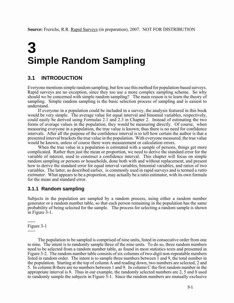
3-1

Source: Frerichs, R.R. Rapid Surveys (in preparation), 2007. NOT FOR DISTRIBUTION

3Simple Random Sampling3.1 INTRODUCTION

Everyone mentions simple random sampling, but few use this method for population-based surveys.Rapid surveys are no exception, since they too use a more complex sampling scheme. So whyshould we be concerned with simple random sampling? The main reason is to learn the theory ofsampling. Simple random sampling is the basic selection process of sampling and is easiest tounderstand.

If everyone in a population could be included in a survey, the analysis featured in this bookwould be very simple. The average value for equal interval and binomial variables, respectively,could easily be derived using Formulas 2.1 and 2.3 in Chapter 2. Instead of estimating the twoforms of average values in the population, they would be measuring directly. Of course, whenmeasuring everyone in a population, the true value is known; thus there is no need for confidenceintervals. After all the purpose of the confidence interval is to tell how certain the author is that apresented interval brackets the true value in the population. With everyone measured, the true valuewould be known, unless of course there were measurement or calculation errors.

When the true value in a population is estimated with a sample of persons, things get morecomplicated. Rather then just the mean or proportion, we need to derive the standard error for thevariable of interest, used to construct a confidence interval. This chapter will focus on simplerandom sampling or persons or households, done both with and without replacement, and presenthow to derive the standard error for equal interval variables, binomial variables, and ratios of twovariables. The latter, as described earlier, is commonly used in rapid surveys and is termed a ratioestimator. What appears to be a proportion, may actually be a ratio estimator, with its own formulafor the mean and standard error.

3.1.1 Random sampling

Subjects in the population are sampled by a random process, using either a random numbergenerator or a random number table, so that each person remaining in the population has the sameprobability of being selected for the sample. The process for selecting a random sample is shownin Figure 3-1.

-----Figure 3-1-----

The population to be sampled is comprised of nine units, listed in consecutive order from oneto nine. The intent is to randomly sample three of the nine units. To do so, three random numbersneed to be selected from a random number table, as found in most statistics texts and presented inFigure 3-2. The random number table consists of six columns of two-digit non-repeatable numberslisted in random order. The intent is to sample three numbers between 1 and 9, the total number inthe population. Starting at the top of column A and reading down, two numbers are selected, 2 and5. In column B there are no numbers between 1 and 9. In column C the first random number in theappropriate interval is 8. Thus in our example, the randomly selected numbers are 2, 5 and 8 usedto randomly sample the subjects in Figure 3-1. Since the random numbers are mutually exclusive

3-2

(i.e., there are no duplicates), each person with the illustrated method is only sampled once. Asdescribed later in this chapter, such selection is sampling without replacement. -----Figure 3-2-----

Random sampling assumes that the units to be sampled are included in a list, also termed asampling frame. This list should be numbered in sequential order from one to the total number ofunits in the population. Because it may be time-consuming and very expensive to make a list of thepopulation, rapid surveys feature a more complex sampling strategy that does not require a completelisting. Details of this more complex strategy are presented in Chapters 4 and 5. Here, however,every member of the population to be sampled is listed.

3.1.2 Nine drug addicts

A population of nine drug addicts is featured to explain the concepts of simple random sampling.All nine addicts have injected heroin into their veins many times during the past weeks, and haveoften shared needles and injection equipment with colleagues. Three of the nine addicts are nowinfected with the human immunodeficiency virus (HIV). To be derived are the proportion who areHIV infected (a binomial variable), the mean number of intravenous injections (IV) and shared IVinjections during the past two weeks (both equal interval variables), and the proportion of total IVinjections that were shared with other addicts. This latter proportion is a ratio of two variables and,as you will learn, is termed a ratio estimator. -----Figure 3-3-----

The total population of nine drug addicts is seen in Figure 3-3. Names of the nine male addictsare listed below each figure. The three who are infected with HIV are shown as cross-hatchedfigures. Each has intravenously injected a narcotic drug eight or more times during the past twoweeks. The number of injections is shown in the white box at the midpoint of each addict. Withone exception, some of the intravenous injections were shared with other addicts; the exact numberis shown in Figure 3-3 as a white number in a black circle.

Our intention is to sample three addicts from the population of nine, assuming that the entirepopulation cannot be studied. To provide an unbiased view of the population, the sample meanshould on average equal the population mean, and the sample variance should on average equal thepopulation variance, corrected for the number of people in the sample. When this occurs, we canuse various statistical measures to comment about the truthfulness of the sample findings. Toillustrate this process, we start with the end objective, namely the assessment of the population meanand variance.

Population Mean. For total intravenous drug injections, the mean in the population is derived usingFormula 3.1

(3.1)

where Xi is the total injections for each of the i addicts in the population and N is the total numberof addicts. Thus, the mean number of intravenous drug injections in the population shown in Figure3-3 is

3-3

or 10.1 intravenous drug injections per addict.

Population Variance. Formula 3.2 is used to calculate the variance for the number of intravenousdrug injections in the population of nine drug addicts.

(3.2)

where σ2 is the Greek symbol for the population variance, Xi and N are as defined in Formula 3.1and is the mean number of intravenous drug injections per addict in the population. UsingFormula 3.2, the variance in the population is

Sample Mean. Since the intent is to make a statement about the total population of nine addicts,a sample of three addicts will be drawn, and their measurements will be used to represent the group.The three will be selected by simple random sampling. The mean for a sample is derived usingFormula 3.4.

(3.4)

where xi is the number of intravenous injections in each sampled person and n is the number ofsampled persons. For example, assume that Roy-Jon-Ben is the sample. Roy had 12 intravenousdrug injections during the past two weeks (see Figure 3-3), Jon had 9 injections and Ben had 10injections. Using Formula 3.4,

the sample estimate of the mean number of injections in the population (seen previously as 10.1) is10.3.

Sample Variance. The variance of the sample is used to estimate the variance in the populationand for statistical tests. Formula 3.5 is the standard variance formula for a sample.

(3.5)

where s2 is the symbol for the samplevariance, xi is the number of

intravenous injections for each of the i addicts in the sample and is the mean intravenous drug

3-4

injections during the prior week in the sample. For the sample Roy-Jon-Ben with a mean of 10.3,the variance is

3.2 WITH OR WITHOUT REPLACEMENT

There are two ways to draw a sample, with or without replacement. With replacement means thatonce a person is selection to be in a sample, that person is placed back in the population to possiblybe sampled again. Without replacement means that once an individual is sampled, that person is notplaced back in the population for re-sampling. An example of these procedures is shown in Figure3-4 for the selection of three addicts from a population of nine. Since there are three persons in thesample, the selection procedure has three steps. Step one is the selection of the first sampled subject,step two is the selection of the second sampled subject and step three is the selection of the thirdsampled subject. In sampling with replacement (Figure 3-4, top), all nine addicts have the sameprobability of being selected (i.e., 1 in 9) at steps one, two and three, since the selected addict isplaced back into the population before each step. With this form of sampling, the same person couldbe sampled multiple times. In the extreme, the sample of three addicts could be one person selectedthree times.-----Figure 3-4-----

In sampling without replacement (WOR) the selection process is the same as at step one )that is each addict in the population has the same probability of being selected (Figure 3-4, bottom).At step two, however, the situation changes. Once the first addict is chosen, he is not placed backin the population. Thus at step two, the second addict to be sampled comes from the remaining eightaddicts in the population, all of whom have the same probability of being selected (i.e., 1 in 8). Atthe third step, the selection is derived from a population of seven addicts, with each addict havinga probability of 1 in 7 of being selected. Once the steps are completed, the sample contains threedifferent addicts. Unfortunately, the reduced selection probability from the first to the third step isat odds with statistical theory for deriving the variance of the sample mean. Such theory assumesthe sample was selected with replacement. Yet in practice, most simple random samples are drawnwithout replacement, since we want to avoid the strange assumption of one person being tallied astwo or more. To resolve this disparity between statistical theory and practice, the variance formulasused in simple random sampling are changed somewhat, as described next.

3.2.1 Possible samples With Replacement.

When drawing a sample from a population, there are many different combinations of people thatcould be selected. Formula 3.6 is used to derive the number of possible samples drawn withreplacement,

(3.6)

where N is the number in the total population and n is the number of units being sampled. Forexample when selecting three persons from the population of nine addicts shown in Figure 3-3, thesample could have been Joe-Jon-Hall, or Sam-Bob-Nat, or Roy-Sam-Ben, or any of many othercombinations. To be exact, in sampling with replacement from the population shown in Figure 3.3,there are

3-5

or 729 different combinations of three addicts that could have been selected.

-----Figure 3-5-----

The frequency distribution of the mean number of IV drug injections of the 729 possible samplesselected with replacement is shown in the top section of Figure 3-5. Notice that the distribution hasa bell shape, similar to a normal curve. There are three notable features of these 729 possiblesamples.

Notable feature one. While the range of the 729 possible sample means is from a low of 8 to a highof 12, the average value of the sample means for the intravenous drug injections during the priorweek is 10.1, the same as the population mean calculated previously with Formula 3.1. That is,when sampled with replacement, on average the sample mean provides an unbiased estimate of thepopulation mean. Notable feature two. The average variance of the 729 possible samples of three selected withreplacement is equal to the population variance of the nine drug addicts (see Formula 3.2), as shownin Formula 3.7

(3.7)

where is the variance of sample i, where i goes from 1 to 729, the total number of possiblesamples when selecting three from nine with replacement. Notable feature three. For random samples of size n selected from an underlying population withreplacement, the variance of the mean of all possible samples is equal to the variance of theunderlying population divided by the sample size. For the 729 possible samples, the averagevariance of the mean for a sample of three from an underlying population of nine is shown inFormula 3.8.

(3.8)

Thus with this form of sampling, on average the variance of the sample mean provides an unbiasedestimate of the variance of the population divided by the sample size.

Given these three features – namely that the mean, sample variance, and variance of the samplemean are unbiased estimators of the mean, population variance, and variance of the populationdivided by the sample size – it would seem that sampling with replacement is very useful. But issuch sampling usually done?

Without Replacement. In the realistic world of sampling, subjects are typically not included inthe sample more than once. Also, the order in which subjects are selected for a survey is notimportant (that is, Roy-Sam-Ben is considered the same as Sam-Ben-Roy). All that matters is if thesubject is in or out of the sample. Hence in most surveys, samples are selected disregarding orderand without replacement. But does sampling without replacement provide unbiased estimators ofthe population mean and variance? The answer is “yes,” but needing some additionalmodifications, to be presented next.

Formula 3.9 is used to calculated the number of possible samples that can be drawn without

3-6

replacement, disregarding order,

(3.9)

where N is the number of people in the population, n is the number of sampled persons, and ! is thefactorial notation for the sequential multiplication of a number times a number minus 1, continuinguntil reaching 1. That is, N! (termed "N factorial") is N times N-1 times N-2 and the like with thelast number being 1.

In our example, we are selecting without replacement and disregarding order a sample ofthree addicts from a population of nine addicts (see Figure 3-3). Using Formula 3.9, we find thereare

or 84 possible samples. Fortunately when using Formula 3.9, all factorial numbers do not have tobe multiplied. For example, the 9! in the numerator can be converted to 9 x 8 x 7 x 6!, and the 3! x(9-3)! in the denominator can be converted to 3 x 2 x 1 x 6!. By dividing 6! in the numerator by 6!in the denominator to get 1, the formula is reduced to 9 x 8 x 7 divided by 3 x 2 x 1 or 84 possiblesamples.

The distribution of all possible sample means for the 84 samples selected with replacement,disregarding order in shown in the bottom section of Figure 3-5, below the distribution of the 729possible sample means selected with replacement. Are the two distributions similar? It is hard totell since the scale does not permit an easy visual comparison. Figure 3-6 shows the same twodistributions, but as a percentage of the total number of possible samples (i.e., 729 with replacementand 84 without replacement). -----Figure 3-6-----

There are two things to notice. First, the mean of all possible samples selected with replacement(i.e., 10.1) is equal to the mean of all samples selected without replacement, and both sample meansare equal to the population mean. Thus, the sample mean on average remains an unbiased estimatorof the population mean when sampling without replacement. Second, the percentage distributionsof those selected with and without replacement are similar in shape, but there are fewer outlyingsamples among those sampled without replacement. That is, there is less variability among the 84possible samples selected without replacement than the 729 possible samples selected withreplacement. The reduced variability in sampling without replacement is addressed in two ways,namely with a change in the variance formula for the population variance and in the addition of afinite population correction factor (FPC).

First, different from Formula 3.2, the population variance that is being estimated by the samplevariance when sampling without replacement has a different denominator (N-1), as shown inFormula 3.10.

(3.10)

where S2 is the modified population variance and Xi, N and are as defined previously. For thepopulation of nine drug addicts, the modified variance is

3-7

When sampling without replacement the average variance of all 84 possible samples is equal to themodified population variance (see Formula 3.11).

(3.11)

where si2 is the variance in sample i, with i going from 1 to 84, the total number of possible samples

when selecting three from nine without replacement. Second, the variance of the sample mean of all 84 possible samples when sampling without

replacement is equal to the modified population variance divided by the sample size (as mentionedin notable feature three in sampling with replacement) times a correction factor that accounts forthe shrinkage in variance. This correction factor, termed the finite population correction (FPC) isshown in Formula 3.12.

(3.12)

where N is the size of the population and n is the size of the sample. In samples where the samplesize is large in relation to the population (an example being a sample of three from a population ofnine), the FPC reflects the reduction in variance that occurs when sampling without replacement(i.e., with 84 possible samples in the example) compared to sampling with replacement (i.e., with729 possible samples in the example). This reduction in variability when sampling withoutreplacement was observed in Figure 3.6, and in the comment that there were fewer outliers in thewithout replacement group.

For the 84 possible samples, the average variance of the mean for a sample of three from anunderlying population of nine is shown in Formula 3.13.

(3.13)

Notice that n/N is the fraction of the population that is sampled. Therefore the FPC is oftendescribed by sampling specialists as "one minus the sampling fraction." Notice also that thevariance of the average samples mean is 0.36 for sampling without replacement compared to 0.48(see Formula 3.8) when sampling with replacement, resulting in smaller estimates of sampling errorand greater efficiency in the sampling process when the sampling fraction is large. Finally, note thatif the sampling fraction is very small, as occurs in typical rapid surveys of few persons drawn froma large population, then the finite population FPC term reduces to approximately 1, and is no longerneeded.

In summary, when sampling without replacement (i.e., the more practical and typical form ofsampling) there are also three notable features, related but not entirely the same as stated earlier inthe section on sampling with replacement. Notable feature one. When sampled without replacement, on average the sample mean providesan unbiased estimate of the population mean. This feature is the same whether sampling with orwithout replacement. Notable feature two. The average variance of all possible samples selected without replacement isequal to the modified population variance (i.e., N -1 rather than N in the denominator as when

3-8

sampling with replacement – see Formula 3.2 versus 3.10).Notable feature three. For random samples of size n selected without replacement from anunderlying population, the variance of the mean of all possible samples is equal to the modifiedvariance of the underlying population divided by the sample size, multiplied by the finite populationcorrection (FPC) factor.

These three features account for the ability on average of samples selected with replacementto truthfully describe an underlying population, and to provide statistical measures of random errorin the sampling process.

In conclusion, what has been presented so far is that when drawing a simple random samplefrom a population, the selected sample is only one among many possible samples. Yet if the sampleis selected in an unbiased manner, the average value of all possible samples is the same as the truevalue in the population. Since the true value is not know and only one sample is being selecting,the variability in the sampling process needs to be described, providing a measure of possiblerandom error. Finally, when sampling without replacement the variability of all possible samplemeans is less than the variability of the sample means when selecting samples with replacement,especially when the sampling fraction is large. This reduction in variance is accounted for by theFPC term and results in greater efficiency in the sampling process, but only when the samplingfraction is large. As mentioned in Chapter 2, we will be using formulas that describe the variabilityof all possible samples to derive a confidence interval for the sample mean or proportion.

In the following sections we will continue to sample three addicts, again drawn withoutreplacement from a population of nine addicts. This time, however, a more extensive set offormulas will be used to calculate the mean and variance of two equal interval variables, a binomialvariable and a ratio estimator.

3.3 AVERAGE VALUE AND STANDARD ERROR

Every population to be sampled has a true value for the variable of interest. A sample is drawn fromthe population to estimate this true value. This sample could be viewed as a selection of units froma population of units. Or it could be viewed as the selection of one sample from a population of allpossible samples. In this section, we will determine the distribution of all possible samples for fourvariables: total injections, shared injections, HIV infection, and the ratio of shared to totalinjections. We will derive the mean, standard error and confidence interval for all possible samplesof three addicts sampled without replacement from the nine addicts (see Figure 3-3). Since thesample is drawn without replacement, there are 84 possible samples.

3.3.1 Equal Interval Data

Each addict in the population of nine injected himself with drugs multiple times during the past twoweeks. Some of the injections were shared with other addicts. The total number of injections andthe number of shared injections are both equal interval variables, as described in Chapter 2.Different from binomial variables, equal intervals variables have many outcomes ranging in equalintervals from 0 to the upper end of a scale.

Total Injections. The first of the two equal interval variables to be analyzed is total intravenousdrug injections. The data are shown in white squares for each addict in Figure 3-3. As noted usingFormula 3.1, the mean number of intravenous injections per addict in the population of nine drugaddicts is

or 10.1 injections per addict. The distribution of the total injections in the population of nine addictsis shown in Figure 3-7.

3-9

-----Figure 3-7-----

With the small population of nine, there are 84 possible samples of three addicts that could beselected, assuming sampling without replacement and disregarding order. To be derived for eachpossible sample are the mean for total injections (termed variable x) , the standard error of the meanand the confidence interval for total injections. The mean of each of the 84 possible samples iscalculated with Formula 3.4. The one sample of Joe-Hal-Roy serves as an example.

-----Figure 3-8-----

The distribution of the 84 possible sample means is shown in the upper left of Figure 3-8. Theaverage value of the 84 possible sample means is 10.1, the same as the mean for the total populationof nine addicts (see Figure 3-7). Thus, the sampling scheme for total injections is consideredunbiased. Observe, however, that some of the possible sample means had values as low as 9injections while others had values as high as 11.5 injections. By chance alone we could haveselected one of these outlying samples, even though the sampling scheme is unbiased.

The top right of Figure 3-8 shows the distribution of the standard errors of 84 sample means.To calculate each standard error, the variance of the sample mean is derived using Formula 3.14.

(3.14)

As noted earlier, the term (N-n)/N in Formula 3.14 is the finite population correction, included onlybecause this is a sample selected without replacement. For the sample Joe-Hal-Roy, the varianceof the sample mean is

The standard error of the total injections, , is the square root of the variance, , as shownin Formula 3.15.

(3.15)

For the sample Joe-Hal-Roy, the standard error is

A confidence interval can be created for each of the 84 possible samples using Formula 3.16.

(3.16)where is as defined previously and t is the value of Student’s t that corresponds to a specified

3-10

level of confidence (usually 95%) and a sample size of three. But why use a t-value whenconfidence intervals are typically derived with z-values, also termed the “standard normal deviate?” -----Figure 3-9-----

The t-value is appropriate here because of the exceptionally small size of the sample. Asobserved in Figure 3-9, for a normal-sized simple random sample of 200 or more, the t-value isidentical to the z-value. For a 95% confidence interval, the z-value is 1.96. Yet with a small sampleof three, the t-value for a 95% confidence interval is 4.30, far greater than 1.96. Using Formula3.16, the 95% confidence interval for the mean of total injections of 10.0 estimated in the sampleJoe- Hal-Roy is

or a lower limit of 5.9 and an upper limit of 14.1. The 84 confidence intervals for all possible samples are shown in the bottom section of Figure

3-8. Five of the 84 possible samples do not bracket the true value (marked with an asterisk at thebottom of the figure) , while 79 (i.e., 94%) do bracket the true value. Keep in mind that only oneof the 84 possible samples is selected for the survey. Seventy-nine times out of 84, the constructedconfidence interval will contain the true value. Thus in advance of sampling, we can be 94%confident that the interval we construct would contain the true value, assuming the sample wasselected in an unbiased manner. If the sample and population had both been much larger, a 95%confidence interval using the z-value of 1.96 would have been constructed rather than the 94%confidence interval for 84 possible samples of three with the t-value of 4.30.

Shared Injections. The second of the two equal interval variables is shared intravenous druginjections. Here the letter y is used to describe the statistics rather than x as with total injections.Both of these variables will be used in a subsequent section for calculating a ratio estimator. Thusthey are identified with different letters, even though the mathematical calculations are identical. -----Figure 3-10-----

The data for shared injections are shown in black circles in Figure 3-3, while the distributionof the shared injections in the population of nine addicts is shown in Figure 3-10. The population mean for the shared intravenous injections is calculated using Formula 3.17.

(3.17)

Here is the mean value of variable Y in the population, Yi is the value of variable Y in person i, Nis the number of persons in the population . The mean number of shared intravenous injections peraddict in the population of nine drug addicts is

3-11

As before, there are 84 possible samples. For each is derived the mean, standard error of themean and 95% confidence interval. The mean number of shared injections for each sample of threeis calculated with Formula 3.18

(3.18)

where is the mean number of intravenous injections per addict in the sample, yi is the number ofshared injections per sampled addict, and n is the number of sampled addicts. Continuing with theexample of Joe- Hal- Roy, the mean number of shared injections is

-----Figure 3-11-----

The distribution of the 84 possible sample means is shown in the upper left of Figure 3-11.The average value of the 84 possible sample means is 3.0, identical to the mean for the totalpopulation of nine addicts. Thus, the sampling scheme for shared injections is unbiased. Of course,most of the 84 possible samples have mean values different from 3.0, although the average of allpossible samples is the same as the true value of 3.0.

The distribution of the standard errors of the 84 sample means is observed in the upper rightof Figure 3-11. The standard errors are derived by first calculating the variance of the sample mean,v(y), using Formula 3.19.

(3.19)

The finite population correction, (N-n)/N, reduces the size of the variance when sampling withoutreplacement. For the sample of Joe- Hal-Roy, the variance of the sample mean for shared injectionsis.

The standard error of the total injections, , is the square root of the variance, . For thesample Joe-Hal-Roy, the standard error is the square root of 0.96 or 0.98.

The confidence interval for the sample Joe- Hal- Roy for the mean of shared injections of 4.33is

or a lower limit of 0.12 and an upper limit of 8.54. The 84 confidence intervals for all possiblesamples are shown in the bottom section of Figure 3-11. Five of the confidence intervals do notbracket the true value in the population and are marked with an asterisk. Since 79 (94%) of the 84

3-12

possible samples do bracket the true value, the confidence limits in the small example populationare actually for 94% confidence intervals. Of course for the one sample that we selected, we wouldnot know if it is among the group of five that do not contain the true interval or 79 that do. Afterthe sample is drawn and an interval is created, the probability is either 0 or 1 that the intervalcontains the true value. That is, the confidence interval either does or does not bracket the truevalue. Before the sample is drawn, however, we can be 94% confident that the interval to becalculated will bracket the true value. For larger samples and larger populations, the z-value of 1.96would be used instead to derive intervals which bracket the true value 95 percent of the time.

3.3.2 Binomial Data

The values for binomial data are derived in a similar manner to equal interval data, although theformulas appear slightly different. The binomial variable being considered is HIV infection, avariable with two outcomes, 0 if not infected and 1 if infected. In the population shown in Figure3-3, three of the nine addicts were infected with HIV. Using Formula 3.1, the mean HIV status inthe population of nine drug addicts is

or 0.33 as presented as a proportion or 33 as a percentage. The mean value of the variable HIVinfection with an outcome of 0 or 1 is the same as the proportion who are HIV positive. That is, themean of a binomial variable coded with a 0-1 outcome is the proportion with the attribute. Themean of a binomial variable is also defined as

(3.20)

where P is the proportion in the population, A is a count of those with the attribute of interest, andN is the number of units in the population. In our example, there are three HIV infected persons ina population of nine addicts. Thus the proportion in the population that is infected is 3/9 or 0.33.-----Figure 3-12-----

The distribution of HIV status for the nine addicts is shown in Figure 3-12. When a binomial variable such as HIV status is coded 0 or 1, Formulas 3.1 and 3.20 are the

same. If a binomial variable is coded 1 or 2, however, then the mean value derived with Formula3.1 will be different than the proportion calculated with Formula 3.20. For the mean of a binomialvariable to appear as a proportion (or as a percentage if multiplied by 100), the outcome must becoded as 0 or 1, or tallied as a count of those with the attribute.

Next we calculate the proportion that is infected with HIV for each of the 84 possible samplesof three addicts. Formula 3.21 is used to calculate the proportion for each sample.

(3.21)

where p is the proportion that is HIV positive in the sample, a is the count of HIV infected personsin the sample, and n is the number of sampled addicts. Thus for the sample of Joe- Hal-Roy, theproportion that is HIV positive is

3-13

If by chance this sample would have been selected, the estimate of the proportion who are HIVpositive would have been twice the true value of 0.33. -----Figure 3-13-----

The distribution of the 84 possible sample proportions is shown in the upper left of Figure 3-13. The average value of the 84 possible sample proportions is 0.33, the same as the proportion forthe total population of nine addicts. When the average value of all possible samples is equal to theproportion (or mean for equal interval variables) in the population, we say that the sampling schemeis unbiased. Notice, however, that being unbiased does not imply that the proportion for the onesample being selected is the same as the proportion in the population. Instead being unbiasedindicates that on average the sample proportion equals the population proportion. Also notice thatsome of the possible sample proportions had values as low as 0 while others had values as high as1. Thus by chance alone, the sample being selected could have a proportion far different from thetrue value of 0.33. In fact, only with 45 of the 84 possible samples was the point estimate of theproportion the same as the true value.

Due to the small size of the population and even smaller size of the sample, the proportion inthe example does not behave as would occur in a larger population and larger sample. Here 20 ofthe 84 possible samples have a value of 0 and 1 has a value of 1. The consequence of having a meanvalue of 0 or 1 will become apparent when calculating the variance, standard error and confidenceintervals for the proportion, which follows next.

The variance of a proportion for a simple random sample, selected without replacement, iscalculated using Formula 3.22,

(3.22)

where v(p) is the variance of the sample proportion, p is the sample proportion, and n is the numberof sampled addicts. For the sample of Joe- Hal-Roy, the variance of the proportion is

The standard error of the sample proportion, is the square root of the sample variance, asshown in Formula 3.23.

(3.23)

For the sample Joe- Hal-Roy, the standard deviation is the square root of 0.074 or 0.272. With this example of a sample of three from a population of nine, Figure 3-13 shows that there

are only four outcomes for the sample proportion, namely 0/3, 1/3, 2/3 or 3/3. For those 20possible samples with a proportion of 0, the variance of the proportion is the same as for the onesample with a proportion of 1, namely

3-14

In both instances, with a variance of 0 the se(p) is 0. Thus for 21 of the 84 possible samples, thestandard error of the proportion in the small example is 0. For the remaining 63 possible samplesthe proportion was either 1/3 or 2/3, both having the same variance.

For these 63 possible samples, the standard error of the proportion is

Thus with a sample of three from a population of nine, there are only two values for the se(p),namely 0 or 0.272, as shown in the upper right of Figure 3-13. Such limited values for a binomialvariable do not occur when the population and samples are larger, as occurs with typical rapidsurveys. Nevertheless, the example remains useful for demonstrating the calculations.

Using the standard error, the confidence intervals are calculated for each of the 84 possiblesamples. The confidence interval is derived using Formula 3.24.

(3.24)

where p is the proportion, se(p) is the standard error and t is a statistic corresponding to the z-valuewith the sample is exceptionally small, as noted in Figure 3-9.

To calculate 95% confidence intervals for each of the 84 possible samples, we use a t-valueof 4.30, much larger than a z-value of 1.96 typically used with 95% confidence intervals. Theconfidence interval for the sample Joe- Hal-Roy with a proportion 0.67 is

or a lower limit of 0 and an upper limit of 1. Unfortunately, because the sample of three is so small,the confidence interval is extremely wide, and hence is of little use, other than to demonstrate thecalculations. The 84 confidence intervals are shown in the bottom of Figure 3-13. With such asmall sample, most of the confidence intervals are very wide, extending from 0 to 1. In 21 of the84 samples the standard error was 0. For these 21 samples, the confidence interval did not bracket0.33, the true proportion in the population. The 21 samples are identified in Figure 3-23 with anasterisk. It is clear from viewing Figure 3-13 that for this small sample of three addicts drawn froma population of nine addicts, only a 75% confidence interval could be derived. That is in 63 timesout of 84 (75%), the surveyor would be confident that the created interval brackets the true value.For larger surveys with billions and trillions of possible samples, 95% of the confidence intervalsthat would be derived using a z-value of 1.96 would bracket the true value in the sampledpopulation, assuming there was no bias in the sample selection.

3.3.3 Ratio Data

What comes next is a different way of viewing the data, introduced earlier in Chapter 2. Rather thatconsidering the mean number of injections or the mean number of shared injections, we willdetermine the proportion of injections that were shared. This proportion is actually a ratio of tworandom variables: shared injections (variable y) and total injections (variable x). Notice that thesample is of addicts, not injections. Thus the three addicts in the sample may have different numbersof shared injections (one variable) and of total injections (a second variable). Yet the sample is onlycomprised of three addicts. Later in this chapter you will learn the difference between the units thatare sampled, given here as addicts, and the units that are analyzed, namely total and sharedinjections. The former are termed sampling units while the latter are elementary units.

3-15

-----Figure 3-14-----

When considering injections rather than people, the data can be viewed as in Figure 3-14. Theratio of the two variables “shared” to “total” is calculated with Formula 3.25.

(3.25)

where R is the ratio of variable Y to X in the population, Yi is the value of variable Y in person i, Xiis the value of variable X in person i, N is the number of persons in the population, and G is the sumsymbol indicating to add the values for each person from 1 to N. -----Figure 3-15-----

As shown in Figure 3-15, there were 27 shared injections during the past two week and 91 totalinjections, for a true ratio in the population of 0.297. Notice that the ratio is given as a proportion,but a proportion of injections, not of people.

The ratio of shared to total injections is calculated for each of the 84 possible samples usingFormula 3.26.

(3.26)

For the sample Joe- Hal- Roy, the ratio estimator (that is, our estimate of the ratio) is calculated as

Notice that this is an estimate of the proportion of injections that is shared. The number could alsobe multiplied times 100 to derive the percentage of injections that are shared (i.e., 43%). -----Figure 3-16-----

The ratio for the 84 possible samples is shown in the upper left of Figure 3-16. Here the meanof all possible sample ratios is slightly different from the ratio in the total population. While thedifference is small (that is, 0.297 in the population versus 0.296 in mean of all possible samples),there is a difference nevertheless. Ratio estimators may be slightly biased, so that the average of allpossible samples is not the same as the true ratio in the population. When the sample size is larger,however, the bias becomes minimal. The issue of bias in ratio estimators will be further addressedlater in this chapter.

Next the variance of the ratio for each of the 84 possible samples will be calculated, followedby the standard errors and confidence intervals. The variance formula is different from thosepresented earlier. The formula will be presented here, but will await Chapter 5 to be discussed in

3-16

more detail.

(3.27)

The finite population correction term in Formula 3.27 is (N-n)/N, the ratio in the sample is r, andthe other terms are as previously defined. For the sample Joe-Hal-Roy, the variance of the sampleratio is

The standard error of the ratio, se(r), is the square root of the variance, v(r) as shown in Formula3.28.

(3.28)

For the sample Joe-Hal-Roy, the standard error is the square root of 0.0055 or 0.074. Thedistribution of standard errors for all possible samples is shown in the upper right of Figure 3-16.

The confidence interval for the ratio, CI(r), is derived using Formula 3.29.

(3.29)

where se(r) is the standard error and t is the t-value for the stated sample size. For the sample Joe-Hal-Roy, the confidence interval is..

or a lower limit of 0.11 and an upper limit of 0.75. Confidence intervals for all 84 possible samplesare shown in the lower section of Figure 3-16. The vertical axis with “Ratio (Shared/Total)” extendsfrom a low of -0.4 to a high of 1.0, appropriate for a ratio but different from a proportion that goesfrom 0 to 1. While none of the point estimates of the sample ratios extend beyond 0 or 1, some ofthe confidence intervals do. This issue will be addressed in Figure 3-17. Also observe that 5 of the84 confidence intervals (6%) do not bracket the true value in the population. Thus 94% of theintervals enclosed the true value. The interpretation is that in advance of sampling, we can be 94%confident that intervals derived with Formula 3.29 would bracket the true value. With largersamples from larger populations, the confidence intervals created with Formula 3.29 , but using thez-value of 1.96, would bracket the true value 95 percent of the time, assuming of course that therewas no bias in the sample selection.

-----Figure 3-17-----

When doing rapid surveys, the analysis is often of a ratio estimator appearing as a proportion.That is, the ratio estimator seems like a variable with values between 0 and 1, even though in reality

3-17

the range could be much wider. Since the point estimate for a ratio estimator that acts like aproportion lies between 0 and 1, the problem lies with the confidence limits, both on the high andlow end. Since a proportion above 1 or below 0 does not make sense, the range of the confidencelimits in rapid surveys is typically truncated, as shown in Figure 3-17. Note that this truncation hasno effect on the confidence that the presented intervals bracket the true ratio in the population. 3.4 SAMPLES AND ELEMENTS

In the example of drug addicts, the starting point was a population of nine addicts from which threeaddicts were randomly selected. The process of sampling to identify the prevalence of HIVinfection is shown in Figure 3-18. In order to sample from the population of nine addicts, all mustfirst be assembled in a list termed a frame. From this frame, three units are sampled. Each unit istermed a sampling unit while the group of sampling units is termed the sample. In Figure 3-18, thesampling unit is a drug addict and the sample is three addicts. The units to be analyzed, termedelementary units, are drug addicts (or persons) and are the same as the sampling units. The groupof elementary units is referred to as elements. In this example, the sample is the same as theelements. That is, the group selected in the sample is the same as the group to be analyzed. InFigure 3-18, one addict is HIV positive and the other two are not. Thus the population prevalence(or proportion) is 1/3 or 0.33, the numerator being HIV infected addicts and the denominator beingsampled addicts. Because a sample of three addicts was selected, the size of the denominator isfixed as three. In estimating HIV prevalence, the numerator varies from one possible sample to thenext. That is, the denominator is fixed but the numerator is a random variable. -----Figure 3-18-----

A slightly different situation is shown in Figure 3-19. Here the sample is also three addictsbut the elements are nine injections. If the analysis is of the mean number of injections per addictor mean number of shared injections per addict, the derivation is the mean for an equal intervalvariable. While the denominator remains fixed at three addicts, the numerator varies from onepossible sample to the next. That is, the numerator is a random variable, but not the denominator.-----Figure 3-19-----

The elements can also be analyzed independent of the sample. Specifically, the number ofshared injections can be related to the number of total injections. This is a proportion, but usinginjections rather than persons. The denominator of the proportion is the number of injections whichvaries from one sample to the next, depending which addicts were included. In this proportion boththe numerator and denominator are random variables. As a result, the data are analyzed as a ratioestimator, or a ratio of one random variable to another. -----Figure 3-20-----

So what happens when the simple random sample is of households rather than of persons? InFigure 3-20 there is a population of households. To sample from this population, the householdsare arranged in a list or frame and households are sampled randomly from the frame. For thisexample, the sample consists of 30 households, selected randomly from the population of manyhouseholds. For the analysis, the interest is not in characteristics of the housing unit. Insteadinformation is wanted about the about the household occupants, namely people. Thus the analysisis of elements in the households, although only households were sampled. For such a survey, theanalysis is of a ratio estimator, or comparison of two random variables. The random variable in thedenominator is the number of persons in the sampled households and the random variable in thenumerator is the number of persons with the attribute being studied.

3-18

3.5 SURVEY OF SMOKING BEHAVIOR

In Section 3.3, the population to be sampled was addicts. Yet for one analysis ) shared to totalinjections ) the data were viewed as a ratio, although the results were presented as a proportion orpercentage. You observed in Figure 3-16 that a confidence interval can be created for a ratioestimator, although in our small example, the interval for some of the possible samples was verywide. You also noted in Figure 3-16 that there was a small bias in the ratio with the average valueof all possible samples (i.e., 0.296) being slightly different from the true value in the population (i.e.,0.297). This section will further explore ratio estimators, using a survey of smoking behavior toillustrate the various issues and principals. -----Figure 3-21-----

3.5.1 Sample of Persons

Before considering ratio estimators, assume that a sample of 90 persons was sampled by simplerandom selection from a population frame of 3,000 persons as shown in Figure 3-21. The intentis to determine the prevalence of current cigarette smoking behavior. Thus the sample units andelementary units are both persons and the outcome of the analysis is a binomial variable (i.e., smoker= 1, non-smoker = 0). In this population, 54% currently smoke. The sampling is done withreplacement, discarding order. Thus using Formula 3.9, the number of possible samples of 90 froma population 3,000 is,

a very large number of possible samples! For each of these possible, we could derive the mean,standard error and 95% confidence interval. Yet doing so would be a formidable task, and thecertainly the results could not be viewed graphically. Instead, the population is replicated in acomputer spreadsheet model, and 100 surveys of 90 persons each are randomly selected from theframe of all possible samples for graphic presentation. To derive the 95% confidence interval, the finite population correction term is included and a t-value of 1.986 is used instead of the z-valueof 1.96 (see Figure 3-9, sample size of 90). The 95% confidence interval for each of the 100 surveysis derived as (see Formulas 3.22 and 3.24),

with the 100 confidence intervals as shown in Figure 3-22.

-----Figure 3-22----- Observe that the average standard error for the 100 surveys is 5.2% which in later discussion willbe termed “medium variability.” The mean of the 100 samples was 53.1% smokers, nearly identicaland within random statistical variation of the 54% who smoked in the total population. Also noticethat five of the 100 confidence intervals did not bracket the true value of 54% in the population, aswould be expected when deriving 95% confidence intervals. Figure 3-22 will serve as acomparison, when next we consider a household survey with elementary units different fromsampling units.

3-19

3.5.2 Sample of Households

Assume that 30 households (HH) with an average of three persons per HH were drawn in a simplerandom sample from a population frame of 1,000 households. As previously shown in Figure 3-20,in such a survey the sampling unit of a household is different from the elementary unit of a person.In fact, in such surveys the people in a household are represented by two variables, the first beingthe existence of each person and the second being the smoking status of each person. Thus theproportion who smoke is derived as a ratio of two variables within the selected households, namelysmoking status and existing persons, and as such is a ratio estimator. When analyzing a ratioestimator, a slightly different variance formula is used (similar to Formula 3.27), to be furtherexplained in Chapter 5.

(3.30)

where N is the number of households in the population, n is the number of households in the sample,ai is the number who smoke in each household, p is the proportion who smoke in the total sample,mi is the number who exist in each household, and is the average number of persons perhousehold. -----Figure 3-23-----

Furthermore, the households in the population are of five occupancy sizes, as shown in Figure3-23. Each group in the population resides in 200 homes, and in the total population of 1,000households the average is three persons per household. Thus the simple random samples of personsand households have the same number of persons (i.e., 3,000), although in the household survey thepeople are distributed in 1,000 households.

Because the household survey is a sample of 30 households from a population of 1,000households, the number of possible samples is not as great as in when doing a simple random sampleof 90 persons from a population of 3,000 people. Again using Formula 3.9, the number of possiblesamples of 30 from a population 1,000 is,

still a huge number of possible samples. As before with the simple random sample of persons, acomputer spreadsheet model is used to randomly select and present 100 of the possible samples of30 households from the population of 1,000 households. The 95% confidence interval will againuse a t-value instead of the z-value used in larger rapid surveys, but this time of 2.0452 (see Figure3-9, sample size is 30). The 95% confidence interval for each of the 100 household surveys isderived as (see Formulas 3.22 and 3.24),

Variability of Smoking. Measures such as the variance, standard error and confidence intervalprovide a numeric assessment of the variability of smoking behavior in the population. In a simplerandom sample of persons, the variability is observed when comparing one individual to another.In contrast, the variability of persons in a simple random sample of households is expressed both

3-20

within households by the smoking patterns of the people that occupy the household, and betweenhouseholds, comparing the proportion of residents who smoke in one households versus the others.-----Figure 3-24-----

In Figure 3-22, the variability of the persons selected in a simple random sample was presentedas 100 different 95% confidence intervals and summarized with the average standard error value of5.2%. This level of variation was termed “medium variability.” Figure 3-24 shows two situationswhere the distribution of smoking behavior is the same in the population of 3,000 persons (the topsection) and in the 1,000 households (the bottom section). The only change in the bottom sectionis that households were placed around members of the population. Thus the people withinhouseholds are as variable in their smoking patterns as in the population. Or restated, the chanceof being a smoker within a household is independent of the smoking status of other members of thehousehold. This may not seem logical given human behavior, but instead is used to illustrate anotion. Since the level of variability in the population of 3,000 persons and 1,000 households withan average of three persons per household is the same, the household surveys should also exhibit“medium variability.” -----Figure 3-25----- The distribution of smokers within each group of 200 households is shown in Figure 3-25. Thefigure is divided into four sections, each describing the population household distributions that isassociated with different levels of smoking variability in random sample surveys. The firstdistribution to be considered is of medium variability in part B. Medium Variability. In this example, 54% of the population smokes. Assuming that people insmall households are just as likely to smoke as people in large households, then the percent smokersin each of the five-sized households should also be 54%. Figure 3-25 B shows the distribution ofsmokers in households by household size, for household surveys in which the variability is the sameas in a simple random sample of persons (i.e., medium variability).

-----Figure 3-26-----

When drawing 100 samples of 30 households from the billions of possible samples, the valuesof the 95% confidence intervals are presented in Figure 3-26 B. The dark horizontal line shows thetrue value in the population, or 54% smokers. Notice that the standard error of 5.1% is nearlyidentical to the standard error of 5.2% for the simple random sample (see Figure 3-22). The minordifference is due to random variation in the sampling process. The mean of the 100 samples is53.9%, very close to the true value of 54%. Finally, notice that six of the 100 confidence intervalsin Figure 2-26 B do not bracket the true value of 54% smokers from this population, nearly the sameas the five that would be expected by chance. If many more sets of 100 surveys would have beendrawn from all possible samples, the percentage of 95% confidence intervals that do not bracketthe true value would likely be in the 4-6 percent range, averaging 5 percent.

So far we have considered the situation where the level of variability in a household survey(termed “medium” in magnitude) is identical to a random sample of persons in the population. Whatif this is not true? What if the variability in a household survey is greater or less than the variabilityof a survey of persons? To understand the variability of household surveys, we need next toconsider variability both within households and between households.

3.5.1 Variability Within and Between Households

The variability of a binomial variable such as smoking is derived using variance formula for aproportion (see Formula 3.22). Leaving out the finite population correction term, the v(p) formula

3-21

is reduced to

This formula shows that for any given household size, the variance of the proportion who smoke isdepended on the size of the numerator, namely p x q, distributed as shown in Figure 3-27 for five-person households. -----Figure 3-27----- The variance within a five-person household will be zero if either none of the occupants are smokersor if all of the occupants are smokers. Conversely, the variance within households will be largestif either two or three of the five household members are smokers. -----Figure 3-28----- There are 200 five-person households in the total population. The variability within and betweenthese 200 households is shown in Figure 3-28 for the population with 54% smokers. If most of the200 households have high variability within households (i.e., namely have 2-3 smokers), then the200 households will be distributed by smoking status as in Figure 3-28, bottom left. That is, mostof the households will have 3 smokers, many will have 2 smokers, and a handful will have 4smokers. The variability of smokers in these 200 five-person homes is less (i.e., low variability)than the variability of the five-person homes in the previous example (i.e., medium variability), withvariability the same as in the general population, as seen in Sections A and B of Figure 3-25. Thesame principal of higher variability within households resulting in lower variability betweenhouseholds is also seen in Figure 3-5 A and B, comparing the one-, two-, three- and four-personhouseholds in the two sections.

The right section of Figure 3-28 presents a different situation. When five-person householdshave either no smokers or all smokers, the variance within households is zero (i.e., low variability).Yet, when all of the 200 households are split with about half having no smokers and approximatelyhalf having five smokers, the variance between households becomes very large (i.e., highvariability). Section C of Figure 3-25 shows the distribution of the five sets of 200 households whenthe variability is large.

These two graphs, Figures 3-25 and 3-28, illustrate a concept that is very important whenplanning rapid surveys. If the variable that is being considered (in our example it is “smoking”) isdistributed within households in a near random manner, then the variability of a household surveywill be nearly the same as the variability of a simple random sample of the population. If thevariable being studied is a highly infectious disease, then households might have either all personsinfected or no persons infected. In such situations, the variability would be low within householdsbut high between households. Finally, if the variable occurs uniformly in all households with halfof each household having the attribute and the other half not, then the variability will be high withinthe households but low between the households.

The effect of the variability between households on the 95% confidence interval derived fromthe household survey is shown in Figure 3-26. Section B provides the comparison group (“mediumvariability), or the same pattern for a household survey of 30 (with an average of three occupantsper household) as a simple random sample of 90 persons. When the variability is low withinhouseholds (i.e., either none or all having the attribute), Section C shows the 95% confidenceintervals became very wide, exhibiting high variability. Conversely, when about half the peoplewithin a household uniformly have an attribute and the variability between households is low,Section A shows very narrow 95% confidence intervals.

The proportion who smoke in Sections A-C of Figures 3-25 and 3-26 have three things incommon. First, the proportion is derived as a ratio estimator (i.e., ratio of two random variables).Second, the value of 54% who smoke in the underlying population of 1,000 households is the same

3-22

in each of five-sized groups of 200 households. That is, in Sections A-C of the two figures, thepercentage who smoking is not associated with household size, but rather is uniform by householdsize. Third, the 95% confidence intervals act as would be expected. That is, about 5 percent of the100 intervals do not bracket the true value in the population. In Section A of Figure 3-26, only four95% confidence intervals do not bracket 54%, while in Section B, six 95% confidence intervals donot bracket the true value. Finally in Section C, exactly five intervals do not bracket the true value.The difference between four, six and five non-bracketing intervals is due to chance variation in thesample of 100 surveys from the huge number of possible surveys, not due to an error in the statisticalcalculations.

But what happens if there is high variability (i.e., low variability within households and highvariability between households) and the percentage who smoke is associated with household size?The answer to this question is addressed in Section D of Figures 3-25 and 3-26. Here the variabilitybetween households is as extreme as in Section C. Yet while the percentage who smoke in the totalpopulation remains at 54%, the percentage who smoke in the various sized households rangesbetween 10% in one-person households and 80% in five-person households. This change addsfurther distortion to the calculation of the ratio estimator, but not enough to change the usefulnessof the 95% confidence intervals. As seen in Section D of Figure 3-26, the 95% confidence intervalsremain wide (as would be expected with high variability), but only five out of 100 of the intervalsdo not bracket 54%, the true value in the population. Thus the confidence intervals still behave asexpected. -----Table 3-1-----

The analyses of the four sets of household surveys (i.e., 30 households with an average of 3persons per household) presented in Sections A-D of Figures 3-25 and 3-26 are summarized in Table3-1, and compared to a simple random sample of 90 persons. The average standard error for theattribute “smoking” when compared to the surveys of 90 persons is lower in household surveys withlower variability between households, the same in household surveys with medium between-household variability, and much greater in household surveys with high variability. Increasing thebetween household variabiliy did not result in bias when the percentage who smoked was not relatedto household size, since the mean percent smokers was nearly the same as the 54% in the totalpopulation. When the situation was altered so that the percentage who smoked was associated withhousehold size, the ratio estimator of the proportion who smoked became biased, but only slightly(i.e., 52.8% versus 54%). While these observations are being made on a household survey drawnby simple random sample households, the same issues will later be addressed when considering thevariability in clusters, as done in two-stage cluster surveys. 3.6 SUMMARY

In this chapter you learned about simple random sampling and what happens when the sampling unitis different from the elementary unit. Two examples were featured: a sample of three drug addictsfrom a population of nine addicts, and a sample of 30 households from a population of 1,000households. You should understand how a simple random sample is selected, how the standard errorand confidence interval are calculated, and the interpretation of the confidence interval. The latteris especially important for explaining your findings to others who may not have much understandingof statistics. In addition, you have learned that certain variables must be analyzed differently in asurvey because they are not collected as sampling units. Instead they are elementary units that areassociated with, but different from, sampling units. When the elementary unit is the unit of interest,we analyze the findings as a ratio estimator. This point will be further discussed in Chapter 5.Finally, you learned that variability of an attribute within aggregated units such as householdseffects variability between households, and that this variability is reflected in the size of the surveyconfidence interval.

Coming in Chapter 4 is a presentation of equal probability of selection methods and the needto select samples for rapid surveys with probability proportionate to size.

3-23

Figure 3-1. Random sample of three units from apopulation of nine units.

Figure 3-2. Table of random numbers.

3-24

Figure 3-3. Population of nine intravenous drugaddicts.

Figure 3-4. Sample of three addicts from apopulation of nine addicts.

3-25

Figure 3-5. Distribution of all possible sample means with andwithout replacement (actual scale).

Figure 3-6. Distribution of all possible sample means with andwithout replacement (percentage scale).

3-26

Figure 3-7. Distribution of total intravenousinjections in a population of nine drug addicts.

Figure 3-8. Mean, standard error, and confidence interval for mean oftotal injections in all possible samples of three addicts from a populationof nine addicts. (* does not bracket true value)

3-27

Figure 3-9. Substitution of t-value for z- value in derivingconfidence interval for sample of three addicts.

Figure 3-10. Distribution of shared intravenousinjections in a population of nine drug addicts.

3-28

Figure 3-11. Mean, standard error, and confidence interval for mean ofshared injections in all possible samples of three addicts from a populationof nine addicts. (* does not bracket true value)

Figure 3-12. Distribution of HIV status in apopulation of nine drug addicts.

3-29

Figure 3-13. Proportion, standard error, and confidence interval forproportion with HIV in all possible samples of three addicts from apopulation of nine addicts. (* does not bracket true value)

Figure 3-14. Shared and total intravenous druginjections in a population of nine drug addicts.

3-30

Figure 3-15. Distribution of shared and totalintravenous drug injections in a population of ninedrug addicts.

Figure 3-16. Ratio, standard error, and confidence interval for ratio ofshared injections to total injections in all possible samples of three addictsfrom a population of nine addicts. (* does not bracket true value)

3-31

Figure 3-17. Confidence interval with range from 0 to 1 for ratio ofshared injections to total injections in all possible samples of three addictsfrom a population of nine addicts. (*does not bracket true value)

Figure 3-18. Sampling from population with sample (drugaddicts) same as elements (drug addicts).

3-32

Figure 3-19. Sampling from population with sample (drugaddicts) different from elements (injections).

Figure 3-20. Sampling from population with sample(households) different from elements (people).

3-33

Figure 3-21. Simple random sample of 90 persons from apopulation of 3,000 persons, analyzed for current smokingbehavior.

Figure 3-22. 95% confidence intervals for 100 random samples of 90persons from a population of 3,000 in which 54% are smokers. (* does notbracket true value)

3-34

Figure 3-23. Household survey of smoking behavior inpopulation with 1,000 households of five resident number,each group occupying 200 households.

3-35

Figure 3-24. Medium variability of smoking behavior isidentical in the sampling frames of 3,000 persons (top) and1,000 households occupied by an average of 3 persons(bottom).

3-36

Figure 3-25. Distribution and variability of smokers in 1,000 households (HH)by HH size (each has 200 HHs) in a population in which 54% are smokers. A-Ddescribed in text.

3-37

Figure 3-26. 95% confidence intervals for smoking status in 100 surveys of 30households by distribution and variability of smokers in population of 1000households. A-D described in text. (* does not bracket true value)

Figure 3-27. Variance of binomial variable“smoking” by number of smokers within five-person households.

3-38

Figure 3-28. High variability within households (HHs)results in low variability between HHs and lowvariability within HHs results in high variabilitybetween HHs. Smokers comprise 54% of thepopulation.

Table 3-1. Summary effects on standard error (SE) and mean in 100 simple randomsample (SRS) surveys of smoking behavior in population with 54% smokers.

Survey type

VariabilityMean (%)smokers* BiasBetween Within SE (%)

Persons§ -- -- 5.2 53.1 No

Households† Low High 3.5 53.9 No

Households† Medium Medium 5.1 54.1 No

Households† High Low 9.8 54.3 No

Households¶ High Low 9.8 52.8 Slight

* in 100 of all possible samples of either 90 persons or 30 households§ SRS of 90 persons in a population of 3,000 persons† SRS of 30 households in a population of 1,000 households, smokers (%) not associated

with household size¶ SRS sample of 30 households in a population of 1,000 households, smokers (%)

positively associated with household size