SIMPLE LINEAR REGRESSION AND CORRELATION Prepared by: Jackie Zerrle David Fried Chun-Hui Chung...

SIMPLE LINEAR REGRESSION AND CORRELATION

Prepared by:Jackie ZerrleDavid FriedChun-Hui ChungWeilai ZhouShiyhan ZhangAlex FieldsYu-Hsun ChengRoosevelt Moreno

AMS 572.1 DATA ANALYSIS, FALL 2007.

What is Regression Analysis?

A statistical methodology to estimate the relationship of a response variable to a set of predictor variables.

It is a tool for the investigation of relationships between variables.

Often used in economics – supply and demand. How does one aspect of the economy affect other parts?

Was proposed by German mathematician Gauss.

Linear Regression

The simplest relationship between x ( the predictor variable) and Y (the response variable) is linear.

is a random error with

represents the true but unknown mean of Y. This relationship is the true regression line.

0 1 , ( 1, 2,..., ).i i iY x i n

i 2( ) 0 and ( )i iE Var

0 1( )i i iE Y x

Simple Linear Regression Model

Simple Linear Regression Model

4 Basic Assumptions:

1. The mean of is a linear function of .

2. The have a common variance , which is

the same for all values of x.

3. The errors are normally distributed.

4. The errors are independent.

iY ix

2iY

i

i

Example -- Sales vs. Advertising--

Information was given such as the cost of

advertising and the sales that occurred as a

result.

Make a scatter plot

To get a good fit, however, we will use the Least

Squares (LS) method.

Example -- Sales vs. Advertising--Data

Sales($000,000s) ( ) Advertising ($000s) ( )

28 71

14 31

19 50

21 60

16 35

iy ix

Try to fit a straight line :

Where o = 2.5 and

Look at the deviations between the observed values and the points from the line:

0 1y x

128 14

3.571 31

0 1( ) ( 1, 2,..., )i iy x i n


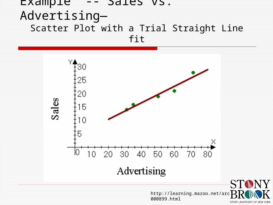
http://learning.mazoo.net/archives/000899.html

Example -- Sales vs. Advertising—Scatter Plot with a Trial Straight Line fit

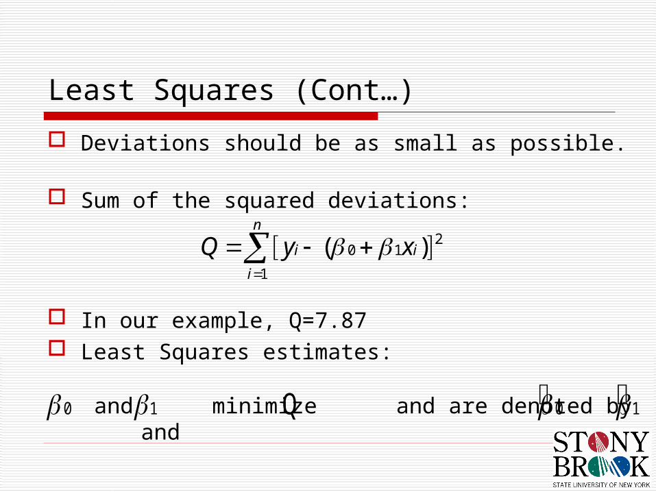
Least Squares (Cont…)

Deviations should be as small as possible.

Sum of the squared deviations:

In our example, Q=7.87 Least Squares estimates:

0 1 0 1 Q

20 1

1

( )n

i i

i

Q y x

and minimize and are denoted by and

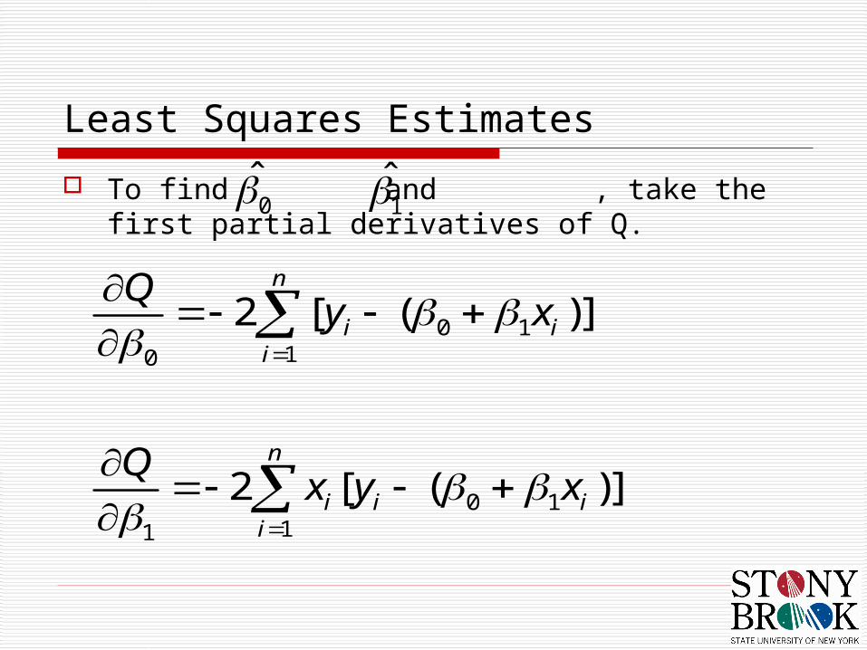
Least Squares Estimates

To find and , take the first partial derivatives of Q.

0

0 110

0 111

2 [ ( )]

2 [ ( )]

n

i ii

n

i i ii

Qy x

Qx y x

1

We then set these partial derivatives equal to zero and simplify.

These are our normal equations:

0 11 1

20 1

1 1 1

n n

i ii i

n n n

i i i ii i i

n x y

x x x y

Normal Equations

Normal Equations

Solve for and : 0 12

1 1 1 10

2 2

1 1

1 1 11

2 2

1 1

( )( ) ( )( )

( )

( )( )

( )

n n n n

i i i i ii i i i

n n

i ii i

n n n

i i i ii i i

n n

i ii i

x y x x y

n x x

n x y x y

n x x

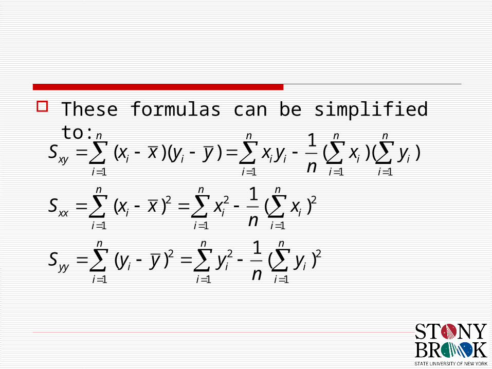
These formulas can be simplified to:

1 1 1 1

2 2 2

1 1 1

2 2 2

1 1 1

1( )( ) ( )( )

1( ) ( )

1( ) ( )

n n n n

xy i i i i i ii i i i

n n n

xx i i ii i i

n n n

yy i i ii i i

S x x y y x y x yn

S x x x xn

S y y y yn

gives the sum of cross-products of the x’s

and Y’s around their respective means.

and give the sums of squares of the

differences between the and , and the and , respectively.

These expressions can be simplified to:

xyS

xxS yySix

iy iy

0 1 1xy

xx

Sy x

S

ix

The least squares (LS) line, which is an estimate of the true regression line is:

0 1ˆ ˆy x

Find the equation of the line for the number of sales due to increased advertising

and n=5 which allows us to get

2 2247 , 98 , 13327 , 2038 , 5192i i i i i ix y x y x y

49.4 ; 19.6x y

1 1 1

15

1( )( ) 350.80247 98

n n n

xy i i i i

i i i

S x y x yn

2 2 2

1 1

15

1( ) 13327 (247) 1125.20

n n

xx i i

i i

S x xn

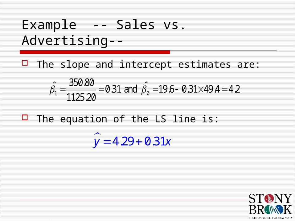
The slope and intercept estimates are:

The equation of the LS line is:

1 0

350.80ˆ ˆ0.31 and 19.6 0.31 49.4 4.21125.20

4.29 0.31y x


Coefficient of Determination and Coefficient of Correlation

Residuals are used to evaluate the goodness of fit of the LS line:

0 1ˆ 1,2,.....i iy x i n

0 1ˆ ˆ( ), 1,2,.....i i ie y x i n

2min iQ e

Error sum of squares (SSE):

Qmin also equals:

This is the total sum of squares (SST).

2min iQ e

22

2 1

1 1 1

n n n

ii i yyni i i

y y y y S

Total Sum of Squares:

Regression Sum of Squares:

, where

is the ratio.

2 2 2

1 1 1 1

0

ˆ ˆ ˆ ˆ( ) ( ) ( ) 2 ( )( )n n n n

i i i i i i ii i i i

SSR SSE

SST y y y y y y y y y y

SST SSR SSE 2 1

SSR SSEr

SST SST

Sales vs. AdvertisingCoefficient of Determination and Correlation

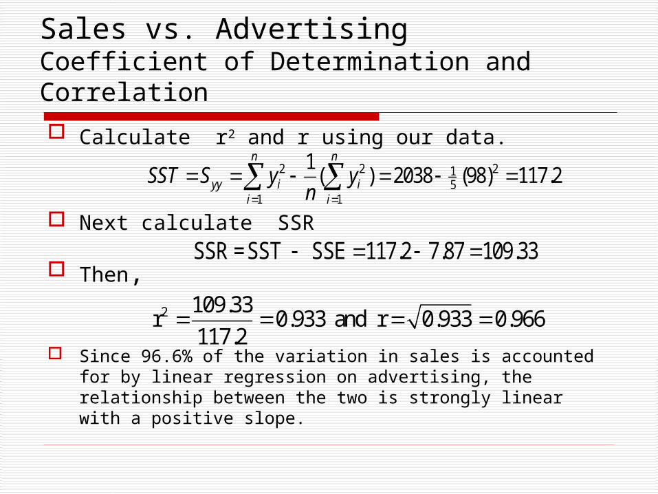
Calculate r2 and r using our data.

Next calculate SSR

Then,

Since 96.6% of the variation in sales is accounted for by linear regression on advertising, the relationship between the two is strongly linear with a positive slope.

2 2 215

1 1

1( ) 2038 (98) 117.2

n n

yy i ii i

SST S y yn

SSR =SST SSE 117.2 7.87 109.33

2 109.33r 0.933 and r 0.933 0.966

117.2

Estimation of 2

Variance 2 measures the scatter of the around their means.

The unbiased estimate of the variance is given by:

iY

2

2 1

2 2

n

ii

eSSE

sn n

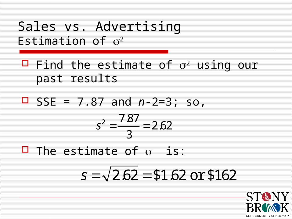
Find the estimate of 2 using our past results

SSE = 7.87 and n-2=3; so,

The estimate of is:

2 7.872.62

3s

2.62 $1.62 or $162s

Sales vs. AdvertisingEstimation of 2

Statistical Inference on and

ⅰ. Point Estimator

ⅱ. Confidence Interval

ⅲ. Test

Distributions of and

Point estimators

100(1 -)% IC

2

0( ) i

xx

xSE s

nS

xxS

N2

11 ,~ˆ

xx

i

nS

xN

22

00 ,~ˆ

1( )xx

sSE

S

0

1

2 20 0 1 12, 2,

,n nt SE t SE

Hypothesis test

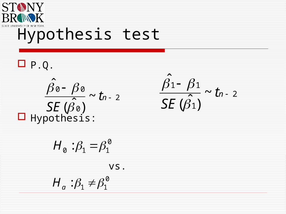
P.Q.

Hypothesis:

vs.

2

0

00~

)ˆ(

ˆ

nt

SE

2

1

11~

)ˆ(

ˆ

nt

SE

00 1 1:H

01 1:aH

Test Statistics:

Reject region: reject Ho at if:

01 1

0

1( )t

SE

1

0

1( )t

SE

0 2, / 2nt t

Analysis of Variancefor Simple Linear Regression

The analysis of variance (ANOVA) is a statistical technique to decompose the total variability in the yi’s into separate variance components associated with specific sources.

Mean square is a sum of squares divided by its d.f.

Mean Square Regression

Mean Square Error

SSRMSR=

1

SSEMSE=

2n

The ratio of MSR to MSE provides an equivalent to test the significance of the linear relationship between x and y:

2 22 01 1 2

1, 22 2

1

ˆ ˆ ˆ1~

ˆ/ ( )

xxn

xx

HMSR SSR St F

MSE s s s S SE

ANOVA table

Source of Variation

(Source)

Sum of Squares

(SS)

Degrees of Freedom

(d.f.)

Mean Square

(MS)

F

Regression

Error

SSR

SSE

1

n – 2

Total SST n - 1

1

SSRMSR

2

SSEMSE

n

MSRF

MSE

Prediction of Future observations

Suppose we fix x at specified value x*

How do we predict the value of the r.v. Y*?

Point Estimator:

* **

0 1Y x

Prediction Intervals (PI) The Confidence Intervals for Y* and E(Y*) are

called Prediction Intervals.

Formulas for a 100(1-α)% PI:

2 2

1 12, /2 2, /2

2 2

1 12, /2 2, /2

* ** * *

* ** 1 * * 1

n nn nXX XX

n nn nXX XX

x x x xt s t s

S S

x x x xY t s Y Y t s

S S

s MSE

Cautions about making predictions

Note that the PI will be shortest when x* is equal to the sample mean.

The farther away x* is from the sample mean the longer the PI will be.

Extrapolation beyond the range of the data is highly imprecise and should be avoided.

Example 10.8 Calculate a 95% PI for the mean groove depth of the

population of all tires and for the groove depth of a single tire with a mileage of 25,000 (based on the date from earlier sections).

In previous examples, we already measured the following quantities:

*0 1

7,0.025

25 * 178.62

19.02 ; 960

16 ; 9 ; 2.365

XX

x x

s S

x n t

Example 10.8 (continued) Now we simply plug these numbers into our

formulas

95% PI for E(Y*):

95% PI for Y*:

219

(25 16)178.62 2.365 19.02 [158.73,198.51]

960

219

(25 16)178.62 2.365 19.02 1 [129.44,227.80]

960

Calibration (Inverse Regression)

Suppose we are given μ*=E(Y*), and we want an estimate of x*.

We simply solve the linear regression formula for x* to obtain our point estimator:

Calculating the CI is more complicated and is not covered in this course.

0

1

**x

Example 10.9 Estimate the mean life of a tire at wearout

(62.5 mils remaining). We want to estimate x* when μ*=62.5 From previous examples, we have calculated:

Plugging this data into our equation we get:

0

1

360.64

7.281

62.5 360.64* 1000 40,947.67

7.281x

REGRESION DIAGNOSTIC

The four basic assumptions of linear regression need to be verified from data to assure that the analysis is valid.

1. The mean of is a linear function of

2. The have a common variance ,which is

the same for all values of

3. The errors are normally distributed.

4. The errors are independent.

iYix

2iY

x

ii

Checking The Model Assumptions

If the model is correct, then the residuals

can be viewed as the “estimates” of the random errors ‘s.

Residual plots are the primary tool.

iii yye ˆi

Checking for Linearity Checking for Constant Variance Checking for Normality Checking for Independence

How to do this?

If regression of y on x is linear, then the plot of ei vs. xi

should exhibit random scatter around zero.

Checking for linearity

Example 10.10

1 0 394.33 360.64 33.69

2 4 329.50 331.51 -2.01

3 8 291.00 302.39 -11.39

4 12 255.17 273.27 -18.10

5 16 229.33 244.15 -14.82

6 20 204.83 215.02 -10.19

7 24 179.00 185.90 -6.90

8 28 163.83 156.78 7.05

9 32 150.33 127.66 22.67

i ix iy iy ie

The plot is clearly parabolic. The linear regression does not fit the data adequately. Maybe we can try a second degree model:

2210 xxy

Plot vs. .

Since the are linear functions of , we can also plot vs. .

If the constant variance assumption is correct,

ie iy

iy ix ie ix

The plot of

vs.

would be like

2)( ieVar

ie iy

Checking for Constant Variance

Checking for normality

Making a normal plot1. The normal plot requires that the observations form a random sample

with a common mean and variance.

2. The do not form such a random sample, depend on

and hence are not equal.

3. Residuals using to make normal plot (They have a zero mean and an

approximately constant variance.

iy iiYE )( ix

Example 10.10

Checking for normality

A well-known statistical test is the Durbin-Watson Test

n

uu

n

uuu

e

eed

1

2

2

21)(

1. When d is more near 2, residuals are more independent.

2. When d is more near 0, residuals are more positively

correlated.3. When d is more near 4, residuals are more negatively

correlated.

Checking for Independence

CHECKING FOR OUTLIERS AND INFLUENTIAL OBSERVATIONS

Checking for Outliers

*

2, 1, 2,..., .

( ) ( - )11

i i ii

i i

xx

e e ee i n

SE e sx xs

n S

*If 2, then the corresponding observation may be regarded an outlier.ie

Standard residuals

Checking for Influential Observations

An influential observation is not necessarily an outlier. An observation can be influential because it has an extreme

x-value, an extreme y-value, or both. How can we identify influential observations?

Leverage

1 1

ˆ , 1n n

i ij j iij i

y h y h k

A rule of thumb is to regard any 2( 1) / as high leverage.

The observation with high leverage is an .

In this chapter, 1, and so

influential observati

4 / is regar

o

d

n

ed as high leverage.

The fo

ii

ii

h k n

k h n

2( )1

rmula for for 1 is given by iii ii

xx

x xh k h

n S

ˆ can be expressed as a linear combination of all the as follows:i jy y

where the are some functions of the 's. We call as the .leverageij ijh x h

How to Deal with Outliers and Influential Observations?

Two separate analyses may be done, one with and one without the outliers and influential observations.

Example 10.12

No.

1 2 3 4 5 6 7 8 9 10 11

X 8 8 8 8 8 8 8 19 8 8 8

Y 6.28 5.76 7.71 8.84 8.47 7.04 5.25 12.50 5.56 7.91 6.89

ei* -0.341 -1.067 0.582 1.735 1.300 0.031 -1.624 0 -1.271 0.757 -0.089

hii 0.1 0.1 0.1 0.1 0.1 0.1 0.1 1 0.1 0.1 0.1

DATA TRANSFORMATIONS

Linearizing Transformations Simple Functional relationship

i.e power form: y x

ln ln

ln ln

y x

x

ln and lny y x x then

produce

0 1ln and


Linearizing Transformations Simple Functional relationship

i.e exponential form:

then

produce

xy eln ln

ln

xy e

x

ln andy y x x

0 1ln and

2

3

1

log

y

x y

x y

x y

x y

x

21

3

log

x

x y

x y

y

x y

x y

21

3

log

x

x y

x y

y

x y

x y

2

3

2

3

x y

x y

x y

x y

x yx

y


Linearizing Transformations

Linearizing Transformations Ex. 10.13 (Tire tread wear vs. Mileage: Exponential Model)


x

y

Linearizing Transformations Ex. 10.13 (Tire tread wear vs. Mileage: Exponential Model)


y

x


Variance Stabilizing Transformations Based on two-term Taylor-series approximations Given relationship between mean and variance:

The following transformation makes variances approximately equal, even if means differ :

2( )

12( ) ( )( ) u uY f x f


Variance Stabilizing Transformations Delta Method

Let:

then

consequently

22 2 ( )

( ) ( ) ( )Var

VarE

YY g

h h gY

2 2( ) ( ) ( )

( )

11h g h

g

( )( )

dgh

( )( )

y

dygyh

DATA TRANSFORMATIONS Variance Stabilizing Transformation

Example 1

here

then

2 2Var 0Y c c

( )g c

1 1

( )

ln

dycy

dyc y c

yh

y

2Var 0Y c c

Example 2

here

then

( )g c

1 2

( )dy

c y

dyc cy

yh

y

CORRELATION ANALYSISBackground on correlation

A number of different correlation coefficients are used for different situations. The best known is the Pearson product-moment correlation coefficient, which is obtained by dividing the covariance of the two variables by the product of their standard deviations. Despite its name, it was first introduced by Francis Galton.

CORRELATION ANALYSIS

•When it is not clear which is the predictor variable and which is the response variable?

•When both variables are random?

Bivariate Normal Distribution

Correlation: a measurement of how closely two variables share a linear relationship. Or the measure of independence.

If =0 , uncorrelated, that implies independence, but does not guarantee it

If =-1 or +1, it represents perfect association

Useful when it is not possible to determine which variable is the predictor and which is the response. Health vs Wealth. Which is predictor? Which is response?

Y)Var(X)Var(

Y) Cov(X, Y) corr(X,

p.d.f. of (X,Y)

Properties p.d.f is defined at -1<<1 Undefined if =±1 and is called degenerate. The marginal p.d.f of x is

The marginal p.d.f of Y is

2( , )X XN


2 2

2

12

2(1 )

2

1( , )

2 1

X X Y Y

X X Y Y

x x y y

X Y

f x y e

2( , )Y YN

How to calculate Let

f(X,Y) has a covariance =

where

2 2( ) ( , ) ; ( ) ( , )X X Y Yf x N f Y N

2

2 2 2 2 2 2 2 2

2det 1X X Y

X Y X Y X Y

X Y Y

2

2X X Y

X Y Y

A

Calculation

wwhere N=2 since it is bivariate bi=2, thus:

wwhere

2 1

2

21( , )

2 det

X Y

N

x y A

f X Y eA

2 1

2

2

2 2 2

1( , )

2 1

X Y

N

x y A

X Y

f X Y e

2

1

22 2 2

1

1Y X Y

X Y XX Y

A

Calculation (cont…)

2 22 2

2 2 2

21

2(1 )

2

1( , )

2 1

Y X X Y X Y X Y

X Y

x y x y

X Y

f x y e

2 2

2 2 2

21

2(1 )

2

1( , )

2 1

X X Y Y

X YX Y

x x y y

X Y

f x y e

Statistical Inference on the Correlation Coefficient ρ

We can derive a test on the correlation coefficient in the same way that we have been doing in class. Assumptions

X, Y are from the bivariate normal distribution Start with point estimator

R: sample estimate of the population correlation coefficient ρ

Get the pivotal quantity The distribution of R is quite complicated T: transform the point estimator into a p.q.

Do we know everything about the p.q.? Yes: T ~ tn-2 under H0 : ρ=0

n

ii

n

ii

i

n

ii

YYXX

YYXXR

1

22

1

1

)()(

))((

21

2

R

nRT

Derivation of T

Therefore, we can use t as a statistic for testing against the null hypothesis

H0: β1=0

Equivalently, we can test against

H0: ρ=0

1

21

1 1 1

22

1 11 2

1

are these equivalent?

ˆ?2ˆ( )1

substitute:

ˆ ˆ ˆ

( 2)1

then:

ˆ ˆ( 2)ˆt yes, they are equivalent.ˆ( 2) ( )

xx

x xx xx

y yy

xx

sS

r nt

SEr

s S Sr

s S SST

SSE n sr

SST SST

S n SST

SST n s SE

Exact Statistical Inference on ρ Test H0 : ρ=0 vs. Ha : ρ≠0

Test Statistics

22

2

1n

r nt t

r

0 1 1: 0 . : 0aH vs H

1 1 1

22

11 222

ˆ ˆ ˆ

( 2)1

ˆ2 ˆ ( 2)( 2)1

x xx xx

y yy

xxn

xx

S S Sr

S S SST

n sr

SST

Sr n SSTt n t

SST n s s Sr

( ) YY X

X

Y

X

E Y x x

Exact Statistical Inference on ρ (Cont.)

Reject Region : Reject H0 if t0 > tn-2

Example: The times for 25 soft drink deliveries (y) monitored as a function of

delivery volume (x) is shown in table next page. Testing the null hypothesis that the correlation coefficient is equal to 0.

Data

Y X Y X Y X Y X Y X

7 16.68 7 18.11 16 40.33 10 29.00 10 17.90

3 11.50 2 8.00 10 21.00 6 15.35 26 52.32

3 12.03 7 17.83 4 13.50 7 19.00 9 18.75

4 14.88 30 79.24 6 19.75 3 9.50 8 19.83

6 13.75 5 21.50 9 24.00 17 35.10 4 10.75

Exact Statistical Inference on ρ

Solution The sample correlation coefficient is

for α = .01,

Reject H0

1

2 2

1 1

( )( )2473.34

0.961136.57 * 5784.54

( ) ( )

n

i i

i

n n

i i

i i

X X Y Y

R

X X Y Y

02 2

2 0.96 * 25 217.56

1 1 0.96

r nt

r

0 23,0.00517.56 2.807t t

Exact Statistical Inference on ρ

Approximate Statistical Inference on ρ

There is no exact method of testing ρ vs an arbitrary ρ0 Distribution of R is very complicated T ~ tn-2 only when ρ = 0

To test ρ vs an arbitrary ρ0 use Fisher’s Normal approximation

Transform the sample estimate

1 1 12 2

1 1 1tanh ln ln ,

1 1 3

RR N

R n

01 102 2

0

11 1ln , under H , ~ ln ,

1 1 3

rN

r n

Sample estimater:

CI:


Test :

Z statistic:

12

1ln

1

r

r

0 03z n

0 0 1 0

010 0 1 02

0

: vs. :

1: ln vs. :

1

H H

H H

/2 /2

2 2

2 2

1 1

3 3

1 1

1 1

l u

l u

z zn n

e e

e e

reject H0 if |z0| > zα/2

Code:


Output:


Retaking the previous example: The times for 25 soft drink deliveries (y) monitored as a function of

delivery volume (x) is shown in table next page. Testing the null hypothesis that the correlation coefficient is equal to 0.


SAS coding for last exampledata corr_bev;input y x;datalines;7 16.683 11.53 12.034 14.886 13.757 18.112 8.007 17.8330 79.245 21.516 40.3310 21.004 13.56 19.759 24.0010 29.006 15.357 19.003 9.5017 35.110 17.9026 52.329 18.758 19.834 10.75;run;proc gplot data=corr_bev;plot y*x;run;proc corr data=corr_bev outp=corr;var x y;run;

SAS analysis for last example

Pitfalls of Regression and Correlation Analysis

Correlation and causation Good mood cause good health

Coincidental data Baldness and lawyers

Lurking variables(third unobserved variable) Relationship between eating and weight, with

unobserved variable of heredity(metabolism,and illness).

Restricted range IQ, school performance (elementary school to

college) college lower IQ’s are less common so there would clearly be a decrease in the range.

Correlation and linearity The correlation value may not

be enough to evaluate a relationship, especially in the case where the assumption of normality is incorrect.

This image created by Francis Anscombe, has common mean (7.5), standard deviation(4.12), correlation (.81) and regression line y=3+.5x

Pitfalls of Regression and Correlation Analysis

SIMPLE LINEAR REGRESSION AND CORRELATION

Prepared by:Jackie ZerleDavid FriedChun-Hui ChungWeilai ZhouShiyhan ZhangAlex FieldsYu-Hsun ChengRoosevelt Moreno

AMS 572.1 DATA ANALYSIS, FALL 2007.

SIMPLE LINEAR REGRESSION AND CORRELATION Prepared by: Jackie Zerrle David Fried Chun-Hui Chung...

Documents

Transcript of SIMPLE LINEAR REGRESSION AND CORRELATION Prepared by: Jackie Zerrle David Fried Chun-Hui Chung...