The Simple Fool’s Guide to Population Genomics via RNA­Seq: An Introduction to High­Throughput Sequencing Data Analysis 

  

* 

Me ,2+ Pierre De Wit 1+

1lissa H. Pespeni  Jason T. Ladner 1

Daniel J. Barshis 1 François Seneca 1 

Nina Overgaard Therkildsen 3 Hannah Jaris 1 

Megan Morikawa 4 Stephen R. Palumbi 1 

  

1. w Department of Biology, Stanford University, Hopkins Marine Station, 120 Ocean vieBlvd., Pacific Grove, CA 93950, USA. 

2. Department of Biology, Indiana University, 915 E. Third Street, Myers Hall 150, Bloomington, IN 47405‐7107, USA. 

3. National Institute of   Denmark, Vejlsøvej Aquatic Resources, Technical University of. 39, 8600 Silkeborg, Denmark

4. Duke University, Durham, NC 27708, USA. + equally contributing authors 

* corresponding author: pdewit@stanford.edu 

The Simple Fool’s Guide to Population Genomics via RNA­Seq: An Introduction to High­Throughput Sequencing Data Analysis  List of contents 

Introduction (p.3)  

 A  –  rocessing samples   Section 0 ‐ Preparing cDNA libraries for high‐throughput short‐read sequencing (p.6) ct I P

 rmission Setting up your computer (p.9) 

I nte

  – Preparing for data analysis 

ess g of RNA‐Seq data (p.20) Act II  Section 1 – Quality control proc in

    Section 2 – De novo assembly (p.26)

(p.2     Section 3 – BLAST and annotation  9)

 Section 4 – Mapping to reference (p.36) 

   

 – Data analysis  a

Act III  Section 5 – Gene expression and functional enrichment nalyses (p.40)    Section 6 – SNP detection, principal components and FST outlier analyses (p.45)

2

Introduction This document is intended as a guide to help researchers dealing with non‐model organisms acquire and process high‐throughput sequencing data without having to acquire extensive bioinformatics skills. The guide covers the process from tissue collection, sample preparation and computer setup, to addressing biological questions with gene expression and SNP data. A user who is thinking about starting a new project might want to read through this document before deciding on the best sampling scheme. A user who already has sequence data can instead pickup at an appropriate step within the guide, depending on the specifics of the project. By walking through this protocol with the provided scripts and sample files, the user will gain a basic understanding of the bioinformatic work involved in high‐throughput sequence data analysis, while avoiding having to learn computer programming skills. In the long run, any researcher who wants to create a custom analysis will have to acquire certain programming skills, but by focusing on learning the general principles of bioinformatics first, this protocol provides a starting point for further learning. 

While the focus is on high‐throughput sequence data generated from mRNA, in modified form this protocol can also be relevant to data from other types of sequence data, such as whole genomic DNA or RAD‐Tags. The protocol can also be used for organisms for which the  re are genomes or transcriptomes available. In those cases, several of the steps (de novoassembly and annotation) can be omitted.  

All instructions are written for Mac OS X, but will also work (with slight modifications) on a Linux machine or on a PC running a Unix emulator. 

RNA‐Seq is a general term to describe the process of high‐throughput sequencing of all messenger RNA (the ”transcriptome”) present in a specific tissue type. High‐throughput sequencing typically generates millions of short reads for each sampled individual. Combining all of these short reads into mRNA transcripts, then using the transcripts to detect genetic variation, however, is not a trivial task and requires considerable computing power and knowledge of computer programming. With the increasing power of desktop computers, it is now possible to assemble and analyze entire transcriptomes at home, yet many biologists lack the computer know‐how to process these immense datasets. This protocol aims at guiding someone who has little to no background knowledge in computer programming through an analysis of RNA‐Seq data. The guide is intended to be an example of one way to process this kind of data in order to address a few specific biological questions (outlined below). This is by no means an exhaustive protocol, and there are many other ways to process and analyze RNA‐Seq data. However, we feel the methods outlined her tom ein provide an approachable, functional platform from which to build your own cusanalysis. 

An advantage of RNA‐Seq is the ability to collect both gene expression and genetic polymorphism (single nucleotide polymorphisms or SNPs) data from a single data set. By comparing control and treatment datasets, differential gene expression can identify genes that are being up‐ or downregulated in response to a particular experimental treatment. Further, by grouping genes by gene ontology (GO) functional categories, we can gain knowledge of exactly what groups of molecular processes are being affected by a prescribed change in an organism’s environment. SNP data are commonly used for identifying genetic structure within geographical areas, either by calculating metrics such as FST (the proportion of genetic diversity due to allele frequency differences among populations) or 

3

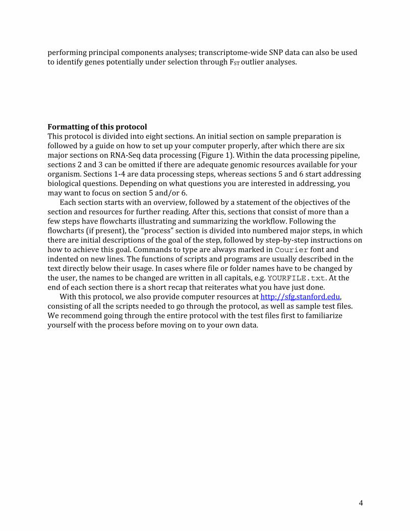
performing principal components analyses; transcriptome‐wide SNP data can also be used to identify genes potentially under selection through FST outlier analyses.  Formatting of this protocol This protocol is divided into eight sections. An initial section on sample preparation is followed by a guide on how to set up your computer properly, after which there are six major sections on RNA‐Seq data processing (Figure 1). Within the data processing pipeline, sections 2 and 3 can be omitted if there are adequate genomic resources available for your organism. Sections 1‐4 are data processing steps, whereas sections 5 and 6 start addressing biological questions. Depending on what questions you are interested in addressing, you may want to focus on section 5 and/or 6. 

Each section starts with an overview, followed by a statement of the objectives of the section and resources for further reading. After this, sections that consist of more than a few steps have flowcharts illustrating and summarizing the workflow. Following the flowcharts (if present), the “process” section is divided into numbered major steps, in which there are initial descriptions of the goal of the step, followed by step‐by‐step instructions on how to achieve this goal. Commands to type are always marked in Courier font and indented on new lines. The functions of scripts and programs are usually described in the text directly below their usage. In cases where file or folder names have to be changed by the e  user, the names to be changed are written in all capitals, e.g. YOURFILE.txt. At thend of each section there is a short recap that reiterates what you have just done. 

With this protocol, we also provide computer resources at http://sfg.stanford.edu, consisting of all the scripts needed to go through the protocol, as well as sample test files. We recommend going through the entire protocol with the test files first to familiarize yourself with the process before moving on to your own data. 

4

1. Quality Control processing of raw data

5c. Functional enrichment analyses

2. de novo assembly 3. Annotation

4. Map reads to reference

6a. Alignment processing 5a. Expression count

5b. Expression normalization and test for differences

6b. Variant detection, annotation and filtration

6c. Genotype extraction and analysis

Figure 1. Overview of RNA-Seq data processing, as described in this protocol.

5

0. Fresh tissue to cDNA Libraries  Overview The first step in RNA‐Seq sample preparation is to choose a tissue from which you will extract total RNA. Following total RNA extraction you will purify mRNA that will be used as templates to synthesize complementary DNA, also known as cDNA. These resulting cDNA libraries will be used for sequencing. 

When selecting the tissue it is important to be consistent in your sampling of different individuals/treatments/locations. Keep in mind that gene expression and SNP detection will be affected by both environmental conditions and tissue type. Before starting the lab work, it is important to note that RNA is highly susceptible to degradation by RNAse enzymes. These enzymes can be found in the air and on your clothing and hands. It is very important to utilize good laboratory practices and work as efficiently as possible through cDNA synthesis. Once you have double stranded cDNA you can breathe a little easier, because cDNA is more stable than RNA. While there are many RNA extraction kits to choose from we recommend using Qiagen’s RNeasy extraction kit. It is a very fast and easy procedure, free from toxic chemicals. However, if you plan to also extract genomic DNA from your tissue, a Trizol extraction method may be preferable. While there are also many cDNA library preparation kits, Illumina’s TruSeq RNA sample preparation kit is all‐inclusive. It includes all the necessary reagents to purify mRNA from total RNA and make cDNA libraries. The protocol is straightforward and there is peace of mind knowing the manual was written and tested by the manufacturers of the Illumina sequencing machine. 

Unless you have direct access to a next‐generation sequencing machine, you will need to send your generated cDNA libraries off for sequencing. There are a number of sequencing centers that would be happy to sequence your samples. When selecting a sequencing facility, there are, however, some important things to consider. 1) Whether or not the center performs a quantification step using qPCR and/or an Agilent Bioanalyser (Illumina recommends qPCR). Some centers require this to be done prior to sample submission. 2) Whether or not the center can pool barcoded samples for you or if you have to do that prior to sample submission. 

nths, depending on their 3) How long sequencing takes (ranges from 10 days to several moworkload). 4) How responsive their customer support is via e‐mail or phone. 5) Cost. Some sequencing facilities will also do the sample preparation for you. It is up to you to weigh the options of cost vs. work. 

To ensure high quality sequence data, it is usually safer to pick a sequencing center that uses both qPCR and the Agilent Bionalayzer for quality control of cDNA libraries. It may be mportant to the user that the sequencing takes place in a timely fashion, and it is extremely elpful if the facility’s customer support is responsive. ih Objectives The objectives for this section are to 1) extract total RNA from fresh, frozen, or RNAlater‐ preserved tissue samples, 2) purify and fragment mRNA from total RNA and, 3) create cDNA libraries from mRNA that will be sent off for sequencing. 

6

Resources Gayral P, Weinert L, Chiari Y, Tsagkogeorga G, Ballenghien M, Galtier N. 2011. Next‐generation sequencing of transcriptomes: a guide to RNA isolation in nonmodel animals. Molecular Ecology Resources 11: 650‐661.  Collins L, Biggs P, Voelckel, C, Joly, S. 2008. An approach to transcriptome analysis of non‐model organisms using short‐read sequences. Genome Informatics 21: 3‐14.  Mortazavi A, Williams BA, McCue K, Schaeffer L, Wold B. 2008. Mapping and quantifying mammalian transcriptomes by RNA‐Seq. Nature Methods. 5: 621‐628.   RNA extractio nd protocn kits a ols http://www.qiagen.com/hb/rneasymini  Quantification/validation of samples http://www.invitrogen.com/site/us/en/home/brands/Product‐Brand/Qubit.html  Library Prep/RNA seq technology 

products/datasheets/datasheet_TruSeq_sample_prhttp://www.illumina.com/documents//ep_kits.pdf http://www.illumina.com/TruSeq.ilmn  Other high‐throughput sequencing technologies and systems include:  Applied Biosystems SOLiD 

en/home/applications‐(http://www.appliedbiosystems.com/absite/us/technologies/solid‐next‐generation‐sequencing.html) Roche 454 Life Science (http://www.454.com/) Helicos Biosciences tSMS (http://www.helicosbio.com/Technology/TrueSingleMoleculeSequencing/tabid/64/Default.aspx).  Process 1. U  Qse iagen’s RNeasy Kit (www.qiagen.com/hb/rneasymini) to extract total RNA from 

your tissue. a. A tissue‐lyser is a great way to disrupt the tissue sample. 

2. Q antt

u tify the amount of total RNA in each sample using a QuBit RNA assay. (h p://products.invitrogen.com/ivgn/product/Q32852). a. You will want to standardize across samples the amount of total RNA you use to sta

  library preparation. 1 µg of total RNA is often a good amount to start with.  t ‐80°C until 

rt  

3. Flash‐freeze the freshly extracted total RNA in liquid nitrogen and place aready to proceed with library preparation. 

. Prepare libraries following the Illumina TruSeq Preparation Kit protocol (

4www.illumina.com/.../datasheet_TruSeq_sample_prep_kits.pdf) 

   

7

Summary You have now extracted total RNA from a tissue, purified mRNA from the total RNA, and from this mRNA have created cDNA libraries that are ready for sequencing. Congratulations! You are well on your way to collecting a single data set that contains both gene expression and SNP data from the tissue you have selected.

8

 How to set up your computer to run smoothly through this protocol  Overview Stop! Do not go any further before you have set up your computer. This will allow you to move through the pipeline without stuttering the whole way trying to install programs, packages and dependencies. It may take a day, but just commit yourself to it! In this text, we are walking through the installation process on a new Mac with an Intel processor and the Lion (OS X version 10.7) or Snow Leopard (OS X version 10.6) operating system. This does not mean that a Mac is required, but Mac OS X is currently one of the most ommonly used operating systems for bioinformatics, along with various versions of the inux operating system family.  cL 

A note on operating systems Mac OS X and Linux are both rooted in an operating system called “UNIX”, which has a long‐standing tradition of open source. This means that many software packages can be complied on Mac OS X, Linux, and BSD systems alike. Linux can be a very useful operating system, as it is free in most of its versions, and works on both Macs and PC’s. It can nevertheless be perceived as having a steep learning curve. We have used Ubuntu Linux in our lab, as it is easy to install and use both on a PC running Windows and on a Mac. With minor modifications (see Appendix 1 of Haddock and Dunn (2010) for useful tips), it is possible to run this pipeline on a Windows PC (without installing Linux). This requires that a “UNIX environment portal” is installed. We have tried Cygwin, which we found to work well. The present protocol, however, assumes that the reader is using a relatively new Mac with an Intel processor and Mac OS X “Lion” or “Snow Leopard” installed. 

 There is often more than one way of installing a program on your computer. On Macs, 

the simplest is usually to download an installer .dmg package, which installs itself when you click on it. Sometimes, however, that is not available, making it necessary to download executable files and copy them manually to your hard drive. In some cases, you might even have to download the source code for programs and build them on your computer, for which you’ll need special compiler software. The advantage of compiling your own software is that the software will be “custom‐built” for your computer setup, and will run more smo d othly than a version compiled somewhere else might. A list of all the software discussein this chapter, along with information on where to find it, can be found in Table 1. 

Before getting started with the process below, we highly recommend reading through chapters 4, 5, and 6 from Haddock and Dunn’s (2011) “Practical Computing for Biologists” to gain comfort and familiarity with how UNIX‐based operating systems such as Mac OS X and Linux are organized and how they process information. This reading will also make you comfortable with working through the command line in the Terminal window environment, which is essential to most of this protocol. Terminal is an application that allows you to interact with your computer through the command line. Using the command line, you can navigate around your computer as you do in Finder. You can open and manage files and folders and execute programs. The default shell, the program that displays the command 

9

line   (the prompt and cursor), in Mac OS X is called “bash”. A short summary of some of themost useful bash commands can be found at the end of this section. 

When naming files and folders, there are a few simplifying rules to follow. Spaces and special characters are to be avoided. Also, you want make file names as informative as possible in a filename without making them too long, so abbreviations are nice. If you are planning to run through the protocol several times, it is helpful to add date and time to a filename (do not just call the file “new”). If you are planning to share files, adding your initials at the end can also be useful. It is also important to note that many of the files gen ‐erated in this protocol are huge. It is important to make sure that there is enough harddrive space before starting. 

Throughout this protocol, we refer to “bash scripts”, “scripts” and “programs”. A bash script consists of a list of commands that you could just as well type directly into the Terminal. The advantage of using a bash script is that it facilitates the “batch” processing of many different files at the same time, since you can execute a series of commands one right after another, without having to enter each one manually. A bash script normally starts with #!/bin/bash and the filename extension is .sh. The bash scripts used in this protocol were written by us, and in general you will have to open them in a text editor and modify input and output file names. “Scripts” are programs that we have written in an interpreted (non‐compiled) high‐level programming language, such as Perl (.pl), Python (.py) or R (.r). You will not need to open the scripts used in this protocol unless you want to study exactly how they work or modify them in some form. Within most bash scripts and scripts there are lines that begin with #; these are comment lines for your benefit and are not used by the computer. Reading these lines will help you understand what the script does. “Programs”, as used herein, refers to executable files that have been precompiled to binary code, and thus cannot be opened in a text editor in any meaningful way. The programs used here wer uire e not written by us, nor should you try to change any of their contents; how to acqthem is the focus of the rest of this section.  

The scripts provided in the “scripts” repository (http://sfg.stanford.edu) are free software: you can redistribute them and/or modify them under the terms of the GNU General Public License as published by the Free Software Foundation, version 3 of the License. These programs are distributed in the hope that they will be useful, but WITHOUT ANY WARRANTY; without even the implied warranty of MERCHANTABILITY or FITNESS FOR A PARTICULAR PURPOSE. See the GNU General Public License for more details. You sho grams uld have received a copy of the GNU General Public License along with these pro(gpl.txt). If not, see http://www.gnu.org/licenses/. 

Below, you will find one way to setup your Mac computer. If you have problems installing any of the software, you can also try using a package manager such as MacPorts (http://www.macports.org/) or Fink (http://www.finkproject.org/).  Objectives 1) Set up your computer so that it understands where to find the programs and scripts (PATH), and how to interpret the programming languages that we use in this pipeline. ) Install the software that we will use generally and within the different sections of the rotocol. 2p  

10

  Resources 

 and Dunn (2011). Practical Computing for Biologists. Sinauer Associates, Inc. un , MA, USA. HaddockderlandTable 1 

S

 Process 

Par 1t   – Basic setup: PATH, compilers, programming languages and modules 

1. Create a “scripts” and a “programs” folder in your home directory. 2. Set up PATH. This will tell your computer where to look for programs and files. From 

your home directory (see instruc s for how to move betwee  directories at the end of this section) in Terminal,  : 

tion ntype

nano .bash_profile (or edit .bash_profile)  This will create a file if it doesn’t exist already. Type in the file: PATH=”~/scripts:~/programs:${PATH}”

export PATH Now, save and exit the file.

3. Download the Xcode package from the AppStore and install. If installing XCode 3, 

make sure to include the optional 10.4 SDK tools which are needed for Biopython below. 

4. Download and install gcc (Fortran compiler) from http://hpc.sourceforge.net/ (we downloaded gcc‐lion.tar.gz).  In Terminal, move into the “downloads” directory and if your computer has not automatically unzipped the file and removed the “.gz” file extension, type:  

gunzip gcc-lion.tar.gzThen, to install the compiler into the /usr/local folder (where your computer will be able to find it), type: 

sudo tar –xvf gcc-lion.tar –C / The “sudo” command overrides your computer’s default security settings in order to write to a folder outside of your home directory. You will need administrator access (and password) in order to do this. Also download the g77 compiler (g77-intel-bin.tar.gz). From the “downloads” folder in Terminal, type (as above):

gunzip g77-intel-bin.tar.gz sudo tar –xvf g77-intel-bin.tar –C /

Once the process is finished, you can delete the downloaded installation files. 5. Download and install Git from 

http://git‐scm.com/download.  This is a program for 

downloading other programs from within Terminal (Git v1.7.6 built for rsion if working on a SnowLeopard seems to work with Lion. Choose the x86_64 ve

64‐bit Intel Mac). 6. Check that Python is installed. Open a Terminal window, type: 

python The first line should print the version (we’re using version 2.7.1). 

7. Make sure that numpy is installed. In the python interpreter in Terminal (you should be there if you typed python in point 6), type: 

import numpy

11

If it is installed you should just get a new line, if not you will get an error. It should already be installed if you’re working with python version 2.7. If you’re working with an older version you install numpy using Git (or download it with a web browser, the link is given in Table 1). Open a new Terminal window or quit python with quit() (so that you’re no longer in the python interpreter) and move into your programs folder. Then type: 

git clone git://github.com/numpy/numpy.git numpy Then move into the new numpy folder and type:

sudo python setup.py install 8. Install scipy: From your programs folder, type: 

git clone git://github.com/scipy/scipy.git scipy Then move into the new scipy folder, type:

sudo python setup.py install 9. Download the latest version of Biopython (we’re installing the biopython‐1.57 source 

tarball) and unzip it by double‐clicking on the file in a finder window. Then, in the Terminal, move into the biopython folder that you unzipped and type: 

python setup.py build python setup.py test sudo python setup.py install

Once these packages (numpy, scipy and biopython) are installeddownloaded installation files.

10. Check that Perl is installed. Open a Terminal window, type: 

you can delete the

perl –version The first line should print the version (we’re using version 5.12.3). Perl should be installed on all Mac OS X machines.

11. Download and install BioPerl (BioPerl is only used once is this protocol, to parse the output from a BLAST to the nr database. If you already have access to an annotated reference transcriptome, you do not need to go through this step). Go to http://www.bioperl.org/wiki/installing_Bioperl_for_Unix and follow instructions for “preparing to install” and “installing Bioperl.” Be prepared, this is a long and involved process. You’ll be prompted to answer questions when you finally get to the 

” installation step. We followed, and can recommend, the “Easy way using CPANinstallation pipeline, but either way should work fine. 

12. Make sure that you have a recent version of java installed.  We have used java version 1.6.0.  From Terminal type: 

java –version ur version, go to your Applications folder, Utilities, 

eferIf you need to install or update yoJava Pr ences. 

13. Test if ant is installed by typing: ant –version

If not, then download and install the latest version of the java library called Apache Ant (http://ant.apache.org/bindownload.cgi). Move the folder into your profolder. 

14. R: Download the latest version from 

grams 

http://www.r‐project.org/. Follow its installation instructions. 

Part 2 ­ Software installation 

12

Here we will download and install all the bioinformatics programs utilized in this pipeline. We install them in the same order that they are used in the pipeline. You do not need to inst l f you are nal  all programs i ot going to perform all steps of the pipeline. 

copy all the scripts files from the SFG 

1. Download the scripts.zip file, unzip and repository (http://sfg.stanford.edu) into the scripts folder in your home directory. 

2. Download the text editor TextWrangler http://www.barebones.com/products/textwrangler/download.html, and drag the icon to your applications folder to install. 

3. FASTX‐Toolkit (Section 1 – Data post‐processing): Download the precompiled binary for Mac OS X from the website (http://hannonlab.cshl.edu/fastx_toolkit/download.html). Unzip the folder and copthe individual files into the programs folder in your home directory. 

4. CLC Genomics Workbench (Section 2 – de novo assembly) (This is the only software package in the pipeline that is not available for free. See section 2 for alternative options). If you have a license for CLC Genomics Workbench or if you will use the 

 the website (

y 

free trial version, download and install from http://www.clcbio.com). Follow step‐by‐step instructions. 

5. BLAST (Section 3 – Gene annotation): Go to ftp://ftp.ncbi.nlm.nih.gov/blast/executables/LATEST/ to download the latest BLAST+ executables in the zip archive ending in universal‐macosx.tar.gz. The BLAST executables are precompiled, such that you can just unzip and copy them from the bin folder into the programs folder in your home directory. 

6. BWA (Section 4 – Mapping): Download the latest version from the sourceforge page (http://sourceforge.net/projects/bio‐bwa/files/). We are using version 0.5.9. Unzip in your downloads folder. From Terminal, move into downloads and into the bwa 

le, tyfolder. To build the bwa executable fi pe: make

 folder. You can delete Then copy the executable file called “bwa” into your programsthe rest of the downloaded files. 

7. DESeq (Section 5 – Gene expression analysis). Open R, type: source(“http://www.bioconductor.obiocLite(“DESeq”)

8. ErmineJ (Section 5 – Gene Expression analysis). Go to 

rg/biocLite.R”)

http://www.chibi.ubc.ca/ermineJ/ where you can download and install or rthe web with in a java application – follow links accordingly. 

9. SAMTools (Section 6 – SNP detection): Download the latest version from the sourceforge page (

un from 

http://sourceforge.net/projects/samtools/files/samtools/). We are using version 0.1.17. Unzip in your downloads folder. In Terminal, move into 

ols exec  downloads and into the samtools folder. To build the samto utable file, type:make

Then copy the executable file called “samtools” into your programs folder. Though we do not use it in this pipeline, you may also want to copy the “bcftools” executable into your programs folder in case you want to use samtools/bcftools for SNP detection. You can delete the rest of the downloaded files. 

13

10. Picard Tools (Section 6 – SNP detection): Download the latest version from the sourceforge page (http://sourceforge.net/projects/picard/files/). We are using version 1.50. Unzip in your downloads folder. Then copy all of the .jar files into your programs folder. You can delete the rest of the downloaded files. Note that the absolute path must be specified in your scripts when you call PicardTools (e.g. ~/programs/MarkDuplicates.jar). 

11. GATK v.1.0 (Section 6 – SNP detection): This is an older version of the GATK, can be downloaded from ftp://ftp.broadinstitute.org/pub/gsa/GenomeAnalysisTK/. Choose the newest version of v.1.0 (look at the last modified date). The commands in the SNP detection section are formatted for this version. Feel free to use the latest 

t work properly with version, but beware that some scripts in this pipeline might noit. Unzip the downloaded file by clicking on it in finder and copy GenomeAnalysisTK.jar to the programs folder. Note that the absolute path must be specified in your scripts when you call GATK (e.g. ~/programs/GenomeAnalysisTK.jar). 

12. EigenSoft (Section 6 – SNP analysis): The version available online is made for Linux, so it might be difficult to compile it on Mac OS X. Therefore, we are providing pre‐built versions of the programs we will use from this package within the scripts folder. Move the three files smartPCA, twstats and twtable into your 

ortran g77 compiler that you programs folder. To run, these programs require the fshould have installed already (see part 1.4). 

13. BayeScan (Section 6 – SNP analysis): Download from http://cmpg.unibe.ch/software/bayescan/download.html. Find the BayeScan2.0_macos64bits file in the “binaries” folder and the plot_R.r file in the “R functions” folder; move these files into the programs folder in your home directory (save the manual somewhere, too). 

Summary We have now set up the computer so that it can interpret Perl, Python, R and Java and the bioinformatics modules for these programming languages and we have told the computer that our scripts and programs are located in the ~/scripts and ~/programs folders, respectively. We have also installed all the bioinformatics software that we will need to proceed through the rest of this protocol. 

14

Using the Command Line – “the Terminal is your friend”  Below are some useful bash commands that allow you to view and modify files. For a more etailed list of useful commands, please see Appendix 3 in Haddock and Dunn’s “Practical omputing for Biologists”.    dC Useful commands: 

cd change directory

ls cd ..  moves one step up in the file system hierarchy (“parent”)

ls –l tory list files in a directory

pwd list files and details in a direc

ctory mkdir

print working dire

cp make new directory (folder) copy file or folder

chmod u+x change permissions to make a specified file executable  Useful programs:  edit opens a file

lines of a file tail head  prints the first 10 

less prints the last 10 lines of a file

man view file contents 

history shows the manual for a program

PROGRAM –h s prints the history of commands

cat prints a short help menu for most command‐line programconcatenates several text files into one 

grep prints lines containing a specified argument to the screen Shortcuts: 

p ar ck through you   

U moves barow   r previous command history Tab   auto‐completion button *    wildcard 

ast w d from st command given Esc    repeat l or  la

r less or nano:  

o 

  From within a program such as man

ace   q    quit viewing

sp   next page    b    back a page  TIP: Instead of typing out the path of a file or folder, you can drag the little folder icon at the top of a Finder window into the Terminal window. 

15

Table 1. Programs, modules, toolkits, and packages required in order to run through this pipeline in its full mode. If you want to carry out this pipeline on a Windows platform, you ill need to have a Unix portal, such as Cygwin, installed or run Linux in addition to indows. If you do not intend to go through all steps, some software might not be needed. 

wW   

Software Name  

Description   Where to find it   Step(s) that require(s) this software 

Ubuntu Linux 

Ubuntu is one of many Linux versions. The advantage of Ubuntu, and many other Linux distributions, is that it can be easily installed and removed on a Windows PC or a Mac, without need of reformatting your hard drive. 

(Mac OS X or PC) http://www.ubuntu.com/ 

All (not needed on Mac) 

CygWin  CygWin is a Unix‐environment portal that allows you to run most of the Unix‐formatted software described here on a PC. 

(Windows only) http://www.cygwin.com/ 

All (not needed on Mac) 

 Xcode  Xcode is a suite of application tools from 

Apple that includes a modified GNU Compiler Collection (supports basic languages such as C, C++, Python, Perl, etc.). For Mac OS X “Lion”, Xcode can be downloaded for free from the AppStore. For “SnowLeopard”, Xcode comes shipped as part of the “Developer’s Tools” CD. If you are using Windows, Python and Perl need to be installed separately (see below). 

(Mac OS X only) Xcode 3 or 4 http://developer.apple.com/xcode/  

All 

Fortran compilers gcc and g77 

Fortran compilers allow you to build your own executable files from source code, which is needed to install most of the software in this list. 

(Intel Macs) http://hpc.sourceforge.net/ (Linux or Windows) See specific packages for your chosen Windows emulator or Linux version 

All 

Git  Git allows you to easily download and install software through the Terminal interface. 

(Mac OS X or Windows) http://git‐scm.com/download 

All 

Text editor  GUI text editors are recommended for editing scripts. Some editors support certain programming languages and highlight/color text so it can be easily interpreted for debugging purposes. 

TextWrangler (Mac OS X only) http://www.barebones.com/products/textwrangler/download.html Notepad ++ (Windows only) http://notepad‐plus‐plus.org/download 

All  

16

Python 2.7  Python is a programming language. This may be included in your Xcode download. Check to see if you have python installed by typing python in Terminal and hitting enter. The first line should tell you what version you have installed. If this does not put you in interactive script mode, then you must install python. 

(Mac OS X, Linux, or Windows)  Python 2.7.x  http://wiki.python.org/moin/BeginnersGuide/Download 

Raw data post‐processing; BLAST, Gene annotation 

Biopython  Biopython is a set of tools for biological computation, all written for the programming language Python. Biopython is filled with useful libraries and applications for a variety of bioinformatics tasks. Please reference biopython.org/wiki/Biopython for more information. 

(Mac OS X, Linux, or Windows) http://biopython.org/wiki/Download 

Raw data post‐processing; BLAST, Gene annotation 

NumPy  NumPy (Numerical Python) is a python module relevant to Biopython. NumPy is pre‐installed on Python 2.7 on the Max OS X “Lion”. 

(Mac OS X, Linux, or Windows) http://new.scipy.org/download.html 

  

Raw data post –processing; BLAST, Gene annotation 

SciPy  SciPy (Scientific tools for Python) is another module relevant to Biopython. 

 (Mac OS X, Linux, or Windows) http://new.scipy.org/download.html 

Raw data post‐processing; BLAST, Gene annotation 

Perl  Perl is a programming language. This may be included in your Xcode download. If it is not included in Xcode, check to see if you have Perl installed by typing perl in Terminal and hitting enter. If this does not put you in interactive script mode, then you must install Perl. 

(Mac OS X, Linux, or Windows) http://www.perl.org/get.html 

 

Mapping reads to reference 

BioPerl  BioPerl is a module for biological computations in the Perl programming language. 

(Mac OS X, Linux, or Windows) http://www.bioperl.org/wiki/installing_Bioperl_for_Unix/ 

Parsing BLAST output. 

Java  Java is a programming language used by many programs referenced below. You may already have this installed on your computer. Check to see if you have java installed by typing java -version in Terminal. If java is not installed, the computer should prompt you to install it. 

(Mac OS X) Applications/Utilities/Java Preferences. (Linux or Windows) http://www.java.com/en/download/manual.jsp 

Alignment processing and variant detection 

Apache ant  Apache ant is a Java library called on by some software in this protocol. Check if it’s pre‐installed by typing ant –version in a Terminal window. If it is not installed, you need to install it. 

(Mac OS X, Linux, or Windows) http://ant.apache.org/bindownload.cgi 

SNP detection 

17

R  R is a software environment for statistical computing and graphics. It has its own language and syntax as well as its own environment, all of which are downloaded in the software package. R is a very powerful program, which has applications that extend far wider than genomics. For more information about R, please reference www.r‐project.org   

(Mac OS X, Linux, or Windows)  R http://cran.opensourceresources.org/ 

Expression count 

FASTX‐Toolkit 

FASTX‐Toolkit is a FASTQ short‐reads pre‐processing toolkit. It contains programs for quality‐trimming and clipping, computing of quality statistics, converting files, reverse‐complementing, splitting barcodes, and more. 

 (Mac OS X or Linux) http://hannonlab.cshl.edu/fastx_toolkit/download.html 

Raw data post‐processing 

CLC Genomics Workbench 

CLC Genomics Workbench is a platform for genomic analysis. It can perform a variety of tasks, but we are using CLC only for creating de novo assemblies. There are other programs that can do de novo assemblies, but they may require more memory than your computer has. Read more about what CLC Genomics Workbench can do at http://www.clcbio.com/index.php?id=1240.  

(Mac OS X or Windows) CLC Genomics Workbench ($4,995)  http://www.clcbio.com/index.php?id=859   CLC Genomics 2 week free trial (Mac OS X or Windows) http://www.clcbio.com/index.php?id=1292 

“De Novo” assembly 

BWA  Burrows‐Wheeler Aligner (BWA) is a program that will align short nucleotide sequences within one file (usually an individual) to a reference sequence (usually a whole genome or, in our case, a de novo assembly). There are other programs that can do alignments (such as CLC), but this is a freely available one that produces reliable results. 

 (Mac OS X or Linux) http://bio‐bwa.sourceforge.net/ 

Mapping reads to reference  

BLAST+ 2.2.25 

Local BLAST will allow you to perform searches locally on databases downloaded onto your computer. Latest releases of both software and NCBI databases (e.g. nr) can be found at http://blast.ncbi.nlm.nih.gov/Blast.cgi?CMD=Web&PAGE_TYPE=BlastDocs&DOC_TYPE=Download 

(Mac OS X, Linux, or Windows) http://blast.ncbi.nlm.nih.gov/Blast.cgi?CMD=Web&PAGE_TYPE=BlastDocs&DOC_TYPE=Download 

BLAST, Gene annotation 

   

   

   

   

18

Uniprot Knowledgebase 

 

UniProt/SwissProt contains information about protein sequences and UniProt ID tags in a curated database, which can be used for functional analyses. 

UniProtKB/Swiss‐Prot (download FASTA format) http://www.uniprot.org/downloads 

BLAST, Gene annotation 

nr database  nr is a large database containing all non‐redundant GenBank protein translations. www.ncbi.nlm.nih.gov/blast/producttable.shtml). 

(download nr.gz)  ftp://ftp.ncbi.nlm.nih.gov/blast/db/FASTA 

BLAST, Gene annotation 

DESeq  DESeq is a package for the software environment R to analyze count data from alignment files to test for differential expression. DESeq must be installed through R. 

(Mac OS X, Linux, or Windows: must be downloaded via R) http://www‐huber.embl.de/users/anders/DESeq/  

Test for differential expression 

ErmineJ  ErmineJ allows for analysis of GO (Gene Ontology) categories for RNA‐Seq data to test for overrepresented biological pathways. ErmineJ requires Java >=1.5 in order to run properly. 

(Mac OS X, Linux, or Windows)  http://www.chibi.ubc.ca/ermineJ/downloadInstall.html 

 

Functional enrichment analysis 

SAMtools  SAMtools is a software package that allows you to manipulate and view .sam and .bam files. 

SAMtools (UNIX‐based OS) http://samtools.sourceforge.net/ 

Alignment processing 

Picard Tools  Picard Tools is a Java based program for handling .sam and .bam files. 

Picard Tools (UNIX‐based OS) http://picard.sourceforge.net/ 

Alignment processing 

Genome Analysis Toolkit 

GATK is a software package developed by the Broad Institute for the analysis of genomic data. We use it specifically for variant detection. 

GATK (UNIX‐based OS) http://www.broadinstitute.org/gsa/wiki/index.php/The_Genome_Analysis_Toolkit 

Variant detection 

EigenSoft  EigenSoft is a software package for Principal Components Analysis. The software available online only works in Linux and must be re‐compiled in order to run on other system (A Mac executable is available in the SFG scripts repository). 

(Linux only) http://genepath.med.harvard.edu/~reich/patterson_eigenanalysis_2006.pdf 

Genotype analysis 

BayeScan  BayeScan is a GUI program for detecting candidate SNPs under selection in a genomic dataset by analyzing differences in allele frequencies between populations. There are other programs (such as Lositan Selection Workbench) which can also perform FST outlier tests. 

(Mac OS X, Linux, or Windows)  http://cmpg.unibe.ch/software/bayescan/download.html 

FST outlier tests 

19

1.  Quality control processing of RNA­seq data (FASTQ files)  Overview Once the sequencing is finished, the data becomes available for download as “fastq” text files, in which each short read takes up four lines. The first line (starting with an @) is a read identifier, the second is the DNA sequence, the third another identifier (same as line 1, but starting with a +(or sometimes only consisting of a +)) and the fourth is a Phred quality score symbol for each base in the read. The quality score is based on the ASCII character code used by computer keyboards (http://www.ascii‐code.com/). Illumina’s current sequencing pipeline (as of January 2012) uses an offset of 64, so that an @ (ASCII code 64) is 0, and h (ASCII code 104) is 40 (other versions of the pipeline might use different offsets, however. If you have data with a different offset value, you will need to modify your commands accordingly to inform programs that this is the case). The quality score for each base ranges from ‐5 to 40 and is defined as Qphred =‐10 log10(p), where p is the estimated probability of a base call being wrong. So a Qphred of 20 corresponds to a 99 % probability of a correctly identified base. The Illumina sequencing machine produces reads of a predefined length (currently 50 or 101 bases). As the mRNA was fragmented into small pieces before the adapters were ligated, it is possible that partial adapter sequences have been sequenced if any sequenced fragment was shorter than the read length. Also, it is possible that adapter‐only sequences have been sequenced. 

Before we can use our data to answer any biological questions, we must remove poorly identified bases as well as any adapter sequences from our reads. To evaluate the data set, it is also useful to know what the distribution of quality scores and nucleotides looks like. As the FASTQ files are too large to overview manually, we have to summarize the data and graph it, either by using command‐line based software or web server applications. It is also useful to know the fraction of duplicate reads (identical reads present more than once in the dataset) and singletons (reads only present once in the dataset), for which we use command‐line tools. There is still debate over whether duplicate reads represent very common transcripts or if they are due to primer or PCR bias, but a large fraction of duplicate reads may be indicative of a poor cDNA library. We have typically seen fractions of duplicate reads of 30‐50 %. 

In this section we will use bash scripts to process multiple files at once; before executing them we will need to open them and edit input and output filenames, as well as adapter sequences for step 2. Unfortunately, the nucleotide sequences of Illumina’s TruSeq adapters re proprietary information, but they can be acquired by emailing Illumina customer upport at as info@illumina.com.  Objectives The objectives of this section are to 1) remove all bases with a Phred quality score of less than 20, 2) remove any adapter sequences present in the data, 3) graph the distributions of quality scores and nucleotides, and 4) calculate the fractions of duplicate and singleton reads in the data. 

20

Resources fastx toolkit: http://hannonlab.cshl.edu/fastx_toolkit/ : A collection of programs for manipulating and examining FASTQ and FASTA files. 

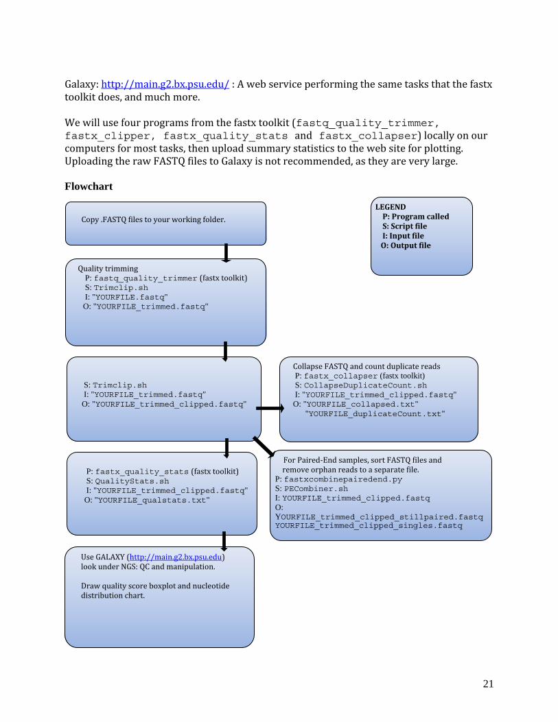
 Galaxy: http://main.g2.bx.psu.edu/ : A web service performing the same tasks that the fastx toolkit does, and much more.  We will use four programs from the fastx toolkit (fastq_quality_trimmer, fastx_clipper, fastx_quality_stats and fastx_collapser) locally on our computers for most tasks, then upload summary statistics to the web site for plotting. Uploading the raw FASTQ files to Galaxy is not recommended, as they are very large.  Flowchart

Copy .FASTQ files to your working folder. 

    Quality trimming  P: fastq_quality_trimmer (fastx toolkit) S: Trimclip.sh I: "YOURFILE.fastq" O: "YOURFILE_trimmed.fastq"

S: Trimclip.sh I: "YOURFILE_trimmed.fastq" O: "YOURFILE_trimmed_clipped.fastq"

LEGEND     P: Program called 

       S: Script file 

    I: Input file    O: Output file

P: fastx_quality_stats (fastx toolkit) S: QualityStats.sh I: "YOURFILE_trimmed_clipped.fastq" O: "YOURFILE_qualstats.txt"

 

      Use GALAXY (http://main.g2.bx.psu.edu)      look under NGS: QC and manipulation. 

 boxplot and nucleotide                Draw quality score      distribution chart. 

Collapse FASTQ and count duplicate reads  P: fastx_collapser (fastx toolkit) S: CollapseDuplicateCount.sh I: "YOURFILE_trimmed_clipped.fastq" O: "YOURFILE_collapsed.txt" "YOURFILE_duplicateCount.txt"

               

For Paired‐End samples, sort FASTQ file    remove orphan reads to a separate file. 

s and  

P: fastxcombinepairedend.py S: PECombiner.sh I: YOURFILE_trimmed_clipped.fastq O: YOURFILE_trimmed_clipped_stillpaired.fastq YOURFILE_trimmed_clipped_singles.fastq

                 

21

Process Download the data, uncompress and rename files.  1) a.   Find the files corresponding to your individuals on the sequencing center’s website, 

and download them into a new folder on your computer. b.   Use the sequencing center’s notes to rename the files to reflect your sample names. c.   Uncompress the .tar.gz files by double‐clicking on them in the finder window. d.   Change the file extension of the uncompressed files to .fastq if that is not already the 

case. e.  Study the .fastq format by opening a Terminal window, moving into the folder where 

the files are located with cd FOLDERNAME

then using the head command to display the top 10 lines of a randomly chosen file: head YOURFILE.fastq

2) Quality trimming and adapter clipping, using the bash scri .sh  

 rimClip.sh 

pt TrimClipfastq_quality_trimmer, fastx_clipper(fastx toolkit) P:

OURFILE.fastq files for each individuaS: TI: Y l O q file for each individual : YOURFILE_trimmed_clipped.fast

a.

Open the bash script in a text editor with 

edit ~/scripts/TrimClip.sh The bash script first invokes the quality trimmer, which scans through all reads, and when it encounters a base with a quality score of less than 20, trims off the rest of the read and then subsequently removes reads shorter than 20 bases. A file called YOURFILE_trimmed.fastq is created, which is then used as an input file for the ad apter seapter clipper. The clipper removes any read ends that match the defined adquences, and then removes reads that after clipping are shorter than 20 bases. 

b. For each step in the bash script, copy the lines to reflect the number of files (samples) that you are analyzing, change all the input and output file names, as well as the adapter sequences, in the bash script to match your data, then re‐save 

 quality score offset is not 64, you will need to oks like this: ‐Q QUALITYSCOREOFFSET  

the bash script. In addition, if youradd a flag to each command that lo

c. Execute the bash script by typing: TrimClip.sh

hile in the folder containing your data. Make note of how many reads are being wtrimmed and clipped through the screen output.  

3)   Calculate the fraction of duplicate and singleton reads, using the bash script Col pseDuplicateCounla t.sh.

 fastx_collapser(fastx toolkit), fastqduplicatecounter.py P:

individual S: C .sh I: YOURFILE_trimmed_clipped.fastq files for each O: YOURFILE_collapsed.txt files for each individual 

ollapseDuplicateCount

YOURFILE_duplicatecount.txt files for each individual

22

a. eOpen the bash script in a tedit ~/scripts/CollapseDuplicateCount.sh

The bash script first uses fastx_collapser to combine and count all identical reads.  A FASTA‐formatted file called YOURFILE_collapsed.txt is created, which is 

 

xt editor with 

then used as an input file for a python script (fastqduplicatecounter.py) thatcalculates the fractions of duplicate reads and singletons. 

b. For each step in the bash script, copy the lines to reflect the number of files that you are analyzing, change all the input and output file names in the script to match your 

(As above, you will need to specify the quality ser commands with the –Q flag if it is not 64.) 

data, then re‐save the bash script. score offset to the fastx_collap

c. Execute the bash script by typing: CollapseDuplicateCount.sh

while in the folder containing your data. d. Open the files named YOURFILE_duplicatecount.txt and note what percentage of 

your reads is duplicates, how many different sequences you have (unique reads) and how many singletons there are. Depending on the quality of your initial tissue and ample preparation procedure, the fraction of duplicate reads can be as low as 5‐s10% or higher than 50 %.  

4)   Summarize quality score and nucle tion data, and plot using the Galaxy web server. 

otide distribu

fastx_quality_stats(fastx toolkit) P:

individual 

 ualityStats.sh S: Q

I: YOURFILE_trimmed_clipped.fastq files for each  each individual O: YOURFILE_qualstats.txt files for

a. in a text editor with 

Open the bash script 

edit ~/scripts/QualityStats.sh TQ The bash script uses fastq_quality_stats to summarize the data in the FAS

file by read position (1‐50 or 101) into a file named YOURFILE_qualstats.txt b. Copy the lines to reflect the number of files that you are analyzing, change all the 

input and output file names in the script to match your data, then re‐save the bash specify the quality score offset for each of the nds with the –Q flag if it is not 64.) 

script. (As above, you will need to fastq_quality_stats comma

c. Execute the bash script by typing: QualityStats.sh

while in the folder containing your data.  d. Visit the Galaxy web server at http://main.g2.bx.psu.edu/. Upload the YOURFILE_qualstats.txt file under “Get Data” in the left panel. 

e. Plot it under NGS: QC and manipulation: Fastx Toolkit for FASTQ data. Choose files to plot under “Draw Quality Score Boxplot” and “Draw Nucleotide Distribution Chart” (you don’t have to wait for one plotting job to be done before starting the next one), then save the plots on your computer. They should look something like Figs. 2a‐b. If the mean quality scores are low throughout or if the nucleotides are non‐randomly distributed, something could have gone wrong during sample preparation or sequencing. 

23

5)  IF you have sequenced some or all of your samples with Paired‐End sequencing, you will for these need to sort your two FASTQ files so that reads are in the same order in both files, and so that any reads present in one file but not the other (“orphans”) get separated out into a separate file.  

P:S: 

URFILE_trimmed_clipped#1_1.fastq (

 PECombiner.sh fastxcombinepairedend.py 

I: YO YO:    OURFILE_1_trimmed_clipped_stillpaired.fastq

forward) OURFILE_trimmed_clipped#1_2.fastq (reverse) Y

ngles.fastq  YOURFILE_2_trimmed_clipped_stillpaired.fastq  

 YOURFILE_trimmed_clipped_si

a. in a text editor with Open the bash script edit ~/scripts/PECombiner.sh

The bash script uses fastxcombinepairedend.py to sort your two FASTQ files so that the reads who are in both files will be in the same order. It also removes 

ent in one file and saves them in another file. Notice that this HEADER and a DELIMITER argument in a s. 

all reads only presscript needs a SEQ

b. ddition to filename

In the Terminal, type head –n 1 YOURFILE_trimmed_clipped.fastq (Any of your files) 

to examine the format of the identifier line of your FASTQ files. SEQHEADER will be the first 4 characters of this line (including the @ symbol). DELIMITER will be the character separating the last part of the identifier (that tells the software if the read 

dentifier. It is usually either a “/” is a forward or reverse read) from the rest of the ior a “ “ (space) character. 

c. Enter your SEQHEADER and DELIMITER into the PECombiner.sh bash script, then copy the line to reflect the number of files that you are analyzing, change all the 

script to match your data and finally re‐save the input and output file names in the bash script. 

d.   Execute the bash script by typing: PECombiner.sh

while in the folder containing your data. This will create two FASTQ files with names ending in _stillpaired and one ending in _singles for each Paired‐End sample. These will be the files that you will use for downstream analysis (De novo assembly and mapping to reference) for your Paired‐End samples. 

24

Summary We have now cleaned up the raw data, so that they can be used for creating a de novo assembly or for mapping against a reference. Low quality bases and adapter sequences have been removed. We have also verified that the reads are not all identical, which would suggest an error somewhere in the sample preparation pipeline. We have also examined the trimmed dataset to make sure that quality scores are high and that nucleotides are evenly distributed. 

            

        Figure 2a. Quality score boxplot of 50‐bp Illumina reads (after quality trimming, Q>20), ummarized by read position. Lower scores in the beginning of the reads is an artifact of the oftware used to calculate base quality scores. ss                   

25

 Figure 2b. Nucleotide distribution chart of 50‐bp Illumina reads, summarized by read position. A non‐random distribution in the first 12 bases is common, and is thought to be an artifact of the random hexamer priming during sample preparation. 

2.  De novo assembly  Overview RNA‐Seq reads represent short pieces of all the mRNA present in the tissue at the time of sampling. In order to be useful, the reads need to be combined –assembled‐ into larger fragments, each representing an mRNA transcript. These combined sequences are called “contigs”, which is short for “contiguous sequences”. If you happen to be working with an organism for which there is a genome available, you can use the gene annotations to pull out sequences coding for mRNA and use those as the reference for further processing. If you already have a reference available, download it in the FASTA format and skip to section 4 (Mapping to reference). If not, however, you need to create your own catalog of contigs by performing a de novo assembly. A de novo assembly joins reads that overlap into contigs, while allowing a certain, user‐defined, number of mismatches (variation at nucleotide positions that can be due to sequencing error or biological variation). 

Contig Short reads

             Figure 3. Example of a contig assembled by the joining of many short reads.  

 When comparing the lengths and numbers of contigs acquired from de novo assemblies 

to the predicted number of transcripts from genome projects, the de novo contigs typically are shorter and more numerous. This is because the assembler cannot join contigs together unless there is enough overlap and coverage in the reads, so that several different contigs will match one mRNA transcript. Biologically, alternative splicing of transcripts also inflates the number of contigs when compared to predictive data from genome projects. This is important to keep in mind, especially when analyzing gene expression data based on mapping to a de novo assembly. To minimize this issue, we want to use as many reads as possible in the assembly to maximize the coverage level. The assembler therefore pools the reads from all specified samples, which means that no information about the individual samples can be extracted from the assembly. In order to get that information, we need to map  from e  

26

 our reads ach sample individually to the assembly once it has been created(section 4). 

Building a de novo assembly is a very memory‐intensive process. There are many programs for this, some of which are listed in the Resources section of this chapter. In our experience, the one that can be used most effectively on any fairly new Mac computer is CLC genomics workbench, as most others require more RAM memory than typically is available 

on personal computers (in the 100’s of GB, depending on the number of reads). CLC is the only software in this protocol that is not open source (an academic license is currently $4,995), although there is a free two‐week trial version available. Unlike the other software in this protocol, CLC has a point‐and‐click graphical user interface and is very easy to use. CLC uses De Bruijn graphs to join reads together. More information about how the assembly algorithm works can be found here: http LC://www.clcbio.com/files/whitepapers/white_paper_on_de_novo_assembly_on_the_C_Assembly_Cell.pdf 

The parameters we use in this protocol have proved to work quite well for our data. evertheless, it is useful to try to perform several assemblies with your dataset, with arying parameter values (especially the mismatch costs), to see how the results differ. Nv Objectives The objectives of this section are to 1) import our reads into CLC, 2) build a de novo ssembly, 3) examine the properties of the newly‐created assembly, and 4) export our ssembly from CLC. aa esources 

id=1240RCLC genomics workbench: http://www.clcbio.com/index.php?   Examples of other available software for short read assembly: Trinity: http://trinityrnaseq.sourceforge.net/ 

sABYSS: http://www.bcgsc.ca/platform/bioinfo/ oftware/abyss Velvet: http://www.ebi.ac.uk/~zerbino/velvet/ Oases: http://www.ebi.ac.uk/~zerbino/oases/  Her ackagese’s also an excellent review describing and contrasting the different software p  in use: 

Zhang W, Chen J, Yang Y, Tang Y, Shang J, et al. 2011. A practical comparison of de novo enome assembly software tools for next‐generation sequencing technologies. PLoS ONE 6: 17915. doi:10.1371/journal.pone.0017915 ge  Process 1) TQ files into CLC. Import the quality‐trimmed, adapter‐clipped FASa.   Open CLC b.   Import your _trimmed_clipped.fastq files to CLC: 

File -> Import High-Throughput sequencing data -> Illumina  2) de novo assembly. 

Toolbox -> HigSelect all samples. 

a. h-Throughput sequencing -> de novo Assembly

b. Specify mapping parameters: Mismatch cost 1. Limit 5. Uncheck “fast ungapped alignment”. Insertion and Deletion costs: 2 (no global alignment)

27

Mismatch costs determine how many nucleotide mismatches are allowed before the reads can’t be joined together. A mismatch limit of 5 allows 5 out of 50 = 10 % difference or 2 indels (as they cost 2 penalty units each). Vote for conflict resolution. Ignore non-specific matches. The former prohibits ambiguities in the contigs, and instead uses the most common nucleotide. The latter option ignores all reads that match to more than one contig. As we cannot know which contig they belong to, it is safest to ignore them. Minimum contig length 200 bases. Map reads back to contigs and update contigs based on mapped reads. This option makes the assembly considerably more time­intensive and can be ignored if you are pressed for time. However, the assembly can be improved by matching reads to 

rtant to have as good as possible an assembly cking this option. 

it one extra time, and as it is very impofor downstream analysis, we recommend cheCreate summary report and save log. 

. c 

Complete the assembly by clicking “finish”. 

3)  To further study the results of the assembly, create a detailed mapping report. a. Toolbox -> High-Throughput sequencing -> Create detailed mapping report b.  Study the mapping report, especially the contig length distribution, proportions of 

reads used and coverage distributions. In most cases there will be a few contigs with high and many with lower coverage. The more reads that are included in the assembly, the longer (and perhaps fewer) the contigs will be, as they better will represent complete mRNA transcripts. 

 4) Export your newly created reference assembly in the FASTA format, and rename the

contigs. FASTA files contain 2 lines per sequence, one identifier line, starting with >, and line. C e name of the first inone sequence LC names all contigs with th put file, plus a

number. We want to change the names to something simpler, such as “contig#” a. Select your de novo assembly in the left panel. File -> Export, choose FASTA format and .fasta as file extension, save in the folder containing your project. 

b. Now, open your .fasta reference assembly in TextWrangler, and Find‐Replace the ontig names with something simpler. Make sure that the contig numbers remain, to eep each contig identifiable. ck 

Summary We have now created a de novo assembly, which we will use as a reference for downstream analysis. The assembly only contains information about contig sequences, and no information about how many reads were used to create them or what samples they came from. The assembly is a proxy for a library of all mRNA transcripts present in the tissue at the time of sampling, although several contigs could belong to different parts of the same mRNA molecule. In the assembly, we allowed for 5 mismatches in any one read (about 10%), ignored reads that matched to more than one contig, and set a minimum contig length of 200 bases. 

28

3a. BLAST comparison to known sequence databases and functional nnotation 

 Overview Establishing links between observed sequence variation and gene function is a major challenge when analyzing transcriptome data from non‐model organisms. Here, the Basic Local Alignment Search Tool (BLAST) is used to compare your de novo assembled contigs to sequence databases in order to annotate them with similarity to known genes/proteins/functions. BLAST is a toolkit developed by the National Center for Bio d technology Information (NCBI), the US‐based organization responsible for archiving andatabasing the world’s genetic sequence information. 

By querying three major databases, GenBank’s non‐redundant protein database (NR) and Uniprot’s Swiss‐Prot and TrEMBL protein databases, we will identify the most similar known sequences for each of our contigs. The available information about these matching sequences will be used to annotate our contigs with likely functional properties. For the significant matches in the database, we will extract both gene names, general descriptions, and Gene Ontology (GO) categories (specific categorical classifications grouping genes based on cellular and molecular function, e.g. “cellular response to protein unfolding” or “calcium homeostasis”), along with additional information from the Uniprot knowledge database. GO categories will also be used in step 5 for the functional enrichment analysis. 

A note on E­values To determine whether matches to the databases are “significant”, we use a threshold E‐value. The E‐value describes the number of hits one can expect to see by chance when searching a database of a particular size. The lower the E‐value, the more "significant" a match to a database sequence is (i.e. there is a smaller probability of finding a match just by chance). However, the quality of a match also depends on the length of the alignment and the percentage similarity, so these statistics may also be considered when evaluating the significance of a match. In the following steps there will be two thresholds employed: the first is a liberal threshold that is used during the BLAST search itself (generally 0.001) which serves to eliminate very bad matches from the raw BLAST output, the second is a more stringent threshold to identify very good matches (generally 1E‐4 or below) that is used to parse out the top “hits” from the raw BLAST output for further annotation. Neither of these thresholds are set in stone; however, an E‐value of 1E‐4 or below seems to be commonly acceptable in the literature for diagnosing a “good” match.

Objectives The objectives of this section are to 1) retrieve the best matches in the NR and Uniprot atabases for our assembled contigs, and 2) create a metatable that summarizes the vailable annotation information for each contig. da     

29

Resources  BLAST: Basic Local Alignment Search Tool.  ftp://ftp.ncbi.nlm.nih.gov/blast/executables/LATEST/ The  your se tools should have been installed on your computer during the “How to set upcomputer section” 

The BLAST executables comprise multiple programs to compare a set of query sequences (in the FASTA file format) to a pre‐formatted database on you computer. Here e will use the blastx tool that searches a nucleotide query, dynamically translated in all six eading frames, against a protein database. wr Sequence databases A wide n the web, but here we will limit ou

 variety of searchable databases are publicly available o

r search to three major repositories: NR:

The :  NCBI’s non‐redundant protein sequence database  Uniprot protein knowledgebase, which consists of two sections

Swiss‐Prot, which is manually annotated and reviewed.  TrEMBL, which is automatically annotated and is not reviewed. 

Generally, Swiss‐Prot should provide the most conservative, verified, and up‐to‐date sequence information and functional role identification. If a given sequence finds no significant match in Swiss‐Prot, then the TrEMBL and NR hits may be used to infer fun ill usually be less ctional annotation, but entries in these more broad databases w

ee informative. 

n GenBank and Uniprot databases, sov/staff/tao/URLAPI/blastdb.html

For more information ottp://www.ncbi.nlm.nih.gh  http://www.uniprot.org/  

30

A note about BLASTing against very large databases BLAST comparisons against very large databases (e.g. NR or TrEMBL) can often take ~30sec to 1min per query sequence. When you have 100,000 query sequences, this can add up to multiple days, weeks or even months of run‐time, even when you employ the multiple‐core option of BLAST. An alternative approach is to use a computer cluster to run multiple BLAST jobs at the same time. For example, say we have a de novo assembly of 100,000 contigs. If we run 1 BLAST job against NR it could take as long as 50,000 minutes/35 days!! (30sec/query sequence), however if we split this job into subsets of 5,000 sequences and ran 20 jobs in “parallel” on a cluster, our total run‐time is reduced to only 41 hours. There are commercially available clusters that have a fee‐for computation type structure (e.g. the amazon cloud http://aws.amazon.com/ec2/) and many universities have clusters available in‐house as well. You’ll need a simple Terminal‐based capacity and may need to install the BLAST toolkit (just like you did on your desktop) onto the cluster computer. Alternatively, there are a few web‐based BLAST services that provide parallel BLASTing for free for users in academia (e.g. the University of Oslo bioportal http://www.bioportal.uio.no/) and can generally run a large BLAST to NR in a couple of weeks. Smaller BLAST searches are most efficient when run locally on your desktop. 

De novo assemblies generated with the test files (containing 458 contigs of mean length 421 bp) supplied with this guide should take ~20 min to BLAST against Swiss‐Prot and about 10 hours for TrEMBL and NR when run on a standard desktop Mac.  

  Flowchart                                        

31

P cro ess ar 3.1) P t  1: BLAST contigs against the three databases 

Download and format the databases. a. Create a folder for each of your reference databases. You can either run all your 

BLAST jobs from within these folders (which will require you to copy all your query ath to these databases in every files into the same folder) or you can specify the full p

run. b. Download the the NR database in .fasta format from 

ftp://ftp.ncbi.nih.gov/blast/db/FASTA/ and the Swiss‐Prot and TrEMBL databases in .fasta format from http://www.uniprot.org/downloads (note that the uncompressed NR and TrEMBL databases are very large (7‐8 GB) and that BLAST searches to these take a long time. See Box 3.1 for alternative ways to process large BLAST jobs). 

c. In Terminal, change your working directory to the folder where you saved the three fasta database files (cd FOLDER PATH) and format them into BLAST protein atabases using the program makeblastdb by typing: .d makeblastdb -in DATABASENAME.fasta -dbtype prot \ -out DATABASENAME

 Replace the words in capital letters with the relevant database names. The –in parameter specifies the name of the .fasta file that contains the sequences you want to format, e.g. uniprot_trembl.fasta; ‐dbtype specifies whether you are dealing with a nucleotide or protein database (here we only work with protein databases); and ‐out 

t to use for your formatted database. specifies the name you wan

2)  

Familiarize yourself with the Blastx tool. a. To get an overview of how this program works and which arguments and parameter 

values you can input, take a look at the help page, which you open in Terminal by typing:  blastx –-help

3) n will BLAST the contigs from your de novo assembly against NR (Note: this computatio

likely take hours to days to complete, see box 3.1). a. Copy your de novo assembly .fasta file to the folder containing your formatted 

l, make sreference database. In Termina ure that this folder is your working directory. 

b. Start your BLAST job using the blastx tool, by replacing the words in capital letters (except the BLOSUM62 which is a specific BLAST parameter) with your own sample names and typing into Terminal:  blastx -query YOURASSEMBLY.fasta -db DBNAME \ -out YOURASSEMBLY_BLASTX2DBNAME -outfmt 5 -evalue 0.0001 \ -gapopen 11 -gapextend 1 -word_size 3 -matrix BLOSUM62 \ -num_descriptions 20 -num_alignments 20 -num_threads 4

32

The ‐query is the input file name, e.g. testfile_assembly.fasta; ‐db is the name you gave to your formatted BLAST database in step 1, e.g. NR (note that you should not specify the extensions for the formatted database file names (.phr, .pin and .psq) only  the given name of the file); ‐out is the name you want for your output file, e.g. testfile_blastx2NR; ‐outfmt specifies the format for how the program outputs the results (for further processing in this pipeline we need option 5, the xml format; –evalue is the expectation value (E) threshold for saving hits (see the description in the beginning of this chapter; your choice should depend on how stringently you want to exclude potential chance matches); ‐gapopen, –gapextend, word_size, and –matrix specify parameters for the alignment algorithm (see http://www.ncbi.nlm.nih.gov/BLAST/blastcgihelp.shtml for details); ‐num_descriptions and ‐num_alignments are the number of matching sequences in the database to show one‐line descriptions and alignments for, respectively (you can choose any number up to 500 and 250, respectively, but in part 3 here we will only extract the top hit); ‐num_threads is the number of threads the BLAST search should use (depends on how many processors/cores your computer runs on). In the erminal, the command uname –a will indicate the number of threads at your Tdisposal.  For many of the parameters, we use the default values from the NCBI web‐based BLAST searches. However, to keep track of analysis settings, we have found it helpful to specify these parameters with every search as different versions of the stand‐lone BLAST toolkit may have different default parameters. Feel free to modify these, abut the parameters specified here should provide a good starting point. 

4)  

Blast the contigs from your de novo assembly against Swissprot and Trembl. a. Follow the instructions in step 3, but this time selecting the formatted Swissprot and 

rembl databases (one at the time) and choosing output format 7 which corresponds o a tabular format that we will need for further processing: Tt blastx -query ASSEMBLY.fasta -db DBNAME \ -out ASSEMBLY_BLASTX2DBNAME -outfmt 7 -evalue 0.0001 \ -gapopen 11 -gapextend 1 -word_size 3 -matrix BLOSUM62 \ -num_descriptions 20 -num_alig

5)

nments 20 -num_threads 4

Parse the results from your BLAST against NR   the .xml a. In Terminal, make sure you are working from the directory that containsformatted output from your BLAST against NR 

b. Parse the output to tabular format (one line for each hit) with the script parse_blast.py. Replace and names in capital letters with your own file names and type in Terminal: parse_blast.py YOURASSEMBLY_PARSEDblastx2nr.txt \ YOURASSEMBLY_blastx2nr

 where the first argument following the script name is the name you want for the parsed output file and the second argument is the name of your .xml-formatted BLAST output. This generates a list for all the hits found for each contig (given the restrictions you

33

specified in step 1). On rare occasion, the parse_blast.py script may not function correctly. If this is the case we have included an alternative parsing script for backup use (BlastParse.pl). Usage for this script is as follows: BlastParse.pl YOURASSEMBLY_blastx2nr.xml >> \ YOUR_ASSEMBLY_PARSEDblastx2nr.txt 

 Part 3.2: Annotation of sequences and metatable generation In part 1, you identified significant matches between your contig sequences and known proteins in the nr and Uniprot databases. In this part, we have developed an automated pipeline which will: (a) combine the blast results from the three databases, (b) download the associated Uniprot flatfiles from the uniprot.org website (you will need an active internet connection for this script to work), (c) extract additional information about each of these matching proteins, including a description of their function and their associated GO ategories, and (d) combine all available annotation information into a master annotation cmetatable.  1) Make sure that your query sequence .fasta file (your de novo assembly) and the output 

files for the Swissprot, TrEMBL, and parsed NR BLAST searches are in the same folder and make this your working directory in Terminal.  

2) In this step, we have automated a lot of different processes, thus, pay careful attention to the specific order and the specifications for each input file. You will need to generate a short companion file called “nrcolumnheadersandbadwords.txt” to specify the names of the description and evalue columns generated during parsing and a customizable list of “bad words” that you can exclude during final combining of the nr results. Due to the size of the nr database, many top hits for non‐model systems will be uninformative (e.g. “predicted protein”), so we have built in a second column in the meta table that includes a lower hit when possible for these contigs that excludes the “bad words”. Execute the otalannotation.py script in Terminal by replacing the words in capitals with your own ile names and typing: tf 

totalannotation.py YOURASSEMBLY.fasta \ YOURASSEMBLY_Parsedblastx2nr.txt \ nrcolumnheadersandbadwords.txt \ YOURASSEMBLY_blastx2sprot.txt \ YOURASSEMBLY_blastx2trembl.txt \ 1E-4(or other evalue cutoff) UniProt_flatfiles \ YOURASSEMBLY_annotated.txt

YOURASSEMBLY.fasta is your de novo assembly contig file, e.g. testfile_assembly.fasta; YOURASSEMBLY_Parsedblastx2nr.txt is the parsed nr .xml file with each hit on one line;  nrcolumnheadersandbadwords.txt are the column names corresponding to the match description and evalue on one line (e.g. “HitDescription” and “eValue”) and a list of “bad words” that you want to skip over to find an informative nr match (e.g. “hypothetical”, “Predicted”, “unknown”) all separated by tabs; YOURASSEMBLY_blastx2sprot.txt is the output file from the BLAST of your contigs against Swiss‐Prot, e.g. testfile_blastx2sprot; YOURASSEMBLY_blastx2trembl.txt is the .txt output file from the BLAST of your contigs 

34

against TrEMBL, e.g. testfile_blastx2trembl ; 1E‐4 is the threshold specifying that only BLAST hits with an E‐value below this will be annotated; UniProt_flatfiles is the name  or the folder that will contain the flat files for the matches in Swiss‐Prot and TrEMBL; ‐fand YOURASSEMBLY_annotated is the name you want for your output file.  

3) Open the output file as a text file or in a spreadsheet and review your annotation information. 

 Summary You should now have a complete metatable summarizing annotation information for those of your contigs that matched known proteins in the queried databases. This provides a convenient overview of the top hits from the different databases, summarizes functional annotation information, and generates some of the input required in subsequent analyses (e.g. the GO functional enrichment analysis in step 5). While this annotation table is a good summary, since many contigs can have multiple BLAST matches, it can also be useful to look at the full list of BLAST results for certain contigs. Additionally, if a particular contig of interest does not result in any siginificant matches in the annotation process, hand‐curated BLAST‐ing via the NCBI web‐interface may also provide additional sequence identification information.  

35

Section 4. Mapping reads to a set of reference sequences  

Overview Mapping refers to the process of aligning short reads to a reference sequence, whether the reference is a complete genome, transcriptome, or de novo assembly. There are numerous programs that have been developed to map reads to a reference sequence that vary in their algorithms and therefore speed (see Flicek and Birney 2009 and references therein). The program that we utilize in this pipeline is called BWA (Li and Durbin 2009).  It uses a Burrow’s Wheeler Transform method that results in much faster processing than the first wave of programs that used a hash‐based algorithm such as MAQ (Li et al. 2008). The goal of mapping is to create an alignment file also known as a Sequence/Alignment Map (SAM) file for each of your samples. This SAM file will contain one line for each of the reads in your sample denoting the reference sequence (genes, contigs, or gene regions) to which it maps, the position in the reference sequence, and a Phred‐scaled quality score of the mapping, among other details (Li et al. 2009). You will use the SAM files for your samples to extract gene expression information (the number of reads that map to each reference sequence) and to identify polymorphisms across your data. 

There are several parameters that can be defined for the alignment process, including: the number of differences allowed between reference and query (‐n), the number of differences allowed in the seed (‐k), the number allowed and penalty for gap openings (‐o, ‐O), and the number and penalty for gap extensions (‐e, ‐E). Changing these parameters will change the number and quality of reads that map to reference and the time it takes to complete mapping a sample. For a complete list of the parameters and their default values go to http://bio‐bwa.sourceforge.net/bwa.shtml. To optimize the parameters for your data, i.e. to obtain the highest number of high quality mapped reads, you should generate an evaluation data file (cleaned and trimmed FASTQ file from a single sample) that you can use to run through several permutations of bwa, changing a single parameter each time.  You can use the counts script from the gene expression section of this pipeline to see the number and quality of reads mapped with each set of parameters. The number of nucleotide differences (‐n) is probably the most important mapping parameter to fine‐tune for your data. This should match the expected number of differences between two sequences for your species. n can be an integer (maximum edit distance, in other words the number of changes needed to convert one string to another, e.g. 5) or a fraction of missing alig e nments given a 2% uniform base error rate (e.g. 0.04). Counter intuitively, the larger thfraction, the fewer mismatches allowed and visa versa. 

Terminology: Seed – a stretch of nucleotides within a read that are used to initiate the alignment process. Phred‐scale – a number scale often used for quality scores; given a p‐value ranging from 0 to 1 (probability of the mapping being incorrect), the Phred score is ‐10*log10p, rounded to the nearest integer. 

36

 Objectives In this section, we will map the reads from each of your cleaned and trimmed FASTQ files from Section 1 of this guide to the de novo reference assembly that you created in Section 2 of this guide (or the predicted genes if your study species has a genome sequence). Specifically, we will 1) create an index for the reference assembly (just once), 2) for each sample, map reads to the reference assembly, and 3) convert the resulting file into the SAM 

file format and append “read group” names to the SAM file for each sample. Steps 2 and 3 are “piped,” or put together feeding the output of one program in as the input for the next program. The read groups, which can have the same names as your sample names, will be appended to each file and will become critical for the downstream SNP detection step. The read group name in each SAM file will connect the reads back to individual samples after files have been merged for SNP detection. All of the above steps for all samples can be “batch” processed at once by editing the bash script BWAaln.sh. We then want to remove all duplicate reads, for which we need to use the MarkDuplicates program from the software package “Picard”. Picard uses the binary equivalent of SAM files, BAM, as input, so first we need to convert the files using SAMtools. These steps are performed by the convert_to_BAM_and_dedup.sh bash script. 

 

urcefourge.netResources 

wa.soBurrows‐Wheeler Aligner (BWA) – available at: http://bio‐b  SAM file description ‐ http://samtools.sourceforge.net/SAM1.pdf SAMtools ‐ http://samtools.sourceforge.net/samtools.shtml 

Flicek, P, Birney, E. 2009. Sense from sequence reads: methods for alignment and assembly. Nature methods 6:S6‐S12. 

r Li, H, Durbin, R. 2009. Fast and accurate short read alignment with Burrows‐Wheeletransform. Bioinformatics 25:1754‐1760. 

Li H, Handsaker B, Wysoker A, Fennell T, Ruan J, Homer N, Marth G, Abecasis G, and Durbin R. 2009. The sequence alignment/map format and SAMtools. Bioinformatics 25: 2078‐2079. 

Li, H, Ruan, J, Durbin, R. 2008. Mapping short DNA sequencing reads and calling variants using mapping quality scores. Genome research 18:1851‐1858. Picard tools: http://picard.sourceforge.net/ : Java‐based programs for manipulation of .sam and .bam files. 

 cess

1. Open the BWAaln.sh script in TextWrangler using Finder or from Terminal, by moving ipts folder and typing:

Pro

to the scr eor type: 

dit BWAaln.sh

edit ~/scripts/BWAaln.sh

2.  Edit your file names for your reference, samples, and the “read group” names (in pink font in the script if you are using TextWrangler with default settings, these can be the same as your sample names and are important for linking alleles to specific sample files in your downstream SNP analyses). The –I flag to each bwa command tells the program that you are working with Illumina reads with a quality score offset of 64. If you have data with a quality score offset of 33, this flag can be removed. Note also that if you are analyzing Paired‐End samples, there are 4 lines per sample, first aligning the singles file and each of the stillpaired files separately, and then combining the paired files into one alignment file (The singles file will be combined with the others in the merging step at the end of this section). 

 

37

3.  Move into your working directory where your reference and sample files are (or specify the complete path to these files in the BWAaln.sh script).

4.  You may want to make a smaller evaluation file with which to test alignment parameters, particularly those described in the overview. Type: 

head –n 10000 SAMPLENAME.fastq >> SAMPLENAME_head.fastq Note that the double arrow (“>>”) will create or append to an existing file that has the same name. It can be safe practice to use “>>” rather than “>” so that you do not overwrite an existing file (but may also result in unintended extra appended data in a file, so always pay ttention). a

  You can examine the effects of the different parameters by using the countxpression.py script described in Section 5 on Gene expression. By changing mapping parameters with your test file, you will see differences in the number of multiply (to many contigs) and singly (to one contig) aligned reads, and in the time required to process the file. In general, you want to maximize the number of reads mapped singly and minimize computing time. You should have at least 50% of your reads mapping to at least one contig (column called FracAligned in output file) and hopefully around 70% of you read  s that map should map to a single contig (column called FracSingleOfAligned in outputfile). But mapping results may be very species specific. 

5. Make sure that your input and output file names, as well as the read group headers are correct, then execute the script by typing: 

BWAaln.sh 6.  When the computer has finished mapping, we want to see what the .sam file format looks like. We can easily view the bottom 50 lines of a file using the very useful bash command tail”. Type: “

tail SAMPLENAME.sam –n 50  See the pdf in the link provided in the resources above for details on the SAM file format. Note that the text for each line will wrap around; you can make your Terminal window wider to fit more of read row on a single line. Generally, what you will see is a row for each read and many columns of data associated with each read. The first column is a string of the read name or “query template name”, the second column will tell you if the read mapped anywhere (e.g. “4” did not map, “0” or “16” did map), the 14th column will tell you if the read mapped to one or many contigs (if the number after the second colon is “1” then it mapped to one contig, if it is greater than “1” than it mapped to more than one contig). The 3rd column tells the reference contig name to which the read maps (or first mapped). The 4th column tells the first position relative to the reference where the read maps. The 5th column tells the mapping quality and is Phred‐scaled (see overview). The 10th column gives the equence of the read and the 11th column gives the ASCII of the base quality plus 33 (also hred‐scaled as described in the overview). sP   

38

   7. Convert your .sam files to .bam, sort and remove duplicate reads. Open the convert_to_bam_and_dedup.sh script in TextWrangler and input your sample names as in‐ and output files (add lines for each additional file), then re‐save the script. The convert_to_bam_and_dedup.sh script has 2 elements: 1) It converts the sam file to a binary bam file and sorts the reads within it. 2) It marks and removes uplicate reads using the MarkDuplicates program from the Picard package. .d   Summary You have mapped each of the cleaned data files to a reference assembly to generate an alignment file for each sample. You have also removed all duplicate reads from the dataset. You are now ready to move on to gene expression analyses or SNP detection. 

39

5.  Gene expression analyses from RNA­Seq data  Overview In this section we will extract count data ‐ the number of reads that map uniquely to each contig or gene ‐ from the alignment files that you generated for each sample in Section 4. The count data will serve as a proxy for the magnitude of gene expression since transcripts of greater abundance in the cell will have more reads generated from libraries prepared from RNA. Gene expression may vary among samples or individuals in your study due to your experimental design, for example control versus heat shock or high versus low intertidal zones. The biological questions you can address using the analyses below include: How many genes, if any, are differentially expressed between my treatments? Are diff  erentially expressed genes concentrated in specific functional types of genes or are theyrandomly distributed with respect to function across the transcriptome?  

In the analyses described below, we consider only the reads that map to only one place across the entire reference. There are a number of reasons a read may map to multiple reference sequences such as sequence similarity due to gene duplications or homologous regions across gene families, or errors in the generation of the reference sequences considering one gene as two genes. It is not possible to distinguish between the ossibilities, so the most conservative approach is to only consider the reads that map to ne contig or gene. po Objectives The objectives of this section are to 1) convert our deduplicated .bam files back to .sam, 2) extract count data from the mapped reads for each individual (.sam files), 3) make a combined counts data file for all individuals in the gene expression study (a column for each sample and a row for each gene), 4) normalize across individuals and identify significantly differentially expressed genes using the program DESeq implemented in R, and 5) use p‐values from DESeq to identify ‘transcriptome’‐wide patterns of enrichment for functional classes of proteins using the software ErmineJ.  Resources DES  on the

eq: Gene expression data analysis program.  There is a very useful manual available website. http://www‐huber.embl.de/users/anders/DESeq/ nders, S, Huber, W. 2010. Differential expression analysis for sequence count data, A

Genome Biology 11: R106 

Er mineJ: http://www.bioinformatics.ubc.ca/ermineJ/     The website is very informative. The link below describes the four input file formats.     http://www.bioinformatics.ubc.ca/ermineJ/ermineJ‐help/classScore/html/formats/ 

 he website called Quick‐R (T http://www.statmethods.net/ ) provides basic information for learning how to code in the R environment.  In this pipeline, we use the program DESeq (Anders 2010) to normalize counts and test for differences in gene expression. However, there are many other programs that perform 

40

similar functions. (e.g. EdgeR and BaySeq (Hardcastle and Kelly 2010, Robinson et al. 2010)).  Hardcastle, T, Kelly, K. 2010. baySeq: Empirical Bayesian methods for identifying 

differential expression in sequence count data. BMC bioinformatics 11: 422. Robinson MD, McCarthy DJ, Smyth GK. 2010. edgeR: a Bioconductor package for differenti

expression analysis of digital gene expression data. Bioinformatics 26: 139. Wang Z, Gerstein M, Snyder M. 2009. RNA‐Seq: a revolutionary tool for transcriptomics. 

Nature Reviews Genetics 10: 57‐63. 

al

Process  1) C am. onvert your deduplicated .bam files from section 4 back into their text equivalent, .s

a.   In Terminal, change your working directory to the folder containing your /FOLDER). Tip: drag and drop folder from ath 

deduplicated .sam files (cd PATH/TOfinder rather than typing out the full p

b.  Convert .bam to .sam using SAMtools:   up.sam samtools view –h FILENAME_dedup.bam > FILENAME_ded

ct count data from the  2) Ex d duplicated .sam file from each individual using          the ountxpression.py script. Execute the script from the Terminal shell. 

tra e

  c

AMPLENAME_dedup.sam fiP: countxpression.py: S les for each individual 

AME_counts.txt file xt IO: SAMPLEN  for each individual; counts.t 

a.    Execute the countxpression.py script from the Terminal shell.   countxpression.py 20 20 summarystats.txt *.sam

The first argument is the mapping quality threshold, the second argument is a length threshold, summarystats.txt is an output file combining count statistics from all files. The last argument tells the program to count reads from all .sam files in the folder. 

b. Take a look at the summary stats output. What fraction of your reads mapped to only one place in the assembly? We have seen that approximately 70% of the reads that 

 

map do so to only one reference sequence (column called FracSingleOfAligned).  3)  Extract the second column of data (number of unique  eads mapped to each contig) from 

the counts file from each individual. r

arseExpression2 igTable_counts.py S: PI: CO

BontigNames.txt, FILENAME_counts.txt files for each individual 

: CombinedCounts.txt 

a. Put all your FILENAME_counts.txt files into one folder b. Change your working directory to that folder (cd PATH/TO/FOLDER) c. Make a file that is a list of all your contig names called ContigNames.txt and the 

first row called ContigName. 

41

d. Execute the ParseExpression2BigTable_counts.py script from the Terminal shell. Note that the wildcard “*” will tell the script to process all files in your current working directory whose name ends with “counts.txt”. 

ParseExpression2BigTable_counts.py ContigNames.txt \ CombinedCounts.txt *counts.txt

e. Alternatively, if you are only dealing with a few files, you can open each one and copy and paste the second column using Excel. The script has the advantage of grabbing the correct column each time and labeling the column with the input file 

name.  4) Identify differentially expressed genes using the program DESeq.  In this section you will 

work in the R programming environment executing sequential parts of a script file. It is useful to move through the script a few lines at a time in order to learn about your data and to realize what each step of the script does. 

a. Open R and open the DESeqScript.R script file from inside R. b. In the DESeqScript.R script, change the working directory (the drag and drop trick 

works in R, too), enter your input file name (likely CombinedCounts.txt if you successfully used the script from step 2), enter your conditions (e.g. hot and cold, or whatever your conditions are for each of your samples). There should be a named condition for each of the samples or columns of data in your file, i.e. each condition 

 in your input file (theycorresponds to a column of data  need to be in the same order). 

c. Run the script through the line head(countsTable) by highlighting the lines and You should see the firsentering apple+return.  t 6 rows for each of your columns in 

the table populated by your input file. d. Run the script through sizeFactors(cds). The calculated size factors are factors 

such that values in a column can be brought to a common scale by dividing by the corresponding size factor. Ideally you want all of the factors near 1. If you see a 

, then there w   reads for th

factor much less than 1 ere many fewer singly mapped reads for thatsample and likely fewer at sample, and visa versa. 

e. Run the script through head(res). You should see the output columns from the results table. 

f. Run the script through counting the number of significantly differentially expressed genes (the line that begins with the nrow function). You should see how many differentially expressed genes you have in your data set based on these conditions and at the p < 0.05 and p < 0.01 significance levels. 

g. Run a few more lines of script to filter out the contigs where the average number of counts is less than 5. This filter may affect the number and fraction of significantly differentially expressed genes. 

h. Now filter your results excluding contigs that have high variance (down to line ~73).  Step through the lines stopping at the head and dim functions to follow how the data are being processed. 

i. Now you can change the file names and generate various output items to be used for further analyses (lines ~76‐110). 

42

j. You can also make a heat map of your significantly differentially expressed genes using the heatmap.2 function from the gplots library in R. You can install gplots from within R: Go to “Packages & Data,” “Package Installer,” search for gplots, select it and “install dependencies,” then click “Install Selected.” Note that you need to be connected to the internet. To make the plot you should normalize each gene to itself, i.e. divide the counts for each individual by the average counts across all individuals – essentially relative fold difference. This will make all genes visible on a single plot even if some have two orders of magnitude higher counts, for example.  You can make this new data matrix in R or Excel and save it as a .txt file. Now open the R script Heatmapping.R. Run the lines of the script sequentially as you did in the script above. Note that you will need to change the value of n in line 12. You can save the heat map image from Quartz in R though the quality is poor or you can press apple+shift+4 to capture a nice image of your heat map (it will save to the desktop by default). Or you can write a script in R to save a higher quality image. 

5)  Test for functional enrichment across your gene expression data using ErmineJ and your 

outputs from DESeq.      Ermi J ne requires 4 input files: 

 1. GeneScores.txt – usually either p‐values or “fold‐change,” file format must be 1stcolumn ContigName, 2nd column ContigScore, one header line 

2. GeneExpressionProfiles.txt – This is optional but useful for visualizing the data. b t nts data 1st column – ContigName, su sequen  columns are the normalized cou

for each of your samples output from DESeq. 3. GeneAnnotations.txt – The 1st and 2nd columns are the ContigName, 3rd column is 

annotation description of the gene (from blastx to nr or uniprot), and the 4th column is a delimited list (comma, space or pipe) of GO identifiers (e.g. 

e GO:00494494,GO:00345678). These identifiers are generated during thannotation process in Section 3. 

4. nsortium website aily‐termdb.rdf‐xml.gz

Gene Ontology XML file – downloaded from the GO cohttp://archive.geneontology.org/latest‐termdb/go_d  An updated link is provided on the ErmineJ website. 

a. Create files 1‐3 using Excel from your DESeq outputs and your outputs from the 

annotations you did in Section 3.  et or open it if you downloaded it in the Set up your 

s.ubc.ca/ermineJ/webstart/ermineJ.jnlpb. Download the ErmineJ java appl

computer section (http://www.bioinformatic ) c. ‐ Sta

‐ Loart the ErmineJ application;  d the GO XML and GeneAnnotation files The table and tree show two views of the number of genes you have in each functional category. 

core distribution rather than a ‐ Run a Gene score resampling analysis (uses the whole scutoff): Analysis ‐> Run Analysis ‐> Gene score resampling ‐ Select your GeneScore and GeneExpressionProfile files ‐ Click Next, unless you have created custom gene sets to include  

43

‐ Consider just the Biological Process (at least initially as this is usually most interesting) ‐ Maximum gene set size: 100, Min: 10, functional categories with more that 100 genes are too general and ubiquitous while categories with less that 10 genes will be statistically inaccurate. ‐ Take the negative log of gene scores if dealing with p‐values; Larger scores are better only if your GeneScores are fold differences (ie. greater differences between treatments are more interesting); choose 10,000 iterations to explore the data and 200,000 iterations and full resampling to publish. Now click “Finish.” 

d.  You should see if there are any functional categories that are enriched for differentially expressed genes (after correcting for multiple tests ‐ green). You can 1) explore the results in the table and tree views, 2) double click on a category to see the genes and expression profiles of the gene members of a category, 3) save your results under Analysis ‐> Save Analysis 

 NOTE:  You can run functional enrichment analyses in ErmineJ with some metric from your SNP data (e.g. FST as the metric in the GeneScore file rather than p‐value or fold‐change). To do this you need to change your GeneAnnotation file so that it has an entry for each SNP rather than just each gene (because you are likely to have more that one SNP in many of your genes). The GeneExpressionProfile file can have allele frequency data for each sample, owever it is not necessary to include these in the analyses. Your GeneScore and eneExpressionProfile files should also have the same number of rows as you have SNPs. hG Summary In this section you went from individual mapped reads files (SAM) to hopefully understanding the variability in gene expression among your samples at the individual gene level and at the broader functional categorization level. You did this by counting the number of reads that mapped uniquely to each contig or gene in your reference, combining those into a single data file, then analyzing those gene expression data for differences among your treatments using DEseq. You then combined your gene and functional annotations from Section 3 with the p‐values and/or fold‐change in expression you generated using DEseq to identify any transcriptome wide patterns in functional enrichment! Hopefully you have some exciting results! 

44

6.  Variant (SNP) detection  Overview Different populations of a species are often quite genetically diverse, and this variation can have important implications for the future resilience and adaptive potential of a species. Patterns of genetic diversity in populations also provide a window into the demographic histories of species. Single nucleotide polymorphisms (SNPs) are one of the fundamental types of genetic variation, and with the growing popularity of next‐generation sequencing, they are becoming the most ubiquitously utilized genetic markers in both evolutionary and biomedical research. Levels of polymorphism are highly variable among species, but short reads from a single lane of an Illumina sequencer can easily result in the identification and genotyping of 1000s of SNPs. An issue, however, is to separate true polymorphisms from sequencing or alignment artifacts, for which extensive filtering based on statistical models is necessary. 

In this protocol, we will walk through the steps necessary to identify good quality SNPs from population‐level next‐generation sequencing data. We will also introduce several tools that can be used to begin looking at patterns of genetic variability within and among populations. Firstly, we’ll output information on genotypes at variant sites shared by all individuals, in a format usable by Microsoft Excel. While it is typically not practical to work with large datasets in spreadsheets, it can still be useful for visualizing the data and performing simple population genetic calculations. We will also explore the polymorphism data using Principal Components Analysis. This type of analysis is not dependent on fixed sequence differences, but instead can utilize patterns of allele frequency differences across many different loci to detect population structure. Finally, we will utilize an FST outlier approach to detect variable positions that exhibit greater or less than average diff s for erentiation among two or more populations. These outlier loci are likely candidategene regions that have been affected by selection. 

For all the data processing steps within this section, we have chosen to follow the recommendations of the Broad Institute, created for the 1000 Genomes Project: http://www.broadinstitute.org/gsa/wiki/index.php/Best_Practice_Variant_Detection_with_the_GATK_v2. We highly recommend reading the instructions of this site for more information and updated protocols. They also have an excellent forum for posting technical questions. The only step in their protocol that we do not use is the Base Quality Score recalibration, as this step requires a list of known variant sites as input. This protocol’s focus is on non‐model organisms, for which there typically are no known variant sites. If you

45

 do have access to this information, we recommend following the instructions of the Broad Institute. 

There are three major steps to this section of the protocol. First, we need to process our alignment files slightly (section 6a). We start by merging all the deduplicated .bam files from section 4 into one file called merged.bam, which will be our base for SNP discovery. At this step, it is crucial that the “read group” headings for your samples (specified in section 4) are correct, as they will be used to keep track of the samples within the merged .bam file. For simplicity, from this point until the end of section 6b, we have dictated the file names for each step within the bash scripts, so you do not need to change them. We then index our merged .bam file and search through the file for areas containing indels, where the initial mapping might be of poor quality. By using information from all samples in the 

merged file in a realignment step, we improve our chances of correctly aligning these reg ent ions. The steps of section 6a have been combined into two scripts, marked in differcolors in the flowchart of section 6a. 

The merged realigned .bam file is what we will use in the next step, variant (SNP) detection and filtering (section 6b). An initial search for variant sites outputs a .vcf file, which is a list of all possible variant sites and the genotypes of all individuals for those sites. We then apply a number of filters to this list, to remove sequencing and alignment artefacts from true variants, and save only the highest quality variant sites, which we will consider “true” sites for further processing. An additional search for variant sites, now with a lower quality threshold, is then conducted and by using our “true” variant sites from the first search we can build a Gaussian mixture model to separate true variants from false positives using a log‐odds ratio (VQSLOD) of a variant being true vs. being false (http://www.broadinstitute.org/gsa/wiki/index.php/Variant_quality_score_recalibration). As i  n section 6a, all 8 steps of section 6b have been combined into two scripts, marked indifferent colors in the flowchart with section 6b. 

Following this, we can start to address our biological questions (section 6c). We can extract the genotype information from the .vcf file, while specifying a genotype quality threshold, and use this information to calculate allele and genotype frequencies in Excel. We can conduct PCA and FST outlier analyses, as well as calculate any number of other standard opulation genetic metrics with software such as Genepop or DNAsp (not covered in this rotocol). pp Objectives The objectives of this section are to 1) merge your alignment files and realign poorly mapped regions, 2) detect variant sites and filter out true sites from false positives, 3) extract genotype information for all individuals at all variant sites, 4) calculate allele and genotype frequencies, 5) perform a Principal Components Analysis to find large‐scale ifferences between populations, and 6) perform an FST outlier analysis to find loci otentially under selection. dp Resources SAMtools: http://samtools.sourceforge.net/ : a collection of programs to manipulate .samand .bam files. 

Li, H, Handsaker, B, Wysoker, A, Fennell, T, Ruan, J, Homer, N, Marth, G, Abecasis, G, Durbin, R, and 1000 Genome Project Data Processing Subgroup. 2009. The Sequence 

SAMtools. Bioinformatics 25: 2078‐2079.

 

alignment/map (SAM) format and  Genome Analysis Toolkit (GATK): http://www.broadinstitute.org/gsa/wiki/index.php/The_Genome_Analysis_Toolkit : A collection of programs for searching through and manipulating .bam files; we use it for realigning .bam files, finding and filtering variant sites. 

McKenna, A, Hanna, M, Banks, E, Sivachenko, A, Cibulskis, K, Kernytsky, A, Garimella, K, Altshuler, D, Gabriel, S, Daly, M, DePristo, MA. 2010. The Genome Analysis Toolkit: a MapReduce framework for analyzing next‐generation DNA sequencing data. Genome Research 20: 1297‐1303.

46

DePristo, M, Banks, E, Poplin, R, Garimella, K, Maguire, J, Hartl, C, Philippakis, A, del Angel, G, Rivas, MA, Hanna, M, McKenna, A, Fennell, T, Kernytsky, A, Sivachenko, A, Cibulskis, K, Gabriel, S, Altshuler, D, Daly, M. 2011. A framework for variation discovery and genotyping using next‐generation DNA sequencing data. Nature Genetics 43: 491‐498.

 Smartpca: http://genepath.med.harvard.edu/~reich/Software.htm : Part of the Eigensoft package, smartpca performs principal components analysis on individuals using multi‐locus 

e to each genetic data. It also utilizes Tracy‐Widom theory to assign levels of significanceigenvector. atterson, N, Price, A, Reich, D. 2006. Population structure and eigenanalysis. PLoS Genetics P2: e190.  BayeScan:  http://cmpg.unibe.ch/software/bayescan/ : A Bayesian approach to identify locputatively under selection. 

Foll, M, Gaggiotti, OE. 2008. A genome scan method to identify selected loci appropriate for both dominant and codominant markers: A Bayesian perspective. Genetics 180: 977‐993 

i 

6a. Alignment processing     Flowchart 

6a1. Me  YO p.bam; rg.txt

rge bam files into one, index merged bam  P:         I:         O: me

samtools merge; samtools index URFILES_dedurged.bam

Adapter clipping  P: fastx_clipper (fastx toolkit)

6a2. Id

realigner.sh

entify regions in need of realignment  RealignerTargetCreator (GATK)         P:

m        S:          I:         O: m s

erged.bam erged_output.interval

tatistics      Summarize quality s

6a2. R align marked regions e: realigner.sh

P

erged_output.intervals

InDelRealigner (GATK) S:          I:         O ned.bam

merged.bam; m: merged_realig

Plot quality statistics 

    LEGEND     P: Program called      S: Script file      I: Input file     O: Output file 

47

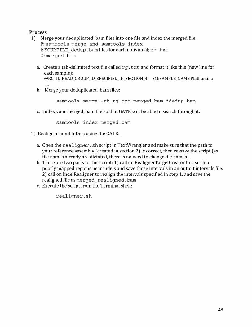
Process

tools  merge and1) Merge am files into one file and  e

samtools index FILE_dedup.bam files for each individual; rg.txt 

 your deduplicated .b index th  merged file.   P: sam

I: YOUR   

O: merged.bam 

 a.   Create a tab‐delimited text file called rg.txt and format it like this (new line forample): 

_SECTION_4     SM:SAMPLE_NAME PL:Illumina each s

  @RG  ID:READ_GROUP_ID_SPECIFIED_IN…. 

rge your deduplicated .bam files:  b.    Me     samtools merge –rh rg.txt merged.bam *dedup.bam c.   Index your merged .bam file so that GATK will be able to search through it:   samtools index merged.

2)  Realign around InDels using 

bam

the GATK. 

a. Open the realigner.sh script in TextWrangler and make sure that the path to s 

your reference assembly (created in section 2) is correct, then re‐save the script (afile names already are dictated, there is no need to change file names). 

b. There are two parts to this script: 1) call on RealignerTargetCreator to search for poorly mapped regions near indels and save those intervals in an output.intervals file. 

vals specified in step 1, and save the  

2) call on IndelRealigner to realign the interrealigned file as merged_realigned.bam

c. Execute the script from the Terminal shell:  realigner.sh

               

48

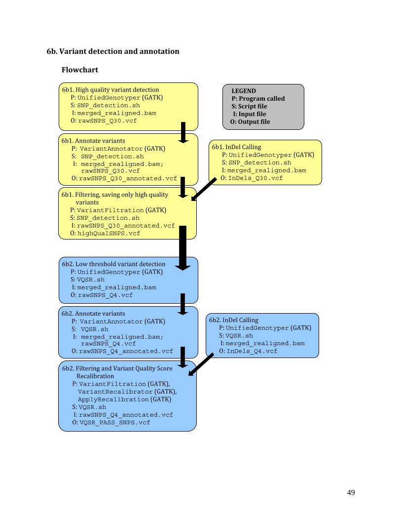
6b. Variant detection and annotation  

6b2. Filtering and Vecalibration 

ariant Quality Score 

VariantFiltration (          R

t ecalibrato ),         P:  GATK),  

r (GATKpplyRecalibration (GATK) 

           Varian R

QSR.sh            A

PS_Q4_annotated.vcf        S: V        I: rawSN       O: VQSR_PASS_SNPS.vcf 

6b1. H t (GATK

NP_detection.s  

igh quality variant de ection UnifiedGenotyper )       P: 

erged_realigned.bam       S: S h       I: m      O: rawSNPS_Q30.vcf 

Flowchart      LEGEND 

    P: Program called      S: Script file       I: Input file    O: Output file 

6b1. An(

SNP_detection.sh 

notate variants        P:  V       S:   

 merged_realigned.bam;

ariantAnnotator  GATK) 

        I:  

 rawSNPS_Q30.vcf

       O: rawSNPS_Q30_annotated.vcf

6b1. F

VariantFiltration (GATK) 

iltering,ariants 

 saving only high quality              v

NP_detection.sh       P: 

S_Q30_annotated.vcf       S: S       I: rawSNP      O: highQualSNPS.vcf 

6b2. L

h 

ow threshold variant detectionUnifiedGenotyper (GATK)       P: 

_realigned.bam       S: VQSR.s       I: merged

f       O: rawSNPS_Q4.vc

6b1. In (

SNP_detection.sh  

Del Calling       P: 

_realigned.bam 

UnifiedGenotyper GATK)  

       S:        I: merged      O: InDels_Q30.vcf 

6b2. An r

VQSR.sh 

notate va iants        P:  V       S:   

 merged_realigned.bam;

ariantAnnotator (GATK) 

        I:          O: rawSNPS_Q4_annotated.vcf 

rawSNPS_Q4.vcf

6b2. In

QSR.sh 

Del Calling       P: 

d_realigned.bam 

UnifiedGenotyper (GATK)         S: V        I: merge       O: InDels_Q4.vcf 

49

Process1)  Detect high quality variant sites. 

Unified Genotyper, VariantAnnotator, VariantFiltration ATK) 

P: 

NP_detection.sh (G

erged_realigned.bam  S: S: m

ualSNPS.vcf IO: highQ 

a.  Open the SNP_detection.sh script in TextWrangler and make sure that the path to your reference assembly (from section 2) is correct (as file names already are dictated, there is no need to change file names). Re‐save the script. The script has six elements: 1) It calls on the Unified Genotyper to confidently call variant sites with a Phred scale quality of more than 30 (probability of being a true variant site >0.999); 2) It calls on VariantAnnotator to add annotations to the .vcf file output from step 1 (for more information, see http://www.broadinstitute.org/gsa/wiki/index.php/VariantAnnotator); 3) It calls on the Unified Genotyper to confidently call indel sites with a Phred scale quality of more than 30; 4) It filters the .vcf file and adds annotations in the filter column of all sites that are close to indels; 5) It applies a number of other quality filters to the .vcf 

 pass the filters; 6) It saves only the variant o a new file called highQualSNPS.vcf 

file and annotates the sites that do nots that have passed all the filters intcu e script from the Terminal: 

siteb.  Exe te th     

SNP_detection.sh

c.  View the bottom 10 lines of the .vcf file with:  tail highQualSNPS.vcf

and familiarize yourself with the format. For each line, the first nine columns contain information about the variant site (location and quality metrics) as well as a filter flag column. Columns 10 and above contain genotype information for each individual in the dataset. More information about the .vcf file format can be found at: http://www.1000genomes.org/wiki/Analysis/vcf4.0 

 2)   w

50

 Lo  threshold variant detection and Variant Quality Score Recalibration (VQSR) a.  Open the VQSR.sh script in TextWrangler and make sure that the path to your 

reference assembly (from section 2) is correct. Re‐save the script. The script has eight elements: 1) It calls on the Unified Genotyper to confidently call variant sites with a Phred scale quality of more than 4; 2) It calls on VariantAnnotator to add annotations to the .vcf file output from step 1; 3) It calls on the Unified Genotyper to confidently call indel sites with a Phred scale quality of more than 4; 4) It filters the .vcf file and adds annotations in the filter column of all sites that are close to indels; 5) It applies a number of other quality filters to the .vcf file and annotates the sites that do not pass the filters; 6) It uses the high quality SNPS found in step 1 above to build a Gaussian mixture model to be able to accurately distinguish true variant sites from false positives; 7) It applies the models and annotates the variant sites that fail 

to pass the filter; 8) It saves only the variant sitenew file called VQSR_PASS_SNPS.vcf 

cute the script from the Terminal by typing: 

s that have passed the VQSR into a 

b.  Exe     VQSR.sh

6c. Genotype extraction and data analysis  rocess ) EP1 

xtract genotypes in variant sites shared by all individuals: 

Extract genotypes of all individuals at all variable sites from the .vcf file into a format useable by Microsoft Excel, using a genotype quality threshold. 

S: g: V

etgenosfromvcf.py I QSR_PASS_SNPS.vcf O: shared_genotypes.txt  

a.      Execute the python script by typing:  getgenosfromvcf.py VQSR_PASS_SNPS.vcf Genotypes.txt rows 20

 The final argument specifies a genotype Phred quality score cutoff of 20 (99% probability of being true). This parameter can be changed according to your needs. The “rows” argument specifies that SNPs will be output in rows, with two columns per individual, one for each allele (specifying “cols” would return the same output, but with SNPs as columns, two columns per SNP). 

b. 

Once the script has finished, we can create a new file containing only the variant sites for which we have genotype information for all individuals (all lines that do not contain any “.”). We will do this using a combination of the unix commands ‘cat’ and grep’: ‘

cat Genotypes.txt | grep -v ’\.’ > genotypes_shared_by_all.txt

 It is often a good idea to focus on the best quality SNPs when working with next‐gen sequence data. However, some analyses do not require data for all individuals at every SNP (as you will see later in the FST outlier section). 

c. genotypes_shared_by_all.txt can now be opened in Microsoft Excel to visualize the genotype data. Although it is not typically practical to work with next‐gen sequencing data using Excel, it can be a useful format to get comfortable with the ata as well as to calculate allele and genotype frequencies. 

 

d 

 ) Principal Components Analysis: 

51

2 

a. eCr

QSR_PASS_SNPS.vcf 

ate the input files fo  the smartpca program. rcf2smartpca.py S: v

I: VO: PREFIX_Indiv, PREFIX_Geno, PREFIX_SNP, par.PREFIX  This script will convert the genotype data from the .vcf file into the proper format for analysis with the program smartpca. This includes four different files: the Indiv file, the Geno file, the SNP file and the parameter or ‘par’ file. Added to the names of all of the output files will be a prefix specified on the command line when the program is run. In rder to focus in on only high‐quality portions of the dataset, this script will only utilize odata from SNPs that have been genotyped in all individuals.  ake sure that you are in the same directory as your files, then execute the script with the ollowing command: Mf vcf2smartpca.py VQSR_PASS_SNPS.vcf passing_snps_q20 20 popfile \

INDIVIDUALS_TO_OMIT n this case, the prefix used is ‘passing_snps_q20.’ This argument can be any arbitrary Istring of characters, but it is nice to try to make it as informative as possible.   The third argument (20) is an integer specifying a minimum genotype quality cutoff. This is a cut‐off for the quality of the individual‐level genotypes, as opposed to the SNP quality as a whole. Individuals with genotype qualities below the minimum threshold will be treated as missing data. Therefore, you should try preparing input files at a couple different quality cut‐offs. Choose a cut‐off that provides a good number of SNPs (1000s, at least), while cutting out some portion of the worst quality genotypes. After creating the input files, the script will print to the screen the number of SNPs that were included in the input files for the smartpca analysis.  popfile should be a plain text file that relates each of your individuals to its population of origin. It should have one line per individual. Each line should contain two strings. The first should be an individual ID (exactly the same as specified in the .vcf file). The second should be the population that individual was sampled from. The two strings can be eparated by any amount of whitespace. The popfile must have an entry for every 

he .vcf file  w). sindividual in t even if some individuals are omitted from the outfiles (see belo Following the popfile argument, you can specify the names of individuals that are in your .vcf file but which you do not want to include in the PCA. These names should be dentical to the names in the .vcf file and should be separated by whitespace. If no names 

 PCA. iare specified then all individuals will be included in the

b. n the princ pal components analysis using smartpca:  

i 

Ru

REFIX_Indiv, PREFIX_Geno, PREFIX_SNP, par.PREFIX P: smartpcaI: PO: PREFIX_#LOCI.eval, PREFIX_#LOCI.eval, PREFIX_snpweights,

52

PREFIX_logfile.txt  Execute the script with the following command:  smartpca –p par.passing_snps_q20 > passing_snps_q20_logfile.txt

There are several runtime parameters that are specified in the ‘par’ file. The above script automatically sets these parameters to levels that we have found to be useful in our data nalysis. However, these parameters can easily be changed prior to running the analysis. 

aAll parameters are described in the help pages for smartpca.  This analysis will generate a number of output files. The one that we are the most interested in is the one with the extension ‘.evec’, This file contains each individual’s loadings on each of the principle components, and it is these loadings that we will plot to visualize the data. Open this eigenvector file in TextWrangler. The top row specifies the amount of variance explained by each of the eigenvectors. This is followed by one row per individual containing that individual’s loadings for each principle component. 

 To easily work with the data in Excel, we need to replace all of the whitespace in the file with tabs. We can do this with a simple find and replace within TextWrangler. To do so, press command + f, search for ‘ +’ (that is a single space character followed by a plus sign) and then replace with ‘\t’ (this is the regular expression for a tab character, make sure that he ‘grep’ box is checked in the ‘find’ dialog box). This search and replace, therefore, will treplace any continuous stretch of spaces with a single tab character.  We can then copy and paste the contents of this file into Excel and create scatterplots to visualize the data. It is best to start by comparing principle components 1 & 2 because these will explain the largest variance in the data. Plot different ‘series’ for each population in the analysis so that differences can be easily visualized. If populations are significantly differentiated then we expect to see clustering of individuals by their respective populations. This clustering will not necessarily occur on the first several principle omponents though, so go ahead and visualize at least the first five or six, to see the major ctrends in the data.  The number of individuals that are included in the analysis determines the number of ossible principal components for a data set. However, the default for this script is to only preport the top 8 (this can be changed in the ‘par’ file).    PCA is most useful for getting a general idea of the major trends in the data set. However, it is also possible to look at the loci that explain the most of the variance in the data along a particular axis (i.e. likely to be under selection). This is done by looking at the PREFIX_snpweights output file. This file contains weights for each SNP along all reported principle component axes. The higher the absolute value of the weight, the stronger the correlation of that SNP with that principle component. Open the snpweight file in TextWrangler, and replace all white space with tabs (as above). Then copy and paste 

53

the data into Excel and find the most strongly weighted SNPs for the first few principal components. 

c. e

  ntify the number of significant eigenvectors using twstats: Id

refix_#loci.eval P: twstatsI: pO: prefix_twstats.txt  twstats is a second program that comes in the Eigensoft package. It takes the ‘.eval’ file output during the smartpca analysis and calculates the significance of each principal component. This is a useful tool for determining the number of principal components exhibiting meaningful variation. However, the Tracy‐Widom statistics used to determine ignificance can break down under certain conditions. See Patterson et al. (2006) for more sdetails.  Execute the script with the following command: 

twstats –t twtable –I passing_snps_q20_#loci.eval \ –o passing_snps_q20_twstats.txt

twtable is necessary for these calculations. It is distributed along with the Eigensoft package and should be located in your programs folder. 

3) FST Outliers:  A targeted approach to look for patterns of local selection is to look for FST outliers. This approach compares the level of differentiation at a given locus to levels of differentiation across the genome (or transcriptome) to determine whether there is evidence of selection. For example, a locus that is significantly more divergent than average has likely been affected by positive or directional selection. Similarly, lower than usual FST suggests either balancing or purifying selection. To conduct an FST outlier analysis we will use the program BayeScan, which uses a Bayesian framework to estimate the probability that each locus has been acted on y b  selection 

 a. eate input for BayeScan: Cr

QSR_PASS_SNPS.vcf S: make_bayescan_input.pyI: V

O: bayes_input.txt, snpkey.txt  As input, BayeScan requires allele frequency counts for each SNP in each population. To generate this input file we will use the script make_bayescan_input.py. This script extracts allele count data from a .vcf file. Because this analysis does not require individual level data, it is less critical to limit the analysis to SNPs with full coverage across all individuals. Therefore, by default this script will include any SNP that has high quality genotype information from at least 5 individuals in each population (the number of 

54

individuals required per population can be changed with an optional third argument on he command line). This allows us to increase the minimum genotype quality score while tstill maintaining a large number of SNPs.  Execute the script with the following command:  make_bayescan_input.py VQSR_PASS_SNPs.vcf popfile 20 [# indivs req/pop] popfile should be a plain text file that relates each of your individuals to its population of origin. It should have one line per individual. Each line should contain two strings. The first should be an individual ID (exactly the same as specified in the .vcf file). The second should be the population that individual was sampled from. The two strings can be separated by any amount of whitespace. The popfile does not need to have an entry for very individual in the .vcf file. Therefore, this script can be used to pull out information efrom subsets of your data set.  The third argument on the command line (and the last required argument) is an integer specifying the minimum genotype quality for a SNP to be used in the analysis. Depending on the size of the .vcf file this process may take several minutes. This step will generate two files: 1) bayes_input.txt will include the information needed by BayeScan to conduct the analysis and 2) snpkey.txt, which is a reference for you to move from the SNP numbers used by BayeScan to the contig and base pair location of the SNP in the reference contigs. This script will also print to your Terminal window the names of your populations along with the number that each one was given in the input file for BayeScan. o ahead and open these 2 files in Textwrangler to get an idea of their formats. Also, 

quality criteria. Gcheck the number of SNPs that met the specified 

b. n the analysis for FST 

 outliers using BayeScan: ayes_input.txt 

RuI: bO: bayes_input_fst.txt, bayes_input.sel, bayes_input_AccRte.txt, bayes_input_Verif.txt P: BayeScan  Execute the program with the following command: 

BayeScan2.0_macos64bits bayes_input.txt

he first argument on the command line is the executable program. The exact name may Tvary depending on your operating system and version.  This analysis will likely take several hours to complete. When it is done it will have created several output files. The main file of interest is bayes_input_fst.txt. One way to visualize the results is to use a function in R that is included with the BayeScan istribution. It is distributed in the script plot_R.r. To load this function into R, open he R console and type the following command: dt 

source (“path/to/plot_R.r”)

55

56

Then, run the function on the BayeScan results using the following command: 

plot_bayescan(“path/to/bayes_input_fst.txt”, FDR=0.05) This function will calculate the Posterior Odds (PO) threshold leading to a false discovery ate of no more that 5%. Using the posterior odds value it will find and list the SNPs that rare FST outliers. It will also produce a figure of FST vs. log(PO).  Additionally, you can look at what SNPs are nearly significant by opening the file bayes_input_fst.txt in Excel and sorting based on the second column, which corresponds to the probability that a SNP has been affected by selection. The largest values indicate the SNPs that are most likely to have been affected by selection.  

 Summary Within this section, we have processed our alignment files from section 4 and created a transcriptome‐wide list of variant sites that we are confident in. From this list, we have extracted the variant sites for which we could confidently assign genotypes to all individuals in our dataset, both in a format that we could input into Excel and a format that we could input into a principal components analysis. For an FST outlier analysis, we extracted a somewhat larger dataset of all variant sites for which there were confident genotypes for at least 5 individuals per population.