Simple computer code for estimating cosmic-ray shieldingby oddly shaped objects

Greg Balcoa,∗

a Berkeley Geochronology Center, 2455 Ridge Road, Berkeley CA 94709 USA

Abstract

This paper describes computer code that estimates the effect on cosmogenic-nuclideproduction rates of arbitrarily shaped obstructions that are partially or completely opaqueto cosmic rays. This is potentially useful for cosmogenic-nuclide exposure dating ofgeometrically complex landforms. The code has been validated against analytical for-mulae applicable to objects with regular geometries. It has not yet been validatedagainst empirical measurements of cosmogenic-nuclide concentrations in samples withthe same exposure history but different shielding geometries.

Keywords: Cosmogenic nuclide geochemistry, Exposure-age dating, Monte Carlointegration, Precariously balanced rocks

1. Importance of geometric shielding of the cosmic-ray flux to exposure dating 1

Cosmogenic-nuclide exposure dating is a geochemical method used to determine 2

the age of geological events that create or modify the Earth’s surface, such as glacier 3

advances and retreats, landslides, earthquake surface ruptures, or instances of erosion 4

or sediment deposition. To determine the exposure age of a rock surface, one must 5

i) measure the concentration of a trace cosmic-ray-produced nuclide (e.g., 10Be, 26Al, 6

3He, etc.); and ii) use an independently calibrated nuclide production rate to interpret 7

the concentration as an exposure age (see review in Dunai, 2010). 8

Typically (Dunai, 2010), estimating the production rate at a sample site employs 9

simplifying assumptions that i) the sample is located on an infinite flat surface, and ii) 10

any topographic obstructions to the cosmic-ray flux can be represented as an apparent 11

horizon below which cosmic rays are fully obstructed, and above which they are fully 12

admitted. These assumptions are adequate for a very wide range of useful exposure- 13

dating applications, but they fail when the sample site is located on or near objects 14

whose dimensions are similar to the cosmic ray particle attenuation length in rock 15

(order 1 meter). 16

The main reason this assumption fails is referred to in this paper as ‘geometric 17

shielding.’ Geometric shielding describes the effect that when a sample is surrounded 18

∗Corresponding author. Tel. 510.644.9200 Fax 510.644.9201Email address: balcs@bgc.org (Greg Balco )

Preprint submitted to Quaternary Geochronology October 3, 2013

by obstructions, the cosmic-ray flux from certain directions must pass through rock 19

or sediment, rather than only air, before reaching the sample site. If the thickness of 20

rock traversed is long relative to the cosmic-ray attenuation length, then the cosmic-ray 21

flux from that direction is completely attenuated and the opaque-horizon assumption 22

described above is adequate. However, if it is relatively short then the cosmic-ray 23

flux is only partially attenuated and this assumption fails. The term ‘self-shielding’ 24

is sometimes used to describe this effect, although this term is somewhat misleading 25

because both the rock that is being sampled (‘self’) and other nearby objects could both 26

shield the sample site. 27

Another effect that is potentially important for samples not embedded in infinite flat 28

surfaces is here called the ‘missing mass effect;’ Masarik and Wieler (2003) also called 29

this the ‘shape effect.’ This describes the fact that a minority of cosmogenic-nuclide 30

production at or beneath the Earth’s surface is due to secondary particles originating 31

from nuclear reactions within the surrounding rock mass. Given a sample embedded 32

in an infinite flat surface, secondary particles responsible for nuclide production in the 33

sample are produced all around the sample site. However, when a sample location is 34

in part surrounded by air rather than rock – for example if it lies on a steeply dipping 35

surface, or within a relatively small boulder – the flux of these secondary particles, and 36

therefore the production rate, is less. 37

The magnitude of geometric shielding can vary from negligible to complete atten- 38

uation depending on the arrangement and size of obstructions. The magnitude of the 39

missing mass effect is expected to be at most ∼10% of the production rate (i.e., for 40

the extreme case in which a sample lies at the top of a tall, thin pillar; Masarik and 41

Wieler, 2003). Thus, in many common geomorphic situations, geometric shielding is 42

significantly more important (a tens-of-percent-level effect on the production rate) than 43

the missing mass effect (a percent-level effect). Geometric shielding is also easier to 44

calculate. The remainder of this paper describes computer code that computes geo- 45

metric shielding for arbitrary geometry of samples and obstructions; this computation 46

only requires computing the lengths of ray paths that pass through objects and apply- 47

ing an exponential attenuation factor to each ray path. Computer code to implement 48

this is simple and fast enough to permit, for example, dynamic calculation of shielding 49

factors in a model where the shielding geometry evolves during the exposure history 50

of a sample. Previous attempts to quantify the missing mass effect, on the other hand, 51

employed a complete simulation of the cascade of nuclear reactions in the atmosphere 52

and rock that give rise to the particle flux at the sample site, using first-principles par- 53

ticle interaction codes such as MCNP or GEANT (Masarik and Beer, 1999, and ref- 54

erences therein). These codes are slow, complex, and require extensive computational 55

resources. To summarize, because of the difference in the potential magnitude of these 56

two effects, there are many geomorphically relevant situations involving obstructed 57

samples in which one can estimate production rates at useful (i.e., percent-level) ac- 58

curacy using only the relatively simple geometric shielding calculation. The calcula- 59

tions in this paper consider only the geometric shielding effect and do not consider the 60

missing mass effect. A valuable future contribution would be to develop a simplified 61

method of approximating the missing mass effect using only geometric considerations 62

that would not require complex particle physics simulation code. 63

Although both the geometric shielding effect and the missing mass effect follow 64

2

from well-established physical principles, there has been very little attempt to verify 65

calculations of these effects by measuring cosmogenic-nuclide concentrations in natu- 66

ral situations where they are expected to be important. For example, the missing mass 67

effect predicts a relationship between boulder size, sample location on a boulder, and 68

cosmogenic-nuclide concentration. Although some researchers have argued that this 69

relationship is or is not present in certain exposure-age data sets (Masarik and Wieler, 70

2003; Balco and Schaefer, 2006), the scatter in these data sets is similar in magnitude 71

to expected effects, so these results were ambiguous. A more comprehensive example 72

is the study of Kubik and Reuther (2007), who attempted to match cosmogenic 10Be 73

concentrations measured on and beneath a cliff surface, where both geometric shield- 74

ing and missing mass effects would be expected to be important, with model estimates 75

of these effects. However, they were not able to reconcile observations with predictions 76

at high confidence. 77

To summarize, a method of computing cosmogenic-nuclide production rates on, 78

near, and within arbitrarily-shaped objects is potentially useful for exposure-dating ap- 79

plications, because many landforms of geomorphic and geologic interest have complex 80

shapes at the scale of cosmic-ray attenuation lengths. As discussed above and as noted 81

by others including Dunne et al. (1999), Lal and Chen (2005), and Mackey and Lamb 82

(2013), in many cases this can be accomplished at adequate precision by considering 83

only geometric shielding. The computer code described in this paper was originally 84

developed for exposure-dating of precariously balanced rocks used in seismic hazard 85

estimation (Balco et al., 2011). These rocks are gradually exhumed by erosion of sur- 86

rounding soil, and determining the rate and timing of this exhumation requires collect- 87

ing samples on the sides of the rocks at a range of heights. As most of these rocks are 88

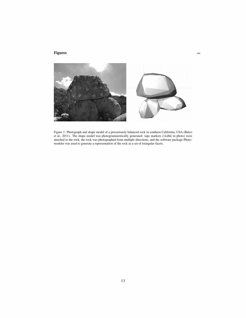
1-2 meters in size and irregular in shape (e.g., Figure 1), these sample locations are 89

subject to partial shielding by the rock itself, and the magnitude of this shielding varies 90

with sample location. In addition, when the rock is partially exhumed, sample sites can 91

also be shielded by soil. To calculate these effects, in Balco et al. (2011) we developed 92

computer code to calculate geometric shielding factors for arbitrarily shaped objects. 93

However, that paper did not include the code or describe it in detail. The present paper 94

provides a complete description and includes the code as supplementary information. 95

For purposes of review of this paper, the MATLAB code, documentation, and 96

ancillary information is available online at: 97

http://noblegas.berkeley.edu/~balcs/shielding_calcs/ 98

99

2. Definition of geometric shielding; previous work 100

The treatment of geometric shielding in this paper follows that of Lal (1991), which 101

was also adopted by Dunne et al. (1999), Lal and Chen (2005), and Mackey and Lamb 102

(2013). Dunne et al. (1999) provides a complete and clear derivation of the following 103

equations. Cosmic ray intensity as a function of direction I(θ, φ), where θ is the zenith 104

angle measured down from the vertical and φ is the azimuthal angle, is assumed to be 105

constant in azimuth but vary with zenith angle, such that: 106

3

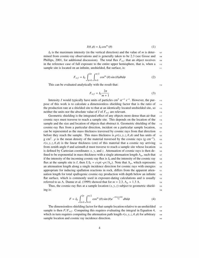
I(θ, φ) = I0 cosm (θ) (1)

I0 is the maximum intensity (in the vertical direction) and the value of m is deter- 107

mined from cosmic-ray observations and is generally taken to be 2.3 (see Gosse and 108

Phillips, 2001, for additional discussion). The total flux Fre f that an object receives 109

in the reference case of full exposure to the entire upper hemisphere, that is, when a 110

sample site is located on an infinite, unshielded, flat surface, is: 111

Fre f = I0

∫ 2π

φ=0

∫ π/2

θ=0cosm (θ) sin (θ)dθdφ (2)

This can be evaluated analytically with the result that: 112

Fre f = I02π

m + 1(3)

Intensity I would typically have units of particles cm2 sr−1 s−1. However, the pur- 113

pose of this work is to calculate a dimensionless shielding factor that is the ratio of 114

the production rate at a shielded site to that at an identically located unshielded site, so 115

neither the units nor the absolute value of I of Fre f are relevant. 116

Geometric shielding is the integrated effect of any objects more dense than air that 117

cosmic rays must traverse to reach a sample site. This depends on the location of the 118

sample and the size and location of objects that obstruct it. Geometric shielding of the 119

cosmic-ray flux from a particular direction, incident on a particular sample location, 120

can be represented as the mass thickness traversed by cosmic rays from that direction 121

before they reach the sample. This mass thickness is ρr(x, y, z, θ, φ) and has units of 122

g cm2. ρ is the mean density of the material traversed by the cosmic rays (g cm−3). 123

r(x, y, z, θ, φ) is the linear thickness (cm) of this material that a cosmic ray arriving 124

from zenith angle θ and azimuth φ must traverse to reach a sample site whose location 125

is defined by Cartesian coordinates x, y, and z. Attenuation of cosmic rays is then de- 126

fined to be exponential in mass thickness with a single attenuation length Λp, such that 127

if the intensity of the incoming cosmic-ray flux is I0 and the intensity of the cosmic ray 128

flux at the sample site is I, then I/I0 = exp(−ρr/Λp). Note that Λp, which represents 129

an attenuation length along a single incidence direction for cosmic rays with energies 130

appropriate for inducing spallation reactions in rock, differs from the apparent atten- 131

uation length for total spallogenic cosmic-ray production with depth below an infinite 132

flat surface, which is commonly used in exposure-dating calculations and is usually 133

referred to as Λ. Dunne et al. (1999) showed that for m = 2.3, Λp ' 1.3 Λ. 134

Thus, the cosmic-ray flux at a sample location (x, y, z) subject to geometric shield- 135

ing is: 136

F = I0

∫ 2π

φ=0

∫ π/2

θ=0cosm (θ) sin (θ)e−

ρr(x,y,z,θ,φ)Λp dθdφ (4)

The dimensionless shielding factor for that sample location relative to an unshielded 137

sample is then F/Fre f . Computing this requires evaluating the integral in Equation 4, 138

which in turn requires computing the attenuation path length r(x, y, z, θ, φ) for arbitrary 139

sample location and cosmic ray incidence direction. 140

4

This approach to computing geometric shielding includes several important sim- 141

plifications, two of which are highlighted here. First, it applies only to high-energy 142

cosmic ray neutrons that interact through spallation reactions. It is not appropriate for 143

describing attenuation of the cosmic-ray muon flux. However, the stopping distance 144

of muons in rock is an order of magnitude or more longer than that for high-energy 145

neutrons, so the effect of meter-scale surface obstructions on production rates due to 146

muons is expected to be negligible. Second, this approach disregards the energy spec- 147

trum of cosmic-ray neutrons by assuming that all cosmic-ray particles inducing spalla- 148

tion reactions display the same attenuation length in rock. In principle, the geometric 149

shielding factor associated with a particular obstruction geometry would be expected 150

to vary somewhat as the cosmic-ray energy spectrum varies with elevation and position 151

in the Earth’s magnetic field. However, I am not aware of any attempts to calculate the 152

magnitude of this variation. 153

Several previous authors have computed shielding factors using the formulae above 154

for regular geometries where attenuation path lengths r can be represented by analytical 155

functions of x, y, z, φ, and θ. Dunne et al. (1999) computed shielding factors at and 156

below flat and dipping surfaces subject to complete obstruction of the cosmic-ray flux 157

from some fraction of the upper hemisphere. Lal and Chen (2005) also computed 158

shielding factors below dipping surfaces, and in addition for the interior of spherical 159

and rectangular boulders. Mackey and Lamb (2013) considered spheres. However, 160

natural rock landforms that one might wish to exposure date are commonly irregularly 161

shaped, which requires a numerical integration method. The method described here 162

uses Monte Carlo integration to evaluate the integral and a ray-tracing method, applied 163

to a representation of the shielding objects as a set of triangular facets, to compute the 164

path lengths. This approach is similar to that used by Plug et al. (2007) to compute 165

the cosmic-ray shielding effect of a forest. The overall goal of this paper is to provide 166

simple publicly available computer code implementing the Monte Carlo integration 167

that can be applied to an arbitrary shielding geometry defined by a commonly used file 168

format. 169

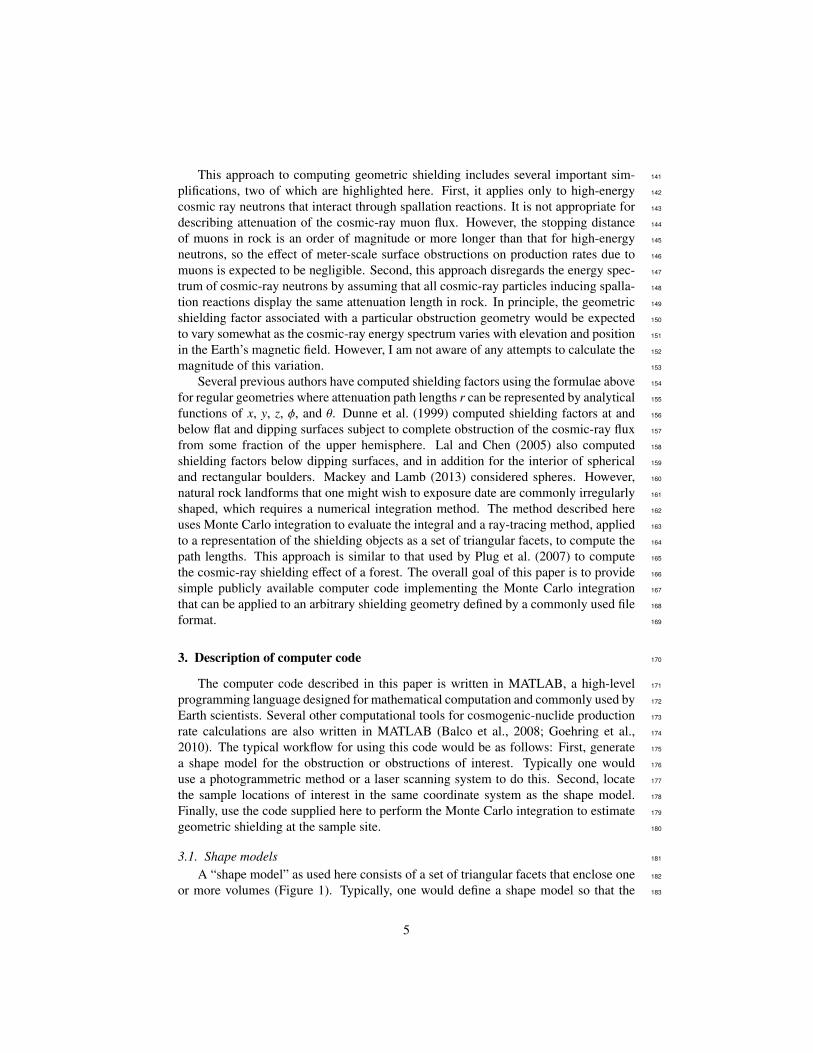
3. Description of computer code 170

The computer code described in this paper is written in MATLAB, a high-level 171

programming language designed for mathematical computation and commonly used by 172

Earth scientists. Several other computational tools for cosmogenic-nuclide production 173

rate calculations are also written in MATLAB (Balco et al., 2008; Goehring et al., 174

2010). The typical workflow for using this code would be as follows: First, generate 175

a shape model for the obstruction or obstructions of interest. Typically one would 176

use a photogrammetric method or a laser scanning system to do this. Second, locate 177

the sample locations of interest in the same coordinate system as the shape model. 178

Finally, use the code supplied here to perform the Monte Carlo integration to estimate 179

geometric shielding at the sample site. 180

3.1. Shape models 181

A “shape model” as used here consists of a set of triangular facets that enclose one 182

or more volumes (Figure 1). Typically, one would define a shape model so that the 183

5

facets form a closed irregular polyhedron for each obstruction. However, one could 184

also define a set of facets that did not form a closed volume, for example to represent a 185

cliff face or hillside. 186

This code reads in shape files defined in the ASCII .stl file format 1. “STL” stands 187

for “standard tesselation language.” This file format is commonly used in 3-D modeling 188

software, 3-D printing, and computer-aided design and manufacturing. The file begins 189

with a line defining the name of the solid, and is followed by a series of line groups, 190

each of which defines the vertices of a triangular facet. An example of a .stl file defining 191

two facets is as follows: 192

solid [C:\Users\balcs\Documents\temp.stl] 193

facet normal 0.00 0.00 0.00 194

outer loop 195

vertex -4.957786 -2.770371 0.602929 196

vertex -4.896107 -2.830239 0.808729 197

vertex -4.975159 -2.737364 0.196783 198

endloop 199

endfacet 200

facet normal 0.00 0.00 0.00 201

outer loop 202

vertex -5.194063 -3.575649 -0.017283 203

vertex -5.434190 -3.412690 -0.130366 204

vertex -5.042836 -3.470916 -0.059296 205

endloop 206

endfacet 207

endsolid 208

Each line beginning with ‘vertex’ contains the x, y, and z coordinates of one of the 209

vertices of the facet. In general, a .stl file contains no scale information and the units are 210

arbitrary. This code assumes that the coordinates of the vertices have units of meters. 211

The three values in each line beginning with ‘facet normal’ are intended to define the 212

unit normal vector of each facet. However, as this information is redundant with the 213

coordinates of the vertices, many software packages dealing with .stl files (including 214

this one) ignore values in these positions or insert zeros. In some implementations of 215

.stl files, the order of the vertices indicates ‘inside’ and ‘outside’ sides of each facet, 216

i.e., the vertices are defined in clockwise order when viewed from the outside of the 217

object. The order of the vertices is ignored here. A binary version of the .stl file format 218

exists, but is not supported here. 219

In previous work (Balco et al., 2011) we used the photogrammetric software Pho- 220

tomodeler (www.photomodeler.com) to generate .stl files describing precariously bal- 221

anced boulders that were the subject of an exposure-dating study. Figure 1 shows an 222

example. 223

1e.g., http://en.wikipedia.org/wiki/STL (file format)

6

3.2. Path length calculation 224

The result of reading a shape model into the MATLAB code is a number of sets 225

of three [x, y, z] triples, each set defining a facet. Given this information and the co- 226

ordinates of a sample location in the same coordinate system, the thickness of rock 227

traversed by a cosmic ray with arbitrary direction is calculated using the following 228

algorithm. 229

1. Change coordinates. Shift the coordinates of the shape model and sample lo- 230

cation so that the sample location is at coordinates [0, 0, 0]. That is, if a vertex 231

as originally defined in the shape model has coordinates [a, b, c] and the sample 232

location as originally defined has coordinates [as, bs, cs], transform them to new 233

coordinates [x, y, z] where x = a − as, y = b − bs, and z = c − cs. Basically, the 234

effect of this transformation is to represent each vertex in the shape model as a 235

vector originating at the sample site. 236

2. Check for intersections between a cosmic ray and each facet in the shape model. 237

The means of doing this relies on the fact that in the sample-centered coordinate 238

system, the vector representing a cosmic ray incident on the sample location is a 239

linear combination of the vectors representing the corners of a facet. If the vector 240

representing a cosmic ray incidence direction has coordinates xr, yr, and zr, and 241

the three vertices of the facet have coordinates xi, yi, and zi where i = 1...3, then: 242x1 y1 z1x2 y2 z2x3 y3 z3

pqr

=

xr

yr

zr

(5)

This is useful because if p, q, and r are all greater than zero, then the cosmic ray 243

passes through the facet. Thus, solving Equation 5 for each facet enables one to 244

identify those facets that the ray passes through. Figure 2 shows an example. In 245

principle this is computationally inefficient because one must consider all facets 246

for each cosmic ray. However, it is fast enough for this purpose. 247

3. Calculate the path distances in rock. Having identified the facets in the shape 248

model that the ray passes through, one can compute i) the points of intersection 249

between the ray and each facet, and ii) the distance between each intersection 250

point and the sample location. If there are a large number of objects in the 251

shape model, then there could be many such intersection points. This requires 252

some way of determining which sections of the ray path are inside objects and 253

which are outside. The algorithm to accomplish this involves assuming that the 254

sample location is within an object. In reality, this should always the case for an 255

exposure-dating application because the sample collected for analysis has some 256

thickness greater than zero, and the production rate calculation applies to the 257

shape of the object before the sample was removed. Thus, the center of the 258

sample where one wishes to compute the production rate is, by definition, inside 259

an object. In the simplest case where the shape model contains a single convex 260

object, then any cosmic ray can only intersect one facet, where it enters the object 261

on its way to the sample location. In a more complicated case including a single 262

non-convex object or many objects, then the ray can enter or exit many different 263

objects, or the same object multiple times, intersecting 2n + 1 facets where n 264

7

is the number of additional objects intersected (or the number of crossings of 265

one complex object). Thus, one can determine which sections of the ray path 266

lie within rock by sorting the intersection points according to distance from the 267

sample location and assuming that the pathlength between the sample and the 268

closest intersection is rock, the pathlength between the closest and second-closest 269

intersections is air, the pathlength between the second-closest and third-closest 270

intersections is rock, and so on. See Figure 2. Note that this algorithm assumes 271

that all objects are closed shapes, which implies that there will always be an 272

odd number of intersections. An even number of intersections could only arise 273

from a topological error in defining the objects in the shape model. However, 274

in practice it might be potentially useful to define some non-closed shapes in a 275

shape model to represent objects that are large enough to fully stop the cosmic- 276

ray flux, e.g., cliff faces or hillsides. To accommodate this, the code provides an 277

option to assume that an even number of intersections signals total attenuation 278

of a particular cosmic ray. 279

In applying this method to exposure dating of precariously balanced rocks in Balco 280

et al. (2011), we also allowed for the possibility that objects were embedded in soil 281

whose surface lay above the sample site. This can be accounted for by computing 282

the intersection between the cosmic ray and a horizontal soil surface, disregarding all 283

cosmic ray-facet intersections that lie below the soil surface, and applying the algo- 284

rithm in (3) above to the intersection with the soil surface and any remaining ray-facet 285

intersections. 286

3.3. Monte Carlo integration 287

The algorithm described above applied to a shape model enables one to compute 288

r(x, y, z, θ, φ), the thickness of rock that a cosmic ray with arbitrary zenith angle θ and 289

azimuth φmust traverse to reach a sample at arbitrary coordinates [x, y, z]. This permits 290

numerical integration of Equation 4 by Monte Carlo integration. Monte Carlo integra- 291

tion is a method of estimating the integral of a function over some region by generating 292

a uniformly distributed random sample of points within the region and computing the 293

value of the function at those points. In general, given a function of two variables x 294

and y to be integrated over a region 0 ≤ x ≤ a and 0 ≤ y ≤ b, 295

IMC =abN

N∑i=1

f (xi, yi) '∫ b

0

∫ a

0f (x, y) dx dy (6)

where IMC is the Monte Carlo estimate of the integral, N is the number of points 296

in the sample, and the sample points are uniformly distributed in x and y and have 297

coordinates (xi, yi). Thus, the Monte Carlo estimate for the geometric shielding factor 298

F/Fre f for a sample with coordinates (x, y, z) is: 299(2π

m + 1

)−1π2

N

N∑i=1

cosm (θi) sin (θi)e−ρr(x,y,z,θi ,φi )

Λp (7)

for N sample points (θi, φi) that are uniformly distributed in φ and θ. 300

8

The number of sample points needed for an accurate Monte Carlo estimate of the 301

geometric shielding factor depends on the geometry. One can informally estimate the 302

required sample size by successively increasing the number of sample points and de- 303

termining when the resulting shielding factor converges on a stable and reproducible 304

value. Figure 3 shows an example. In the application to precariously balanced rocks, 305

we found that N ' 500 was nearly always sufficient. 306

3.4. Validation against analytical results 307

I attempted to validate this code by comparing it to analytical formulae, computed 308

by other authors, for the integral in Equation 4 applied to simple geometries. First, 309

Lal and Chen (2005) derived formulae for computing the geometric shielding factor at 310

points within spherical boulders. In this situation, cosmic rays from most directions 311

are partially attenuated by passing through the boulder itself. Figure 4 shows that the 312

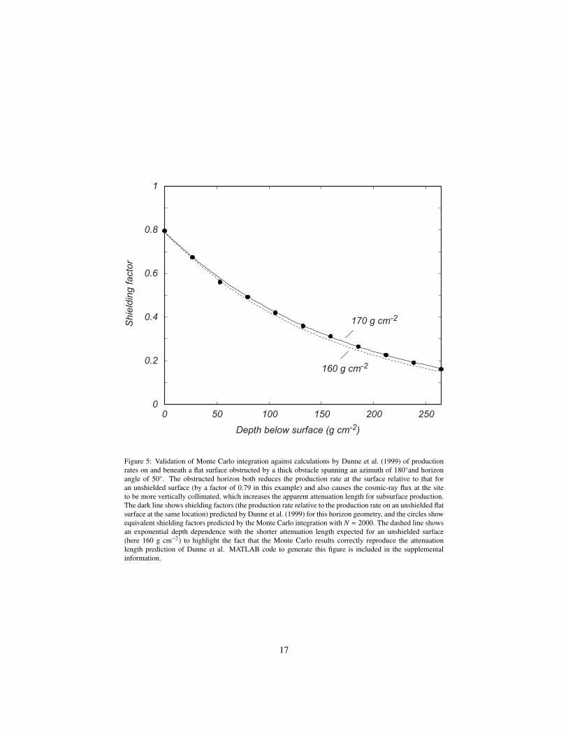
Monte Carlo integration yields the same results as their formulae. Second, Dunne 313

et al. (1999) derived formulas for computing shielding due to complete obstruction of 314

portions of the cosmic-ray flux from part of the upper hemisphere. This case differs 315

from the ones considered by Lal and Chen (2005) and Balco et al. (2011) because it 316

does not involve partial attenuation of the cosmic-ray flux from certain directions, only 317

total obstruction. However, the results of Dunne and others are a useful test of this code 318

because they describe not only a shielding factor at the surface due to an obstructed 319

horizon, but also the effect that the cosmic-ray flux is more vertically collimated when 320

the horizon is obstructed than when it is not, so the depth-dependence of the production 321

rate varies between these cases. The Monte Carlo integration can be used to simulate 322

this effect, and Figure 5 shows that it correctly reproduces the Dunne et al. results. 323

3.5. Validation against measurements 324

In principle, one could validate shielding factors estimated with this code by com- 325

paring them to measured cosmogenic-nuclide concentrations in natural samples. This 326

would require i) an irregularly shaped object with dimensions on the order of 1 m that 327

was emplaced with zero concentration of cosmic-ray-produced nuclides and subse- 328

quently exposed to the cosmic-ray flux without any change in its geometry, ii) a shape 329

model of the object, and iii) measurements of nuclide concentrations from multiple lo- 330

cations on that object that have different degrees of geometric shielding. In this case the 331

cosmogenic-nuclide concentrations will be directly proportional to the true shielding 332

factors, allowing straightforward validation of shielding factor estimates. These con- 333

ditions could be satisfied, for example, by sampling several locations on and/or within 334

a glacially transported moraine boulder. However, because nearly all exposure-dating 335

studies seek to avoid complicated geometric shielding calculations by sampling only 336

from the top of boulders or outcrops, I am not aware of any such data set. 337

10Be measurements on precariously balanced rocks by Balco et al. (2011) and other 338

more recent research (e.g., Rood et al., 2012) collected data that approaches these re- 339

quirements. These data include photogrammetric shape models of irregularly shaped 340

rocks with meter-scale dimensions, and multiple 10Be measurements at different loca- 341

tions on these rocks. However, it is not straightforward to use these data to evaluate the 342

accuracy of shielding factor calculations because the rocks were exhumed by down- 343

wasting of regolith (and the exhumation history is not known independently of the 344

9

10Be measurements), so all the samples did not have the same exposure history, and 345

the shielding geometry changed through time. However, these studies were able to 346

closely match measured 10Be concentrations with a model for 10Be production during 347

rock exhumation that was based on shielding factors computed using the Monte Carlo 348

integration code described here. Figure 6 shows an example discussed by Rood et al. 349

(2012). Calculated shielding factors for samples from this rock vary by a factor of four 350

(from 0.2 to 0.8), and, as shown in Figure 6, variations in measured 10Be concentra- 351

tions have similar pattern and magnitude. Thus, one can find a best-fitting exhumation 352

history (using the method of Balco et al., 2011) that matches measured concentrations. 353

Because the forward model includes many additional assumptions besides the shield- 354

ing factor estimates, this comparison does not directly validate the shielding factor 355

estimates. However, given the large variation in shielding factor among these samples, 356

it would be difficult to match measured nuclide concentrations if the shielding factor 357

estimates were highly inaccurate. Again, a better approach to this would be to make 358

similar measurements on a boulder with a simpler exposure history. This would be a 359

valuable future contribution. 360

4. Example uses 361

The general purpose of the Monte Carlo integration code is to facilitate accurate 362

exposure-dating of samples that are surrounded by meter-scale surface obstructions. 363

In many common exposure-dating situations, for example exposure-dating of glacially 364

transported boulders, complex shielding calculations of this sort are, of course, not 365

necessary because it is easier to select unshielded sample sites. The reason this code 366

was developed for the specific example of estimating exhumation histories for precar- 367

iously balanced rocks useful in seismic hazard analysis is because sampling only un- 368

shielded parts of these features did not provide enough information to reconstruct the 369

exhumation histories responsible for forming them. The fact that the shielding geome- 370

try changes as the rocks are exhumed required a relatively simple and quick method of 371

estimating not only present geometric shielding factors but also changes in the shield- 372

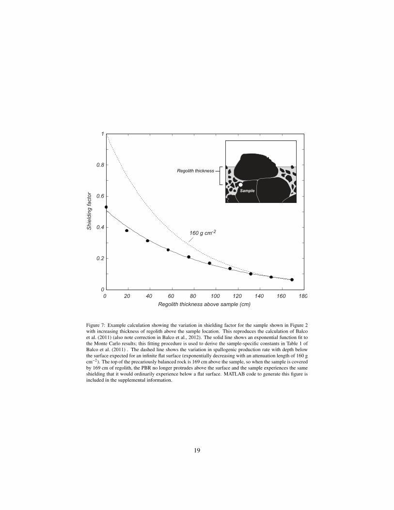
ing factor over time. Figure 7 shows an example calculation for this application, and 373

MATLAB code to generate these results is included in the supplemental material. 374

Other obvious applications include estimating erosion rates where soil erosion leads 375

to progressive exposure of rock features such as tors (e.g., Heimsath et al., 2000), or 376

to estimate when features like arches or sea stacks were formed by cliff retreat. More 377

complex applications would include attempting to determine the frequency of boul- 378

der transport by comparing measured cosmogenic-nuclide concentrations to present 379

shielding geometries (Mackey and Lamb, 2013); or, potentially, archeological applica- 380

tions aimed at verifying that sculpture or stonework has resided in its present geometric 381

configuration since constructed. 382

5. Acknowledgements. 383

Dylan Rood provided the impetus for this work by telling me about precariously 384

balanced rocks in the first place. This work was supported in part by the Ann and 385

Gordon Getty Foundation. 386

10

Balco, G., Purvance, M., Rood, D., 2011. Exposure dating of precariously balanced 387

rocks. Quaternary Geochronology 6, 295–303. 388

Balco, G., Purvance, M., Rood, D., 2012. Corrigendum to “Exposure dating of precar- 389

iously balanced rocks” [Quaternary Geochronology 6(2011) 295-303]. Quaternary 390

Geochronology 9, 86. 391

Balco, G., Schaefer, J., 2006. Cosmogenic-nuclide and varve chronologies for the 392

deglaciation of southern New England. Quaternary Geochronology 1, 15–28. 393

Balco, G., Stone, J., Lifton, N., Dunai, T., 2008. A complete and easily accessible 394

means of calculating surface exposure ages or erosion rates from 10Be and 26Al mea- 395

surements. Quaternary Geochronology 3, 174–195. 396

Dunai, T., 2010. Cosmogenic Nuclides: Principles, Concepts, and Applications in the 397

Earth Surface Sciences. Cambridge University Press: Cambridge, UK. 398

Dunne, J., Elmore, D., Muzikar, P., 1999. Scaling factors for the rates of production 399

of cosmogenic nuclides for geometric shielding and attenuation at depth on sloped 400

surfaces. Geomorphology 27, 3–12. 401

Goehring, B., Kurz, M., Balco, G., Schaefer, J., Licciardi, J., Lifton, N., 2010. A reeval- 402

uation of in-situ cosmogenic He-3 production rates. Quaternary Geochronology 5, 403

410–418. 404

Gosse, J. C., Phillips, F. M., 2001. Terrestrial in situ cosmogenic nuclides: theory and 405

application. Quaternary Science Reviews 20, 1475–1560. 406

Heimsath, A., Chappell, J., Dietrich, W., Nishiizumi, K., Finkel, R., 2000. Soil produc- 407

tion on a retreating escarpment in southeastern Australia. Geology 28 (9), 787–790. 408

Kubik, P., Reuther, A., 2007. Attenuation of cosmogenic 10Be production in the first 409

20 cm below a rock surface. Nuclear Instruments and Methods in Physics Research 410

B 259, 616–624. 411

Lal, D., 1991. Cosmic ray labeling of erosion surfaces: in situ nuclide production rates 412

and erosion models. Earth Planet. Sci. Lett. 104, 424–439. 413

Lal, D., Chen, J., 2005. Cosmic ray labeling of erosion surfaces II: Special cases of 414

exposure histories of boulders, soil, and beach terraces. Earth and Planetary Science 415

Letters 236, 797–813. 416

Mackey, B., Lamb, M., 2013. Deciphering boulder mobility and erosion from cosmo- 417

genic nuclide exposure dating. Journal of Geophysical Research - Earth Surface 118, 418

184–197. 419

Masarik, J., Beer, J., 1999. Simulation of particle fluxes and cosmogenic nuclide pro- 420

duction in Earth’s atmosphere. Journal of Geophysical Research 104, 12099–12111. 421

Masarik, J., Wieler, R., 2003. Production rates of cosmogenic nuclides in boulders. 422

Earth and Planetary Science Letters 216, 201–208. 423

11

Plug, L., Gosse, J., McIntosh, J., Bigley, R., 2007. Attenuation of cosmic ray flux in 424

temperate forest. Journal of Geophysical Research 112, F02022. 425

Rood, D., Anooshehpoor, R., Balco, G., Biasi, G., Brune, J., Brune, R., Grant Ludwig, 426

L., Kendrick, K., Purvance, M., Saleeby, I., 2012. Testing seismic hazard models 427

with be-10 exposure ages for precariously balanced rocks. American Geophysical 428

Union 2012 Fall Meeting, San Francisco, CA. Abstract 1493571. 429

12

Figures 430

Figure 1: Photograph and shape model of a precariously balanced rock in southern California, USA (Balcoet al., 2011). The shape model was photogrammetrically generated: tape markers (visible in photo) wereattached to the rock, the rock was photographed from multiple directions, and the software package Photo-modeler was used to generate a representation of the rock as a set of triangular facets.

13

Figure 2: Intersection of a representative cosmic ray path with the shape model shown in Figure 1. The shapemodel is shown as a wireframe mesh. A near-vertical cosmic ray path to a sample location on the pedestalbelow the precariously balanced rock enters the top of the rock, exits the bottom of the rock, and enters thepedestal to reach the sample location. Facets that intersect the ray path are highlighted by gray fill. Theportion of the cosmic ray path that traverses rock is highlighted by a thickened line.

14

0 200 400 600 800 1000

0

0.2

0.4

0.6

0.8

1

Number of samples

Sh

ield

ing

fa

cto

r

Figure 3: Example of convergence of the Monte Carlo integration estimate of the shielding factor (for thesample location shown in Figure 2) as the sample size increases. Typically the shielding factor converges ona stable value after ∼ 500 iterations.

15

0 0.5 1 1.50

0.2

0.4

0.6

0.8

1

R = 1.5 m

Distance from center of sphere (m)

Sh

ield

ing

fa

cto

r

Along vertical radius

Along horizontal radius

Figure 4: Validation of Monte Carlo integration code against analytical formulae of Lal and Chen (2005) forgeometric shielding factors inside a hemispherical boulder with radius 1.5 meters. The solid and dashed linesare analytical results for samples along vertically-oriented and horizontally-oriented, respectively, radii, andin part reproduce Figure 4 of Lal and Chen (2005). The circles show shielding factors at the same locationscalculated by the Monte Carlo integration with N = 1000. MATLAB code to generate this figure is includedin the supplemental information.

16

0 50 100 150 200 2500

0.2

0.4

0.6

0.8

1

Sh

ield

ing

fa

cto

r

Depth below surface (g cm-2)

160 g cm-2

170 g cm-2

Figure 5: Validation of Monte Carlo integration against calculations by Dunne et al. (1999) of productionrates on and beneath a flat surface obstructed by a thick obstacle spanning an azimuth of 180°and horizonangle of 50°. The obstructed horizon both reduces the production rate at the surface relative to that foran unshielded surface (by a factor of 0.79 in this example) and also causes the cosmic-ray flux at the siteto be more vertically collimated, which increases the apparent attenuation length for subsurface production.The dark line shows shielding factors (the production rate relative to the production rate on an unshielded flatsurface at the same location) predicted by Dunne et al. (1999) for this horizon geometry, and the circles showequivalent shielding factors predicted by the Monte Carlo integration with N = 2000. The dashed line showsan exponential depth dependence with the shorter attenuation length expected for an unshielded surface(here 160 g cm−2) to highlight the fact that the Monte Carlo results correctly reproduce the attenuationlength prediction of Dunne et al. MATLAB code to generate this figure is included in the supplementalinformation.

17

0 50 100

[Be−10] (katoms/g)

2.5

3

3.5

4

4.5

5

He

igh

t (m

, a

rbitra

ry 0

)

Observed

Predicted by best-fit

exhumation history

0 0.80.60.40.2 1

Shielding factor

Figure 6: The right-hand panel shows a shape model for a precariously balanced rock near Lake Los Angeles,CA, described by Rood et al. (2012). Black circles show sample locations. The center panel shows geometricshielding factors calculated by Monte Carlo integration for these samples. The left panel shows cosmogenic10Be concentrations measured by Rood et al. (2012) in these samples (black circles) as well as 10Be concen-trations predicted by a forward model based on these shielding factors and a best-fitting exhumation history(using the method of Balco et al. (2011)) (open circles).

18

0 20 40 60 80 100 120 140 160 180

0

0.2

0.4

0.6

0.8

1

Regolith thickness above sample (cm)

Sh

ield

ing

fa

cto

r

160 g cm-2

Sample

Regolith thickness

Figure 7: Example calculation showing the variation in shielding factor for the sample shown in Figure 2with increasing thickness of regolith above the sample location. This reproduces the calculation of Balcoet al. (2011) (also note correction in Balco et al., 2012). The solid line shows an exponential function fit tothe Monte Carlo results; this fitting procedure is used to derive the sample-specific constants in Table 1 ofBalco et al. (2011) . The dashed line shows the variation in spallogenic production rate with depth belowthe surface expected for an infinite flat surface (exponentially decreasing with an attenuation length of 160 gcm−2). The top of the precariously balanced rock is 169 cm above the sample, so when the sample is coveredby 169 cm of regolith, the PBR no longer protrudes above the surface and the sample experiences the sameshielding that it would ordinarily experience below a flat surface. MATLAB code to generate this figure isincluded in the supplemental information.

19