Similarity Searching for Multi-attribute Sequences · PDF fileSimilarity Searching for...

Similarity Searching for Multi-attribute Sequences�

Tamer Kahveci Ambuj Singh Aliekber G¨urelDepartment of Computer Science Department of Mathematics

University of California, Santa Barbara, CA 93106ftamer,[email protected], [email protected]

Abstract

We investigate the problem of searching similar multi-attribute time sequences. Such sequences arise naturallyin a number of medical, financial, video, weather forecast,and stock market databases where more than one attributeis of interest at a time instant. We first solve the simple casein which the distance is defined as the Euclidean distance.Later, we extend it to shift and scale invariance. We for-mulate a new symmetric scale and shift invariant notion ofdistance for such sequences. We also propose a new indexstructure that transforms the data sequences and clustersthem according to their shiftings and scalings. This clus-tering improves the efficiency considerably. According toour experiments with real and synthetic datasets, the indexstructure's performance is 5 to 45 times better than compet-ing techniques, the exact speedup based on other optimiza-tions such as caching and replication.

1 Introduction

Time series or sequence data sets arise naturally in manyreal world applications like stock market, weather fore-casts, video databases, sensor-based controls, and medicine.There is a frequent need to understand the information con-tent of this data in order to respond better to common trends,to provide corrective emergency steps, or to predict thefuture evolution based on past records. Some examplesof queries on such datasets include finding the companieswhich have similar profit/loss patterns, finding similar mo-tion patterns in a video database, finding similar patterns inmedical sensor data in order to respond to patient healthproblems, to predict infrastructure usage by comparisonwith past trends, or to predict common genetic functionalityby study of gene expression patterns over time.

Time series data is said to haved attributes ifd valuesare stored for each time point. Stock market data, which isformed by storing the closing prices of a company is an ex-ample of a 1-attribute sequence. If we include the P/E ratioand the number of shares sold, this becomes a 3-attributesequence. The trajectory of an object moving on a plane isa 2-attribute sequence, because two values (i.e.X andYcoordinates) are stored for each discrete time point. Med-ical data is usually multi-attribute since a single sensor isseldom sufficient to record the health of a patient: such a

�Work supported partially by NSF under grants EIA-0080134, EIA-9986057, IIS-9877142, ANI-0123985, and NSFIIS98-17432.

sequence can be obtained by using the blood pressure val-ues, the heart beat rate, the amount of calcium, and otherparameters recorded periodically from a patient.

There are many ways to compare the similarity of twotime sequences. One approach is to define the distancebetween two sequences to be the Euclidean distance, byviewing a sequence as a point in an appropriate multi-dimensional space [1, 4, 7, 11, 19].

Range searches and nearest neighbor searches forwholematching and subsequence matching [1] have been theprincipal queries of interest for time series data.Wholematching corresponds to the case when the query sequenceand the sequences in the database have the same length.Agrawal et al. [1] developed one of the first solutions tothis problem. The authors transformed the time sequenceto the frequency domain by using DFT. Later, they reducedthe number of dimensions to a feasible size by storing thefirst few frequency coefficients. Chan and Fu [4] used Haarwavelet transform to reduce the number of dimensions andcompared this method to DFT. The authors found that Haarwavelet transform performs better than DFT. However, theperformance of DFT could be improved using the symme-try of Fourier Transforms [17]. In this case, both methodsgave similar results.

1.1 Adopting new metrics for distance

Non-Euclidean metrics have also been used to computethe similarity for time sequences. Agrawal, Lin, Sawh-ney, and Shim [2] useL1 as the distance metric. An-other distance metric for multi-attribute time sequences isDnorm [13]. Although this metric has a high recall, it al-lows false dismissals.

Defining the distance as some norm of the differencebetween two time sequences may be insufficient if the se-quences can be made closer by linear transformations. Themost important transformations are scaling and shifting.Scaling is needed because of the need to compare time se-quences recorded on devices with different calibrations ordifferent units.

One emerging area of applications for shift and scale in-variant comparison of time sequences is data from genomemicroarrays. By choosing cells from an organism underdifferent stages of development, or under different physi-cal conditions, valuable information can be obtained aboutthe expression of genes, their relationship to one another,and genetic pathways. Using the absolute values of themeasurements may be misleading because of variation inthe physical conditions like data quality and quantity, scan-

1

ner quality, glass quality, hybridization conditions and post-hybridization washing. In order to allow comparisons underdifferent experimental conditions, shift and scale invariantcomparisons of the resulting sequences can be useful.

Das, Gunopulos and Mannila [6] showed that the sim-ilarity between two sequences after eliminating the out-liers, and scaling and shifting can be determined in O(n6)time usinglongest common subsequence (LCSS) technique,wheren is the length of the strings. However, the LCSS canbe found in O((n+m)3�3) time [20] if only shift invarianceis involved, wherem andn are length of sequences and� isthe error.

Rafiei and Mendelzon [16] developed algorithms for an-swering similarity queries under a set of user-specified lin-ear transformations. When these transformations aresafe,the queries can be answered efficiently by applying thespecified transformation to an index MBR. Multiple trans-formations can also be applied collectively to the databasesequences [15]. The problem we study here is different inthat we consider all possible scalings and shiftings, not justa set of user-specified transformations.

Goldin and Kanellakis [8] propose a technique based onnormalization for the comparison of the time sequences.A normalized time sequence has a zero mean and a unitstandard deviation. Given a queryQ, the authors present asearch algorithm that finds all database sequencesS suchthat thenormalized Euclidean distance1 DN (Q; aS+ b) �� for somea > 0 and b. Chu and Wong [5] consideredthe asymmetric formulationD2(aQ + b; S) � �. Theyuse a transformation to map the data sequences onto theShift Eliminated Plane. Both of these formulations of dis-tance are inherently asymmetric in its treatment of queryand database sequences. We focus on the symmetric notionof the distance in this paper. The restriction to only positivescalings (a > 0) also appears artificial.

The Landmark model [14] stores the turning points ofthe time sequences. The distance between time sequenceshere is invariant with respect to 6 transformations: shifting,uniform amplitude scaling, uniform time scaling, uniformbi-scaling, time warping, and non uniform amplitude scal-ing. However, the landmarks of different time sequencesmay correspond to different time points.

1.2 Our contribution

In this paper, we consider the similarity search problemfor multi-attribute sequences. We first solve the simple casein which the distance is basically defined as the Euclideandistance. Later, we extend it to handle shift and scale in-variance. We point out the problems with current meth-ods for scale and shift invariant distance computations, andpropose a new symmetric notion of distance: the distancebetween two time sequences is defined to be the smallestEuclidean distance after scaling and shifting either one ofthe sequences to be as close to the other. We define two

1This corresponds to an unbounded query in the authors' terminology.

models for comparing multi-attribute time sequences: in thefirst model, the scalings and shiftings of the component se-quences are dependent, and in the second model they areindependent.

We propose a novel index structure calledCS-Index(Cone Slice) for shift and scale invariant comparison of timesequences. As a part of this technique, the sequences in thedatabase are first mapped to the shift eliminated plane [5].The transformed points are then clustered in hierarchicalcone slices. These slices are stored on disk according toan in-order traversal, and a pointer to each slice along withangle and spatial extent information is maintained in mem-ory. Given any query, it is first mapped onto shift eliminatedplane. The shift and scale invariant distance between thequery and the slices are computed in memory to obtain aset of candidate slices. The hierarchical construction of theindex structure allows early pruning. Finally, the candidateslices are read from disk in a single seek, and false hits areeliminated.

Experimental results show that the CS-Index structureperforms 50 to 100 times faster than the R*-tree index struc-ture and 5 to 10 times faster than sequential scan. The ef-ficiency of the index structure can be further improved byselectively replicating or caching parts of the index struc-ture.

The rest of the paper is organized as follows. We dis-cuss the simple case in which the Euclidean distance is usedas the dissimilarity measure in Section 2. We define theproblem of shift and scale invariant search of multi-attributetime sequences in Section 3. In Section 4, we propose theCS-index structure for range queries and nearest neighborqueries. We present experimental results on a number ofsynthetic and real datasets in Section 5. We end with a briefdiscussion in Section 6.

2 Multi-attribute time sequencesA d-attribute time sequence is formed by storingd val-

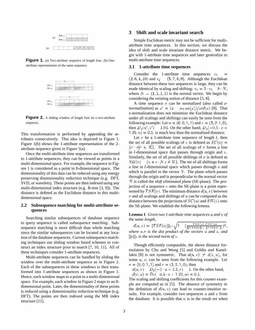
ues at each time point. Ifv is a d-attribute time sequenceof length l, then it can be represented as a vectorv =(v1; v2; :::; vl), wherevi = (vi;1; vi;2; :::; vi;d) for 1 � i � l(vi;j are scalars.). Figure 1(a) depicts a two-attribute se-quence of length four.

The Euclidean distance,D2, betweend-attribute time se-quencesu andv of lengthl is defined as

D2(u; v) =qP

1�i�l

P1�j�d(ui;j � vi;j)2.

2.1 Whole matching for multi-attribute sequences

If the length of the sequences in the database and thelength of the query sequence is equal, similarity searchingis calledwhole matching. Whole matching is a well stud-ied problem for 1-attribute sequences (e.g. [1, 4, 7, 17]).Whole matching problem for multi-attribute sequences canbe solved using any of the existing techniques after trans-forming multi-attribute sequences to 1-attribute sequences.

2

��

��

1Attr

2Attr(a)

��

��

(b)

Figure 1. (a) Two-attribute sequence of length four. (b) One-

attribute representation of the same sequence.

��

��

��

��

1Attr

2Attr

w

��

��

��

��

1Attr

2Attr

w

Figure 2. A sliding window of length four on a two-attribute

sequence.

This transformation is performed by appending the at-tributes consecutively. This idea is depicted in Figure 1.Figure 1(b) shows the 1-attribute representation of the 2-attribute sequence given in Figure 1(a).

Once the multi-attribute time sequences are transformedto 1-attribute sequences, they can be viewed as points in amulti-dimensional space. For example, the sequence in Fig-ure 1 is considered as a point in 8-dimensional space. Thedimensionality of this data can be reduced using any energypreserving dimensionality reduction technique (e.g. DFT,SVD, or wavelets). These points are then indexed using anymulti-dimensional index structure (e.g. R-tree [3, 9]). Thedistance is defined as the Euclidean distance in this multi-dimensional space.

2.2 Subsequence matching for multi-attribute se-quences

Searching similar subsequences of database sequenceto query sequence is calledsubsequence matching. Sub-sequence matching is more difficult than whole matchingsince the similar subsequences can be located at any loca-tion of the database sequences. Current subsequence match-ing techniques use sliding window based schemes to con-struct an index structure prior to search [7, 10, 11]. All ofthese techniques consider 1-attribute sequences.

Multi-attribute sequences can be handled by sliding thewindow over the multi-attribute sequence as in Figure 2.Each of the subsequences in these windows is then trans-formed into 1-attribute sequences as shown in Figure 1.Hence, each window maps to a point in a multi-dimensionalspace. For example, each window in Figure 2 maps to an 8-dimensional point. Later, the dimensionality of these pointsis reduced using a dimensionality reduction technique (e.g.DFT). The points are then indexed using the MR indexstructure [11].

3 Shift and scale invariant search

Simple Euclidean metric may not be sufficient for multi-attribute time sequences. In this section, we discuss theidea of shift and scale invariant distance metric. We be-gin with 1-attribute time sequences and later generalize tomulti-attribute time sequences.

3.1 1-attribute time sequences

Consider the 1-attribute time sequencesv1 =(2; 6; 4; 10) andv2 = (5; 7; 6; 9). Although the Euclideandistance between these two sequences is large, they can bemade identical by scaling and shifting:v1 = 2 � v2 � 8 �N ,whereN = (1; 1; 1; 1) is the normal vector. We begin byconsidering the existing notion of distance [5, 8].

A time sequencex can be normalized (also calledz-normalization) asx0 = (x � mean(x))=std(x) [8]. Thatz-normalization does not minimize the Euclidean distanceunder all scalings and shiftings can easily be seen from thefollowing example: Letu = (0; 0; 1; 1) andv = (3; 2; 1; 0),thenD2(u

0; v0) = 1:94. On the other hand,D2(�0:5 � v +1:25; u) = 0:5: is much less than the normalized distance.

Let v be a 1-attribute time sequence of lengthl, thenthe set of all possible scalings ofv is defined asSC(v) =fc � vjc 2 Rg. The set of all scalings ofv forms a linein l-dimensional space that passes through origin andv.Similarly, the set of all possible shiftings ofv is defined asSH(v) = fv+ c �N jc 2 Rg. The set of all shiftings formsa line in l-dimensional space which passes throughv andwhich is parallel to the vectorN . The plane which passesthrough the origin and is perpendicular to the normal vectorN is called theshift eliminated plane (SE-plane). The pro-jection of a sequencev onto the SE-plane is a point repre-sented byTSE(v). The minimum distanced(u; v) betweenv and all scalings and shiftings ofu can be computed as thedistance between the projections ofSC(u) andSH(v) ontothe SE-plane. We establish the following lemma.

Lemma 1 Given two 1-attribute time sequences u and v ofthe same length,

d(u; v) = jjTSE(v)jj2 �q1� ( TSE(v):TSE(u)

jjTSE(v)jj2�jjTSE(u)jj2)2,

where u:v is the dot product of the vectors u and v, andjjvjj2 is the second norm of v.

Though efficiently computable, the above distance for-mulation by Chu and Wong [5] and Goldin and Kanel-lakis [8] is not symmetric. Thatd(u; v) 6= d(v; u), forsomeu, v, can be seen from the following example. Letu = (0; 0; 1; 1) andv = (3; 2; 1; 0), thend(u; v) = D2(�2 � u+ 2:5; v) = 1. On the other hand,d(v; u) = D2(�0:5 � v + 1:25; u) = 0:5.

The scaling and shifting coefficients for this counter exam-ple are computed as in [5]. The absence of symmetry inthe definition ofd(u; v) can lead to counter-intuitive re-sults. For example, consider two sequencesu andv fromthe database. It is possible thatu is in the result set when

3

we perform a range query usingv as the query sequence, butnot vice-versa. It follows from Lemma 1 that the distancefunctiond(u; v) is symmetric, i.e.d(u; v) = d(v; u), if andonly if jjTSE(u)jj2 = jjTSE(v)jj2. Since this conditionis quite restrictive, we modify the definition of distance inorder to make it symmetric.

Definition 1 Given two 1-attribute time sequences u and vof the same length, the distance between these sequences isdefined asdist(u; v) = minfd(u; v); d(v; u)g.

We could have used other functions such asmax, or av-erage in the above definition, but it is themin function thatcaptures the notion of distance more adequately. We willsee later that our index structure works as well for otherfunctions.

3.2 Multi-attribute time sequences

The attributes of a multi-attribute time sequence can beindependent, i.e., allowing independent scalings and shift-ings, ordependent.

LetNk;l be thek� l matrix which is composed of all 1's.DefineIk to be the identity matrix ofk dimensions. Letvbe ak-attribute time sequence of lengthl.

Definition 2 If v is a k-attribute dependent time sequenceof length l, then the set of all possible scalings of v is definedasSC(v) = fc � vjc 2 Rg,

and the set of all possible shiftings of v is defined asSH(v) = fv + c �Nk;ljc 2 Rg.

Definition 3 If v is a k-attribute independent time sequenceof length l, then the set of all possible scalings of v is definedasSC(v) = fCkIkvjCk 2 Rkg,

and the set of all possible shiftings of v is defined asSH(v) = fv + CkIkNk;ljCk 2 R

kg.

Given the above definitions of scalings and shiftings ofmulti-attribute time sequences, the distance function givenin Definition 1 can be used for both dependent and inde-pendent multi-attribute time sequences. For example, letu = ((0; 0); (1; 1)) andv = ((3; 2); (1; 0)) be two attributetime sequences of length two. Ifu andv are dependent se-quences, thendist(u; v) = 0.25 (scalev with -0.5, and shiftv by 1:25.). If u and v are independent sequences, thendist(u; v) = 0 (scalev with 0, and shift the first attribute ofv by 0 and the second attribute ofv by 1.).

4 The CS-index structure

In this section, we propose a new index structure whichclusters the data sequences according to both their scalingand shifting lines. We call this index structureCS-index

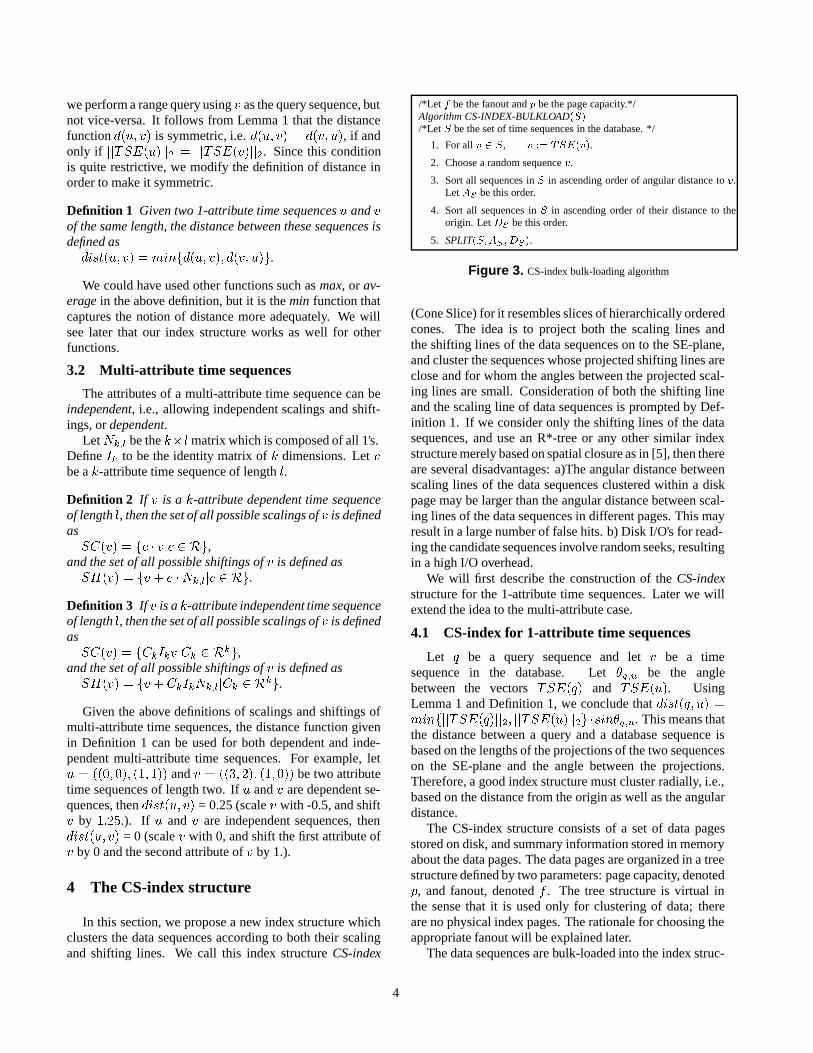
/*Let f be the fanout andp be the page capacity.*/Algorithm CS-INDEX-BULKLOAD(S)/*Let S be the set of time sequences in the database. */

1. For allv 2 S, v := TSE(v).

2. Choose a random sequencev.

3. Sort all sequences inS in ascending order of angular distance tov.LetAS be this order.

4. Sort all sequences inS in ascending order of their distance to theorigin. LetDS be this order.

5. SPLIT(S;AS ;DS).

Figure 3. CS-index bulk-loading algorithm

(Cone Slice) for it resembles slices of hierarchically orderedcones. The idea is to project both the scaling lines andthe shifting lines of the data sequences on to the SE-plane,and cluster the sequences whose projected shifting lines areclose and for whom the angles between the projected scal-ing lines are small. Consideration of both the shifting lineand the scaling line of data sequences is prompted by Def-inition 1. If we consider only the shifting lines of the datasequences, and use an R*-tree or any other similar indexstructure merely based on spatial closure as in [5], then thereare several disadvantages: a)The angular distance betweenscaling lines of the data sequences clustered within a diskpage may be larger than the angular distance between scal-ing lines of the data sequences in different pages. This mayresult in a large number of false hits. b) Disk I/O's for read-ing the candidate sequences involve random seeks, resultingin a high I/O overhead.

We will first describe the construction of theCS-indexstructure for the 1-attribute time sequences. Later we willextend the idea to the multi-attribute case.

4.1 CS-index for 1-attribute time sequences

Let q be a query sequence and letv be a timesequence in the database. Let�q;u be the anglebetween the vectorsTSE(q) and TSE(u). UsingLemma 1 and Definition 1, we conclude thatdist(q; u) =minfjjTSE(q)jj2; jjTSE(u)jj2g�sin�q;u. This means thatthe distance between a query and a database sequence isbased on the lengths of the projections of the two sequenceson the SE-plane and the angle between the projections.Therefore, a good index structure must cluster radially, i.e.,based on the distance from the origin as well as the angulardistance.

The CS-index structure consists of a set of data pagesstored on disk, and summary information stored in memoryabout the data pages. The data pages are organized in a treestructure defined by two parameters: page capacity, denotedp, and fanout, denotedf . The tree structure is virtual inthe sense that it is used only for clustering of data; thereare no physical index pages. The rationale for choosing theappropriate fanout will be explained later.

The data sequences are bulk-loaded into the index struc-

4

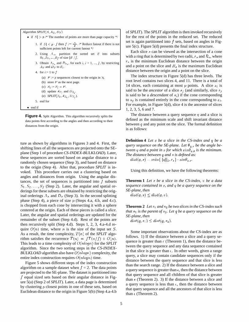
Algorithm SPLIT(S;AS; DS)

� if jSj > p /* The number of points are more than page capacity */

1. if jSj < p � f thenf :=jSj

p. /* Reduce fanout if there is not

sufficient points left for current fanout */

2. Using AS , partition the sorted setS into subsetsS1; S2; :::; Sf of sizejSj=f .

3. ObtainASiandDSi

, for eachi, i = 1, ...,f , by restrictingAS andDS to Si.

4. for i:= 1 tof

(a) P := p sequences closest to the origin inSi.

(b) storeP as the next page.

(c) Si := Si � P .

(d) updateASiandDSi

.

(e) SPLIT(Si; ASi; DSi

).

5. end for

� end if

Figure 4. Split Algorithm. This algorithm recursively splits the

data points first according to the angles and then according to their

distances from the origin.

ture as shown by algorithms in Figures 3 and 4. First, theshifting lines of all the sequences are projected onto the SE-plane (Step 1 of procedureCS-INDEX-BULKLOAD). Later,these sequences are sorted based on angular distance to arandomly chosen sequence (Step 3), and based on distanceto the origin (Step 4). After that, procedureSPLIT is in-voked. This procedure carries out a clustering based onangles and distances from origin. Using the angular dis-tances, the set of sequences is partitioned intof subsetsS1; S2; : : : ; Sf (Step 2). Later, the angular and spatial or-derings for these subsets are obtained by restricting the orig-inal orderingsAS andDS (Step 3). In the second splittingphase (Step 4), a piece of sizep (Steps 4.a, 4.b, and 4.c).is chopped from each cone by intersecting it with a spherecentered at the origin. Each of these pieces is called aslice.Later, the angular and spatial orderings are updated for theremainder of the subset (Step 4.d). Rest of the points arethen recursively split (Step 4.d). Steps 1, 2, 3, 4.a-4.d re-quireO(n) time, wheren is the size of the input setS.As a result, the time complexity,T (n) of theSPLIT algo-rithm satisfies the recurrenceT (n) = fT (n=f) + O(n).This leads to a time complexity ofO(nlogn) for theSPLITalgorithm. Since the two sorting steps in theCS-INDEX-BULKLOAD algorithm also haveO(nlogn) complexity, theentire index construction requiresO(nlogn) time.

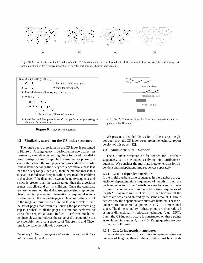
Figure 5 shows different steps of the index constructionalgorithm on a sample dataset whenf = 2. The data pointsare projected to the SE-plane. The dataset is partitioned intof equal sized sets based on their angular distance in Fig-ure 5(a) (Step 2 ofSPLIT). Later, a data page is determinedby clusteringp closest points in one of these sets, based onEuclidean distance to the origin in Figure 5(b) (Step 4.a-4.b

of SPLIT). TheSPLIT algorithm is then invoked recursivelyfor the rest of the points in the reduced set. The reducedset is again partitioned intof sets, based on angles in Fig-ure 5(c). Figure 5(d) presents the final index structure.

Each slices can be viewed as the intersection of a conewith a ring that is determined by two radii,rs andRs, wherers is the minimum Euclidean distance between the originand a point on the slice andRs is the maximum Euclideandistance between the origin and a point on the slice.

The index structure in Figure 5(d) has three levels. Theroot level contains two slices 4, and 11. There is a total of14 slices, each containing at mostp points. A slicesi issaid to be theancestor of a slicesj (and similarly, slicesjis said to be adescendant of si) if the cone correspondingto sj is contained entirely in the cone corresponding tosi.For example, in Figure 5(d), slice 4 is the ancestor of slices1, 2, 3, 5, 6 and 7.

The distance between a query sequenceq and a slice isdefined as the minimum scale and shift invariant distancebetweenq and any point on the slice. The formal definitionis as follows:

Definition 4 Let s be a slice in the CS-index and q be aquery sequence on the SE-plane. Let �q;s be the angle be-tween q and a point in s for which sin�q;s is the minimum.The distance between q and s is defined as:dist(q; s) = minfjjqjj2; rsg � sin�q;s.

Using this definition, we have the following theorems:

Theorem 1 Let s be a slice in the CS-index, v be a datasequence contained in s, and q be a query sequence on theSE-plane, thendist(q; s) � dist(q; v).

Theorem 2 Let s1 and s2 be two slices in the CS-index suchthat s1 is the parent of s2. Let q be a query sequence on theSE-plane, thendist(q; s1) � dist(q; s2).

Some important observations about the CS-index are asfollows. 1) If the distance between a slice and a query se-quence is greater than� (Theorem 1), then the distance be-tween the query sequence and any data sequence containedin that slice is greater than�. In other words, given a rangequery, a slice may contain candidate sequences only if thedistance between the query sequence and that slice is lessthan the search range. 2) If the distance between a slice anda query sequence is greater than�, then the distance betweenthat query sequence and all children of that slice is greaterthan� (Theorem 2). 3) If the distance between a slice anda query sequence is less than�, then the distance betweenthat query sequence and all the ancestors of that slice is lessthan� (Theorem 2).

5

��

��

��

��

��

��

��

��

��

��

��

��

��

��

��

��

��

��

��

��

��

��

��

��

��

��

��

��

��

��

��

��

��

��

��

��

��

��

��

��

��

��

��

��

��

��

��

��

��

��

��

��

��

��

��

��

��

��

��

��

��

��

��

��

��

��

��

��

��

��

��

��

��

��

��

S2S1��

��

��

��

��

��

��

��

��

��

��

��

��

��

��

��

��

��

��

��

��

��

��

��

��

��

��

��

��

��

��

��

��

��

��

��

��

��

��

��

��

��

��

��

��

��

��

��

��

��

��

��

��

��

��

��

��

��

��

��

��

��

��

��

��

��

��

��

��

��

��

��

��

��

��

��

��

��

��

��

��

��

��

��

��

��

��

��

��

��

��

��

��

��

��

��

��

��

��

��

��

��

��

��

��

��

��

��

��

��

��

��

��

��

��

��

��

��

��

��

��

��

��

��

��

��

��

��

��

��

��

��

��

��

��

��

��

��

��

��

��

��

��

��

��

��

��

��

��

��

��

��

��

��

��

��

��

��

��

��

��

��

��

��

��

��

��

��

��

��

��

��

��

��

��

��

��

��

��

��

��

��

��

��

��

��

��

��

��

��

��

��

��

��

��

��

��

��

��

��

��

��

(a)

��

��

��

��

��

��

��

��

��

��

��

��

��

��

��

��

��

��

��

��

��

��

��

��

��

��

��

��

��

��

��

��

��

��

��

��

��

��

��

��

��

��

��

��

��

��

��

��

��

��

��

��

��

��

S1- P1

P1

S2��

��

��

��

��

��

��

��

��

��

��

��

��

��

��

��

��

��

��

��

��

��

��

��

��

��

��

��

��

��

��

��

��

��

��

��

��

��

��

��

��

��

��

��

��

��

��

��

��

��

��

��

��

��

��

��

��

��

��

��

��

��

��

��

��

��

��

��

��

��

��

��

��

��

��

��

��

��

��

��

��

��

��

��

��

��

��

��

��

��

��

��

��

��

��

��

��

��

��

��

��

��

��

��

��

��

��

��

��

��

��

��

��

��

��

��

��

��

��

��

��

��

��

��

��

��

��

��

��

��

��

��

��

��

��

��

��

��

��

��

��

��

��

��

��

��

��

��

��

��

��

��

��

��

��

��

��

��

��

��

��

��

��

��

��

��

��

��

��

��

��

��

��

��

��

��

��

��

��

��

��

��

��

��

��

��

��

��

��

��

��

��

��

��

��

��

��

��

��

��

��

��

��

��

��

��

��

��

��

��

��

��

��

��

��

��

��

��

��

��

��

��

��

��

��

��

(b)

��

��

��

��

��

��

��

��

��

��

��

��

��

��

��

��

��

��

��

��

��

��

��

��

��

��

��

��

��

��

��

��

��

��

��

��

��

��

��

��

��

��

��

��

��

��

��

��

��

��

��

��

��

��

��

S11

S12

P1

S2��

��

��

��

��

��

��

��

��

��

��

��

��

��

��

��

��

��

��

��

��

��

��

��

��

��

��

��

��

��

��

��

��

��

��

��

��

��

��

��

��

��

��

��

��

��

��

��

��

��

��

��

��

��

��

��

��

��

��

��

��

��

��

��

��

��

��

��

��

��

��

��

��

��

��

��

��

��

��

��

��

��

��

��

��

��

��

��

��

��

��

��

��

��

��

��

��

��

��

��

��

��

��

��

��

��

��

��

��

��

��

��

��

��

��

��

��

��

��

��

��

��

��

��

��

��

��

��

��

��

��

��

��

��

��

��

��

��

��

��

��

��

��

��

��

��

��

��

��

��

��

��

��

��

��

��

��

��

��

��

��

��

��

��

��

��

��

��

��

��

��

��

��

��

��

��

��

��

��

��

��

��

��

��

��

��

��

��

��

��

��

��

��

��

��

��

��

��

��

��

��

��

��

��

��

��

��

��

��

��

��

��

��

��

��

��

��

��

��

��

��

��

��

��

��

(c)

1 2

3

4

5

6

7 8

9

11

12

13 14

10

(d)

Figure 5. Construction of the CS-index when f = 2. The data points are transformed onto shift eliminated plane. (a) Angular partitioning, (b)

spatial partitioning, (c) recursive invocation of angular partitioning, (d) final index structure.

Algorithm RANGE-QUERY(q, �)

1. C := ; /* the set of candidate pages*/

2. S := ; /* stack for navigation*/

3. Push all the root slices s1, s2, ..., sf on to S.

4. While S 6= ;

(a) s := Pop(S)

(b) if dist(q; s) � �

i. C := C [ fsg

ii. Push all the children of s on to S

5. Read the candidate pages in set C and perform postprocessing toeliminate false retrievals.

Figure 6. Range search algorithm

4.2 Similarity search on the CS-index structure

The range query algorithm on the CS-index is presentedin Figure 6. A range query is performed in two phases: anin-memory candidate generating phase followed by a disk-based post-processing step. In the in-memory phase, thesearch starts from the root pages and proceeds downwards.If the distance between the query sequence and a slice is lessthan the query range (Step 4.b), then the method marks thisslice as a candidate and expands the query to all the childrenof that slice. If the distance between the query sequence anda slice is greater than the search range, then the algorithmprunes that slice and all its children. Once the candidatesets are determined, the disk-based processing step begins.Using the disk placement information, a sequential scan isused to read all the candidate pages. Data points that are notin the range are pruned to ensure no false retrievals. Sincethe set of pages read from disk during the post-processingstep is a subset of all the pages, our method performs noworse than sequential scan. In fact, it performs much bet-ter since clustering reduces the range of the sequential scanconsiderably. As a consequence of Theorem 1 and Theo-rem 2, we have the following corollary:

Corollary 1 The range query algorithm in Figure 6 doesnot incur any false drops.

2Attr��

��

��

��

1Attr

Append Attributes

Reduce dimensionality

Project to SE-plane

Figure 7. Transformation of a 2-attribute dependent time se-

quence to the SE-plane.

We present a detailed discussion of the nearest neigh-bor queries on the CS-index structure in the technical reportversion of this paper [12].

4.3 Multi-attribute CS-index

The CS-index structure, so far defined for 1-attributesequences, can be extended easily to multi-attribute se-quences. We consider the multi-attribute extension for de-pendent and independent time sequences separately.

4.3.1 Case 1: dependent attributesIf the multi-attribute time sequences in the database are k-attribute dependent time sequences of length l, then theproblem reduces to the 1-attribute case by simply trans-forming the sequences into 1-attribute time sequences oflength k � l as in Figure 1. This is justified because all theentries are scaled and shifted by the same amount. Figure 7depicts how the dependent attributes are handled. These se-quences are considered as points in a (k � l)-dimensionalspace. The dimensionality of these points are then reducedusing a dimensionality reduction technique (e.g. DFT).Later, the CS-index structure is constructed on these pointsas explained in Figures 3, 4, and 5. Range queries are per-formed as in Figure 6.

4.3.2 Case 2: independent attributesIf the database consists of k-attribute independent time se-quences of length l, then all the attributes must be consid-

6

��

��

2Attr��

��

��

��

��

��

��

��

1Attr

Split Attributes

Reduce dimensionality

Project to SE-plane

Append Attributes

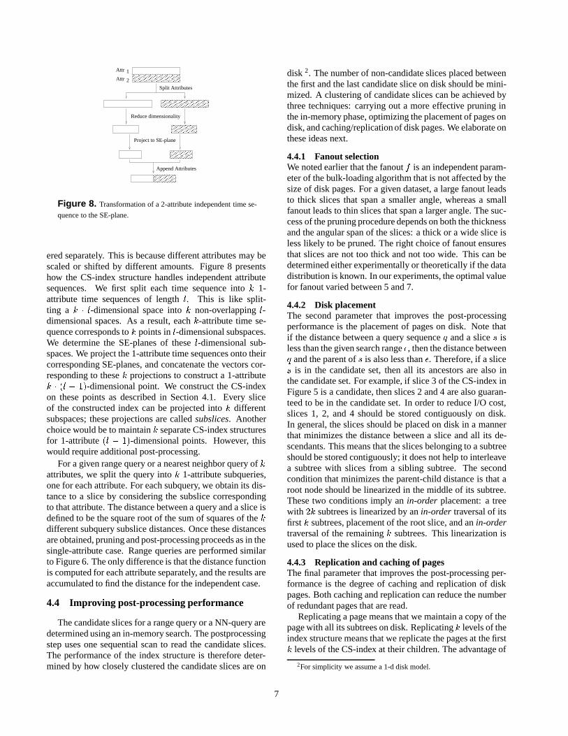
Figure 8. Transformation of a 2-attribute independent time se-

quence to the SE-plane.

ered separately. This is because different attributes may bescaled or shifted by different amounts. Figure 8 presentshow the CS-index structure handles independent attributesequences. We first split each time sequence into k 1-attribute time sequences of length l. This is like split-ting a k � l-dimensional space into k non-overlapping l-dimensional spaces. As a result, each k-attribute time se-quence corresponds to k points in l-dimensional subspaces.We determine the SE-planes of these l-dimensional sub-spaces. We project the 1-attribute time sequences onto theircorresponding SE-planes, and concatenate the vectors cor-responding to these k projections to construct a 1-attributek � (l � 1)-dimensional point. We construct the CS-indexon these points as described in Section 4.1. Every sliceof the constructed index can be projected into k differentsubspaces; these projections are called subslices. Anotherchoice would be to maintain k separate CS-index structuresfor 1-attribute (l � 1)-dimensional points. However, thiswould require additional post-processing.

For a given range query or a nearest neighbor query of kattributes, we split the query into k 1-attribute subqueries,one for each attribute. For each subquery, we obtain its dis-tance to a slice by considering the subslice correspondingto that attribute. The distance between a query and a slice isdefined to be the square root of the sum of squares of the kdifferent subquery subslice distances. Once these distancesare obtained, pruning and post-processing proceeds as in thesingle-attribute case. Range queries are performed similarto Figure 6. The only difference is that the distance functionis computed for each attribute separately, and the results areaccumulated to find the distance for the independent case.

4.4 Improving post-processing performance

The candidate slices for a range query or a NN-query aredetermined using an in-memory search. The postprocessingstep uses one sequential scan to read the candidate slices.The performance of the index structure is therefore deter-mined by how closely clustered the candidate slices are on

disk 2. The number of non-candidate slices placed betweenthe first and the last candidate slice on disk should be mini-mized. A clustering of candidate slices can be achieved bythree techniques: carrying out a more effective pruning inthe in-memory phase, optimizing the placement of pages ondisk, and caching/replication of disk pages. We elaborate onthese ideas next.

4.4.1 Fanout selectionWe noted earlier that the fanout f is an independent param-eter of the bulk-loading algorithm that is not affected by thesize of disk pages. For a given dataset, a large fanout leadsto thick slices that span a smaller angle, whereas a smallfanout leads to thin slices that span a larger angle. The suc-cess of the pruning procedure depends on both the thicknessand the angular span of the slices: a thick or a wide slice isless likely to be pruned. The right choice of fanout ensuresthat slices are not too thick and not too wide. This can bedetermined either experimentally or theoretically if the datadistribution is known. In our experiments, the optimal valuefor fanout varied between 5 and 7.

4.4.2 Disk placementThe second parameter that improves the post-processingperformance is the placement of pages on disk. Note thatif the distance between a query sequence q and a slice s isless than the given search range �, then the distance betweenq and the parent of s is also less than �. Therefore, if a slices is in the candidate set, then all its ancestors are also inthe candidate set. For example, if slice 3 of the CS-index inFigure 5 is a candidate, then slices 2 and 4 are also guaran-teed to be in the candidate set. In order to reduce I/O cost,slices 1, 2, and 4 should be stored contiguously on disk.In general, the slices should be placed on disk in a mannerthat minimizes the distance between a slice and all its de-scendants. This means that the slices belonging to a subtreeshould be stored contiguously; it does not help to interleavea subtree with slices from a sibling subtree. The secondcondition that minimizes the parent-child distance is that aroot node should be linearized in the middle of its subtree.These two conditions imply an in-order placement: a treewith 2k subtrees is linearized by an in-order traversal of itsfirst k subtrees, placement of the root slice, and an in-ordertraversal of the remaining k subtrees. This linearization isused to place the slices on the disk.

4.4.3 Replication and caching of pagesThe final parameter that improves the post-processing per-formance is the degree of caching and replication of diskpages. Both caching and replication can reduce the numberof redundant pages that are read.

Replicating a page means that we maintain a copy of thepage with all its subtrees on disk. Replicating k levels of theindex structure means that we replicate the pages at the firstk levels of the CS-index at their children. The advantage of

2For simplicity we assume a 1-d disk model.

7

Dataset Size R-tree Size CS-index Size

stock market dataset 2.5M 160K 25Kmotion dataset 8M 393K 41K

Table 1. The size of the R-tree and the CS-index structure for

stock market dataset and motion dataset.

replication is that it can reduce the distance between a pageand its ancestors. Replication works best if the queries aresufficiently narrow so that all candidate pages belong to asubtree and its ancestors. Otherwise, it can lead to redun-dant pages being read.

Caching k levels of the index structure means to keep thepages at the first k levels of the CS-index in memory and toplace the in-order linearizations of the subtrees at level kon disk. Unlike replication, caching can only improve theperformance of our index structure.

4.5 Extending the CS-index structure to othersymmetric distance functions

The CS-index structure can also be used when the dis-tance function is obtained by using max or avg functionsinstead of min function as follows:

Case 1. dist(q; u) = maxfd(q; u); d(u; q)g.In this case, one can prove that

dist(q; u) = maxfjjTSE(q)jj2; jjTSE(u)jj2g�sin�q;u.Similar to the min function, this distance function also usesa Euclidean distance and an angular distance in its compu-tation. The CS-index structure will work well for the maxfunction since it clusters time sequences based on the dis-tance from the origin as well as the angular distance.

Case 2. dist(q; u) = avgfd(q; u); d(u; q)g.dist(q; u) = (minfd(q;u);d(u;q)g+maxfd(q;u);d(u;q)g)

2.

Hence, dist(q; u) = jjTSE(q)jj2+jjTSE(u)jj22

� sin�q;u. Sim-ilar to min and max functions, avg function is also based onthe distance from the origin and the angular distance. As aresult of this, the CS-index structure will work well for theavg function too.

5 Experimental results

We carried out several experiments to test the perfor-mance of the CS-index structure. We used three differentdatasets in our experiments:

1) The first dataset is a stock market dataset, obtainedagain from chart.yahoo.com. The time sequences in thisdataset consist of 2 attributes. The first attribute is the clos-ing price, and the second attribute is the volume. There are20,000 time sequences of length 32 in this dataset.

2) The second dataset is obtained synthetically by con-sidering four different kinds of object trails in a 2-attributesequence. The motions that we consider are: bouncing ball,circular motion, billiard ball moving within the confines ofa rectangular table with perfect carom and elasticity, and a

0 0.001 0.002 0.003 0.004 0.005 0.006 0.007 0.008 0.009 0.010

50

100

150

200

250

300

Query Range

Dis

k I/O

Sequential ScanR−Tree CS−index Replicate−1 Replicate−2 Cache−1 Cache−2

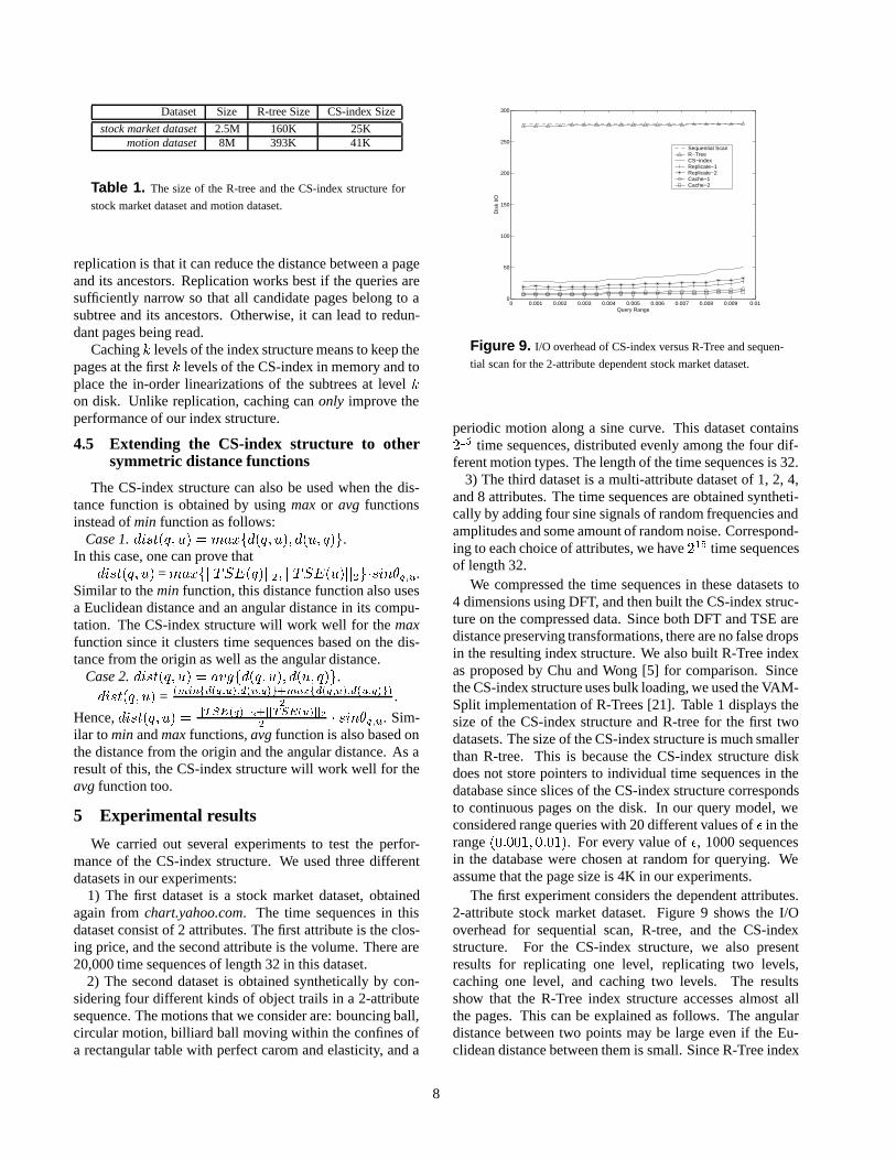
Figure 9. I/O overhead of CS-index versus R-Tree and sequen-

tial scan for the 2-attribute dependent stock market dataset.

periodic motion along a sine curve. This dataset contains215 time sequences, distributed evenly among the four dif-ferent motion types. The length of the time sequences is 32.

3) The third dataset is a multi-attribute dataset of 1, 2, 4,and 8 attributes. The time sequences are obtained syntheti-cally by adding four sine signals of random frequencies andamplitudes and some amount of random noise. Correspond-ing to each choice of attributes, we have 215 time sequencesof length 32.

We compressed the time sequences in these datasets to4 dimensions using DFT, and then built the CS-index struc-ture on the compressed data. Since both DFT and TSE aredistance preserving transformations, there are no false dropsin the resulting index structure. We also built R-Tree indexas proposed by Chu and Wong [5] for comparison. Sincethe CS-index structure uses bulk loading, we used the VAM-Split implementation of R-Trees [21]. Table 1 displays thesize of the CS-index structure and R-tree for the first twodatasets. The size of the CS-index structure is much smallerthan R-tree. This is because the CS-index structure diskdoes not store pointers to individual time sequences in thedatabase since slices of the CS-index structure correspondsto continuous pages on the disk. In our query model, weconsidered range queries with 20 different values of � in therange (0:001; 0:01). For every value of �, 1000 sequencesin the database were chosen at random for querying. Weassume that the page size is 4K in our experiments.

The first experiment considers the dependent attributes.2-attribute stock market dataset. Figure 9 shows the I/Ooverhead for sequential scan, R-tree, and the CS-indexstructure. For the CS-index structure, we also presentresults for replicating one level, replicating two levels,caching one level, and caching two levels. The resultsshow that the R-Tree index structure accesses almost allthe pages. This can be explained as follows. The angulardistance between two points may be large even if the Eu-clidean distance between them is small. Since R-Tree index

8

0 0.001 0.002 0.003 0.004 0.005 0.006 0.007 0.008 0.009 0.010

100

200

300

400

500

600

700

Query Range

Dis

k I/O

Sequential ScanCS−index Replicate−1 Replicate−2 Cache−1 Cache−2

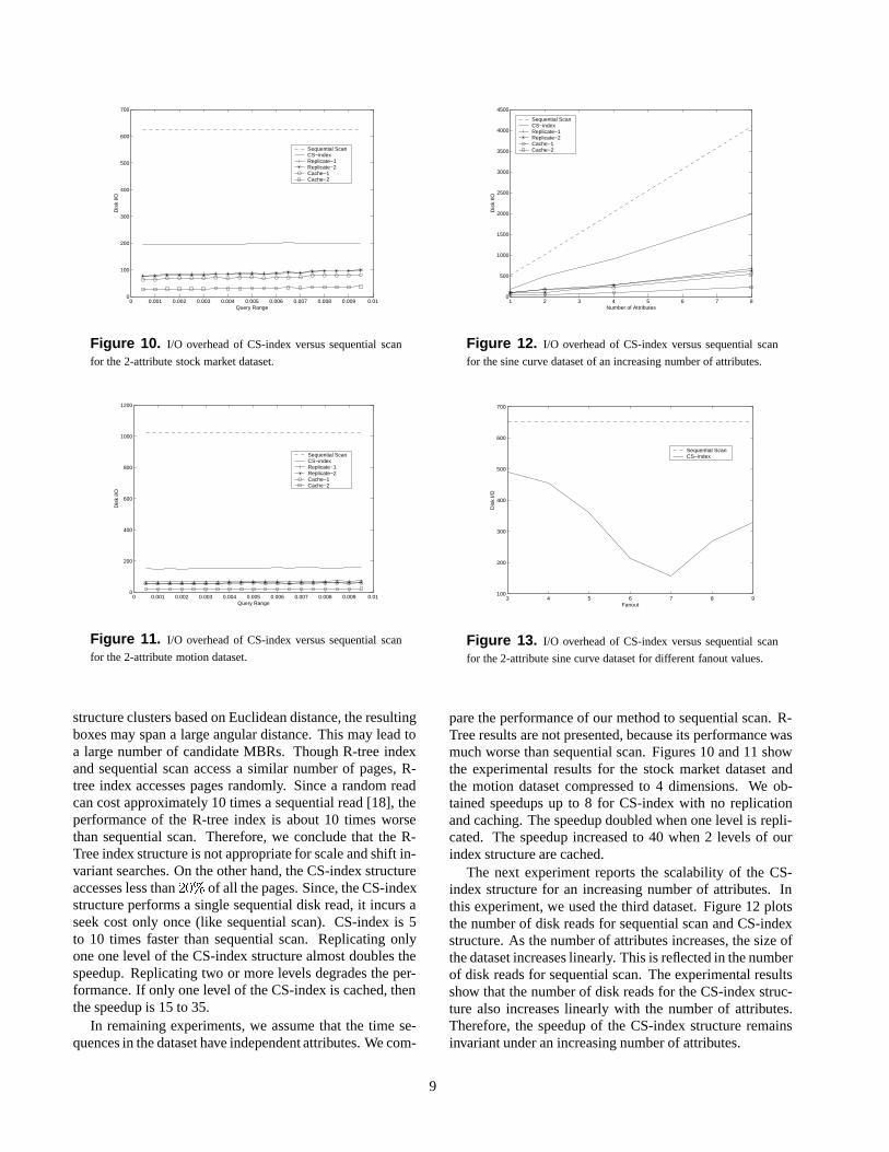
Figure 10. I/O overhead of CS-index versus sequential scan

for the 2-attribute stock market dataset.

0 0.001 0.002 0.003 0.004 0.005 0.006 0.007 0.008 0.009 0.010

200

400

600

800

1000

1200

Query Range

Dis

k I/O



for the 2-attribute motion dataset.

structure clusters based on Euclidean distance, the resultingboxes may span a large angular distance. This may lead toa large number of candidate MBRs. Though R-tree indexand sequential scan access a similar number of pages, R-tree index accesses pages randomly. Since a random readcan cost approximately 10 times a sequential read [18], theperformance of the R-tree index is about 10 times worsethan sequential scan. Therefore, we conclude that the R-Tree index structure is not appropriate for scale and shift in-variant searches. On the other hand, the CS-index structureaccesses less than 20% of all the pages. Since, the CS-indexstructure performs a single sequential disk read, it incurs aseek cost only once (like sequential scan). CS-index is 5to 10 times faster than sequential scan. Replicating onlyone one level of the CS-index structure almost doubles thespeedup. Replicating two or more levels degrades the per-formance. If only one level of the CS-index is cached, thenthe speedup is 15 to 35.

In remaining experiments, we assume that the time se-quences in the dataset have independent attributes. We com-

1 2 3 4 5 6 7 80

500

1000

1500

2000

2500

3000

3500

4000

4500

Number of Attributes

Dis

k I/O



for the sine curve dataset of an increasing number of attributes.

3 4 5 6 7 8 9100

200

300

400

500

600

700

Fanout

Dis

k I/O

Sequential ScanCS−index


for the 2-attribute sine curve dataset for different fanout values.

pare the performance of our method to sequential scan. R-Tree results are not presented, because its performance wasmuch worse than sequential scan. Figures 10 and 11 showthe experimental results for the stock market dataset andthe motion dataset compressed to 4 dimensions. We ob-tained speedups up to 8 for CS-index with no replicationand caching. The speedup doubled when one level is repli-cated. The speedup increased to 40 when 2 levels of ourindex structure are cached.

The next experiment reports the scalability of the CS-index structure for an increasing number of attributes. Inthis experiment, we used the third dataset. Figure 12 plotsthe number of disk reads for sequential scan and CS-indexstructure. As the number of attributes increases, the size ofthe dataset increases linearly. This is reflected in the numberof disk reads for sequential scan. The experimental resultsshow that the number of disk reads for the CS-index struc-ture also increases linearly with the number of attributes.Therefore, the speedup of the CS-index structure remainsinvariant under an increasing number of attributes.

9

Figure 13 plots the number of disk read for the CS-indexstructure for different values of fanout for the stock marketdata set compressed to 4 dimensions. The CS-index per-forms the best when the fanout is 7 for this data set. We ob-tained a similar U-shaped graph for the other datasets too.The optimal fanout for other datasets varies between 5 and7. Reason for this is explained in Section 4.4.1.

More comprehensive experimental results for additionaldatasets and a discussion for subsequence searches areavailable in the technical report version of this paper [12].

6 Discussion

We considered the problem of similarity search formulti-attribute sequences. First, we considered the simpleEuclidean distance metric. Later, we considered more chal-lenging metrics of shift and scale invariance. We formulateda new notion of similarity that is symmetric in allowingtransformations on both query and data sequences. Further-more, we do not impose any restriction on the shifting andscaling constants. We considered both the cases of whenthe scalings and the shiftings of the attributes are dependentand when they are independent.

We proposed a new index structure called CS-indexthat clusters time sequences according to their scalings andshiftings. This index structure recursively splits the searchspace into hierarchical cones and selects a slice of eachcone as a disk page. This index structure allows early prun-ing in the search phase. Later, we considered techniquesto improve the performance of the index structure: in-order based placement on disk, choice of right fanout, andcaching/replication. Finally, we showed that the method canbe extended to multi-attribute time sequences.

According to experimental results with both real andsynthetic datasets, our method performs 5 to 10 times fasterthan sequential scan. We also evaluated the effects ofreplicating higher levels of the index structure. Replicat-ing only the root level of the CS-index almost doubled theperformance of our method. Further replication eventu-ally degraded the performance. We also experimented withcaching. According to our experiments, if only the pagesat the root level are cached, our method performs 10 to 25times faster than sequential scan. We obtained speedup upto 45 when we cached one more level.

The techniques presented in this paper can be easilyextended to perform shift and scale invariant subsequencesearches. According to our experiments, our technique is 3times faster than sequential scan for subsequence searches.

Multi-attribute time sequences are an important emerg-ing class of applications. They arise ubiquitously and nat-urally: in medical applications, in control applications, invideo and event sequences, and in history-based applica-tions such as the stock market. The ability to query suchdata under different distance metrics is necessary for under-standing and analyzing the characteristics of such datasets.

The index structures presented in this paper are an impor-tant first step toward this, and should be widely applicable.

References

[1] R. Agrawal, C. Faloutsos, and A. Swami. Efficient similarity searchin sequence databases. In FODO, Evanston, Illinois, October 1993.

[2] R. Agrawal, K. Lin, H.S. Sawhney, and K. Shim. Fast similaritysearch in the presence of noise, scaling, and translation in time-seriesdatabases. In VLDB, Zurich, Switzerland, September 1995.

[3] N. Beckmann, H.-P. Kriegel, R. Schneider, and B. Seeger. The R*-tree: An efficient and robust access method for points and rectangles.In SIGMOD, pages 322–331, Atlantic City, NJ, 1990.

[4] K.-P. Chan and A.W.-C. Fu. Efficient time series matching bywavelets. In ICDE, 1999.

[5] K.K.W. Chu and M.H. Wong. Fast time-series searching with scalingand shifting. In PODS, Philadelphia, PA, 1999.

[6] G. Das, D. Gunopulos, and H. Mannila. Finding similar time series.In PKDD, pages 88–100, 1997.

[7] C. Faloutsos, M. Ranganathan, and Y. Manolopoulos. Fast subse-quence matching in time-series databases. In SIGMOD, pages 419–429, Minneapolis MN, May 1994.

[8] D. Q. Goldin and P. C. Kanellakis. On similarity queries for time-series data: Constraint specification and implementation. In CP,pages 137–153, France, September 1995.

[9] A. Guttman. R-trees: A dynamic index structure for spatial search-ing. In SIGMOD, pages 47–57, 1984.

[10] T. Kahveci and A. Singh. An efficient index structure for stringdatabases. In VLDB, pages 351–360, Roma, Italy, September 2001.

[11] T. Kahveci and A. Singh. Variable length queries for time series data.In ICDE, Heidelberg, Germany, 2001.

[12] T. Kahveci, A.K. Singh, and A. Gurel. Shift and scale invariantsearch of multi-attribute time sequences. Technical report, UCSB,2001.

[13] S.-L. Lee, S.-J. Chun, D.-H. Kim, J.-H. Lee, and C.-W. Chung. Sim-ilarity search for multidimensional data sequences. In ICDE, SanDiego, CA, 2000.

[14] C.-S. Perng, H. Wang, S.R. Zhang, and D.S. Parker. Landmarks:a new model for similarity-based pattern querying in time seriesdatabases. In ICDE, San Diego, USA, 2000.

[15] D. Rafiei. On similarity-based queries for time series data. In ICDE,Sydney, Australia, March 1999.

[16] D. Rafiei and A.O. Mendelzon. Similarity-based queries for timeseries data. In SIGMOD, pages 13–25, Tucson, AZ, 1997.

[17] D. Rafiei and A.O. Mendelzon. Efficient retrieval of similar timesequences using DFT. In FODO, Kobe, Japan, 1998.

[18] B. Seeger, P.-A. Larson, and R. McFayden. Reading a set of diskpages. In VLDB, pages 592–603, 1993.

[19] C. Shahabi, X. Tian, and W. Zhao. TSA-tree: A wavelet-basedapproach to improve the efficieny of multi-level surprise and trendqueries. In SSDBM, 2000.

[20] M. Vlachos, G. Kollios, and D. Gunopulos. Discovering similar mul-tidimensional trajectories. In ICDE, San Jose, CA, 2002.

[21] D. White and R. Jain. Similarity indexing: Algorithms and per-formance. In SPIE Storage and Retrieval for Image and VideoDatabases, 1996.

10

Similarity Searching for Multi-attribute Sequences · PDF fileSimilarity Searching for...

Documents

Transcript of Similarity Searching for Multi-attribute Sequences · PDF fileSimilarity Searching for...