Similarity of Semantic Relations - Cogprints
39
Similarity of Semantic Relations Peter D. Turney National Research Council Canada There are at least two kinds of similarity. Relational similarity is correspondence between re- lations, in contrast with attributional similarity, which is correspondence between attributes. When two words have a high degree of attributional similarity, we call them synonyms. When two pairs of words have a high degree of relational similarity, we say that their relations are anal- ogous. For example, the word pair mason:stone is analogous to the pair carpenter:wood. This paper introduces Latent Relational Analysis (LRA), a method for measuring relational similar- ity. LRA has potential applications in many areas, including information extraction, word sense disambiguation, and information retrieval. Recently the Vector Space Model (VSM) of informa- tion retrieval has been adapted to measuring relational similarity, achieving a score of 47% on a collection of 374 college-level multiple-choice word analogy questions. In the VSM approach, the relation between a pair of words is characterized by a vector of frequencies of predefined patterns in a large corpus. LRA extends the VSM approach in three ways: (1) the patterns are derived automatically from the corpus, (2) the Singular Value Decomposition (SVD) is used to smooth the frequency data, and (3) automatically generated synonyms are used to explore variations of the word pairs. LRA achieves 56% on the 374 analogy questions, statistically equivalent to the average human score of 57%. On the related problem of classifying semantic relations, LRA achieves similar gains over the VSM. 1. Introduction There are at least two kinds of similarity. Attributional similarity is correspondence be- tween attributes and relational similarity is correspondence between relations (Medin, Goldstone, and Gentner, 1990). When two words have a high degree of attributional similarity, we call them synonyms. When two word pairs have a high degree of rela- tional similarity, we say they are analogous. Verbal analogies are often written in the form A:B::C:D, meaning A is to B as C is to D; for example, traffic:street::water:riverbed. Traffic flows over a street; water flows over a riverbed. A street carries traffic; a riverbed carries water. There is a high degree of rela- tional similarity between the word pair traffic:street and the word pair water:riverbed. In fact, this analogy is the basis of several mathematical theories of traffic flow (Da- ganzo, 1994). In Section 2, we look more closely at the connections between attributional and re- lational similarity. In analogies such as mason:stone::carpenter:wood, it seems that re- lational similarity can be reduced to attributional similarity, since mason and carpenter are attributionally similar, as are stone and wood. In general, this reduction fails. Con- sider the analogy traffic:street::water:riverbed. Traffic and water are not attributionally similar. Street and riverbed are only moderately attributionally similar. Institute for Information Technology, National Research Council Canada, M-50 Montreal Road, Ottawa, Ontario, Canada, K1A 0R6. E-mail: [email protected]. Submission received: 30th March 2005; revised submission received: 10th November 2005; accepted for publication: 27th February 2006.
Transcript of Similarity of Semantic Relations - Cogprints
Similarity of Semantic Relations
Peter D. Turney�
National Research Council Canada
There are at least two kinds of similarity. Relational similarity is correspondence between re-
lations, in contrast with attributional similarity, which is correspondence between attributes.
When two words have a high degree of attributional similarity, we call them synonyms. When
two pairs of words have a high degree of relational similarity, we say that their relations are anal-
ogous. For example, the word pair mason:stone is analogous to the pair carpenter:wood. This
paper introduces Latent Relational Analysis (LRA), a method for measuring relational similar-
ity. LRA has potential applications in many areas, including information extraction, word sense
disambiguation, and information retrieval. Recently the Vector Space Model (VSM) of informa-
tion retrieval has been adapted to measuring relational similarity, achieving a score of 47% on a
collection of 374 college-level multiple-choice word analogy questions. In the VSM approach, the
relation between a pair of words is characterized by a vector of frequencies of predefined patterns
in a large corpus. LRA extends the VSM approach in three ways: (1) the patterns are derived
automatically from the corpus, (2) the Singular Value Decomposition (SVD) is used to smooth
the frequency data, and (3) automatically generated synonyms are used to explore variations of
the word pairs. LRA achieves 56% on the 374 analogy questions, statistically equivalent to the
average human score of 57%. On the related problem of classifying semantic relations, LRA
achieves similar gains over the VSM.
1. Introduction
There are at least two kinds of similarity. Attributional similarity is correspondence be-tween attributes and relational similarity is correspondence between relations (Medin,Goldstone, and Gentner, 1990). When two words have a high degree of attributionalsimilarity, we call them synonyms. When two word pairs have a high degree of rela-tional similarity, we say they are analogous.
Verbal analogies are often written in the form A:B::C:D, meaning A is to B as C is to D;for example, traffic:street::water:riverbed. Traffic flows over a street; water flows over ariverbed. A street carries traffic; a riverbed carries water. There is a high degree of rela-tional similarity between the word pair traffic:street and the word pair water:riverbed.In fact, this analogy is the basis of several mathematical theories of traffic flow (Da-ganzo, 1994).
In Section 2, we look more closely at the connections between attributional and re-lational similarity. In analogies such as mason:stone::carpenter:wood, it seems that re-lational similarity can be reduced to attributional similarity, since mason and carpenterare attributionally similar, as are stone and wood. In general, this reduction fails. Con-sider the analogy traffic:street::water:riverbed. Traffic and water are not attributionallysimilar. Street and riverbed are only moderately attributionally similar.
� Institute for Information Technology, National Research Council Canada, M-50 Montreal Road, Ottawa,Ontario, Canada, K1A 0R6. E-mail: [email protected].
Submission received: 30th March 2005; revised submission received: 10th November 2005; accepted forpublication: 27th February 2006.
Computational Linguistics Volume 1, Number 1
Many algorithms have been proposed for measuring the attributional similarity be-tween two words (Lesk, 1969; Resnik, 1995; Landauer and Dumais, 1997; Jiang andConrath, 1997; Lin, 1998b; Turney, 2001; Budanitsky and Hirst, 2001; Banerjee and Ped-ersen, 2003). Measures of attributional similarity have been studied extensively, due totheir applications in problems such as recognizing synonyms (Landauer and Dumais,1997), information retrieval (Deerwester et al., 1990), determining semantic orientation(Turney, 2002), grading student essays (Rehder et al., 1998), measuring textual cohesion(Morris and Hirst, 1991), and word sense disambiguation (Lesk, 1986).
On the other hand, since measures of relational similarity are not as well developedas measures of attributional similarity, the potential applications of relational similarityare not as well known. Many problems that involve semantic relations would benefitfrom an algorithm for measuring relational similarity. We discuss related problems innatural language processing, information retrieval, and information extraction in moredetail in Section 3.
This paper builds on the Vector Space Model (VSM) of information retrieval. Givena query, a search engine produces a ranked list of documents. The documents areranked in order of decreasing attributional similarity between the query and each doc-ument. Almost all modern search engines measure attributional similarity using theVSM (Baeza-Yates and Ribeiro-Neto, 1999). Turney and Littman (2005) adapt the VSMapproach to measuring relational similarity. They used a vector of frequencies of pat-terns in a corpus to represent the relation between a pair of words. Section 4 presentsthe VSM approach to measuring similarity.
In Section 5, we present an algorithm for measuring relational similarity, whichwe call Latent Relational Analysis (LRA). The algorithm learns from a large corpus ofunlabeled, unstructured text, without supervision. LRA extends the VSM approachof Turney and Littman (2005) in three ways: (1) The connecting patterns are derivedautomatically from the corpus, instead of using a fixed set of patterns. (2) SingularValue Decomposition (SVD) is used to smooth the frequency data. (3) Given a wordpair such as traffic:street, LRA considers transformations of the word pair, generated byreplacing one of the words by synonyms, such as traffic:road, traffic:highway.
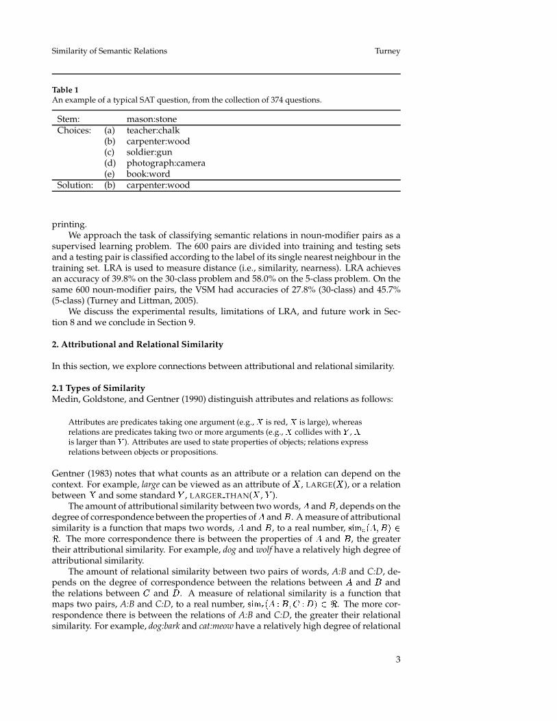
Section 6 presents our experimental evaluation of LRA with a collection of 374multiple-choice word analogy questions from the SAT college entrance exam.1 An ex-ample of a typical SAT question appears in Table 1. In the educational testing literature,the first pair (mason:stone) is called the stem of the analogy. The correct choice is calledthe solution and the incorrect choices are distractors. We evaluate LRA by testing its abil-ity to select the solution and avoid the distractors. The average performance of college-bound senior high school students on verbal SAT questions corresponds to an accuracyof about 57%. LRA achieves an accuracy of about 56%. On these same questions, theVSM attained 47%.
One application for relational similarity is classifying semantic relations in noun-modifier pairs (Turney and Littman, 2005). In Section 7, we evaluate the performanceof LRA with a set of 600 noun-modifier pairs from Nastase and Szpakowicz (2003). Theproblem is to classify a noun-modifier pair, such as “laser printer”, according to thesemantic relation between the head noun (printer) and the modifier (laser). The 600pairs have been manually labeled with 30 classes of semantic relations. For example,“laser printer” is classified as instrument; the printer uses the laser as an instrument for
�
The College Board eliminated analogies from the SAT in 2005, apparently because it was believed thatanalogy questions discriminate against minorities, although it has been argued by liberals (Goldenberg, 2005)that dropping analogy questions has increased discrimination against minorities and by conservatives (Kurtz,2002) that it has decreased academic standards. Analogy questions remain an important component in manyother tests, such as the GRE.
2
Similarity of Semantic Relations Turney
Table 1An example of a typical SAT question, from the collection of 374 questions.
Stem: mason:stoneChoices: (a) teacher:chalk
(b) carpenter:wood(c) soldier:gun(d) photograph:camera(e) book:word
Solution: (b) carpenter:wood
printing.We approach the task of classifying semantic relations in noun-modifier pairs as a
supervised learning problem. The 600 pairs are divided into training and testing setsand a testing pair is classified according to the label of its single nearest neighbour in thetraining set. LRA is used to measure distance (i.e., similarity, nearness). LRA achievesan accuracy of 39.8% on the 30-class problem and 58.0% on the 5-class problem. On thesame 600 noun-modifier pairs, the VSM had accuracies of 27.8% (30-class) and 45.7%(5-class) (Turney and Littman, 2005).
We discuss the experimental results, limitations of LRA, and future work in Sec-tion 8 and we conclude in Section 9.
2. Attributional and Relational Similarity
In this section, we explore connections between attributional and relational similarity.
2.1 Types of SimilarityMedin, Goldstone, and Gentner (1990) distinguish attributes and relations as follows:
Attributes are predicates taking one argument (e.g.,�
is red,�
is large), whereasrelations are predicates taking two or more arguments (e.g.,
�collides with � ,
�is larger than � ). Attributes are used to state properties of objects; relations expressrelations between objects or propositions.
Gentner (1983) notes that what counts as an attribute or a relation can depend on thecontext. For example, large can be viewed as an attribute of � , LARGE(� ), or a relationbetween � and some standard � , LARGER THAN(� , � ).
The amount of attributional similarity between two words, � and � , depends on thedegree of correspondence between the properties of � and � . A measure of attributionalsimilarity is a function that maps two words, � and � , to a real number, ��� � � � � �
. The more correspondence there is between the properties of � and � , the greatertheir attributional similarity. For example, dog and wolf have a relatively high degree ofattributional similarity.
The amount of relational similarity between two pairs of words, A:B and C:D, de-pends on the degree of correspondence between the relations between � and � andthe relations between � and � . A measure of relational similarity is a function thatmaps two pairs, A:B and C:D, to a real number, ��� � � � � � � � � � �
. The more cor-respondence there is between the relations of A:B and C:D, the greater their relationalsimilarity. For example, dog:bark and cat:meow have a relatively high degree of relational
3

Computational Linguistics Volume 1, Number 1
similarity.Cognitive scientists distinguish words that are semantically associated (bee–honey)
from words that are semantically similar (deer–pony), although they recognize that somewords are both associated and similar (doctor–nurse) (Chiarello et al., 1990). Both ofthese are types of attributional similarity, since they are based on correspondence be-tween attributes (e.g., bees and honey are both found in hives; deer and ponies are bothmammals).
Budanitsky and Hirst (2001) describe semantic relatedness as follows:
Recent research on the topic in computational linguistics has emphasized theperspective of semantic relatedness of two lexemes in a lexical resource, or itsinverse, semantic distance. It’s important to note that semantic relatedness is a moregeneral concept than similarity; similar entities are usually assumed to be relatedby virtue of their likeness (bank-trust company), but dissimilar entities may also besemantically related by lexical relationships such as meronymy (car-wheel) andantonymy (hot-cold), or just by any kind of functional relationship or frequentassociation (pencil-paper, penguin-Antarctica).
As these examples show, semantic relatedness is the same as attributional similarity(e.g., hot and cold are both kinds of temperature, pencil and paper are both used forwriting). Here we prefer to use the term attributional similarity, because it emphasizesthe contrast with relational similarity. The term semantic relatedness may lead to confu-sion when the term relational similarity is also under discussion.
Resnik (1995) describes semantic similarity as follows:
Semantic similarity represents a special case of semantic relatedness: for example,cars and gasoline would seem to be more closely related than, say, cars andbicycles, but the latter pair are certainly more similar. Rada et al. (1989) suggestthat the assessment of similarity in semantic networks can in fact be thought of asinvolving just taxonimic (IS-A) links, to the exclusion of other link types; that viewwill also be taken here, although admittedly it excludes some potentially usefulinformation.
Thus semantic similarity is a specific type of attributional similarity. The term semanticsimilarity is misleading, because it refers to a type of attributional similarity, yet rela-tional similarity is not any less semantic than attributional similarity.
To avoid confusion, we will use the terms attributional similarity and relational sim-ilarity, following Medin, Goldstone, and Gentner (1990). Instead of semantic similarity(Resnik, 1995) or semantically similar (Chiarello et al., 1990), we prefer the term taxonomi-cal similarity, which we take to be a specific type of attributional similarity. We interpretsynonymy as a high degree of attributional similarity. Analogy is a high degree of rela-tional similarity.
2.2 Measuring Attributional SimilarityAlgorithms for measuring attributional similarity can be lexicon-based (Lesk, 1986; Bu-danitsky and Hirst, 2001; Banerjee and Pedersen, 2003), corpus-based (Lesk, 1969; Lan-dauer and Dumais, 1997; Lin, 1998a; Turney, 2001), or a hybrid of the two (Resnik,1995; Jiang and Conrath, 1997; Turney et al., 2003). Intuitively, we might expect thatlexicon-based algorithms would be better at capturing synonymy than corpus-basedalgorithms, since lexicons, such as WordNet, explicitly provide synonymy informationthat is only implicit in a corpus. However, experiments do not support this intuition.
Several algorithms have been evaluated using 80 multiple-choice synonym ques-
4
Similarity of Semantic Relations Turney
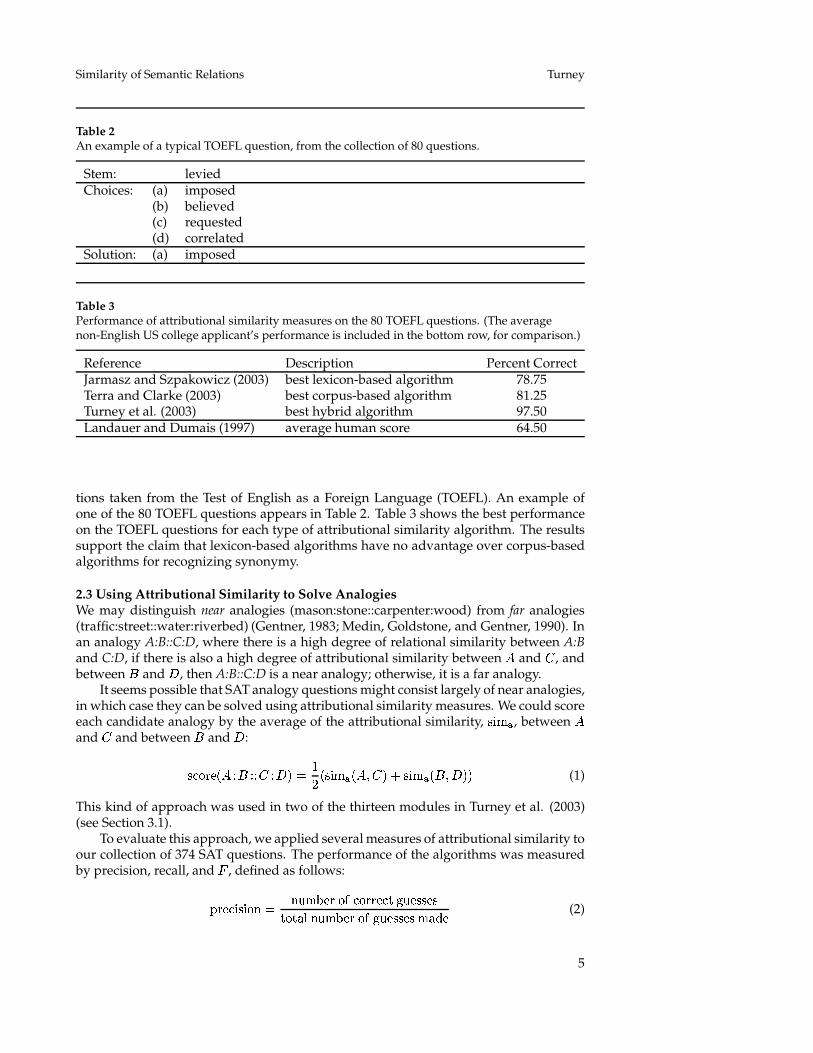
Table 2An example of a typical TOEFL question, from the collection of 80 questions.
Stem: leviedChoices: (a) imposed
(b) believed(c) requested(d) correlated
Solution: (a) imposed
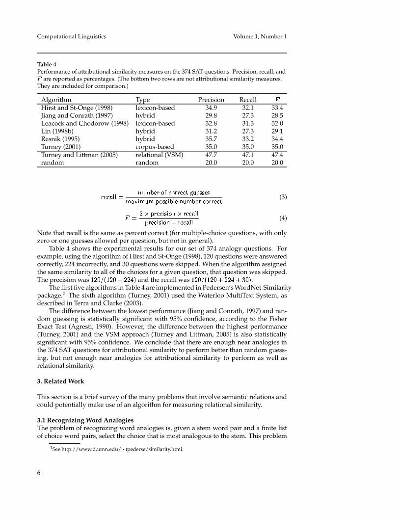
Table 3Performance of attributional similarity measures on the 80 TOEFL questions. (The averagenon-English US college applicant’s performance is included in the bottom row, for comparison.)
Reference Description Percent CorrectJarmasz and Szpakowicz (2003) best lexicon-based algorithm 78.75Terra and Clarke (2003) best corpus-based algorithm 81.25Turney et al. (2003) best hybrid algorithm 97.50Landauer and Dumais (1997) average human score 64.50
tions taken from the Test of English as a Foreign Language (TOEFL). An example ofone of the 80 TOEFL questions appears in Table 2. Table 3 shows the best performanceon the TOEFL questions for each type of attributional similarity algorithm. The resultssupport the claim that lexicon-based algorithms have no advantage over corpus-basedalgorithms for recognizing synonymy.
2.3 Using Attributional Similarity to Solve AnalogiesWe may distinguish near analogies (mason:stone::carpenter:wood) from far analogies(traffic:street::water:riverbed) (Gentner, 1983; Medin, Goldstone, and Gentner, 1990). Inan analogy A:B::C:D, where there is a high degree of relational similarity between A:Band C:D, if there is also a high degree of attributional similarity between � and � , andbetween � and � , then A:B::C:D is a near analogy; otherwise, it is a far analogy.
It seems possible that SAT analogy questions might consist largely of near analogies,in which case they can be solved using attributional similarity measures. We could scoreeach candidate analogy by the average of the attributional similarity, ��� , between �and � and between � and � :
����� � �� ��� �� � ��� ��� � � � � � ��� � � � �� (1)
This kind of approach was used in two of the thirteen modules in Turney et al. (2003)(see Section 3.1).
To evaluate this approach, we applied several measures of attributional similarity toour collection of 374 SAT questions. The performance of the algorithms was measuredby precision, recall, and � , defined as follows:
������� � ����� � ������� ������������ ����� � ������� � ��� (2)
5
Computational Linguistics Volume 1, Number 1
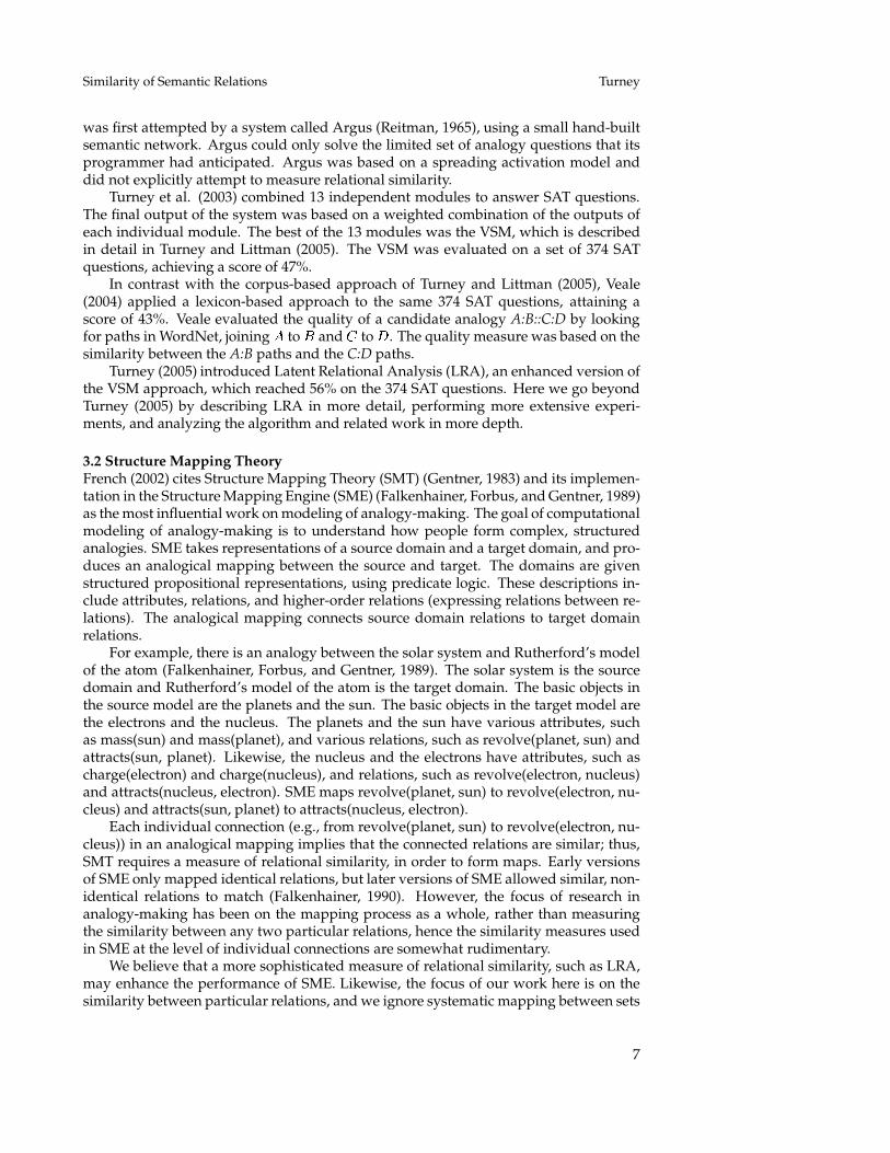
Table 4Performance of attributional similarity measures on the 374 SAT questions. Precision, recall, and�
are reported as percentages. (The bottom two rows are not attributional similarity measures.They are included for comparison.)
Algorithm Type Precision Recall �Hirst and St-Onge (1998) lexicon-based 34.9 32.1 33.4Jiang and Conrath (1997) hybrid 29.8 27.3 28.5Leacock and Chodorow (1998) lexicon-based 32.8 31.3 32.0Lin (1998b) hybrid 31.2 27.3 29.1Resnik (1995) hybrid 35.7 33.2 34.4Turney (2001) corpus-based 35.0 35.0 35.0Turney and Littman (2005) relational (VSM) 47.7 47.1 47.4random random 20.0 20.0 20.0
������ � ����� � ������� �������� �� ���� ������� ����� ������� (3)
� �� � ������� � ��������� ���� � ������ (4)
Note that recall is the same as percent correct (for multiple-choice questions, with onlyzero or one guesses allowed per question, but not in general).
Table 4 shows the experimental results for our set of 374 analogy questions. Forexample, using the algorithm of Hirst and St-Onge (1998), 120 questions were answeredcorrectly, 224 incorrectly, and 30 questions were skipped. When the algorithm assignedthe same similarity to all of the choices for a given question, that question was skipped.The precision was
���� ��� � ��� � and the recall was���� ��� � ��� � ���.
The first five algorithms in Table 4 are implemented in Pedersen’s WordNet-Similaritypackage.2 The sixth algorithm (Turney, 2001) used the Waterloo MultiText System, asdescribed in Terra and Clarke (2003).
The difference between the lowest performance (Jiang and Conrath, 1997) and ran-dom guessing is statistically significant with 95% confidence, according to the FisherExact Test (Agresti, 1990). However, the difference between the highest performance(Turney, 2001) and the VSM approach (Turney and Littman, 2005) is also statisticallysignificant with 95% confidence. We conclude that there are enough near analogies inthe 374 SAT questions for attributional similarity to perform better than random guess-ing, but not enough near analogies for attributional similarity to perform as well asrelational similarity.
3. Related Work
This section is a brief survey of the many problems that involve semantic relations andcould potentially make use of an algorithm for measuring relational similarity.
3.1 Recognizing Word AnalogiesThe problem of recognizing word analogies is, given a stem word pair and a finite listof choice word pairs, select the choice that is most analogous to the stem. This problem
�See http://www.d.umn.edu/�tpederse/similarity.html.
6
Similarity of Semantic Relations Turney
was first attempted by a system called Argus (Reitman, 1965), using a small hand-builtsemantic network. Argus could only solve the limited set of analogy questions that itsprogrammer had anticipated. Argus was based on a spreading activation model anddid not explicitly attempt to measure relational similarity.
Turney et al. (2003) combined 13 independent modules to answer SAT questions.The final output of the system was based on a weighted combination of the outputs ofeach individual module. The best of the 13 modules was the VSM, which is describedin detail in Turney and Littman (2005). The VSM was evaluated on a set of 374 SATquestions, achieving a score of 47%.
In contrast with the corpus-based approach of Turney and Littman (2005), Veale(2004) applied a lexicon-based approach to the same 374 SAT questions, attaining ascore of 43%. Veale evaluated the quality of a candidate analogy A:B::C:D by lookingfor paths in WordNet, joining � to � and � to � . The quality measure was based on thesimilarity between the A:B paths and the C:D paths.
Turney (2005) introduced Latent Relational Analysis (LRA), an enhanced version ofthe VSM approach, which reached 56% on the 374 SAT questions. Here we go beyondTurney (2005) by describing LRA in more detail, performing more extensive experi-ments, and analyzing the algorithm and related work in more depth.
3.2 Structure Mapping TheoryFrench (2002) cites Structure Mapping Theory (SMT) (Gentner, 1983) and its implemen-tation in the Structure Mapping Engine (SME) (Falkenhainer, Forbus, and Gentner, 1989)as the most influential work on modeling of analogy-making. The goal of computationalmodeling of analogy-making is to understand how people form complex, structuredanalogies. SME takes representations of a source domain and a target domain, and pro-duces an analogical mapping between the source and target. The domains are givenstructured propositional representations, using predicate logic. These descriptions in-clude attributes, relations, and higher-order relations (expressing relations between re-lations). The analogical mapping connects source domain relations to target domainrelations.
For example, there is an analogy between the solar system and Rutherford’s modelof the atom (Falkenhainer, Forbus, and Gentner, 1989). The solar system is the sourcedomain and Rutherford’s model of the atom is the target domain. The basic objects inthe source model are the planets and the sun. The basic objects in the target model arethe electrons and the nucleus. The planets and the sun have various attributes, suchas mass(sun) and mass(planet), and various relations, such as revolve(planet, sun) andattracts(sun, planet). Likewise, the nucleus and the electrons have attributes, such ascharge(electron) and charge(nucleus), and relations, such as revolve(electron, nucleus)and attracts(nucleus, electron). SME maps revolve(planet, sun) to revolve(electron, nu-cleus) and attracts(sun, planet) to attracts(nucleus, electron).
Each individual connection (e.g., from revolve(planet, sun) to revolve(electron, nu-cleus)) in an analogical mapping implies that the connected relations are similar; thus,SMT requires a measure of relational similarity, in order to form maps. Early versionsof SME only mapped identical relations, but later versions of SME allowed similar, non-identical relations to match (Falkenhainer, 1990). However, the focus of research inanalogy-making has been on the mapping process as a whole, rather than measuringthe similarity between any two particular relations, hence the similarity measures usedin SME at the level of individual connections are somewhat rudimentary.
We believe that a more sophisticated measure of relational similarity, such as LRA,may enhance the performance of SME. Likewise, the focus of our work here is on thesimilarity between particular relations, and we ignore systematic mapping between sets
7
Computational Linguistics Volume 1, Number 1
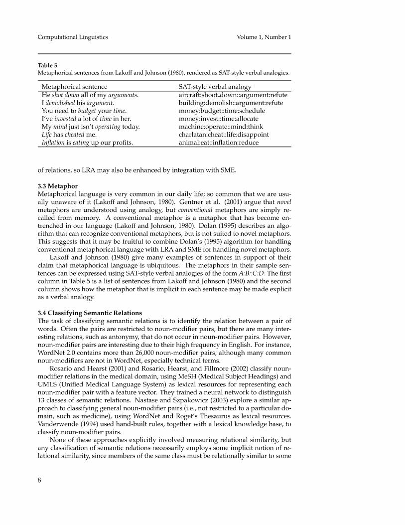
Table 5Metaphorical sentences from Lakoff and Johnson (1980), rendered as SAT-style verbal analogies.
Metaphorical sentence SAT-style verbal analogyHe shot down all of my arguments. aircraft:shoot down::argument:refuteI demolished his argument. building:demolish::argument:refuteYou need to budget your time. money:budget::time:scheduleI’ve invested a lot of time in her. money:invest::time:allocateMy mind just isn’t operating today. machine:operate::mind:thinkLife has cheated me. charlatan:cheat::life:disappointInflation is eating up our profits. animal:eat::inflation:reduce
of relations, so LRA may also be enhanced by integration with SME.
3.3 MetaphorMetaphorical language is very common in our daily life; so common that we are usu-ally unaware of it (Lakoff and Johnson, 1980). Gentner et al. (2001) argue that novelmetaphors are understood using analogy, but conventional metaphors are simply re-called from memory. A conventional metaphor is a metaphor that has become en-trenched in our language (Lakoff and Johnson, 1980). Dolan (1995) describes an algo-rithm that can recognize conventional metaphors, but is not suited to novel metaphors.This suggests that it may be fruitful to combine Dolan’s (1995) algorithm for handlingconventional metaphorical language with LRA and SME for handling novel metaphors.
Lakoff and Johnson (1980) give many examples of sentences in support of theirclaim that metaphorical language is ubiquitous. The metaphors in their sample sen-tences can be expressed using SAT-style verbal analogies of the form A:B::C:D. The firstcolumn in Table 5 is a list of sentences from Lakoff and Johnson (1980) and the secondcolumn shows how the metaphor that is implicit in each sentence may be made explicitas a verbal analogy.
3.4 Classifying Semantic RelationsThe task of classifying semantic relations is to identify the relation between a pair ofwords. Often the pairs are restricted to noun-modifier pairs, but there are many inter-esting relations, such as antonymy, that do not occur in noun-modifier pairs. However,noun-modifier pairs are interesting due to their high frequency in English. For instance,WordNet 2.0 contains more than 26,000 noun-modifier pairs, although many commonnoun-modifiers are not in WordNet, especially technical terms.
Rosario and Hearst (2001) and Rosario, Hearst, and Fillmore (2002) classify noun-modifier relations in the medical domain, using MeSH (Medical Subject Headings) andUMLS (Unified Medical Language System) as lexical resources for representing eachnoun-modifier pair with a feature vector. They trained a neural network to distinguish13 classes of semantic relations. Nastase and Szpakowicz (2003) explore a similar ap-proach to classifying general noun-modifier pairs (i.e., not restricted to a particular do-main, such as medicine), using WordNet and Roget’s Thesaurus as lexical resources.Vanderwende (1994) used hand-built rules, together with a lexical knowledge base, toclassify noun-modifier pairs.
None of these approaches explicitly involved measuring relational similarity, butany classification of semantic relations necessarily employs some implicit notion of re-lational similarity, since members of the same class must be relationally similar to some
8
Similarity of Semantic Relations Turney
extent. Barker and Szpakowicz (1998) tried a corpus-based approach that explicitlyused a measure of relational similarity, but their measure was based on literal matching,which limited its ability to generalize. Moldovan et al. (2004) also used a measure ofrelational similarity, based on mapping each noun and modifier into semantic classesin WordNet. The noun-modifier pairs were taken from a corpus and the surroundingcontext in the corpus was used in a word sense disambiguation algorithm, to improvethe mapping of the noun and modifier into WordNet. Turney and Littman (2005) usedthe VSM (as a component in a single nearest neighbour learning algorithm) to measurerelational similarity. We take the same approach here, substituting LRA for the VSM, inSection 7.
Lauer (1995) used a corpus-based approach (using the BNC) to paraphrase noun-modifier pairs, by inserting the prepositions of, for, in, at, on, from, with, and about. Forexample, reptile haven was paraphrased as haven for reptiles. Lapata and Keller (2004)achieved improved results on this task, by using the database of AltaVista’s search en-gine as a corpus.
3.5 Word Sense DisambiguationWe believe that the intended sense of a polysemous word is determined by its semanticrelations with the other words in the surrounding text. If we can identify the semanticrelations between the given word and its context, then we can disambiguate the givenword. Yarowsky’s (1993) observation that collocations are almost always monosemousis evidence for this view. Federici, Montemagni, and Pirrelli (1997) present an analogy-based approach to word sense disambiguation.
For example, consider the word plant. Out of context, plant could refer to an in-dustrial plant or a living organism. Suppose plant appears in some text near food. Atypical approach to disambiguating plant would compare the attributional similarity offood and industrial plant to the attributional similarity of food and living organism (Lesk,1986; Banerjee and Pedersen, 2003). In this case, the decision may not be clear, since in-dustrial plants often produce food and living organisms often serve as food. It would bevery helpful to know the relation between food and plant in this example. In the phrase“food for the plant”, the relation between food and plant strongly suggests that the plantis a living organism, since industrial plants do not need food. In the text “food at theplant”, the relation strongly suggests that the plant is an industrial plant, since livingorganisms are not usually considered as locations. Thus an algorithm for classifyingsemantic relations (as in Section 7) should be helpful for word sense disambiguation.
3.6 Information ExtractionThe problem of relation extraction is, given an input document and a specific relation � ,extract all pairs of entities (if any) that have the relation � in the document. The prob-lem was introduced as part of the Message Understanding Conferences (MUC) in 1998.Zelenko, Aone, and Richardella (2003) present a kernel method for extracting the rela-tions person-affiliation and organization-location. For example, in the sentence “John Smithis the chief scientist of the Hardcom Corporation,” there is a person-affiliation relationbetween “John Smith” and “Hardcom Corporation” (Zelenko, Aone, and Richardella,2003). This is similar to the problem of classifying semantic relations (Section 3.4), ex-cept that information extraction focuses on the relation between a specific pair of entitiesin a specific document, rather than a general pair of words in general text. Therefore analgorithm for classifying semantic relations should be useful for information extraction.
In the VSM approach to classifying semantic relations (Turney and Littman, 2005),we would have a training set of labeled examples of the relation person-affiliation, for in-stance. Each example would be represented by a vector of pattern frequencies. Given a
9
Computational Linguistics Volume 1, Number 1
specific document discussing “John Smith” and “Hardcom Corporation”, we could con-struct a vector representing the relation between these two entities, and then measurethe relational similarity between this unlabeled vector and each of our labeled trainingvectors. It would seem that there is a problem here, because the training vectors wouldbe relatively dense, since they would presumably be derived from a large corpus, butthe new unlabeled vector for “John Smith” and “Hardcom Corporation” would be verysparse, since these entities might be mentioned only once in the given document. How-ever, this is not a new problem for the Vector Space Model; it is the standard situationwhen the VSM is used for information retrieval. A query to a search engine is rep-resented by a very sparse vector whereas a document is represented by a relativelydense vector. There are well-known techniques in information retrieval for coping withthis disparity, such as weighting schemes for query vectors that are different from theweighting schemes for document vectors (Salton and Buckley, 1988).
3.7 Question AnsweringIn their paper on classifying semantic relations, Moldovan et al. (2004) suggest that animportant application of their work is Question Answering. As defined in the Text RE-trieval Conference (TREC) Question Answering (QA) track, the task is to answer simplequestions, such as “Where have nuclear incidents occurred?”, by retrieving a relevantdocument from a large corpus and then extracting a short string from the document,such as “The Three Mile Island nuclear incident caused a DOE policy crisis.” Moldovanet al. (2004) propose to map a given question to a semantic relation and then search forthat relation in a corpus of semantically tagged text. They argue that the desired se-mantic relation can easily be inferred from the surface form of the question. A questionof the form “Where ...?” is likely to be seeking for entities with a location relation anda question of the form “What did ... make?” is likely to be looking for entities with aproduct relation. In Section 7, we show how LRA can recognize relations such as locationand product (see Table 19).
3.8 Automatic Thesaurus GenerationHearst (1992) presents an algorithm for learning hyponym (type of) relations from a cor-pus and Berland and Charniak (1999) describe how to learn meronym (part of) relationsfrom a corpus. These algorithms could be used to automatically generate a thesaurus ordictionary, but we would like to handle more relations than hyponymy and meronymy.WordNet distinguishes more than a dozen semantic relations between words (Fellbaum,1998) and Nastase and Szpakowicz (2003) list 30 semantic relations for noun-modifierpairs. Hearst (1992) and Berland and Charniak (1999) use manually generated rules tomine text for semantic relations. Turney and Littman (2005) also use a manually gener-ated set of 64 patterns.
LRA does not use a predefined set of patterns; it learns patterns from a large corpus.Instead of manually generating new rules or patterns for each new semantic relation,it is possible to automatically learn a measure of relational similarity that can handlearbitrary semantic relations. A nearest neighbour algorithm can then use this relationalsimilarity measure to learn to classify according to any set of classes of relations, giventhe appropriate labeled training data.
Girju, Badulescu, and Moldovan (2003) present an algorithm for learning meronymrelations from a corpus. Like Hearst (1992) and Berland and Charniak (1999), they usemanually generated rules to mine text for their desired relation. However, they supple-ment their manual rules with automatically learned constraints, to increase the precisionof the rules.
10
Similarity of Semantic Relations Turney
3.9 Information RetrievalVeale (2003) has developed an algorithm for recognizing certain types of word analo-gies, based on information in WordNet. He proposes to use the algorithm for ana-logical information retrieval. For example, the query “Muslim church” should return“mosque” and the query “Hindu bible” should return “the Vedas”. The algorithm wasdesigned with a focus on analogies of the form adjective:noun::adjective:noun, such asChristian:church::Muslim:mosque.
A measure of relational similarity is applicable to this task. Given a pair of words,� and � , the task is to return another pair of words, � and � , such that there is highrelational similarity between the pair � :� and the pair � :� . For example, given � =“Muslim” and � = “church”, return � = “mosque” and � = “Christian”. (The pairMuslim:mosque has a high relational similarity to the pair Christian:church.)
Marx et al. (2002) developed an unsupervised algorithm for discovering analogiesby clustering words from two different corpora. Each cluster of words in one corpusis coupled one-to-one with a cluster in the other corpus. For example, one experimentused a corpus of Buddhist documents and a corpus of Christian documents. A cluster ofwords such as �Hindu, Mahayana, Zen, ...� from the Buddhist corpus was coupled witha cluster of words such as �Catholic, Protestant, ...� from the Christian corpus. Thus thealgorithm appears to have discovered an analogical mapping between Buddhist schoolsand traditions and Christian schools and traditions. This is interesting work, but it isnot directly applicable to SAT analogies, because it discovers analogies between clustersof words, rather than individual words.
3.10 Identifying Semantic RolesA semantic frame for an event such as judgement contains semantic roles such as judge,evaluee, and reason, whereas an event such as statement contains roles such as speaker,addressee, and message (Gildea and Jurafsky, 2002). The task of identifying semantic rolesis to label the parts of a sentence according to their semantic roles. We believe that itmay be helpful to view semantic frames and their semantic roles as sets of semanticrelations; thus a measure of relational similarity should help us to identify semanticroles. Moldovan et al. (2004) argue that semantic roles are merely a special case ofsemantic relations (Section 3.4), since semantic roles always involve verbs or predicates,but semantic relations can involve words of any part of speech.
4. The Vector Space Model
This section examines past work on measuring attributional and relational similarityusing the Vector Space Model (VSM).
4.1 Measuring Attributional Similarity with the Vector Space ModelThe VSM was first developed for information retrieval (Salton and McGill, 1983; Saltonand Buckley, 1988; Salton, 1989) and it is at the core of most modern search engines(Baeza-Yates and Ribeiro-Neto, 1999). In the VSM approach to information retrieval,queries and documents are represented by vectors. Elements in these vectors are basedon the frequencies of words in the corresponding queries and documents. The frequen-cies are usually transformed by various formulas and weights, tailored to improve theeffectiveness of the search engine (Salton, 1989). The attributional similarity between aquery and a document is measured by the cosine of the angle between their correspond-ing vectors. For a given query, the search engine sorts the matching documents in orderof decreasing cosine.
The VSM approach has also been used to measure the attributional similarity of
11

Computational Linguistics Volume 1, Number 1
words (Lesk, 1969; Ruge, 1992; Pantel and Lin, 2002). Pantel and Lin (2002) clusteredwords according to their attributional similarity, as measured by a VSM. Their algo-rithm is able to discover the different senses of polysemous words, using unsupervisedlearning.
Latent Semantic Analysis enhances the VSM approach to information retrieval byusing the Singular Value Decomposition (SVD) to smooth the vectors, which helps tohandle noise and sparseness in the data (Deerwester et al., 1990; Dumais, 1993; Lan-dauer and Dumais, 1997). SVD improves both document-query attributional similaritymeasures (Deerwester et al., 1990; Dumais, 1993) and word-word attributional similar-ity measures (Landauer and Dumais, 1997). LRA also uses SVD to smooth vectors, aswe discuss in Section 5.
4.2 Measuring Relational Similarity with the Vector Space ModelLet � � be the semantic relation (or set of relations) between a pair of words, � and � ,and let � � be the semantic relation (or set of relations) between another pair, � and� . We wish to measure the relational similarity between � � and � � . The relations � �and � � are not given to us; our task is to infer these hidden (latent) relations and thencompare them.
In the VSM approach to relational similarity (Turney and Littman, 2005), we createvectors, �� and �� , that represent features of � � and � � , and then measure the similarityof � � and � � by the cosine of the angle
�between �� and �� :
� � � ��� �� � � � � � � ��� � (5)
�� � ��� �� � � � � �� �� � (6)
�� ��� � � �
�� � � �� � �� � ��� � �� �� � �� � �� � ��� �� � ����� � �� � ��� � �� � � � � ����� � � ��� � (7)
We create a vector, � , to characterize the relationship between two words, � and� , by counting the frequencies of various short phrases containing � and � . Turneyand Littman (2005) use a list of 64 joining terms, such as “of”, “for”, and “to”, to form128 phrases that contain � and � , such as “� of � ”, “� of � ”, “� for � ”, “� for� ”, “� to � ”, and “� to � ”. These phrases are then used as queries for a searchengine and the number of hits (matching documents) is recorded for each query. Thisprocess yields a vector of 128 numbers. If the number of hits for a query is �, thenthe corresponding element in the vector � is ��� � � ��. Several authors report that thelogarithmic transformation of frequencies improves cosine-based similarity measures(Salton and Buckley, 1988; Ruge, 1992; Lin, 1998b).
Turney and Littman (2005) evaluated the VSM approach by its performance on 374SAT analogy questions, achieving a score of 47%. Since there are five choices for eachquestion, the expected score for random guessing is 20%. To answer a multiple-choiceanalogy question, vectors are created for the stem pair and each choice pair, and thencosines are calculated for the angles between the stem pair and each choice pair. Thebest guess is the choice pair with the highest cosine. We use the same set of analogyquestions to evaluate LRA in Section 6.
The VSM was also evaluated by its performance as a distance (nearness) measure ina supervised nearest neighbour classifier for noun-modifier semantic relations (Turney
12
Similarity of Semantic Relations Turney
and Littman, 2005). The evaluation used 600 hand-labeled noun-modifier pairs fromNastase and Szpakowicz (2003). A testing pair is classified by searching for its singlenearest neighbour in the labeled training data. The best guess is the label for the trainingpair with the highest cosine. LRA is evaluated with the same set of noun-modifier pairsin Section 7.
Turney and Littman (2005) used the AltaVista search engine to obtain the frequencyinformation required to build vectors for the VSM. Thus their corpus was the set of allweb pages indexed by AltaVista. At the time, the English subset of this corpus consistedof about � � �� �� words. Around April 2004, AltaVista made substantial changes totheir search engine, removing their advanced search operators. Their search engine nolonger supports the asterisk operator, which was used by Turney and Littman (2005)for stemming and wild-card searching. AltaVista also changed their policy towardsautomated searching, which is now forbidden.3
Turney and Littman (2005) used AltaVista’s hit count, which is the number of docu-ments (web pages) matching a given query, but LRA uses the number of passages (strings)matching a query. In our experiments with LRA (Sections 6 and 7), we use a local copyof the Waterloo MultiText System (Clarke, Cormack, and Palmer, 1998; Terra and Clarke,2003), running on a 16 CPU Beowulf Cluster, with a corpus of about � � �� �� Englishwords. The Waterloo MultiText System (WMTS) is a distributed (multiprocessor) searchengine, designed primarily for passage retrieval (although document retrieval is possi-ble, as a special case of passage retrieval). The text and index require approximately oneterabyte of disk space. Although AltaVista only gives a rough estimate of the number ofmatching documents, the Waterloo MultiText System gives exact counts of the numberof matching passages.
Turney et al. (2003) combine 13 independent modules to answer SAT questions. Theperformance of LRA significantly surpasses this combined system, but there is no realcontest between these approaches, because we can simply add LRA to the combination,as a fourteenth module. Since the VSM module had the best performance of the thirteenmodules (Turney et al., 2003), the following experiments focus on comparing VSM andLRA.
5. Latent Relational Analysis
LRA takes as input a set of word pairs and produces as output a measure of the rela-tional similarity between any two of the input pairs. LRA relies on three resources, asearch engine with a very large corpus of text, a broad-coverage thesaurus of synonyms,and an efficient implementation of SVD.
We first present a short description of the core algorithm. Later, in the followingsubsections, we will give a detailed description of the algorithm, as it is applied in theexperiments in Sections 6 and 7.
� Given a set of word pairs as input, look in a thesaurus for synonyms for eachword in each word pair. For each input pair, make alternate pairs by replacingthe original words with their synonyms. The alternate pairs are intended toform near analogies with the corresponding original pairs (see Section 2.3).
� Filter out alternate pairs that do not form near analogies, by dropping alternatepairs that co-occur rarely in the corpus. In the preceding step, if a synonym
�See http://www.altavista.com/robots.txt for AltaVista’s current policy towards “robots” (software for
automatically gathering web pages or issuing batches of queries). The protocol of the “robots.txt” file isexplained in http://www.robotstxt.org/wc/robots.html.
13
Computational Linguistics Volume 1, Number 1
replaced an ambiguous original word, but the synonym captures the wrongsense of the original word, it is likely that there is no significant relation betweenthe words in the alternate pair, so they will rarely co-occur.
� For each original and alternate pair, search in the corpus for short phrases thatbegin with one member of the pair and end with the other. These phrases char-acterize the relation between the words in each pair.
� For each phrase from the previous step, create several patterns, by replacingwords in the phrase with wild cards.
� Build a pair-pattern frequency matrix, in which each cell represents the numberof times that the corresponding pair (row) appears in the corpus with the cor-responding pattern (column). The number will usually be zero, resulting in asparse matrix.
� Apply the Singular Value Decomposition to the matrix. This reduces noise inthe matrix and helps with sparse data.
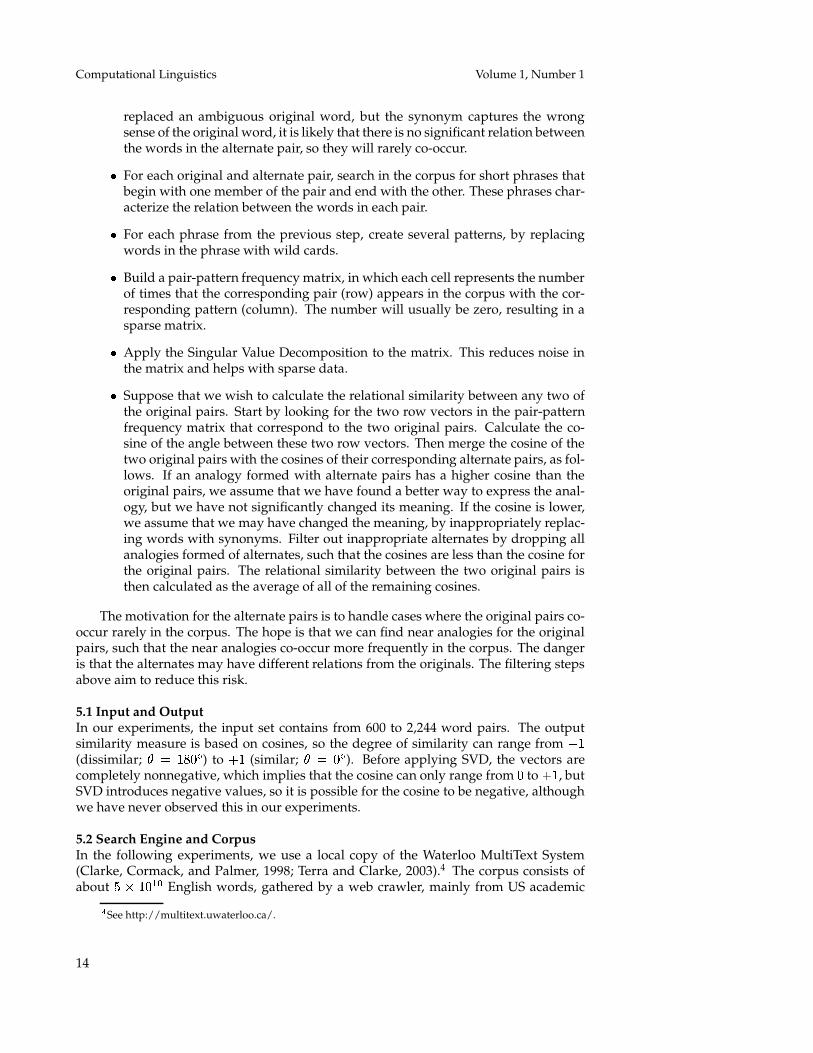
� Suppose that we wish to calculate the relational similarity between any two ofthe original pairs. Start by looking for the two row vectors in the pair-patternfrequency matrix that correspond to the two original pairs. Calculate the co-sine of the angle between these two row vectors. Then merge the cosine of thetwo original pairs with the cosines of their corresponding alternate pairs, as fol-lows. If an analogy formed with alternate pairs has a higher cosine than theoriginal pairs, we assume that we have found a better way to express the anal-ogy, but we have not significantly changed its meaning. If the cosine is lower,we assume that we may have changed the meaning, by inappropriately replac-ing words with synonyms. Filter out inappropriate alternates by dropping allanalogies formed of alternates, such that the cosines are less than the cosine forthe original pairs. The relational similarity between the two original pairs isthen calculated as the average of all of the remaining cosines.
The motivation for the alternate pairs is to handle cases where the original pairs co-occur rarely in the corpus. The hope is that we can find near analogies for the originalpairs, such that the near analogies co-occur more frequently in the corpus. The dangeris that the alternates may have different relations from the originals. The filtering stepsabove aim to reduce this risk.
5.1 Input and OutputIn our experiments, the input set contains from 600 to 2,244 word pairs. The outputsimilarity measure is based on cosines, so the degree of similarity can range from �
�
(dissimilar;�
� ����) to ��
(similar;�
� ��). Before applying SVD, the vectors are
completely nonnegative, which implies that the cosine can only range from�
to ��, but
SVD introduces negative values, so it is possible for the cosine to be negative, althoughwe have never observed this in our experiments.
5.2 Search Engine and CorpusIn the following experiments, we use a local copy of the Waterloo MultiText System(Clarke, Cormack, and Palmer, 1998; Terra and Clarke, 2003).4 The corpus consists ofabout � � �� �� English words, gathered by a web crawler, mainly from US academic
�See http://multitext.uwaterloo.ca/.
14
Similarity of Semantic Relations Turney
web sites. The web pages cover a very wide range of topics, styles, genres, quality, andwriting skill. The WMTS is well suited to LRA, because the WMTS scales well to largecorpora (one terabyte, in our case), it gives exact frequency counts (unlike most websearch engines), it is designed for passage retrieval (rather than document retrieval),and it has a powerful query syntax.
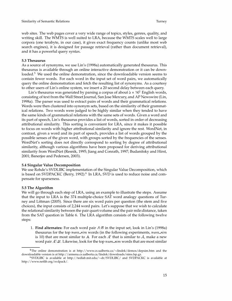
5.3 ThesaurusAs a source of synonyms, we use Lin’s (1998a) automatically generated thesaurus. Thisthesaurus is available through an online interactive demonstration or it can be down-loaded.5 We used the online demonstration, since the downloadable version seems tocontain fewer words. For each word in the input set of word pairs, we automaticallyquery the online demonstration and fetch the resulting list of synonyms. As a courtesyto other users of Lin’s online system, we insert a 20 second delay between each query.
Lin’s thesaurus was generated by parsing a corpus of about � � ���English words,
consisting of text from the Wall Street Journal, San Jose Mercury, and AP Newswire (Lin,1998a). The parser was used to extract pairs of words and their grammatical relations.Words were then clustered into synonym sets, based on the similarity of their grammat-ical relations. Two words were judged to be highly similar when they tended to havethe same kinds of grammatical relations with the same sets of words. Given a word andits part of speech, Lin’s thesaurus provides a list of words, sorted in order of decreasingattributional similarity. This sorting is convenient for LRA, since it makes it possibleto focus on words with higher attributional similarity and ignore the rest. WordNet, incontrast, given a word and its part of speech, provides a list of words grouped by thepossible senses of the given word, with groups sorted by the frequencies of the senses.WordNet’s sorting does not directly correspond to sorting by degree of attributionalsimilarity, although various algorithms have been proposed for deriving attributionalsimilarity from WordNet (Resnik, 1995; Jiang and Conrath, 1997; Budanitsky and Hirst,2001; Banerjee and Pedersen, 2003).
5.4 Singular Value DecompositionWe use Rohde’s SVDLIBC implementation of the Singular Value Decomposition, whichis based on SVDPACKC (Berry, 1992).6 In LRA, SVD is used to reduce noise and com-pensate for sparseness.
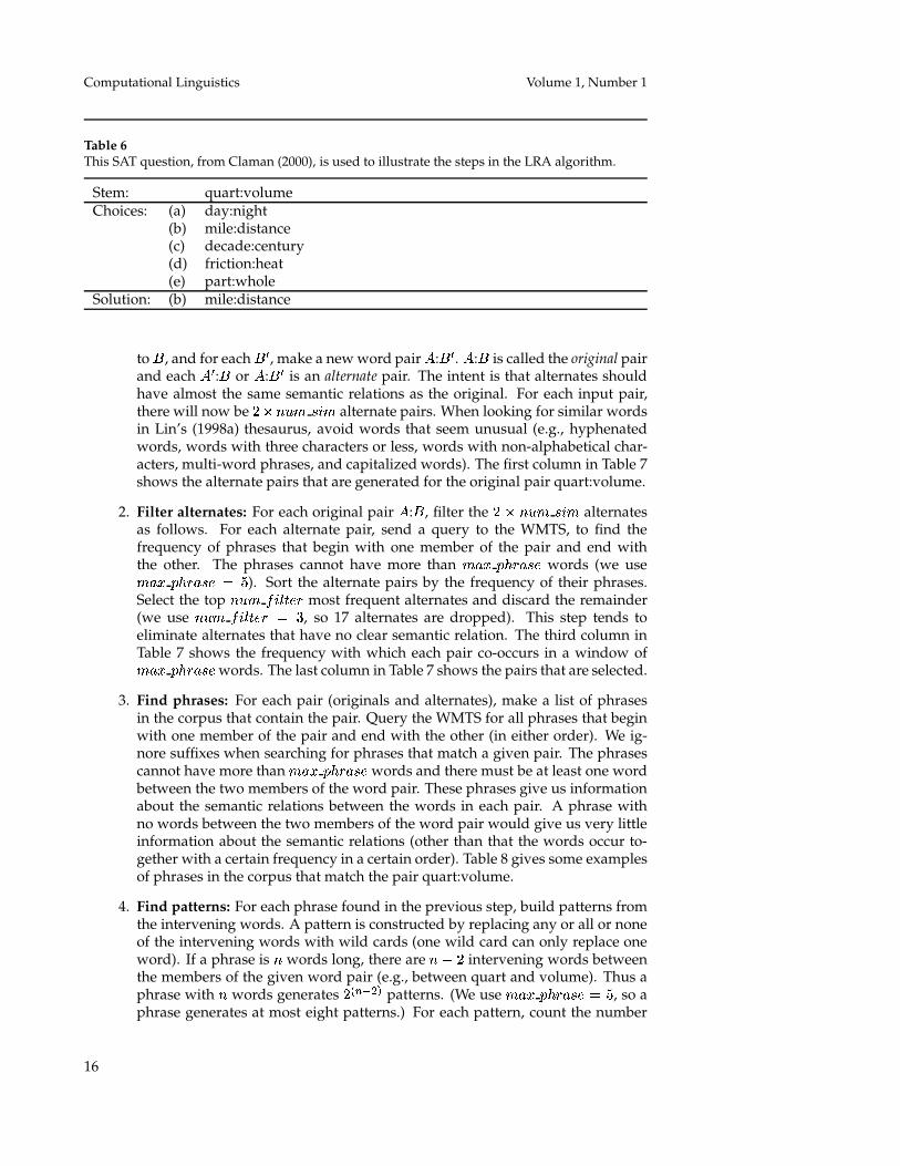
5.5 The AlgorithmWe will go through each step of LRA, using an example to illustrate the steps. Assumethat the input to LRA is the 374 multiple-choice SAT word analogy questions of Tur-ney and Littman (2005). Since there are six word pairs per question (the stem and fivechoices), the input consists of 2,244 word pairs. Let’s suppose that we wish to calculatethe relational similarity between the pair quart:volume and the pair mile:distance, takenfrom the SAT question in Table 6. The LRA algorithm consists of the following twelvesteps:
1. Find alternates: For each word pair � :� in the input set, look in Lin’s (1998a)thesaurus for the top ��� �
�� words (in the following experiments, ��� �
��
is 10) that are most similar to � . For each � � that is similar to � , make a newword pair � �:� . Likewise, look for the top ��� �
�� words that are most similar
�The online demonstration is at http://www.cs.ualberta.ca/�lindek/demos/depsim.htm and the
downloadable version is at http://armena.cs.ualberta.ca/lindek/downloads/sims.lsp.gz.�SVDLIBC is available at http://tedlab.mit.edu/�dr/SVDLIBC/ and SVDPACKC is available at
http://www.netlib.org/svdpack/.
15
Computational Linguistics Volume 1, Number 1
Table 6This SAT question, from Claman (2000), is used to illustrate the steps in the LRA algorithm.
Stem: quart:volumeChoices: (a) day:night
(b) mile:distance(c) decade:century(d) friction:heat(e) part:whole
Solution: (b) mile:distance
to � , and for each � �, make a new word pair � :� �. � :� is called the original pairand each � �:� or � :� � is an alternate pair. The intent is that alternates shouldhave almost the same semantic relations as the original. For each input pair,there will now be
� ���� �
�� alternate pairs. When looking for similar words
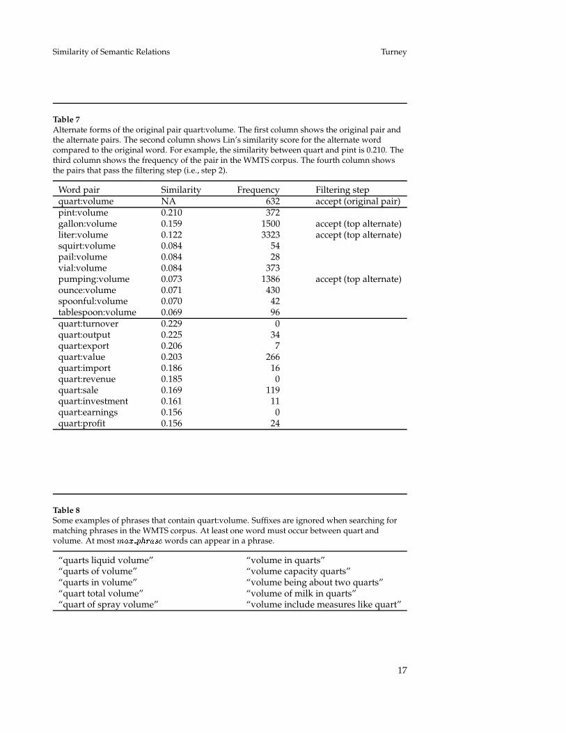
in Lin’s (1998a) thesaurus, avoid words that seem unusual (e.g., hyphenatedwords, words with three characters or less, words with non-alphabetical char-acters, multi-word phrases, and capitalized words). The first column in Table 7shows the alternate pairs that are generated for the original pair quart:volume.
2. Filter alternates: For each original pair � :� , filter the� �
��� ��� alternates
as follows. For each alternate pair, send a query to the WMTS, to find thefrequency of phrases that begin with one member of the pair and end withthe other. The phrases cannot have more than � �� � ����� words (we use� �� � ����� � �). Sort the alternate pairs by the frequency of their phrases.Select the top ��� � ����� most frequent alternates and discard the remainder(we use ��� � ����� � �, so 17 alternates are dropped). This step tends toeliminate alternates that have no clear semantic relation. The third column inTable 7 shows the frequency with which each pair co-occurs in a window of� �� � ����� words. The last column in Table 7 shows the pairs that are selected.
3. Find phrases: For each pair (originals and alternates), make a list of phrasesin the corpus that contain the pair. Query the WMTS for all phrases that beginwith one member of the pair and end with the other (in either order). We ig-nore suffixes when searching for phrases that match a given pair. The phrasescannot have more than � �� � ����� words and there must be at least one wordbetween the two members of the word pair. These phrases give us informationabout the semantic relations between the words in each pair. A phrase withno words between the two members of the word pair would give us very littleinformation about the semantic relations (other than that the words occur to-gether with a certain frequency in a certain order). Table 8 gives some examplesof phrases in the corpus that match the pair quart:volume.
4. Find patterns: For each phrase found in the previous step, build patterns fromthe intervening words. A pattern is constructed by replacing any or all or noneof the intervening words with wild cards (one wild card can only replace oneword). If a phrase is � words long, there are � �
�intervening words between
the members of the given word pair (e.g., between quart and volume). Thus aphrase with � words generates
� ���� patterns. (We use � �� � ����� � �, so aphrase generates at most eight patterns.) For each pattern, count the number
16
Similarity of Semantic Relations Turney
Table 7Alternate forms of the original pair quart:volume. The first column shows the original pair andthe alternate pairs. The second column shows Lin’s similarity score for the alternate wordcompared to the original word. For example, the similarity between quart and pint is 0.210. Thethird column shows the frequency of the pair in the WMTS corpus. The fourth column showsthe pairs that pass the filtering step (i.e., step 2).
Word pair Similarity Frequency Filtering stepquart:volume NA 632 accept (original pair)pint:volume 0.210 372gallon:volume 0.159 1500 accept (top alternate)liter:volume 0.122 3323 accept (top alternate)squirt:volume 0.084 54pail:volume 0.084 28vial:volume 0.084 373pumping:volume 0.073 1386 accept (top alternate)ounce:volume 0.071 430spoonful:volume 0.070 42tablespoon:volume 0.069 96quart:turnover 0.229 0quart:output 0.225 34quart:export 0.206 7quart:value 0.203 266quart:import 0.186 16quart:revenue 0.185 0quart:sale 0.169 119quart:investment 0.161 11quart:earnings 0.156 0quart:profit 0.156 24
Table 8Some examples of phrases that contain quart:volume. Suffixes are ignored when searching formatching phrases in the WMTS corpus. At least one word must occur between quart andvolume. At most ��� � ����� words can appear in a phrase.
“quarts liquid volume” “volume in quarts”“quarts of volume” “volume capacity quarts”“quarts in volume” “volume being about two quarts”“quart total volume” “volume of milk in quarts”“quart of spray volume” “volume include measures like quart”
17
Computational Linguistics Volume 1, Number 1
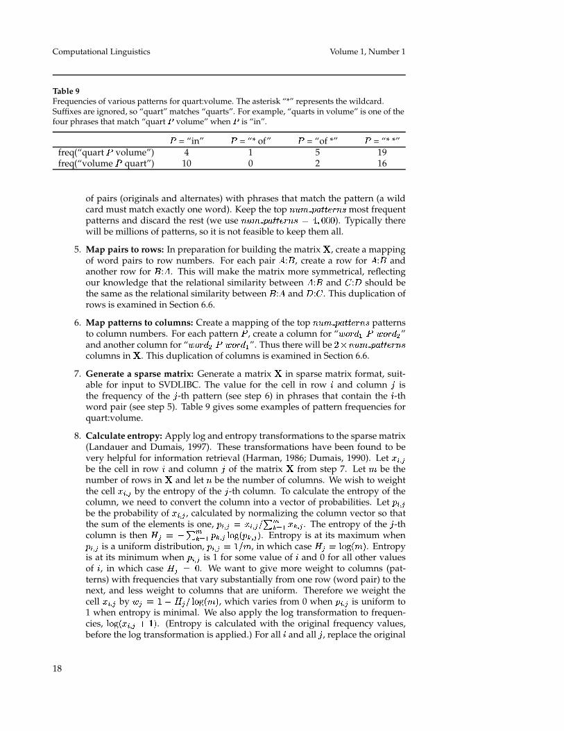
Table 9Frequencies of various patterns for quart:volume. The asterisk “*” represents the wildcard.Suffixes are ignored, so “quart” matches “quarts”. For example, “quarts in volume” is one of thefour phrases that match “quart � volume” when � is “in”.
�= “in”
�= “* of”
�= “of *”
�= “* *”
freq(“quart�
volume”) 4 1 5 19freq(“volume
�quart”) 10 0 2 16
of pairs (originals and alternates) with phrases that match the pattern (a wildcard must match exactly one word). Keep the top ��� � ������� most frequentpatterns and discard the rest (we use ��� � ������� � � � ���). Typically therewill be millions of patterns, so it is not feasible to keep them all.
5. Map pairs to rows: In preparation for building the matrix � , create a mappingof word pairs to row numbers. For each pair � :� , create a row for � :� andanother row for � :� . This will make the matrix more symmetrical, reflectingour knowledge that the relational similarity between � :� and � :� should bethe same as the relational similarity between � :� and � :� . This duplication ofrows is examined in Section 6.6.
6. Map patterns to columns: Create a mapping of the top ��� � ������� patternsto column numbers. For each pattern
�, create a column for “� ��� � � � ����”
and another column for “� ���� � � ��� �”. Thus there will be� �
��� � �������columns in � . This duplication of columns is examined in Section 6.6.
7. Generate a sparse matrix: Generate a matrix � in sparse matrix format, suit-able for input to SVDLIBC. The value for the cell in row
�and column � is
the frequency of the � -th pattern (see step 6) in phrases that contain the�-th
word pair (see step 5). Table 9 gives some examples of pattern frequencies forquart:volume.
8. Calculate entropy: Apply log and entropy transformations to the sparse matrix(Landauer and Dumais, 1997). These transformations have been found to bevery helpful for information retrieval (Harman, 1986; Dumais, 1990). Let � ��be the cell in row
�and column � of the matrix � from step 7. Let � be the
number of rows in � and let � be the number of columns. We wish to weightthe cell � �� by the entropy of the � -th column. To calculate the entropy of thecolumn, we need to convert the column into a vector of probabilities. Let � ��be the probability of � �� , calculated by normalizing the column vector so thatthe sum of the elements is one, � �� � � �� ���� � �� . The entropy of the � -thcolumn is then � � �
��� � �� ��� � �� �. Entropy is at its maximum when� �� is a uniform distribution, � �� � ��
� , in which case � � ��� � �. Entropyis at its minimum when � �� is 1 for some value of
�and 0 for all other values
of�, in which case � � �
. We want to give more weight to columns (pat-terns) with frequencies that vary substantially from one row (word pair) to thenext, and less weight to columns that are uniform. Therefore we weight thecell � �� by �� � �
� � � ��� � �, which varies from 0 when � �� is uniform to1 when entropy is minimal. We also apply the log transformation to frequen-cies, ��� � �� � ��. (Entropy is calculated with the original frequency values,before the log transformation is applied.) For all
�and all � , replace the original
18
Similarity of Semantic Relations Turney
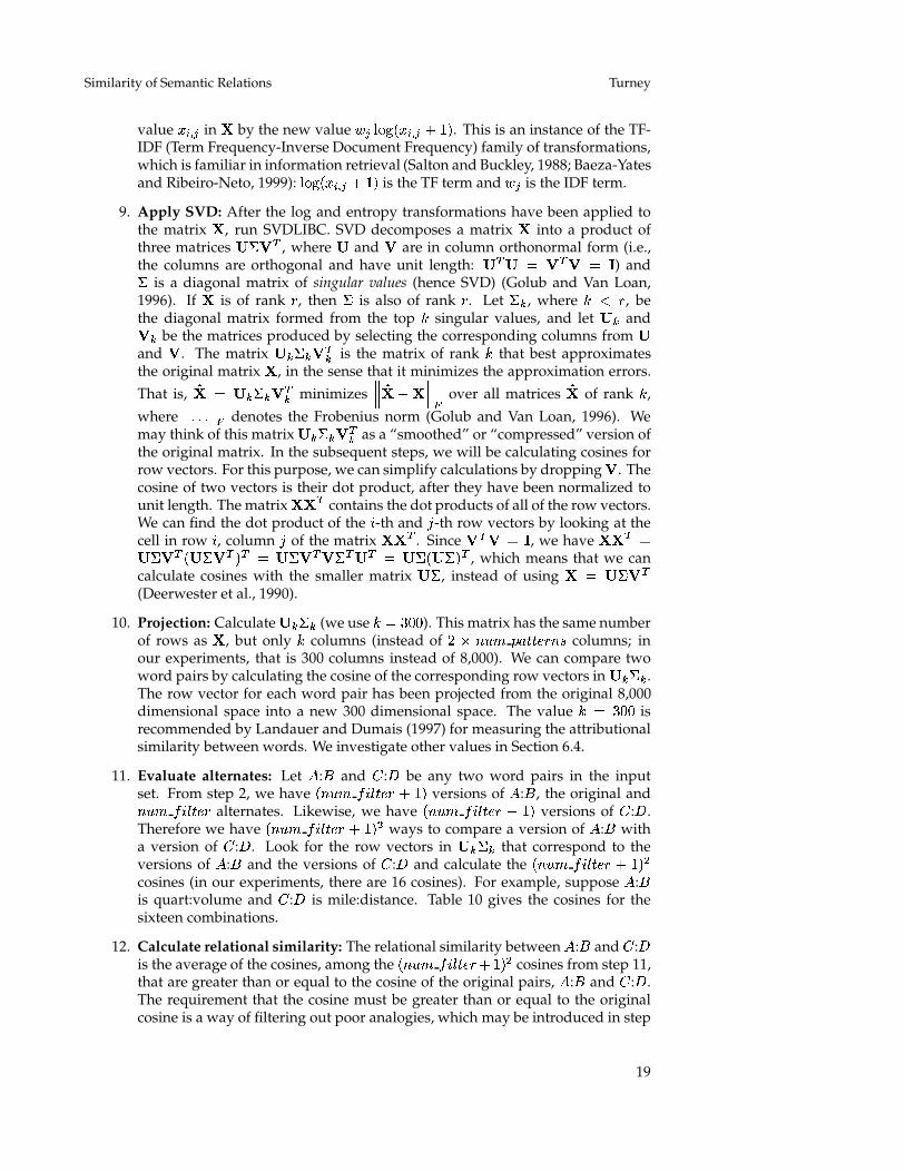
value � �� in � by the new value �� ��� � �� � ��. This is an instance of the TF-IDF (Term Frequency-Inverse Document Frequency) family of transformations,which is familiar in information retrieval (Salton and Buckley, 1988; Baeza-Yatesand Ribeiro-Neto, 1999): ��� � �� � �� is the TF term and �� is the IDF term.
9. Apply SVD: After the log and entropy transformations have been applied tothe matrix � , run SVDLIBC. SVD decomposes a matrix � into a product ofthree matrices ��� � , where � and � are in column orthonormal form (i.e.,the columns are orthogonal and have unit length: �� � � �� � � �) and� is a diagonal matrix of singular values (hence SVD) (Golub and Van Loan,1996). If � is of rank �, then � is also of rank � . Let � , where � � � , bethe diagonal matrix formed from the top � singular values, and let � and� be the matrices produced by selecting the corresponding columns from �and � . The matrix � � � � is the matrix of rank � that best approximatesthe original matrix � , in the sense that it minimizes the approximation errors.
That is,�� � � � �� minimizes
����� � �
��� over all matrices�� of rank � ,
where�� � �� denotes the Frobenius norm (Golub and Van Loan, 1996). We
may think of this matrix � � � � as a “smoothed” or “compressed” version ofthe original matrix. In the subsequent steps, we will be calculating cosines forrow vectors. For this purpose, we can simplify calculations by dropping � . Thecosine of two vectors is their dot product, after they have been normalized tounit length. The matrix �� � contains the dot products of all of the row vectors.We can find the dot product of the
�-th and � -th row vectors by looking at the
cell in row�, column � of the matrix �� � . Since � � � � �, we have �� � �
��� � ���� �� � ��� � � �� �� � �� �� �� , which means that we cancalculate cosines with the smaller matrix ��, instead of using � � ��� �(Deerwester et al., 1990).
10. Projection: Calculate � � (we use � � ���). This matrix has the same numberof rows as � , but only � columns (instead of
� ���� � ������� columns; in
our experiments, that is 300 columns instead of 8,000). We can compare twoword pairs by calculating the cosine of the corresponding row vectors in � � .The row vector for each word pair has been projected from the original 8,000dimensional space into a new 300 dimensional space. The value � � ��� isrecommended by Landauer and Dumais (1997) for measuring the attributionalsimilarity between words. We investigate other values in Section 6.4.
11. Evaluate alternates: Let � :� and � :� be any two word pairs in the inputset. From step 2, we have ��� � ����� � �� versions of � :� , the original and��� � ����� alternates. Likewise, we have ��� � ����� � �� versions of � :� .Therefore we have ��� � ����� � ��� ways to compare a version of � :� witha version of � :� . Look for the row vectors in � � that correspond to theversions of � :� and the versions of � :� and calculate the ��� � ����� � ���cosines (in our experiments, there are 16 cosines). For example, suppose � :�is quart:volume and � :� is mile:distance. Table 10 gives the cosines for thesixteen combinations.
12. Calculate relational similarity: The relational similarity between � :� and � :�is the average of the cosines, among the ��� � ����� � ��� cosines from step 11,that are greater than or equal to the cosine of the original pairs, � :� and � :� .The requirement that the cosine must be greater than or equal to the originalcosine is a way of filtering out poor analogies, which may be introduced in step
19
Computational Linguistics Volume 1, Number 1
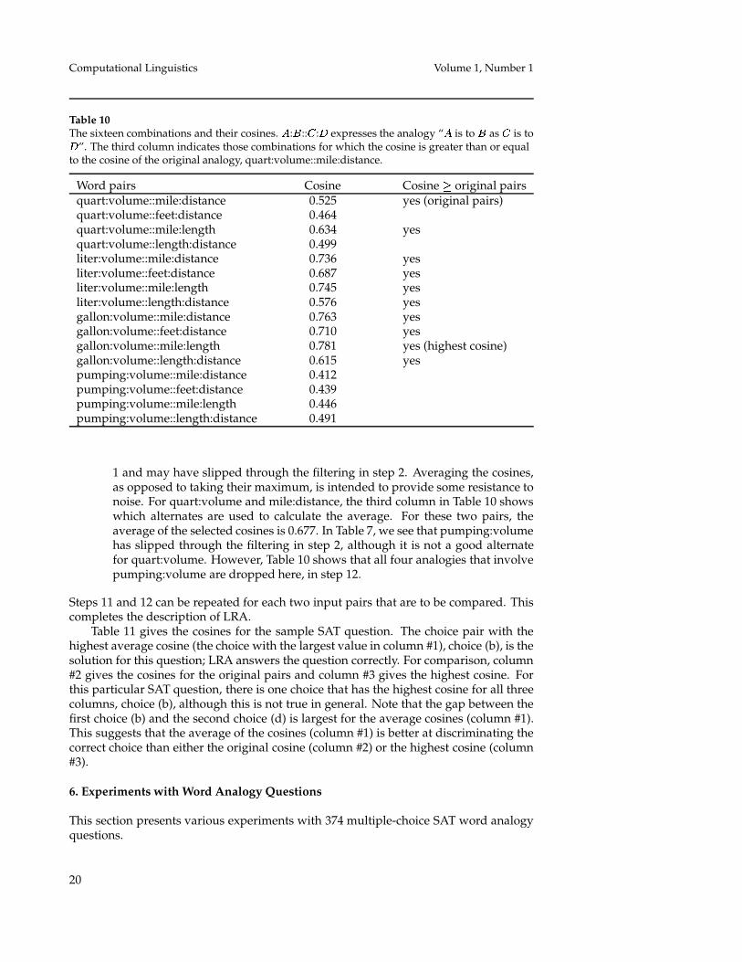
Table 10The sixteen combinations and their cosines. � :� ::� :� expresses the analogy “� is to � as � is to�”. The third column indicates those combinations for which the cosine is greater than or equalto the cosine of the original analogy, quart:volume::mile:distance.
Word pairs Cosine Cosine � original pairsquart:volume::mile:distance 0.525 yes (original pairs)quart:volume::feet:distance 0.464quart:volume::mile:length 0.634 yesquart:volume::length:distance 0.499liter:volume::mile:distance 0.736 yesliter:volume::feet:distance 0.687 yesliter:volume::mile:length 0.745 yesliter:volume::length:distance 0.576 yesgallon:volume::mile:distance 0.763 yesgallon:volume::feet:distance 0.710 yesgallon:volume::mile:length 0.781 yes (highest cosine)gallon:volume::length:distance 0.615 yespumping:volume::mile:distance 0.412pumping:volume::feet:distance 0.439pumping:volume::mile:length 0.446pumping:volume::length:distance 0.491
1 and may have slipped through the filtering in step 2. Averaging the cosines,as opposed to taking their maximum, is intended to provide some resistance tonoise. For quart:volume and mile:distance, the third column in Table 10 showswhich alternates are used to calculate the average. For these two pairs, theaverage of the selected cosines is 0.677. In Table 7, we see that pumping:volumehas slipped through the filtering in step 2, although it is not a good alternatefor quart:volume. However, Table 10 shows that all four analogies that involvepumping:volume are dropped here, in step 12.
Steps 11 and 12 can be repeated for each two input pairs that are to be compared. Thiscompletes the description of LRA.
Table 11 gives the cosines for the sample SAT question. The choice pair with thehighest average cosine (the choice with the largest value in column #1), choice (b), is thesolution for this question; LRA answers the question correctly. For comparison, column#2 gives the cosines for the original pairs and column #3 gives the highest cosine. Forthis particular SAT question, there is one choice that has the highest cosine for all threecolumns, choice (b), although this is not true in general. Note that the gap between thefirst choice (b) and the second choice (d) is largest for the average cosines (column #1).This suggests that the average of the cosines (column #1) is better at discriminating thecorrect choice than either the original cosine (column #2) or the highest cosine (column#3).
6. Experiments with Word Analogy Questions
This section presents various experiments with 374 multiple-choice SAT word analogyquestions.
20

Similarity of Semantic Relations Turney
Table 11Cosines for the sample SAT question given in Table 6. Column #1 gives the averages of thecosines that are greater than or equal to the original cosines (e.g., the average of the cosines thatare marked “yes” in Table 10 is 0.677; see choice (b) in column #1). Column #2 gives the cosinefor the original pairs (e.g., the cosine for the first pair in Table 10 is 0.525; see choice (b) in column#2). Column #3 gives the maximum cosine for the sixteen possible analogies (e.g., the maximumcosine in Table 10 is 0.781; see choice (b) in column #3).
Average Original Highestcosines cosines cosines
Stem: quart:volume #1 #2 #3Choices: (a) day:night 0.374 0.327 0.443
(b) mile:distance 0.677 0.525 0.781(c) decade:century 0.389 0.327 0.470(d) friction:heat 0.428 0.336 0.552(e) part:whole 0.370 0.330 0.408
Solution: (b) mile:distance 0.677 0.525 0.781Gap: (b)-(d) 0.249 0.189 0.229
Table 12Performance of LRA on the 374 SAT questions. Precision, recall, and
�are reported as
percentages. (The bottom five rows are included for comparison.)
Algorithm Precision Recall �LRA 56.8 56.1 56.5Veale (2004) 42.8 42.8 42.8best attributional similarity 35.0 35.0 35.0random guessing 20.0 20.0 20.0lowest co-occurrence frequency 16.8 16.8 16.8highest co-occurrence frequency 11.8 11.8 11.8
6.1 Baseline LRA SystemTable 12 shows the performance of the baseline LRA system on the 374 SAT questions,using the parameter settings and configuration described in Section 5. LRA correctlyanswered 210 of the 374 questions. 160 questions were answered incorrectly and 4 ques-tions were skipped, because the stem pair and its alternates were represented by zerovectors. The performance of LRA is significantly better than the lexicon-based approachof Veale (2004) (see Section 3.1) and the best performance using attributional similarity(see Section 2.3), with 95% confidence, according to the Fisher Exact Test (Agresti, 1990).
As another point of reference, consider the simple strategy of always guessing thechoice with the highest co-occurrence frequency. The idea here is that the words inthe solution pair may occur together frequently, because there is presumably a clearand meaningful relation between the solution words, whereas the distractors may onlyoccur together rarely, because they have no meaningful relation. This strategy is signif-cantly worse than random guessing. The opposite strategy, always guessing the choicepair with the lowest co-occurrence frequency, is also worse than random guessing (butnot significantly). It appears that the designers of the SAT questions deliberately chosedistractors that would thwart these two strategies.
21
Computational Linguistics Volume 1, Number 1
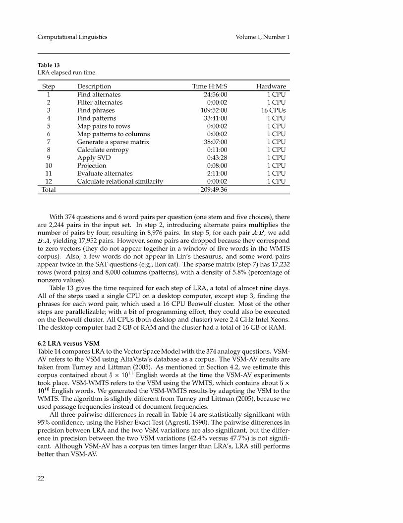
Table 13LRA elapsed run time.
Step Description Time H:M:S Hardware1 Find alternates 24:56:00 1 CPU2 Filter alternates 0:00:02 1 CPU3 Find phrases 109:52:00 16 CPUs4 Find patterns 33:41:00 1 CPU5 Map pairs to rows 0:00:02 1 CPU6 Map patterns to columns 0:00:02 1 CPU7 Generate a sparse matrix 38:07:00 1 CPU8 Calculate entropy 0:11:00 1 CPU9 Apply SVD 0:43:28 1 CPU
10 Projection 0:08:00 1 CPU11 Evaluate alternates 2:11:00 1 CPU12 Calculate relational similarity 0:00:02 1 CPU
Total 209:49:36
With 374 questions and 6 word pairs per question (one stem and five choices), thereare 2,244 pairs in the input set. In step 2, introducing alternate pairs multiplies thenumber of pairs by four, resulting in 8,976 pairs. In step 5, for each pair � :� , we add� :� , yielding 17,952 pairs. However, some pairs are dropped because they correspondto zero vectors (they do not appear together in a window of five words in the WMTScorpus). Also, a few words do not appear in Lin’s thesaurus, and some word pairsappear twice in the SAT questions (e.g., lion:cat). The sparse matrix (step 7) has 17,232rows (word pairs) and 8,000 columns (patterns), with a density of 5.8% (percentage ofnonzero values).
Table 13 gives the time required for each step of LRA, a total of almost nine days.All of the steps used a single CPU on a desktop computer, except step 3, finding thephrases for each word pair, which used a 16 CPU Beowulf cluster. Most of the othersteps are parallelizable; with a bit of programming effort, they could also be executedon the Beowulf cluster. All CPUs (both desktop and cluster) were 2.4 GHz Intel Xeons.The desktop computer had 2 GB of RAM and the cluster had a total of 16 GB of RAM.
6.2 LRA versus VSMTable 14 compares LRA to the Vector Space Model with the 374 analogy questions. VSM-AV refers to the VSM using AltaVista’s database as a corpus. The VSM-AV results aretaken from Turney and Littman (2005). As mentioned in Section 4.2, we estimate thiscorpus contained about � � �� �� English words at the time the VSM-AV experimentstook place. VSM-WMTS refers to the VSM using the WMTS, which contains about � ��� �� English words. We generated the VSM-WMTS results by adapting the VSM to theWMTS. The algorithm is slightly different from Turney and Littman (2005), because weused passage frequencies instead of document frequencies.
All three pairwise differences in recall in Table 14 are statistically significant with95% confidence, using the Fisher Exact Test (Agresti, 1990). The pairwise differences inprecision between LRA and the two VSM variations are also significant, but the differ-ence in precision between the two VSM variations (42.4% versus 47.7%) is not signifi-cant. Although VSM-AV has a corpus ten times larger than LRA’s, LRA still performsbetter than VSM-AV.
22
Similarity of Semantic Relations Turney
Table 14LRA versus VSM with 374 SAT analogy questions.
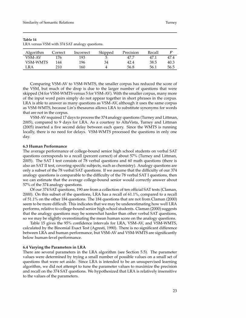
Algorithm Correct Incorrect Skipped Precision Recall �VSM-AV 176 193 5 47.7 47.1 47.4VSM-WMTS 144 196 34 42.4 38.5 40.3LRA 210 160 4 56.8 56.1 56.5
Comparing VSM-AV to VSM-WMTS, the smaller corpus has reduced the score ofthe VSM, but much of the drop is due to the larger number of questions that wereskipped (34 for VSM-WMTS versus 5 for VSM-AV). With the smaller corpus, many moreof the input word pairs simply do not appear together in short phrases in the corpus.LRA is able to answer as many questions as VSM-AV, although it uses the same corpusas VSM-WMTS, because Lin’s thesaurus allows LRA to substitute synonyms for wordsthat are not in the corpus.
VSM-AV required 17 days to process the 374 analogy questions (Turney and Littman,2005), compared to 9 days for LRA. As a courtesy to AltaVista, Turney and Littman(2005) inserted a five second delay between each query. Since the WMTS is runninglocally, there is no need for delays. VSM-WMTS processed the questions in only oneday.
6.3 Human PerformanceThe average performance of college-bound senior high school students on verbal SATquestions corresponds to a recall (percent correct) of about 57% (Turney and Littman,2005). The SAT I test consists of 78 verbal questions and 60 math questions (there isalso an SAT II test, covering specific subjects, such as chemistry). Analogy questions areonly a subset of the 78 verbal SAT questions. If we assume that the difficulty of our 374analogy questions is comparable to the difficulty of the 78 verbal SAT I questions, thenwe can estimate that the average college-bound senior would correctly answer about57% of the 374 analogy questions.
Of our 374 SAT questions, 190 are from a collection of ten official SAT tests (Claman,2000). On this subset of the questions, LRA has a recall of 61.1%, compared to a recallof 51.1% on the other 184 questions. The 184 questions that are not from Claman (2000)seem to be more difficult. This indicates that we may be underestimating how well LRAperforms, relative to college-bound senior high school students. Claman (2000) suggeststhat the analogy questions may be somewhat harder than other verbal SAT questions,so we may be slightly overestimating the mean human score on the analogy questions.
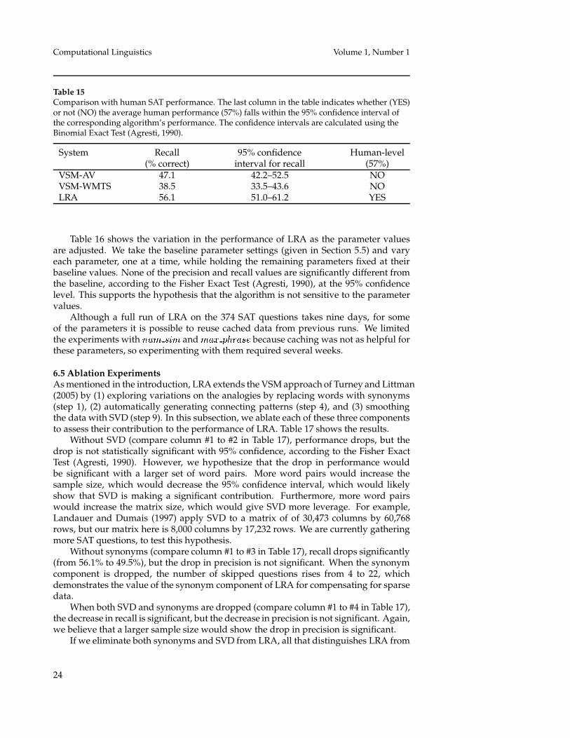
Table 15 gives the 95% confidence intervals for LRA, VSM-AV, and VSM-WMTS,calculated by the Binomial Exact Test (Agresti, 1990). There is no significant differencebetween LRA and human performance, but VSM-AV and VSM-WMTS are significantlybelow human-level performance.
6.4 Varying the Parameters in LRAThere are several parameters in the LRA algorithm (see Section 5.5). The parametervalues were determined by trying a small number of possible values on a small set ofquestions that were set aside. Since LRA is intended to be an unsupervised learningalgorithm, we did not attempt to tune the parameter values to maximize the precisionand recall on the 374 SAT questions. We hypothesized that LRA is relatively insensitiveto the values of the parameters.
23
Computational Linguistics Volume 1, Number 1
Table 15Comparison with human SAT performance. The last column in the table indicates whether (YES)or not (NO) the average human performance (57%) falls within the 95% confidence interval ofthe corresponding algorithm’s performance. The confidence intervals are calculated using theBinomial Exact Test (Agresti, 1990).
System Recall 95% confidence Human-level(% correct) interval for recall (57%)
VSM-AV 47.1 42.2–52.5 NOVSM-WMTS 38.5 33.5–43.6 NOLRA 56.1 51.0–61.2 YES
Table 16 shows the variation in the performance of LRA as the parameter valuesare adjusted. We take the baseline parameter settings (given in Section 5.5) and varyeach parameter, one at a time, while holding the remaining parameters fixed at theirbaseline values. None of the precision and recall values are significantly different fromthe baseline, according to the Fisher Exact Test (Agresti, 1990), at the 95% confidencelevel. This supports the hypothesis that the algorithm is not sensitive to the parametervalues.
Although a full run of LRA on the 374 SAT questions takes nine days, for someof the parameters it is possible to reuse cached data from previous runs. We limitedthe experiments with ��� �
�� and � �� � ����� because caching was not as helpful for
these parameters, so experimenting with them required several weeks.
6.5 Ablation ExperimentsAs mentioned in the introduction, LRA extends the VSM approach of Turney and Littman(2005) by (1) exploring variations on the analogies by replacing words with synonyms(step 1), (2) automatically generating connecting patterns (step 4), and (3) smoothingthe data with SVD (step 9). In this subsection, we ablate each of these three componentsto assess their contribution to the performance of LRA. Table 17 shows the results.
Without SVD (compare column #1 to #2 in Table 17), performance drops, but thedrop is not statistically significant with 95% confidence, according to the Fisher ExactTest (Agresti, 1990). However, we hypothesize that the drop in performance wouldbe significant with a larger set of word pairs. More word pairs would increase thesample size, which would decrease the 95% confidence interval, which would likelyshow that SVD is making a significant contribution. Furthermore, more word pairswould increase the matrix size, which would give SVD more leverage. For example,Landauer and Dumais (1997) apply SVD to a matrix of of 30,473 columns by 60,768rows, but our matrix here is 8,000 columns by 17,232 rows. We are currently gatheringmore SAT questions, to test this hypothesis.
Without synonyms (compare column #1 to #3 in Table 17), recall drops significantly(from 56.1% to 49.5%), but the drop in precision is not significant. When the synonymcomponent is dropped, the number of skipped questions rises from 4 to 22, whichdemonstrates the value of the synonym component of LRA for compensating for sparsedata.
When both SVD and synonyms are dropped (compare column #1 to #4 in Table 17),the decrease in recall is significant, but the decrease in precision is not significant. Again,we believe that a larger sample size would show the drop in precision is significant.
If we eliminate both synonyms and SVD from LRA, all that distinguishes LRA from
24

Similarity of Semantic Relations Turney
Table 16Variation in performance with different parameter values. The Baseline column marks thebaseline parameter values. The Step column gives the step number in Section 5.5 where eachparameter is discussed.
Parameter Baseline Value Step Precision Recall ���� �
�� 5 1 54.2 53.5 53.8
��� ��� � 10 1 56.8 56.1 56.5
��� ��� 15 1 54.1 53.5 53.8
� �� � ����� 4 2 55.8 55.1 55.5� �� � ����� � 5 2 56.8 56.1 56.5� �� � ����� 6 2 56.2 55.6 55.9��� � ����� 1 2 54.3 53.7 54.0��� � ����� 2 2 55.7 55.1 55.4��� � ����� � 3 2 56.8 56.1 56.5��� � ����� 4 2 55.7 55.1 55.4��� � ����� 5 2 54.3 53.7 54.0
��� � ������� 1000 4 55.9 55.3 55.6��� � ������� 2000 4 57.6 57.0 57.3��� � ������� 3000 4 58.4 57.8 58.1��� � ������� � 4000 4 56.8 56.1 56.5��� � ������� 5000 4 57.0 56.4 56.7��� � ������� 6000 4 57.0 56.4 56.7��� � ������� 7000 4 58.1 57.5 57.8
� 100 10 55.7 55.1 55.4� � 300 10 56.8 56.1 56.5� 500 10 57.6 57.0 57.3� 700 10 56.5 55.9 56.2� 900 10 56.2 55.6 55.9
Table 17Results of ablation experiments.
LRA LRAbaseline LRA LRA no SVDsystem no SVD no synonyms no synonyms VSM-WMTS
#1 #2 #3 #4 #5Correct 210 198 185 178 144Incorrect 160 172 167 173 196Skipped 4 4 22 23 34Precision 56.8 53.5 52.6 50.7 42.4Recall 56.1 52.9 49.5 47.6 38.5� 56.5 53.2 51.0 49.1 40.3
25
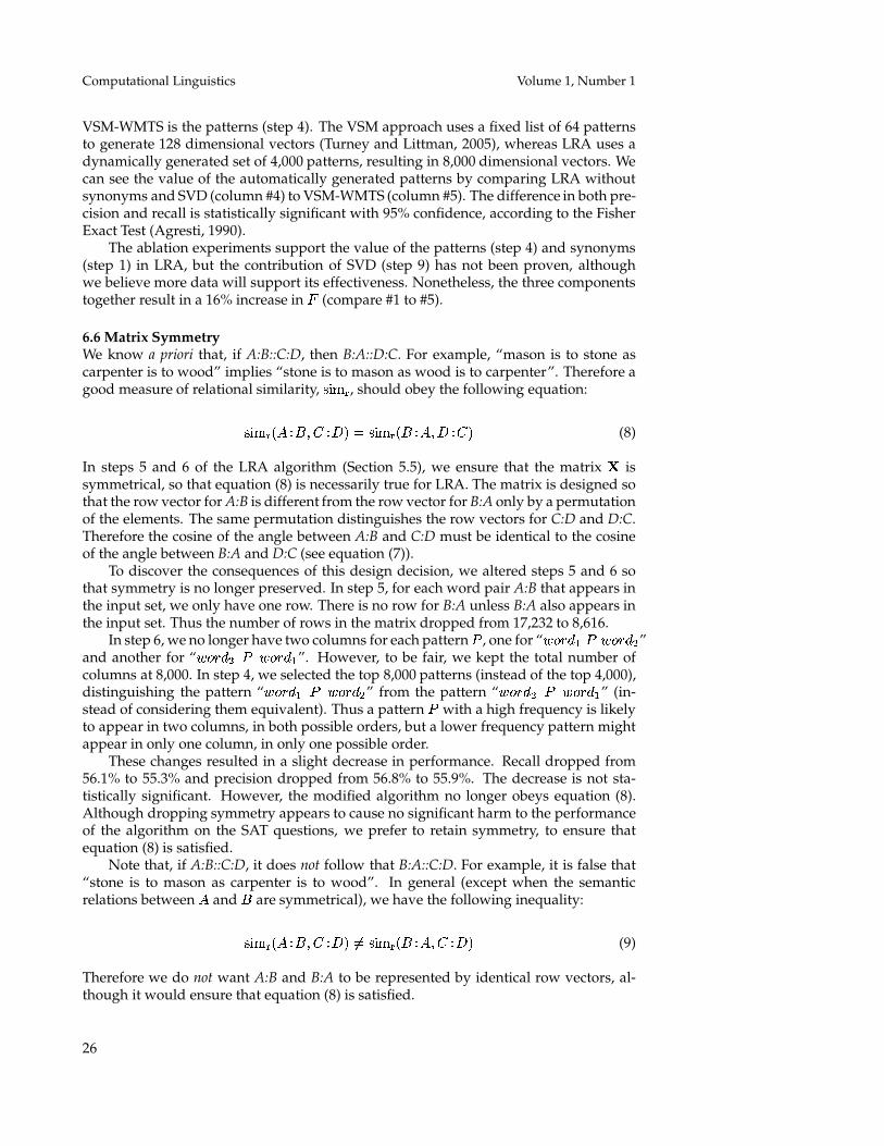
Computational Linguistics Volume 1, Number 1
VSM-WMTS is the patterns (step 4). The VSM approach uses a fixed list of 64 patternsto generate 128 dimensional vectors (Turney and Littman, 2005), whereas LRA uses adynamically generated set of 4,000 patterns, resulting in 8,000 dimensional vectors. Wecan see the value of the automatically generated patterns by comparing LRA withoutsynonyms and SVD (column #4) to VSM-WMTS (column #5). The difference in both pre-cision and recall is statistically significant with 95% confidence, according to the FisherExact Test (Agresti, 1990).
The ablation experiments support the value of the patterns (step 4) and synonyms(step 1) in LRA, but the contribution of SVD (step 9) has not been proven, althoughwe believe more data will support its effectiveness. Nonetheless, the three componentstogether result in a 16% increase in � (compare #1 to #5).
6.6 Matrix SymmetryWe know a priori that, if A:B::C:D, then B:A::D:C. For example, “mason is to stone ascarpenter is to wood” implies “stone is to mason as wood is to carpenter”. Therefore agood measure of relational similarity, ��� � , should obey the following equation:
��� � � �� � � �� � � ��� � � �� � � �� � (8)
In steps 5 and 6 of the LRA algorithm (Section 5.5), we ensure that the matrix � issymmetrical, so that equation (8) is necessarily true for LRA. The matrix is designed sothat the row vector for A:B is different from the row vector for B:A only by a permutationof the elements. The same permutation distinguishes the row vectors for C:D and D:C.Therefore the cosine of the angle between A:B and C:D must be identical to the cosineof the angle between B:A and D:C (see equation (7)).
To discover the consequences of this design decision, we altered steps 5 and 6 sothat symmetry is no longer preserved. In step 5, for each word pair A:B that appears inthe input set, we only have one row. There is no row for B:A unless B:A also appears inthe input set. Thus the number of rows in the matrix dropped from 17,232 to 8,616.
In step 6, we no longer have two columns for each pattern�
, one for “� ��� � � � ����”and another for “� ���� � � ��� �”. However, to be fair, we kept the total number ofcolumns at 8,000. In step 4, we selected the top 8,000 patterns (instead of the top 4,000),distinguishing the pattern “� ��� � � � ����” from the pattern “� ���� � � ��� �” (in-stead of considering them equivalent). Thus a pattern
�with a high frequency is likely
to appear in two columns, in both possible orders, but a lower frequency pattern mightappear in only one column, in only one possible order.
These changes resulted in a slight decrease in performance. Recall dropped from56.1% to 55.3% and precision dropped from 56.8% to 55.9%. The decrease is not sta-tistically significant. However, the modified algorithm no longer obeys equation (8).Although dropping symmetry appears to cause no significant harm to the performanceof the algorithm on the SAT questions, we prefer to retain symmetry, to ensure thatequation (8) is satisfied.
Note that, if A:B::C:D, it does not follow that B:A::C:D. For example, it is false that“stone is to mason as carpenter is to wood”. In general (except when the semanticrelations between � and � are symmetrical), we have the following inequality:
��� � � �� � � �� � �� ��� � � �� � � �� � (9)
Therefore we do not want A:B and B:A to be represented by identical row vectors, al-though it would ensure that equation (8) is satisfied.
26
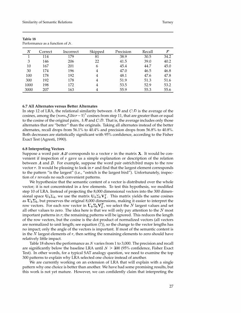
Similarity of Semantic Relations Turney
Table 18Performance as a function of � .
�Correct Incorrect Skipped Precision Recall �
1 114 179 81 38.9 30.5 34.23 146 206 22 41.5 39.0 40.2
10 167 201 6 45.4 44.7 45.030 174 196 4 47.0 46.5 46.8
100 178 192 4 48.1 47.6 47.8300 192 178 4 51.9 51.3 51.6
1000 198 172 4 53.5 52.9 53.23000 207 163 4 55.9 55.3 55.6
6.7 All Alternates versus Better AlternatesIn step 12 of LRA, the relational similarity between � :� and � :� is the average of thecosines, among the ��� � ����� � ��� cosines from step 11, that are greater than or equalto the cosine of the original pairs, � :� and � :� . That is, the average includes only thosealternates that are “better” than the originals. Taking all alternates instead of the betteralternates, recall drops from 56.1% to 40.4% and precision drops from 56.8% to 40.8%.Both decreases are statistically significant with 95% confidence, according to the FisherExact Test (Agresti, 1990).
6.8 Interpreting VectorsSuppose a word pair � :� corresponds to a vector � in the matrix � . It would be con-venient if inspection of � gave us a simple explanation or description of the relationbetween � and � . For example, suppose the word pair ostrich:bird maps to the rowvector � . It would be pleasing to look in � and find that the largest element correspondsto the pattern “is the largest” (i.e., “ostrich is the largest bird”). Unfortunately, inspec-tion of � reveals no such convenient patterns.
We hypothesize that the semantic content of a vector is distributed over the wholevector; it is not concentrated in a few elements. To test this hypothesis, we modifiedstep 10 of LRA. Instead of projecting the 8,000 dimensional vectors into the 300 dimen-sional space � � , we use the matrix � � �� . This matrix yields the same cosinesas � � , but preserves the original 8,000 dimensions, making it easier to interpret therow vectors. For each row vector in � � �� , we select the
�largest values and set
all other values to zero. The idea here is that we will only pay attention to the�
mostimportant patterns in � ; the remaining patterns will be ignored. This reduces the lengthof the row vectors, but the cosine is the dot product of normalized vectors (all vectorsare normalized to unit length; see equation (7)), so the change to the vector lengths hasno impact; only the angle of the vectors is important. If most of the semantic content isin the
�largest elements of � , then setting the remaining elements to zero should have
relatively little impact.Table 18 shows the performance as
�varies from 1 to 3,000. The precision and recall
are significantly below the baseline LRA until� � ��� (95% confidence, Fisher Exact
Test). In other words, for a typical SAT analogy question, we need to examine the top300 patterns to explain why LRA selected one choice instead of another.
We are currently working on an extension of LRA that will explain with a singlepattern why one choice is better than another. We have had some promising results, butthis work is not yet mature. However, we can confidently claim that interpreting the
27
Computational Linguistics Volume 1, Number 1
vectors is not trivial.
6.9 Manual Patterns versus Automatic PatternsTurney and Littman (2005) used 64 manually generated patterns whereas LRA uses4,000 automatically generated patterns. We know from Section 6.5 that the automati-cally generated patterns are significantly better than the manually generated patterns.It may be interesting to see how many of the manually generated patterns appear withinthe automatically generated patterns. If we require an exact match, 50 of the 64 manualpatterns can be found in the automatic patterns. If we are lenient about wildcards, andcount the pattern “not the” as matching “* not the” (for example), then 60 of the 64 man-ual patterns appear within the automatic patterns. This suggests that the improvementin performance with the automatic patterns is due to the increased quantity of patterns,rather than a qualitative difference in the patterns.
Turney and Littman (2005) point out that some of their 64 patterns have been usedby other researchers. For example, Hearst (1992) used the pattern “such as” to dis-cover hyponyms and Berland and Charniak (1999) used the pattern “of the” to discovermeronyms. Both of these patterns are included in the 4,000 patterns automatically gen-erated by LRA.
The novelty in Turney and Littman (2005) is that their patterns are not used to minetext for instances of word pairs that fit the patterns (Hearst, 1992; Berland and Charniak,1999); instead, they are used to gather frequency data for building vectors that representthe relation between a given pair of words. The results in Section 6.8 show that a vectorcontains more information than any single pattern or small set of patterns; a vector isa distributed representation. LRA is distinct from Hearst (1992) and Berland and Char-niak (1999) in its focus on distributed representations, which it shares with Turney andLittman (2005), but LRA goes beyond Turney and Littman (2005) by finding patternsautomatically.
Riloff and Jones (1999) and Yangarber (2003) also find patterns automatically, buttheir goal is to mine text for instances of word pairs; the same goal as Hearst (1992) andBerland and Charniak (1999). Because LRA uses patterns to build distributed vectorrepresentations, it can exploit patterns that would be much too noisy and unreliable forthe kind of text mining instance extraction that is the objective of Hearst (1992), Berlandand Charniak (1999), Riloff and Jones (1999), and Yangarber (2003). Therefore LRA cansimply select the highest frequency patterns (step 4 in Section 5.5); it does not need themore sophisticated selection algorithms of Riloff and Jones (1999) and Yangarber (2003).
7. Experiments with Noun-Modifier Relations
This section describes experiments with 600 noun-modifier pairs, hand-labeled with 30classes of semantic relations (Nastase and Szpakowicz, 2003). In the following exper-iments, LRA is used with the baseline parameter values, exactly as described in Sec-tion 5.5. No adjustments were made to tune LRA to the noun-modifier pairs. LRA isused as a distance (nearness) measure in a single nearest neighbour supervised learningalgorithm.
7.1 Classes of RelationsThe following experiments use the 600 labeled noun-modifier pairs of Nastase and Sz-pakowicz (2003). This data set includes information about the part of speech and Word-Net synset (synonym set; i.e., word sense tag) of each word, but our algorithm does notuse this information.
Table 19 lists the 30 classes of semantic relations. The table is based on Appendix A
28
Similarity of Semantic Relations Turney
of Nastase and Szpakowicz (2003), with some simplifications. The original table listedseveral semantic relations for which there were no instances in the data set. These wererelations that are typically expressed with longer phrases (three or more words), ratherthan noun-modifier word pairs. For clarity, we decided not to include these relations inTable 19.
In this table, represents the head noun and � represents the modifier. For ex-ample, in “flu virus”, the head noun ( ) is “virus” and the modifier (� ) is “flu” (*). InEnglish, the modifier (typically a noun or adjective) usually precedes the head noun. Inthe description of purpose, � represents an arbitrary verb. In “concert hall”, the hall isfor presenting concerts (� is “present”) or holding concerts (� is “hold”) (�).
Nastase and Szpakowicz (2003) organized the relations into groups. The five cap-italized terms in the “Relation” column of Table 19 are the names of five groups ofsemantic relations. (The original table had a sixth group, but there are no examples ofthis group in the data set.) We make use of this grouping in the following experiments.
7.2 Baseline LRA with Single Nearest NeighbourThe following experiments use single nearest neighbour classification with leave-one-out cross-validation. For leave-one-out cross-validation, the testing set consists of a sin-gle noun-modifier pair and the training set consists of the 599 remaining noun-modifiers.The data set is split 600 times, so that each noun-modifier gets a turn as the testing wordpair. The predicted class of the testing pair is the class of the single nearest neighbourin the training set. As the measure of nearness, we use LRA to calculate the relationalsimilarity between the testing pair and the training pairs. The single nearest neighbouralgorithm is a supervised learning algorithm (i.e., it requires a training set of labeleddata), but we are using LRA to measure the distance between a pair and its potentialneighbours, and LRA is itself determined in an unsupervised fashion (i.e., LRA doesnot need labeled data).
Each SAT question has five choices, so answering 374 SAT questions required cal-culating ��� � � � �� � �� � ��� cosines. The factor of 16 comes from the alternate pairs,step 11 in LRA. With the noun-modifier pairs, using leave-one-out cross-validation, eachtest pair has 599 choices, so an exhaustive application of LRA would require calculat-ing
��� � ��� � �� � � � ��� � ��� cosines. To reduce the amount of computation re-quired, we first find the 30 nearest neighbours for each pair, ignoring the alternate pairs(��� � ��� � ��� � ��� cosines), and then apply the full LRA, including the alternates, to
just those 30 neighbours (��� � �� � �� � ��� � ��� cosines), which requires calculating
only ��� � ��� � ��� � ��� � ��� � ��� cosines.There are 600 word pairs in the input set for LRA. In step 2, introducing alternate
pairs multiplies the number of pairs by four, resulting in 2,400 pairs. In step 5, for eachpair � :� , we add � :� , yielding 4,800 pairs. However, some pairs are dropped becausethey correspond to zero vectors and a few words do not appear in Lin’s thesaurus. Thesparse matrix (step 7) has 4,748 rows and 8,000 columns, with a density of 8.4%.
Following Turney and Littman (2005), we evaluate the performance by accuracyand also by the macroaveraged � measure (Lewis, 1991). Macroaveraging calculatesthe precision, recall, and � for each class separately, and then calculates the averageacross all classes. Microaveraging combines the true positive, false positive, and falsenegative counts for all of the classes, and then calculates precision, recall, and � from thecombined counts. Macroaveraging gives equal weight to all classes, but microaveraginggives more weight to larger classes. We use macroaveraging (giving equal weight to allclasses), because we have no reason to believe that the class sizes in the data set reflectthe actual distribution of the classes in a real corpus.
Classification with 30 distinct classes is a hard problem. To make the task easier, we
29

Computational Linguistics Volume 1, Number 1
Table 19Classes of semantic relations, from Nastase and Szpakowicz (2003).
Relation Abbr. Example phrase DescriptionCAUSALITY
cause cs flu virus (*) makes � occur or exist, isnecessary and sufficient
effect eff exam anxiety � makes occur or exist, � isnecessary and sufficient
purpose prp concert hall (�) is for V-ing � , � does notnecessarily occur or exist
detraction detr headache pill opposes � , is not sufficientto prevent �
TEMPORALITY
frequency freq daily exercise occurs every time � occurstime at tat morning exercise occurs when � occurstime through tthr six-hour meeting existed while � existed, � is
an interval of timeSPATIAL
direction dir outgoing mail is directed towards � , � isnot the final point
location loc home town is the location of �location at lat desert storm is located at �location from lfr foreign capital originates at �PARTICIPANT
agent ag student protest � performs , � is animate ornatural phenomenon
beneficiary ben student discount � benefits from instrument inst laser printer uses �object obj metal separator � is acted upon by object property obj prop sunken ship underwent �part part printer tray is part of �possessor posr national debt � has property prop blue book is �product prod plum tree produces �source src olive oil � is the source of stative st sleeping dog is in a state of �whole whl daisy chain � is part of QUALITY
container cntr film music � contains content cont apple cake � is contained in equative eq player coach is also �material mat brick house is made of �measure meas expensive book � is a measure of topic top weather report is concerned with �type type oak tree � is a type of
30
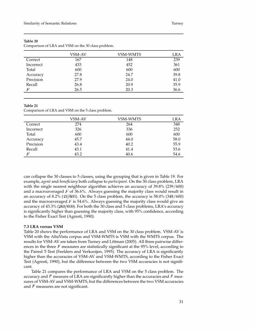
Similarity of Semantic Relations Turney
Table 20Comparison of LRA and VSM on the 30 class problem.
VSM-AV VSM-WMTS LRACorrect 167 148 239Incorrect 433 452 361Total 600 600 600Accuracy 27.8 24.7 39.8Precision 27.9 24.0 41.0Recall 26.8 20.9 35.9� 26.5 20.3 36.6
Table 21Comparison of LRA and VSM on the 5 class problem.
VSM-AV VSM-WMTS LRACorrect 274 264 348Incorrect 326 336 252Total 600 600 600Accuracy 45.7 44.0 58.0Precision 43.4 40.2 55.9Recall 43.1 41.4 53.6� 43.2 40.6 54.6
can collapse the 30 classes to 5 classes, using the grouping that is given in Table 19. Forexample, agent and beneficiary both collapse to participant. On the 30 class problem, LRAwith the single nearest neighbour algorithm achieves an accuracy of 39.8% (239/600)and a macroaveraged � of 36.6%. Always guessing the majority class would result inan accuracy of 8.2% (
������). On the 5 class problem, the accuracy is 58.0% (348/600)
and the macroaveraged � is 54.6%. Always guessing the majority class would give anaccuracy of 43.3% (
�������). For both the 30 class and 5 class problems, LRA’s accuracy
is significantly higher than guessing the majority class, with 95% confidence, accordingto the Fisher Exact Test (Agresti, 1990).
7.3 LRA versus VSMTable 20 shows the performance of LRA and VSM on the 30 class problem. VSM-AV isVSM with the AltaVista corpus and VSM-WMTS is VSM with the WMTS corpus. Theresults for VSM-AV are taken from Turney and Littman (2005). All three pairwise differ-ences in the three � measures are statistically significant at the 95% level, according tothe Paired T-Test (Feelders and Verkooijen, 1995). The accuracy of LRA is significantlyhigher than the accuracies of VSM-AV and VSM-WMTS, according to the Fisher ExactTest (Agresti, 1990), but the difference between the two VSM accuracies is not signifi-cant.
Table 21 compares the performance of LRA and VSM on the 5 class problem. Theaccuracy and � measure of LRA are significantly higher than the accuracies and � mea-sures of VSM-AV and VSM-WMTS, but the differences between the two VSM accuraciesand � measures are not significant.
31
Computational Linguistics Volume 1, Number 1
8. Discussion
The experimental results in Sections 6 and 7 demonstrate that LRA performs signif-icantly better than the VSM, but it is also clear that there is room for improvement.The accuracy might not yet be adequate for practical applications, although past workhas shown that it is possible to adjust the tradeoff of precision versus recall (Turney andLittman, 2005). For some of the applications, such as information extraction, LRA mightbe suitable if it is adjusted for high precision, at the expense of low recall.
Another limitation is speed; it took almost nine days for LRA to answer 374 analogyquestions. However, with progress in computer hardware, speed will gradually becomeless of a concern. Also, the software has not been optimized for speed; there are severalplaces where the efficiency could be increased and many operations are parallelizable.It may also be possible to precompute much of the information for LRA, although thiswould require substantial changes to the algorithm.
The difference in performance between VSM-AV and VSM-WMTS shows that VSMis sensitive to the size of the corpus. Although LRA is able to surpass VSM-AV when theWMTS corpus is only about one tenth the size of the AV corpus, it seems likely that LRAwould perform better with a larger corpus. The WMTS corpus requires one terabyte ofhard disk space, but progress in hardware will likely make ten or even one hundredterabytes affordable in the relatively near future.
For noun-modifier classification, more labeled data should yield performance im-provements. With 600 noun-modifier pairs and 30 classes, the average class has only20 examples. We expect that the accuracy would improve substantially with five or tentimes more examples. Unfortunately, it is time consuming and expensive to acquirehand-labeled data.
Another issue with noun-modifier classification is the choice of classification schemefor the semantic relations. The 30 classes of Nastase and Szpakowicz (2003) might notbe the best scheme. Other researchers have proposed different schemes (Vanderwende,1994; Barker and Szpakowicz, 1998; Rosario and Hearst, 2001; Rosario, Hearst, and Fill-more, 2002). It seems likely that some schemes are easier for machine learning thanothers. For some applications, 30 classes may not be necessary; the 5 class scheme maybe sufficient.
LRA, like VSM, is a corpus-based approach to measuring relational similarity. Pastwork suggests that a hybrid approach, combining multiple modules, some corpus-based, some lexicon-based, will surpass any purebred approach (Turney et al., 2003).In future work, it would be natural to combine the corpus-based approach of LRA withthe lexicon-based approach of Veale (2004), perhaps using the combination method ofTurney et al. (2003).
The Singular Value Decomposition is only one of many methods for handling sparse,noisy data. We have also experimented with Nonnegative Matrix Factorization (NMF)(Lee and Seung, 1999), Probabilistic Latent Semantic Analysis (PLSA) (Hofmann, 1999),Kernel Principal Components Analysis (KPCA) (Scholkopf, Smola, and Muller, 1997),and Iterative Scaling (IS) (Ando, 2000). We had some interesting results with smallmatrices (around 2,000 rows by 1,000 columns), but none of these methods seemed sub-stantially better than SVD and none of them scaled up to the matrix sizes we are usinghere (e.g., 17,232 rows and 8,000 columns; see Section 6.1).
In step 4 of LRA, we simply select the top ��� � ������� most frequent patternsand discard the remaining patterns. Perhaps a more sophisticated selection algorithmwould improve the performance of LRA. We have tried a variety of ways of selectingpatterns, but it seems that the method of selection has little impact on performance. Wehypothesize that the distributed vector representation is not sensitive to the selection
32
Similarity of Semantic Relations Turney
method, but it is possible that future work will find a method that yields significantimprovement in performance.
9. Conclusion
This paper has introduced a new method for calculating relational similarity, LatentRelational Analysis. The experiments demonstrate that LRA performs better than theVSM approach, when evaluated with SAT word analogy questions and with the task ofclassifying noun-modifier expressions. The VSM approach represents the relation be-tween a pair of words with a vector, in which the elements are based on the frequenciesof 64 hand-built patterns in a large corpus. LRA extends this approach in three ways:(1) the patterns are generated dynamically from the corpus, (2) SVD is used to smooththe data, and (3) a thesaurus is used to explore variations of the word pairs. With theWMTS corpus (about � � �� �� English words), LRA achieves an � of 56.5%, whereas the� of VSM is 40.3%.
We have presented several examples of the many potential applications for mea-sures of relational similarity. Just as attributional similarity measures have proven tohave many practical uses, we expect that relational similarity measures will soon be-come widely used. Gentner et al. (2001) argue that relational similarity is essentialto understanding novel metaphors (as opposed to conventional metaphors). Many re-searchers have argued that metaphor is the heart of human thinking (Lakoff and John-son, 1980; Hofstadter and the Fluid Analogies Research Group, 1995; Gentner et al.,2001; French, 2002). We believe that relational similarity plays a fundamental role in themind and therefore relational similarity measures could be crucial for artificial intelli-gence.
In future work, we plan to investigate some potential applications for LRA. It is pos-sible that the error rate of LRA is still too high for practical applications, but the fact thatLRA matches average human performance on SAT analogy questions is encouraging.
33

Computational Linguistics Volume 1, Number 1
Acknowledgments
Thanks to Michael Littman for sharing the 374
SAT analogy questions and for inspiring me to
tackle them. Thanks to Vivi Nastase and Stan
Szpakowicz for sharing their 600 classified noun-
modifier phrases. Thanks to Egidio Terra, Char-
lie Clarke, and the School of Computer Science
of the University of Waterloo, for giving us a
copy of the Waterloo MultiText System and their
Terabyte Corpus. Thanks to Dekang Lin for mak-
ing his Dependency-Based Word Similarity lex-
icon available online. Thanks to Doug Rohde
for SVDLIBC and Michael Berry for SVDPACK.
Thanks to Ted Pedersen for making his Word-
Net::Similarity package available. Thanks to Joel
Martin for comments on the paper. Thanks to
the anonymous reviewers of Computational Lin-
guistics for their very helpful comments and sug-
gestions.
References
Agresti, Alan. 1990. Categorical Data Anal-ysis. Wiley.
Ando, Rie Kubota. 2000. Latent seman-tic space: Iterative scaling improvesprecision of inter-document similaritymeasurement. In Proceedings of the23rd Annual ACM SIGIR Conference onResearch and Development in InformationRetrieval (SIGIR-2000), pages 216–223.
Baeza-Yates, Ricardo A. and Berthier A.Ribeiro-Neto. 1999. Modern Informa-tion Retrieval. ACM Press.
Banerjee, Satanjeev and Ted Pedersen.2003. Extended gloss overlaps as ameasure of semantic relatedness. InProceedings of the Eighteenth Interna-tional Joint Conference on Artificial Intel-ligence (IJCAI-03), pages 805–810, Aca-pulco, Mexico.
Barker, Ken and Stan Szpakowicz. 1998.Semi-automatic recognition of nounmodifier relationships. In ChristianBoitet and Pete Whitelock, editors,Proceedings of the Thirty-Sixth AnnualMeeting of the Association for Compu-
tational Linguistics and Seventeenth In-ternational Conference on ComputationalLinguistics (COLING-ACL’98), pages96–102, San Francisco, California.Morgan Kaufmann Publishers.
Berland, Matthew and Eugene Charniak.1999. Finding parts in very large cor-pora. In Proceedings of the 37th AnnualMeeting of the Association for Computa-tional Linguistics (ACL ’99), pages 57–64, New Brunswick, NJ.
Berry, Michael W. 1992. Large scale singu-lar value computations. InternationalJournal of Supercomputer Applications,6(1):13–49.
Budanitsky, Alexander and Graeme Hirst.2001. Semantic distance in wordnet:An experimental, application-orientedevaluation of five measures. In Pro-ceedings of the Workshop on WordNet andOther Lexical Resources, Second Meet-ing of the North American Chapter of theAssociation for Computational Linguis-tics (NAACL-2001), pages 29–24, Pitts-burgh, PA.
Chiarello, Christine, Curt Burgess, LorieRichards, and Alma Pollock. 1990. Se-mantic and associative priming in thecerebral hemispheres: Some words do,some words don’t ... sometimes, someplaces. Brain and Language, 38:75–104.
Claman, Cathy. 2000. 10 Real SATs. Col-lege Entrance Examination Board.
Clarke, Charles L.A., Gordon V. Cormack,and Christopher R. Palmer. 1998. Anoverview of multitext. ACM SIGIR Fo-rum, 32(2):14–15.
Daganzo, Carlos F. 1994. The cell trans-mission model: A dynamic represen-tation of highway traffic consistentwith the hydrodynamic theory. Trans-portation Research Part B: Methodologi-cal, 28(4):269–287.
Deerwester, Scott C., Susan T. Dumais,Thomas K. Landauer, George W. Fur-nas, and Richard A. Harshman. 1990.
34
Similarity of Semantic Relations Turney
Indexing by latent semantic analysis.Journal of the American Society for Infor-mation Science (JASIS), 41(6):391–407.
Dolan, William B. 1995. Metaphoras an emergent property of machine-readable dictionaries. In Proceedings ofthe AAAI 1995 Spring Symposium Series:Representation and Acquisition of Lexi-cal Knowledge: Polysemy, Ambiguity andGenerativity, pages 27–32.
Dumais, Susan T. 1990. Enhancingperformance in latent semantic index-ing (LSI) retrieval. Technical Re-port TM-ARH-017527, Bellcore, Mor-ristown, NJ.
Dumais, Susan T. 1993. Latent semanticindexing (LSI) and TREC-2. In D.K.Harman, editor, Proceedings of the Sec-ond Text REtrieval Conference (TREC-2), pages 105–115. National Institute ofStandards and Technology.
Falkenhainer, Brian. 1990. Analogical in-terpretation in context. In Proceedingsof the Twelfth Annual Conference of theCognitive Science Society, pages 69–76.Lawrence Erlbaum Associates.
Falkenhainer, Brian, Kenneth D. Forbus,and Dedre Gentner. 1989. Thestructure-mapping engine: Algorithmand examples. Artificial Intelligence,41(1):1–63.
Federici, Stefano, Simonetta Montemagni,and Vito Pirrelli. 1997. Inferring se-mantic similarity from distributionalevidence: An analogy-based approachto word sense disambiguation. InProceedings of the ACL/EACL Work-shop on Automatic Information Extrac-tion and Building of Lexical Semantic Re-sources for NLP Applications, pages 90–97, Madrid, Spain.
Feelders, Ad and William Verkooijen.1995. Which method learns the mostfrom data? Methodological issues inthe analysis of comparative studies. InFifth International Workshop on Artificial
Intelligence and Statistics, pages 219–225, Ft. Lauderdale, Florida.
Fellbaum, Christiane, editor. 1998. Word-Net: An Electronic Lexical Database.MIT Press.
French, Robert M. 2002. The compu-tational modeling of analogy-making.Trends in Cognitive Sciences, 6(5):200–205.
Gentner, Dedre. 1983. Structure-mapping:A theoretical framework for analogy.Cognitive Science, 7(2):155–170.
Gentner, Dedre, Brian Bowdle, PhillipWolff, and Consuelo Boronat. 2001.Metaphor is like analogy. In DedreGentner, Keith J. Holyoak, and Boi-cho N. Kokinov, editors, The AnalogicalMind: Perspectives from Cognitive Sci-ence, pages 199–253, Cambridge, MA.MIT Press.
Gildea, Daniel and Daniel Jurafsky. 2002.Automatic labeling of semantic roles.Computational Linguistics, 28(3):245–288.
Girju, Roxana, Adriana Badulescu, andDan I. Moldovan. 2003. Learn-ing semantic constraints for the au-tomatic discovery of part-whole rela-tions. In Proceedings of the Human Lan-guage Technology Conference of the NorthAmerican Chapter of the Association forComputational Linguistics (HLT-NAACL2003), pages 80–87.
Goldenberg, David. 2005. The em-peror’s new clothes: Undressingthe new and unimproved sat. GelfMagazine, March. http://www.gelf-magazine.com/mt/archives/the emp-erors new clothes.html.
Golub, Gene H. and Charles F. Van Loan.1996. Matrix Computations. JohnsHopkins University Press, Baltimore,MD, third edition.
Harman, Donna. 1986. An experimen-tal study of factors important in doc-ument ranking. In Proceedings of the
35

Computational Linguistics Volume 1, Number 1
Ninth Annual International ACM SI-GIR Conference on Research and De-velopment in Information Retrieval (SI-GIR’86), pages 186–193, Pisa, Italy.
Hearst, Marti A. 1992. Automatic ac-quisition of hyponyms from large textcorpora. In Proceedings of the Four-teenth International Conference on Com-putational Linguistics, pages 539–545,Nantes, France.
Hirst, Graeme and David St-Onge. 1998.Lexical chains as representations ofcontext for the detection and correc-tion of malapropisms. In ChristianeFellbaum, editor, WordNet: An Elec-tronic Lexical Database, pages 305–332.MIT Press.
Hofmann, Thomas. 1999. ProbabilisticLatent Semantic Indexing. In Proceed-ings of the 22nd Annual ACM Conferenceon Research and Development in Informa-tion Retrieval (SIGIR ’99), pages 50–57,Berkeley, California, August.
Hofstadter, Douglas and the Fluid Analo-gies Research Group. 1995. Fluid Con-cepts and Creative Analogies: ComputerModels of the Fundamental Mechanismsof Thought. Basic Books, New York,NY.
Jarmasz, Mario and Stan Szpakowicz.2003. Roget’s thesaurus and semanticsimilarity. In Proceedings of the Interna-tional Conference on Recent Advances inNatural Language Processing (RANLP-03), pages 212–219, Borovets, Bulgaria.
Jiang, Jay J. and David W. Conrath. 1997.Semantic similarity based on corpusstatistics and lexical taxonomy. In Pro-ceedings of the International Conferenceon Research in Computational Linguistics(ROCLING X), pages 19–33, Tapei, Tai-wan.
Kurtz, Stanley. 2002. Testing debate.National Review Magazine, August.http://www.nationalreview.com/kur-tz/kurtz082102.asp.
Lakoff, George and Mark Johnson. 1980.Metaphors We Live By. University ofChicago Press, Chicago, IL.
Landauer, Thomas K. and Susan T. Du-mais. 1997. A solution to Plato’s prob-lem: The latent semantic analysis the-ory of the acquisition, induction, andrepresentation of knowledge. Psycho-logical Review, 104(2):211–240.
Lapata, Mirella and Frank Keller. 2004.The web as a baseline: Evaluating theperformance of unsupervised web-based models for a range of NLPtasks. In Proceedings of the Human Lan-guage Technology Conference of the NorthAmerican Chapter of the Association forComputational Linguistics (HLT-NAACL2004), pages 121–128.
Lauer, Mark. 1995. Designing StatisticalLanguage Learners: Experiments on Com-pound Nouns. Ph.D. thesis, MacquarieUniversity.
Leacock, Claudia and Martin Chodorow.1998. Combining local context andWordNet similarity for word senseidentification. In Christiane Fellbaum,editor, WordNet: An Electronic LexicalDatabase, pages 265–283. MIT Press.
Lee, Daniel D. and H. Sebastian Seung.1999. Learning the parts of objects bynonnegative matrix factorization. Na-ture, 401:788–791.
Lesk, Michael E. 1969. Word-word associ-ations in document retrieval systems.American Documentation, 20(1):27–38.
Lesk, Michael E. 1986. Automatic sensedisambiguation using machine read-able dictionaries: How to tell a pinecone from a ice cream cone. In Proceed-ings of ACM SIGDOC ’86, pages 24–26.
Lewis, David D. 1991. Evaluating text cat-egorization. In Proceedings of the Speechand Natural Language Workshop, pages312–318, Asilomar, CA. Morgan Kauf-mann.
36
Similarity of Semantic Relations Turney
Lin, Dekang. 1998a. Automatic retrievaland clustering of similar words. InProceedings of the 36th Annual Meet-ing of the Association for ComputationalLinguistics and the 17th InternationalConference on Computational Linguis-tics (COLING-ACL ’98), pages 768–774,Montreal, Canada.
Lin, Dekang. 1998b. An information-theoretic definition of similarity. InProceedings of the 15th International Con-ference on Machine Learning (ICML ’98),pages 296–304. Morgan Kaufmann,San Francisco, CA.
Marx, Zvika, Ido Dagan, Joachim Buh-mann, and Eli Shamir. 2002. Cou-pled clustering: A method for detect-ing structural correspondence. Jour-nal of Machine Learning Research, 3:747–780.
Medin, Douglas L., Robert L. Goldstone,and Dedre Gentner. 1990. Similar-ity involving attributes and relations:Judgments of similarity and differenceare not inverses. Psychological Science,1(1):64–69.
Moldovan, Dan, Adriana Badulescu,Marta Tatu, Daniel Antohe, andRoxana Girju. 2004. Models forthe semantic classification of nounphrases. In Proceedings of the Com-putational Lexical Semantics Workshopat HLT-NAACL 2004, pages 60–67,Boston, MA.
Morris, Jane and Graeme Hirst. 1991. Lex-ical cohesion computed by thesauralrelations as an indicator of the struc-ture of text. Computational Linguistics,17(1):21–48.
Nastase, Vivi and Stan Szpakowicz. 2003.Exploring noun-modifier semantic re-lations. In Fifth International Workshopon Computational Semantics (IWCS-5),pages 285–301, Tilburg, The Nether-lands.
Pantel, Patrick and Dekang Lin. 2002. Dis-covering word senses from text. In
Proceedings of ACM SIGKDD Confer-ence on Knowledge Discovery and DataMining, pages 613–619.
Rada, Roy, Hafedh Mili, Ellen Bicknell,and Maria Blettner. 1989. Develop-ment and application of a metric on se-mantic nets. IEEE Transactions on Sys-tems, Man, and Cybernetics, 19(1):17–30.
Rehder, Bob, M.E. Schreiner, Michael B.W.Wolfe, Darrell Laham, Thomas K. Lan-dauer, and Walter Kintsch. 1998. Us-ing latent semantic analysis to assessknowledge: Some technical considera-tions. Discourse Processes, 25:337–354.
Reitman, Walter R. 1965. Cognition andThought: An Information Processing Ap-proach. John Wiley and Sons, NewYork, NY.
Resnik, Philip. 1995. Using informa-tion content to evaluate semantic sim-ilarity in a taxonomy. In Proceedingsof the 14th International Joint Confer-ence on Artificial Intelligence (IJCAI-95),pages 448–453, San Mateo, CA. Mor-gan Kaufmann.
Riloff, Ellen and Rosie Jones. 1999.Learning dictionaries for informationextraction by multi-level bootstrap-ping. In Proceedings of the Sixteenth Na-tional Conference on Artificial Intelligence(AAAI-99), pages 474–479.
Rosario, Barbara and Marti Hearst.2001. Classifying the semantic re-lations in noun-compounds via adomain-specific lexical hierarchy. InProceedings of the 2001 Conference onEmpirical Methods in Natural LanguageProcessing (EMNLP-01), pages 82–90.
Rosario, Barbara, Marti Hearst, andCharles Fillmore. 2002. The de-scent of hierarchy, and selection in re-lational semantics. In Proceedings of the40th Annual Meeting of the Associationfor Computational Linguistics (ACL ’02),pages 417–424, Philadelphia, PA.
37

Computational Linguistics Volume 1, Number 1
Ruge, Gerda. 1992. Experiments onlinguistically-based term associations.Information Processing and Management,28(3):317–332.
Salton, Gerard. 1989. Automatic TextProcessing: The Transformation, Analy-sis, and Retrieval of Information by Com-puter. Addison-Wesley, Reading, MA.
Salton, Gerard and Chris Buckley. 1988.Term-weighting approaches in auto-matic text retrieval. Information Pro-cessing and Management, 24(5):513–523.
Salton, Gerard and Michael J. McGill.1983. Introduction to Modern Infor-mation Retrieval. McGraw-Hill, NewYork, NY.
Scholkopf, Bernhard, Alexander J. Smola,and Klaus-Robert Muller. 1997. Ker-nel principal component analysis. InProceedings of the International Con-ference on Artificial Neural Networks(ICANN-1997), pages 583–588, Berlin.
Terra, Egidio and Charles L.A. Clarke.2003. Frequency estimates for statis-tical word similarity measures. In Pro-ceedings of the Human Language Technol-ogy and North American Chapter of Asso-ciation of Computational Linguistics Con-ference 2003 (HLT/NAACL 2003), pages244–251.
Turney, Peter D. 2001. Mining the Webfor synonyms: PMI-IR versus LSA onTOEFL. In Proceedings of the TwelfthEuropean Conference on Machine Learn-ing, pages 491–502, Berlin. Springer.
Turney, Peter D. 2002. Thumbs upor thumbs down? Semantic orienta-tion applied to unsupervised classifi-cation of reviews. In Proceedings of the40th Annual Meeting of the Associationfor Computational Linguistics (ACL’02),pages 417–424.
Turney, Peter D. 2005. Measuring seman-tic similarity by latent relational anal-ysis. In Proceedings of the Nineteenth
International Joint Conference on Artifi-cial Intelligence (IJCAI-05), pages 1136–1141, Edinburgh, Scotland.
Turney, Peter D. and Michael L. Littman.2005. Corpus-based learning of analo-gies and semantic relations. MachineLearning, 60(1–3):251–278.
Turney, Peter D., Michael L. Littman, Jef-frey Bigham, and Victor Shnayder.2003. Combining independent mod-ules to solve multiple-choice synonymand analogy problems. In Proceed-ings of the International Conference onRecent Advances in Natural LanguageProcessing (RANLP-03), pages 482–489,Borovets, Bulgaria.
Vanderwende, Lucy. 1994. Algorithmfor automatic interpretation of nounsequences. In Proceedings of the Fif-teenth International Conference on Com-putational Linguistics, pages 782–788,Kyoto, Japan.
Veale, Tony. 2003. The analogical the-saurus. In Proceedings of the 15th In-novative Applications of Artificial Intel-ligence Conference (IAAI 2003), pages137–142, Acapulco, Mexico.
Veale, Tony. 2004. WordNet sits the SAT:A knowledge-based approach to lexi-cal analogy. In Proceedings of the 16thEuropean Conference on Artificial Intelli-gence (ECAI 2004), pages 606–612, Va-lencia, Spain.
Yangarber, Roman. 2003. Counter-training in discovery of semantic pat-terns. In Proceedings of the 41st AnnualMeeting of the Association for Compu-tational Linguistics (ACL-2003), pages343–350, Sapporo, Japan.
Yarowsky, David. 1993. One sense percollocation. In Proceedings of the ARPAHuman Language Technology Workshop,pages 266–271, Princeton, NJ.
Zelenko, Dmitry, Chinatsu Aone, and An-thony Richardella. 2003. Kernel meth-ods for relation extraction. Journal
38

Similarity of Semantic Relations Turney
of Machine Learning Research, 3:1083–1106.
39