SimClimat documentation

Camille Risi

November 2019

A web version of this documentation is on http://www.lmd.jussieu.fr/~crlmd/simclimat/documentation_

2019

The SimClimat software is an educational software for climate simulations ([Risi, 2015]). Through a user-friendlyinterface, it allows to run climate simulations at different time scales. The results pertaining to global surfacetemperature, sea level, ice sheet expansion and atmospheric composition are displayed as curves and drawings. Theuser can test the influence of various parameters influencing the climate, such as astronomical parameters or thecomposition of the atmosphere, and can plug or unplug some climate feedbacks.

SimClimat is composed of a graphical interface coupled to a physical climate model. This documentation firstdescribes the graphical interface (section 1) and then the physical model (section 2). This documentation alsopresents how to implement the experimental method with SimClimat in a classroom (section 3). The physicalcontent and results of SimClimat are compared to the "true" climate models used in the IPCC reports (section 4).

Table des matières

1 Graphical interface 2

1.1 Supported platforms . . . . . . . . . . . . . . . . . . . . . . . . . . . . . . . . . . . . . . . . . . . . . 21.2 Inputs . . . . . . . . . . . . . . . . . . . . . . . . . . . . . . . . . . . . . . . . . . . . . . . . . . . . . 2

1.2.1 Initial state . . . . . . . . . . . . . . . . . . . . . . . . . . . . . . . . . . . . . . . . . . . . . . 21.2.2 Duration . . . . . . . . . . . . . . . . . . . . . . . . . . . . . . . . . . . . . . . . . . . . . . . 31.2.3 Color and name . . . . . . . . . . . . . . . . . . . . . . . . . . . . . . . . . . . . . . . . . . . 31.2.4 Parameters . . . . . . . . . . . . . . . . . . . . . . . . . . . . . . . . . . . . . . . . . . . . . . 4

1.3 Outputs . . . . . . . . . . . . . . . . . . . . . . . . . . . . . . . . . . . . . . . . . . . . . . . . . . . . 41.3.1 Curves . . . . . . . . . . . . . . . . . . . . . . . . . . . . . . . . . . . . . . . . . . . . . . . . . 61.3.2 Drawings . . . . . . . . . . . . . . . . . . . . . . . . . . . . . . . . . . . . . . . . . . . . . . . 61.3.3 Export in .csv format . . . . . . . . . . . . . . . . . . . . . . . . . . . . . . . . . . . . . . . . 6

1.4 Small user’s guide . . . . . . . . . . . . . . . . . . . . . . . . . . . . . . . . . . . . . . . . . . . . . . 6

2 The physical model of SimClimat 7

2.1 Observational constraints on the model . . . . . . . . . . . . . . . . . . . . . . . . . . . . . . . . . . 72.2 Temporal integration . . . . . . . . . . . . . . . . . . . . . . . . . . . . . . . . . . . . . . . . . . . . . 72.3 Global radiative equilibrium model . . . . . . . . . . . . . . . . . . . . . . . . . . . . . . . . . . . . . 8

2.3.1 Absorbed solar flux . . . . . . . . . . . . . . . . . . . . . . . . . . . . . . . . . . . . . . . . . . 82.3.2 Infrared radiation emitted by the Earth . . . . . . . . . . . . . . . . . . . . . . . . . . . . . . 82.3.3 Equilibrium temperature . . . . . . . . . . . . . . . . . . . . . . . . . . . . . . . . . . . . . . 9

2.4 Coupling the radiative equilibrium model with the other components . . . . . . . . . . . . . . . . . 92.4.1 Greenhouse effect . . . . . . . . . . . . . . . . . . . . . . . . . . . . . . . . . . . . . . . . . . . 92.4.2 Albedo . . . . . . . . . . . . . . . . . . . . . . . . . . . . . . . . . . . . . . . . . . . . . . . . . 92.4.3 Sea level . . . . . . . . . . . . . . . . . . . . . . . . . . . . . . . . . . . . . . . . . . . . . . . . 11

3 Implementing the experimental method with SimClimat 11

3.1 Why do we need numerical modeling? . . . . . . . . . . . . . . . . . . . . . . . . . . . . . . . . . . . 113.2 Implementing the experimental method with SimClimat: examples . . . . . . . . . . . . . . . . . . . 11

3.2.1 Role of human activities in the observed recent global warming . . . . . . . . . . . . . . . . 113.2.2 Climate feedbacks at play in the recent global warming . . . . . . . . . . . . . . . . . . . . . 113.2.3 Mechanisms at play in glacial-interglacial variations . . . . . . . . . . . . . . . . . . . . . . . 13

1

4 Comparing SimClimat to climate models used in IPCC reports 15

4.1 What kind of models are used for climate projections in IPCC reports? . . . . . . . . . . . . . . . . 154.2 How does a climate model work? . . . . . . . . . . . . . . . . . . . . . . . . . . . . . . . . . . . . . . 164.3 Comparing the physical content . . . . . . . . . . . . . . . . . . . . . . . . . . . . . . . . . . . . . . . 164.4 Comparing climate projections by SimClimat and climate models . . . . . . . . . . . . . . . . . . . . 164.5 Climate feedbacks involved in global warming . . . . . . . . . . . . . . . . . . . . . . . . . . . . . . . 164.6 Role of human activities in current global warming . . . . . . . . . . . . . . . . . . . . . . . . . . . . 20

5 Appendix: equation details for the physical model 20

5.1 Evolution of global temperature . . . . . . . . . . . . . . . . . . . . . . . . . . . . . . . . . . . . . . . 205.2 The greenhouse effect . . . . . . . . . . . . . . . . . . . . . . . . . . . . . . . . . . . . . . . . . . . . 20

5.2.1 The two components of the greenhouse effect . . . . . . . . . . . . . . . . . . . . . . . . . . . 205.2.2 The greenhouse effect related to CO2 as a function of CO2 concentration . . . . . . . . . . . 225.2.3 The greenhouse effect related to water vapor as a function of the water vapor concentration . 225.2.4 The water vapor concentration as a function of temperature . . . . . . . . . . . . . . . . . . . 22

5.3 The carbon cycle . . . . . . . . . . . . . . . . . . . . . . . . . . . . . . . . . . . . . . . . . . . . . . . 225.3.1 Biological storage and continental alteration . . . . . . . . . . . . . . . . . . . . . . . . . . . . 235.3.2 CO2 solubility in the ocean . . . . . . . . . . . . . . . . . . . . . . . . . . . . . . . . . . . . . 235.3.3 Absorption of part of CO2 emissions by the ocean and the vegetation . . . . . . . . . . . . . 23

5.4 Albedo and ice sheets . . . . . . . . . . . . . . . . . . . . . . . . . . . . . . . . . . . . . . . . . . . . 235.4.1 Albedo as a function of ice sheet extension . . . . . . . . . . . . . . . . . . . . . . . . . . . . 235.4.2 Ice sheet extent as a function of temperature and of summer insolation at 65°N . . . . . . . . 235.4.3 Summer insolation at 65°N . . . . . . . . . . . . . . . . . . . . . . . . . . . . . . . . . . . . . 24

5.5 Sea level . . . . . . . . . . . . . . . . . . . . . . . . . . . . . . . . . . . . . . . . . . . . . . . . . . . . 24

1 Graphical interface

1.1 Supported platforms

SimClimat works on personal computers with Windows and on smart-phones with Android or Mac-OS. Theinterface automatically adapts to the screen.

1.2 Inputs

A simulation is defined by :

1. An initial state : initial values for temperature, CO2 concentration, sea level and ice sheet extent ;

2. A duration : number of years of simulation ;

3. A simulation name and its color ;

4. Parameters determining the behavior of the model during the simulation.

1.2.1 Initial state

In the interface, the initial state can be chosen in the page following the home page (figures 1,2). The possibleinitial states are :

1. "Today’s world" : The temperature is 15.3°C, the CO2 concentration is 405 ppm,CO2 emissions are 8 GtC/year,the sea level is 0 m.

2. "The pre-industrial world" : The climatic variables are those of the pre-industrial era : the temperature is14.4 ° C, the CO2 concentration is 280 ppm, the sea level of -0.2m , CO2 emissions are null.

3. "The final state of the previous simulation" : This allows to continue the previous simulation.

4. "The final state of a saved simulation" : If a final state of a simulation has already been saved, it is possibleto start a simulation with this state. This allows to continue an earlier simulation.

2

Figure 1 – Screenshot of the home page of SimClimat with Windows.

Figure 2 – Screenshot of the page where the intial state and the duration can be chosen, with Windows.

1.2.2 Duration

The duration can be chosen in the same page as the initial state (figures 1,2). It can be between 100 years and10 million years. The deadline depends on the processes that we wants to study. For example, to study current globalwarming, durations of 100 to 500 years are recommended. To study the glacial-interglacial variations in which theice sheets are at play, durations of tens to hundreds of thousands of years are recommended. To study continentalweathering, durations of several million years are recommended.

1.2.3 Color and name

In the interface, the color and name can be chosen in the second page (figure 3). They can still be modified oncethe simulation is launched using the “curve” icon (figure 5).

3

Figure 3 – Screenshot of the page where the simulation name and color can be chosen, withWindows.

1.2.4 Parameters

We can tune 3 kinds of parameters :

1. astronomical parameters (example in section 3.2.3) :– Earth-Sun Distance– Solar power– Eccentricity– Obliquity– Precession

2. CO2 concentration or emissions : we can choose between 2 types of simulations :– Set the CO2 concentration : The concentration is constant throughout the simulation, whatever CO2 fluxes,

and is chosen by the user (example in section 3.2.1)..– Set emissions : The concentration is calculated interactively by the model, according to the sources or sinks

chosen by the user. Sources or sinks that the user can tune are :– Anthropogenic emissions– Volcanism and oceanic ridge activity– Continental alteration– Biological storage

3. climate feedbacks : Four types of climate feedback are taken into account and can be optionally tuned orunplugged by the user :– Albedo– Ocean– Vegetation– Water vapor

For each parameter, we can show a small explanatory text and/or a schematic (example : figure 4).Once the simulation is launched, we can check the value of all parameters using the “eye” icon, or modify

parameters with the “key” icon (figure 6).

1.3 Outputs

The model results are displayed in the interface through curves and drawings or can be exported in differentformats.

4

Figure 4 – Screenshot of the page where parameters associated with the carbon cycle can be chosen, on Windows.

Figure 5 – Screenshot of the page where results are displayed, on Windows.

5

Figure 6 – Screenshot of the page where results are displayed, when the “Edit simulations” icon is activated, onWindows.

1.3.1 Curves

Curves display :

1. The global, annual-mean temperature at the Earth’s surface, in °C

2. The CO2 concentration, in ppm

3. CO2 emissions, in Gt of Carbone per year (GtC/year)

4. The sea level

5. The latitude of ice sheers, in ° of latitude

6. The global-mean planetary albedo, without unity.

The curves display time in x-axis, in year after JC, and the displayed variable in y-axis.When superimposing several simulations, the curves are displayed in different colors. The color code connecting

the color to the simulation names is indicated in the key.

1.3.2 Drawings

Two types of drawings are displayed :– an Earth, on which we can see the ice-sheet extent ; beware that this extent is very approximate.– a tropical island, where you can see the sea level.

1.3.3 Export in .csv format

Simulation results may be downloaded as .csv numerical format, which can then be opened as an Excell scheet.To do so, click on the «download» icon near the top-right corner (figure 5).

1.4 Small user’s guide

– Launch a first simulation : Click on ”New simulation”, then chose the input parameters (section 1.2). Launchthe simulation by clicking on the small orange arrow..

– Add another simulation : In the display page, click on the ”+” icon. Chose the new input parameters.– Modifiy a simulation name and/or color : In the display page, click on the ”Curves” icon. The simulation list

appears on the left. Click on the ”pencil” icon to edit the name or to select a new color.– Show the input parameters for a simulation : In the display page, click on the ”Curves” icon.. The simulation

list appears on the left. Click on the “eye” to show all parameters.

6

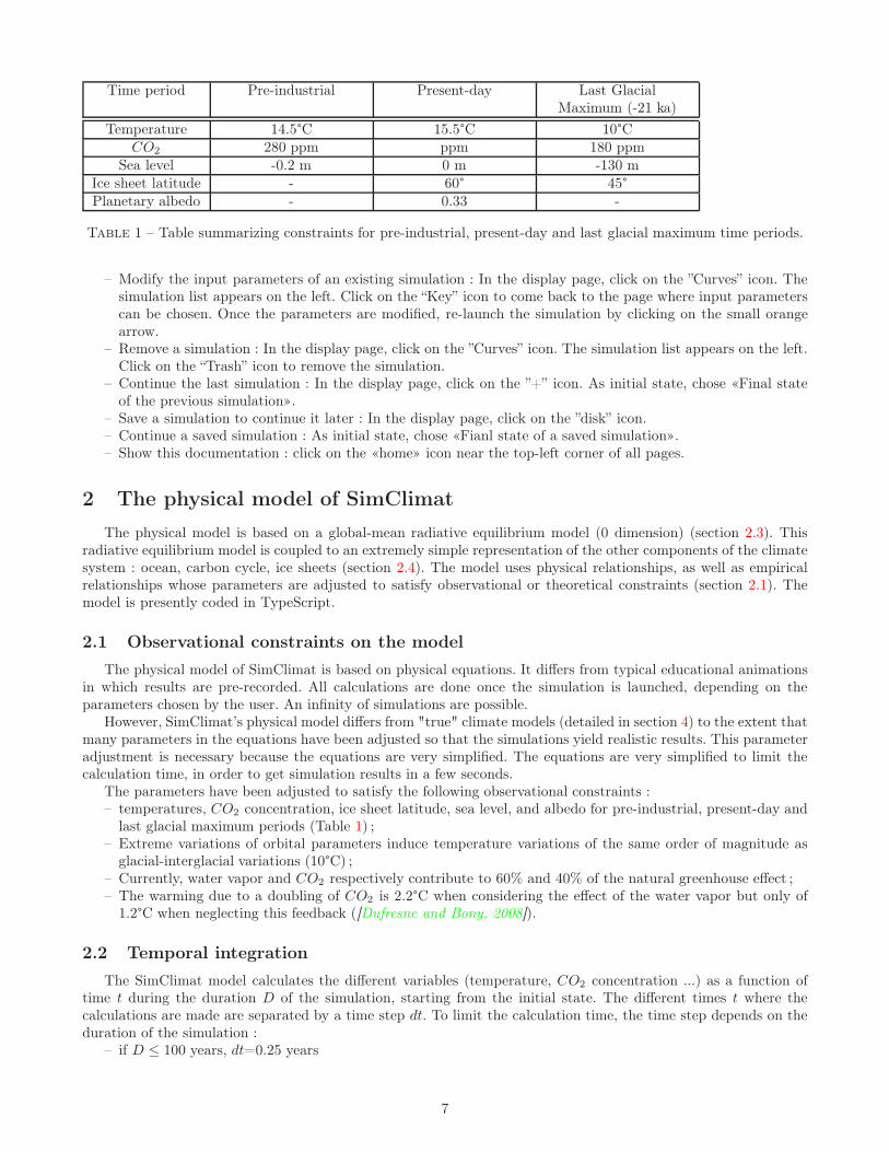
Time period Pre-industrial Present-day Last GlacialMaximum (-21 ka)

Temperature 14.5°C 15.5°C 10°CCO2 280 ppm ppm 180 ppm

Sea level -0.2 m 0 m -130 mIce sheet latitude - 60° 45°Planetary albedo - 0.33 -

Table 1 – Table summarizing constraints for pre-industrial, present-day and last glacial maximum time periods.

– Modify the input parameters of an existing simulation : In the display page, click on the ”Curves” icon. Thesimulation list appears on the left. Click on the “Key” icon to come back to the page where input parameterscan be chosen. Once the parameters are modified, re-launch the simulation by clicking on the small orangearrow.

– Remove a simulation : In the display page, click on the ”Curves” icon. The simulation list appears on the left.Click on the “Trash” icon to remove the simulation.

– Continue the last simulation : In the display page, click on the ”+” icon. As initial state, chose «Final stateof the previous simulation».

– Save a simulation to continue it later : In the display page, click on the ”disk” icon.– Continue a saved simulation : As initial state, chose «Fianl state of a saved simulation».– Show this documentation : click on the «home» icon near the top-left corner of all pages.

2 The physical model of SimClimat

The physical model is based on a global-mean radiative equilibrium model (0 dimension) (section 2.3). Thisradiative equilibrium model is coupled to an extremely simple representation of the other components of the climatesystem : ocean, carbon cycle, ice sheets (section 2.4). The model uses physical relationships, as well as empiricalrelationships whose parameters are adjusted to satisfy observational or theoretical constraints (section 2.1). Themodel is presently coded in TypeScript.

2.1 Observational constraints on the model

The physical model of SimClimat is based on physical equations. It differs from typical educational animationsin which results are pre-recorded. All calculations are done once the simulation is launched, depending on theparameters chosen by the user. An infinity of simulations are possible.

However, SimClimat’s physical model differs from "true" climate models (detailed in section 4) to the extent thatmany parameters in the equations have been adjusted so that the simulations yield realistic results. This parameteradjustment is necessary because the equations are very simplified. The equations are very simplified to limit thecalculation time, in order to get simulation results in a few seconds.

The parameters have been adjusted to satisfy the following observational constraints :– temperatures, CO2 concentration, ice sheet latitude, sea level, and albedo for pre-industrial, present-day and

last glacial maximum periods (Table 1) ;– Extreme variations of orbital parameters induce temperature variations of the same order of magnitude as

glacial-interglacial variations (10°C) ;– Currently, water vapor and CO2 respectively contribute to 60% and 40% of the natural greenhouse effect ;– The warming due to a doubling of CO2 is 2.2°C when considering the effect of the water vapor but only of

1.2°C when neglecting this feedback ([Dufresne and Bony, 2008]).

2.2 Temporal integration

The SimClimat model calculates the different variables (temperature, CO2 concentration ...) as a function oftime t during the duration D of the simulation, starting from the initial state. The different times t where thecalculations are made are separated by a time step dt. To limit the calculation time, the time step depends on theduration of the simulation :

– if D ≤ 100 years, dt=0.25 years

7

reflected

incidentradiation

radiationinfrared

radiation

greenhouse

(1− α) · S0 = (1−G) · σ · T 4

(1−G) · σ · T 4

α · S0

σ · T 4

gases

atmosphere

Earth

S0

Figure 7 – Global radiative equilibrium model.

– if D > 100 years, dt = (D0.7) · 1000.3/300. For example, dt ≃ 210 years for D = 1 million years, and dt ≃ 5283years pour D = 100 million years.

2.3 Global radiative equilibrium model

At radiative equilibrium, the solar flux that is absorbed by the Earth, Fin, equals the infra-red radiation emittedby the Earth, Fout (figure 7) :

Fin = Fout

Fluxes Fin and Fout are expressed in W/m2.

2.3.1 Absorbed solar flux

Fin depends on the planetary albedo :

Fin = (1−A) · Fin

0

A is the Earth albedo, which depends on the ice sheet extent. It is computed as detailed in section 2.4.F

in

0 is the global-mean, annual-mean incoming solar flux at the top of the atmosphere. Since at any time, theSun lights up only a quarter of the Earth, we have F in

0 = S0

4 , where S0 = 1370W/m2 is the solar constant.

2.3.2 Infrared radiation emitted by the Earth

Fout depends on temperature according to Stefan-Boltzmann’s law, and is modulated by the greenhouse effect :

Fout = (1−G) · σ · T4

where :G is the greenhouse effect : it is the fraction of infrared radiation emitted by the Earth that is retained by the

greenhouse effect and fails to escape to space ;σ is Stefan-Boltzmann’s constant.This relationship is illustrated for different CO2 concentration in figure 8.

8

0

50

100

150

200

250

300

350

400

450

500

100 150 200 250 300 350

Temperature (K)

Fin

,

Fout

Fout, CO2 = 62500ppm

Fout, CO2 = 12500ppm

Fout, CO2 = 2500ppm

Fout, CO2 = 100ppm

Fin

Fout, CO2 = 500ppm

Figure 8 – Absorbed solar radiation (Fin) and infra-red radiation emitted by the Earth (Fout), as a function oftemperature. Radiative equilibrium is reached for intersection points between Fin(T ) and Fout(T ) curves.

2.3.3 Equilibrium temperature

We calculate Teq(t) at each time step t, assuming radiative balance :

Teq(t) =

(

(1−A(t)) · Fin

0

(1−G(t)) · σ

)1/4

Graphically, Teq corresponds to the intersection point T between Fin(T ) and Fout(T ) curves (figure 8).The temperature T (t) simulated by SimClimat follows the equilibrium temperature Teq, but with some delay to

represent the effect of the thermal inertia of the oceans (section 5.1).

2.4 Coupling the radiative equilibrium model with the other components

To calculate Teq, we need the albedo A and the greenhouse effect G. It is from these variables that the radiativemodel is coupled to the atmospheric composition, to the carbon cycle and to the ice sheets. All these coupledcomponents are represented in figure 9.

2.4.1 Greenhouse effect

The greenhouse effect G is decomposed into two components : the greenhouse effect associated with CO2 (GserreCO2

)and that associated with water vapor (Gserre

H2O) (section 5.2.1).

– The greenhouse effect associated with the water vapor is calculated according to the water vapor concentrationRH2O (section 5.2.3), which is calculated as a function of temperature (section 5.2.4).

– The greenhouse effect associated with CO2 is calculated as a function of CO2 concentration (section 5.2.2).This concentration is calculated from CO2 sources and sinks (anthropogenic emissions, volcanism, continentalalteration, biological storage, storage by the ocean) (section 5.3). The CO2 solubility in the ocean is a functionof temperature (5.3.2).

2.4.2 Albedo

Albedo A is calculated as a function of ice sheet extent φg (section 5.4.1). This extent is calculated as a functionof temperature and of the insolation at 65°N I (section 5.4.2). This insolation is determined by astronomical andorbital parameters.

9

I

insolationà 65N

F in0

solarconstant

Teq

equilibriumtemperature

Geffet de serre

CO2 effect

GserreCO2water vapor effect

GserreH2O

RH2O

atmospheric water vapor

CO2

oceanic fluxes

CO2

sources and sinks

φeqg

ice sheet extentat equilibrium

CO2

atmosphericCO2 concentration

NSea level

φg

Ice sheet latitudeA

Albedo

T

temperature

Volcanism

VegetationContinental alteration

Solar power

Orbital parmetersEarth-Sun distance

Figure 9 – Diagram illustrating how the different variables are computed in the model. In red : external forcingon the climate system. In blue : state variables.

10

2.4.3 Sea level

Sea levels depend both on temperature, through thermal expansion, and on ice sheet extent, which controls theavailable liquid water (section 5.5).

3 Implementing the experimental method with SimClimat

3.1 Why do we need numerical modeling ?

The study of climate change is a special scientific field, where the classical experimental method is not alwaysapplicable. For example, we observe that for 150 years, the global temperature of the Earth has warmed by about 1°C.In parallel, the atmospheric concentration of CO2, a greenhouse gas emitted by human activities, has increased.Is the temperature rise cause by the increase in CO2 concentration ? Or is it pure coincidence ? To answer thisquestion according to the classical experimental method, one should duplicate our planet, make it go back 150years earlier, and let it evolve until now without emitting any CO2, and then accelerate the time to quickly get theresults. Impossible ! Except through numerical modeling. The goal of numerical modeling is precisely to be able tocreate as many Earth planets as one wants, submit them to the CO2 concentration one wants, go back in time, oraccelerate the time... The experimental method is thus based on numerical experiments.

3.2 Implementing the experimental method with SimClimat : examples

3.2.1 Role of human activities in the observed recent global warming

The experimental method begins as usual with an observation, a question and a hypothesis.– Observation : We observe that the Earth has warmed by about 1°C during the past 150 years.– Question : How can we explain this warming ?– Hypothesis : The global warming is mainly caused by the increase in the concentration of greenhouse gases

emitted by human activities, in particular CO2 whose concentration has increased from 280 ppm to 405 ppmduring the past 150 years.

In the case of the experimental method with numerical modeling, some additional steps are necessary before carryingout the experiments.

– Model choice : The model must be based on general physical equations and not on the above-mentionedobservation or hypothesis. Otherwise, this is circular reasoning ! In SimClimat’s equations, nowhere is itwritten that a 125 ppm increase in CO2 concentration induces a 1°C increase in global temperature. Theequations just “say” that the CO2 acts on the greenhouse effect, and that the greenhouse effect acts on theplanet’s radiative balance and therefore on the global temperature, with a lot of possible feedbacks that canmodify the results (figure 9).

– Control experiment : The control experiment allows us to check the realism of the model compared to observa-tions. Here, we perform a simulation starting from the pre-industrial era, lasting 250 years, with anthropogenicemissions of 2.5 GtC/year that lead the CO2 concentration to increase up to the present-day concentration.

– Model validation : We check that at the end of the simulation, the temperature has increased by 1°C, consis-tent with observations (figure 10, red). Note that with SimClimat, we cannot easily prescribe time-evolvinganthropogenic CO2 emissions that would follow a realistic scenario. In these simulations, only the start andend of the simulation are analyzed.

Then the experimental method continues as usual with experience, result and conclusion.– Sensitivity experiment : We run the same simulation as for control, but the CO2 concentration remains

constant.– Result : We find that if the concentration of CO2 remains constant, the overall temperature does not increase

(figure 10, blue).– Conclusion : We conclude that the observed global warming is caused by the increase in CO2 concentration.

3.2.2 Climate feedbacks at play in the recent global warming

We demonstrate in the previous section that the global warming is caused mainly by the increase in the CO2

concentration. Does CO2 act directly on the greenhouse effect ? Or are there any amplifying feedbacks ? We showhere how to implement the experimental method with SimClimat to quantify the role of the water vapor feedback.

– Observation : The gas that contributes most to the natural greenhouse effect is water vapor.– Question : Does water vapor play any role in global warming ?

11

Figure 10 – Screenshot of the results for a pre-industrial simulation with constant CO2 concentration (blue) andwith anthropogenic emissions that lead to the current CO2 concentration (red). The green simulation is identical tothe red one, except that the water vapor feedback has been "disconnected" by keeping the water vapor concentrationconstant. Note that for the CO2 concentration, the green curve is hiden by the red curve.

12

– Hypothesis : As the temperature increases, the humidity in the atmosphere also increases (according to theClausius-Clapeyron relationship). In turn, the enhanced greenhouse effect associated to the water vapor leadsto increased temperature.

– Model choice : SimClimat, whose representation of water vapor is based on physical equations.– Control experiment : We run a 250-year simulation from the pre-industrial world to present-day, with an-

thropogenic emissions of 2.5 GtC/year that lead the CO2 concentration to increase up to the present-dayconcentration (figure 10, red).

– Model validation : We check that at the end of the simulation, the temperature has increased by 1°C, consistentwith observations.

– Sensitivity experiment : We run the same simulation as for the control, but we "unplug" the water vaporfeedback by keeping the water vapor concentration constant.

– Result : We find that if the H2O concentration remains constant, the overall temperature increases less : 0.6°Conly instead of 1°C (figure 10, green).

– Conclusion : We conclude that water vapor is involved in a positive feedback that contributes 40% to globalwarming.

Similarly, the role of other climate feedbacks can be highlighted by SimClimat. For example, by unplugging thesurface albedo feedback, we can see that this feedback is positive but remains rather weak at short time scales.Finally, by unplugging the role of the ocean or vegetation in the carbon cycle, we can see that the increase intemperature is stronger. The concentration of CO2 also increases faster. This shows that the ocean and vegetationpartially mop up CO2 human emissions, by about half.

3.2.3 Mechanisms at play in glacial-interglacial variations

Glacial-interglacial variations are characterized by large variations in temperature, in ice sheet extent, and insea level, which can be observed in various paleoclimate records([Masson-Delmotte and Chapellaz, 2002, Masson-Delmotte et al., 2015]). 21,000 years ago, the Earth underwentthe last glacial maximum. The overall temperature was 5°C colder, a polar cap covered all of Northern Europe, andthe sea level was 130 m lower. For 10,000 years, we have been in an interglacial period. There is an inter-glacialperiod every 100,000 years (Figure 11).

Here we propose to implement the experimental method in three steps to understand what causes glacial-interglacial variations.

Step 1 : role of orbital parameters

– Observation : The time scales of temperature variations during inter-glacial variations are of the same orderof magnitude as those of orbital parameters : obliquity (about 40,000 years), precession (about 20,000 years),eccentricity (about 400,000 years).

– Question : Can variations in orbital parameters lead to temperature variations consistent with those observedduring glacial-interglacial cycles (i. e., 5°C) ?

– Hypothesis : Yes. Let’s take the obliquity as an example.– Model choice : SimClimat, in which the effect of orbital parameters is described by physical equations.– Control experiment : A simulation of 100,000 years is carried out starting from the pre-industrial world, all

parameters being left at their default values. A sufficiently long simulation is necessary so that the ice sheethave time to reach equilibrium (figure 12, red).

– Model validation : The temperature remains constant at a value consistent with the observed global temper-ature.

– Sensitivity experiment : The simulation is the same as the control, but with the obliquity at its minimumvalue (figure 12, blue).

– Result : The temperature decreases by several °C. There is also a large increase in the ice sheet extent, and adecrease in the sea level of the same order of magnitude as observed for the glacial period.

– Conclusion : We conclude that obliquity variations can lead to temperature variations consistent with thoseobserved during glacial-interglacial cycles.

The same approach can be applied to the other orbital parameters.

Step 2 : role of summer insolation in polar regions

– Observation : When we modify the orbital parameters, we do not modify the global-mean, annual-meanincoming solar energy. Orbital parameters only change the distribution of incoming energy as a function oflatitude and season.

13

Figure 11 – Variations in temperature and CO2 concentration recorded in Vostok ice core in Antarctica.

Figure 12 – Screenshot of the results of a pre-industrial control simulation of 100,000 years (red), with minimalobliquity (blue), with minimal obliquity and constant albedo (green) and with minimal obliquity and the CO2

solubility in the ocean that does not depend on temperature (purple). Note that in panels where the green andpurple curves are absent, they are actually hidden by the red curve.

14

– Question : How can orbital parameters change the global temperature ?– Hypothes is : By acting on the incoming energy in the polar regions in summer, the orbital parameters mod-

ulate ice sheet melting. In turn, the extent of polar ice sheets influences the planetary albedo and thus itstemperature.

– Model Choice : SimClimat.– Control experiment : The previous 100,000 year-long experiment with minimal obliquity (figure 12, blue).– Model validation : The temperature decreases consistently with a glacial period.– Sensitivity experiment : The simulation is the same as the control experiment, but the albedo feedback is

“unplugged” by setting the albedo to a constant, pre-industrial value (figure 12, green).– Result : The temperature remains constant.– Conclusion : We conclude that the modification of the albedo is responsible for the modification of the

temperature when the obliquity decreases. As the obliquity decreases, the sun’s rays arrive more inclinedin boreal polar regions in summer. This prevents ice sheet melting, and thus promotes its extension. Thisincreases the planetary albedo and therefore decreases the temperature.

The same mechanism applies to other orbital parameters. The obliquity is the easiest parameter to understand : ifthe polar axis is more inclined, in boreal summer the sun rays hit more perpendicularly the Northern polar regions.It favors the melting of the ice sheet. Precession acts on the season for which the Earth is closest to the sun.Presently, the Earth is closest to the sun in boreal winter. If, on the contrary, the Earth is closer to the sun in borealsummer, then the Northern polar ice sheet receives more energy in summer, which favors its melting. Eccentricityis the most complex parameter because its effect depends on precession. For the present precession where the Earthis furthest from the sun in boreal summer, if the orbit becomes more eccentric, the Earth will be even further awayfrom the sun in summer. The Northern polar ice sheet will then receive less energy in summer which favors itsextension.

Note that what is important here is the energy received by the Northern polar ice sheet and not the Southernpolar ice sheet (i.e. Antarctica). This is because the Northern polar ice sheet is free to extend over Europe, Siberia,North America. On the contrary, the Southern polar ice sheet is limited to the Antarctic continent and can notextend over the Southern Ocean.

Step 3 : Why does the CO2 concentration decreases during the glacial period ?

Air bubbles trapped in ice cores show that changes in CO2 concentration co-vary with temperature duringglacial-interglacial variations (Figure 11). Why ?

– Observation : When the temperature decreases, the CO2 concentration decreases. At the last glacial maximum,the CO2 concentration was 100 ppm lower while the global temperature was 5°C lower.

– Question : How can we explain this decrease in CO2 concentration ?– Hypothesis : When the oceans are colder, the CO2 solubilizes more easily.– Model choice : SimClimat.– Control Experience : The previous 100,000 year-long experiment with minimal obliquity (figure 12, blue).– Model validation : The CO2 concentration simulated by SimClimat decreases as temperature decreases, down

to values of the same order of magnitude as those observed for the last glacial maximum.– Sensitivity experiment : The simulation is the same as the control simulation, but the CO2 solubility is set to

a constant value whatever the temperature (figure 12, purple).– Result : The CO2 concentration remains constant. In addition, the cooling is reduced.– Conclusion : The colder the oceans, the higher the CO2 solubility. A larger fraction of the atmospheric CO2

is thus dissolved into the ocean. Therefore the atmospheric CO2 concentration decreases. Since CO2 is agreenhouse gas, decreasing the atmospheric CO2 concentration amplifies the cooling : it is a positive feedback.

4 Comparing SimClimat to climate models used in IPCC reports

4.1 What kind of models are used for climate projections in IPCC reports ?

Climate projections (e. g. figure 13) presented in IPCC (Intergovernmental Panel on Climate Change) reports arebased on simulations with different climate models. There are around 40 climate models around the world, includingmodels in the United States, Japan, China, France, United Kingdom, Germany, Canada. They all perform the samesimulations as part of the Coupled Model Intercomparison Project (CMIP). All results are freely accessible on theweb. These results are used in IPCC reports. For example, the 5th IPCC report ([IPCC, 2013]) used results fromCMIP5 ([Taylor et al., 2012]).

15

time (years)

pessimistic scenariooptimistic scenariohistorical

inte

r−m

odel

spre

ad

tem

pera

ture

ano

mal

y (°

C)

Glo

bal s

urfa

ce

IPCC AR5

Figure 13 – Temperature evolution from 1950 to 2100 simulated by models participating in CMIP5. Until the early2000s, the simulations are forced by observed concentrations of greenhouse gases and aerosols. Beyond, simulationsare forced according to two types of scenarios : optimistic (blue) or pessimistic (red). The colored envelopes representall the models, while the solid lines represent the multi-model mean.

4.2 How does a climate model work ?

Climate models simulate the different components of the climate system : the atmosphere, the ocean, continentalsurfaces, ice sheets (Figure 14, red frame). The atmospheric component of climate models numerically solves thefluid mechanics equations on a 3D grid of the Earth’s atmosphere (green frame). The size of grid boxes is about100 km. Processes smaller than grid boxes, such as clouds, rain or radiation, are represented by so-called physicalparameterizations. For example, physical parameterizations calculate how much water vapor is condensed from thewater vapor in each grid box, what proportion of this condensed water precipitates to form rain, what proportionof this rain evaporates when falling, in average in each grid box.

4.3 Comparing the physical content

SimClimat has a much simpler physical content than the climate models participating in CMIP (table 2), whichallows it to be much faster. It represents the atmosphere in a much coarser way (0D instead of 3D), but couplesmore components, notably the ice sheets and the carbon cycle. To this extent, it is rather analogous to a "modelEarth system" (figure 14, purple frame). This allows SimClimat to represent climate changes at geological timescales.

4.4 Comparing climate projections by SimClimat and climate models

SimClimat has been adjusted to realistically represent the present climate and last glacial maximum, and toprovide climate projections similar to those of climate models participating in CMIP (section 2.1). Consequently,for CO2 emissions that allow SimClimat to simulate CO2 concentration evolutions similar to those of the IPCC,projections in terms of temperature and sea level rise are similar (figure 15).

4.5 Climate feedbacks involved in global warming

The increase in the global temperature in response to a doubling of the atmospheric CO2 concentration can bedecomposed into the effect of several processes :

16

Land surface model

Ocean model

processesof physical

representationstatistic

100−300 kmSea ice model

Dynamical core

3D atmospheric modelClimate model

Plantphysiology

Atmosphericchemistry

Marineecology and

biogeochemistry

Ice sheets

cycle ducarbone

Earth system model

(time step: seconds to minutes)

Figure 14 – Schematic illustrating the different components of a climate model.

Models Climate model participating inCMIP

SimClimat

Atmospheric grid dimension 3D 0DAtmospheric and oceanic

dynamicsyes no

Time steps a few seconds or minutes several yearsRadiation and Earth radiative

balanceyes very simple

Cloud effects yes noCarbon cycle no yes

Ice sheets no yesUncertainty estimate inter-model spread no

Computational time for 100 years several days less than a second

Table 2 – Table identifying the main differences between climate models participating in CMIP and SimClimat’sphysical model.

17

with

res

pect

to 1

986−

2005

Sea

leve

l (m

)

time (year)

optimistic scenariopessimistic scenario

optimistic scenariopessimistic scenario

time (year)

Glo

bal s

urfa

cete

mpe

ratu

re a

nom

aly

(°C

)

pessimistic scenariooptimistic scenariohistorical

CO

2 co

ncen

trat

ion

(ppm

)

time (year)

pessimistic scenariooptimistic scenario

Figure 15 – Comparison of projections produced by SimClimat and by models participating in CMIP. The leftcolumn presents the results shown in the 5th IPCC report ([IPCC, 2013]). The right column shows screenshotsof SimClimat. The curves show the evolution of the CO2 concentration according to optimistic and pessimisticscenarios (above), the global temperature of the Earth (in the middle) and the sea level (at the bottom). ForSimClimat, the optimistic and pessimistic scenarios were run with 1 GtC/year and 22 GtC/year anthropogenicemissions.

18

Sta

ndar

d de

viat

ion

acro

ss m

odel

s (°

C)

War

min

g in

res

pons

e to

CO

2 do

ublin

g (°

C)

forcingdirect CO2 effectwater vapor

clouds

Multi−modelmean

albedo

(c)

(b)(a)

greenhouse effectdirect CO2

water vapor

albedo

Figure 16 – Comparison of climate feedbacks for a CO2 doubling simulated by SimClimat and by climate modelsparticipating to CMIP. (a) Global warming and its contributions simulated by climate models in average. (b)Standard deviation of the different contributions to the warming simulated across the different climate models. (c)Evolution of the temperature simulated by SimClimat, with and without the different feedbacks. The red curveis a pre-industrial simulation, the blue curve is a simulation with double CO2 (560 ppm), the purple curve is asimulation with double CO2 and constant albedo, and the green curve is a simulation with double CO2 and constantwater vapor concentration. Panels (a) and (b) are from [Dufresne and Bony, 2008].

19

1. the greenhouse effect directly related to CO2 ;

2. water vapor feedback : the warmer the atmosphere, the moister the atmosphere. Since water vapor is a agreenhouse gas, this leads to increase the temperature ;

3. ice albedo feedback : as temperature increases, ice melts more easily, so the Earth’s albedo decreases, so theEarth absorbs more solar radiation and therefore the temperature increases even more.

4. Cloud feedbacks : These are very diverse and are not represented by SimClimat.

In climate models participating to CMIP, more than one-third of the simulated warming is caused by the directeffect of CO2. A small third is caused by the water vapor feedback. The albedo feedback accounts for only 5% to 10%of the warming (Figure 16a). These proportions are reproduced by SimClimat (figure 16c). However, SimClimatdoes not represent cloud feedbacks, which account for nearly a quarter of global warming, but is subject to highuncertainty ( figure 16b).

4.6 Role of human activities in current global warming

The section 3.2.1 shows how to demonstrate with SimClimat the role of human activities in the current globalwarming. Climate models participating in CMIP can be used for the same purpose (figure 17).

In the control experiment, climate models are subject to increasing atmospheric concentrations in greenhousegases (CO2, but also CH4) observed over the past 150 years, as well as the observed variation in the concentrationof aerosols emitted by volcanoes. The simulations reproduce well the observed warming as well as the inter-annualvariability related to the volcanic eruptions (figure 17a).

In a second experiment, climate models are subject only to the observed variation in aerosol concentration, withatmospheric concentrations of greenhouse gases remaining constant. The models simulate a constant temperature.This proves that the warming observed for 150 years is indeed caused by the increase in greenhouse gases.

5 Appendix : equation details for the physical model

5.1 Evolution of global temperature

The global-mean temperature T (t) is calculated by assuming that it is relaxed towards the global-mean temper-ature at radiative equilibrium, Teq, with a time constant τT = 100ans :

T (t) = T (t− dt) + (Teq(t)− T (t− dt))(1 − e−dt/τT

)

Temperature Teq(t) is calculated in section 2.3.3.

5.2 The greenhouse effect

5.2.1 The two components of the greenhouse effect

The greenhouse effect G is defined here as the fraction of infrared radiation emitted by the Earth that is retainedby the greenhouse effect and fails to escape to space. 1 −G represents the fraction of infra-red energy emitted bythe Earth that escapes to space.

We note G0 the reference greenhouse effect, chosen at the pre-industrial time.We assume that variations in the greenhouse effect G are related to changes in the atmospheric concentration

in water vapor and in CO2. We neglect the effect of changes in the concentration of other greenhouse gases such asCH4 or N2O, or we consider them in terms of “CO2-equivalent”.

We have :G = G0 +Gserre

H2O +GserreCO2

where GserreH2O

is the greenhouse effect anomaly with respect to the reference related to the water vapor concen-tration anomaly and Gserre

Co2is that related to the CO2 concentration anomaly.

20

Global mean surface temperature anomalywith respect to 1961−1990

Figure 17 – (a) Evolution of the global-mean temperature since 1900 for observations (black), for models participat-ing in CMIP (yellow) and for the average between all CMIP models (red), when the greenhouse gas concentrationsincrease in the same way as in the observations. (b) Change in global temperature since 1900 for observations(black), for models participating in CMIP (light blue) and for the average between all CMIP models (dark blue),when the greenhouse gas concentration remain constant. Figure from the 5th IPCC Report ([IPCC, 2013]).

21

5.2.2 The greenhouse effect related to CO2 as a function of CO2 concentration

GserreCo2

is calculated as a function of CO2 concentration : CO2(t). In the "usual" CO2 concentration range (be-tween 100 and 10,000 ppm), we assume a logarithmic relationship between Gserre

Co2and CO2(t) ([Myhre et al., 1998,

Pierrehumbert et al., 2006]) :

GserreCo2 = 1.8 · 10−2 · ln(

CO2(t)

COref2

)

Around this range, a linear approximation extends the logarithmic relationship.The effect of the CO2 concentration on he infra-red energy emitted by the Earth escaping to the space (Fout) is

illustrated in figure 8.

5.2.3 The greenhouse effect related to water vapor as a function of the water vapor concentration

GserreH2O

is calculated as a function of the global-mean amount of water vapor integrated in the atmosphericcolumn, H2O(t) :

GserreH2O = −Q ·G0 · (1− (RH2O(t))

p) · L

where RH2O(t) is the ratio between the amount of water vapor at time t and its reference quantity :

RH2O(t) =H2O(t)

H2Oref

and L limits the greenhouse effect when RH2O becomes very strong, avoiding too strong a runaway greenhouse

effect when the temperature becomes very strong : : L = 0.3 · e−√

RH2O(t)−1 + 0.7.To satisfy the observational constraints (section 2.1), we take Q = 0.6 and p = 0.23.

5.2.4 The water vapor concentration as a function of temperature

In order to simulate the positive feedback of water vapor on the climate, the ratio RH2O(t) is expressed as afunction of the temperature T (t) assuming that the relative humidity remains constant. Then RH2O(t) equals theratio of partial saturation pressures psat.

RH2O(t) =psat(T )

psat(Tref )

The saturation vapor pressure is calculated by the Rankine formula :

psat(T ) = exp(13.7− 5120./T )

The temperature is in K andTref = 14.4◦C.

5.3 The carbon cycle

CO2(t) is calculated as a function of the concentration at the previous time step by a mass budget equation :

CO2(t) = CO2(t− dt) + F (t) ·COact

2

MactCO2

· dt

where CO2(t) is the CO2 concentration in ppm and F (t) is the CO2 flux towards the atmosphere in GtC/year.Note that CO2 fluxes are expressed in GtC/year of Carbone. To convert these fluxes in Gt of CO2 per year,

you need to multiply the fluxes by 44/12. The factor COact2

MactCO2

allows us to convert a CO2 mass in Gt (109t) into a

concentration in ppm : MactCO2

is the CO2 mass in the present-day atmosphere (750 Gt) and COact2 is the present-day

CO2 concentration (405 ppm).The CO2 flux, F (t), is the sum of several contributions :– anthropogenic emissions ;– emissions associated with volcanism and oceanic ridge activity, Fvolc. By default, Fvolc=0.0083 GtC/year ;– Biological storage, i. e. the storage of organic matter in fossil form (oil, coal) ;– continental alteration ;– CO2 exchanges between the atmosphere and the ocean ;– absorption of some of the emissions by the ocean and vegetation.

Anthropogenic and volcanic emissions are assumed to be constant throughout the simulation.

22

5.3.1 Biological storage and continental alteration

We assume that the CO2 fluxes leaving the atmosphere by biological storage and continental alteration areproportional to the CO2(t) concentration, by analogy with chemical reactions in which CO2 is the reagent :

Fconso(t) = −s · CO2(t)

where s is the CO2 consumption rate in GtC/ppm/year.The user chooses the consumption rate of CO2 by biological storage sbio and by continental alteration salt.

When the Earth is completely frozen (snowball), these consumption rates are canceled regardless of the choice ofthe user : in fact, freezing does not allow the consumption of CO2 by these processes, which allows the exit of thesnowball.

By default, salt is such that continental alteration balances volcanism for long time scales : srefalt = Fvolc

COref2

.

sbiois null by default, because the current biological storage can be neglected. At Carboniferous, sbio=-0.0014GtC/ppm/year, according to the CO2 fluxes reconstructed at that time ([Berner, 2003]).

5.3.2 CO2 solubility in the ocean

In nature, the CO2 solubility in the ocean depends on the temperature. As a result, an increase in temperatureleads to CO2 degassing into the atmosphere whereas a decrease in temperature leads to CO2 pumping into theocean. This phenomenon acts on time scales of a few thousand years, and probably played a role in CO2 variationsobserved during glacial-interglacial oscillations (section 3.2.3).

In the model, this is represented by a flux Foce, in GtC/year, written as :

Foce =1

τoce·COact

2

MactCO2

· (COeq2 (T )− CO2(t))

where COeq2 (T ) is the atmospheric CO2 concentration in equilibrium with the ocean at temperature T and τoce

is the relaxation time scale of the CO2 concentration towards this equilibrium.COeq

2 (T ) is parameterized according to the temperature so that (1) a cooling of 10°C (e.g. interglacial-glacialcooling) leads to a reduction of CO2 concentration down to 180 ppm (2) the model simulates a 1°C increase for a90 ppm increase from the pre-industrial period to present-day. This function is empirical rather than physical.

5.3.3 Absorption of part of CO2 emissions by the ocean and the vegetation

The aim is to represent in a simple way that the superficial ocean and the vegetation absorb some of the CO2

emissions : it is estimated, for example, that at present 35% of the current anthropogenic emissions are absorbed bythe vegetation and 20% by the ocean. This plays a role especially at small time scales. In the model, we multipliesthe CO2 fluxes by 1− puitbio − puitoce, where puitbio=35% and puitoce=20%.

5.4 Albedo and ice sheets

5.4.1 Albedo as a function of ice sheet extension

In nature, the planetary albedo mainly depends on the ice extent, cloud cover and land surface properties.In SimClimat, only the effect of ice sheet extent is taken into account. The albedo is calculated as a function of

ice sheet extent φg(t) by a piece-wise linear function. The albedo is bounded between the albedo of the ice (takenat 0.9) and the albedo of the Earth without ice, taken at 0.25. This formulation of the albedo as a function of thelatitude of ice sheets, which itself depends on the temperature (section 5.4.2, explains the shape of the Fin curve(the solar energy absorbed by the Earth) as a function of temperature in figure 8.

5.4.2 Ice sheet extent as a function of temperature and of summer insolation at 65°N

The latitude of the ice sheets is in degrees of latitude. It is calculated as a function of global temperature andof the summer insolation at 65°N, I (in order to take into account the variations of orbital parameters).

We calculate the ice sheet extent at equilibrium φeqg :

φeqg = a · T + b+ c · (I − Iactuel)

23

I is calculated as a function of the solar constant, eccentricity, obliquity and precession (section 5.4.3).The parameters a, b and c are tuned to satisfy the constraints summarized in section 2.1 : a=0.73, b=49.53 and

c=0.2.The ice sheets respond to climate forcing with a time scale τg= 3000 years. To represent this effect, the ice sheet

latitude φg(t) is calculated as a function of φg(t−dt) assuming that φg(t) tends towards φeqg with the time constant

τg :

φg(t) = φg(t− dt) +(

φeqg − T (t− dt)

)

(

1− e−dt/τg

)

5.4.3 Summer insolation at 65°N

The summer insolation at 65°N, I, is calculated as a function of the solar constant S0, eccentricity x, obliquityo and precession p following this formula :

I =S0

4· cos

(

(65− o) · π180

)

∗

(

1− xactuel

2 ∗ sin(

−pactuel·π180

)

1− x2 ∗ sin

(

−p·π180

)

)2

where xactuel and pactuel the present-day eccentricity and precession. Angles o and p are given in °.

5.5 Sea level

In the model, two processes impact the sea level :– Thermal expansion, which depends on the ocean temperature Toce.– The ice sheet melting, which depends on the ice sheet extent φg.

We note by N(t) the sea level anomaly with respect to the present-day level : N(t) = Hmer(t)−Hmer,actuel, whereHmer is the average sea depth

The average sea depth is calculated as :

Hmer = α(Toce) ·Mmer

Smer

where α(Toce) is the volumetric mass of water at temperature Toce, Toce is the global-mean ocean temperature,which is supposed to be an average of the global surface temperatures over the previous 100 years , Mmer the totalsea water mass and Smer the surface of ocean basins.

– We calculate α(Toce) assuming a linear relationship as a function of Toce, given the thermal expansioncoefficientc = 2.6 · 10−4/◦C :

α (Toce) = α (Toce,actuel) (1 + c · (Toce − Toce,actuel)

– We calculate Mmer

Smerby a mass balance : let Mtot be the total mass of the water in the system {ice sheets +

ocean}, and f(φg) the fraction of this water trapped in ice sheets. We have :

Mmer = Mtot · (1− f(φg))

Assuming that the surface of the ocean basins is constant, we get :

Mmer

Smer= Htot · (1− f(φg))

where Htot id the average sea depth if all ice sheets had melted. We take Htot =3.8km ([Herring and Clarke, 1971]).Therefore :

Hmer = (1 + c · (Toce − Toce,actuel)) ·Htot · (1− f(φg))

We parameterize f(φg) by a 3rd-degree polynomial function so as to respect the constraints summarized insection 2.1.

24

Acknowledgments

The application was developped by the Cabinet d’Études Informatiques Alain Deseine - https ://www.cabinfo.eu/.This work was supported by the IPSL – Climate Graduate School which is funded by the ANR (ANR-11-IDEX-0004- 17-EURE-0006).

I thank Jean-Louis Dufresne for discussions on te physical conent of the software, Michael Jentzer, MathieuRajchenbach and Robin Bosdeveix for discussions on educational use of the software, Mathilde Tricoire for commentson this documentation, Nicolas Gama for coding the first versions of the graphical interface in 2006-2007, HakimMamor for coding the Météo-France version of the graphical interface in 2011, Météo-France (and Germaine Rochas)for hosting the software from 2011 to 2019.

References

[Berner, 2003] Berner, R. A. (2003). Overview the long-term carbon cycle, fossil fuels and atmospheric composition.nature, 426:323–326. 5.3.1

[Dufresne and Bony, 2008] Dufresne, J.-L. and Bony, S. (2008). An assessment of the primary sources of spread ofglobal warming estimates from coupled atmosphere-ocean models. J. Clim. 2.1, 16

[Herring and Clarke, 1971] Herring, P. J. and Clarke, M. R. (1971). Deep oceans. New York: Praeger Publishers,13. 5.5

[IPCC, 2013] IPCC (2013). Climate Change 2013: The Physical Science Basis. T. F. Stocker, D. Qin, G. -K.Plattner, M. Tignor, S. K. Allen, J. Boschung, A. Nauels, Y. Xia, V. Bex & P. M. Midgley (Eds.), Contribution ofWorking Group I to the Fifth Assessment Report of the Intergovernmental Panel on Climate Change. Cambridge,United Kingdom and New York, NY, USA: Cambridge University Press. doi:10.1017/CBO9781107415324. 4.1,15, 17

[Masson-Delmotte et al., 2015] Masson-Delmotte, V., Braconnot, P., Kageyama, M., and Sepulchre, P. (2015).Qu’apprend-on des grands changements climatiques passés ? La Météorologie, 88:25–35. 3.2.3

[Masson-Delmotte and Chapellaz, 2002] Masson-Delmotte, V. and Chapellaz, J. (2002). Au coeur de la glace, lessecrets du climat. La Météorologie, 37:18–25. 3.2.3

[Myhre et al., 1998] Myhre, G., Highwood, E. J., Shine, K. P., and Stordal, F. (1998). New estimates of radiativeforcing due to well mixed greenhouse gases. Geophysical research letters, 25(14):2715–2718. 5.2.2

[Pierrehumbert et al., 2006] Pierrehumbert, R. T., Brogniez, H., and Roca, R. (2006). On the relative humidityof the atmosphere. The Global Circulation of the Atmosphere, Princeton Univ. Press, Princeton, N. J.:143–185.5.2.2

[Risi, 2015] Risi, C. (2015). Simclimat, un logiciel pédagogique de simulation du climat. La Météorologie, 88:15–19.(document)

[Taylor et al., 2012] Taylor, K. E., Stouffer, R. J., and Meehl, G. A. (2012). An overview of CMIP5 and theexperiment design. Bulletin of the American Meteorological Society, 93(4):485–498. 4.1

25