Signals and Systems - DISI, University of Trentodisi.unitn.it/~palopoli/courses/SS/SSlect8.pdf ·...
43
Signals and Systems The Laplace Transform Luigi Palopoli [email protected] Signals and Systems – p. 1/4
-
Upload
truongquynh -
Category
Documents
-
view
220 -
download
1
Transcript of Signals and Systems - DISI, University of Trentodisi.unitn.it/~palopoli/courses/SS/SSlect8.pdf ·...

Signals and Systems
The Laplace Transform
Luigi Palopoli
Signals and Systems – p. 1/43

Differential and difference equations
Signals and Systems – p. 2/43

Lessons learned
• Continuous-time systems are typically expressed by differential equations
• Discrete-time systems are typically expressed by difference equations
• Generally speaking, considering a SISO system with input u(t) and output y(t) wecan describe it by an equation:
f“
D(n)y, D(n−1)y, . . . , Dy, y, D(m)u, D(m−1)u, . . . , Du, u”
= 0
• where
D(k)x(t) =
8
<
:
x(t + k) x shifted forward by k for discrete-timedk
dtk x(t) the k − th derivative of x for continuous-time
Signals and Systems – p. 3/43

Lessons learned
• Continuous-time [discrete-time] systems are described bylinear differential [difference] equations
• The general form for SISO systems is therefore:
n∑
i=0
αi(t)D(i)y(t) =
m∑
i=0
βi(t)D(i)u(t)
• It can be seen that◦ if coefficients αi and βi are constant over time, the
system is time-invariant◦ if n ≥ m > the system is causal
Signals and Systems – p. 4/43

Fundamental theorem of differential equations
• We know that if a differential equation of degree n in y andm in u respects some technical assumptions (which arerespected by linear system with non pathological inputfunctions), then:◦ If we fix the initial conditions
[u(0), u(1)(0), . . . , u(m−1)(0)] and[y(0), y(1)(0), . . . , y(n−1)(0)] and the input function, thereexist a unique solution y(t)
◦ The solution is given by the superposition of theevolution that we would get with u(t) = 0 with the giveninitial conditions (free evolution) plus the evolution thatwe get with zero initial conditions and u(t) (forcedevolution).
◦ Let us recall how to compute the forced evolution......
Signals and Systems – p. 5/43
Continuous-time systems
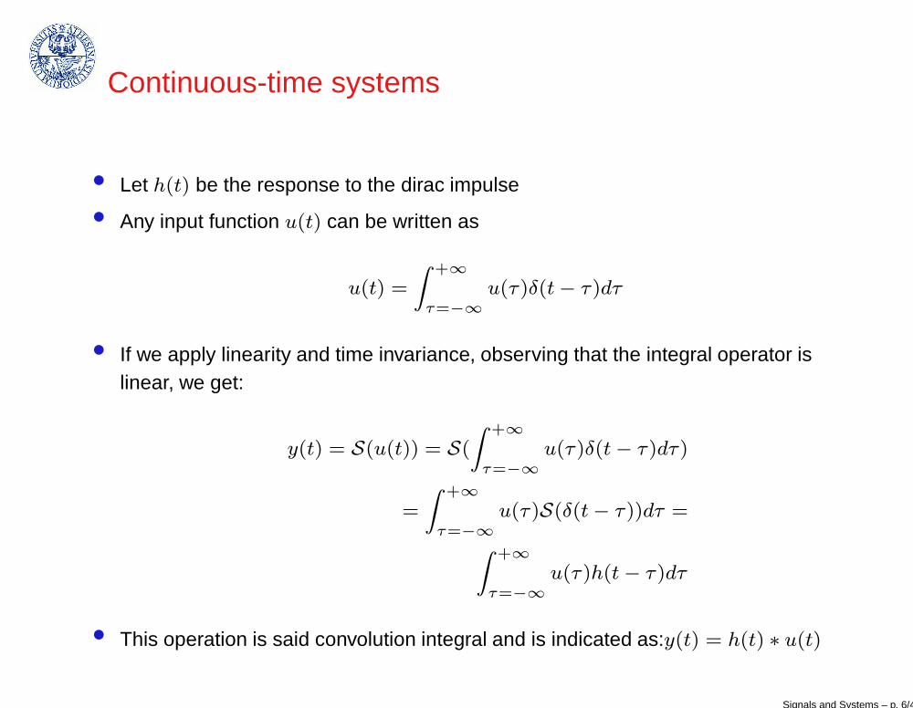
• Let h(t) be the response to the dirac impulse
• Any input function u(t) can be written as
u(t) =
Z +∞
τ=−∞
u(τ)δ(t − τ)dτ
• If we apply linearity and time invariance, observing that the integral operator islinear, we get:
y(t) = S(u(t)) = S(
Z +∞
τ=−∞
u(τ)δ(t − τ)dτ)
=
Z +∞
τ=−∞
u(τ)S(δ(t − τ))dτ =
Z +∞
τ=−∞
u(τ)h(t − τ)dτ
• This operation is said convolution integral and is indicated as:y(t) = h(t) ∗ u(t)
Signals and Systems – p. 6/43
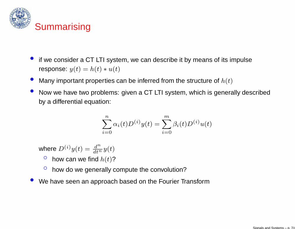
Summarising
• if we consider a CT LTI system, we can describe it by means of its impulseresponse: y(t) = h(t) ∗ u(t)
• Many important properties can be inferred from the structure of h(t)
• Now we have two problems: given a CT LTI system, which is generally describedby a differential equation:
nX
i=0
αi(t)D(i)y(t) =
mX
i=0
βi(t)D(i)u(t)
where D(i)y(t) = dn
dtn y(t)
◦ how can we find h(t)?◦ how do we generally compute the convolution?
• We have seen an approach based on the Fourier Transform
Signals and Systems – p. 7/43

Limitations of the Fourier Approach
• We have already studied the Fourier Transform and we have seen that it allows usto easily study:◦ the response to periodic signals◦ the forced evolution for a class of signals (those for which it is possible to
compute the Fourier Transform)
• However, there is a couple of hidden assumption:◦ the system has to have zero initial conditions◦ the system has to be BIBO stable
Signals and Systems – p. 8/43
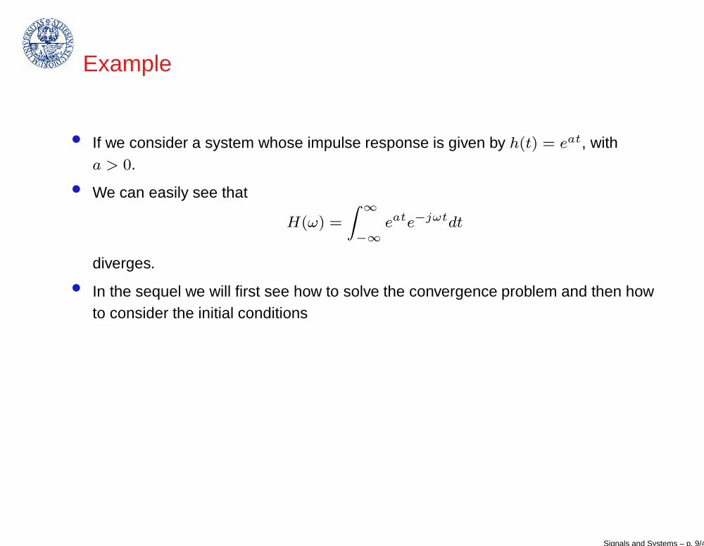
Example
• If we consider a system whose impulse response is given by h(t) = eat, witha > 0.
• We can easily see that
H(ω) =
Z
∞
−∞
eate−jωtdt
diverges.
• In the sequel we will first see how to solve the convergence problem and then howto consider the initial conditions
Signals and Systems – p. 9/43

The Laplace transform
Signals and Systems – p. 10/43
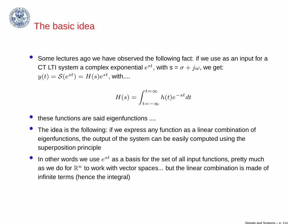
The basic idea
• Some lectures ago we have observed the following fact: if we use as an input for aCT LTI system a complex exponential est, with s = σ + jω, we get:y(t) = S(est) = H(s)est, with....
H(s) =
Z t=∞
t=−∞
h(t)e−stdt
• these functions are said eigenfunctions ....
• The idea is the following: if we express any function as a linear combination ofeigenfunctions, the output of the system can be easily computed using thesuperposition principle
• In other words we use est as a basis for the set of all input functions, pretty muchas we do for R
n to work with vector spaces... but the linear combination is made ofinfinite terms (hence the integral)
Signals and Systems – p. 11/43

Definition
• Given any function u(t), its bilateral Laplace transform is given by:
U(s) =
Z
∞
t=−∞
u(t)e−stdt
• This is called bi-lateral Laplace transform (because t runs from −∞ to ∞). For themono-lateral Laplace -transform the index runs from 0− = limǫ→0 0 − ǫ Clearlythe two transforms coincide for causal signals...
• The Laplace transform is an operator that transforms a functionu(t) into a functionU(s) = L (u(t))
• For the bilateral Laplace Transform we need to address the following issues:
1. U(s) is an integral defined over an infinite domain...For which values of s inthe complex plane does it converge? This region is called region ofconvergence.
2. What type of properties does the L - transform enjoy and what type ofoperations can we do with it?
3. Should this Laplace transform be *really* handy for our purposes, how can wego back (inverse transform)?
Signals and Systems – p. 12/43

Region of Convergence (ROC) – An example
• Let us start from an example...
• Consider the signal u(t) = 1(t)e−at with a real
• The definition of the L - tranform leads us to:
U(s) =
Z
∞
t=−∞
1(t)e−ate−stdt =
Z
∞
t=0e−(s+a)tdt
• A standard results from analysis tells us that this integral converges ifflimt→∞ e−(s+a)t = 0, which, in turn requires Re(s + a) > 0, i.e., Re(s) > −a
• this is the half plan on the right of −a
Signals and Systems – p. 13/43

Region of Convergence (ROC) – An example
• If we are inside the ROC, we can see:
Re(s) > −a → U(s) =
Z
∞
t=0e−(s+a)tdt =
1
s + a
• Now, consider the function: u1(t) = e−at1(−t). Following the same line ofreasoning we find out:
U1(s) =1
s + a, Re(s) < −a
• the two signals have the same Laplace transform but different ROC. So we have toassociate to each signal both the Laplace transform and the ROC.
Signals and Systems – p. 14/43
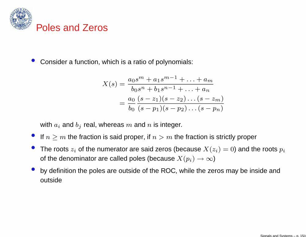
Poles and Zeros
• Consider a function, which is a ratio of polynomials:
X(s) =a0sm + a1sm−1 + . . . + am
b0sn + b1sn−1 + . . . + an
=a0
b0
(s − z1)(s − z2) . . . (s − zm)
(s − p1)(s − p2) . . . (s − pn)
with ai and bj real, whereas m and n is integer.
• If n ≥ m the fraction is said proper, if n > m the fraction is strictly proper
• The roots zi of the numerator are said zeros (because X(zi) = 0) and the roots pi
of the denominator are called poles (because X(pi) → ∞)
• by definition the poles are outside of the ROC, while the zeros may be inside andoutside
Signals and Systems – p. 15/43
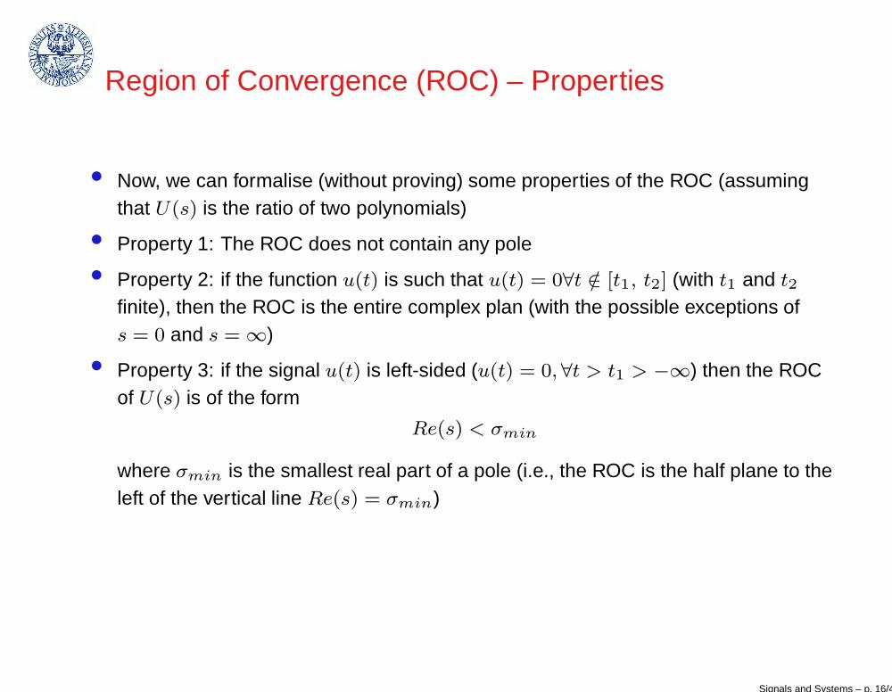
Region of Convergence (ROC) – Properties
• Now, we can formalise (without proving) some properties of the ROC (assumingthat U(s) is the ratio of two polynomials)
• Property 1: The ROC does not contain any pole
• Property 2: if the function u(t) is such that u(t) = 0∀t /∈ [t1, t2] (with t1 and t2
finite), then the ROC is the entire complex plan (with the possible exceptions ofs = 0 and s = ∞)
• Property 3: if the signal u(t) is left-sided (u(t) = 0,∀t > t1 > −∞) then the ROCof U(s) is of the form
Re(s) < σmin
where σmin is the smallest real part of a pole (i.e., the ROC is the half plane to theleft of the vertical line Re(s) = σmin)
Signals and Systems – p. 16/43
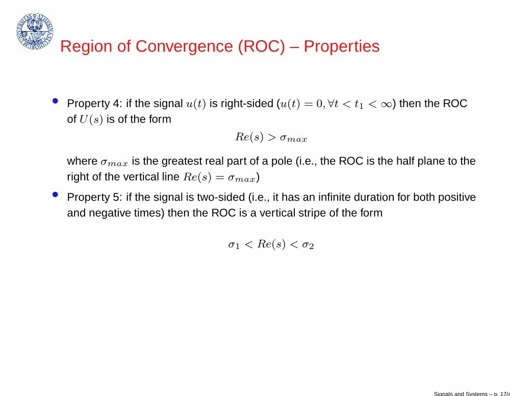
Region of Convergence (ROC) – Properties
• Property 4: if the signal u(t) is right-sided (u(t) = 0, ∀t < t1 < ∞) then the ROCof U(s) is of the form
Re(s) > σmax
where σmax is the greatest real part of a pole (i.e., the ROC is the half plane to theright of the vertical line Re(s) = σmax)
• Property 5: if the signal is two-sided (i.e., it has an infinite duration for both positiveand negative times) then the ROC is a vertical stripe of the form
σ1 < Re(s) < σ2
Signals and Systems – p. 17/43

Some Laplace tranforms
• u(t) = δ(t), Dirac delta;
• L (δ(t)) =∫ ∞t=−∞ δ(t)e−stdt = e−s0 = 1
• hence L(δ(t)) = 1 and the ROC is all s
Signals and Systems – p. 18/43
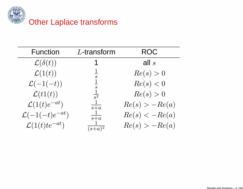
Other Laplace transforms
Function L-transform ROC
L(δ(t)) 1 all s
L(1(t)) 1s Re(s) > 0
L(−1(−t)) 1s Re(s) < 0
L(t1(t)) 1s2 Re(s) > 0
L(1(t)e−at) 1s+a Re(s) > −Re(a)
L(−1(−t)e−at) 1s+a Re(s) < −Re(a)
L(1(t)te−at) 1(s+a)2 Re(s) > −Re(a)
Signals and Systems – p. 19/43
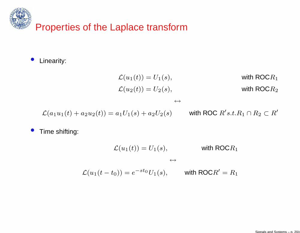
Properties of the Laplace transform
• Linearity:
L(u1(t)) = U1(s), with ROCR1
L(u2(t)) = U2(s), with ROCR2
↔
L(a1u1(t) + a2u2(t)) = a1U1(s) + a2U2(s) with ROC R′s.t.R1 ∩ R2 ⊂ R′
• Time shifting:
L(u1(t)) = U1(s), with ROCR1
↔
L(u1(t − t0)) = e−st0U1(s), with ROCR′ = R1
Signals and Systems – p. 20/43

Properties of the Laplace transform
• Shifiting in the s domain
L(u1(t)) = U1(s), with ROCR1
↔
Z(es0tu1(t)) = U1(s − s0) with ROC R′ = Re(s0) + R1
• Time scaling
L(u1(t)) = U1(s), with ROCR1
↔
L(u1(at)) =1
|a|U1(
s
a) with ROC R = aR1
Signals and Systems – p. 21/43

Properties of the Laplace transform
• Differentiation in the time domain:
L(u1(t)) = U1(s), with ROCR1
↔
L(du1
dt) = sU1(s) with ROC R′ such that R1 ⊂ R′
• Differentiation in the s domain:
L(u1(t)) = U1(s), with ROCR1
↔
L(−tu1(t)) =dU1(s)
dswith ROC R = R1
Signals and Systems – p. 22/43

Properties of the Laplace transform
• Integration
L(u1(t)) = U1(s), with ROCR1
↔
L(
Z t
t=−∞
u(τ)dτ) =1
sU1(s) with ROC R′ = R1 ∩ {Re(s) > 0}
• Convolution
L(u1(t)) = U1(s), with ROCR1
Lt(u2(t)) = U2(s), with ROCR2
↔
L(u1 ∗ u2) = U1(s)U2(s) with ROC R′ such that R1 ∩ R2 ⊂ R′
• the last property is of the greatest practical relevance...a very complex operation(the convolution) has become a staightforward operation) becomes a product
Signals and Systems – p. 23/43

Methodology
• Suppose we want to compute y(t) = h(t) ∗ u(t)
• we compute the Laplace transforms H(s), U(s)
• we compute Y (s) = H(s)U(s)
• we compute the inverse transform of Y (s)
Signals and Systems – p. 24/43

The unilateral Laplace transform
• For the unilateral Laplace transform the in is carried over positive times
U(s) =
Z +∞
0−u(t)e−stdt
The integration from 0− allows to embrace the dirac δ
• The unilateral Laplace transform is equivalent to the Laplace transform of 1(t) u(t).Therefore, the ROC is always of the form Re(s) > σmax.
• Most of the properties of the bilateral transform also apply to mono-lateral Laplacetransform
• The differentiation property is modified as follows L(u(t)) = U(s) ↔
L(dnu(t)
dtn) = snU(s) − sn−1u(0−) − sn−2u′(0−) − . . . − u(n−1)(0−)
with u(n−1)defined asdnu(t)
dtn
• This property is particularly useful to take into account the initial conditions forcausal systems to causal inputs (it allows to compute the unforced evolution)
Signals and Systems – p. 25/43

Computation of the Laplace transform
• One possible way to do this is via a direct application of the definition
• Another possibility is to use the Laplace transform of known functions and applythe properties
• For instance, suppose we want to find the Laplace transform ofu(t) = teat1(t) + 1(t − t0)ea(t−t0)
• Applying linearity we get L(u(t)) = L(1(t − t0)ea(t−t0)) + L(teat1(t))
• Applying the time shifting property:
L(eat1(t)) =1
s − a→ L(ea(t−t0)1(t − t0)) = e−st0
1
s − a
L(teat1(t)) =1
(s − a)2
• Therefore U(s) =“
1(s−a)2
+ e−st0 1(s−a)
”
Signals and Systems – p. 26/43

Computation of the transfer function
• Consider a causal LTI system described by
npX
j=0
ajy(j)(t) =
nzX
j=0
bju(j)(t).
Suppose u is a causal signal. By u(i) we mean u(t) derived i times.
• if we compute the Laplace transform of both terms we get
npX
j=0
ajsjY (s) −
npX
j=1
ajsj−1y(0−) − . . . +
npX
j=np−1
ajsj−1y(np−2)(0−) − anpy(np−1)(0−) =
=
nzX
j=0
bjsjU(s) −
nzX
j=1
bjsj−1u(0−) − . . . +
−
nzX
j=nz−1
bjsj−1u(nz−2)(0−) − bnz u(nz−1)(0−)
Signals and Systems – p. 27/43

Computation of the transfer function (continued)
• Hence,
Y (s) =
Pnzj=0
bjsj
Pnpj=0
ajsjU(s)+
1Pnp
j=0ajsj
“
Pnp
j=1 ajsj−1y(0−) + . . . + anpy(np−1)(0−)+
−Pnz
j=1 bjsj−1u(0−) − . . . − bnz u(nz−1)(0−)”
• Therefore,
y(t) = L−1
„
Pnzj=0
bjsj
Pnpj=0
ajsjU(s)
«
+
+L−1
„
1Pnp
j=0ajsj
“
Pnp
j=1 ajsj−1y(0−) + . . . + anpy(np−1)(0−)”
«
+
−L−1
„
1Pnp
j=0ajsj
“
Pnzj=1 bjsj−1u(0−) + . . . + bnz u(nz−1)(0−)
”
«
• Once again, we found a forced and an unforced response...
Signals and Systems – p. 28/43

Transfer function
• if we consider initial conditions equal to 0 then
Y (s) = H(s)U(s), with H(s) =Pnz
j=0bjsj
Pnp
j=0ajsj
• H(s) is the L-transform of the impulse response and it iscalled transfer function
• Indeed, the convolution y(t) = h(n) ∗ u(t) corresponds to aproduct in the s domain
• Now, it is time to study how to compute the inversetransform of the L-transform
• In particular it is important to look at fractions of polynomials
Signals and Systems – p. 29/43

Computation of the inverse L-transform
• Let us start from a simplified situation:
X(s) =N(s)
D(s)= k
(s − z1) . . . (s − zm)
(s − p1) . . . (s − pn)
in which n ≥ m and all poles pk are simple (i.e., they have algebraic multiplicityequal to 1)
• We can do the so-called partial fraction expansion then set
X(s) =c1
s − p1+ . . . +
cn
s − pn
where
c1 = (s − p1)X(s)|s=p1
. . .
cn = (s − pn)X(s)|s=pn
• For mono-lateral L we can compute the inverse transform as considering that:L{epit} = 1
s−pi
Signals and Systems – p. 30/43

Computation of the inverse L-transform
• In case of multiple roots, we proceed as before except that we have more than onepartial fraction for the multiple root:
X(s) = k(s − z1) . . . (s − zm)
(s − p1)(s − pi)h . . . (s − pn)
↔
X(s) = c11
s − p1+ . . . + c
(1)i
1
s − pi
+ c(2)i
1
(s − pi)2+ . . . + c
(h)i
1
(s − pi)h+
+ . . . + cn1
s − pn
• For mono-lateral L we have:
L{epit} =1
s − pi
L{tnepit} =n!
(s − pi)n+1
Signals and Systems – p. 31/43
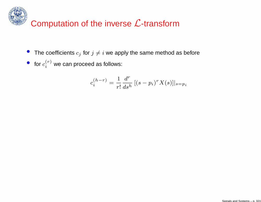
Computation of the inverse L-transform
• The coefficients cj for j 6= i we apply the same method as before
• for c(r)i we can proceed as follows:
c(h−r)i =
1
r!
dr
dsh[(s − pi)
rX(s)]|s=pi
Signals and Systems – p. 32/43

Properties of the signal readable from the
unilateral L• If all poles are strictly in the left half plane (∀i Re(pi) < 0) then goes to 0 for t → ∞
• If one of the poles is in the right half plane (∃i Re(pi) > 0) becomes unbounded ast → ∞
• If all poles are such that Re(pi) ≤ 0, then if all poles with real part equal to zeroare simple then the functions remains bounded (although it does not necessarilygo to 0), otherwise the function is unbounded.
• Initial value theorem: u(0) = lims→∞ sU(s)
• Final value theorem: u(∞) = lims→0 sU(s) (if the limit exists and is finite).
Signals and Systems – p. 33/43

Example 3
• Consider the following system:
y(t) + 0.5y(t) = u(t) − 3u(t)
• Assume u(0) = 1, y(0) = −3. Compute the response to a step input
• Both the input signal and the transfer function are causal (y(t) does not depend ont). Hence, we use the monolateral L-transform
• We can apply the rule L(y) = sY (s) − y(0−), and L(u) = sU(s) − u(0−)
Signals and Systems – p. 34/43

Example 3 – Continued
• Therefore, sY (s) − y(0) + 0.5Y (s) = U(s) − 3sU(s) − 3u(0−)
• ... andY (s)(s + 0.5) = U(s)(−3s + 1) + (y(0−) − 3u(0−))
Y (s) =−3s + 1
s + 0.5U(s) −
6
s + 0.5
The transfer function is H(s) = −3s+1s+0.5
• Now, U(s) = 1s
therefore
Y (z) =−3s + 1
(s + 0.5)s−
6
s + 0.5
Signals and Systems – p. 35/43

Example 3 – Continued
• We compute the inverse transform of each piece.
• The part related to the initial conditions is very easy:
L−1(1
s + 05) = 1(t)e−0.5t
• For the forced response we have to to the partial fractions expansionsYf (s) = H(s)U(s):
Yf (s) =−3s + 1
s(s + 0.5)=
2
s−
5
s + 0.5
Signals and Systems – p. 36/43
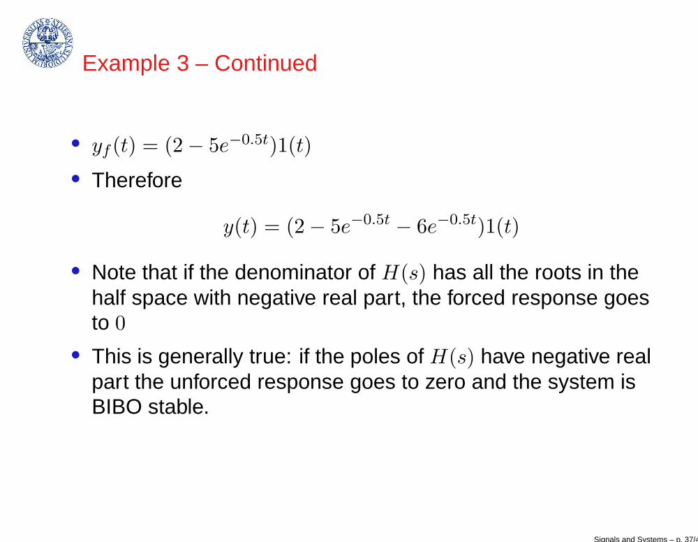
Example 3 – Continued
• yf (t) = (2 − 5e−0.5t)1(t)
• Therefore
y(t) = (2 − 5e−0.5t − 6e−0.5t)1(t)
• Note that if the denominator of H(s) has all the roots in thehalf space with negative real part, the forced response goesto 0
• This is generally true: if the poles of H(s) have negative realpart the unforced response goes to zero and the system isBIBO stable.
Signals and Systems – p. 37/43

Characterisation of the transfer function
• We have seen that (with 0 initial conditions) we have got
y(t) = h(t) ∗ u(t)
↔
Y (s) = H(s)U(s)
where h(t) is the impulse response and H(s) is the transfer function.
• Causality: h(t), t < 0. Since the impulse response is right-sided, then the ROC ofH(s) has to be Re(s) > smax
• BIBO stability: we have seen that it corresponds toR +∞
t=−∞|h(t)|dt ≤ ∞. This
corresponds to the ROC containing the line Re(s) = 0.
• if the system is both causal and BIBO stable , it must have all the poles inside the left
half plane Re(pi) < 0 for all pi
Signals and Systems – p. 38/43
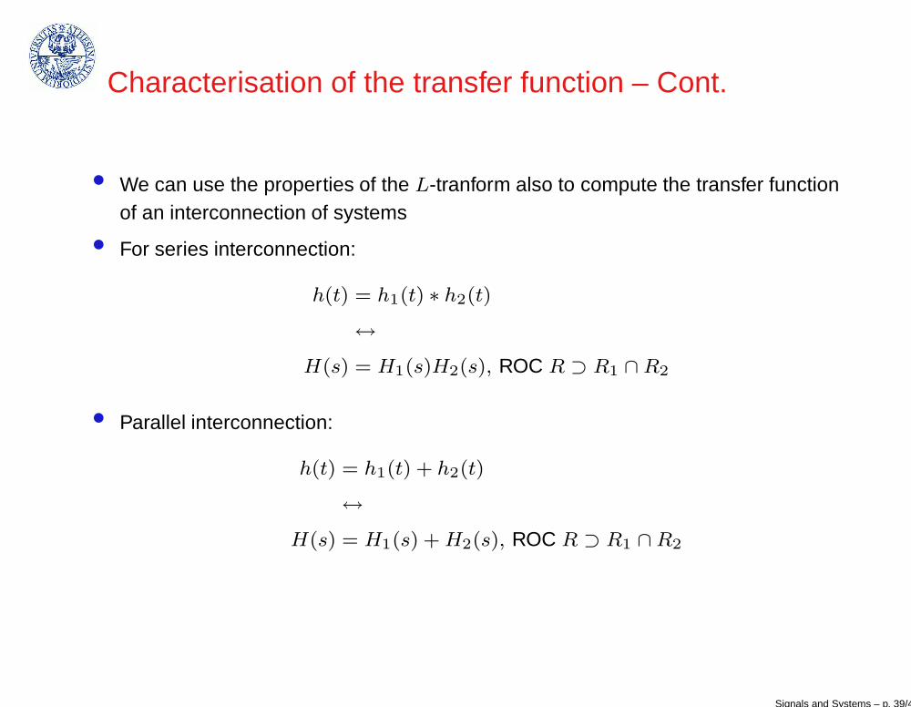
Characterisation of the transfer function – Cont.
• We can use the properties of the L-tranform also to compute the transfer functionof an interconnection of systems
• For series interconnection:
h(t) = h1(t) ∗ h2(t)
↔
H(s) = H1(s)H2(s), ROC R ⊃ R1 ∩ R2
• Parallel interconnection:
h(t) = h1(t) + h2(t)
↔
H(s) = H1(s) + H2(s), ROC R ⊃ R1 ∩ R2
Signals and Systems – p. 39/43
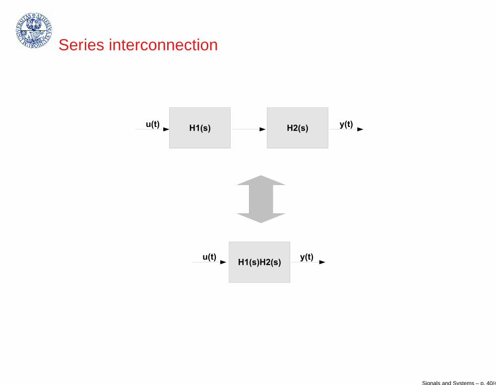
Series interconnection
Signals and Systems – p. 40/43

Parallel interconnection
Signals and Systems – p. 41/43
Characterisation of the transfer function – Cont.
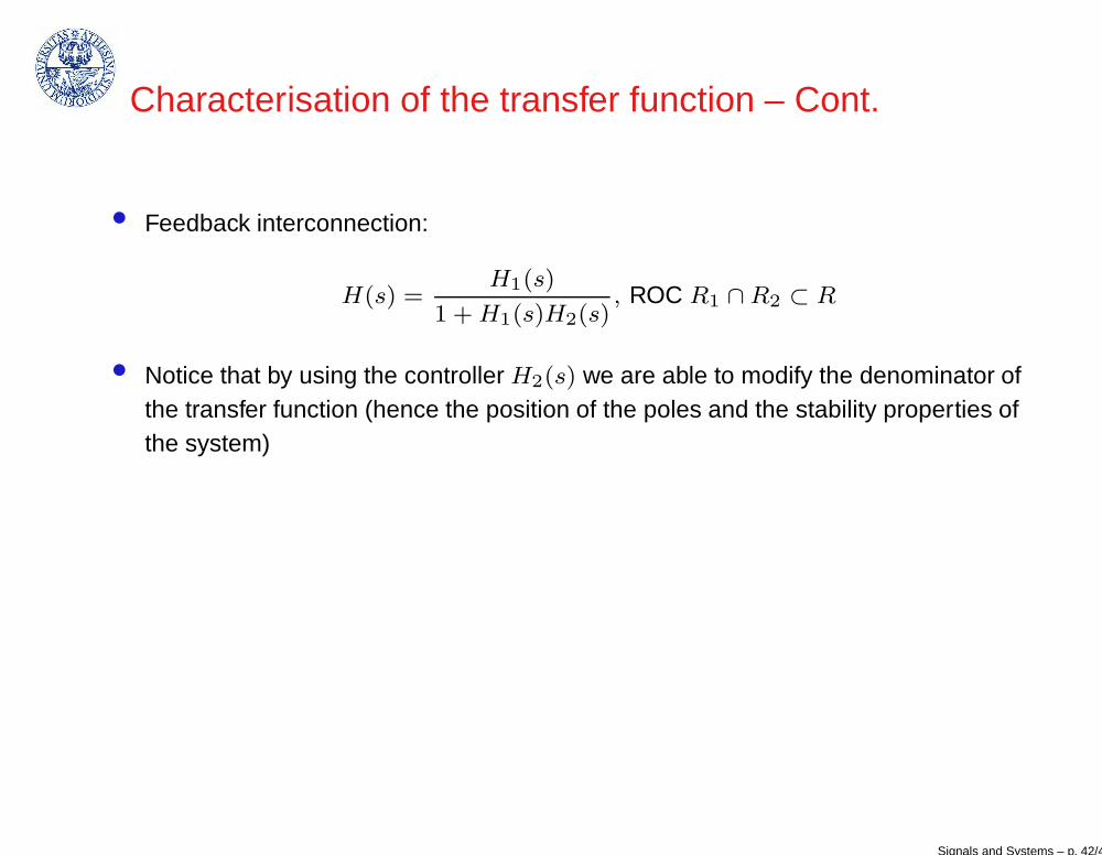
• Feedback interconnection:
H(s) =H1(s)
1 + H1(s)H2(s), ROC R1 ∩ R2 ⊂ R
• Notice that by using the controller H2(s) we are able to modify the denominator ofthe transfer function (hence the position of the poles and the stability properties ofthe system)
Signals and Systems – p. 42/43

Feedback interconnection
Signals and Systems – p. 43/43