Signals and Systems - Academic Computer Centeracademic.pgcc.edu/~sjohnson/lecture1_egr205.pdf ·...
18
Signals and Systems ● A signal is the representation of a physical “wave” – Expressed as a variable in time-space, for instance x(t) – Signals that might vary are the voltage or current of a circuit, the force in a mechanical circuit, heat flow in a thermal circuit, or hydraulic flow in a fluid circuit ● A system is a process that has as an input a signal and outputs a different signal (usually)
Transcript of Signals and Systems - Academic Computer Centeracademic.pgcc.edu/~sjohnson/lecture1_egr205.pdf ·...

Signals and Systems
● A signal is the representation of a physical “wave”– Expressed as a variable in time-space, for
instance x(t)– Signals that might vary are the voltage or
current of a circuit, the force in a mechanical circuit, heat flow in a thermal circuit, or hydraulic flow in a fluid circuit
● A system is a process that has as an input a signal and outputs a different signal (usually)

Signals and Systems
● A system is a process that has as an input a signal and outputs a different signal (usually)– Expressed as a transfer function or an
operator– As an example an operator could be an
integrator taking a signal and integrating over time, or it could be just as simple as multiplying by a constant

Signals and Systems
● The methods that are used in signals and systems are in general the same methods learned in linear algebra
● However this is only part of the story...the analytic part
● The other part of the story on how to actually model these and use them in the real world requires an introduction to numerical methods

Numerical Methods
● Methods of approximating physical problems that are intractable using analytic techniques– Physical problems are represented by
mathematical equations– A number of approximation techniques for
the same physical expression are used depending on the situation
● Methods of assigning error to approximated solutions
Numerical Methods
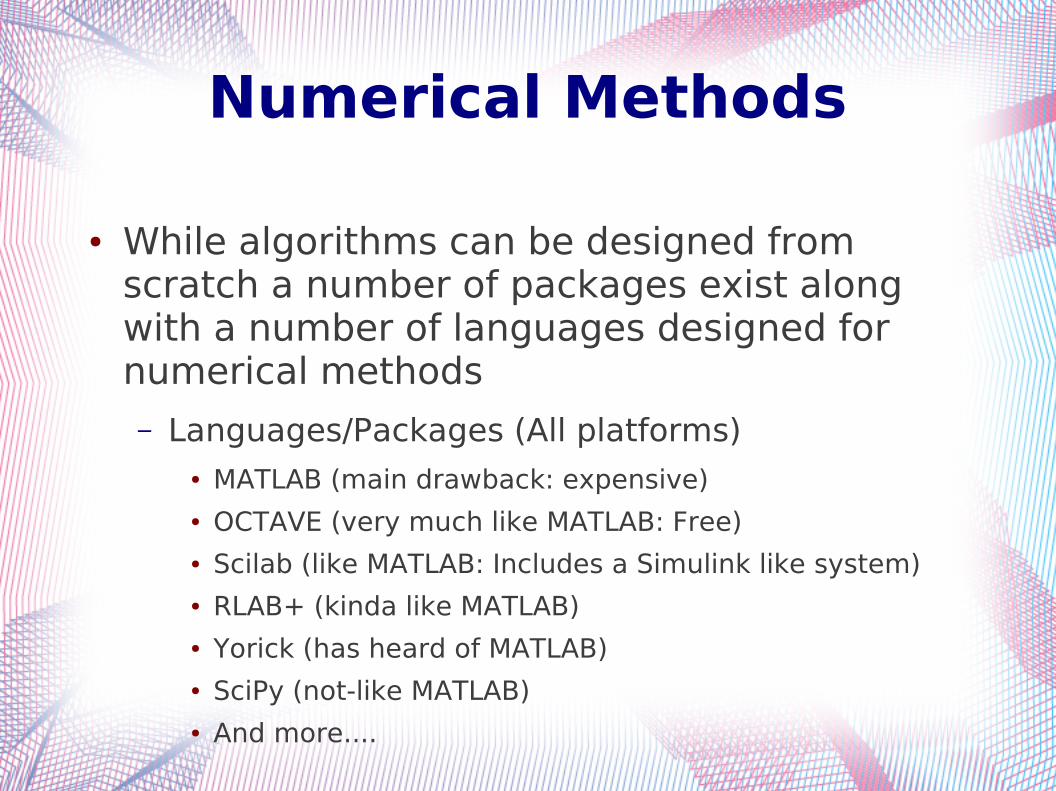
● While algorithms can be designed from scratch a number of packages exist along with a number of languages designed for numerical methods– Languages/Packages (All platforms)
● MATLAB (main drawback: expensive)● OCTAVE (very much like MATLAB: Free)● Scilab (like MATLAB: Includes a Simulink like system)● RLAB+ (kinda like MATLAB)● Yorick (has heard of MATLAB)● SciPy (not-like MATLAB)● And more....

Numerical Methods
● Continued– Packages (almost always in Fortran though C
translations do exist for most and some JAVA)● LINPACK: Linear algebra pack● LAPACK: Modern linear algebra pack● MINPACK: non-linear problems● ODEPACK: Differential equations● QUADPACK: Integration, etc.● FFTPACK: FFTs, of course● SLAP: Sparse Linear Algebra Package● BLAS: Basic Linear Algebra subprograms● Many more (see list at NETLIB on web site)
Numerical Methods
● Continued– For Java numerical methods routines go to
http://math.nist.gov/javanumerics/

Numerical Methods
● Packages are compiled and made libraries– EGR205% gcc -c -O2 test.f
– EGR205% gcc test.o -lm -lc -lslap -lblas -o test
– EGR205% ./test● Program gives output of some sort● Example of subroutine used in say “slap” might
be sgmres (see handout) which is a preconditioned GMRES (generalized minimum residual) iterative sparse Ax=b solver

Numerical Methods
● Getting MATLAB– http://www.mathworks.com/products/matlab/– http://www.mathworks.com/academia/student_version/
● Getting OCTAVE
– http://www.gnu.org/software/octave/– For windows (sourceforge is best)
● http://octave.sourceforge.net/–http://www.cygwin.com/– http://academic.pgcc.edu/~sjohnson/cygwintut.html
● This gives step-by-step instructions on placing cygwin WITH octave on your system

Numerical Methods● Second law and the parachuting person
● F = ma
● F = F_d + F_u– F_d = mg
– F_u = -cv2
● Therefore the analytic from is converted to digital form– dv/dt = (mg – cv2)/m = g – cv2/m
● [v(i+1)-v(i)]/[t(i+1)-t(i)] = g – cv(i)2/m● v(i+1)=v(i) + [g-cv(i)2/m]*[t(i+1)-t(i)]
● Try programming and running this at home
Numerical Methods
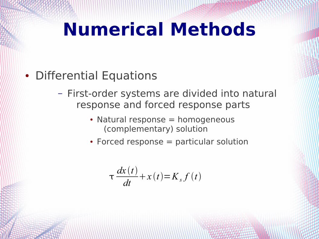
● Differential Equations– First-order systems are divided into natural
response and forced response parts● Natural response = homogeneous
(complementary) solution● Forced response = particular solution
dx t dt
x t =K s f t

Numerical Methods
● Natural Solution first
dxn t
dtx t =0
dxn t
dt=
−xn t
dxn t = e−t /
∫dxn t
dt=−∫ dt
xn t =e−t / ec
xn t = e−t /

Numerical Methods
● Forced solution– Assume a constant force response
(otherwise it is harder)
dx f t
dtx t =K sF
dx f t =K sF for t0
Numerical Methods
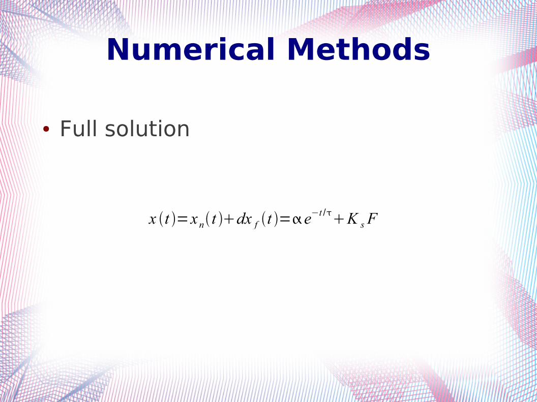
● Full solution
x t =xn t dx f t = e−t /K sF

Writing good program
● Pseudocode– Pretty much English in the manner you like
● If/then/else● Case● Do while● Do until● Do for i=a,b,step● End● etc
● Flowcharts

Flowchart Symbols
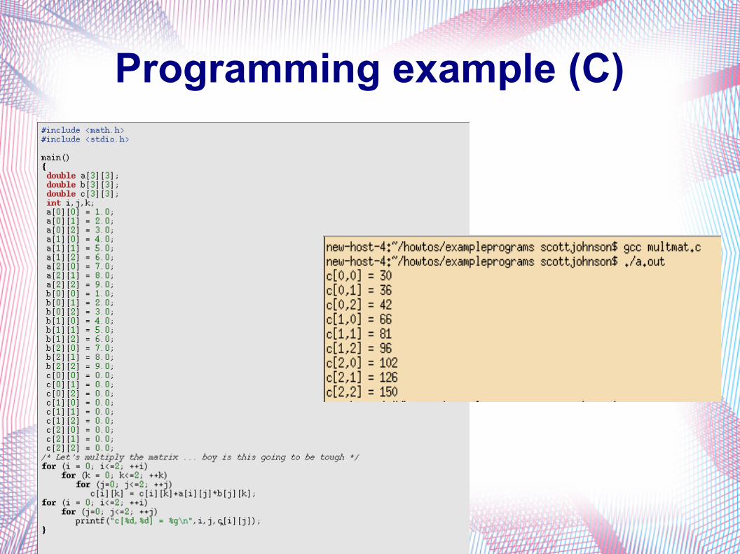
Programming example (C)

Programming example (Matlab)