Signal Processing Methodologies for Resource-E … Processing Methodologies for Resource-E cient and...
187
Signal Processing Methodologies for Resource-Efficient and Secure Communications in Wireless Networks by Francis Minhthang Bui A thesis submitted in conformity with the requirements for the degree of Doctor of Philosophy Graduate Department of Electrical and Computer Engineering University of Toronto c Copyright by Francis Minhthang Bui, 2009
Transcript of Signal Processing Methodologies for Resource-E … Processing Methodologies for Resource-E cient and...

Signal Processing Methodologies for
Resource-Efficient and Secure Communications
in Wireless Networks
by
Francis Minhthang Bui
A thesis submitted in conformity with the requirementsfor the degree of Doctor of Philosophy
Graduate Department of Electrical and Computer EngineeringUniversity of Toronto
c© Copyright by Francis Minhthang Bui, 2009

Signal Processing Methodologies for Resource-Efficient and Secure
Communications in Wireless Networks
Francis Minhthang Bui
Doctor of Philosophy, 2009
Graduate Department of Electrical and Computer Engineering
University of Toronto
Abstract
Future-generation wireless and mobile networks are expected to support a panoply of multimedia
services, ranging from voice to video data. There is also a de facto ”anytime anywhere” mentality that
reliable communications should be ubiquitously guaranteed, irrespective of temporal or geographical
constraints. However, the implicit catch is that these specifications should be achieved with only mini-
mal infrastructure expansion or cost increases. In this thesis, various signal processing methodologies
conducive to attaining these goals are presented.
First, a system model that takes into account the time-varying nature of the mobile environment
is developed. To this end, a mathematically tractable basis-expansion model (BEM) of the commu-
nication channel, augmented with multiple-state characterization, is proposed. In the context of the
developed system model, strategies for enhancing the quality of service (QoS), while maintaining
resource efficiency, are then studied. Specifically, dynamic channel tracking, adaptive modulation and
coding, interpolation and random sampling, and spatiotemporal processing are examined as enabling
solutions. Next, the question of how to appropriately aggregate these disparate methods is recast as
a nonlinear constrained optimization problem. This enables the construction of a flexible framework
that can accommodate a wide range of applications, to deliver practical network designs. In par-
ticular, the developed methods are well-suited for multi-user communication systems, implemented
using spread-spectrum and multi-carrier solutions, such as code division multiple access (CDMA)
and orthogonal frequency division multiplexing (OFDM).
Moreover, privacy and security requirements are increasingly becoming essential aspects of the
QoS paradigm in communications. Combined with the advent of novel security technologies, such
as biometrics, the conventional communication infrastructure is expected to undergo fundamental
ii

modifications to support these new system components and modalities. Therefore, within the same
framework for maximizing resource efficiency, several unique signal processing applications in net-
work security using biometrics are also investigated in this thesis. It is shown that a resource allocation
approach is equally appropriate, and productive, in delivering efficient and practical key distribution
and biometric encryption solutions for secure communications.
iii

Dedication
To my family.
iv

Acknowledgements
My sincere gratitude must first go to my advisor, Prof. Dimitrios Hatzinakos, for his guidance,
encouragement, and confidence in me throughout my graduate studies. His patience, expertise, and
insightful leadership have engendered an ambience that is tremendously conducive to research and
innovations in the Multimedia Research Group.
I would like to also acknowledge my thesis committee Professors Frank Kschischang, Kostas
Plataniotis, Teng Joon Lim and Sridhar Krishnan for their perspicacious feedback on this thesis. In
addition, I am indebted to the Natural Sciences and Engineering Research Council of Canada, and the
Government of Ontario for the generous financial funding of my research work.
Last but not least, I wish to give my wholehearted thanks to my family for their unconditional
support and infinite understanding. Mom, dad, Thomas, and Avy: your care, empathy and love
have rendered even my most adverse challenges in life bearable, and have made all my struggles and
endeavors worthwhile.
v

Contents
Abstract ii
Dedication iv
Acknowledgements v
List of Figures xiii
List of Tables xiv
List of Abbreviations xv
1 Background and Motivations 1
1.1 Resources and Constraints in Wireless and Mobile Networks . . . . . . . . . . . . . . . . 1
1.2 Methods for Regulating the Quality of Service . . . . . . . . . . . . . . . . . . . . . . . . 3
1.3 Summary of Thesis Contributions . . . . . . . . . . . . . . . . . . . . . . . . . . . . . . . 5
1.3.1 List of Publications . . . . . . . . . . . . . . . . . . . . . . . . . . . . . . . . . . . . 7
2 System Modeling and Identification 8
2.1 Established Works . . . . . . . . . . . . . . . . . . . . . . . . . . . . . . . . . . . . . . . . . 8
2.1.1 Statistical Channel Characterization . . . . . . . . . . . . . . . . . . . . . . . . . . 9
2.1.2 Rayleigh Fading Channel . . . . . . . . . . . . . . . . . . . . . . . . . . . . . . . . 11
2.1.3 Discrete-Time Channel Modeling . . . . . . . . . . . . . . . . . . . . . . . . . . . . 12
2.1.4 Basis-Expansion Channel Modeling . . . . . . . . . . . . . . . . . . . . . . . . . . 14
2.1.5 Quasi-Static Modeling and Fixed-Size Block Transceivers . . . . . . . . . . . . . . 15
2.2 Variable-Size Block-Based Transceivers: Signal Models and Notations . . . . . . . . . . . 16
2.2.1 Contributions . . . . . . . . . . . . . . . . . . . . . . . . . . . . . . . . . . . . . . . 16
2.2.2 Multiple-State Channel Modeling . . . . . . . . . . . . . . . . . . . . . . . . . . . 17
vi

2.2.3 Time-Invariant Block Processing . . . . . . . . . . . . . . . . . . . . . . . . . . . . 18
2.2.4 Time-Variant Block Processing . . . . . . . . . . . . . . . . . . . . . . . . . . . . . 28
2.3 Channel Identification for Variable-Size Block Systems . . . . . . . . . . . . . . . . . . . 30
2.3.1 Contributions . . . . . . . . . . . . . . . . . . . . . . . . . . . . . . . . . . . . . . . 30
2.3.2 Channel Identification for Time-Invariant Block Processing . . . . . . . . . . . . . 31
2.3.3 Channel Identification for Time-Variant Block Processing . . . . . . . . . . . . . . 32
2.4 Summary . . . . . . . . . . . . . . . . . . . . . . . . . . . . . . . . . . . . . . . . . . . . . . 34
3 Adaptation Methods for QoS Regulation 35
3.1 Quality of Service (QoS) Metrics: A Brief Survey . . . . . . . . . . . . . . . . . . . . . . . 36
3.2 Channel Tracking and Block-Size Adaptation . . . . . . . . . . . . . . . . . . . . . . . . . 38
3.2.1 Motivations and Previous Works . . . . . . . . . . . . . . . . . . . . . . . . . . . . 38
3.2.2 Contributions . . . . . . . . . . . . . . . . . . . . . . . . . . . . . . . . . . . . . . . 41
3.2.3 Variable-Size Block Structure . . . . . . . . . . . . . . . . . . . . . . . . . . . . . . 42
3.2.4 Channel Tracking for Variable-Size Block Construction . . . . . . . . . . . . . . . 45
3.3 Adaptive Modulation . . . . . . . . . . . . . . . . . . . . . . . . . . . . . . . . . . . . . . . 48
3.3.1 Motivations and Previous Works . . . . . . . . . . . . . . . . . . . . . . . . . . . . 48
3.3.2 Contributions . . . . . . . . . . . . . . . . . . . . . . . . . . . . . . . . . . . . . . . 50
3.3.3 Channel Metrics . . . . . . . . . . . . . . . . . . . . . . . . . . . . . . . . . . . . . 50
3.3.4 Threshold-Based Mode Adaptation . . . . . . . . . . . . . . . . . . . . . . . . . . 54
3.3.5 Selection of Thresholds . . . . . . . . . . . . . . . . . . . . . . . . . . . . . . . . . 54
3.3.6 Integration with Variable-Size Block Construction . . . . . . . . . . . . . . . . . . 55
3.4 PAPR Reduction: An INTRES Approach . . . . . . . . . . . . . . . . . . . . . . . . . . . . 55
3.4.1 Motivations and Previous Works . . . . . . . . . . . . . . . . . . . . . . . . . . . . 55
3.4.2 Contributions . . . . . . . . . . . . . . . . . . . . . . . . . . . . . . . . . . . . . . . 57
3.4.3 System Assumptions and Definitions . . . . . . . . . . . . . . . . . . . . . . . . . 57
3.4.4 INTRES Transmitter Structure . . . . . . . . . . . . . . . . . . . . . . . . . . . . . 59
3.4.5 INTRES Receiver Structure . . . . . . . . . . . . . . . . . . . . . . . . . . . . . . . 62
3.4.6 Redundancy and Complexity . . . . . . . . . . . . . . . . . . . . . . . . . . . . . . 64
3.5 Antenna Allocation and Cooperation for Space-Time Processing . . . . . . . . . . . . . . 65
3.5.1 Motivations and Previous Works . . . . . . . . . . . . . . . . . . . . . . . . . . . . 65
3.5.2 Contributions . . . . . . . . . . . . . . . . . . . . . . . . . . . . . . . . . . . . . . . 66
3.5.3 Spatio-Temporal Signal Model . . . . . . . . . . . . . . . . . . . . . . . . . . . . . 67
3.5.4 Antenna Allocation . . . . . . . . . . . . . . . . . . . . . . . . . . . . . . . . . . . . 68
vii

3.5.5 Cooperation and Virtual Antennas: A Potential Extension . . . . . . . . . . . . . 71
3.6 Simulation Results . . . . . . . . . . . . . . . . . . . . . . . . . . . . . . . . . . . . . . . . 72
3.6.1 Channel Tracking and Block-Size Adaptation Performance . . . . . . . . . . . . . 72
3.6.2 Adaptive Modulation Performance . . . . . . . . . . . . . . . . . . . . . . . . . . 75
3.6.3 PAPR Reduction Performance . . . . . . . . . . . . . . . . . . . . . . . . . . . . . 77
3.6.4 Antenna Allocation Performance . . . . . . . . . . . . . . . . . . . . . . . . . . . . 80
3.7 Summary . . . . . . . . . . . . . . . . . . . . . . . . . . . . . . . . . . . . . . . . . . . . . . 81
4 Secure Communications in Resource-Constrained Body-Area Networks 83
4.1 Literature Survey . . . . . . . . . . . . . . . . . . . . . . . . . . . . . . . . . . . . . . . . . 83
4.1.1 Security and Emerging Communication Standards . . . . . . . . . . . . . . . . . 83
4.1.2 The ECG as a Biometric . . . . . . . . . . . . . . . . . . . . . . . . . . . . . . . . . 85
4.1.3 The ECG for Identification . . . . . . . . . . . . . . . . . . . . . . . . . . . . . . . . 85
4.1.4 Network Security Using the ECG Biometric . . . . . . . . . . . . . . . . . . . . . . 86
4.1.5 Body Area Networks . . . . . . . . . . . . . . . . . . . . . . . . . . . . . . . . . . . 86
4.1.6 Resource Constraints in BANs . . . . . . . . . . . . . . . . . . . . . . . . . . . . . 88
4.1.7 Security and Biometrics in BANs . . . . . . . . . . . . . . . . . . . . . . . . . . . . 89
4.1.8 The ECG Biometric in BANs . . . . . . . . . . . . . . . . . . . . . . . . . . . . . . 89
4.1.9 Single-Point Fuzzy Key Management with the ECG Biometric . . . . . . . . . . . 92
4.1.10 Scheduling and System Synchronization . . . . . . . . . . . . . . . . . . . . . . . 93
4.1.11 Channel Models for BANs . . . . . . . . . . . . . . . . . . . . . . . . . . . . . . . . 94
4.2 Key Management in BANs . . . . . . . . . . . . . . . . . . . . . . . . . . . . . . . . . . . . 96
4.2.1 Motivations and Previous Works . . . . . . . . . . . . . . . . . . . . . . . . . . . . 96
4.2.2 Contributions . . . . . . . . . . . . . . . . . . . . . . . . . . . . . . . . . . . . . . . 96
4.2.3 Multi-Point Fuzzy Key Management . . . . . . . . . . . . . . . . . . . . . . . . . . 97
4.2.4 Performance and Efficiency . . . . . . . . . . . . . . . . . . . . . . . . . . . . . . . 101
4.3 INTRAS Data Scrambling . . . . . . . . . . . . . . . . . . . . . . . . . . . . . . . . . . . . 103
4.3.1 Motivations and Previous Works . . . . . . . . . . . . . . . . . . . . . . . . . . . . 103
4.3.2 Contributions . . . . . . . . . . . . . . . . . . . . . . . . . . . . . . . . . . . . . . . 104
4.3.3 Envisioned Domain of Applicability . . . . . . . . . . . . . . . . . . . . . . . . . . 104
4.3.4 INTRAS High-Level Structure . . . . . . . . . . . . . . . . . . . . . . . . . . . . . 105
4.3.5 INTRAS with Linear Interpolators . . . . . . . . . . . . . . . . . . . . . . . . . . . 106
4.3.6 INTRAS with Higher-Order Interpolators . . . . . . . . . . . . . . . . . . . . . . . 110
4.4 Simulation Results . . . . . . . . . . . . . . . . . . . . . . . . . . . . . . . . . . . . . . . . 112
viii

4.4.1 Key Generation and Distribution . . . . . . . . . . . . . . . . . . . . . . . . . . . . 113
4.4.2 Data Scrambling . . . . . . . . . . . . . . . . . . . . . . . . . . . . . . . . . . . . . 114
4.5 Summary . . . . . . . . . . . . . . . . . . . . . . . . . . . . . . . . . . . . . . . . . . . . . . 117
5 Resource Allocation: An Optimization Framework 119
5.1 Established Works in Constrained Optimization . . . . . . . . . . . . . . . . . . . . . . . 119
5.1.1 The Standard Form for Optimization Problems . . . . . . . . . . . . . . . . . . . . 120
5.1.2 Karush-Kuhn-Tucker (KKT) Conditions . . . . . . . . . . . . . . . . . . . . . . . . 121
5.1.3 Numerical Optimization and the Black-Box Problem Description . . . . . . . . . 122
5.1.4 Scalarization for Multi-Objective Problems . . . . . . . . . . . . . . . . . . . . . . 123
5.2 Established Works in Mixed-Integer Optimization . . . . . . . . . . . . . . . . . . . . . . 123
5.2.1 Branch-and-Bound Algorithm . . . . . . . . . . . . . . . . . . . . . . . . . . . . . 124
5.3 Resource Allocation Applications in Wireless Networks . . . . . . . . . . . . . . . . . . . 125
5.3.1 Motivations and Previous Works . . . . . . . . . . . . . . . . . . . . . . . . . . . . 125
5.3.2 Contributions . . . . . . . . . . . . . . . . . . . . . . . . . . . . . . . . . . . . . . . 126
5.3.3 Channel Tracking Application . . . . . . . . . . . . . . . . . . . . . . . . . . . . . 127
5.3.4 Adaptive Modulation Application . . . . . . . . . . . . . . . . . . . . . . . . . . . 128
5.4 Performance Case Studies . . . . . . . . . . . . . . . . . . . . . . . . . . . . . . . . . . . . 131
5.4.1 Channel Tracking Performance . . . . . . . . . . . . . . . . . . . . . . . . . . . . . 131
5.4.2 BEM Channel Tracking Performance . . . . . . . . . . . . . . . . . . . . . . . . . . 133
5.4.3 Adaptive Modulation Performance and Metric Latency Errors . . . . . . . . . . . 135
5.4.4 Performance of an Aggregate Adaptation System . . . . . . . . . . . . . . . . . . 137
5.5 Resource Allocation for Secure BAN Applications . . . . . . . . . . . . . . . . . . . . . . 138
5.5.1 Motivations and Previous Works . . . . . . . . . . . . . . . . . . . . . . . . . . . . 138
5.5.2 Contributions . . . . . . . . . . . . . . . . . . . . . . . . . . . . . . . . . . . . . . . 139
5.5.3 Morphing Encoder and Random Set Optimization . . . . . . . . . . . . . . . . . . 139
5.5.4 Multi-Point Management with Key Fusion Extension . . . . . . . . . . . . . . . . 142
5.5.5 Performance of Data Scrambling with Key Optimization . . . . . . . . . . . . . . 143
5.5.6 Performance of Data Scrambling using Variable-Size Block Construction . . . . . 144
5.5.7 Performance of the Key Fusion Scheme . . . . . . . . . . . . . . . . . . . . . . . . 145
5.6 Summary . . . . . . . . . . . . . . . . . . . . . . . . . . . . . . . . . . . . . . . . . . . . . . 146
6 Conclusion 148
6.1 General Summary . . . . . . . . . . . . . . . . . . . . . . . . . . . . . . . . . . . . . . . . . 148
6.2 Open Problems . . . . . . . . . . . . . . . . . . . . . . . . . . . . . . . . . . . . . . . . . . 150
ix

A Fundamentals of the Electrocardiogram 154
A.1 Cardiovascular Physiology . . . . . . . . . . . . . . . . . . . . . . . . . . . . . . . . . . . 154
A.1.1 The Cardiac Conduction System . . . . . . . . . . . . . . . . . . . . . . . . . . . . 155
A.1.2 The Electrical Activity of the Heart . . . . . . . . . . . . . . . . . . . . . . . . . . . 155
A.2 The Electrocardiogram . . . . . . . . . . . . . . . . . . . . . . . . . . . . . . . . . . . . . . 156
A.2.1 ECG Events . . . . . . . . . . . . . . . . . . . . . . . . . . . . . . . . . . . . . . . . 156
A.2.2 ECG Signal Acquisition and Noise Artifacts . . . . . . . . . . . . . . . . . . . . . 157
A.2.3 ECG Databases and Toolkits . . . . . . . . . . . . . . . . . . . . . . . . . . . . . . 158
Bibliography 160
x

List of Figures
2.1 Normalized power delay profile for a 4-path typical urban (TU) COST207-type channel,
with parameters summarized in Table 2.1. . . . . . . . . . . . . . . . . . . . . . . . . . . . 12
2.2 Overall channel model for discrete-time sampling. . . . . . . . . . . . . . . . . . . . . . . 13
2.3 Block structure with pre-amble training symbols and post-amble guard intervals. . . . . 19
2.4 Discrete-time model for block processing. . . . . . . . . . . . . . . . . . . . . . . . . . . . 21
3.1 Received envelopes over fading channels at carrier frequency fc = 3.5 GHz: (a) Mobile
speed vm=100 km/h, or normalized maximum Doppler shift fmTS = 5.55 × 10⁻⁴; (b)
vm=10 km/h, or fmTS = 5.55 × 10⁻⁵. . . . . . . . . . . . . . . . . . . . . . . . . . . . . . . . 40
3.2 Quasi-static Channel Approximation for fmTS = 1 × 10⁻³ using: (a) Fixed-size blocks of
100 symbols; (b) Fixed-size blocks of 400 symbols. . . . . . . . . . . . . . . . . . . . . . . 42
3.3 Variable-size block structure with pre-amble training symbols: (a) Quasi-static channel
approximations for each block, where some channels may be the same, e.g. G2 = G3 ≡H2; (b) Fixed-size block processing, assuming all channels are different; (c) Variable-size
(received) block processing, exploiting knowledge of channel similarities. . . . . . . . . 44
3.4 Simplified Discrete-Time Equivalent Model for an MCM Realization with IFFT Trans-
mitter Coder and Cyclic Prefix . . . . . . . . . . . . . . . . . . . . . . . . . . . . . . . . . . 57
3.5 Discrete-Time Equivalent Model for an INTRES Transmitter . . . . . . . . . . . . . . . . 59
3.6 Graphical Illustration of Resampling with Linear Interpolation for N = 5. Note that
x[−1] = x[4] in order to facilitate subsequent channel estimation and equalization. . . . 60
3.7 Equivalent Discrete-Time Model for Resampling with Linear Interpolation. We denote
by (z−1)N a delay of one unit, with circular shift modulo N units. . . . . . . . . . . . . . . 61
3.8 Equivalent Discrete-Time Model for Interpolation and Resampling with Memory Length
M = 2. . . . . . . . . . . . . . . . . . . . . . . . . . . . . . . . . . . . . . . . . . . . . . . . . 61
3.9 Discrete-Time Equivalent Model for an INTRES Receiver . . . . . . . . . . . . . . . . . . 62
3.10 BER Performance over Fading Channel with fmTs = 1×10⁻⁴, or mobile speed vm=18 km/h. 73
3.11 BER Performance over Fading Channel with fmTs = 9×10⁻⁴, or mobile speed vm=162 km/h. 74
xi

3.12 Average block length (in terms of number of fundamental blocks) of a variable-size block. 75
3.13 Adaptive Modulation BER Performance over Fading Channel with 2 Doppler states: k1
with fmTs = 1 × 10⁻⁴, and k2 with fmTs = 9 × 10⁻⁴; the state probabilities are p(k1) = 0.8
and p(k2) = 0.2. . . . . . . . . . . . . . . . . . . . . . . . . . . . . . . . . . . . . . . . . . . . 77
3.14 Adaptive Modulation Throughput Performance Corresponding to Fig. 3.13. . . . . . . . 78
3.15 CCDFs for PAPR of 4-QAM MCM signals with N = 256 subcarriers, and oversampling
factor L = 4. . . . . . . . . . . . . . . . . . . . . . . . . . . . . . . . . . . . . . . . . . . . . 79
3.16 CCDFs for PAPR of 4-QAM MCM signals with N = 1024 subcarriers, and oversampling
factor L = 4. . . . . . . . . . . . . . . . . . . . . . . . . . . . . . . . . . . . . . . . . . . . . 79
3.17 INTRES Receiver Performance in terms of Bit-Error Rate for 4-QAM and 16-QAM. . . . 80
3.18 BER comparisons for various multiple-antenna schemes: (a) fixed allocation with A = 2;
(b) subset-allocation withα = 2 and A = 4 (data rate priority mode); (c) subset-allocation
with α = 2 and A = 4 (error rate priority mode); (d) fixed allocation with A = 4. . . . . . 81
4.1 Model of a mobile health network, consisting of various body sensor networks. . . . . . 88
4.2 ECG signals simultaneously recorded from three different leads. (Taken from the Phys-
ioBank [53]). . . . . . . . . . . . . . . . . . . . . . . . . . . . . . . . . . . . . . . . . . . . . 91
4.3 Single-point fuzzy key management. . . . . . . . . . . . . . . . . . . . . . . . . . . . . . . 92
4.4 Multi-point fuzzy key management scheme. . . . . . . . . . . . . . . . . . . . . . . . . . 98
4.5 Equivalent superchannel formulation of ECG generation process. . . . . . . . . . . . . . 99
4.6 Interpolation and Random Sampling (INTRAS) Structure . . . . . . . . . . . . . . . . . . 105
4.7 Graphical Illustration of Linear Interpolation followed by Random Sampling. . . . . . . 106
4.8 INTRAS Data Scrambling, with memory length M = 1. . . . . . . . . . . . . . . . . . . . 115
4.9 INTRAS Data Scrambling, with memory length M = 3 using Lagrange interpolation. . . 116
4.10 INTRAS Data Scrambling under Fading Channels, with memory length M = 3 using
Lagrange interpolation. . . . . . . . . . . . . . . . . . . . . . . . . . . . . . . . . . . . . . . 117
5.1 The conceptual framework of block-by-block optimization. . . . . . . . . . . . . . . . . . 126
5.2 BER Performance over Fading Channel with 2 Doppler states: k1 with fmTs = 1 × 10⁻⁴,
and k2 with fmTs = 9 × 10⁻⁴; the state probabilities are p(k1) = 0.8 and p(k2) = 0.2. . . . . 132
5.3 Average block length (in terms of number of fundamental blocks) of a variable-size block.132
5.4 Average block lengths: (i) with Jakes channel model; (ii) with BEM, approximated from
Jakes model. . . . . . . . . . . . . . . . . . . . . . . . . . . . . . . . . . . . . . . . . . . . . 134
5.5 BER comparisons for various block-transmission schemes: (i) with Jakes channel model;
(ii) with BEM, approximated from Jakes model. . . . . . . . . . . . . . . . . . . . . . . . . 134
xii

5.6 Adaptive Modulation BER Performance over Fading Channel with 2 Doppler states: k1
with fmTs = 1 × 10⁻⁴, and k2 with fmTs = 9 × 10⁻⁴; the state probabilities are p(k1) = 0.8
and p(k2) = 0.2. . . . . . . . . . . . . . . . . . . . . . . . . . . . . . . . . . . . . . . . . . . . 136
5.7 Adaptive Modulation Throughput Performance Corresponding to Fig. 5.6. . . . . . . . . 136
5.8 BER comparisons for various adaptation schemes: (a) variable-size block with A = 2;
(b) fixed-size block with A=3; (c) variable-size block with A=4; (d) variable-size block
with α = 3 and A = 4, using antenna subset-selection. . . . . . . . . . . . . . . . . . . . . 137
5.9 Multi-point management with key fusion. . . . . . . . . . . . . . . . . . . . . . . . . . . . 143
5.10 INTRAS Data Scrambling, with memory length M = 1. . . . . . . . . . . . . . . . . . . . 144
5.11 INTRAS Data Scrambling, with memory length M = 3 using Lagrange interpolation. . . 145
5.12 INTRAS Data Scrambling using Variable-Size Block Construction, with memory length
M = 3 using Lagrange interpolation. . . . . . . . . . . . . . . . . . . . . . . . . . . . . . . 146
6.1 Summary of contributions and their organization within a unified QoS framework. . . . 150
A.1 Main components of an ECG heartbeat . . . . . . . . . . . . . . . . . . . . . . . . . . . . . 157
xiii

List of Tables
2.1 Normalized power delay profile for a typical urban (TU) COST207-type channel, as
depicted in Fig. 2.1. . . . . . . . . . . . . . . . . . . . . . . . . . . . . . . . . . . . . . . . . 13
3.1 Variable-size block receiver with Channel tracking . . . . . . . . . . . . . . . . . . . . . . 49
3.2 Threshold-Based Switching Rules for Adaptive Modulation . . . . . . . . . . . . . . . . 54
3.3 Adaptive Modulation with Variable-Size block . . . . . . . . . . . . . . . . . . . . . . . . 56
3.4 Switching Thresholds for Adaptive Modulation . . . . . . . . . . . . . . . . . . . . . . . 76
4.1 Position-dependent power delay profiles for BAN channels [42]. . . . . . . . . . . . . . . 95
4.2 Performance of key generation and distribution at various coding conditions. . . . . . . 113
5.1 Performance of key generation and distribution at various coding conditions. . . . . . . 147
xiv

List of Abbreviations
AWGN Additive White Gaussian Noise
BAN Body Area Networks
BEM Basis-Expansion Model
BER Bit Error Rate
bps bits per symbol
DS-CDMA Direct Sequence Code Division Multiple Access
GMC Generalized Multi-Carrier
IBI Inter-Block Interference
INTRAS Interpolation and Random Sampling
INTRES Interpolation and Re-sampling
ISI Intersymbol Interference
LS Least Squares
MAI Multiple Access Interference
MCM Multi-Carrier Modulation
MINLP Mixed-Integer Nonlinear Programming
ML Maximum Likelihood
MMSE Minimum Mean Squared Error
OFDM Orthogonal Frequency Division Multiplexing
PAPR Peak-to-Average Power Ratio
QAM Quadrature Amplitude Modulation
QoS Quality of Service
SNR Signal-to-Noise Ratio
WSS Wide-Sense Stationary
xv

Chapter 1
Background and Motivations
In future-generation communication networks, it is envisioned that high-rate multimedia services
will be delivered to users with high quality and reliability, but at affordable costs and using practical
hardware [2, 5, 51, 52, 74, 84, 155]. These economic and technical requirements are not only difficult
to achieve but also tend to be conflicting. In particular, the technical challenges involved often
imply inevitable infrastructure expansion and cost increases. Therefore, achieving high efficiency and
adaptability is a quintessential goal towards mitigating these undesirable outcomes. In this chapter,
a high-level overview of the challenges encountered is provided, followed by existing solutions that
strive for efficiency and adaptability in communication system designs.
1.1 Resources and Constraints in Wireless and Mobile Networks
Depending on the system level or layer considered in a communication network, a number of different
resources can be defined. Examples of some quantities relevant to this thesis are:
• Training data or side information: ancillary data facilitating various signal processing tasks, such
as channel estimation and equalization, or for adaptively changing the system configuration
itself. Evidently, transmitting such additional information represents an overhead.
• Modulation scheme: the signalling format adopted, e.g., BPSK or 16-QAM [59]. Depending on
the nature of the operating environment, one scheme may be more advantageous with respect
to the resulting signal quality.
• Number of communication channels or slots: in a multi-user scenario, one or more available
communication slots may be assigned to a user.
• Number of antennas: for a communication infrastructure supporting spatio-temporal process-
ing, the use of multiple antennas can deliver improved performance and flexibility.
1

1.1. Resources and Constraints in Wireless and Mobile Networks 2
It should noted that the above resources may be also interdependent: changing the requirement on one
resource (e.g., training data) may affect the requirement on another (e.g., number of communication
channels), and vice versa. Moreover, these various resources can ultimately be related to two funda-
mental quantities: power and bandwidth. For example, the modulation scheme selected determines,
ceteris paribus, the amount of power that needs to be transmitted. Similarly, the signalling format
and the data rate typically specify the required bandwidth. In addition, the following considerations
regarding these two fundamental resources are relevant.
• Power: measured as the amount of energy consumed per unit of time, this resource practically
dictates the capacity of the battery or energy source required. As such, it affects the physical size
and weight of a device, which are often major design criteria for mobile convenience.
• Bandwidth: measured as the spectrum occupied by the communication signals, this resource
is arguably more scarce and stringent compared to the power constraint. This is because the
available spectrum is not directly under the designer’s control, but often regulated by an external
agency, e.g., the Federal Communications Commission (FCC), the Canadian Radio-Television
and Telecommunications Commission (CRTC) or Industry Canada.
Many communication algorithms are designed to maximize the power and bandwidth efficiency.
However, other requirements limit the degree to which the resource conservation can be made. A
useful method to collectively assess these resource requirements is to consider the concept of quality
of service (QoS). Deferring a more detailed treatment until later, the QoS can be loosely viewed as a
set of specifications on the system performance. For example, the following QoS metrics are useful:
• Effective data rate;
• Average bit-error rate (BER), mean-squared error (MSE);
• System latency;
• Security;
• Economic costs or profits.
In the context of this thesis, resource allocation refers thus to the task of optimizing the system resources
to maximize or minimize some objective function, while satisfying the QoS or resource constraints.
For instance, in a particular application, it may be desirable to maximize the bandwidth efficiency,
while ensuring that some maximum latency is satisfied.

1.2. Methods for Regulating the Quality of Service 3
1.2 Methods for Regulating the Quality of Service
Due to the significant and practical nature of the subject, a plethora of methods has been proposed in
the literature to optimize the resource efficiency and regulate the QoS. However, while the unifying
theme for these strategies is efficiency and adaptability — allowing for best use of limited resources to
provide high quality communication — there is also a common limitation to many of these methods. In
general, the existing methods often focus on a specific aspect or layer of the communication network.
For example, research works addressing channel modeling methods aim at improved estimation and
equalization. However, the considerations of issues such as BER guarantees and user fairness are
often ignored, or treated in a superficial or cursory manner. By contrast, works that do tackle QoS
issues often adopt simplified channel models, and make questionable assumptions regarding a priori
knowledge of the channel quality [32, 51, 52, 100].
Evidently, an effective resource allocation framework needs to take into account issues collectively
at various levels. On the other hand, to be practical and economically feasible, the proposed framework
needs to be efficient and flexible, without requiring exorbitant hardware infrastructure and cost. To
this end, it is beneficial — if not imperative — to exploit methods that have been shown to excel in
their class, albeit designed in relative isolation from other factors. In other words, for the remainder
of the thesis, the objective is to produce a whole from a sum of parts, wherein each part is known
to exhibit good performance. In particular, three classes of constituent methods are envisioned and
categorized as follows.
• System Modeling Methods:
In this category are methods which model the communication signals as well as the wireless
environments. Due to the mobility of the devices in use as well as the dynamic nature of the
wireless channel, the appropriate models need to take into account a wide range of obstacles,
including multipath fading, frequency selectivity, rapid time variance as well as environmental
and device noises. A popular channel model is the so-called Jakes model [113, 136], which
characterizes the multipath environment. More specialized methods also arise to capture the
rapidly time varying channels [24, 49]. As will be discussed later, the selection of a proper
channel model is dependent on the envisioned application as well as the available hardware and
assumptions. In particular, a more complicated model such as the basis-expansion approach,
while theoretically capable of handling most wireless environments, may not be practical unless
its specific sets of assumptions can be satisfied.
• System Adaptation Methods:

1.2. Methods for Regulating the Quality of Service 4
Once a high-level system model, encompassing the communication devices and channels, is
available, signal processing methods can be applied to improve various aspects of the com-
munication system. The methods in this category are often algorithmic in nature, describing a
sequence of steps to be applied in response to the changes in the operating environment. In other
words, these methods allow the system to adapt to the current state of operating environment
in order to conserve resources or improve the QoS. Among the methods relevant to this thesis
are the following.
– Channel tracking: these methods aim to estimate the channel and track the possible changes
in a timely manner: operating fast enough to capture the dynamics of the channel, yet
should be tractable enough to allow for a practical implementation. It should be noted
that channel tracking represents an important common precursor for many subsequent
adaptation methods. For instance, the changes reported by channel tracking will be used
to infer or derive a relevant metric for assessing the operating channel quality [148].
– Training allocation: since training represents overhead, the minimization or reduction
of training represents improved resource efficiency. The goal is to allocate just enough
data symbols for the purpose of training, i.e., so that the associated channel estimation
or equalization has sufficient information for proper operation. For example, one strategy
involves adapting the amount of training in response to the rate of channel changes [94,101].
– Adaptive modulation: since the wireless channel can change dramatically, from a more
benign to a more distorted state even within a short time frame, a system employing
a fixed modulation or coding scheme often needs to select a conservative mode that is
robust enough to perform well in most conditions. However, this overkill in design leads to
resource inefficiency. Instead, depending on the channel quality, an appropriate scheme can
be selected. This conceptual operation is developed into a variety of adaptive modulation
methods [58, 60].
– Spatiotemporal processing: the use of multiple antennas in communication systems has
been demonstrated as a useful means to exploit the spatial and temporal diversity in order
to improve the system performance. In particular, space-time coding represents an effective
paradigm to increase the system capacity and conserve resources, at the expense of higher
computational demands and more costly system infrastructure [65, 83, 114, 147].
While this thesis does not directly address the various space-time coding designs, it does
leave open the possibilities for incorporating multiple-input and multiple-output (MIMO)
schemes into the overall framework. In particular, the signal model can be readily endowed

1.3. Summary of Thesis Contributions 5
with MIMO notations and principles, conducive to a full-fledged design. However, no
space-time codes will be explicitly considered. Instead, the focus is on investigating how
adapting the number of antennas can lead to improved performance. Certainly, it can be
sensibly expected that, with better designed space-time codes, the QoS improvement will
be even more noteworthy.
• QoS Architecture Methods:
The previous class of methods can be used to improve a particular aspect of the communication
system. In some cases, these different methods can be combined in a straightforward manner,
e.g., when the adaptation methods are applied at different layers and are more or less indepen-
dent. However, in many cases, combining the different strategies are problematic. Without a
structured integration, it may not be clear whether the overall gain represents the best possible
combination. This difficulty is exacerbated when different methods may interfere with one an-
other. As such, a more beneficial strategy involves defining an integrated optimization based on
QoS specifications. In this manner, better design and control of the different techniques can be
made, so that the overall performance gains are reliably assessed.
In essence, the goal is to formulate a clearly defined mathematical optimization or programming
problem. Within this class, it turns out that techniques from constrained nonlinear optimization
are highly relevant. However, when applied in a wireless communication setting, these well-
known techniques often require significant modifications. This is due to the time-varying nature
of the optimization problem, as well as missing or unknown variables involved. Moreover, for
certain adaptation techniques, the problems often involve mixed-integer optimization, which
has been shown to be NP-hard [41, 88]. As such, both the formulation and solution of QoS
optimization architectures remain an actively ongoing subject for research.
1.3 Summary of Thesis Contributions
Parallel to the three categories of methods outlined in the preceding section, this thesis aims to in-
vestigate and make contributions in these areas, so that a unified framework for flexible and efficient
resource allocation can be achieved. First, it should be noted that, regarding the domain of applicability,
the proposed framework is suitable for the so-called block-by-block or burst-by-burst communication
schemes [22, 60, 151]. A large number of practical communication systems can be included under
this category, including direct-sequence code division multiple access (DS-CDMA) and orthogonal
frequency division multiplexing (OFDM) [61], with quadrature amplitude modulation (QAM) alpha-

1.3. Summary of Thesis Contributions 6
bets. As such it should also bear relevance to the WiFi and WiMAX standards [74]. More broadly,
other related variants and combinations of spread spectrum and multi-carrier schemes are considered
as a sub-class of the generalized multi-carrier (GMC) transceiver system [48].
The overall organization of the thesis is as follows. This chapter motivates the need for adaptation
techniques and QoS architectures in future-generation wireless communication systems. The next
four chapters, from Chap. 2 to 5, investigate the following categories of methods for QoS regulation:
modeling, adaptation, security and integration.
More specifically:
• In chapter 2, a time-varying channel model for mobile settings, that takes into account chang-
ing operating environments, is developed. This flexible model is suitable for a wide range of
operating environments, from slow to rapidly time-varying channels. The flexibility is accom-
plished by implementing two main approaches, based on the variable-size block fading and
basis-expansion channel models, depending on the envisioned application scenario. Moreover,
the model is also useful for efficient channel quality assessment, and thus leads to a practi-
cal optimization framework. Criteria for system identifiability, and the associated equalization
strategies are also described.
• In chapter 3, methods for regulating the QoS from various system layers are presented. The
common goal of these methods is to provide means to improve some aspects of the system
performance.
– Channel tracking: relying on a variable-size block fading formulation, the rate of change
of the channel is tracked for block-size adaptation. Methods based on the estimation
difference are described. These approaches allow for the block size, and the associated
amount of training, to be adapted according to the operating channel rate of change.
– Channel QoS quantification: methods for estimating and efficiently reporting the operat-
ing channel quality are proposed. Different channel metrics and their implications for a
particular approach, e.g., adaptive modulation, are investigated.
– Multi-antenna scenarios: methods for antenna selection based on the measured QoS are
examined. Relations and possible extensions to cooperative coding [73] schemes are also
made.
– Peak-to-average power ratio (PAPR) reduction for multi-carrier schemes: methods based on
interpolation and re-sampling (INTRES), with side information, are proposed as promising
time-domain alternatives to existing solutions for PAPR reduction. An extension of INTRES

1.3. Summary of Thesis Contributions 7
also reappears later, in chapter 4, as a low-complexity data-scrambling scheme for biometric
signals.
• In chapter 4, the QoS regulation approach is augmented to include another important QoS aspect:
security in communications. In this case, it is shown that the developed methodologies are also
applicable to biometric systems.
• In chapter 5, an optimization framework for integrating disparate QoS regulation methods is
presented. It takes into account not only the non-linearity but also the mixed-integer nature of
the optimization problem. Practical numerical solutions and applications are considered in this
framework.
Lastly, a general overview of the preceding chapters, as well as open problems and potential future
directions are summarized in chapter 6.
1.3.1 List of Publications
Some of the above contributions have been reported and published in the following manner.
• Channel modeling and tracking methods: [22].
• Adaptive modulation and coding over rapidly fading channels: [24].
• BEM channel and resource allocation: [23].
• PAPR reduction for multi-carrier systems: [25].
• Signal processing and resource allocation for secure body-area networks: [26, 28].
• Biometrics for security applications [21, 27].

Chapter 2
System Modeling and Identification
In order to effectively develop methods for maintaining the quality of service in response to changes
in the operating conditions, an appropriate system model is useful. The goal of this chapter is to
develop flexible parametric system models for characterizing the dynamically changing operating
environments. This makes the subsequent analysis more tractable and the evaluation of simulation
results more meaningful in an adaptive context. To this end, methods for modeling the mobile
channel in various contexts are examined first in this chapter. Then, corresponding signal models are
formulated to accommodate practical block-spreading communication schemes. And based on the
signal models, the problems of system identification and equalization are considered.
It should be noted that, as stated in the previous chapter, the focus of this thesis is on block-
spreading communication schemes, i.e., block-by-block or burst-by-burst transmission is utilized in
these systems [18, 60, 151]. Sec. 2.1.5 elaborates further on the rationale, validity and implications for
this particular focus. Therefore, while there is a plethora of existing channel models in the literature,
(e.g. see [104, 113] and the references therein), the models examined in the next section will be
mostly those conducive to constructing a block-spreading formulation. In particular, in each case, the
salient features that allow for considering the channel input-output relationship of data blocks will be
surveyed in more detail.
2.1 Established Works
In this section, a survey of the established works in mobile channel modeling related to block-spreading
is made. The underlying physical phenomena responsible for the dynamic nature of a communication
system are typically subsumed into the so-called mobile fading channel. Since various distortions
and sources of noise affect the mobile environment, there are many corresponding channel models.
Depending on the operating parameters—such as signal bandwidth or mobile speed—and the data
8
2.1. Established Works 9
rate required, the channel model to be used needs to be appropriately selected to enable useful signal
processing.
2.1.1 Statistical Channel Characterization
In the general form, the mobile channel is characterized using a time-variant filter. Let the input signal
be s(t), the time-variant impulse response for channel be h(t, τ), where t is the time variable and τ the
independent variable accounting for the channel multipath delay [104, 119, 122]. Then, excluding the
additive channel noise, the received signal is expressed as
r(t) =
∫ ∞
−∞h(t, τ) s(t − τ) dτ. (2.1)
In addition, consider a general band-pass input signal,
s(t) = Re[sl(t) e j2π fct
](2.2)
where sl(t) is the equivalent low-pass signal, fc the carrier frequency. Then,
r(t) = Re{[∫ ∞
−∞h(t, τ) e− j2π fcτ sl(t − τ) dτ
]e j2π fct
}. (2.3)
Hence, the equivalent low-pass signal is
rl(t) =
∫ ∞
−∞hl(t, τ)sl(t − τ) dτ (2.4)
where
hl(t, τ) = h(t, τ) e− j2π fcτ (2.5)
and represents the complex equivalent low-pass channel response at time t due to an impulse applied
at time t − τ.
Various equivalent statistical channel characterizations, based on equation (2.4), have been pro-
posed. For example, Bello classified eight equivalent forms in terms of system kernel functions
[13, 104, 119, 136]. These alternative functions provide useful information from various perspective.
For example, the frequency-domain relationship gives the time-variant transfer function
H( f , t) =
∫ ∞
−∞hl(t, τ) e− j2π fτdτ. (2.6)
Then, the equivalent low-pass received signal rl(t) can be found as
rl(t) =
∫ ∞
−∞H( f , t)Sl( f )e j2π f t d f (2.7)

2.1. Established Works 10
where Sl( f ) is the Fourier transform of sl(t). As such, H( f , t) can be interpreted as the complex envelope
of the received signal due to an input at the carrier frequency.
Another useful Bello characterization is the delay-Doppler-spread function S(τ, ν), also known as
the scattering function, which describes the input-output relationship
rl(t) =
∫ ∞
−∞
∫ ∞
−∞S(τ, ν) sl(t − τ)e j2πνt dν dτ (2.8)
and is interpreted as the gain experienced by signals suffering from delays in the range [τ, τ + dτ] and
Doppler shifts in the range [ν, ν + dν]. The utility of this Bello function is that it describes explicitly
both the time and frequency dispersion of the channel, providing a measure of the average power
output as a function of time delay τ and Doppler frequency ν.
While the above characterizations are general, they are not often used in practice due to complexity.
Simpler parameters are instead statistical indicators of the channel’s nature. Two such parameters are
the coherence bandwidth and coherence time.
• Coherence Bandwidth:
Due to the multipath propagations, time-delayed copies of a transmitted signal arrive at different
times. This phenomenon causes the signal spectrum to spread out, and as such is also referred to
as delay spread. The maximum frequency difference for which signals are still strongly correlated
is the coherence bandwidth. Generally, the coherence bandwidth is inversely proportional to
the delay spread. Defining coherence bandwidth Bc as the bandwidth over which the frequency
correlation function is above 0.5, then
Bc ≈ 15στ
(2.9)
where στ is the root-mean-square delay spread [104, 122].
The channel coherence bandwidth is used to classify the relationship between a channel and the
intended signal bandwidth.
– Flat-fading channel: if the signal bandwidth is less than the coherence bandwidth, then flat
fading occurs, in which all frequency components experience the same amount of fading.
This is equivalent to insignificant influence of delay spread in the time domain.
– Frequency-selective fading channel: if the data rate is too high causing the signal bandwidth
to exceed the coherence bandwidth, then frequency-selective fading occurs, which can lead
to signal smearing due to intersymbol interference (ISI).
Therefore, the same physical channel may act as either a flat or frequency-selective channel,
depending on how fast the data rate is.

2.1. Established Works 11
• Coherence Time:
Due to movements of the mobile unit, Doppler shifts, or changes in frequency of each of the
multipath components, affect the channel behavior. The Doppler shift fd is determined as
fd =vλ
cosθ (2.10)
where v is the relative speed between the transmitter and the receiver, λ the wavelength, and θ
the angle of arrival. Hence the maximum Doppler shift is fdmax = v/λ. Because of Doppler shifts,
the signal spectrum spreads over a range of frequencies. For example, when a pure sinusoidal
tone of frequency fc is transmitted, the received signal spectrum may have components in the
range fc − fdmax to fc + fdmax . As such, the fdmax is also known as the Doppler spread width.
In the time domain, Doppler spread causes signal strength fluctuations. This time-varying effect
is characterized by the coherence time, which is a statistical measure of the time duration over
which the channel is essentially invariant. The coherence time is inversely proportional to the
maximum Doppler shift fdmax . Defining coherence time Tc as the time over which the time
correlation function is above 0.5, then [119, 122]
Tc ≈ 916π fdmax
. (2.11)
From this definition, two signals arriving with time separation greater than Tc are uncorrelated,
or affected differently by the channel. Therefore, the coherence time can be used to classify the
relationship between a channel and the symbol duration as follows.
– Fast fading: if the transmitted symbol duration is greater than Tc, the time-varying fading
is said to be fast fading, i.e., the channel changes rapidly within the symbol duration.
– Slow fading: if the symbol duration is less than the coherence time, fading is said to be
slow. In this case, the channel can be regarded as stationary over several symbols.
2.1.2 Rayleigh Fading Channel
Based on the statistical characterizations, a popular reduced model is obtained by making particular
assumptions. Under the well-known wide-sense stationary uncorrelated scatterers (WSSUS) assump-
tions [113, 136], the so-called Rayleigh fading channel is viewed as an equivalent time-varying FIR
filter, with impulse response
h(t, τ) =
P−1∑
p=0
αp(t) δ(τ − τp) (2.12)

2.1. Established Works 12
where P is the number of observable paths, τp and αp(t), respectively, the delay and gain of the p-th
path.
The time variations, due to the Doppler effect as mentioned in the previous section, are described
for each of the P paths by the autocorrelation function [113]
rp(τ) = σ2p J0(2π fmτ) (2.13)
or, equivalently, in the frequency-domain, by the Jakes power spectral density
Sp( f ) =
σ2p
π fm√
1−( f/ fm)2), | f | < fm
0, | f | > fm(2.14)
where σ2p is the average power of the p-th path, J0(·) the zero-order Bessel function of the first kind,
and fm the maximum Doppler shift. Note that the coherence time TC from (2.11) is defined based on
(2.13).
The channel frequency selectivity is described by specifying the average power for each of the path
coefficients αp(t), resulting in the power delay profile. For example, a typical urban (TU) COST207-
type [60, 113] channel power delay profile with four observable paths is shown in Fig. 2.1, with
parameters summarized in Table 2.1.
0 0.5 1 1.5 2 2.5 3 3.5 40
0.1
0.2
0.3
0.4
0.5
0.6
0.7
0.8
Path delay (µs)
Nor
mal
ized
pat
h po
wer
Figure 2.1: Normalized power delay profile for a 4-path typical urban (TU) COST207-type channel,
with parameters summarized in Table 2.1.
2.1.3 Discrete-Time Channel Modeling
As many practical signal processing operations are performed after sampling, the corresponding
discrete-time channel is a very commonly used model. Noting the FIR simplification made in the

2.1. Established Works 13
Delay position (µs) Path power
0 0.7236
1.54 0.1554
2.31 0.0720
2.69 0.0490
Table 2.1: Normalized power delay profile for a typical urban (TU) COST207-type channel, as depicted
in Fig. 2.1.
Rayleigh model, the discrete-time model describes the overall channel after sampling. In particular,
the overall impulse response is a cascade of the transmit filter, the channel and the receive filter, as
illustrated in Fig. 2.2, where
h(t) = htr(t) ? hc(t) ? hrec(t). (2.15)
r(t)
r[n]Receivex(n)
h(t)
filterhtr(t) hrec(t)hc(t)
TransmitfilterChannel
v(t)
Figure 2.2: Overall channel model for discrete-time sampling.
Then, the received baseband signal can be written as
r(t) =
∞∑
n=−∞x[n]h(t − nTchip) + v(t) ? hrec(t), (2.16)
where Tchip is the chip duration. Furthermore, with chip-rate sampling, and making the FIR assump-
tion, the discrete-time equivalent received signal is obtained as
r[n] =
L∑
l=0
h[n; l]x[n − l] + v[n] (2.17)
where n is the discrete-time variable, and L represents the FIR channel length, determined by the
channel delay spread discussed in the previous section. In practice, the order L is found by dividing
the maximum estimated delay spread by the sampling period, viz., the chip duration in this case.

2.1. Established Works 14
2.1.4 Basis-Expansion Channel Modeling
The dependence of the channel coefficients h[n; l] on the time n indicates the time-varying nature of
the channel. When the channel is slowly fading, a time-invariant simplification can be made. This
will be done later in Sec. 2.2. However, in high-velocity cases where the symbol duration is longer
than the coherence time, no channel can be considered time-invariant over any reasonable number of
symbols for efficient block processing. For these cases, an alternative discrete-time channel known
as the basis-expansion model (BEM) should be used. Essentially, this approach exploits the specific
time-varying nature of the channel coefficients h[n; l] to formulate a more parsimonious model. The
goal is to derive a set of BEM coefficients which are slowly varying over some reasonable time duration
of the channel.
Starting from (2.17), the following BEM representation is known to achieve slowly varying basis
coefficients [49, 107]
h[n; l] =
Q∑
q=0
hq,l[n]e jwqn (2.18)
where Q indicates the number of basis functions e jwqn, with wq = 2π(q−Q/2)/K. In addition, hq,l[n] are
the slowly varying basis coefficients, provided that:
• LTS ≥ τmax, where τmax is the maximum delay spread,
• Q/(KTS) ≥ 2 fmax, where fmax is the Doppler spread.
Hence for bounded τmax and fmax, the parameters Q, K, L are finite. Furthermore, it is assumed that
2 fmaxτmax < 1, i.e., the channel is underspread [10].
In other words, the effect of the BEM formulation is that, while the channel coefficients h[n; l] are
generally time-variant, the corresponding BEM coefficients hq,l[n] are slowly varying, such that they
may be considered time-invariant over K symbol durations. However, it should be noted that the
described BEM representation is periodic, with period K. In general, this means that K ≥ N in order
for the BEM to hold over a block of N data symbols. It is also easy to see that increasing Q,K improves,
ceteris paribus, the Doppler resolution of the model, i.e., a better correspondence to the actual physical
environment is obtained, at the cost of increased system complexity. Last but not least, for Q = 0, the
BEM channel is identical to a conventional discrete-time channel. In other words, the BEM channel is
a generalized extension of the conventional model.

2.1. Established Works 15
2.1.5 Quasi-Static Modeling and Fixed-Size Block Transceivers
The idea of block transceivers is to consider transmission of data over durations in which the channel
is assumed to be sufficiently constant or stationary. More specifically, in these systems, data are
transmitted in bursts or blocks, possibly with training and other types of symbols to aid data recovery
at the receiver. Over any such block, the channel is assumed to be sufficiently constant or stationary,
i.e., a single channel environment is approximately experienced by the entire data block (also known
as a quasi-static or block-fading channel). The rationale for employing block transmission is that,
since the channel is approximately the same over the entire received block, it can be estimated and
a single time-invariant equalizer can be used to mitigate interferences for all data symbols within a
single block. In other words, the various data blocks can be independently processed at the receiver,
on a block-by-block basis. This implies a significant efficiency advantage.
More importantly, the advantageous implications of processing data in blocks are that, among
others, the associated channel identification and interference suppression methods can be designed
in specialized and practical manners for good performance. For instance, starting from a block-
spreading framework, a variety of multi-carrier schemes with multi-user capability, that are practically
transmitted over fading channels, can be constructed. Notably, the so-called generalized multi-carrier
(GMC) framework provides flexible designs for a wide range of block-spreading systems, including
DS-CDMA, OFDM, MC-CDMA and other variants [151]. Moreover, other issues related to precoding
and training allocation are also conveniently incorporated in this framework [1, 80, 89, 90, 94]. A
significant result from the GMC framework is that, by properly designing the precoding system
components, it is possible to utilize algorithms developed for a single-user configuration in a multi-
user setting with essentially the same performance [47, 48].
In addition, with respect to the BEM model, a similar block transceiver formulation is also feasible.
However, in this case, the duration of a block and the quasi-static assumption are made based on the
BEM coefficients. In other words, for each block, the actual channel coefficients may be time-variant.
But in this case, the associated BEM coefficients for each block are time-invariant [10, 23, 49, 87, 107].
It should be noted that, in the established block transceiver methodology, the conventional ap-
proach has been to utilize a fixed-size block construction. In other words, each block is designed
to have a fixed time duration. For example, in GSM the duration of the burst or block is chosen to
be 0.577 ms. But as discussed previously, the coherence time is a statistical measure whose precise
definition depends on the specific channel. Hence, its ability to characterize the actually observed
performance depends also on specific situation. In addition, coherence time might not be available a
priori. For systems using fixed-size blocks for transmission, the worst case scenario must be accounted

2.2. Variable-Size Block-Based Transceivers: Signal Models and Notations 16
for. Thus, a GSM block is designed to be much smaller than the worst case coherence time for its
envisioned applications, viz. high-Doppler-spread coherence time of 5 ms [115]. This is a conservative
approach which is not efficient. For example, if the channel conditions are favorable with smaller rel-
ative transceiver motion and thus larger coherence time, the fixed block designed for a worse scenario
would be inefficient.
Furthermore, as will be seen subsequently in Sec. 3.2, there are also problems endemic to a fixed-size
block approach when the mobile systems are deployed in high-speed environments. Therefore, in the
remainder of the chapter, the possibility of employing a variable-size block construction is advocated.
The associated signal models, receiver structure as well as channel identification will be presented. As
will be made evident, the overall result is that, even with a variable-size block configuration, many
advantages of the fixed-size block approach are also preserved with the appropriate modifications. In
particular, the underlying communication infrastructure does not need to be drastically modified to
support a variable-size block scheme.
2.2 Variable-Size Block-Based Transceivers: Signal Models and Notations
2.2.1 Contributions
The first aspect to be considered in a variable-size block approach is the channel model itself. While
the mobile channel models surveyed in the previous section are both time and frequency selective,
they are constrained by a common limitation. They essentially both describe one single channel state
or environment, where a state is characterized by a particular fm. This can be readily verified from
(2.14). Therefore, the first contribution in Sec. 2.2.2 is an extension in the channel modeling to account
for this limitation. This model is suitable for simulating the behavior of a wide range of operating
environments, from slow to rapidly time-varying channels, specifically for the variable-size block
construction.
Furthermore, in this framework, the associated variable-size block transceiver methodology is
developed to perform interference suppression. In other words, contributions are made in deriving
the associated channel equalization and block spreading methods for a variable-size block system,
in Sec. 2.2.3 and 2.2.4, respectively for the non-BEM and BEM cases. The GMC framework is also
incorporated for the multi-user scenario with variable-size block construction. It is shown that, with
the appropriate modifications, the conventional block processing paradigm — with its associated
efficiency and design versatility — is equally applicable to the proposed variable-size block approach.

2.2. Variable-Size Block-Based Transceivers: Signal Models and Notations 17
2.2.2 Multiple-State Channel Modeling
From Sec. 2.1.1, fm is dependent on the mobile velocity vm for a fixed carrier frequency fc. Hence,
as a user changes his or her mobile activities, the perceived operating environment is also effectively
modified. In the context of an adaptive system, it is beneficial to model such activities explicitly, since
the goal is to exploit low-mobility activities for efficiency. To this end, a multi-state channel model
is considered, where each state is defined by an associated Doppler shift fm or mobile speed vm [24].
Evidently, the more states considered, the more accurate is the approximation of the user’s mobile
activities, at the cost of complexity.
Suppose the user’s mobile activities are such that there are κ distinguishable states: {k1, k2, . . . , kκ}.Denote the probability of the user being in the ki state as p(ki), so that
κ∑
i=1
p(ki) = 1. (2.19)
In general, to fully describe the user’s mobile behavior as a function of time, the joint probability
mass function (pmf) needs to be specified as a function of the current state, and the past state(s), i.e.,
memory consideration. As will be discussed in the sequel, for the variable-size block construction, the
objective is to essentially exploit scenarios where consecutive time durations have the same channel
state. Therefore, it can be seen that the worst case performance should occur for a memoryless system.
In this case, the channel states for various time instants can be considered discrete i.i.d. random
variables, with the individual pmfs specified by
p(ki), i = 1, . . . , κ. (2.20)
Furthermore, note that when considering a quasi-static block-fading channel approximation, the
probability of the channel for any block being in a certain state is specified by (2.20), i.e., on a block-
by-block basis.
In such memoryless scenarios, the worst-case performance should be observed for a variable-size
block approach, since the possibility of observing the same channel state between consecutive time
blocks would not be biased towards higher likelihood. In practice, it is easy to see that, for typical
mobile behaviors, the mobile speeds for consecutive time durations are usually similar. This is because
speed changes do not occur constantly from block to block except for special cases.
• A Two-State Channel Example As an example of a channel with two states, when using a
Gauss-Markov approximation to the Jakes model, consider the following composite Gauss-
Markov channel [22, 101]. Denote the channel taps for the n-th time instant as hn. Let the two

2.2. Variable-Size Block-Based Transceivers: Signal Models and Notations 18
states be s-state and f -state. Then the channel changes between time instants as
hn = ν(ηs hn−1 + us
)+
(1 − ν
)(η f hn−1 + u f
)(2.21)
where ν is a Bernoulli random variable, ηs, η f the correlation coefficients for each state, and
us, u f the noise terms. Hence, by appropriately assigning values to ηs and η f , the channel can
be considered as composing of a slow and a fast state, with state probabilities specified by the
Bernoulli r.v. ν.
For the above composite Gauss-Markov model, each state is specified by parameters relating to the
associated Doppler shift fm, e.g. s-state by ηs. More generally, each channel state is described using
(2.13) and (2.14).
More importantly, in determining the appropriateness of a conventional discrete-time channel or
of a BEM channel for an application, it should be noted that the concept of a channel state is similar,
i.e., characterized by a particular mobile activity, such as defined by fm. However, the difference is
that for a conventional channel, the operating states should have longer associated coherence times to
be effective. By contrast, the BEM channel may be appropriate even for states with short associated
coherence times (i.e., high fm).
For practical estimation and equalization of the channel, data symbols are often processed in bursts
or blocks [22, 151]. In order for such operations to be valid, the channel coefficients over a block of
data needs to be sufficiently constant or stationary, i.e., a single channel environment is approximately
experienced by the entire data burst (also known as a quasi-static or block-fading channel). The
rationale for employing block transmission is that, since the channel is approximately the same over
the entire received burst, it can be estimated and a single time-invariant equalizer can be used to
mitigate interferences for all data symbols within a single block. In other words, the various data
blocks can be independently processed at the receiver, on a block-by-block basis. In this section, the
block-based transceiver structures will be explored first for a conventional channel formulation, then
for the BEM case. The former is referred to as time-invariant block processing, to be distinguished from
the latter, which is referred to as time-variant block processing. As will become evident, this particular
labeling scheme refers to the nature of the channel coefficients over a block. In particular, even
though the coefficients are time-variant over a block, the BEM formulation enables the construction of
time-invariant basis coefficients for equivalent block processing.
2.2.3 Time-Invariant Block Processing
In block processing, the block structure typically consists of training symbols (e.g., for channel estima-
tion) and also guard interval (e.g., for suppression of inter-block interference (IBI)). Figure. 2.3 shows

2.2. Variable-Size Block-Based Transceivers: Signal Models and Notations 19
an example block structure, with pre-amble training symbols and post-amble guard intervals.
Figure 2.3: Block structure with pre-amble training symbols and post-amble guard intervals.
It should be noted that the block processing operations are performed at the receiver. Also, at
this point it is worthwhile to remark that, in the literature, block processing typically describes what
this thesis specifically designates as fixed-size block processing. In other words, at the receiver,
each fixed-size block is independently processed. However, as will be presented in chapter 3, an
advantageous extension which allows for variable-size block processing can be accomplished, by
tracking the operating channel. This will result in not only improved performance but also higher
resource efficiency. More importantly, from the transmitter perspective, the block structure remains
identical for either a fixed-size or variable-size block processing schemes (since the distinction occurs at
the receiver), i.e., each (transmitted) data block in Figure. 2.3 is defined as a fundamental block. Then,
at the receiver, an accumulated (received) block is subjected to equalization and other operations.
Specifically, the accumulated block is defined respectively for the two schemes as follows.
• Fixed-size block processing: an accumulated block consists simply of one fixed-size fundamental
block, i.e., the transmitted and received blocks are identical in length.
• Variable-size block processing: an accumulated block may consist of one or more fundamental
blocks, i.e., the length of a received block may be the same or larger than that of the transmitted
block.
Moreover, the accumulated block construction is such that the guard intervals are strictly preserved,
thus preventing IBI. More details will be presented in Sec. 3.2 (e.g., see Figure 3.3). However, for the
equalization schemes to be described in this section, it suffices to remark that:
1. The fundamental block length is constant.
2. The accumulated block length may be variable.

2.2. Variable-Size Block-Based Transceivers: Signal Models and Notations 20
3. The available training symbols may be variable and interspersed throughout the block (but in
well-defined pre-amble or mid-amble locations).
4. The training density is constant, where training density is defined as the ratio of the number of
training symbols over the total number of transmitted symbols in a block.
5. For a valid accumulated block, the channel is quasi-static over its time duration.
The last two points merit further discussion. Since the accumulated block is made up of identical con-
stituent fundamental blocks, the training density depends only on the fundamental blocks structure.
However, for variable-size block processing, the total number of available training symbols may be
higher. This is precisely why improved performance is attained with variable-size block processing,
since more available training symbols lead to more accurate channel estimation and equalization. Of
course, this variable-size block advantage is possible only if the quasi-static assumption is satisfied: the
channel coefficients are constant over the duration of the accumulated block. Since block processing
is designed to estimate the channel once per block, on a block-by-block basis, if the channel is highly
time-variant over the block, the one-shot estimation is bound to be inaccurate. The conceptual key
to attaining a valid accumulated block is to ensure that its length is less than the operating channel
coherence time. Various methods will be presented in Sec. 3.2 for this purpose.
In the following, the discrete-time signal model for time-invariant block transceivers will be de-
veloped. It begins with a simpler single-user scheme with guard insertion for eliminating IBI, and
ends with a more elaborate multi-carrier construction known as the GMC-CDMA [47, 48, 151]. This
generalized multi-carrier (GMC) construction is in some manner the generalization of a wide range
of existing schemes, including DS-CDMA, OFDM, MC-CDMA and other variants. Moreover, with
the appropriate parameter design, the resulting GMC system simplifies dramatically the multi-user
detection (MUD) problem of other multi-access schemes. It is emphasized that, throughout this sec-
tion, assumption 5 in the above regarding the quasi-static nature of the accumulated block remains in
effect. Furthermore, knowledge of the corresponding channel is assumed for equalization (methods
for estimating the channel are presented subsequently in Section 2.3).
Single-User Block Processing
Figure 2.4 shows a high-level block diagram of the system. Depending on the particular variant
considered, some of the components may or may not be present. For instance, for schemes that do not
implement transmitter precoding, C = I, i.e., the identity matrix, so that the input can be considered as
starting from u[n] = s[n]. To be effective, the block length P should be much greater than the channel

2.2. Variable-Size Block-Based Transceivers: Signal Models and Notations 21
channel
v[n]
R Gs[n]
u[n] x[n] s[n]r[n]C
processor r[n]coder equalizerTransmitter Transmitter Overall Receiver
processorReceiver
T H
Figure 2.4: Discrete-time model for block processing.
length: P >> L. Define the ith processed block to be:
x(i) =
x[iP]
x[iP + 1]...
x[iP + P − 1]
(2.22)
and the corresponding received block as:
r(i) =
r[iP]
r[iP + 1]...
r[iP + P − 1]
. (2.23)
Furthermore, in (2.17), the quasi-static channel assumption implies that h[n; l] = h[l], i.e., a constant,
for n = iP, ..., iP + P − 1. Then, the input-output block relationship can be expressed as
r(i) = H0x(i) + H1x(i − 1) + v(i) (2.24)
where v(i) is the block noise vector defined similarly as above. Equation (2.24) reveals that the output
block is dependent on inputs from successive blocks, i.e., IBI, in a manner that is reminiscent of the
overlap-save method of block convolution [111]. In fact, insights from block convolution are exploited
to eliminate the IBI, e.g., by inserting redundant guard symbols of greater length than the channel
impulse response order and discarding after each block operation. Before describing this procedure,
observe that the two P × P block channels H0 and H1 are obtained from (2.17) and the quasi-static
assumption as,
H0 =
h[0] 0 0 · · · 0... h[0] 0 · · · 0
h[L] · · · . . . · · · ......
. . . · · · . . . 0
0 · · · h[L] · · · h[0]
(2.25)

2.2. Variable-Size Block-Based Transceivers: Signal Models and Notations 22
and
H1 =
0 · · · h[L] · · · h[1]...
. . . 0. . .
...
0 · · · . . . · · · h[L]...
... · · · . . ....
0 · · · 0 · · · 0
. (2.26)
The goal of eliminating IBI is equivalent to suppressing the second term in (2.24). Then, each block
can be processed independently. In Figure 2.4, the pair of transmitter and receiver processor blocks
are intended for inserting and discarding the appropriate symbols. Two popular options have been
used in the literature [60, 151], each with advantages and disadvantages as described in the sequel.
1. Prefix discarding: from the above equations, it is known that the first L symbols in the received
block are corrupted. Therefore, this prefix is simply discarded by choosing the receiver processor
to be:
R = Rcp := [0NxL IN] (2.27)
where N = P − L. Then direct substitution reveals that
RcpH1 x(i − 1) = 0NxP x(i − 1) = 0Nx1. (2.28)
In other words, the IBI term from (2.24) is eliminated. Evidently, due to discarding, only an
effective N symbols are useful in the block. Therefore, the first L symbols in the transmitted
block should be padded with non-data or redundant data symbols.
• Cyclic prefix and channel diagonalization:
A particularly successful method of inserting redundant data is the cyclic prefix, in which
the first L symbols are replica of the last L symbols in a block. This is accomplished by
defining the transmitter processor as:
T = Tcp := [ITcp IT
N]T (2.29)
where Icp consists of the last L rows of an NxN identity matrix IN. Then, the input-output
relationship with cyclic prefix and discarding becomes
r(i) = Rcpr(i)
= Rcp(H0x(i) + H1x(i − 1) + v(i))
= RcpH0Tcpu(i) + RcpH1Tcpu(i) + Rcpv(i)
= Hu(i) + 0 + v(i)
(2.30)

2.2. Variable-Size Block-Based Transceivers: Signal Models and Notations 23
where u(i) is an Nx1 block containing the N (non-redundant) information data symbols,
before cyclic prefix insertion (see Figure 2.4). The overall channel H is of particular interest,
since
H = RcpH0Tcp (2.31)
has as its (k, l)th entry
[H](k,l) = h[(k − l) mod N]. (2.32)
Therefore, the overall channel with cyclic prefix is an NxN circulant matrix. In other words,
this cyclic prefix has converted a convolutive channel with IBI into a circulant channel
without IBI.
Indeed, the circulant channel can be diagonalized using the discrete Fourier transform
(DFT) [111] as:
DH = FHF−1
= diag[H(e j0),H(e j2π/N), . . . ,H(e j2π(N−1)/N)
] (2.33)
where the DFT matrix is defined as
[F](k,n) =1√N
e− j2πkn/N (2.34)
and the diagonal elements are equal to values computed from the channel frequency re-
sponse
H(e j2π f ) =
L∑
n=0
h[n]e− j2π f n. (2.35)
In fact, this is the basis for the success of the OFDM scheme with cyclic prefix, in which
a frequency selective channel is turned into a set of frequency flat channels. Due to the
efficiency of the fast Fourier transform (FFT) in evaluating the DFT, the diagonalization of
the channel provides a practical means to equalize frequency selective channels: the OFDM
transmitter performs an IFFT operation, whereas the receiver performs a corresponding
FFT according to (2.33).
Moreover, equation (2.30) also reveals the condition for channel invertibility or the ability
to detect the input u(i) from the observed output r(i). In this case, invertibility is equivalent
to requiring the channel transfer function to have no zero on the FFT grid. In other words,
the necessary and sufficient invertible condition is: H(e j2πk/N) , 0,∀k ∈ [0,N − 1] [151].

2.2. Variable-Size Block-Based Transceivers: Signal Models and Notations 24
2. Zero padding: an alternative method to eliminate the second IBI term in (2.24) is to design the
transmitter processor T as
T = Tzp = [ITN 0T
LxN]T (2.36)
so that the processed output is the input padded with L zeros. Then,
r(i) = H0x(i) + H1x(i − 1) + v(i)
= H0Tzpu(i) + RcpH1Tzpu(i) + v(i)
= Hzpu(i) + 0 + v(i)
(2.37)
which shows that the IBI is also eliminated by zero-padding. In this case, the overall channel
matrix Hzp for zero-padding
Hzp = H0Tzp (2.38)
can be verified to be a tall Toeplitz matrix. Therefore, unless h[n] = 0,∀n ∈ [0,L], the matrix
has full rank. This is a desirable property since unique detectability of the input u(i) from the
observed output r(i) is guaranteed. Recall that for the cyclic prefix scheme, symbol detectability
is not always guaranteed.
• Time-aliasing and induced channel diagonalization:
On the other hand, compared to the cyclic prefix scheme, channel diagnolization is not
directly possible. However, by observing the close relationship between linear and circula-
tion convolutions [111], an induced circular convolution can be achieved as follows. Define
the receiver processor as
R = Rzp = [IN Izp] (2.39)
where Izp is made up of the first L columns of IN. It can be noted that time-aliasing is
induced by the preceding definition, so that
H = Rzp Hzp. (2.40)
In other words, after time-aliasing, the linear convolution is converted to circular con-
volution as expected [111]. Furthermore, the processed output for zero padding after
time-aliasing is
r(i) = Rzpr(i)
= RzpH0Tzpu(i) + RzpH1Tzpu(i) + Rzpv(i)
= Hu(i) + Rzpv(i)
(2.41)

2.2. Variable-Size Block-Based Transceivers: Signal Models and Notations 25
By comparing (2.30) and (2.41), except for the difference in the processed noise vectors, the two
schemes, cyclic prefix and zero padding, are made equivalent. Of course, in gaining diagonalizability,
the guaranteed detectability of the zero-padding scheme is penalized. Moreover, a result obtained
using one scheme has an equivalent implication in the other. Therefore, in the remainder of this
section, focus will be placed on the cyclic prefix variant exclusively.
So far, the block processing operations have been described in a single-user context. In particular,
to illustrate the general and inclusive nature of the approach, the conventional single-user OFDM
scheme can be constructed by designing various blocks in Figure 2.4 as follows,
• C = FH,
• T = Tcp,
• R = Rcp.
Then a zero-forcing equalizer is obtained by designing
• G = D−1H F
where DH is the diagonal matrix from (2.33). Clearly, in a noise-free channel (i.e., an appropriate
zero-forcing application scenario)
s(i) = Gr(i) = GRcpr(i)
= D−1H FHFHs(i) = Is(i)
= s(i),
(2.42)
which shows perfect symbol recoverability as expected.
In addition, the GMC approach is also capable of describing other multi-access schemes such as DS-
CDMA and MC-CDMA [48]. In the following, an especially attractive GMC variant known as GMC-
CDMA is adopted in the overall block processing framework. In particular, as will be demonstrated,
it effectively obviates the multi-user detection problem, which is a major source of issues in other
multi-access schemes. More interestingly, for the GMC-CDMA scheme, most algorithms developed
for single-user block processing also become directly applicable in the multi-access extension. As such,
this makes it possible to focus on designing a host of algorithms from a relatively simple single-user
context, e.g., as in chapter 3, which will then be transparently extended to a multi-access scenario with
the same improved QoS [151].

2.2. Variable-Size Block-Based Transceivers: Signal Models and Notations 26
Multi-User Block Processing with GMC-CDMA
In the multi-access scenario, besides IBI, there are also multi-user interferences (MUI). To achieve MUI
suppression, the transmitter coder C will need to be designed appropriately for each user. Consider
a particular user m in a system of M total users. Let the transmitter coder for user m be Cm. The
matrix Cm can be meaningfully referred to as the spreading matrix, since for example, it provides the
analogous role of a spreading code in a DS-CDMA system. From equation (2.30) for a single user, the
received multi-access signal can be expressed as
r(i) =
M−1∑
m=0
Hmum + v(i) =
M−1∑
m=0
HmCmsm + v(i). (2.43)
The objective is design a receiver processor to jointly eliminate the channel distortions and the MUI,
i.e., design Gm so that
s(i) = Gmr(i) (2.44)
is a good estimate of the originally transmitted signal s(i).
In order to eliminate MUI, a strategy similar to conventional FDMA is adopted: users transmit over
non-overlapping bands in the frequency spectrum. Furthermore, in order to protect against channel
nulls, the symbols are precoded to expand its bandwidth: each user sends K ≥ 1 symbols jointly using
J > K sub-carriers, instead of using a single carrier for each symbol. However, it is important to keep
the sub-carriers distinct: each subcarrier is only occupied by a distinct user. The precoding scheme
should be such that the all K symbols are recoverable from any J−L of the sub-carriers. The K symbols
can thus be recovered even if L of J sub-carriers are nulls, where L is the channel length. In this design,
for a system of M users, the total number of required sub-carriers is MJ. Therefore, the total number
of transmitting “chips” in a data block should be N = MJ [151].
Similar to OFDM, the frequency division in GMC-CDMA is also based on the FFT grid. Specifically,
the following spreading matrix construction is made:
Cm = FHΦmΘm (2.45)
where Θm is a J × K linear precoding matrix that maps K symbols to J symbols; Φm is an NxJ binary
matrix (values of either 0 or 1) used to select a sub-set of J elements from the set of available sub-carriers
formed by FH. Consider the set of N = MJ sub-carriers in
F = e j2πl/N, l = 0, 1, . . . ,N − 1 (2.46)
where the tth sub-carrier is the tth frequency e j2πt/N. Then the available sub-carriers should be
partitioned into M non-overlapping subsets each of J distinct sub-carriers, and one for each user. In
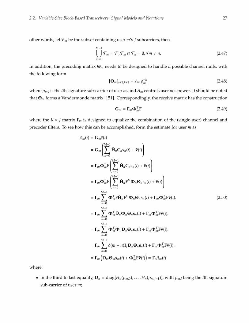
2.2. Variable-Size Block-Based Transceivers: Signal Models and Notations 27
other words, let Fm be the subset containing user m’s J subcarriers, then
M−1⋃
m=0
Fm = F ,Fm ∩ Fn = ∅,∀m , n. (2.47)
In addition, the precoding matrix Θm needs to be designed to handle L possible channel nulls, with
the following form
[Θm]l+1,k+1 = Amρ−km,l (2.48)
where ρm,l is the lth signature sub-carrier of user m, and Am controls user m’s power. It should be noted
that Θm forms a Vandermonde matrix [151]. Correspondingly, the receive matrix has the construction
Gm = ΓmΦTmF (2.49)
where the K × J matrix Γm is designed to equalize the combination of the (single-user) channel and
precoder filters. To see how this can be accomplished, form the estimate for user m as
sm(i) = Gmr(i)
= Gm
M−1∑
n=0
HnCnsn(i) + v(i)
= ΓmΦTmF
M−1∑
n=0
HnCnsn(i) + v(i)
= ΓmΦTmF
M−1∑
n=0
HnFHΦnΘnsn(i) + v(i)
= Γm
M−1∑
n=0
ΦTmFHnFHΦnΘnsn(i) + ΓmΦT
mFv(i).
= Γm
M−1∑
n=0
ΦTmDnΦnΘnsn(i) + ΓmΦT
mFv(i).
= Γm
M−1∑
n=0
ΦTmΦnDnΘnsn(i) + ΓmΦT
mFv(i).
= Γm
M−1∑
n=0
δ(m − n)IJDnΘnsn(i) + ΓmΦTmFv(i).
= Γm(DmΘmsm(i) + ΦT
mFv(i))
= Γmrm(i)
(2.50)
where:
• in the third to last equality, Dn = diag[Hn(ρm,0), . . . ,Hn(ρm,J−1)], with ρm,l being the lth signature
sub-carrier of user m;

2.2. Variable-Size Block-Based Transceivers: Signal Models and Notations 28
• in the second to last equality, the non-overlapping construction in (2.47) results in mutually
orthogonal selector matrices: ΦTmΦn = δ(m − n)IJ;
• in the last equality, regardless of the channel conditions encountered, GMC-CDMA results by
construction in a MUI-free output rm(i), with
rm(i) = DmΘmsm(i) + ΦTmFv(i). (2.51)
Furthermore, due to the mutual orthogonality of the selector matrix and the orthonormality of the
FFT matrix, the overall noise term ΦTmFv(i) is also white and uncorrelated for different m. As such, if
the noise term v(i) is also Gaussian, a single-user optimal detector following the MUI elimination step
will also be optimal in the multi-access scenario. In particular, the objective of the equalizer term Γm
can be achieved, in a zero-forcing manner, by setting:
Γm = (DmΘm)†. (2.52)
These results show that the GMC-CDMA design makes it possible to utilize single-user equalization
strategies for multi-access situations in an optimal manner, since it effective turns the multi-access
channel into independent parallel single-user channels [151].
2.2.4 Time-Variant Block Processing
As previously mentioned, in cases where the mobile velocity is significant enough to cause fast fading,
a BEM channel is a good alternative which makes it possible to still utilize a block processing paradigm.
It is also worthwhile to remark that, in the literature, the BEM approach has been mostly limited to
a single-user channel. This is due to the fact that the BEM channel matrix is neither diagonalizable,
nor equivalently diagonalizable by time-aliasing in a channel-independent manner [10]. An extension
using the BEM channel formulation for the multi-access case was proposed in [87]. However, besides
the increase in complexity, this extension also requires significant modifications to the underlying
transmission protocol, such that its value in practical systems is somewhat uncertain. Therefore, in
this thesis, only the single-user BEM case will be considered [23].
The block structure in this case is also similar to that depicted in Figure. 2.3; the zero-padding
scheme will be assumed. However, in this case, the quasi-static quantities are the basis coefficients
instead of the channel coefficients themselves. Using similar notations as in [10,94], a block-structured
signal model is obtained in the following. Collecting input and output in blocks of N × 1 symbols,
then for the kth block, the input block is
x(k) = [x(kN), x(kN + 1), . . . , x(kN + N − 1)]T, (2.53)

2.2. Variable-Size Block-Based Transceivers: Signal Models and Notations 29
with received block,
r(k) = [r(kN), r(kN + 1), . . . , r(kN + N − 1)]T. (2.54)
Since the channel matrix in this case is not diagonalizable, no attempt will be made to explicitly account
for possible pre-coding as in Figure 2.4.
Corresponding to (2.17), the input-output relationship is expressed as
r(k) = H(k) x(k) + v(k) (2.55)
where H(k) is a lower triangular N ×N matrix with elements
[H(k)]m,n = h(kN + m − 1; m − n). (2.56)
Due to zero-padding, so that the last L (channel length) elements of x(k) are zeros, IBI is prevented.
The channel matrix is expressed in terms of the basis functions as
H(k) =
Q∑
q=0
DqHq(k) (2.57)
where
Dq = diag[1, e jwq , . . . , e jwq(N−1)] (2.58)
and Hq(k) is an equivalent channel matrix with elements constructed from the basis coefficients hq,l(n)
in (2.18).
Next, due to slow variations, the coefficients hq,l(n) are block-invariant, i.e.,
hq,l(n) , hq,l(k), n = kN, . . . , (k + 1)N − 1 (2.59)
are constants for the kth block (recall that n is the discrete-time index, while k is the block index).
Then, the equivalent N × N channel matrix Hq(k) is Toeplitz, with the first column constructed from
[hq,0(k), hq,1(k), . . . , hq,L(k)]T.
Hence, the equivalent block matrix Hq(k) is composed entirely of time-invariant (with respect to
the same block) quantities, with a Toeplitz structure. In other words, the time-variance exhibited
by the channel matrix H(k) is now captured by the basis functions in Dq. This reduction facilitates
the estimation of the block-invariant coefficients [hq,0(k), hq,1(k), . . . , hq,L(k)], which can then be used to
reconstruct H(k) in (2.57). In Sec. 2.3.3, methods for estimating the channel will be presented.
Once the channel is known or estimated, an MMSE block linear equalizer (BLE) is obtained as
follows for the kth block [10],
GMMSE(k) =
(H(k)HH(k) +
σ2v
σ2x
IN
)−1
H(k)H (2.60)

2.3. Channel Identification for Variable-Size Block Systems 30
where IN is the N × N identity matrix, σ2v and σ2
x are respectively, the noise and symbol variances in
(2.17). Note that the high complexity associated with inverting (potentially large) matrices in (2.60)
can be alleviated, at the expense of reduced equalization quality, by utilizing a time-varying FIR
equalizer [10].
2.3 Channel Identification for Variable-Size Block Systems
2.3.1 Contributions
In the previous section, methods for block processing and channel equalization for a variable-size block
system have been proposed with the assumption that a priori knowledge of the channel is available.
In practice, the channel needs to be estimated. Therefore, the contribution of this section is to derive
corresponding channel identification approaches in the context of a variable-size block framework.
Both the time-invariant and time-variant cases are considered respectively in Sec. 2.3.2 and Sec. 2.3.3.
Remark: Applicability of the Variable-Size Block Approach and Other Channel Identification
Methods
It should be remarked that the identification methods presented in this section have been deliberately
kept simple, being essentially the classical maximum likelihood (ML) estimators. Indeed, the estab-
lished literature on channel identification offers myriad alternatives, some with drastic performance
advantages. However, it is crucial to realize that the goal of the proposed variable-size block method-
ology is not to supplant other channel estimators. Instead, the perspective here is to start from an
existing channel identification method, and consider what improvement can be made. Specifically, the
variable-size block approach focuses on the channel changes to improve upon the potential amount
of training available to these estimators. In other words, the same kind of improvement can be reaped
using a different block channel estimator. With a variable-size block, there is a potential to gather more
available training so that a more accurate estimate is obtained (using the same algorithm). Of course,
the degree of improvement would depend on the specific class of estimators used, e.g., using an ML
estimator vs. a more modern estimator.
Therefore, the rationale for focusing on a simple estimator in this section is twofold. First, it shows
that complicated estimators are not needed to practically utilize a variable-size block approach. Second,
the baseline performance with a simpler estimator illustrates more directly, without other extraneous
distractions, the kind of relative gain that can be expected. Certainly, improved performance is
expected with a more modern estimator. For example, a subspace-based semi-blind estimator can be

2.3. Channel Identification for Variable-Size Block Systems 31
used to achieve a higher performance improvement with the variable-size block approach [22].
2.3.2 Channel Identification for Time-Invariant Block Processing
In the time-invariant block processing scheme, the channel h[n] can be estimated using a maximum
likelihood estimator, with training symbols. This is ultimately where the variable-size block advantage
is realized: a larger accumulated block provides more training and thus better channel estimate.
Consider the first fundamental block in an accumulated block, with M consecutive training symbols
located by the index set I1 = {k, . . . , k+M−1}, i.e., x[k], . . . , x[k+M−1] are known symbols. The received
signal is
rI1 = xI1 h + vI1 (2.61)
where
rI1 = [r[k + L − 1], . . . , r[k + M − 1]]T, (2.62)
vI1 = [v[k + L − 1], . . . , v[k + M − 1]]T, (2.63)
h = [h[0], . . . , h[L − 1]]T, (2.64)
and,
xI1 =
x[k + L − 1] · · · x[k]...
...
x[k + M − 1] · · · x[k + M − L + 1]
. (2.65)
Note that when pre-amble training and zero-padding guard intervals are used (see Fig. 3.3), then
the dimensions of the above quantities can be enlarged for better estimation. If x[k− L + 1], . . . , x[k− 1]
correspond to the guard symbols and are thus known to be all equal to zero, then the received signal
can be formed as rI1 = [r[k], . . . , r[k + M− 1]]T, with appropriate modifications of the related quantities
from (2.61).
Similarly, the second fundamental block has training symbols with the index set I2 = B⊕ I1, where
⊕ denotes element-wise addition with a scalar B, which is the number of symbols in a fundamental
block. Then,
rI2 = xI2 h + vI2 . (2.66)
Thus, if there are µ fundamental blocks in the accumulated block,
rI1
. . .
rIµ
=
xI1
. . .
rIµ
h +
vI1
. . .
vIµ
(2.67)

2.3. Channel Identification for Variable-Size Block Systems 32
or
rΣ = xΣ h + vΣ. (2.68)
The ML channel estimate is then
hML = x†ΣrΣ (2.69)
where (·)† denotes the Moore-Penrose pseudo-inverse [62].
2.3.3 Channel Identification for Time-Variant Block Processing
Training symbols are also used to identify the channel for the BEM scenario. First the single-block
identification will be presented, followed by the multiple-block extension.
Single-Block Identification
From (2.17), to determine an output symbol r(n), the input symbols x(n − L), . . . , x(n) are needed.
However, if T training symbols in the kth block, xT(k) = {x(n), n = kN, . . . , kN + T − 1}, are located in
the pre-amble position (at the beginning of the block), then, due to zero-padding in the input blocks, the
corresponding first T output symbols rT(k) = {r(n), n = kN, . . . , kN + T − 1} can be determined. Hence,
rT(k) =
Q∑
q=0
Dq,T Hq,T(k) xT(k) + vT(k) (2.70)
where Dq,T, Hq,T(k), vT(k), are sub-matrices of the matrices in (2.17), (2.57), partitioned from the upper-
left corner in obvious manners, e.g.,
Dq,T = diag[1, e jwq , . . . , e jwq(T−1)] (2.71)
is a T×T diagonal (sub)matrix of Dq. Extensions to the more general cases where the T training symbols
are not located in pre-amble, e.g., dispersed throughout the block, require relatively straightforward
notational modifications, and can be found in [94].
For T > L, the Toeplitz structure of Hq,T(k) implies that
Hq,T(k) xT(k) = XT(k) hq(k), (2.72)
where XT(k) is a T × (L + 1) Toeplitz matrix, with the first column consisting of the training symbols
[x(0), . . . , x(T − 1)]T and
hq(k) = [hq,0(k), hq,1(k), . . . , hq,L(k)]T (2.73)

2.3. Channel Identification for Variable-Size Block Systems 33
which is the block-invariant coefficients from (2.59). Then, from (2.70), (2.72),
rT(k) = Φ(k) h(k) + vT(k) (2.74)
where h(k) = [h0(k)T,h1(k)T, . . . ,hQ(k)T]T is the (block-invariant) vector of all the basis coefficients, and
Φ(k) the matrix of (modulated) training symbols defined as:
Φ(k) =[D0,T XT(k),D1,T XT(k), . . . ,DQ,T XT(k)
], (2.75)
with Dq,T being the diagonal matrices of basis functions from (2.70). Then a maximum-likelihood
estimate of h(k) can be obtained as
hML(k) = Φ(k)† y(k) (2.76)
where (·)† denotes the Moore-Penrose pseudo-inverse as before.
Multiple-Block Identification
When the basis coefficients h(k) remain valid over M multiple consecutive blocks, each of N data
symbols (see Sec. 3.2), the training symbols from these multiple consecutive blocks can be combined
for improved channel identification as follows [23].
Consider the next consecutive block k + 1. Similar to (2.74),
rT(k + 1) = ΦMB(k + 1) h(k) + vT(k + 1) (2.77)
where the fact that h(k + 1) = h(k) is used.
Furthermore, the multiple-block matrix, ΦMB(k + 1), of modulated training symbols for the first
consecutive block is related to the single-block version by
ΦMB(k + 1) = e jNwqΦ(k + 1). (2.78)
And more generally,
ΦMB(k + κ) = e jκNwqΦ(k + κ). (2.79)
This can be seen by computing (2.18) for the κth consecutive block:
h(n + κN; l) =
Q∑
q=0
hq,l(n + κN)e jwq(n+κN) =
Q∑
q=0
e jκNwq(hq,l(n)e jwqn), (2.80)
which accordingly changes Dq in (2.57) to the diagonal matrix e jκNwqDq.

2.4. Summary 34
As a result, the M consecutive blocks combine to yield
rT(k)
rT(k + 1)...
rT(k + M − 1)
=
ΦMB(k)
ΦMB(k + 1)...
ΦMB(k + M − 1)
h(k) + vΣ(M) (2.81)
or
rΣ(M) = ΦΣ(M) h(k) + vΣ(M). (2.82)
Then a maximum-likelihood estimate of h(k) can be obtained as
hML(k) = ΦΣ(M)† rΣ(M) (2.83)
Evidently, a larger M provides a more accurate estimate of the overall basis coefficients h(k), since
more training symbols are available.
2.4 Summary
In this chapter, various issues regarding the system modeling aspect are addressed. First, statistical
characterizations of the mobile channel provide useful ways to classify a particular channel as either
slow vs. fast fading, or frequency flat vs. frequency selective. Then, block processing methods are
proposed for efficiency. In particular, a variable-size block method is introduced to take full advantage
of the available training whenever the channel is in a quasi-static state. Once the channel models
have been described, corresponding equalization and estimation methods are presented. A crucial
assumption has been made in this chapter, that the accumulated block exists over a quasi-static time
duration of the channel. In the following chapter, specific algorithms for ensuring this validity will
be presented. In addition, other adaptation methods will be proposed, all with the system models
established in this chapter as the foundation.

Chapter 3
Adaptation Methods for QoS Regulation
The ability to regulate the quality of service (QoS) in a communication network is an important and
practical goal, especially in a resource sensitive scenario. In the literature, myriad methods have
been proposed to deliver QoS improvements, from just about any layer or level of the network
[5,15,32,35,51,52,67,73,82,83,110,114,121,155]. Therefore, it would be beyond the scope of this thesis
to merely survey all these existing techniques even in a superficial manner. Instead, the goal of this
chapter is to examine specific schemes that are particularly suitable for subsequent integration in a
unified framework. Among other properties, the methods should exhibit flexibility and adaptivity,
which should be parametrically adjustable, so that they can accommodate a wide range of operating
conditions. Moreover, the proposed techniques have been originally designed or specifically modified
from existing work to complement the system models developed in the previous chapter.
As such, this chapter cannot be regarded as an exhaustive repository of currently available tech-
niques, but rather should be considered as an initial foundation or placeholder for supplementary or
future work. In other words, for applications that require or can provide additional adaptation capa-
bilities [5], they can be considered in an analogous fashion, with similar design factors and constraints.
To recall, this thesis advocates the following design paradigm, with three intimately related classes
of methods: modeling, adaptation and integration. In this context, this chapter examines the second
category, which is substantiated with original work done in this area.
It should be noted that, for most of the chapter, the proposed algorithms do not explicitly consider
multi-access or multi-user scenarios. Recalling from the previous Chapter 2: a unique feature of
the GMC-CDMA scheme is that, assuming this multi-carrier scheme can implemented, estimation
and equalization techniques proposed in a single-user setting will also be directly applicable in a
multi-user situation. This is because the GMC-CDMA scheme makes it possible to eliminate MUI
regardless of the channel encountered, as long as the ISI extent as defined by the channel length is
known to a sufficient degree (in particular, a good upperbound should be available), and also the
35

3.1. Quality of Service (QoS) Metrics: A Brief Survey 36
frequency spectrum should be large enough to accommodate the total number of users according
to the sub-carrier requirements (for reliable pre-coding). However, in Sec. 3.5, a multi-user setting
with multiple antennas will be explicitly considered. The purpose is two-fold: (1) to demonstrate the
potentials of spatio-temporal processing using multiple antennas for multi-access communications; (2)
to show that enhancing the proposed framework with additional requirements, e.g., multiple antennas
and users, involves mostly straightforward—albeit somewhat meticulous—notational changes in the
signal model. In other words, the proposed framework is highly flexible and conducive to future
developments.
3.1 Quality of Service (QoS) Metrics: A Brief Survey
Quality of service is a rather loaded or polysemous term, in that depending on the context considered,
many criteria may be construed as conveying system quality [2,5,57,100,125]. Therefore, recalling that
the motivation for considering QoS is to attain a unified method for assessing system performance, the
following properties are essential: relevance, consistency, repeatability and numerical quantifiability.
From a signal processing perspective, the last point is perhaps most practical, because without a
numerical value, decision algorithms may not be feasibly proposed. At the same time, if the numerical
values do not reflect in a relevant manner the intended performance, the signal processing method
applied cannot be expected to fulfill the intended objective. In a communication network, the following
criteria may be sensibly considered as indicators of the QoS [131, 155]:
• Data rate: the rate of information that is transferred over a network. Depending on the nature
of the data, the rate required can vary significantly. For example, a text message needs only low
data rate, while a video stream may consume a significant amount of information over time.
• Bit-error rate (BER), mean-squared error (MSE) [62, 63]: metrics to quantify the errors between
the transmitted and received signals. These quantities are arguably among the most commonly
used metrics to compare system performances.
• Latency: the delay imposed by the communication system. Some applications may be more
delay-sensitive or delay-tolerant than others, e.g., a real-time conversation is often delay-
sensitive.
• Security: even though it certainly represents an important system feature, treating security as a
QoS parameter to be assigned has not been a very popular practice until more recently [52,100].
The reason is that many definitions of security exist, and metrics for security are also difficult to

3.1. Quality of Service (QoS) Metrics: A Brief Survey 37
be constructed. However, when a reliable encryption scheme is used, the system security can be
characterized almost exclusively based on the cryptographic key length involved [98, 135].
• Economic costs or profits: the viability of a proposed system often depends on its potential to
generate economic incentives. In some cases, this may be reflected by the number of network
subscribers. However, other short-term and long-term scenarios may distort the obtained results
in an unpredictable manner. For example, while the initial number of subscribers may indicate
economic prosperity, if the social and political changes somehow discourage users from adopting
a certain communication application, then significant measures beyond the signal processing
may be needed to ensure a timely and adequate response.
While the above criteria can be used to propose QoS methods, practical signal processing algorithms
often do not directly account for or make decisions based on these criteria. This is due either to
mathematical intractability in the problem formulation, or more practically to difficulty in obtaining
these quantities in an accurate or timely manner. For example, estimating the BER accurately and
on a regular basis may require modified communication protocol or unnecessarily high resource
consumption [5, 102, 152].
Instead, a variety of QoS metrics are typically used to enable system adaptation. These metrics
are more readily available quantities, that are nonetheless related to the QoS in a meaningful manner.
Specifically, the relationship between a QoS criterion and an associated QoS metric should ideally be
bijective (one-to-one and onto) and monotonic. Then, a proposed signal processing method may be
based entirely on the QoS metric, and still deliver adequate QoS performance. However, since ideal
QoS metrics may not always be found, the following cases and practical issues need to be considered.
• A QoS metric may be ideal in an existential sense only. For instance, in general, it is known
that BER is a monotonic and bijective function of the channel SNR. However, for certain types
of channel settings, the relationship may be highly non-linear or may not even admit a closed
form expression. In other words, while the ideal relationship certain exists, it may not be known
or expressible in a practical form. Then, the adaptation method needs to rely on empirical or
simulated performance to parametrically set the thresholds for system performance.
• A QoS metric may be bijective but non-monotonic. It is still possible to propose adaptation
methods based on this metric. However, the system performance is prone to metric errors:
minor errors may translate to high performance errors. Moreover, the system adaptation may
not be possible based on a threshold-scheme, but may have to be based on a table of values,
which should moreover be sufficiently exhaustive.

3.2. Channel Tracking and Block-Size Adaptation 38
• A QoS metric may be injective (one-to-one) but not surjective (onto). This implies that certain
QoS performance values may not be monitored or assessed by the metric. However, in this case,
such a scenario likely indicates that the requested QoS performance is infeasible with the given
hardware resources or infrastructure (i.e., the set of feasible solutions is empty, in the context of
Chapter 5).
• A QoS metric may be surjective but not injective. Since ambiguous cases exist, with potential
large differences in input values, the system performance may also be prone to metric errors.
Moreover, a threshold-based scheme may not be possible.
It should be noted that the last case is perhaps the least desirable. This is because without an injective
mapping, the relationship needs to be known exhaustively to ensure that all cases are accounted for.
Otherwise, the system performance may vary unpredictably whenever the metric deviates from a
known or nominal range of values.
Various quantities have been used as QoS metrics to adapt the system structure and improve the
QoS performance, including training or pilot data symbols, equalizer outputs, or estimated errors
from decision-directed algorithms [52, 84]. Generally, for methods that target the BER performance,
the metric is usually related to the signal-to-noise or signal-to-interference ratios. And for methods
that seek to improve the data rate, the transmission protocol or data block structure usually provide
the suitable metric for adaptation. Moreover, applications of techniques not originally intended for
resource allocation can also be exploited as novel QoS metrics. For example, introduced for security
and authentication purposes, watermarks have been reported to convey the QoS in a promising
manner [29, 50].
3.2 Channel Tracking and Block-Size Adaptation
3.2.1 Motivations and Previous Works
Achieving high spectral efficiency is an important goal in communication. However, it is equally
important that the QoS, quantified by the BER, does not deteriorate as result of this goal. In this
section, channel tracking methods that allow for block-size adaptation are proposed. Such approaches
allocate training resources for improving the spectral efficiency, while maintaining good QoS in the
block-by-block communication systems described in Chapter. 2.
With the advent of systems employing high-frequency carriers and used in high-speed environ-
ments, the quasi-static channel assumption is becoming more questionable. Essentially, the channel
can be regarded as constant over a block if the block duration is less than the channel coherence time

3.2. Channel Tracking and Block-Size Adaptation 39
TC. However, the channel coherence time is itself actually a statistical measure, whose precise formula
depends on the definition criterion. Loosely speaking, [122, 136]
TC ≈ 1fm
(3.1)
or alternatively, defined as the time over which the time correlation function is above 0.5 [122, 136]
TC ≈ 916π fm
(3.2)
where fm is the maximum Doppler shift given by
fm =vm
λ=
vm fcc
(3.3)
with vm being the mobile speed, λ the wavelength, fc the carrier frequency and c the speed of light.
The relationship with the block duration can also be viewed using the normalized Doppler shift fmTS,
where TS is the symbol duration. Then, using (3.1), a block is within a coherence time if the number
of symbols in the block, i.e. the block size BS, is
BS <1
fmTS. (3.4)
Regardless of which definition, (3.1) or (3.2), is used, the coherence time TC is inversely proportional
to both the carrier frequency fc and the mobile speed vm. Hence, with an increase of the carrier
frequency fc in modern systems, TC tends to become shorter. In practice, the block duration is
chosen to be significantly less than TC in order to justify the quasi-static assumption. For example, in
GSM [122, 136], a block duration is 0.577 ms, while TC ≈ 11 ms (using (3.1) with fc = 960MHz, v = 100
km/h).
With an increased carrier frequency, e.g. fc < 3.5 GHz in the developing IEEE802.20 standard, the
coherence time reduces to TC ≈ 3.6 ms. And with target bitrates on the order of 1 Mbps, the symbol
duration TS ≈ 2µs (assuming 2 bits/symbol, e.g. using 4-QAM [60, 136]). Hence, the normalized
Doppler shift is fmTS ≈ 5.55 × 10⁻⁴, and a coherence time contains at a maximum 1/( fmTS) = 1800
symbols.
For visualization purposes, Fig. 3.1 shows typical fading envelopes versus the symbol index for
the above calculated normalized Doppler shift fmTs ≈ 5.55 × 10⁻⁴, and also for fmTs ≈ 5.55 × 10⁻⁵.
Here, the time variations are described by the Jakes power spectral density (see (2.14)). The smaller
normalized Doppler shift corresponds to a more slowly varying channel.
In coping with the reduced coherence time TC, a number of approaches can be considered. First,
the channel invariance assumption can be eliminated, and new receiver structures can be designed.

3.2. Channel Tracking and Block-Size Adaptation 40
0 1 2 3 4 5 6 7 8
x 104
−40
−30
−20
−10
0
10
20
Data symbol
Rec
eive
d en
velo
pe (
dB)
(a)
0 1 2 3 4 5 6 7 8
x 104
−60
−40
−20
0
20
Data symbol
Rec
eive
d en
velo
pe (
dB)
(b)
Figure 3.1: Received envelopes over fading channels at carrier frequency fc = 3.5 GHz: (a) Mobile
speed vm=100 km/h, or normalized maximum Doppler shift fmTS = 5.55 × 10⁻⁴; (b) vm=10 km/h, or
fmTS = 5.55 × 10⁻⁵.
However, suppose that such changes are not permissible, e.g. due to existing infrastructure or hard-
ware constraints. Then, the question is whether basic block-by-block techniques can still be used in
rapidly time-varying channels. We examine techniques for achieving reliable communications in such
channels, while still using the same basic block-by-block receiver methodology.
Ultimately the goal is to shorten the block duration in some manner, so that it remains within the
coherence duration. Following are example methods that can be considered:
• (S1) Reduce the number of data symbols per block:
To reduce the overall block duration, the symbol duration TS must not be increased. With this
solution, the transmission efficiency, i.e., the ratio of useful data symbols over all symbols in a
block, can be severely affected, especially in rapidly varying channels.
• (S2) Reduce the block duration:
Alternatively, the same number of symbols in a block can be maintained, but the symbol duration
TS is reduced. While the transmission efficiency is maintained, if the symbol duration is too short

3.2. Channel Tracking and Block-Size Adaptation 41
relatively to the channel delay spread, the channel becomes highly frequency-selective, with
severe intersymbol interference (ISI). The use of a high-complexity equalizer would be needed
for acceptable QoS.
• (S3) Use a variable-size block approach:
A key bottleneck in the previous two methods is the assumption of a fixed-size block, chosen
to satisfy the worst case scenario. This is inefficient when the encountered channel is slowly
changing, e.g. when the mobile speed is low. To this end, several relationships between the block
size, training size, channel conditions and relevant issues are discussed in [36,104,146,161]. The
relevant conclusion is that to achieve a prescribed levels of performance, the amount of training
and the block size should be selected according to the channel conditions. However, no attempt
is made in these works to adaptively change the block size based on the operating channel
encountered. However, a packet size adaptation problem can be found for ARQ protocols
in [103], where the packet size is adapted based on estimates of bit-error-rate. Therefore, the
idea of a variable-size block [22] is to use a shorter block when the channel is changing quickly.
Conversely, durations over which the channel is slowly changing will be exploited to use a
larger block. As will be seen, this enables a better use of the available training symbols for
improved transmission efficiency and QoS. Moreover this construction can be achieved entirely
at the receiver.
Remark: Variable-Size Block Construction and Process Segmentation
The variable-size block construction can also be realized by using a process segmentation approach.
In the process segmentation literature, data sequences are segmented into locally stationary groups
for recognition and monitoring [11, 85, 107]. Indeed, based on analysis of variance (ANOVA) and
minimum description length (MDL), variable-size blocks can be constructed to produce improved
equalization performance [22]. However, the aim of this thesis is to utilize channel tracking not
merely as a tool for block-size adaptation [24]. Instead, as will be seen in the remainder of this chapter,
it serves as the common front-end for other adaptation methods, as well as for the optimization
framework in Chapter 5, which all depend in some manner on the operating channel conditions. As
such, the process segmentation approach is not considered in this thesis.
3.2.2 Contributions
In this section, a variable-size block construction approach based on channel tracking is proposed.
Essentially, within a multi-state channel model established in the previous chapter, the goal is to track

3.2. Channel Tracking and Block-Size Adaptation 42
scenarios where the same channel state is maintained over consecutive time durations to construct a
larger-size block. To reap the advantage of this scheme, a corresponding block structure is needed.
Therefore, the contribution is made first in designing a variable-size block as an aggregate of smaller
fundamental blocks, in Sec. 3.2.3. The advantage of this scheme is that it can be performed entirely at
the receiver, and without requiring changes to the underlying infrastructure used for a fixed-size block
scheme. Subsequently, in Sec. 3.2.4, a threshold-based channel tracking method is proposed using the
associated equalization error.
3.2.3 Variable-Size Block Structure
A variable-size block structure, based on a conventional fixed-size block, is described in this section.
The idea is to approximate the channel as constant or quasi-static over some interval, which should be
less than the coherence time. In the context of a time-varying mobile channel, Fig. 3.2 illustrates this
approximation on a channel with normalized Doppler shift fmTS = 1×10⁻³ for two different fixed-size
blocks: (a) a smaller block of 100 data symbols; and (b) a larger block of 400 data symbols. According
0 400 800 1200 1600 2000 24002400−40
−30
−20
−10
0
10
20
Data symbol
Rec
eive
d en
velo
pe (
dB)
(a) Quasi−static approximation (Burst size = 100 symbols)
0 400 800 1200 1600 2000 24002400−40
−30
−20
−10
0
10
Data symbol
Rec
eive
d en
velo
pe (
dB)
(b) Quasi−static approximation (Burst size = 400 symbols)
Figure 3.2: Quasi-static Channel Approximation for fmTS = 1× 10⁻³ using: (a) Fixed-size blocks of 100
symbols; (b) Fixed-size blocks of 400 symbols.

3.2. Channel Tracking and Block-Size Adaptation 43
to (3.4), the block size chosen in this case should be less than 1000 symbols (i.e., approximately within
a coherence time interval of this relatively fast-fading channel). However, as can be seen from the
quasi-static approximations and the above discussions, this guideline does not necessarily result in
appropriate block sizes. Indeed, for this scenario, the smaller block approximates the channel more
accurately; but a total of 24 fixed data blocks would be needed. The larger block approximates the
same channel using fewer data blocks, with a total of 6 in this case. With a fixed overhead of training
symbols per block, it is more desirable to use the larger block, since the transmission efficiency (which
is proportional to the spectral efficiency) would be higher. However, as illustrated by Fig. 3.2 (b), the
larger block approximation is quite inaccurate at certain times, e.g., the deep fade around symbol 1000
is missed entirely. On the other hand, the smaller block is rather redundant at certain times, e.g. over
the symbol range 1200-1500, a single-block approximation suffices. Hence, a compromise between the
two different block sizes, using a variable-size block, is advantageous in terms of efficiency.
Fig. 3.3 shows a potential variable-size block structure. The key idea here is to realize the distinction
between a transmitted and a received block: regardless of what the transmitter sends, the receiver
ultimately can make a choice on what it considers a received block (used for further processing, such
as channel estimation). Then, the transmitter simply transmits fixed-size fundamental blocks. At the
receiver, a variable-size block is constructed by combining consecutive transmitted fundamental blocks
appropriately. For this scheme to function, as in a fixed-size block system, the fundamental blocks
need to satisfy the quasi-static channel conditions. The difference is that, by tracking the channel, the
receiver can detect a slowly changing duration, and accordingly adapts the block size by combining
the consecutive fundamental blocks within this duration. The result is a larger accumulated block,
composed of fundamental blocks, with an enlarged set of training symbols delivering a more accurate
channel estimation.
• Conceptual Variable-Size Block Construction with Prior Channel Knowledge
To illustrate the described procedure, Fig. 3.3(a) shows an example scenario, where the channels
for eight consecutive fundamental blocks are known a priori, and designated as G1,G2, ...,G8.
A fixed-size block receiver simply assumes that these channels are all different, and constructs
received blocks of the same size as the transmitted blocks as shown in Fig. 3.3(b). However, if
the underlying channels are not all different, then a variable-size block can combine appropriate
consecutive fundamental blocks to form larger accumulated blocks, while still satisfying the
quasi-static assumption. For example, if G2 = G3, G4 = G5 = G6, G7 = G8, then the unique chan-
nels can be re-designated as H1,H2,H3,H4, from which there would be four enlarged variable-size
accumulated blocks as in Fig. 3.3(c).

3.2. Channel Tracking and Block-Size Adaptation 44
Figure 3.3: Variable-size block structure with pre-amble training symbols: (a) Quasi-static channel
approximations for each block, where some channels may be the same, e.g. G2 = G3 ≡ H2; (b) Fixed-
size block processing, assuming all channels are different; (c) Variable-size (received) block processing,
exploiting knowledge of channel similarities.
Evidently, this construction is merely a conceptual one, since it requires prior channel knowledge.
In Sec. 3.2.4, a practical construction scheme is proposed to address this limitation.
• Remark
In considering the implications of the preceding example construction, it is useful to refer to
Fig. 3.2(a). It shows examples of cases where channels from consecutive blocks may be regarded
as equal. For instance, in the quasi-static approximation using a block size of 100 symbols, the
channels associated with the consecutive blocks between the symbols 1200-1499 are essentially
equal. This may correspond to the scenario in Fig. 3.3 where three consecutive channels are equal:
G4 = G5 = G6. Then, a longer accumulated block may be used over these three blocks (in fact,
over four consecutive blocks between symbols 1200-1599, as shown in Fig. 3.2(b)). Furthermore,
the longer accumulated block would have more total training symbols available for improved

3.2. Channel Tracking and Block-Size Adaptation 45
estimation and equalization performance, as explained previously in Sec. 2.2.3.
• Comparisons to a Fixed-Size Block Structure
From a transmitter perspective, there is essentially no difference in terms of the block structure.
The fundamental block size is still specified by the highest-speed fm. However, in rapidly time-
varying channels, the variable-size block structure is more attractive, because it has the potential
to maintain good spectral efficiency.
Indeed, consider using solution (S1), from Sec. 3.2.2, to reduce the number of data symbols per
block. Then, to maintain the same transmission efficiency, the number of training symbols must
also be reduced. However, estimation and equalization depends on the raw number of training
symbols (and not the transmission efficiency). Hence, a fixed-size block, which in general
has insufficient training symbols in rapidly time-varying channels, will suffer from significant
performance degradation due to unsuccessful channel estimation and equalization. By contrast,
a variable-size block has the potential to regain the performance loss by making the best use of
the available training symbols.
The effect of training symbol assignment or placement is not investigated here. While optimal
training placement can have a significant impact on the overall performance [37], this work has
a different perspective: given a training regime (e.g. pre-amble, mid-amble, or superimposed),
the problem is how to combine the available training symbols from different blocks in an ad-
vantageous manner, notably by tracking the channel. This is based on the assumption that more
training symbols would yield better overall performance.
3.2.4 Channel Tracking for Variable-Size Block Construction
Utilizing the quasi-static estimation and equalization methods previously described in Section 2.3, a
threshold-based scheme for detecting channel changes is proposed in this section. The QoS metric
in this case is the estimation error. The transmission efficiency or the data rate is the QoS perfor-
mance being improved. Indeed, as variable-size block construction enables training reduction, while
maintaining the same BER performance, more data symbols can be transmitted instead of redundant
training information. As such, a receiver algorithm for processing variable-size blocks is also presented
to illustrate the procedure.

3.2. Channel Tracking and Block-Size Adaptation 46
Threshold-Based Change Detection
The variable-size block construction problem can be stated iteratively. Suppose that, at the current
iteration, the accumulated block Bcurrent is composed of µ consecutive fundamental blocks, Bcurrent =
{bk, . . . , bk+µ−1}, and that the channel is the same over the entire Bcurrent. Then, upon the reception of
the candidate fundamental block bk+µ, the choices are:
(H1) Add bk+µ to the current accumulated block, forming Bpotential = {bk, . . . , bk+µ}. Continue with
bk+µ+1 as the next candidate.
(H2) Reject bk+µ, terminate Bcurrent and accept it as the best choice. Re-initialize with bk+µ as the start
of a new accumulated block.
To decide whether to accept (H1) or (H2), the following procedure is performed:
1. In (2.69), estimate the channel using Bcurrent, returning an estimate hC.
2. Similarly, estimate the channel using Bpotential, returning an estimate hP.
3. Compute the squared norm of the estimation difference:
ρed = |hC − hP|2. (3.5)
4. Compare to a threshold ρth for detection decision:
ρed − ρth
H2
RH1
0. (3.6)
In the above, ρed is a second-order measure of the channel change in the following sense. Suppose that
the underlying channel of Bcurrent is h, and that hC is a close estimate of the true channel. Then if bk+µ
experiences the same h, the resulting estimation difference
hed = hC − hP (3.7)
is small. But if the channel has changed for the candidate bk+µ, the estimation difference hed is large.
In (3.5), a squared norm is used to quantify this difference. The utility of this choice is made evident
by examining (3.13) and (3.14), as explained next.

3.2. Channel Tracking and Block-Size Adaptation 47
Threshold Function Selection
Let the true channel be h, then depending on the detection decision (H1) or (H2), the channel estimation
error hce is either
hce,C = h − hC (3.8)
or
hce,P = h − hP. (3.9)
The channel estimation error is unknown, since the true h is not available. However, an upperbound
for its squared norm can be approximated as follows. Noting that
|hed|2 = |hce,C − hce,P|2, (3.10)
and assuming independence of the estimation errors, so that
E(h∗ce,C hce,P) = E(hce,C h∗ce,P) = 0, (3.11)
then
E(|hed|2) ≈ E(|hce,C|2) + E(|hce,P|2) ≥ E(|hce|2) (3.12)
which means that by keeping the estimation difference hed small as in (3.6), the resulting channel
estimation error hce should also be statistically small.
Next, consider the effect of a channel estimation error, with impulse response hce[n], at the equalizer
input. Adapting the signal model (2.17) to this context,
r[n] = h[n] ? x[n] + v[n]
= (h[n] − hce[n]) ? x[n] +
v[n]︷ ︸︸ ︷hce[n] ? x[n] + v[n]
= h[n] ? x[n] + v[n] + v[n]
(3.13)
where h[n] is the estimated channel impulse response (i.e., corresponds to either hC or hP depending
on the detection decision). Hence for an equalizer using the estimated channel h[n], the second term
v[n], due to the channel estimation error, can be viewed as an additional noise source. For a particular
channel realization, this estimation noise error has variance
E(|hce[n] ? x[n]|2) = σ2x
L−1∑
l=0
|hce[l]|2 = σ2xρce (3.14)
where σ2x is the average symbol energy. From (3.13), when noise is significant (low SNR), a small
estimation error does not necessarily deliver significant performance gain. However, at high SNR,

3.3. Adaptive Modulation 48
the channel estimation error becomes the bottleneck. In fact, it is well-known that channel estimation
errors can result in an error floor at high SNR [62]. Hence, with a fixed average symbol energy σ2x,
the channel estimation error variance (3.14) should be proportional to the channel noise variance σ2v
for optimal performance tradeoff. The above implies that the optimal threshold ρth in (3.6) needs
to be a function of the noise variance. Since the primary goal is to demonstrate the performance
improvement compared to a fixed-size block in time-varying environments, the effect of threshold
optimization will not be explored. Instead, in Sec. 3.6, a sensibly predetermined threshold function
ρth, weighted against the noise variance σ2v, will be used to assess potential improvement. In addition,
an alternative formulation with respect to constrained optimization is also considered in Sec. 5.3.
Receiver Processing with a Variable-Size Block
Implicit in the tracking procedure is the requirement of a buffer for computing the intermediate hC
and hP, which introduces additional complexity and also latency. To alleviate the incurred penalties,
a maximum block size can be imposed. Fortunately, as will be illustrated in Sec. 3.6.1, even a modest
block size can yield significant performance gain. In fact, when the receiver already has sufficient
training to equalize the channel accurately, i.e. approaching the MMSE lower-bound, enlarging the
accumulated block does not produce further appreciable improvement. Also, constraining the block
size minimizes the propagation of estimation errors. At low SNR, with inaccurate channel estimates,
tracking can erroneously accumulate more fundamental blocks than possible, thus violating the quasi-
static requirement.
Accounting for the above factors, Table 3.1 describes a conceptual receiver procedure for processing
variable-size blocks.
Essentially, while the accumulated block has not exceeded the maximum size, the receiver iter-
atively considers consecutive candidate fundamental blocks for inclusion, using a threshold-based
change detection scheme.
3.3 Adaptive Modulation
3.3.1 Motivations and Previous Works
In the previous section, tracking enables constructing a variable-size block over which the channel can
be considered quasi-static. In other words, the channel quality over each such constructed block can
be considered constant, while from block to block, the channel quality changes. If the channel quality
is further known for each block, it is also possible to adapt the modulation mode for the data symbols

3.3. Adaptive Modulation 49
ρth: threshold for decision
Ntotal : total number of fundamental blocks to be processed
bsizemax: max number of fundamental blocks in an accumulated block
s: fundamental block defining the start of the current accumulated block
I. Initialization
1. Set s = 1
II. Iteration
for i = 2, 3, · · · ,Ntotal
if (i − s + 1 ≥ bsizemax) or (i == Ntotal)
1. Set the current accumulated block =
all fundamental blocks from s to i
2. Equalize the current accumulated block
3. Reset s = i + 1
else if (ρed > ρth)
1. Set the current accumulated block =
all fundamental blocks from s to i − 1
2. Equalize the current accumulated block
3. Reset s = i
Table 3.1: Variable-size block receiver with Channel tracking
on a block-by-block basis. When the channel is benign or of good quality, a higher-order modulation
constellation, e.g. 16-QAM, can be used for efficiency while still maintaining a good QoS, defined by a
target BER. However, when the channel is hostile or of poor quality, a lower-order modulation mode,
e.g. BPSK, is selected to maintain an acceptable QoS. Known as adaptive modulation [24,30,52,60,84],
this methodology permits an overall improvement in spectral efficiency. Thus, adaptive modulation
plays a key role in balancing the system integrity and efficiency in a time-varying environment.
The basic scheme of the so-called closed-loop block-by-block adaptive modulation can be summa-
rized as follows [24, 60]:
1. At the receiver, perform channel quality measurement, returning a channel metric.
2. Relate the channel metric to a suitable modulation mode, which yields the highest throughput

3.3. Adaptive Modulation 50
while maintaining the required level of QoS.
3. Signal the selected modulation mode to the transmitter to be used in the next transmission block.
It should be noted that the average transmitted symbol energy σ2x is kept the same, regardless
of the modulation mode in use. This alleviates the need of power control, which is typical for
alternative systems operating in fading channels. The QoS is nonetheless guaranteed, by using the
suitable modulation mode for an operating channel quality. In addition, the symbol rate is maintained
constant so that the required bandwidth is unchanged, regardless of the selected modulation mode.
The established literature on adaptive modulation is focused mostly on fixed-size block systems
[52,60,84]. Furthermore, most adaptive modulation schemes depend, in some manner, on the channel
knowledge. Therefore, with a fixed-size block approach, the channel estimate is limited by a fixed
number of training symbols, regardless of the operating channel. Since the estimate can be improved
with a variable-size block, the corresponding adaptation can also be more accurately achieved. In
particular, the channel quality assessment and the decision to switch the modulation mode will be
better matched with the actual channel encountered, when using a more accurate channel estimate as
provided by a variable-size block framework.
3.3.2 Contributions
In the context of QoS regulation, the use of adaptive modulation with a variable-size block is thus
explored. The first contribution in Sec. 3.3.3 involves deriving the appropriate channel metrics for the
application considered. The advantages and disadvantages of each metric, as well as the connections
between the metrics, are described. In particular, the connections between the pseudo-SNR metric
and the MSE-based metric are made [24].
Moreover, in Sec. 3.3.6, the contribution is in proposing a two-layer integration of adaptive modu-
lation and channel tracking, in order to enable improved performance in a variable-size block context.
Essentially, the additional requirement for this construction is the availability of feedback. However,
note that this same requirement is required for conventional adaptive modulation using a fixed-size
block.
3.3.3 Channel Metrics
The most appropriate metric for quantifying the channel quality in adaptive modulation is the bit-error
rate (BER). However, since the BER is often difficult to estimate directly, alternatives are often used
instead. For a frequency non-selective or flat fading channel, the short-term signal-to-noise ratio (SNR)

3.3. Adaptive Modulation 51
is an appropriate metric [30,60]. For a frequency-selective channel, the short-term SNR is inadequate,
since the influence of ISI must be taken into account. Moreover the BER performance for frequency-
selective channel is a complicated function of many factors, including channel length, power delay
profile, and even the form of equalizer used, e.g. the number taps in a linear equalizer, and the value
of the equalizer delay. In the following, we outline three possible approaches for computing a channel
metric, which can be used to guarantee a target QoS by selecting the appropriate modulation mode.
Exact Residual ISI
Given enough side information, the exact probability of error can be computed. Consider the overall
equalized channel impulse response
g[n] = f ∗[n] ? h[n] (3.15)
where f [n] and h[n] are the impulse responses of, respectively, the equalizer and the channel. Following
[24, 119], consider the equalizer output at instant n
z[n] = f ∗[n] ? r[n]
= g[δ] x[n − δ] +∑
k,δ
g[k] x[n − k] +
N−1∑
k=0
f ∗[k] v[n − k] (3.16)
where the first term is the desired signal component, the second term the residual ISI and the last term
the equalized noise. Note that g[n] is effectively an FIR filter of length N +L−1. Hence, for a particular
input sequence xJ of N + L − 1 symbols, the corresponding residual ISI term is
DJ =∑
k,δ
g[k] xJ[n − k]. (3.17)
When using M-PAM, the resulting conditional probability of error is [119]
PM(DJ) =2(M − 1)
MQ
√(g[δ] −DJ)2
σ2n
(3.18)
where σ2n is the variance of the equalized noise
σ2n = σ2
v
N−1∑
n=0
| f [n]|2. (3.19)
Hence, for a particular channel, input sequence and M, the exact probability of error can be found. A
channel metric can then be defined as
ΓISI = DJ (3.20)

3.3. Adaptive Modulation 52
and the appropriate modulation mode, i.e., the value of M, can be determined from (3.17) for a desired
QoS. Unfortunately, this exact metric is not practical, since knowledge of N + L − 1 data symbols
surrounding the desired symbol x[δ] is required (which implies knowledge of the entire sequence of
data).
Alternatively, an average and an upper-bound probability of error can be found respectively
as [119]
PM =∑
xJ
PM(DJ)P(xJ) (3.21)
and
PM(D∗J), D∗J = (M − 1)∑
k,δ
|g[k]| (3.22)
where (3.21) is an average over all possible xJ, and (3.22) is due to the worst-case residual ISI. Unfortu-
nately, the former is computationally expensive, while the latter tends to be rather loose. In addition,
for a fading environment, averaging over all fading channel realizations is required. Thus the exact
residual ISI metric is only appropriate for channels with very short length.
Pseudo-SNR Metric
For frequency-selective channels, the pseudo-SNR metric is used to quantify the channel quality [60].
It is basically the SNR at the equalizer output
pseudo-SNR =Wanted Signal Power
Residual ISI + Noise Power. (3.23)
and is defined in terms of the coefficients of a decision-feedback equalizer in [60].
In the context of using a linear MMSE equalizer with delay δ [24],
ΓpSNR =σ2
x|g[δ]|2σ2
x∑
k,δ |g[k]|2 + σ2n
(3.24)
for a particular channel realization, where σ2n is found using (3.19). Note that, as in [60], a Gaussian
approximation of the residual ISI term is made, and independence of the residual ISI and noise is
assumed. Then the BER formula in an AWGN channel can be used. For example, the BER for a
particular channel realization with 4-QAM
P(ΓpSNR) = P(awgn)4-QAM(ΓpSNR) = Q(
√ΓpSNR). (3.25)
And more importantly, the BER over a mobile fading channel can be found, for a specific m-QAM
mode, as
P(mf)m-QAM(γ) =
∫ ∞
0P(awgn)
m-QAM(ΓpSNR) p(ΓpSNR, γ) dΓpSNR (3.26)

3.3. Adaptive Modulation 53
where γ is the average channel SNR,
γ =E(|h[n] ? x[n]|2)
E(|v[n]|2)(3.27)
and P(awgn)m-QAM(·) the AWGN BER expressions for the m-QAM mode (e.g., can be found in [60, 119]), and
p(ΓpSNR, γ) the pdf of the pseudo-SNR ΓpSNR over all fading channel realizations, at a certain average
channel SNR γ. In general, the closed form pdf is not available, and the (discretized) pdf needs to
be computed numerically, at each γ of interest [60]. With ΓpSNR as a channel metric, the appropriate
m-QAM mode is selected from (3.26) for a target QoS.
MSE-Based Metric
The pseudo-SNR metric requires knowledge of the channel h[n]. For methods that find the equalizer
f directly without estimating h[n], a channel metric can be defined based on the MSE computed at
the equalizer output [24]. In the sequel, the relationship between the MSE-based metric and the
pseudo-SNR is established.
At the equalizer output (3.16)
z[n] = f ∗[n] ? r[n] = x[n − δ] + e[n] (3.28)
where x[n− δ] is the desired component, and e[n] the overall residual equalization error, i.e., combines
residual ISI, equalized noise and also scaling. Then, the MSE is the equalization error variance
σ2e = E(|e[n]|2) = E(|x[n − δ] − z[n]|2) (3.29)
and can be estimated using training symbols A corresponding channel metric is
ΓMSE =σ2
x
σ2e. (3.30)
Making the assumption of independence between data symbols, residual ISI and noise [24],
ΓpSNR =σ2
x|g[δ]|2σ2
e − σ2x|g[δ] − 1|2 . (3.31)
Comparing (3.30) and (3.31), the two metrics are identical when g[δ] = 1, which occurs when the ISI is
completely suppressed by the equalizer (at high SNR).
In general, the relationship between the probability of error and MSE is not expressible in a simple
closed form. But an upperbound can be obtained [6]
Pe(σ2e ) ≤ exp
(−1 − σ2
e/σ2x
σ2e
). (3.32)
Then, the same approach as (3.26) applies, using the pdf of ΓMSE, which is close to the pdf ΓpSNR at
high SNR.

3.3. Adaptive Modulation 54
3.3.4 Threshold-Based Mode Adaptation
Consider a general channel metric ΓC, e.g. ΓC = ΓpSNR, which quantifies in some manner the operating
channel quality. A threshold-based scheme can be constructed as follows [24,60]. Designate the choice
of available modulation modes by Vq, q = 1, · · · ,Q, where Q is the total number of available modulation
modes; V1 is the constellation with the least number of points (most robust) and VQ the highest (most
efficient). Then Table 3.2 shows the switching rules, based on a set of thresholds (t1, · · · , tQ−1) where
t1 < t2 < · · · < tQ−1 are chosen to guarantee some required level of QoS. It should be noted that, if
implemented, transmission blocking refers to a modulation mode with zero bit transmitted for V1 (i.e.,
no transmission); this mode is useful for handling scenarios with consistently low channel quality [60].
Switching criterion Modulation mode
0 ≤ ΓC < t1 V1
t1 ≤ ΓC < t2 V2...
...
tQ−1 ≤ ΓC < ∞ VQ
Table 3.2: Threshold-Based Switching Rules for Adaptive Modulation
3.3.5 Selection of Thresholds
For a set of thresholds (t1, · · · , tQ−1), the mean throughput (number of bits per symbol) [60, 153]
B(γ) = BV1
∫ t1
0p(ΓC, γ) dΓC
+
Q−1∑
q=2
BVq
∫ tq
tq−1
p(ΓC, γ) dΓC
+ BVQ
∫ ∞
tQ−1
p(ΓC, γ) dΓC
(3.33)

3.4. PAPR Reduction: An INTRES Approach 55
where BVq is the throughput associated with the Vq mode (e.g. throughput of 16-QAM is 4 bps). In a
fading channel, the average BER for adaptive modulation
P(m f )AM (γ) =
1B(γ)
[BV1
∫ t1
0P(awgn)
V1(ΓC)p(ΓC, γ) dΓC
+
Q−1∑
q=2
BVq
∫ tq
tq−1
P(awgn)Vq
(ΓC)p(ΓC, γ) dΓC
+ BVQ
∫ ∞
tQ−1
P(awgn)VQ
(ΓC)p(ΓC, γ) dΓC
].
(3.34)
Hence, with (3.34), the thresholds can be optimized to produce a desired QoS, e.g., using a cost function
based on the desired BER and average throughput [60, 153].
3.3.6 Integration with Variable-Size Block Construction
A two-layer strategy is used for adaptation: variable-size block construction in the first layer, and
adaptive modulation method in the second. Feedback is required only in the second layer. A
conceptual algorithm for this strategy is summarized in Table 3.3.
In this scheme, it should be noted that the channel quality is measured once per accumulated block,
i.e., the metric obtained with the starting fundamental block selects the modulation mode for the entire
accumulated block. This is valid because, with channel tracking, the same channel condition, i.e. same
channel quality, applies to the entire block. The validity of the above scheme will be more formally
established in an optimization framework in Sec. 5.3.4.
3.4 PAPR Reduction: An INTRES Approach
3.4.1 Motivations and Previous Works
The multi-access scheme GMC-CDMA described in Chapter 2 requires multi-carrier modulation
(MCM). It allows information transmission on various subcarriers in a way that is robust to frequency-
selective multipath fading. In addition, physical-layer issues such as channel identification and
equalization can be simplified by taking advantage of the efficient fast Fourier transform (FFT) algo-
rithm. However, the disadvantage is that multi-carrier schemes suffer from a high peak-to-average
power ratio (PAPR), thus limiting the system performance, since practical hardware cannot efficiently
support such a large dynamic range of power variations.
Addressing this notorious shortcoming of MCM, a wide range of solutions have been previously
proposed. These methods are concisely summarized and compared in [56]. Most existing methods in

3.4. PAPR Reduction: An INTRES Approach 56
Ntotal : total number of fundamental blocks to be processed
s: starting fundamental block of the current accumulated block
γC: a channel quality metric (e.g. ΓpSNR)
I. Initialization
1. Set s = 1
2. Measure the channel metric γC using the sth fundamental block
3. Send a request for the QAM-mode(γC) to the transmitter for
the rest of the current accumulated block
II. Iteration
for i = 2, 3, · · · ,Ntotal
Track the channel starting from the sth fundamental block
(using a tracking strategy from Sec. 3.2.4)...
if (a channel change is detected at the ith fundamental block)
1. Set the current accumulated block =
all fundamental blocks from s to i − 1
2. Decode the current accumulated block
3. Reset s = i (i.e., start of new accumulated block)
4. Measure the channel metric γC using the sth fundamental block
5. Send a request for the QAM-mode(γC) to Tx for
the rest of the new accumulated block
Table 3.3: Adaptive Modulation with Variable-Size block
the current literature can be classified into two main categories: pre-IFFT and post-IFFT techniques.
The former category encompasses techniques that perform signal manipulations before the IFFT,
e.g., the selected mapping (SLM) technique [56], or the partial tones method [159]. By contrast,
the latter category refers to those that perform PAPR reductions after the IFFT, e.g., the techniques
presented in [4], [38]. The advantage of the latter is that the complexity is typically much lower,
since multiple IFFT operations are not required; instead, PAPR reduction is applied directly in the
time-domain. While these post-IFFT methods yield good PAPR reduction, it appears that only [38]
addresses channel estimation and equalization, which are practical issues in communications systems.

3.4. PAPR Reduction: An INTRES Approach 57
Moreover, it requires the use of all-pass filters, and approximations of the corresponding infinite
impulse responses (IIR). The method in [4] necessitates an extra pair of IFFT/FFT in the receiver. In
addition, its configuration does not appear to be conducive to efficient channel estimation.
3.4.2 Contributions
Inspired by [140], which presents a set of structures for generating a wide variety of signal nonlin-
earities, a general post-IFFT framework for reducing PAPR is proposed in this section. It can be
viewed as a combination of interpolation and resampling, thus henceforth abbreviated as the INTRES
framework. As will become evident, INTRES not only has low complexity, but also facilitates channel
estimation and equalization. More importantly, by changing the design parameters, INTRES flexibly
allows a user to balance the complexity vs. PAPR reduction trade-offs, depending on the envisioned
application. The simulation results show that, even though the complexity requirements are lower,
the PAPR reduction capability of INTRES is comparable to that of other PAPR methods.
3.4.3 System Assumptions and Definitions
Corresponding to Fig. 2.4, the model of a specific MCM system is shown in Fig. 3.4. In this case,
the transmitter coder is chosen as an IFFT matrix. As previously discussed, this choice results in the
conventional OFDM system. It should be noted that details on analog-to-digital conversion (ADC)
have also been intentionally omitted for brevity.
+prefix
x[n]Channel
v[n]
X[k]IFFT
xcp[n] ycp[n]Add cyclic
h[n]
Y[k]FFTy[n]
Removeycp[n]
cyclic prefix
Figure 3.4: Simplified Discrete-Time Equivalent Model for an MCM Realization with IFFT Transmitter
Coder and Cyclic Prefix
For the purpose of exposition, the following discussion focuses on the OFDM-type system. How-
ever, it should be noted that the same implications on the PAPR applies to a more general GMC-CDMA
system, which is also achieved with the FFT, but with more specialized precoding to tackle the problem
of channel nulls (in practice, even conventional OFDM is almost always employed in conjunction with

3.4. PAPR Reduction: An INTRES Approach 58
some form of error-correction coding or precoding [52, 74, 80]). A cyclic prefix, at least as long as the
channel length, is added to facilitate intersymbol interference (ISI) mitigation. In summary, with these
assumptions, at the receiver the following relationships exist in the time domain
ycp[n] = h[n] ? xcp[n] + v[n]. (3.35)
and in the frequency domain
Y[k] = H[k] X[k] + V[k], k = 0, . . . ,N − 1 (3.36)
where all upper-case quantities are the FFT sequences of the respective lower-case time-domain
sequences found above. Here, X[k] are the input data symbols, H[k] the channel, V[k] the channel
noise, and Y[k] the channel output to be processed at the receiver. In other words, the MCM system has
successfully turned the convolutive channel (3.35) into a multiplicative channel (3.36). This attractive
result is what makes MCM systems so appealing, since it enables simple channel estimation and
equalization.
Unfortunately, being based on the Fourier transform, MCM inherently suffers from a high PAPR,
whenever the phases are in a constructive interference mode. Recall that,
x[n] =1√N
N−1∑
k=0
X[k] e j2πkn/NL,n = 0, 1, . . . ,NL − 1 (3.37)
where N is the number of symbols in an OFDM frame, and L represents the oversampling factor. Then
the PAPR of the signal is defined as [56]
PAPR =
max0≤n≤NL−1
|x[n]|2
E[|x[n]|2](3.38)
where E[·] denotes the expectation operator. Moreover, the performance metric for PAPR reduction is
usually the complementary cumulative distribution function (CCDF) of the PAPR, defined as [56]
CCDF(z) = Pr[PAPR > z] = 1 − Pr[PAPR ≤ z] (3.39)
It has been noted that [139], in order to sufficiently characterize the continuous-time PAPR using
a discrete-time model, L needs to be at least 4. Therefore, L = 4 will be used for simulations in
Sec. 3.6.3. However, for the purpose of exposition and notational simplicity, L = 1 will be assumed in
the following derivations. The results are directly extendable to higher L in obvious manners. (Indeed,
recall that oversampling is equivalent to zero-padding the FFT sequence, followed by a lengthened
LN-point IFFT [111]).

3.4. PAPR Reduction: An INTRES Approach 59
GeneralizedResampling
with delay d
Side information:delay d found
FilterInterpolation
prefix
xI(t)
giving lowestPAPR
x[n]
Find delay d
xcp[n]
Channel
ycp[n]xd[n]X[k]Add cyclic Transmission
C
Tx Coder
Figure 3.5: Discrete-Time Equivalent Model for an INTRES Transmitter
3.4.4 INTRES Transmitter Structure
Based on Fig. 2.4, the general structure of an INTRES transmitter is shown in Fig. 3.5. Compared to
Fig. 3.4, an INTRES transmitter essentially modifies the output of the precoder block (which includes
an IFFT operation, according to (2.45)), formatting it in a special way before adding a cyclic prefix and
sending through the channel.
Interpolation Filter
The interpolation filter can be any filter that takes a discrete-time signal, in this case x[n], and outputs
a continuous-time signal xI(t). Regarding the possible types of filters used, typical parameters that a
user should design include whether the filter is causal or non-causal, the filter order and the memory
length. Fortunately, as will be seen in the next section, even a simple linear interpolator is quite
effective.
Generalized Resampling Operation
Generalized resampling in this case refers to sampling of the interpolated signal xI(t) using a certain
delay d, followed by possible combination of the resampled values. In essence, an equivalent filtering
operation is achieved (as shown subsequently in Figures 3.7 and 3.8). Hence, depending on the
interpolation and resampling methods used, the continuous-time processing can be simplified. For
the purpose of illustration, let us assume that a linear interpolator is used, then the resampled signal
xd[n] can be obtained as
xd[n] = A (d · x[n] + (1 − d) · x[n − 1]) (3.40)
where A represents a normalization factor to preserve the power transmitted,
A =1√
d2 + (1 − d)2(3.41)

3.4. PAPR Reduction: An INTRES Approach 60
and the delay d satisfies: 0 ≤ d ≤ 1. The rationale for this definition is illustrated in Fig. 3.6 with N = 5,
where it is evident that aside from the normalization factor, the operation involved is essentially
resampling of a linear interpolator output. Indeed consider d = 0, the output is simply the previous
: Original signal x[n]
: Resampled signal xd[n]
xd[0] xd[1]
x[−1]
x[0]
x[1]
x[4]
x[2]x[3]
xd[2]
xd[4]xd[3]d d d
d d
d: delay parameter
Figure 3.6: Graphical Illustration of Resampling with Linear Interpolation for N = 5. Note that
x[−1] = x[4] in order to facilitate subsequent channel estimation and equalization.
symbol. When d = 1, it is the current symbol. And for 0 < d < 1, omitting the normalization factor,
the filter interpolates between these values. This is precisely what a linear interpolator does, but
implemented entirely in discrete-time, since we are actually interested in only another resampled
version of the signal. The memory length here is M = 1, since the filter only depends on the current
input and one previous input. Also, it should be noted that, by design, the sample x[−1] = x[N − 1] =
x[4]. As will be seen subsequently, this key feature will make it possible for the receiver to operate
entirely in the FFT domain, in a manner that is analogous to the use of a cyclic prefix (due to the
circulant property of the FFT). But, unlike a cyclic prefix, no extra symbols need to be appended in the
final output.
An equivalent filter for this resampling operation is shown in Fig. 3.7. Clearly, the output is
a superposition of scaled versions of the signal, and its delayed counterpart (with an appropriate
circular shift). The “delay” parameter d is now simply a scaling factor. In this sense, we can define
“generalized sampling” as the operation shown in Fig. 3.7, where d is allowed to take on possibly
negative or complex values also.
Furthermore, this structure allows us to readily combine additional successive symbols. Let the

3.4. PAPR Reduction: An INTRES Approach 61
x +x
xx[n]
1 − d
d · x[n]
d
x[n − 1] (1 − d) · x[n − 1]
(z−1)N
xd[n]
A
Figure 3.7: Equivalent Discrete-Time Model for Resampling with Linear Interpolation. We denote by
(z−1)N a delay of one unit, with circular shift modulo N units.
memory length be M = 2, then we can define
xd[n] = A(d1 · x[n] + d2 · x[n − 1] + (1 − d1 − d2) · x[n − 2]). (3.42)
where
A =1√
d21 + d2
2 + (1 − d1 − d2)2. (3.43)
This definition is similarly illustrated in Fig. 3.8. In this case, we can think of d = [d1, d2] as a vector
“delay” parameter. It is easy to see that this construction can be readily extended to larger M. We will
+(z−1)N xxx(z−2)N xx[n]
1 − d1 − d2
d1
d2xd[n]
A
Figure 3.8: Equivalent Discrete-Time Model for Interpolation and Resampling with Memory Length
M = 2.
show later that, with knowledge of d as side information, the receiver can conveniently perform both
channel estimation and equalization entirely in the FFT domain.
Optimization of PAPR
At this point, we should note that the proposed INTRES structure has similarities to that in [140],
which seeks to realize or generate various nonlinearities for physical modelling of musical instruments.

3.4. PAPR Reduction: An INTRES Approach 62
In [140], it was shown that by an appropriate selection of the filter and the delay parameter, a wide
varieties of nonlinearities and signal characteristics can be realized. In particular, it should be sufficient
to generate signal with some desired PAPR properties, including low PAPR ones.
However, note that the delay d is actually time-variant per symbol in [140]. In INTRES, this
parameter is variant between data frames, but is kept time-invariant per frame. This simplification,
combined with the circular shift, enables the receiver to reverse the operation in a simple manner.
More importantly, while the loss in degree of freedom means fewer types of nonlinearities can be
generated, a fixed delay turns out to be effective enough to generate signals with low PAPR.
In addition, to be sent as side information conveniently, d needs to represent a discrete variable with
a finite range. As an example, suppose that d is restricted to be real and positive—and we are allowed 3
bits of side information—then a simple equipartition can be used to discretize d = {0, 1/8, 2/8, . . . , 7/8}.The corresponding constrained optimization problem can be formulated as
Minimize: PAPR(xd[n])
Subj. to: d = {0, 1/8, 2/8, . . . , 7/8}.(3.44)
This optimization problem should be simple enough to be solved by exhaustive search. Similarly,
optimization problems based on a different search domain of d can be readily formulated.
3.4.5 INTRES Receiver Structure
The general structure of an INTRES receiver is summarized in Fig. 3.9, where the front-end is similar
to a conventional receiver. In the INTRES context, the following time-shift property of the FFT is
SideInformation
Remove
cyclic prefix
X[k]ycp[n] Y[k]FFT
Sub-CarrierSelection
Φm
InverseOperation
Γm
GMC Receiver Equalizer
Figure 3.9: Discrete-Time Equivalent Model for an INTRES Receiver
applicable [111]
x[((n −m))N] N−FFT−−−−−→WkmN X[k] (3.45)

3.4. PAPR Reduction: An INTRES Approach 63
where WN = e− j2π
N . In other words, if the time-shift is circular, then we have a closed-form expression
in the FFT-domain. But this is precisely what is done in INTRES: adding up scaled circularly-shifted
versions of the original signal x[n]. For example, corresponding to (3.40) when using an IFFT-type
precoder, we have
Xd[k] = AdX[k] + A(1 − d)X[k]e j2πk/N
= A[d + (1 − d)e j2πk/N]X[k].(3.46)
Moreover, with the effect of the convolutive channel h[n], we have
Y[k] = AdX[k]H[k] + A(1 − d)X[k]H[k]e j2πk/N + V[k]
= A[d + (1 − d)e j2πk/N]H[k]X[k] + V[k]
= Hs[k]X[k] + V[k],
(3.47)
where Hs[k] represents the overall channel. Similarly, for the case M = 2, corresponding to (3.42),
Y[k] = A[d1 + d2e j2πk/N + (1 − d1 − d2)e j4πk/N]H[k]X[k] + V[k]
= Hs[k]X[k] + V[k].(3.48)
In other words, similar to conventional MCM, the desirable multiplicative-channel property has been
mostly preserved in INTRES. The effect of the generalized sampling operation is an additional filter
to the overall channel.
Channel Estimation
Many communication systems operate in a time-varying environment, which necessitates channel
estimation. Training information is usually available to the receiver for this purpose. Two types of
training are typically used in MCM [34]: block-type pilot and comb-type pilot arrangements. For
either case, the above (3.47) and (3.48) facilitate this task.
It should be noted that the quantity being estimated in this case is the overall channel, including
the generalized resampling filter. This is because the additional filter may potentially introduce nulls.
As such, the GMC-CDMA receiver needs to be designed with the overall channel to properly address
these nulls. For M = 1, a simple least-squares estimate of the overall channel [34] is obtained from
(3.47) as
Hs[k] = A[d + (1 − d)e j2πk/N]H[k] =Y[k]X[k]
, k ∈ Kp (3.49)
where Kp denotes the index set of the available pilot symbols. For instance, in the block-type arrange-
ment Kp encompasses all the subcarriers in the MCM signal. But in the comb-type, interpolation needs
to be applied to obtain the missing H[k], k < Kp.

3.4. PAPR Reduction: An INTRES Approach 64
Similarly, for M = 2, an estimate is obtained using (3.48) as
Hs[k] = A[d1 + d2e j2πk/N + (1 − d1 − d2)e j4πk/N]H[k] =Y[k]X[k]
(3.50)
Hence, even for larger M, as long as circular shifting is respected, an overall channel estimate can
be readily obtained using the side information d = [d1, d2, . . . , dM].
Channel Equalization
As shown in the above, the generalized resampling introduces an additional filter, which is absorbed
into the overall channel model. Then, by designing the GMC-CDMA equalizer with the overall
channel, generalized inverse resampling is also achieved. Specifically, from (2.52),
Γm = (Ds,mΘm)†. (3.51)
where, defined with respect to the overall channel (including the generalized resampling filter)
Ds,m = diag[Hs,m(ρm,0), . . . ,Hs,m(ρm,J−1)], (3.52)
with ρm,l being the lth signature sub-carrier of user m. It should be recalled that GMC-CMDA is
designed for multi-user scenarios. In particular for M = 1 total users, the system is single-user;
and only the precoding capability to address channel nulls is exploited. More generally, each user
experiences a different channel, and consequently also a different overall channel in the above equalizer
design.
3.4.6 Redundancy and Complexity
First, in terms of cyclic prefix redundancy, the requirement in INTRES is identical to that in conventional
MCM, since the resampled signal xd[n] is of the same length as the original x[n]. In addition, the amount
of training symbols is also identical to conventional MCM. However, like many PAPR reduction
techniques, redundancy is required in the form of side information. In this case, let D be the total
number of delays, including possible negative and complex values. Then, the side information sent is
dlog2(D)e. This amount is controlled by the selection of the search domain for d, such as illustrated in
(3.44).
In addition, similar to other post-IFFT techniques, INTRES belongs to the lower-complexity cate-
gory, since many extra IFFT invocations are bypassed. Moreover, from a GMC-CDMA perspective,
the equalizer simply needs to designed with the overall channel. As such, this represents a modest
modification in the receiver. The main complexity overhead is therefore in the transmitter, where the
generalized resampling filter needs to be performed.

3.5. Antenna Allocation and Cooperation for Space-Time Processing 65
3.5 Antenna Allocation and Cooperation for Space-Time Processing
3.5.1 Motivations and Previous Works
In recent years, multiple-input multiple-output (MIMO) systems [63, 65], with multiple antennas at
both the transmitter and receiver, have been demonstrated as a promising means to achieve higher
spectral efficiency, that is efficient with respect to both power and spectrum. Such systems trade
higher computational and system complexity for an improved capacity, while maintaining the same
spectrum and transmitted power usage.
The channel capacity for a MIMO flat fading system exhibits the following well-known (log-det)
form [114]:
C = E[log
{det(Rw + HRsH†)
det(Rw)
}](3.53)
from which it can be shown that, under certain conditions [35, 44, 138] the capacity increases asymp-
totically linearly with the number of antennas. This is a compelling motivation for employing MIMO
systems. One of the well-known techniques for realizing the MIMO channel capacity is space-time
coding (STC), where the transmitted signal is designed with respect to both space and time dimensions
for diversity. The use of STC delivers improved BER performance. With STC, the required power for
achieving a target BER is lowered. STC can potentially provide the same benefit as error control cod-
ing, but without bandwidth expansion. Hence, STC can be viewed as a means of efficiently allocating
transmit power across the antennas. As can be expected, due to the promising benefits of STC, the
literature on this subject is immensely comprehensive and vast [65, 83, 114, 147].
In this thesis, the subject of STC is not specifically addressed. Instead, the focus is on a problem
common to space-time processing schemes in general: antenna allocation or selection. The benefits
of the space-time schemes are derived essentially from the diversity of having multiple antennas,
which provide additional degrees of freedom for signal reception. The following considerations apply
regarding multiple antennas [54, 65, 114, 124].
• Employing a large number of antennas necessitates increased computational requirements for
the signal processing operations.
• Suppose a system currently employs A antennas; then adding an additional antenna delivers
improvement only if its corresponding channel has a sufficiently good SNR quality and perhaps
offers an additional degree of independence or freedom.
• In fact, adding antennas with a poor channel quality to the receiver can degrade the overall system
performance significantly, in increasing the computational resource consumption requirements.

3.5. Antenna Allocation and Cooperation for Space-Time Processing 66
Hence, suppose that a system offers up to A total antennas. It is not always advantageous to simply
employ all the available antennas indiscriminately, since the performance may be inferior, while the
computational complexity is higher. In other words, there is an antenna allocation problem to be
considered.
Addressing the antenna selection problem, various strategies have been proposed in the literature.
The most straightforward is perhaps the classical selection diversity, in which the single antenna with
the highest SNR is employed. Other selection strategies, including picking a subset of antennas,
also offer alternative advantages and disadvantages. Most importantly, it should be noted that,
regardless of whether a specialized coding scheme such as STC is implemented or not, the antenna
allocation problem remains valid as a design trade-off between complexity and performance achievable
[54,65,114,124]. The difference is that, with STC, the overall system performance achievable is typically
better. Indeed, in investigating the benefits of antenna allocation, it suffices to limit the attention to a
simpler spatio-temporal design with multiple antennas. Then, it is expected that the addition of more
comprehensive solutions, such as STC, can deliver even higher overall performance. Moreover, as the
high-level goal of the thesis is to deliver a unified resource allocation framework, the proposed antenna
allocation schemes should be compatible with this objective: adaptivity, flexibility and synergistic
interaction with other QoS methods should be aimed for. Therefore, strategies for antenna allocation
that conform to these goals will be studied in the sequel.
3.5.2 Contributions
In this section, the contributions involve mainly an investigation of the possibility of utilizing antenna
allocation methods available in the literature for adaptive QoS regulation, in systems equipped with
multiple antennas. Therefore, a simple spatio-temporal signal model is first presented in Sec. 3.5.3 [22].
Then, antenna allocation strategies based on data rate or error rate priorities, which are suitable for
QoS regulation and combination with other methods, including variable-size block construction, are
described in Sec. 3.5.4. Furthermore, connections between the antenna allocation problem and a
potential extension with virtual antennas are made in Sec. 3.5.5. In this case, the application scenario
involves cooperating multiple antennas, i.e., a scenario where multiple physical antennas are not
practically available. Then, distributed space-time schemes can be constructed by cooperating mobile
units, which act as virtual antennas [82]. For this application, the antenna allocation approach should
also provide a useful means for QoS regulation method.

3.5. Antenna Allocation and Cooperation for Space-Time Processing 67
3.5.3 Spatio-Temporal Signal Model
First, let us augment the existing single-antenna signal model as follows. At the ath antenna in a
system with M total users, consider the received signal,
ra[n] =
M∑
m=1
B−1∑
k=0
xm[k] ham[n − k] + va[n] (3.54)
where B is the number of symbols in a block, xm is the data symbol of user m, ham is the channel of user
m, and va the noise. Then, when the channel support length is finite, i.e., the channel is only non-zero
over a finite duration, it can be viewed as a linear filter as follows [22]. Consider a spatio-temporal
system employing A antennas, with spreading factor N, and channel length L, the received signal
corresponding to the kth symbol can be written in matrix form as
r(k) = [H(L − 1), · · · ,H(0)] · [x(k − L + 1)T, · · · , x(k)T]T + v(k) (3.55)
where
r(k) = [r1(k)T, · · · , rA(k)T]T
ra(k) = [ra[kN], · · · , ra[(k + 1)N − 1]]T
H(l) = [h1(l), · · · ,hM(l)]
hm(l) = [h1m[lN], · · · , h1
m[(l + 1)N − 1], · · · , hAm[lN], · · · , hA
m[(l + 1)N − 1]]T
x(k) = [x1[k], · · · , xM[k]]T
v(k) = [v1(k)T, · · · ,vA(k)T]T
va(k) = [va[kN], · · · , va[(k + 1)N − 1]]T. (3.56)
In order to satisfy the rank conditions for zero-forcing, µ (known as the smoothing factor in array
processing parlance) consecutive received vectors can be processed at a time to estimate the kth
symbol. Then the stacked vector to be processed is [22]
rµ(k) = Hµxµ(k) + vµ(k) (3.57)

3.5. Antenna Allocation and Cooperation for Space-Time Processing 68
where,
rµ(k) = [r(k)T, · · · , r(k + µ − 1)T]T
xµ(k) = [x(k − L + 1)T, · · · , x(k + µ − 1)T]T
vµ(k) = [v(k)T, · · · , v(k + µ − 1)T]T
Hµ =
H(L − 1) · · · H(0) · · · 0...
. . .. . .
. . ....
0 · · · H(L − 1) · · · H(0)
. (3.58)
It should be remarked that the above scheme does not implement any formal space-time codes.
However, it does exploit the spatio-temporal diversity offered by the multiple antennas and the
smoothing operation. In particular, a larger number of antennas A, where each antenna truly delivers
an independent propagation channel, implies that Hµ is more likely to have full rank [22]. Then, the
input sequence xµ(k) may be recovered from the output rµ(k). This can be accomplished with a least
squares (LS) receiving matrix as follows. The objective in this case is to jointly mitigate the effects of ISI
and multi-access interference (MAI). For the desired mth user, the received signal rµ(k) is filtered with
a spatio-temporal weight vector Gm. This weight vector is chosen to minimize the MSE cost function
JMSE(Gm) = E{∣∣∣xm[k] −GH
mrµ(k)∣∣∣2}. (3.59)
Suppose that Nt training symbols are available. Then, with the classical LS method [79], time-averaging
approximates the ensemble average in (3.59), producing
Gm,LS =
1
Nt
Nt−1∑
k=0
rµ(k)rHµ (k)
−1
1Nt
Nt−1∑
k=0
x∗m[k]rµ(k)
= R−1Nt
PmNt. (3.60)
Moreover, when a variable-size block approach is utilized, the above solution also illustrates the
improved training advantage, in which the amount of available training Nt should be higher than that
in a fixed-size block scheme. Evidently, with more available training, the ensemble averages can be
better estimated using time-average. This in turn produces a better estimate of the optimal Gm,LS for
better performance.
3.5.4 Antenna Allocation
In the context of QoS regulation, the number of antennas utilized should be adapted according to the
environment encountered. Within the same tracking framework and protocol described in Sec. 3.3.3,

3.5. Antenna Allocation and Cooperation for Space-Time Processing 69
the pseudo-SNR channel metric can be practically measured for each antenna path. Then, the goal
is to utilize a subset-selection approach [54, 65, 124] to perform the allocation on a block-by-block
basis. In essence, the idea is to select, from a set of available antennas, some subset with particular
characteristics, based on the individual antenna path quality (which is quantified in this case by the
pseudo-SNR metric).
It should be noted that, for the subset-selection approach, each antenna is assumed to offer genuine
spatial diversity, i.e., independence in the different propagation paths is guaranteed (which typically
requires that the antennas are adequately spaced apart [65,114]). Then, the channel SNR for a particular
antenna should be a sufficient QoS metric: adding such an antenna with a higher path SNR will deliver
improve QoS.
Specifically, consider a space-time system which offers up to A total antennas, where a subset of α
needs to be selected (α < A). Depending on the envisioned system constraints, various subset-selection
approaches can be formulated. Based on the QoS metrics considered in this chapter, two schemes are
proposed in the following with respect to constraints on the data rate and the error rate.
Data rate priority
This antenna allocation scheme addresses applications in which more data symbols need to be trans-
mitted, even if the BER quality may be poor. Plausible examples include real-time communication
systems, which require a relatively constant data rate throughput, with minimal delay incurred. For
this configuration, the following optimization problem is formulated. Essentially, it is an uncon-
strained problem, which simply requires selecting the subset of α antennas with the best QoS metric
from the total A available antennas.
Let m1,m2, . . . ,mA be the QoS metric values of the A antennas. Then the combinatorial optimization
problem can be stated explicitly as follows.
• First, there are κ =(Aα
)possible subsets of α antennas.
• Let B = {b1,b2, ...,bκ} be the set of A-dimensional indicator vectors, where each dimension
admits a value of 0 or 1, corresponding to the different antenna selections. For a particular bi,
a value of 1 in the j position, i.e., bi( j) = 1, indicates that antenna j is chosen, and bi( j) = 0
otherwise.
• Therefore, each of the vector elements in B satisfies:
bs , bt,∀s , t, (3.61)
bi( j) ∈ {0, 1}, ∀i = 1, 2, . . . , κ; j = 1, 2, . . . ,A (3.62)

3.5. Antenna Allocation and Cooperation for Space-Time Processing 70
andA∑
j=1
bi( j) = α,∀i = 1, 2, . . . , κ. (3.63)
• Then, the indices of the selected antennas, in the required subset, correspond to those positions
with a value of 1 in bopt, where
bopt,DR = arg maxb∈B
bmT, (3.64)
with m = [m1,m2, . . . ,mA].
In other words, the above scheme selects a subset of α antennas, which has the largest sum of the
path SNR metrics. The solution to (3.64) can be obtained through exhaustive search, for sufficiently
small A (so that the dimensionality of B is modest). On the other hand, for sufficiently large A,
methods such as the branch-and-bound algorithm described in Sec. 5.2 may be more appropriate for
practical implementations.
Error rate priority
On the other hand, there are applications in which the delay specification is not as restrictive, but
where the quality or integrity of the recovered data is of the utmost significance. Then, an antenna
allocation strategy which emphasizes low BER needs to be used, so as to deliver transmitted data that
meet a certain error-rate quality.
This scenario corresponds to a constrained optimization problem, where the additional constraints
involve forcing the selected antennas to have QoS metrics greater than a certain threshold. In other
words, the initial steps for this scenario are identical to the data-rate priority algorithm above. How-
ever, the solution to be obtained, corresponding to (3.64), has additional constraints.
bopt,ER = arg maxb∈B
bmT, (3.65)
with
m = [m1,m2, . . . ,mA]
mi ≥ TBER,∀i(3.66)
where TBER specifies the path SNR threshold necessary to support some required BER performance. If
no feasible solution is found, then no feasible subset of antennas can be allocated. In other words, no
data transmission is attempted, since the error-rate is unacceptable. This approach is analogous to the
channel blocking mode with adaptive modulation in Sec. 3.3. However, when the data symbols are

3.5. Antenna Allocation and Cooperation for Space-Time Processing 71
transmitted due to successful antenna subset allocation, the resulting QoS performance should meet
the target error-rate. The disadvantage of this error-rate priority approach is a penalization in the data
rate, whenever the channel conditions encountered are of poor quality.
It is easy to see that, due to the antenna path independence assumption of the subset-selection
approach mentioned earlier, increasing A is guaranteed to improve, or at least maintain, the system
performance. In both the data-rate and error-rate priority schemes, increasing A is equivalently
to providing improved diversity with more degrees of freedom in the signal propagation paths.
However, due to the combinatorial nature of the problem, the complexity to find the solution may
increase significantly.
3.5.5 Cooperation and Virtual Antennas: A Potential Extension
In the previous section, the multiple antennas considered for allocation have been assumed to be phys-
ically co-located. However, many mobile units are typically resource-constrained, and not equipped
with multiple antennas, due to size and power constraints. For such cases, a virtual spatio-temporal
system can be constructed when various mobile units cooperate in a distributed manner. This is the
basis for distributed space-time processing, which results in cooperation diversity [82,144]. It has been
shown that such techniques result in improved performance, which translates to better spectrum and
power efficiency.
This cooperation concept can also be exploited in the spatio-temporal scheme presented above.
In particular, the decision whether to cooperate or not, and the selection of cooperating partners, are
equivalent to the antenna selection problem in the preceding section. Specifically, consider a system
with A total users, each with only a single antenna. A user m needs to make a decision to cooperate
with a subset of α users. Clearly, this problem has the same solution as the antenna selection problem,
under the assumption that zero-latency and error-free communication is available between all users.
Otherwise, the system would suffer from effects similar to those induced by metric errors in an adaptive
modulation scheme. However, a detailed study of these issues in a space-time cooperative setting is
beyond the scope of this thesis. Rather, the goal of this closing section is to motivate a future potential.
In other words, the QoS gain attained in the scenario with the physical antennas would hopefully be
a tight upperbound, for the improvement that would be achieved when using suitable distributed
space-time schemes [73, 110].

3.6. Simulation Results 72
3.6 Simulation Results
In this section, a number of simulation scenarios, illustrating the proposed methods and their perfor-
mance for QoS regulation are presented.
3.6.1 Channel Tracking and Block-Size Adaptation Performance
Simulation parameters used: carrier frequency fc = 3 GHz, symbol duration TS = 2µs, fundamental
block size = 80 symbols, training density = 10% (i.e., 8 symbols per fundamental block), normalized
data symbols with σ2x = 1, 4-QAM for fixed-modulation simulations, number of equalizer taps N = 50.
The power delay profile is exponential (same shape as Table 2.1), with delay positions [0, 4, 6, 7] × TS,
so that the channel length L = 8.
The maximum accumulated block size bsizemax = 4 fundamental blocks. The threshold function
ρth is defined piece-wise over the SNR-range η ∈ [0, 40] dB
ρth(η) =
4σ2v, η ≤ 20
2σ2v, 20 < η ≤ 30
σ2v, 30 < η ≤ 40
. (3.67)
where σ2v is the channel noise variance. This threshold function fulfills the criterion for avoiding
potential error floors at high SNR as discussed in Sec. 3.2.4: allows larger channel estimation error at
low SNR, while forcing smaller estimation error at high SNR.
Variable-Size Block in a Slow-Fading Channel
Here, the channel is characterized by one Doppler state, with fmTs = 1 × 10⁻⁴ or mobile speed vm =
18 km/h. Hence, this scenario represents a relatively slow-fading channel. Fig. 3.10 shows the resulting
BER performances for the following schemes.
MMSE obtained using a fixed-size block equal the fundamental block, and with a priori knowledge
of the channel. This is the lower-bound for other cases.
Quasi-Static Block also obtained using a fixed-size fundamental block, but with an estimated channel.
There is insufficient training for accurate estimation, manifested by a large performance gap from
the lower bound.
Fixed Small Block obtained using a fixed-size block equal two fundamental blocks. More training
symbols are available compared to the quasi-static block, resulting in performance improvement.

3.6. Simulation Results 73
Fixed Large Block obtained using a fixed-size block equal four fundamental blocks. This scheme
approaches the MMSE performance at low SNR, but suffers from an error floor at high SNR due
to quasi-static violation being a bottleneck in the absence of noise.
Variable-Size Block inherits the best characteristics of the previous two fixed-size block schemes,
with good performance at low SNR and no error floor at high SNR.
0 5 10 15 20 25 30 35 4010
−6
10−5
10−4
10−3
10−2
10−1
100
Average Channel SNR
BE
R
MMSEVariable−Size BlockFixed Small BlockFixed Large BlockQuasi−Static Block
Figure 3.10: BER Performance over Fading Channel with fmTs = 1×10⁻⁴, or mobile speed vm=18 km/h.
It should be noted that the performances of the quasi-static, small and large fixed-size blocks (in
increasing block sizes) are typically those of conventional block-by-block transmission systems in the
literature [24,60,61]. Evidently, with a constant training density of 10%, the fixed-size schemes exhibit
inadequate QoS in terms of the BER. What is more, these performances are those in a relative benign
(slow-fading) channel. In the next experiment, the advantage of a variable-size block approach is
reinforced in a fast-fading channel.
Variable-Size Block in a Fast-Fading Channel
Here, fmTs = 9×10⁻⁴, corresponding to vm=162 km/h. Fig. 3.11 shows the resulting performances. Due
to construction, the MMSE (which requires no channel estimation) and quasi-static block (which is
guaranteed to satisfy the channel coherence time specification) have identical performances as before.
In this more rapidly varying scenario, both fixed-size block schemes suffer from error floors. In

3.6. Simulation Results 74
0 5 10 15 20 25 30 35 4010
−6
10−5
10−4
10−3
10−2
10−1
100
Average Channel SNR
BE
R
MMSEVariable−Size BlockFixed Small BlockFixed Large BlockQuasi−Static Block
Figure 3.11: BER Performance over Fading Channel with fmTs = 9×10⁻⁴, or mobile speed vm=162 km/h.
other words, even the shorter fixed small block (which is only one fundamental block larger than the
quasi-static block) is insufficient to cope with the more rapid changes of this channel. By contrast, the
variable-size block is able to compensate for the faster channel changes, without being affected by an
error floor due to quasi-static violations. And although not as significant as in a slow fading scenario,
the variable-size block still succeeds in delivering better performance compared to a quasi-static block.
In a practical scenario, the operating channel conditions may change from slow to fast fading
depending on the mobile speed, as described in Sec. 3.2.4. Then while a fixed small block may be
selected to accommodate the slow-fading channel with good performance, this selection will deliver
unacceptable performance in a fast-fading channel. Likewise, the other two fixed-size block options
are also inadequate: the quasi-static block (with insufficient training) results in mediocre performance
while the fixed large block suffers from an error floor at high SNR. Therefore, the two previous
experiments clearly demonstrate the advantage of a variable-size block approach: as long as the
fundamental block size is designed to accommodate the smallest possible coherence time encountered
by the user, the associated accumulated block is always constructed with good compromises, as
dictated by the encountered channel.
Furthermore, from a hardware or implementation perspective, the variable-size block transmitter
requires the exact same specifications as that used to transmit the quasi-static block. However, the
variable-size block receiver needs to be better equipped, e.g., to handle a larger data buffer necessary

3.6. Simulation Results 75
for block accumulation.
Average block length of the variable-size block
It is also worthwhile to examine the behavior of variable-size block with respect to the block sizes
delivered. Fig. 3.12 shows the average block length in the previous channel settings.
0 5 10 15 20 25 30 35 401
1.5
2
2.5
3
3.5
Average Channel SNR
Num
ber
of F
unda
men
tal B
lock
s
fm
Ts = 1*10−4
fm
Ts = 9*10−4
Figure 3.12: Average block length (in terms of number of fundamental blocks) of a variable-size block.
As can be expected, in a slow fading channel, the block is closer to the maximum admissible length
(bsizemax = 4). This is because the consecutive fundamental blocks are more likely to experience the
same channel conditions in this case. By contrast, in a fast fading channel, the average block length
tends to be shorter in order to satisfy the quasi-static assumption. This is particularly true at higher
SNR ranges; otherwise an error floor would be observed in the corresponding BER performance.
3.6.2 Adaptive Modulation Performance
For the block-size adaptation schemes, only the receiver needs modification. However, in the adaptive
modulation, the transmitter also requires feedback from the receiver. In this section, the advantage of
variable-size block construction is illustrated for adaptive modulation, by comparing the performance
with and without block construction. It should be noted that the performance results without block
construction (quasi-static block in Fig. 3.13) are typical of those delivered by adaptive modulation

3.6. Simulation Results 76
schemes in the literature, when insufficient training is provided [18, 30, 60].
In this simulation, a two-state channel, being essentially a combination of the previous two sce-
narios considered in Sec. 3.6.1, is utilized. In other words, as described in Sec. 2.2.2, the channel here
has two Doppler states: a slow state k1 with fmTs = 1 × 10⁻⁴, and a fast state k2 with fmTs = 9 × 10⁻⁴,
i.e., . The state probabilities are p(k1) = 0.8 and p(k2) = 0.2. This channel is characteristic of a user who
spends most of the time in a low-mobility environment, e.g., around the vm = 18 km/h range. However
the user also occasionally travels at a faster speed of up to vm = 162 km/h. For this channel setting,
the results in Sec. 5.4.1 will show that two small and large fixed-size block schemes severely fail, even
with fixed modulation. Hence, in evaluating the adaptive modulation performance, the focus is on
the MMSE, quasi-static and variable-size blocks, as defined previously in Sec. 3.6.1.
BER Performance
To assess the channel quality, the pseudo-SNR metric ΓpSNR is used, with thresholds and associ-
ated modulation modes summarized in Table 3.4. It should be note that, for very poor conditions,
Channel metric (dB) Modulation mode
0 ≤ ΓpSNR < 8 no transmission
8 ≤ ΓpSNR < 12 BPSK
12 ≤ ΓpSNR < 20 4-QAM
20 ≤ ΓpSNR < ∞ 16-QAM
Table 3.4: Switching Thresholds for Adaptive Modulation
transmission blocking (no transmission) is invoked. By contrast, for the best conditions, the highest-
throughput mode with 16-QAM is selected, transmitting 4 bits/symbol. Fig. 3.13 shows the resulting
BER performances.
In this case, the MMSE scheme is able to limit the maximum BER to 10−4, for the SNR range greater
than 15 dB. By modifying the thresholds, this range can be changed accordingly, but at the loss of
throughput efficiency (Fig. 5.7). The quasi-static block performance is poor, evidenced by a significant
gap from the MMSE BER graph. On the other hand, the obtained results reveal the variable-size
block as being superior to the fixed-size scheme, guaranteeing a better QoS quantified by the BER. In
particular, the variable-size block construction reduces the gap from the MMSE performance.

3.6. Simulation Results 77
0 5 10 15 20 25 30 35 4010
−5
10−4
10−3
10−2
10−1
Average Channel SNR (dB)
BE
R
Quasi−Static BlockMMSEVariable−Size Block
Figure 3.13: Adaptive Modulation BER Performance over Fading Channel with 2 Doppler states: k1
with fmTs = 1× 10⁻⁴, and k2 with fmTs = 9× 10⁻⁴; the state probabilities are p(k1) = 0.8 and p(k2) = 0.2.
Throughput Performance
A complete comparison of various block schemes, when using adaptive modulation, also requires
examining the corresponding throughputs (number of bits per symbol), depicted in Fig. 3.14.
At the low SNR range, the MMSE scheme displays the lowest throughput. For this SNR range,
transmission blocking needs to be consistently chosen as the dominant mode to maintain QoS. Fewer
instances of transmission blocking are observed for the variable-size and quasi-static blocks. The
reason is that, at low SNR, an accurate channel metric is not available for optimal modulation mode
selection. At high SNR, all schemes have nearly identical throughputs, since the estimation of channel
metric is more accurate without noise.
Therefore, the combination of Fig. 3.13 and Fig. 5.7 shows that the addition of variable-size block
results in notably better overall performance in adaptive modulation: a better QoS with respect to
BER can be guaranteed, while supporting the same data throughput.
3.6.3 PAPR Reduction Performance
In this section, the performance of the proposed PAPR reduction for MCM is compared against the
existing methods in the literature. Essentially, the main difference is in computational complexity, with

3.6. Simulation Results 78
0 5 10 15 20 25 30 35 400
0.5
1
1.5
2
2.5
3
3.5
4
Average Channel SNR (dB)
Thr
ough
put (
bps)
Quasi−Static BlockMMSEVariable−Size Block
Figure 3.14: Adaptive Modulation Throughput Performance Corresponding to Fig. 3.13.
the proposed INTRES method being more desirable, since it requires fewer IFFT operations. Since
many alternative PAPR reduction methods in the literature have been compared against SLM [56], we
will use SLM as a benchmark, and explicitly compare against it only. The interested reader can then
refer to the respective publications, e.g., [159], [4], [38], for further individual comparisons.
For the simulations, we assume a 4-QAM alphabet for the modulation, and oversampling factor
L = 4. Fig. 3.15 shows the performance with N = 256 subcarriers. The SLM technique is applied
with S = 16 candidates [56]. Similarly, Fig. 3.16 shows the results with N = 1024 subcarriers. The
proposed INTRES is applied with M = 1 and M = 2, with the former having D = 8 candidates and
the latter D = 16 candidates. It is seen that, with the same number of candidates, the performance of
INTRES is very close to that of SLM. More importantly, the complexity is much lower in INTRES, both
in the transmitter, which does not require multiple IFFT operations, and in the receiver, which does
not require lookup table to reverse the phase permutations.
In addition, Fig. 3.17 shows the receiver performance in terms of bit-error rate (BER) as a function
of the average channel SNR. Here, assuming perfect knowledge of the side information, the INTRES
receiver has minimal performance loss compared to a conventional receiver without PAPR reduction.
In the 4-QAM case, the loss is virtually negligible, while in the 16-QAM scenario, the loss is also small.
Of course, a conventional receiver would be limited by high PAPR, and would result in performance
loss when implemented on actual hardware. Therefore, these results positively advocate INTRES as a

3.6. Simulation Results 79
4 5 6 7 8 9 10 11 1210
−3
10−2
10−1
100
PAPR0 (dB)
Pr[
PA
PR
> P
AP
R 0 ]
No PAPR ReductionSLM Reduction, S=16INTRES, M=1, D=8INTRES, M=2, D=16
Figure 3.15: CCDFs for PAPR of 4-QAM MCM signals with N = 256 subcarriers, and oversampling
factor L = 4.
4 5 6 7 8 9 10 11 1210
−3
10−2
10−1
100
PAPR0 (dB)
Pr[
PA
PR
> P
AP
R 0 ]
No PAPR ReductionSLM Reduction, S=16INTRES, M=1, D=8INTRES, M=2, D=16
Figure 3.16: CCDFs for PAPR of 4-QAM MCM signals with N = 1024 subcarriers, and oversampling
factor L = 4.
beneficial alternative for PAPR reduction in MCM schemes.

3.6. Simulation Results 80
0 5 10 15 20 2510
−3
10−2
10−1
100
Channel SNR (dB)
BE
R
4−QAM: No PAPR Reduction4−QAM: INTRES PAPR Reduction16−QAM: No PAPR Reduction16−QAM: INTRES PAPR Reduction
Figure 3.17: INTRES Receiver Performance in terms of Bit-Error Rate for 4-QAM and 16-QAM.
3.6.4 Antenna Allocation Performance
The last QoS regulation method studied in this chapter is antenna allocation, which applies to spa-
tiotemporal systems with multiple antennas. For this simulation, the same slow-fading channel
described in Sec. 3.6.1 is used. The number of users is selected to be M = 6. It should be noted that
only the fixed-size block performances are reported in this section. In order to endow the antenna
allocation with a variable-size block, a resource allocation framework is needed. This approach will
be presented later in Chapter. 5, with associated performance reported in Sec. 5.4.4.
With several different antenna configurations, Fig. 3.18 shows the effects of antenna allocation
schemes. First, to provide useful bases for comparison, two fixed allocation schemes are included:
one with A = 2 antennas, and one with A = 4 antennas. Then, the two subset-allocation schemes are
applied with α = 2, and A = 4 . Moreover, for the error-rate priority method, the threshold is set as
TBER = 11 dB.
In other words, at each iteration, the number of of antennas being used with the two subset-
selection schemes is also α = 2 antennas. However, these two antennas are selected from an available
set of 4 total antennas. As a result, the performance of either case is better than that in the configuration
with two fixed antennas. This is because the fixed configuration has no selection diversity.
Moreover, for the error-rate priority method, the BER is superior for the lower SNR range. This is
due to deliberate transmission blocking, unless the channel quality exceeds the threshold TBER. In this

3.7. Summary 81
4 6 8 10 12 14 16 18 20
10−4
10−3
10−2
10−1
Channel SNR (dB)
BE
R
(a)(b)(c)d
Figure 3.18: BER comparisons for various multiple-antenna schemes: (a) fixed allocation with A = 2;
(b) subset-allocation with α = 2 and A = 4 (data rate priority mode); (c) subset-allocation with α = 2
and A = 4 (error rate priority mode); (d) fixed allocation with A = 4.
sense, this form of error-rate control exhibits a behavior similar to that found in adaptive modulation,
as illustrated in Fig. 3.13.
A more comprehensive simulation, that includes a combination of antenna allocation and other
methods, will be presented later in Sec. 5.4.4. It will be seen that antenna allocation also represents a
useful means for efficient QoS regulation in such a scenario.
3.7 Summary
Adaptation methods refer to techniques which allow the communication network to modify its config-
uration in response to the operating environment in a flexible manner, viz., via parametric modifica-
tions [5,52]. This chapter does not provide an exhaustive investigation of all such available techniques.
Instead, the focus is on schemes that are founded on the system models developed in the previous
chapter. Thus, channel tracking, adaptive modulation, PAPR reduction and space-time processing are
among the possible approaches for improving the overall QoS. In essence, each technique provides a
degree of freedom for system adaptation.
In the next chapter, a QoS aspect that has not been addressed so far will be considered. Even

3.7. Summary 82
though security is a significant factor, especially in the emerging communication applications, it has
often been treated as an after-thought, with specific details left up to the implementations. Moreover,
while traditional security methods [135] may be appropriate for off-line applications without stringent
constraints, alternative solutions need to be explored in resource-scarce networks. As will be seen,
biometric technologies seem particularly appropriate to fill this niche, at least in the context of the
emerging body area networks.

Chapter 4
Secure Communications in Resource-Constrained Body-Area
Networks
Security is a prime concern of the modern society. From a local house-hold setting to a more global
scope, ensuring a safe and secure environment is a critical goal in today’s increasingly interconnected
world. Indeed, as electronic communications become more prevalent, mobile and universal, the
threats of data compromises also accordingly loom larger. In this chapter, methods for providing
security in a QoS framework will be considered. While the framework can be used to introduce
security for various security paradigms, the focus will be on a specific class of resource-constrained
networks known as body area networks (BAN). The key enabling technology in this case involves the
electrocardiogram (ECG) biometric.
4.1 Literature Survey
4.1.1 Security and Emerging Communication Standards
In the context of an integrated resource allocation framework, security can be logically built as a
constituent QoS aspect, with constraints to be satisfied according to the required degree of security.
However, such an approach has not been adopted in the communication standards in use. This
is due not only to a lack of economic incentive, but also to other technical issues, including the
difficulty in defining what security requirements should entail [91, 100]. Therefore, often security is
instead introduced post factum as an extension, e.g., IEEE 802.11i, leaving the responsibility of ensuring
security to the application implementations. Likewise, while recognized as an indispensable factor in
constructing the various 3G designs, security is not specified or strictly enforced by the standards.
For the emerging communication standards such as 802.16 and 802.20 [2, 52, 74, 100], the MAC
layer is designed to support QoS specifications. Moreover, security is implemented as a sublayer of
83

4.1. Literature Survey 84
the MAC layer, to support privacy and authentication. To accomplish these goals, encryption methods
such DES and AES [91, 98, 135] are suggested, while the public-key algorithm RSA and X:509 digital
certificate are used for performing key exchanges. These approaches have promising improvements
over the more ad hoc solutions in previous standards.
However, there is an important class of networks in which these security solutions, based on
classical algorithms [98], are seen to be unviable. It has been noted that personalization is becoming a
significant shaping factor and impetus for the emerging network standards. In fact, the development
of personal networks (PN), as an extension of WPAN, is expected to influence the evolution of the 4G
standard immensely [52, 74]. A PN is envisioned to be an ad hoc network in which users are able to
connect to personal devices and services using any available infrastructure, in a most resource efficient
manner. One class of emerging PN is the family of body area networks (BAN) [27, 69, 118]. Although
originally conceived as a subclass of the PN, BANs have grown and developed as a noteworthy and
distinctive class of their own. This fact is acknowledged by the recent establishment of the working
standard IEEE 802.15.6 in November 2007 [68], which is growing rapidly to cover the communication
aspects of low power devices to be used on, in or around the body. As stated in the standard,
the applications will span from medical to consumer electronics, with vast technological and social
implications.
In essence, the BAN framework represents the convergence of many existing communication
devices and algorithms, in attempting to deliver constant and ubiquitous communications in a highly
customized mode of operation. An approximate categorization based on the operating proximity can
be made: a local area network (LAN) is intended to operate within a 100 m radius, a personal area
network (PAN) within 10 m, and BAN within 2-5 m [69,74]. Moreover, the communications are mostly
centered around devices on a single body. As such, each BAN will be linked to an individual with
unique requirements, habits and operating preferences. Evidently, to be effective, the BAN architecture
will need to be flexible enough to adapt to all these scenarios. On the other hand, there is a contradictory
requirement: BAN are intended to be low power and light weight devices for portability and user
convenience. These characteristics imply that the power and bandwidth consumption in BAN need
to be severely limited.
In addition, due to personal nature of BAN, security and privacy become a major issue. For
instance, in a consumer electronic scenario, the user may not wish for others to eavesdrop on his
or her phone conversation or to profile the music listening habit. Similarly, in a medical setting,
the release of personal medical information, whether inadvertent or not, is a serious intrusion into
a person’s privacy. Due to the constraints in BANs, it is a challenge to directly apply conventional
methods to guarantee security. These constraints are more specifically outlined in Sec. 4.1.6, with the

4.1. Literature Survey 85
conclusions that the envisioned security objectives of implementing traditional public key methods
are not tenable for BANs. Instead, methods based on the ECG biometric have been demonstrated
to deliver promising results [27, 118]. Therefore, this chapter examines how signal processing can be
applied to maximize the quality of service and resource efficiency, when using the ECG biometric in
BANs for secure communications.
4.1.2 The ECG as a Biometric
Biometrics are essentially signal features, extracted from the human body, for a number of purposes:
identification, authentication or providing network security [31, 72, 118]. However, not every phys-
iological or behavioral attribute is appropriate for biometric use. For instance, to be conducive to a
biometric construction, the trait should be universal (present in all human beings), and yet distinct
(unique for an individual) [72]. To date, the human features commonly used as biometrics comprise:
fingerprint, iris, face, voice, gait or even keystroke dynamics. By comparison, the ECG biometric
represents a more recent development in biometric research. In the following sections, an overview of
existing biometric methods and applications using the ECG will be presented.
4.1.3 The ECG for Identification
It should be noted that the identification application of biometric is not a focus in this thesis. Instead,
it is the specific use of the ECG biometric for BAN that will be investigated in the remainder of the
chapter. However, there are several common concepts and useful terminology from this area that will
be briefly mentioned in the following.
First, a summary of the ECG physiology is given in Appendix A. Many of the existing identification
methods based on the ECG can be categorized as either fiducial or non-fiducial. In the former category
are methods which rely on distances of specific ECG events, e.g., distances between the P-T points,
or amplitudes of the QRS complexes. One of the earliest feasibility studies on fiducial methods [17]
proposed a feature space consisting of temporal and amplitude distances of specific heartbeat points.
A SIEMENS ECG device was used to record cardiovascular signals from 20 subjects. Further analysis
was performed by analyzing the correlation matrix, for dimensionality reduction of the feature vectors.
A 100% subject identification rate was achieved with this methodology, for subjects of various ages.
Following a similar approach, various modifications were made to improve the fiducial performance,
including methods proposed in [70, 71, 128, 129, 150].
However, the detection of fiducial points increases the complexity of ECG-based applications. In
addition, there are no definitive rules or methods for localizing the wave boundaries, especially in

4.1. Literature Survey 86
varying heart rates or heart anomalies. Motivated by these difficulties, various methods have been
suggested for the non-fiducial feature extraction from the ECG. Generally, the use of windowing
techniques, as a precursor to the feature extraction, has been found to overcome several serious
problems, due to pulse localization and synchronization, in fiducial methods. For example, the
autocorrelation of non-overlapping ECG windows was used as a source of discriminative information,
followed by the discrete cosine transform for dimensionality reduction in [117]. Furthermore, a
comparison of the fiducial and non-fiducial methods was made in [149]. A fiducial framework, which
combined analytic and appearance features, was compared to a feature extraction technique from
autocorrelated ECG windows. It was shown that the non-fiducial methods could achieve recognition
performance comparable to the fiducial ones.
4.1.4 Network Security Using the ECG Biometric
The ECG biometric has also recently generated immense interest in the sensor networking research
community. More specifically, it has delivered promising prospects for security in the BAN settings
[7, 26, 33, 156]. In this emerging area of research, the relevant ECG techniques ostensibly appear to
be mere examples of fiducial methods. Indeed, the relevant ECG feature in a BAN is the so-called
interpulse interval (IPI) sequence [118], which is a sequence of times between R-R intervals. In
other words, it measures a sequence of times between heartbeats (similar to that in a tachogram
[45,123]), which is a fiducial characterization. However, as will be examined subsequently, the specific
requirements for a BAN, e.g., with respect to simultaneous data acquisition, deviate significantly from
those needed in standard fiducial methods. In some sense, while fiducial methods typically rely
on the averaging (i.e., statistical ensemble) of values due to ECG features, it is the extraction of an
instantaneous stochastic realization that is relevant to a BAN.
4.1.5 Body Area Networks
Even though BAN is a comparatively new technology, it has garnered tremendous interest and mo-
mentum from the research community. This phenomenon is easy to understand when one remarks
that a BAN is essentially a sensor network1, or to a broader extent an ad hoc network [3, 64, 69], with
characteristics peculiar to mobile health applications. Representing a fast-growing convergence of
technologies in medical instrumentation, wireless communications, and network security, these types
of networks are composed of small sensors placed on various body locations. They can be either non-
invasively worn on or implanted in the body. As noted in [33, 118], for implanted sensors, wireless
1In fact, an alternative terminology for BAN is body sensor network (BSN).

4.1. Literature Survey 87
communication is by far the preferred solution since wired networking would necessitate laying wires
within the human body; and for wearable devices, wireless networking is also desirable due to user
convenience.
In a medical setting, which still requires scheduled visits, this BAN approach constitutes a giant
leap, since it permits unsupervised and spontaneous measurements of various medical signals. The
recorded data can then be transmitted, even in real-time via a mobile network, to the health-care
provider as frequently as required for subsequent diagnoses. This permits round-the-clock measure-
ment and recording of various medical data, which are beneficial compared to less frequent visits to
hospitals for check-up. Not only is there convenience for an individual, but also can more data be col-
lected to subsequently aid reliable diagnoses. In order words, a BAN helps bridge the spatio-temporal
limitations in pervasive medical monitoring [118, 145, 156].
In a multimedia networking context, a BAN can also be conceived as a collection of wearable
devices, including cell phones, headsets, handheld computers, and other multimedia devices [69,156].
However, the incentive and urgency for inter-networking such multimedia devices may be less obvious
and imminent (more on the convenience side), compared to those in medical scenarios (more on the
necessity side) [68].
BAN Structures and Assumptions
So far, the current trend in BAN research has focused mainly on medical settings [118]. As an ad hoc
network, a typical BAN consists of small sensor devices, usually destined to report medical data at
varying intervals of time. A mobile-health network topology, consisting of individual BANs organized
under several servers, is shown in Fig. 4.1. Since a BAN is essentially a derivative of a sensor network,
or more generally of an ad hoc network [69], it also suffers from the same non-definitive system problem:
the specific requirements in terms of system resources are typically not defined, until the particular
ad hoc applications are known. Depending on the envisioned applications, the number of servers,
sensors, and associated resources may vary significantly.
For the scenario considered in Fig. 4.1, each BAN has a controller, which is a sensor node equipped
with more advanced processing capabilities. Only the controller is destined to communicate directly
with external devices. Therefore, while the individual sensors may or may not communicate with
one another, they all need to communicate with the controller. Overall, this hierarchical arrangement
allows for a scalable design, with more efficient resource utilization.

4.1. Literature Survey 88
Figure 4.1: Model of a mobile health network, consisting of various body sensor networks.
4.1.6 Resource Constraints in BANs
As in a typical ad hoc network, there is a large range of variations in resource constraints. From the
proposed prototypes and test beds found in the existing literature, the computational and bandwidth
limitations in BANs are on par with those found in the so-called microsensor networks [64,69]. While
relatively powerful sensors can be found in BANs as controllers, the smaller devices are destined to
transmit infrequent summary data, e.g., temperature or pressure reported every 30 minutes, which
translates to transmissions of small bursts of data on the order of only several hundred, or possibly
thousand, bits.
The computational and storage capabilities of these networks have been prototyped using UC
Berkeley MICA2 motes [145], each of which provides an 8-MHz ATMega-128L micro-controller with
128-Kbytes of programmable flash, and 4-KBytes of RAM. In fact, these motes may exceed the resources
found in smaller BAN sensors. As such, to be safe, a proposed design should not overstep the
capabilities offered by these prototype devices.
Energy is ultimately the limiting factor in a BAN. And according to studies assessing the energy
dispensed per bit of information, it is found that the most expensive resource is the communication
operation [7, 33, 64, 118, 127, 156]. By comparison, the computational costs are typically much smaller.
As such, only information bits that are truly necessary should be sent over the channel. This guideline
has profound repercussions for the security protocols to be adopted in a BAN. It essentially rules out
many conventional asymmetric cryptographic algorithms [98,135]. In fact, as in a sensor network [116],

4.1. Literature Survey 89
a BAN cannot even handle the variables required for asymmetric cryptographic algorithms, let alone
perform operations with them.
4.1.7 Security and Biometrics in BANs
While the communication rate specifications in a BAN are typically low, the security requirements are
stringent, especially when sensitive medical data are exchanged. It should not be possible for sensors
in other BANs to gain access to data privy to a particular BAN. These requirements are difficult
to guarantee due to the wireless broadcasting nature of a BAN, making the system susceptible to
eavesdroppers and intruders.
In the BAN settings evaluated by [33, 118, 127, 145], the prototypes show that traditional security
paradigms designed for conventional wireless networks [135] are in general not suitable. Indeed,
while many popular key distribution schemes are asymmetric or public-key based systems, these
operations are very costly in the context of a BAN. For instance, it was reported that to establish a
128-bit key using a Diffie-Hellman system would require 15.9-mJ, while symmetric encryption of the
same bit length would consume merely 0.00115-mJ [33]. Therefore, while key distribution is certainly
important for security, the process will require significant modifications in a BAN.
By incorporating the body itself and the various physiological signal pathways as secure channels
for efficiently distributing the derived biometrics, security can be feasibly implemented for BANs
[7, 33]. For instance, a key distribution scheme based on fuzzy commitment is appropriate [33, 76]. A
biometric is utilized for committing, or securely binding, a cryptographic key for secure transmission
over an insecure channel. More detailed descriptions of this scheme will be given in Sec. 4.1.9.
Essentially, for this construction, the biometric merely serves as a witness. The actual cryptographic
key, for symmetric encryption [135], is externally generated, (i.e., independent from the physiological
signals). This is the conventional view of biometric encryption [31]. The reasons are two-fold: (1)
good cryptographic keys need to be random, and methods for realizing an external random source are
quite reliable [135]; moreover, (2) the degree of variations in biometrics signals is such that two keys
derived from the same physiological traits typically do not match exactly. And, as such, biometrically
generated keys would not be usable in conventional cryptographic schemes, which by design do not
tolerate even a single-bit error [31, 135].
4.1.8 The ECG Biometric in BANs
While many physiological features can be utilized as biometrics, the ECG has been found to specifically
exhibit desirable characteristics for BAN applications. First, it should be noted that for the methods

4.1. Literature Survey 90
to be examined, the full-fledged ECG signals are not required. Rather, it is sufficient to record only
the sequence of R-R wave intervals (see Appendix A), referred to as the interpulse interval (IPI)
sequence [118]. In addition, as reported in [33, 118, 145], there are existing sensor devices for medical
applications, manufactured with reasonable costs, that may record these IPI sequences effectively. That
is, the system requirements for extracting the IPI sequences can be essentially considered acceptable.
The ECG signals are used for two purposes: first, to construct good cryptographic keys; and then,
to securely manage the key distribution to various sensor nodes in a BAN. To this end, the following
properties are exploited.
• Time-Variance and Key Randomness
At this point, it behooves us to distinguish between time-invariant and time-variant biometrics.
In most conventional systems, biometrics are understood and required to be time-invariant,
e.g., fingerprints or irises, which do not depend on the time measured. This is so that, based
on the recorded biometric, an authority can uniquely identify or authenticate an individual in,
respectively, a one-to-many and one-to-one scenario [31]. By contrast, ECG-based biometrics
may be time-variant, which is perhaps a reason why they have not found much prominence in
traditional biometric applications.
Fortunately, for a BAN setting, it is precisely the time-varying nature of the ECG that makes it a
prime candidate for good security. As already mentioned, good cryptographic keys need a high
degree of randomness, and keys derived from random time-varying signals have higher security,
since an intruder cannot reliably predict the true key. This is especially the case with ECG, since it
is time-varying, changing with various physiological activities [95] (also see Appendix A for the
origins of sinus bradycardia and tachycardia). More precisely, as previously reported in [92,118],
heart rate variability is characterized by a (bounded) random process.
• Timing Synchronization and Key Recoverability
Of course, key randomness is only part of the security problem. An ECG biometric would not be
of great value unless the authorized party can successfully recover the intended cryptographic
key from it. In other words, the second requirement is that the ECG-generated key should be
reproducible with high fidelity at various sensor nodes in the same BAN.
To expose the feasibility of accurate biometric reproducibility at various sensors, let us consider
typical ECG signals from the PhysioBank [53], as shown in Fig. 4.2. It suffices to focus on the
so-called QRS-complexes, particularly the R-waves, which represent usually the highest peaks
in an ECG signal [45, 95] (see also Appendix A). The sequence of R-R intervals is termed the

4.1. Literature Survey 91
0 1 2 3 4 5
−0.5
0
0.5
Time (s)
Lead
I (m
V)
0 1 2 3 4 5
−0.5
0
0.5
Time (s)
Lead
AV
L (m
V)
0 1 2 3 4 5
−0.5
0
0.5
Time (s)
Lead
VZ
(m
V)
Figure 4.2: ECG signals simultaneously recorded from three different leads. (Taken from the Phys-
ioBank [53]).
interpulse interval (IPI) sequence [118], and essentially represents the time intervals between
successive pulses. In this case, three different ECG signals are measured simultaneously from
three different electrode or lead placements (I, AVL, VZ [53, 95]). What is noteworthy is that,
while the shapes of specific QRS complexes are different for each signal, the sequences of IPI for
the three signals, with proper timing synchronization, are remarkably similar.
• Interpulse Interval (IPI) Sequence
Theoretically, the IPI sequences should be identical. This is because, physiologically, the IPI
sequences capture the heart rate variations, originating from the same heart, which should be
the same regardless of the measurement site [95]. This observation is completely analogous to
the scenario with various sensor nodes locating on different sites on the human body in a BAN:
each sensor point is capable of extracting the same sequence of IPI.
And interestingly, other cardiovascular signals from the same individual or BAN – including
phonocardiogram (PCG), and photoplethysmogram (PPG) – can also be used to derive the same
sequence of IPI [118]. Thus, the use of cardiovascular IPI for security has potentially a wide
domain of applicability.

4.1. Literature Survey 92
4.1.9 Single-Point Fuzzy Key Management with the ECG Biometric
Recapitulating the implications of using an ECG biometric, the sensors within the same BAN have
access to a common “secret” signal, viz., the IPI sequence, distributed by the physiological pathways.
More importantly, from a cryptographic perspective, devices outside of a particular BAN have neither
access to, nor can they reliably predict the same sequence of IPI.
Therefore, one important application of this property involves secure key distribution in a BAN.
In this key distribution scheme, the ECG is processed and used to bind an externally generated
cryptographic key and distribute it to other sensors via fuzzy commitment [7, 8, 33, 145]. The cryp-
tographic key intended for the entire BAN is generated at a single point, and then distributed to the
remaining sensors. In addition, the key is generated independently from the biometric signals, which
merely act as witnesses. For these reasons, this scheme is henceforth referred to as single-point fuzzy
commitment.
Compared to other conventional key distribution schemes, e.g. Diffie-Hellman multiple-session
key exchange [135], the fuzzy commitment method yields improvements in terms of computational
complexity and information exchanged. This is made possible by exploiting the inherent transmissions
of IPI sequences to various points in the BAN, as part of the body’s cardiovascular system.
Figure 4.3 summarizes the general configuration of the single-point key management. The data
Figure 4.3: Single-point fuzzy key management.
structures of the signals at various stages are as follows:
• r: the sequence of IPI derived from the heart, represented by a sequence of numbers, the range
and resolution of which are dependent on the sensor devices used.

4.1. Literature Survey 93
• u: obtained by uniform quantization of r, followed by conversion to binary, using a PCM
code [119].
• r′, u′: the corresponding quantities to the non-prime versions, which are derived from the
receiver side.
• ksession: an externally generated random key to be used for symmetric encryption in the BAN. It
needs to be an error correction code (ECC), as explained in the sequel.
• k′: the recovered key, with the same specifications as ksession.
• COM: the commitment signal, generated using a commitment function F defined as
COM = F(u, ksession) = (h(ksession)︸ ︷︷ ︸a
,u ⊕ ksession︸ ︷︷ ︸d
) (4.1)
where h(·) is a one-way hash function [135], and ⊕ is the XOR operator.
Therefore, the commitment signal to be transmitted is a concatenation of the hashed value of the
key and an XOR-bound version of the key. With the requirement of ksession being a codeword of an
error correcting code, with decoder function f (·), the receiver produces a recovered key k′, using a
fuzzy knowledge of u′, as
k′ = G(u′,COM) = G(u′, a, d) = f (u′ ⊕ d). (4.2)
If f (·) is a t-bit error-correcting decoder (i.e., can correct errors with a Hamming distance of up to t),
then
f (u′ ⊕ d) = f (ksession + (u′ ⊕ u)) = f (ksession + e). (4.3)
Hence, as long as r and r′ are sufficiently similar, so that |e| ≤ t, the key distribution should be
successful. This can be verified using the included check-code a = h(ksession): checking whether
h(k′) = a = h(ksession). However, if the check-code is also corrupted, a false verification failure may
occur.
4.1.10 Scheduling and System Synchronization
It should be noted that, as discussed in Sec. 4.1.8, synchronization is needed in order to accurately
recover the IPI sequences. Therefore, for proposed fuzzy commitment scheme to be feasible, syn-
chronization needs to be addressed. In a BAN, timing synchronization, between sensor nodes, can
be handled using a network broadcast [33, 118, 145]. In order that all sensors will ultimately produce
the same IPI, they should all listen to an external broadcast command from the controller, see Fig. 4.1,

4.1. Literature Survey 94
which serves to initiate, at some scheduled time instant, the ECG recording and IPI extraction process.
Evidently, an intruder who is aware of the same initiation command is of inconsequential risk, since
without access to the physical body of the BAN, the intruder still cannot derive the same sequence of
random IPI.
This scheduling coordination also has a dual function of implementing key refreshing [118,135,145].
Since a fresh key is established in the BAN with each initiation command, the controller can enforce
key renewal as frequently as needed to satisfy the security demand of the envisioned application:
more refreshing ensures higher security, at the cost of increased system complexity.
4.1.11 Channel Models for BANs
The research literature exploiting the ECG for BAN applications has often refrained from directly
including channel propagation effects, or utilized only simple models such as AWGN, in the system
analysis. However, there are also existing works that, although agnostic of the security question in
BAN, have otherwise addressed the antenna design and propagation issues for the BAN framework in
a more comprehensive manner [55, 66]. Essentially, the main conclusion from this perspective is that
no single channel model can describe all the paths in a BAN. Instead, the types of channels applicable
depend on the device types and the locations of device placement on the body.
BAN Device Types and Channel Effects
In this categorization, the devices are classified as either implanted or non-implanted (wearable).
Devices that are implanted are significantly affected by the various material composition and structure
of the human body, which have the tendency to absorb and attenuate signal propagations. The overall
effects create a channel propagation path that is best characterized by path loss models [55, 106, 158].
There also appear to be significant variations depending on how deeply, and at what organs, the
devices are implanted within the body. On the other hand, for devices that are not implanted, but
worn externally, the applicable channels are described by multipath fading models, with the average
number of significant multipath components ranging from 1.8 to 3.0 [42, 55, 66]. However, the exact
nature of these channels depend on the relative location and geometry of placement on the body, as
discussed in the next section.
BAN Device Locations and Channel Effects
It should be noted that the emphasis of this thesis is mostly on non-implanted devices, which are worn
externally on the body to perform various communication tasks. Therefore, while implanted devices

4.1. Literature Survey 95
are also affected by the location of implantation, such characteristics will not be considered for this
thesis [55].
On the other hand, wearable devices, being essentially specialized wireless sensor devices, inherit
many characteristics from this device class. In the BAN context, the following criteria have been noted
to affect the channel variations [158]: local scattering, changes in the geometry of the body, standing
or sitting, and other physical activities. For example, more vigorous activities, such as sports, often
result in rapid and sudden channel changes. This is equivalent to a short coherence time.
Furthermore, the body can be geometrically partitioned into several angular zones or regions,
around the torso, with common general characteristics: front (0 ◦ to 60 ◦, left and right), side (60 ◦ to
160 ◦, left and right), and back (160 ◦ to 180 ◦, left and right) regions. For instance, devices on the far
side of the body tend to be affected by deep nulls caused by the absorption of power by the body,
which make reliable communications in BAN problematic [42, 43, 158].
Similarly, the relative placements of the transmitting and receiving devices are also significant. For
example, the trunk-to-limb path is characterized by extreme variations due to movement of the limb.
In particular, devices place on the hand or wrist are notorious for having rapid changes, with short
associated coherence times. By contrast the trunk-to-trunk link is more stable, with longer coherence
times [55, 66, 158].
Position Average Decay Rate (dB/ns) Bin 1 & 2 Power Ratio (dB)
Front -12.4 7.4
Side -10.4 7.3
Back -10.6 1.5
Table 4.1: Position-dependent power delay profiles for BAN channels [42].
Various power delay profiles related to BAN devices have also been experimentally recorded
[42, 55]. Table 4.1 summarizes the three profiles based on the body zones. The authors select a bin
width of 0.5 ns for these measurements. According to the authors, there is generally a longer impulse
response on the back and side of the body compared with the front of the body, which is likely due
to echoes off of the body itself, and because there are more signal paths when devices are placed on
opposite side of the torso. As such, the channel model used for analysis and simulation need to be
selected according to these various geometric criteria. Additional experimental measurements and
parameters for other device configurations can be found in [55] and the references therein.

4.2. Key Management in BANs 96
4.2 Key Management in BANs
4.2.1 Motivations and Previous Works
The key management problem, or the generation and distribution of cryptographic keys between each
sensor on the same body, is fundamental to enabling security in the BAN application. With respect
to key management in BANs, the body of previous works has mostly focused on utilizing fuzzy
commitment, as surveyed in Sec. 4.1.9. And as identified in Sec. 4.1.6, the communication operations
typically consume the most significant resources in BANs.
In order to conserve bandwidth resources, only information bits that are truly essential should be
transmitted. But, by design, the minimum number of bits, required by the COM sequence, in single-
point key management scheme is the length of the cryptographic key (no check-code transmitted).
Motivated by this design limitation, we seek a more flexible and efficient alternative. The basic idea
is to send only the check-code, and not a modified version of the key itself over the channel. This is
possible when the cryptographic session key is itself derived from the IPI-based biometrics.
In fact, with respect to key generation, the possibility of constructing ksession from the biometric
signal r, as depicted in Fig. 4.3, has been explored in [8,118], with the conclusion that the ECG signals
have enough entropy to generate good cryptographic keys. But note that this generation is only
performed at a single point. In other words, the only change is that ksession itself is now some mapped
version of u. Therefore, further exploitations of this unique BAN configuration are desirable to deliver
improved resource efficiency.
4.2.2 Contributions
First, it should be noted that, in the previous works on the key management problem in BAN using
the ECG biometric, no complete system design has been attempted. More specifically, the feasibility
of enabling security in BANs was established using merely the Hamming distances between the IPI
sequences in [7, 8, 118]. In fact, no specific error-correcting coders were mentioned or attempted to
fully realize the fuzzy commitment scheme. Therefore, one of the contributions of this section is
also a practical performance evaluation of the single-point fuzzy key management, with no modules
depicted in Figure 4.3 omitted or bypassed.
In addition, expanding on the single-point scheme and the possibility of generating session keys
from the biometric signals [8,118], a modified scheme is proposed in Sec. 4.2.3 to alleviate the resource
consumption. At each sensoring point in a BAN, the cryptographic key is itself generated and re-
covered from the commonly available biometrics. Therefore, this scheme is referred to as multi-point

4.2. Key Management in BANs 97
fuzzy key management. As will be seen subsequently, using this scheme, a trade-off in transmission
efficiency and system robustness can be achieved. This possibility represents a significant advan-
tage in terms of flexibility and performance tuning compared to the existing single-point fuzzy key
management scheme.
4.2.3 Multi-Point Fuzzy Key Management
Because of the particular design of BAN, other sensor nodes also have access to similar versions of u,
e.g., as u′ in Fig. 4.3. In other words, the generated biometrics sequences from sensors within the same
BAN are remarkably similar. For instance, it has been reported that for a 128-bit u sequence captured
at a particular time instant, sensors within the same BAN have Hamming distances less than 22; by
contrast, sensors outside the BAN typically result in Hamming distances of 80 or higher [9]. Then,
loosely speaking, it should be possible to reliably extract an identical sequence of some length less
than 128-22 = 106 bits from all sensors within a BAN.
It should be noted that these findings are obtained for a normal healthy ECG. Under certain
conditions, the amount of reliable bits recovered may deviate significantly from the nominal value.
But note that these cited values are for any independent time segments corresponding to 128 raw bits
derived from the continually varying IPI sequence. In other words, even if the recoverability rate is
less, it is possible to reliably obtain an arbitrary finite-length key, by simply extracting enough bits from
a finite number of non-overlapping 128-bit snapshots derived from the IPI sequences. This possibility
is not available with a time-invariant biometric, e.g., a fingerprint biometric, where the information
content or entropy is more or less fixed.
In a multi-point scheme, a full XOR-ed version of the key no longer needs to be sent over the
channel. Instead, only the check-code needs to be transmitted for verification. Furthermore, the
amount of check-code to be sent can be varied for bandwidth efficiency, depending on the quality of
verification desired.
Multi-Point System Modules
The basic hardware units supporting the following modules are already present in a single-point
fuzzy key management system, as surveyed in Sec. 4.1.9. Thus, the main innovation of the multipoint
system is in the design of the roles these blocks take at various points in the transmission protocol. A
high-level summary of the proposed multi-point scheme is depicted in Fig. 4.4. In the sequel, each
block in the system is described, noting the relevant assumptions and constraints involved.

4.2. Key Management in BANs 98
Figure 4.4: Multi-point fuzzy key management scheme.
• Binary Encoder
Similar to a single-point key management, the first step involves signal conditioning by binary
encoding (i.e., quantization and symbol mapping).
• Error-Correcting Decoder
The next step seeks to remove just enough (dissimilar) features from a signal so that, for two
sufficiently similar input signals, a common identical signal is produced. This goal is identical to
that of an error-correcting decoder, if we treat the signals u and u′ as if they were two corrupted
codewords, derived from a common clean codeword, of some hypothetical error-correcting code.
For an error-correcting encoder with n-bit codewords, any n-bit binary sequence can be con-
sidered as a codeword plus some channel distortions. This concept is made more explicit in
Fig. 4.5. Here, we have conceptually modeled the ECG signal-generation process to include a
hypothetical channel encoder and a virtual distorting channel. In an analogous formulation,
many relevant similarities are found in the concept of the so-called superchannel [77]. A su-
perchannel is used to model the equivalent effect of all distortions, not just the fading channel
typical of the physical layer, but also other non-linearities in other communication layers, with
the assumption of cross-layer interactions.
Since the goal of this chapter is to investigate the feasibility of implementing security in BAN, an
in-depth study of the various types of codes and suitable channel models for the superchannel
formulation will not be done in this thesis. Instead, the general framework for this approach is
established utilizing nominal codes, that may not be optimal. As such, while the optimal coding

4.2. Key Management in BANs 99
Figure 4.5: Equivalent superchannel formulation of ECG generation process.
scheme for a BAN may not be a conventional ECC scheme, the BoseChaudhuriHocquenghem
(BCH) code family will be used to evaluate the feasibility of this superchannel formulation. The
BCH family is a reasonable candidate because at a block length of a few hundred, codes in
this family usually outperform other conventional ECC schemes with the same specifications in
terms of of block length and coding rate [77, 120].
In practical terms, for Fig. 4.4, a conventional BCH error-correcting decoder is used to encode a raw
binary sequence, treated as if it were a corrupted codeword of a corresponding BCH encoder.
This means that the error-correcting decoder in Fig. 4.4 is used to reverse this hypothetical
encoding process, generating hopefully similar copies of the pre-key kP at various sensors, even
though the various u-sequences may be different. In essence, the key idea of this error-correction
decoder module is to correct the errors caused by the physiological pathways. The equivalent
communication channels consist of the non-idealities and distortions existing between the heart
and the sensor nodes.
In the following, we analyze the practical consequences, in terms of the required error-correcting
specification, of the above conceptual model. Let us assume ideal access to the undistorted
IPI sequence RI, that originates directly from the heart. Then, each sensor receives a (possibly)
distorted copy of RI. For example, consider sensors i = 1, 2, . . . ,N with copies
r1 = c1(RI), r2 = c2(RI), . . . , rN = cN(RI) (4.4)
where ci(·) represent the distorting channel from the heart to each sensor i.
Next, approximating the binary-equivalent channels as additive-noise channels [119], we can

4.2. Key Management in BANs 100
write
u1 = uI + e1,u2 = uI + e2, . . . ,uN = uI + eN (4.5)
where uI is the binary-encoded sequence of RI, and ei represents the equivalent binary channel
noise between the heart and sensor i.
Furthermore, consider an error-correcting code C with parameters (n, k, t), where n is the bit-
length of a codeword, k the bit-length of a message symbol, and t the number of correctable bit
errors. Let the encoder and decoder functions of C be eC(·) and dC(·), respectively. Define the
demapping operation as the composite function fC(·) = eC(dC(·)). In other words, for a particular
n-bit sequence x, the operation x = fC(x) should demap x to the closest n-bit codeword x.
Then, suppose the bit-length of uI is n and apply the demapper to obtain: uI = fC(uI) = uI + E,
where |E| ≤ t is the Hamming distance from uI to the nearest codeword uI. Similarly, after
demapping the other sensor sequences
u1 = fC(u1) = fC(uI + e1) = fC(uI − E + e1) (4.6)...
uN = fC(uN) = fC(uI + eN) = fC(uI − E + eN). (4.7)
The preceding relations imply that correct decoding is possible if |e1 − E| ≤ t,. . . , |eN − E| ≤ t.
Moreover, the correct demapped codeword sequence is uI, which is due to the original ideal
sequence uI directly from the heart. If error-correction is successful at all nodes according to
the above condition, then the same pre-key sequence kP = dC(uI) = dC(uI) will be available at all
sensors.
The above assessment is actually pessimistic. Indeed, it is accurate for the case where the
channels ci’s have not distorted the sensor signals too far away from the ideal sequence uI.
However, when all the sensor channels carry the signals further away from the ideal case, the
same code sequence can still be obtained from all sensors. But in this case, the decoded sequence
will no longer be uI, as examined next.
Let the codeword closest to all sequences u1, u2, . . . ,uN be uC. The condition that all signals
have moved far away from the ideal case is more precisely defined by requiring the Hamming
distance between uC and uI be strictly greater than t (sensor sequences no longer correctable to
uI by the error-correcting decoder). Let,
u1 = uC + ε1,u2 = uC + ε2, . . . ,uN = uC + εN (4.8)

4.2. Key Management in BANs 101
where εi represents the respective Hamming distance. Then the same key sequence, viz. kP =
dC(uC), is recoverable at all sensors provided that ε1 ≤ t, . . . , εN ≤ t. In other words, the signals
may depart significantly from the ideal case, but will still be suitable for key generation, provided
they are all close enough to some codeword uC.
• Morphing Encoder and Random Set Optimization From a cryptographic perspective, the gen-
erated pre-key kP is already suitable for a symmetric encryption scheme; as such, this morphing
block can be considered optional. However, one of the stated goals is to ensure user privacy
and confidentiality. As noted in [31], for privacy reasons, any signals, including biometrics,
generated from physiological data should not be retraceable to the original data. The reason is
because the original data may reveal sensitive medical conditions of the user, which is the case
for the ECG. Therefore, a morphing block serves to confidently remove obvious correlations
between the generated key and the original medical data. This approach will be explored more
fully using an optimization framework in Sec. 5.5.3. For the purpose of this chapter, it suffices
to regard the morphing encoder block as an additional layer for protecting user privacy.
• Transmission and Error Detection The relevant data structures for this module are:
– DET and E(·): the error-detection bits, and the function used to generate these bits, respec-
tively. The cryptographic hash function SHA-1 [135] is used for E(·).– COM: the commitment signal actually transmitted over the channel.
Note that COM is the concatenation of the morphing index and part of DET. Being the output of
SHA-1, DET is a 160-bit sequence. However, since error detection—as opposed to correction in
the single-point scheme—is performed, it is not necessary to use the entire sequence. Therefore,
depending on the bandwidth constraint or the desired security performance, only some segment
of the sequence is partially transmitted, e.g., the first 32 or 64 bits as done in the simulation results.
The length of this partial sequence determines the confidence of verification, and can be adapted
according to the envisioned application.
The receiver should already have all the information needed to regenerate the pre-key kp. Possible
key mismatches are detected based on the partial DET bits transmitted. If verification fails, a
request for retransmission needs to be sent, e.g., using an ARQ-type protocol.
4.2.4 Performance and Efficiency
The previous sections show that the most significant advantage of a multi-point scheme, in a BAN
context, involves the efficient allocation of the scarce communication spectrum. With respect to spectral

4.2. Key Management in BANs 102
efficiency, the number of COM bits required for the original single-point scheme is at least the length
of the cryptographic key. By contrast, since the proposed system only requires the transmitted bits for
error detection, the number can be made variable. Therefore, depending on the targeted amount of
confidence, the number of transmitted bits can be accordingly allocated for spectral efficiency.
However, this resource conservation is achieved at the expense of other performance factors. First,
as in the single-point key management scheme, the success of the proposed multi-point construction
relies on the similarities of the physiological signals at the various sensors. Although the requirements
in terms of the Hamming distance conditions are similar, there are some notable differences. For the
single-point management, from (4.3), the tolerable bit difference is quantifiable completely in terms of
the pair of binary features u and u′. By contrast, for the multi-point management, from (4.6) and (4.7),
the tolerable bit difference is also dependent on the distance of the uncorrupted binary IPI sequence
uI from the closest codeword. In other words, the closer the IPI sequence is from a valid codeword,
the less sensitive it is from variations in multiple biometric acquisitions.
This preceding observation provides possible directions to reinforce the robustness and improve the
performance of the multi-point approach. For instance, in order to reduce the potential large variations
in Hamming distances, Gray coding can be utilized in the binary encoder. This allows for incremental
changes in the input signals to be reflected as the smallest possible Hamming distances [119]. Moreover,
in order to improve the distances between the obtained IPI sequences and the codewords, an error-
correcting code that takes into account some prior knowledge regarding the signal constellation
is preferred. In other words, this is a superchannel approach, that seeks an optimal code that is
most closely matched to the signal space. Of course, additional statistical knowledge regarding the
underlying physiological processes would be needed.
In either scheme, there is also an implicit requirement of a buffer to store the IPI sequences prior to
encoding. Consider the distribution of a 128-bit cryptographic key in a BAN, obtained from multiple
time segments of non-overlapping IPI sequences with the BCH code (63,16,11). Then, the number of
IPI raw input bits to be stored in the buffer would be 12816 × 63 = 504 bits.
To assess the corresponding time delay, consider a typical heart rate of 70 beats per minute [45].
Also, each IPI value is used to generate 8 bits. Then, the time required to collect the 504 bits is
approximately 5048 × 60
70 = 54 seconds. In fact, this value should be considered a bare minimum. First,
additional computational delays would be incurred in a real application. Furthermore, the system may
also need to wait longer, for the recorded physiological signal to generate sufficient randomness and
reliability for the key generation. While the heart rate variations are a bounded random process [92],
the rate of change may not be fast enough for a user’s preference. In other words, a 504-bit sequence
obtained in 54 seconds may not be sufficiently random. To address this inherent limitation, in trading

4.3. INTRAS Data Scrambling 103
off the time delay for less bandwidth consumption, a compromise solution based on resource allocation
will be presented in Sec. 5.5.4.
4.3 INTRAS Data Scrambling
4.3.1 Motivations and Previous Works
As surveyed in Sec. 4.1, existing research works on using the ECG biometric with BANs can be
classified into two major categories: network topology (via clustering formation), and key management
(via fuzzy commitment). The first category is not addressed in this thesis (the interested reader
can refer to [145] and the references therein). In the previous section, the second challenge of key
management has been investigated: the general infrastructure and several approaches for generating
and establishing common keys at various nodes in a secure manner have been described.
However, a third area of research is also envisioned: the data encryption stage, which is of course
the raison d’etre for secure key distribution in the first place. The straightforward strategy would be
to utilize these distributed keys in some traditional symmetric encryption scheme [135]. However, in
the context of a BAN, this approach has several shortcomings. First, since conventional encryption
schemes are not conceived with considerations of resource limitations in BANs, a direct application
of these schemes typically implies resource inefficiency or performance loss in security. Second,
operating at the bit-level, conventional encryption schemes are also highly sensitive to mismatching
of the encryption/decryption keys, (i.e., the key variability inherent in biometric systems). Biometric
signals are typically noisy, which inevitably lead to variations in the recovered cryptographic keys. The
problem is that, however minute the variation, a single-bit error is sufficient to engender a decryption
debacle with conventional cryptography. It is possible to employ extremely powerful error-correcting
coders and generous request-resend protocols to counteract these difficulties. Of course, the amount
of accrued energy consumption and system complexity would then defeat the promise of efficient
designs using biometrics.
A more sensible alternative would be to employ an encryption scheme that is inherently designed
to rectify the inevitable key variations. One such alternative is the fuzzy vault method [31,75,157], the
security of which is based on the intractable polynomial root finding problem. However, this choice
may not be practical, since the scheme requires high computational demands, which can defy even
conventional communication devices, much less the resource-scarce BAN sensors.

4.3. INTRAS Data Scrambling 104
4.3.2 Contributions
Addressing the above limitations of conventional encryption in the context of a BAN, the contribution
of this section is to propose an alternative method that operates at the signal-sample level. Specifically,
to accommodate the key mismatch problem of conventional encryption, a data scrambling framework
known as INTRAS, being based on interpolation and random sampling, is constructed. Inspired by
the literature on random sampling and nonlinear signal generation [97, 140], the INTRAS idea is to
modify the signal after sampling, but before binary encoding. Also, it should be noted that the INTRAS
scheme is essentially an extension of the INTRES scheme previously described in Sec. 3.4. In this case,
random sampling (induced by the physiological signals) supplants a mere resampling operation.
Furthermore, the general relationships between the proposed INTRAS framework and other con-
ventional cryptographic methods are also derived. In particular, it is shown to be generalizable to
encompass the Hill cipher and Shamir’s secret sharing schemes.
As will be established in the remainder of this section, the INTRAS framework is attractive not only
for its convenient and low-complexity implementation, but also for its more graceful degradations in
case of minor key variations. These characteristics accommodate the limited processing capabilities
of the BAN devices, and reinforce INTRAS as a viable alternative candidate for ensuring security in
BANs based on physiological signals.
4.3.3 Envisioned Domain of Applicability
The proposed method is suitable for input data at the signal-level (non-binary) form, which is typical
of the raw data transmitted in a BAN. There are two fundamental reasons for this constraint.
First, for good performance in terms of security with this scheme, the input needs to have a
sufficiently large dynamic range. Consider the interpolation process (explained in more detail in
the next section): binary inputs would produce interpolated outputs that have either insufficient
variations (e.g., consider linear interpolation between 1 and 1, or 0 and 0), or result in output symbols
that are not in the original binary alphabet (e.g., consider linear interpolation between 1 and 0). More
seriously, for a brute force attack, the FIR process (see Eq. 4.12) can be modeled as a finite-state machine
(assuming a finite discrete alphabet). Then in constructing a trellis diagram [119], the comparison of
a binary alphabet versus a 16-bit alphabet translates to 21 branches versus (potentially) 216 branches
in each trellis state. Therefore, working at a binary level would compromise the system performance.
In other words, we are designing a symbol re-coder. As such the method draws upon the literature in
nonuniform random sampling [97].
Second, the scheme is meant to tolerate small key variations (a problem for conventional encryp-

4.3. INTRAS Data Scrambling 105
tion), as well as to deliver a low-complexity implementation (a problem for fuzzy vault). However, the
cost to be paid is a possibly imperfect recovery, due to interpolation diffusion errors with an imperfect
key sequence. It will be seen that in the presence of key variations, the resulting distortions are similar
to gradual degradations found in lossy compression algorithms, as opposed to the all-or-none abrupt
recovery failure exhibited by conventional encryption. Therefore, similar to the lossy compression
schemes, the intended input should also be the raw signal-level data.
4.3.4 INTRAS High-Level Structure
The general structure of an INTRAS scrambler is shown in Fig. 4.6, with an input sequence x[n].
FilterInterpolation
with delay d[n]ResamplingGeneralizedx[n] xd[n]xI(t)
Figure 4.6: Interpolation and Random Sampling (INTRAS) Structure
At each instant n, the resampling block simply resamples the interpolated signal xI(t) using a
time-variant delay d[n] to produce the scrambled output xd[n]. Security here is obtained from the fact
that, by properly designing the interpolating filter, the input cannot be recovered from the scrambled
output xd[n], without knowledge of the delay sequence d[n].
In a BAN context, the available (binary) encryption key ksession is used to generate a set of sampling
instants d[n], by multi-level symbol-coding of ksession [119]. This set of sampling instants is then used
to re-sample the interpolated data sequence. Note that, when properly generated, ksession is a random
key, and that the derived d[n] inherits this randomness. In other words, the re-sampling process
corresponds effectively to random sampling of the original data sequence. Without knowledge of
the key sequence, the unauthorized recovery of the original data sequence, e.g., by brute-force attack,
from the re-sampled signal is computationally impractical. By contrast, with knowledge of d[n], the
recovery of the original data is efficiently performed; in some cases, an iterative solution is possible.
Therefore, the proposed scheme satisfies the main characteristics of a practical cryptographic system.
More importantly, it not only requires less computational resources for implementation, but also is
more robust to small mismatching of the encryption and decryption keys, which is often the case in
biometrics systems.

4.3. INTRAS Data Scrambling 106
4.3.5 INTRAS with Linear Interpolators
While Fig. 4.6 shows an intermediate interpolated analog signal, xI(t), this is more or less a convenient
abstraction only. Depending on the filter used and the method of resampling, we can in fact bypass
the continuous-time processing completely.
First, the window size or memory length M needs to be selected, determining the range of time
instants of over which the resampling can occur. For a causal definition, the window needs to span
only the previous data symbols. Then, the current output symbol is obtained as a linear combination
of the previous symbols.
Consider a simple linear interpolator with M = 1, so that the window size is two symbols,
consisting of the current symbol and one previous one. Then the resampled signal xd[n] can be
obtained in discrete-time form as,
xd[n] = a0[n] · x[n] + a1[n] · x[n − 1]
= d[n] · x[n] + (1 − d[n]) · x[n − 1](4.9)
where 0 ≤ d[n] ≤ 1. The rationale for this definition is illustrated in Fig. 4.7. When d = 0, the output
: Original signal x[n]
: Resampled signal xd[n]
xd[1]
x[0]
x[1]
x[4]
x[2]x[3]
xd[4]xd[3]xd[2]
x[−1]
xd[0] d[4]
d[n]: random delay
d[1]d[2]
d[3]
d[0]
Figure 4.7: Graphical Illustration of Linear Interpolation followed by Random Sampling.
is the previous symbol. When d = 1, it is the current symbol. And for 0 < d < 1, the filter interpolates
between these values. This is precisely what a linear interpolator does, but implemented entirely in
discrete-time. In addition, the iterative definition (4.9) needs initialization to be complete: an arbitrary
but known value is assigned to the virtual pre-symbol x[−1] during initialization. Also, observe that

4.3. INTRAS Data Scrambling 107
computing xd[n] actually corresponds to computing a convex combination of two consecutive symbols
x[n] and x[n − 1], i.e., weighting coefficients a0, a1 satisfy
a0 + a1 = 1 (4.10)
a0 ≥ 0, a1 ≥ 0 (4.11)
for each n. A convex combination is sufficient to maintain the full dynamic range (in fact, a more
generalized linear combination is redundant, since it leads to unbounded output value).
The INTRAS structure is a scrambler because, depending on the random sequence d[n], the output
signal can differ significantly from the input. However, it is not encryption in the conventional sense,
since knowing the input data and encrypted output is equivalent to knowing the key. Moreover, small
mismatches in the decryption key do not lead immediately to nonsense output, but rather represent a
more graceful degradation, characterized by an increasing mean-squared error (MSE). This is in stark
contrast to the all-or-none criterion of conventional encryption, and is thus more suitable for biometric
systems.
As the memory length M is increased, a number of possibilities can be applied in interpolation.
For example,
• The simplest approach is to simply interpolate between every two successive samples (graphi-
cally, joining a straight line). Then the sampling delay determines which line should be used to
pick the scrambled output.
• Or, linear regression can be first performed over the symbols spanning the window of interest
[108]. Then, the sampling delay is applied to the best-fit regression line to produce the output.
• Alternatively, by revisiting the form of (4.9), which recasts interpolation as a convex combination,
we can expand the formulation to incorporate a multiple-symbol combination as follows,
xd[n] = a0[n]x[n] + a1[n]x[n − 1] + . . . + aM[n]x[n −M]
=
M∑
i=0
ai[n] x[n − i](4.12)
where the convex combination condition, for a proper output dynamic range, requires that
M∑
i=0
ai[n] = 1, (4.13)
a0 ≥ 0, a1 ≥ 0, . . . , aM ≥ 0 (4.14)

4.3. INTRAS Data Scrambling 108
Therefore, the cryptographic key ksession is used to encode M+1 sequences of random coefficients.
(Actually, because of the convex-combination requirement, there is a loss of degree of freedom,
and only M of the sequences are independent). Equivalently, the operation corresponds to a
time-varying FIR filter [119] (with random coefficients).
Relation to the Hill Cipher
The last construction in the above can be recast as a special case of the classical Hill cipher [135] as
follows. Consider an input sequence x[n] = {x[0], x[1], . . . , x[N − 1]} of length N. For the purpose of
illustration let us select M = 2, which implies that we need to initialize the first 2 virtual pre-symbols,
{x[−2], x[−1]} with assumed secret values, known to the intended receiver. One straight-forward
approach would be to generate these symbols from the available cryptographic key ksession.
For notational simplicity, let us denote the coefficient sequences as A[n] = a0[n],B[n] = a1[n],C[n] =
a2[n]. Then the remaining scrambled output symbols are computed for n = 0, 1, . . . ,N − 1 as
xd[0] = A[0]x[0] + B[0]x[−1] + C[0]x[−2]
xd[1] = A[1]x[1] + B[1]x[0] + C[1]x[−1]...
xd[N − 1] = A[N − 1]x[N − 1] + B[N − 1]x[N − 2]
+ C[N − 1]x[N − 3]. (4.15)
which can be expressed in a matrix form,
Ax = xd. (4.16)
Expanding this equation yields,
A[N − 1] B[N − 1] C[N − 1] 0 · · · 0 0 0
0 A[N − 2] B[N − 2] C[N − 2] · · · 0 0 0...
0 0 0 0 · · · A[0] B[0] C[0]
0 0 0 0 · · · 0 1 0
0 0 0 0 · · · 0 0 1
x[N − 1]
x[N − 2]...
x[0]
x[−1]
x[−2]
=
xd[N − 1]
xd[N − 2]...
xd[0]
xd[−1]
xd[−2]
(4.17)
Here, the equations have been purposefully re-arranged, with last two rows augmented with the
virtual pre-symbols, so that the final form is explicitly recognized as a row-echelon matrix [108].
The obtained linear matrix representation is reminiscent of the Hill cipher, which is also a linear
map modulo 26 (for 26 letters in the alphabet). However, there are some basic differences to be

4.3. INTRAS Data Scrambling 109
remarked here. First, the Hill cipher does not restrict the form of A, which can consist of any numbers.
This means that the dimension of the mapping matrix needs to be small, otherwise matrix inversion
would be prohibitively expensive. However, keeping the dimension small is equivalent to low security.
Moreover, the Hill cipher is also unusable whenever A is singular.
In our proposed scheme, the above disadvantages are largely avoided. From the row-echelon form
in (4.17), as long as A[n] , 0,∀n, then A has full-rank. Thus, the matrix equation will always have
a solution, which is also unique. This shows that during the generation of random coefficients, the
coefficient sequence A[n] should be kept non-zero. In addition, the dimension of A is (N+M)×(N+M).
For a typical signal sequence this represents a large matrix, which would not be practical with a
standard Hill cipher. But in this case, direct matrix inversion does not need to be performed. Instead
an iterative solution can be obtained. Starting from the first symbol, we solve for x[n], given xd[n] and
the knowledge of the coefficient sequences and virtual pre-symbols. For M = 2, we start with
x[0] =xd[0] − a1[0] · x[−1] − a2[0] · x[−2]
a0[0]. (4.18)
More generally, we have
x[n] =xd[n] −∑M
i=1 ai[n]x[n − 1]a0[n]
(4.19)
Therefore, with the knowledge of the coefficient sequences and the virtual pre-symbols, the signal can
be descrambled efficiently in an iterative manner.
Furthermore, the row-echelon representation also shows that without complete knowledge of the
coefficient sequences, or the virtual pre-symbols, the original data sequence x cannot be uniquely
solved. Indeed, a linear system either has either [108]:
1. a unique solution;
2. no solution;
3. infinitely many solutions.
Missing any of the coefficients is tantamount to incomplete knowledge of a row of the echelon matrix,
which then implies either case (2) or (3) only. And assuming that the echelon matrix A is properly
constructed with A[n] , 0,∀n, then the incomplete A (with a deleted row whenever the corresponding
delay symbol is unknown) still has full rank [108]. This then implies that case (3) is true: an intruder
without knowledge of the delay sequences would need to guess from infinitely many possible choices
in the solution space.

4.3. INTRAS Data Scrambling 110
Catastrophic Case and Pre-Masking
However, there is a catastrophic case in the current form (4.16): when x contains long runs of constant
values, then the corresponding segment in xd in fact does not change at all. This is because each row
of A creates a convex combination. A simple fix involves using the bits from ksession to create a pre-
masking vector that randomly flips the signs of elements in x. This is achieved by directly remapping
the sequence of 0 and 1 in ksession to -1 and 1, which is called the sequence sR. Since the goal here is to
simply prevent long runs of a single constant value, rather than true randomness, it is permissible to
stack together a number of sR sequences to create a longer (column) vector as follows:
sR =
sRT
sRT
...
sRT
. (4.20)
Enough of the sR sequences should be concatenated (with a possible truncation of the last sequence)
to make the dimension of sR exactly N × 1 (an N-element column vector, with elements being either -1
or 1). Then a sign-perturbed input sequence is computed as
x = x ⊗
sR
1...
1
, (4.21)
where the last vector is augmented to account for virtual pre-symbols (which should not have long
runs of constant values, being created from a random key), and⊗ denotes element-wise multiplication.
Then, the modified scrambling operation
xd = Ax (4.22)
is no longer limited by the above catastrophic case, since there are now deliberate signal perturbations
even when the original input is static.
4.3.6 INTRAS with Higher-Order Interpolators
As in conventional cryptography, the security of the system can be improved simply by assigning more
bits to the key. However, this implies further resource consumption. An alternative, which offers a
trade-off with computational requirements, is to employ higher-order interpolators. This approach
can be connected to Shamir’s polynomial secret sharing scheme [126].

4.3. INTRAS Data Scrambling 111
From the basic idea in Fig. 4.6, the interpolating filter used is of a higher-order family. For
illustration, we focus specifically on the class of Lagrange interpolators [97]. Note that such an
approach has been previously applied for security, e.g., in Shamir’s scheme. However, there are a
number of differences. First, in Shamir’s approach, the secret is hidden as a particular polynomial
coefficient, with the remaining coefficients being random. Moreover, there is no implication of a
sliding-window type of interpolation. By contrast, the secret in the present paper is derived from a
random sampled value, once the complete polynomial has been constructed. Second, the interpolation
is applied sequentially over a limited sliding-window of values. These two characteristics make the
implementation simpler, and more appropriate for a BAN.
A Lagrange interpolator essentially constructs a polynomial PN(x) of degree N that passes through
N + 1 points of the form (xk, yk), and can be expressed as a linear combination of the Lagrange basis
polynomials,
PN(x) =
N∑
k=0
ykLN,k(x) (4.23)
where the basis polynomials are computed as
LN,k(x) =
∏Nj=0j,k
(x − x j)
∏Nj=0j,k
(xk − x j)(4.24)
For a set of N + 1 points, it can be shown from the fundamental theorem of algebra that PN(x) is
unique. Therefore, the degree N of the interpolator used in secret sharing needs to be one less than
the number of available shares in order for a secret to be properly concealed. This can be explained
alternatively by Blakley’s related secret sharing scheme, which essentially states that n hyperplanes
in an n-dimensional space intersect at a specific point. And therefore, a secret may be encoded as any
single coordinate of the point of intersection.
The construction for the present BAN context is as follows. For clarity, we illustrate the construction
for a system with memory length M = 3.
1. In creating a new scrambled symbol, the focus is on the values within a limited window including
3 previous values. In other words, there are 4 values of interest at the current sampling index
n, (t[n], x[n]), (t[n − 1], x[n − 1]), (t[n − 2], x[n − 2]), (t[n − 3], x[n − 3]), where t[n] denotes the time
value corresponding to sampling index n.
2. These values constitute the available shares, and are pooled together to construct a third-degree
polynomial, i.e., P3(t) for the current window.

4.4. Simulation Results 112
3. A new secret share is created corresponding to a random time value of tR ∈ TW, where TW
represents the current range of the window. The current share (t[n], x[n]) is replaced with the
new share (tR,P3(tR)) in the output signal.
4. The construction moves to the next point similarly, until the whole sequence has been processed.
The descrambling operation by a receiver proceeds sequentially in the reverse manner.
1. Due to the particular design of INTRAS, at each instant n, a total of M previous shares are
available (in the initial step, these are the virtual pre-symbols).
2. Therefore, with an incoming new share, (tR, xd[n]), and knowledge of tR provided from the
biometrics, the polynomial P3(t) for the current window can be completely reconstructed by the
receiver.
3. The original symbol or share (t[n], x[n]) can then be recovered.
4. This recovered share then participates in the next sliding window. The process can thus be
repeated until the entire sequence has been recovered.
Due to the similar construction based on Lagrange interpolators, the security of INTRAS is at least
as good as Shamir’s scheme for each sliding window. Furthermore, note that a new random delay for
a new secret share needs to recovered, from the biometrics, for the next sliding window. Therefore,
suppose a previous window was compromised, an intruder would still need to repeat the process for
the next iteration, albeit the process is now easier, since at least M of the required M + 1 shares have
been previously compromised.
While the application of INTRAS with higher-order interpolation delivers improved security and
flexibility, the disadvantage is a large increase in computational complexity, especially when the size
of the memory M is substantial. Therefore, a sensible strategy would be to apply linear interpolation
for the links between weaker sensors, whereas higher-order interpolation would be used for more
capable sensors.
4.4 Simulation Results
Even though the proposed methods should be applicable to other types of cardiovascular biometrics,
ECG-based biometrics are the focus of performance assessment, since ECG data are widely available
in various public databases. In the simulations, the ECG data, with R-R annotations, archived at the
publicly available PhysioBank database are used [53]. These signals are sampled at 1 KHz with 16-bit

4.4. Simulation Results 113
Parameters Performances
# subjects BCH Code # DET bits FRR (%) FAR (%)
24 (63,45,3) 64 15.6 0.02
24 (63,16,11) 64 4.5 0.02
24 (63,16,11) 32 4.7 0.03
40 (63,45,3) 64 17.1 0.03
40 (63,16,11) 64 5.1 0.03
40 (63,16,11) 32 5.3 0.04
Table 4.2: Performance of key generation and distribution at various coding conditions.
resolution. In order to simulate the placements of various sensors in a BAN, ECG records that include
multi-channel signals, recorded by placing leads at various body locations, are specifically selected.
Since these leads are simultaneously recorded, timing synchronization is implicitly guaranteed.
4.4.1 Key Generation and Distribution
Several key distribution scenarios, which are meant to illustrate the possible improvement in terms
of communication resources, as measured by the corresponding spectral efficiency are demonstrated.
Table 4.2 summarizes the simulation parameters and resulting findings for a targeted 128-bit crypto-
graphic key.
The coding rate for error-correcting coding as well as the number of bits used for channel error
detection are varied. Note that, compared to the single-point scheme, the amount of information
actually transmitted over the channel for key distribution is lower. The results illustrate that the
error-correcting stage is crucial. If key regeneration fails at the receiver, then no amount of additional
transmitted bits can make a difference, since no error correction is performed. On the other hand, if key
regeneration is successful, then a smaller number bits only negligibly degrades the key verification.
The performance metrics utilized for comparison are the standard false rejection rate (FRR) and
the false acceptance rate (FAR) [31,118]. In each case, we numerically optimize the Hamming distance
threshold of the DET bit sequence in order to give the smallest FAR, and recorded the corresponding
FRR. In other words, a minimum FAR is the objective, at the expense of a higher FRR. Note that this
goal is not always appropriate; depending on the envisioned application a different, more balanced
operating point, may be more suitable. In this case, the relevant operating point is contrived instead
for a particular application: to supply the cryptographic key for a conventional encryption method.
Evidently, for this scenario, if accepted as a positive match, the receiver-generated cryptographic

4.4. Simulation Results 114
key needs to be an exact duplicate of the original key. Otherwise, the conventional encryption and
decryption procedure, which is mostly an all-or-none process, will fail even for a single-bit mismatch in
the cryptographic key. This disastrous case is prevented by imposing a very small FAR. Therefore the
reported results show what can be correspondingly expected for the FRR. A more tolerant alternative
to data scrambling is examined in the next section, where the feasibility of INTRAS is assessed.
4.4.2 Data Scrambling
The INTRAS data scrambling performance is investigated in this section, using the MSE as a per-
formance metric. For this simulation, INTRAS is used with a key sequence d[n] constructed from a
128-bit key. The input symbols are simulated as an i.i.d. sequence of integers, ranging from -10 to 10.
Performance in AWGN Channels
In previous works dealing with the ECG in BAN devices, a simple AWGN model has often been
assumed for the channel distortions. Therefore, this same simplification will be first adopted for this
simulation. However, in the next simulation, more realistic channel models, as described in Sec. 4.1.11
will be considered. Essentially, the AWGN channel performances provide useful lower bounds for the
fading channel scenarios.
Recall that, without any channel distortion, the INTRAS scheme can be summarized as follows.
The scrambling step is
xd[n] = INTRAS(x[n], d[n]) (4.25)
with input x[n] and key sequence d[n]. The corresponding descrambling step for ideal recovery of the
original signal is
x[n] = INTRAS−1(xd[n], d[n]) (4.26)
To account for the channel distortion, the signal seen at the input to the descrambler or receiver side is
xd[n] = xd[n] + v[n] = INTRAS(x[n], d[n]) + v[n] (4.27)
where v[n] is the AWGN. The associated channel signal-to-noise ratio (SNR) is computed as:
SNR =E{|xd[n]|2}E{|v[n]|2} (4.28)
where E{·} represents the statistical expectation operator.
Depending on the key used for scrambling, there are three recovery strategies shown in the
results. Let d[n], dBAN[n], dnon-BAN[n], dnon-BAN-opt, be respectively the original key sequence used for

4.4. Simulation Results 115
scrambling (i.e., ideal key), a key sequence from a device in the same BAN (i.e., correct key), and
a key sequence from an intruder outside of the intended BAN (i.e., incorrect key). Then the three
corresponding MSE performances, between the original signal and the signal recovered using one of
these key sequences, can be computed. For example, when the original key is known
MSEIdeal = MSE(x[n], INTRAS−1(xd[n], d[n])) (4.29)
Under the described setup, Fig. 4.8 shows the results for INTRAS that combines two consecutive
symbols (M=1) in coding. In this case, without knowledge of the key, the signal recovered by an
0 5 10 15 20 250
10
20
30
40
50
60
SNR (dB)
MS
E
Ideal key (from same sensor)Correct key (from same BSN)Incorrect key (from different BSN)
Figure 4.8: INTRAS Data Scrambling, with memory length M = 1.
intruder differs significantly from the genuine signal. Moreover, an increase in the signal-to-noise
ratio does not lead to a significant improvement with an incorrect key. By contrast, with the correct
key, the performance is close to that of the ideal key. Moreover, the receiver performance improves as
expected with better operating environments. The gradual change, or graceful degradation, observed
in the MSE performance is analogous to the effect caused by varying the degree of compression in a
lossy compression scheme [32].
Next, in order to further improve security (for the same key length), additional processing cost is
added by combining 4 symbols (with memory length = 3) in using Lagrange interpolation. As shown

4.4. Simulation Results 116
in Fig. 4.9, the additional processing not only helps further separate the distinction of sensors inside
and outside the BAN, it also improves the performance at high-noise situation for the authorized
0 5 10 15 20 250
10
20
30
40
50
60
70
SNR (dB)
MS
E
Ideal key (from same sensor)Correct key (from same BSN)Incorrect key (from different BSN)
Figure 4.9: INTRAS Data Scrambling, with memory length M = 3 using Lagrange interpolation.
receiver. This is because each input symbol is now contained in a wider window of output symbols,
so that the advantage of diversity is achieved.
Performance in Fading Channels
As previously described, the more realistic models for the channel propagation paths involve the
consideration of multipath fading models. For this simulation, two types of channels are investigated,
characterizing the trunk-to-limb link (fast fading) and the trunk-to-trunk link (slow fading) as in in
Sec. 4.1.11. The performances with these channel fading effects are shown in Fig. 4.10 when using
Lagrange interpolation.
Compared to the AWGN lower bound, the performance of the correct key for fast fading case,
characterizing the trunk-to-limb link, is more severely degraded. Physically, the degradation is caused
by the more extreme movements of the limb relatively to the body trunk. On the other hand, the results
for the incorrect keys do not exhibit significant distinctiveness for the different channel scenarios. This
effect is due to the fact that the incorrect keys all already produce poor MSE performance, even without

4.5. Summary 117
0 5 10 15 20 250
10
20
30
40
50
60
70
SNR (dB)
MS
E
Incorrect key (fast fading)Incorrect key (slow fading)Incorrect key (AWGN)Correct key (fast fading)Correct key (slow fading)Correct key (AWGN)
Figure 4.10: INTRAS Data Scrambling under Fading Channels, with memory length M = 3 using
Lagrange interpolation.
the fading channels. In the next chapter, within a resource allocation framework, a number of potential
QoS regulation methods will be applied to the fading channel scenarios in BANs.
4.5 Summary
In this chapter, methods using biometrics for efficiently providing security in BANs have been pro-
posed. Two complementary approaches addressing respectively the key management issues and the
fuzzy variability of biometric signals are examined. One of the goals has been to allow for flexibility
in each method. Depending on the actual application, a system can be accordingly reconfigured to
be best suited for the required resource constraints. To this end, the proposed methods have built-in
adjustable parameters that allow for varying degrees of robustness versus complexity.
Indeed the proposed multi-point key management strategy and the INTRAS framework have
specifically targeted issues relevant to security in a BAN. Moreover, since a BAN is envisioned as a
wireless network, the effects of channel fading and distortions are also considered. The results indicate
that the device placement on the body has a significant impact on the received signal quality.

4.5. Summary 118
Furthermore, while the ECG and related signals have been touted as the most appropriate bio-
metrics for a BAN, there are of course a wide range of sensors and devices that do not have access
to the body’s cardiovascular networks. Therefore, methods that allow for some form of interactions
and management of these devices need to be considered for a BAN. In this manner, a BAN would be
integrated more easily into other existing network systems without severe security compromises.

Chapter 5
Resource Allocation: An Optimization Framework
The system QoS performances can be measured at different layers in the network, of which some or
even all may be useful for a particular application. Besides this ambiguous nature of quantity QoS,
many methods—some even with conflicting design requirements—are used to affect a certain aspect
of the system performance. A fundamental limitation in systems currently deployed is that, for the
most part, the infrastructures of these systems are optimized for a specific application, e.g. voice
communication. To a certain extent, adaptability is present in some current systems to cope with
varying channel conditions [14, 52, 74, 84, 105, 155]. However, these techniques are incorporated in a
rather ad hoc manner, without a structured framework. The approaches taken are also conservative
and done independently at various layers in the systems. As a result, these systems are not inherently
suitable for transmitting high-rate multimedia content.
A more productive design approach requires a paradigm shift: adaptability, should not simply be
an after-thought, but should be built-in at all layers in the design [40, 78, 142, 155]. In the previous
chapter methods for delivering adaptability from various perspectives have been presented. Therefore,
when attempting to utilize these methods together, a unified framework is beneficial, if not imperative,
to achieve optimal efficiency. To this end, this chapter describes methods for integrating various
strategies based on mathematical optimization.
5.1 Established Works in Constrained Optimization
The various methods studied in Chap. 3 have a similar goal of improving the QoS. Constrained opti-
mization facilitates unifying these methods towards a common objective [12,16,20,93]. Mathematically,
this involves first defining the problem, which in turn consists of [19, 40, 142, 155]:
• Formulating an objective function, to be minimized or maximized.
119

5.1. Established Works in Constrained Optimization 120
• Specifying equality and inequality constraints.
• Accounting for unknown quantities or variables which may affect the QoS.
In practice, these seemingly innocuous steps leading to a good problem formulation may be quite
challenging. Among the obstacles encountered:
• Closed form or analytical expressions for typical constraints such as delay, bandwidth and
power consumption may be intractably cumbersome, being complicated functions of many non-
deterministic variables [142]. In that case, these quantities have to be estimated, often with
only average or worst case values. Clearly, an algorithm that is based on false inputs is bound
to deliver unreliable results. A number of these issues and plausible remedies are specifically
investigated in Sec. 5.3. However, at least at the time of this writing, there is still not yet a reliable
panacea for these practical hindrances.
• Due to the dynamic nature of the wireless channels, the operating variables may change con-
stantly, requiring frequent system updates. In this respect, compared to many existing ad hoc
solutions for system adaptation [52, 84, 155], the proposed framework is arguably more flexible,
since it has been designed from the ground up, right from the system modeling aspect, to cope
with the rapid changes in the environment. This is in contrast to many works in the optimiza-
tion literature which assumes artificially simplistic channel models, or even worse, do not even
address channel estimation issues at all. Such oversights will have a profound impact when
these methods are applied in a practical scenario: the system performance predicted by these
methods and the real-world behavior differ by a significant margin. By contrast, the estimation
and tracking methods proposed in this thesis are based on practical channel models which take
into account important aspects from the physical scenarios.
• The optimality bestowed by the mathematical solution may not be directly reflected into the real
world performance. This is often because the outcome of an optimization problem may overlook
practical requirements such as buffering, and the inability of the human subjects involved to
exactly implement the required steps necessary to furnish the optimal solution.
5.1.1 The Standard Form for Optimization Problems
Nonetheless, formulating an appropriate optimization problem to model the behavior of a system rep-
resents an important first step to further advancement. This is because, once formulated accurately, the
mathematical tools available to solve problems of well-defined forms or structures are comprehensive

5.1. Established Works in Constrained Optimization 121
and mature. Therefore, in an QoS framework context, it is often the problem formulation itself that is
problematic and time-consuming.
As a first attempt in constrained optimization, the problem of interested is reformulated into a
standard form. Perhaps the most popular standard form is as follows [16, 20, 93, 137].
• Find vector x = (x1, x2, · · · , xn)T in order to,
minimize: f (x)
subject to: gi(x) ≤ 0, i = 1, 2, . . . ,m
hi(x) = 0, i = 1, 2, . . . , p
(5.1)
where x ∈ Rn is the optimization variable, f : Rn → R is the objective or cost function, the
inequalities and equalities constraints are respectively accounted for by gi : Rn → R and hi :
Rn → R.
It should be noted that the standard form assumes minimization of the objective function. However,
it is trivial to consider maximization problem, e.g., simply by multiplying the objective function by -1.
Therefore, even though the standard form may ostensibly seem restrictive, it can in fact address many
general problems. For a valid optimization problem, p < n. If p = n, then the problem is simply a
system of equations, that can be solved directly without resorting to optimization theory. On the other
hand, if p > n then some of the constraints must be redundant. Various techniques exist for converting
general optimization problems to the standard form; well-known examples can be found in [20, 137].
Unfortunately, not all problems can ultimately formulated using the above standard-form. In general,
however, if the optimization problem to be solved can be expressed as one of the identifiable standard
forms, then the solutions may usually be obtained efficiently. The next section surveys methods that
can be used to solve the standard-form problem.
5.1.2 Karush-Kuhn-Tucker (KKT) Conditions
The KKT conditions describe a set of necessary first-order requirements for a point x to be a (local)
minimum point in the standard form. More accurately, the conditions only apply to a point that
satisfies one of the so-called constraint qualifications. Perhaps the simplest constraint qualification is
the regularity condition [16,41], which requires that the gradients of the active inequality and equality
constraints evaluated that point be linearly independent. Other possible constraint qualifications are:
Slater, Kuhn-Tucker, or weak reverse convex [12, 41].
If a point x, which satisfies one of the constraint qualifications, is to be a candidate (i.e., conditions
are not sufficient) for a local minimum, then it must necessarily satisfy all of the following.

5.1. Established Works in Constrained Optimization 122
• Gradient conditions:
∇ f (x) +
m∑
i=1
ui∇gi(x) +
p∑
i=1
vi∇hi(x) = 0 (5.2)
where ui and vi are known as Lagrange multipliers.
• Constraint conditions:
gi(x) + si = 0hi(x) = 0 (5.3)
where si are known as the slack variables. Due to the particular less-than form of the inequalities,
si must be positive.
• Slackness conditions:
si ≥ 0 (5.4)
• Complementary slackness conditions:
uisi = 0 (5.5)
• Inequality Lagrange multipliers:
ui ≥ 0 (5.6)
Due to the symbolic forms of these expressions, the KKT conditions are useful for cases where
analysis is desired. Then, the closed-form expressions for the objective and all of the constraints
need to be known. In principle, it is possible to solve the simultaneous equations to obtain the KKT
candidates. In practice, the equations are non-linear, which when combined with the complementary
slackness conditions, may cause difficulties in computer implementations. A simple solution is to solve
the system without complementary slackness conditions; then, each solution point will be validated.
When all the functions involved are polynomials, specialized methods may be used to solve the system
successfully, e.g., utilizing the Grobner bases [96]. Otherwise a more general iterative method such as
Newton-Raphson’s algorithm should be used [160].
5.1.3 Numerical Optimization and the Black-Box Problem Description
When the various gradients for the optimization procedure are not analytically available, some nu-
merical form of gradient estimation or interpolation would be needed. Alternatively, methods that
numerically search for the solutions directly can be used [109]. The advantage is that a closed-form
parametric description of the problem may be bypassed. Instead, the so-called ”oracle problem de-
scription” [20], or alternatively a black-box model, can still be applicable. This approach is especially

5.2. Established Works in Mixed-Integer Optimization 123
useful for QoS applications where the various constraints, e.g., BER, may not admit a closed-form
expression. In that case, numerical approaches such as the Augmented Lagrangian Penalty Function
(ALPF) or the Sequential Quadratic Programming methods may be suitably applied [16].
5.1.4 Scalarization for Multi-Objective Problems
There are resource allocation scenarios in which multiple objectives exist, e.g., in Sec. 5.4.4. Then
scalarization is an approach that simply combines the objectives with a linear combination operation
[20, 39]. Thus, given objectives f1(x), f2(x), ..., fM(x). Then a scalarized or weighted sum objective can
be defined as
f0 =
M∑
m=1
λm fm(x) (5.7)
where λm provides a means to subjectively give preference to certain objectives. In other words,
the various weighting coefficients are used to reflect the relative importance of the corresponding
objective: a larger weight indicates that more emphasis is placed on the corresponding optimization
aspect. Physical scenarios may dictate obvious selection of the scalarization vector. For example, in a
system with both multiple antennas and adaptive modulation available — but where it is more costly
to switch antennas — then more bias should be placed on optimizing adaptive modulation first.
5.2 Established Works in Mixed-Integer Optimization
Furthermore, in many resource allocation problems relevant to a unified QoS framework, the opti-
mization variables are integers or of discrete values. For example, within this thesis, both the block
adaptation and adaptive modulation schemes contain discrete values. The presence of discrete vari-
ables can dramatically alter the complexity of the problem, especially when the cardinality of the
set is sufficient large. Whenever both discrete and continuous variables appear in the optimization
problem, it is referred to as mixed-integer (MI). It has been shown that such MI problems are in fact
NP-hard [40, 112]. For many continuous problems, the optimality of a solution can be checked using
the KKT conditions, as discussed in the previous section. However, in the mixed-integer domain,
optimal conditions only exist for a few limited special cases [88].
For small-size problems, an exhaustive enumeration is usually the most practical way to find
the optimal solution. However, since the complexity grows exponentially, this strategy becomes in-
tractable rather quickly. e.g., a problem with 200 binary variables requires enumerating 2200 candidates
— a clearly daunting task. On the other hand, being NP-hard does not immediately disqualify MI
problems as impractical or hopeless; many MI problems can be routinely solved. Indeed, for a class

5.2. Established Works in Mixed-Integer Optimization 124
of problems to receive an NP-hard classification, it can actually mean that only a small instances of its
classwould be hard, while the remaining instances may be considered “easy” [40, 112]. As such these
instances can be routinely solved with specialized algorithms.
Therefore, the goal of this section is to summarize the main concepts and results of a mature MI
solver known as the branch-and-bound algorithm. It has been used to tackle many practical problems,
including those relevant to an integrated QoS architecture. First, corresponding to the standard
form of continuous constrained optimization in (5.1), mixed-integer nonlinear programming (MINLP)
problems of the following form will be considered.
minx,y f (x,y)
subject to: gi(x,y) ≤ 0, i = 1, 2, . . . ,m
hi(x, y) = 0, i = 1, 2, . . . , p
x ∈ X ⊆ Rn
y ∈ Y ⊆ Zn
(5.8)
5.2.1 Branch-and-Bound Algorithm
The branch-and-bound algorithm is based on the concepts of separation, relaxation and fathoming
[41, 88].
Separation Consider an optimization problem (P), and its set of feasible solutions FS(P). A separation
is a set of subproblems (P1), (P2), . . . , (Pn) such that: FS(Pi) is also a feasible solution of (P),
∀i = 1, · · · ,n. Moreover, every feasible solution of (P) is a feasible solution of exactly one of (Pi).
Relaxation Problem (RP) is a relaxation of (P) if: FS(P) ⊆ FS(RP).
Fathoming For a given candidate subproblem (CS), fathoming describes the act that verifies whether:
• FS(CS) cannot contain a better solution than the one already found so far.
• An optimal solution of (CS) has been discovered.
If either of these two cases is satisfied, (CS) is considered fathomed; otherwise it is unfathomed.
The branch and bound algorithm utilizes the above three concepts to solve MI problems [41]. Let
(P) be the MINLP problem to be considered, and L the list of candidate subproblems.
1. Initialization: Initialize L to consist of (P) alone. Set z∗ = ∞.
2. Termination: If L is empty, terminate with the incumbent as the optimal solution. If no incumbent
exists, (P) is infeasible.

5.3. Resource Allocation Applications in Wireless Networks 125
3. Candidate’s subproblem: select one of the subproblems in L to become (CS).
4. Relaxation: Select (RCS), solve it and denote solution by zRCS.
5. Fathoming: Fathom the results.
• If (RCS) is infeasible, (CS) has no feasible solution. Go to step 2.
• If zRCS ≥ z∗, the current (CS) has no better solution. Go to step 2.
• If the optimal solution of (RCS) is feasible for (CS), it is an optimal solution of (CS).
– If zRCS ≥ z∗, set this solution as incumbent. Go to step 2.
6. Separation: Separate current candidate subproblem (CS). Add its children nodes to L. Go to step
2.
It can be seen that the strategy of branch and bound is to minimize the number of exhaustive enumer-
ation. It routinely discards definitively irrelevant points (which definitively cannot be better than the
one already found) from the list to be examined. In this manner, the algorithm offers a practical way
to solve MINLP problems of reasonable dimensions.
5.3 Resource Allocation Applications in Wireless Networks
5.3.1 Motivations and Previous Works
Due to the importance and potential benefits of successful resource allocation, myriad methods have
been proposed to address this problem, from various perspectives and layers in the communication
network. Some works focus first on making sufficient assumptions in order to express the problems
in the standard form, as described in Sec. 5.1, and solve using conventional methods [84, 154]. On the
other hand, for scenarios that do not admit such formulations readily, unless unreasonable assumptions
are made, more specialized solutions are also developed, e.g. cross-layer, game-theoretic or genetic
algorithm approaches [15, 46, 99, 130, 132, 133]. Moreover, these various methods can be categorized
according to the type of systems applicable, (e.g., multi-carrier [155]), or the class of algorithms
involved (e.g, call admission control and scheduling [81, 121]).
However, as previously noted, due to the inherently dynamic nature of the wireless channels, the
optimization variables, e.g., channel related parameters, may vary significantly. Instead of addressing
this key problem in estimating these variables, many proposed algorithms have simply made the
assumption that knowledge of these variables are somehow known a priori. Clearly, such approaches
usually do not readily produce feasible methods for practical implementations. In order to achieve

5.3. Resource Allocation Applications in Wireless Networks 126
a unified resource allocation architecture that can practically address these limitations, the general
framework described in [142] appears to be promising. In the context of this thesis, this framework
can be conceptually represented as in Fig. 5.1.
Figure 5.1: The conceptual framework of block-by-block optimization.
While the depicted framework can be used to handle various QoS regulation methods, the authors
of [142] have mainly addressed specific methods in packetization and transmission scheduling [141,
143]. Furthermore, taking the same approach in resource allocation, the problem of mixed-integer
programming is also specified in [40, 86]. However, no specific methods were considered, especially
with respect to system adaptation in mobile channels.
5.3.2 Contributions
In this chapter, the contributions involve applying the framework shown in Fig. 5.1 to unify the
various QoS regulation methods, described in the previous chapters. It should be noted that, in
the existing literature, this framework has been typically utilized in a static manner, i.e., without
the block-by-block update. By contrast, due to the particular channel tracking precursor structure
available in this thesis, the various methods can be performed timely on a block-by-block basis.
Therefore, by taking advantage of known results in constrained and mixed-integer programming, a
number of resource allocation applications can be considered. It is shown that channel tracking serves
as the underlying common module to support higher-level methods such as block-size adaptation and

5.3. Resource Allocation Applications in Wireless Networks 127
adaptive modulation. However, it should be noted that, the complexity can be much more substantial
as the number of system parameters become large. Therefore, the proposed framework advocates a
balanced trade-offs between system flexibility and resource constraints, e.g., in some cases, the number
of adaptable parameters should be limited, since the performance gained might be outweighed by
the required computational complexity. To this end, Sec. 5.3.3 and 5.3.4 present the rationale for this
approach. Then, Sec. 5.4 provides the corresponding performance results. Lastly, Sec. 5.5 investigates
resource allocation problems in secure BAN applications, e.g., with respect to system latency and
efficiency.
5.3.3 Channel Tracking Application
The channel tracking method proposed in Sec. 3.2.4 can be considered in a resource allocation frame-
work as follows. Let the objective F(µ) = Mµ be the total number of training symbols as a function
of M, the number of training symbols in a fundamental block, and µ, the number of fundamental
blocks in the accumulated block. Note that M is typically a fixed constant, defined by the training
density. Also, let hi be the channel associated with the ith fundamental block in the accumulated.
Then variable-size block construction is equivalent to a mixed-integer optimization problem [41].
Proposition 1 There exists a unique solution to the following block construction problem
maximize: F(µ) = Mµ
subject to: µ ∈ Z (an integer); µ ≤ bsizemax
h1 = h2 = . . . = hµ (channel invariance)
(5.9)
Proof The objective function is a strict monotonically increasing function of µ. Also, the domain of
µ is bounded. Then, by straightforward application of the Weierstrass’s Theorem [137], there exists a
unique maximum.
Remarks: If, instead, the objective function is the training density, where the number of training
symbols can be adapted per block, then the optimization problem is not necessarily mixed-integer
(and M represents essentially a step-size parameter). However, in this case the transceiver design
would be more complicated, with some form of feedback required.
Since the existence of a unique solution is guaranteed by Prop. 1, an iterative search for the solution
can be implemented. Here, the main difficulty is ensuring that the channel invariance constraint in
(5.9) is maintained. The channels hi are not known, and estimates hi must be used. Then in the

5.3. Resource Allocation Applications in Wireless Networks 128
presence of noise and estimation error, with probability one,
h1 , h2 , . . . , hµ, ∀µ. (5.10)
Hence, consider instead the equivalent form of the constraint
|hi+1 − hi|2 = 0, i = 1, . . . , µ − 1 (5.11)
yielding the squared norm relaxation (see Sec. 5.2.1)
|hi+1 − hi|2 < ρth, i = 1, . . . , µ − 1 (5.12)
where ρth is a small constant, allowing for some flexibility in accommodating channel estimation error.
Essentially, this entails choosing ρth as in Sec. 3.2.4.
Also, at the kth iteration, instead of simply checking |hk − hk−1|2 against the threshold, |hC − hP|2 as
defined by (3.5) is used to guarantee the constraint. This allows for improved estimation consistency,
since more training symbols are used for estimation with more iterations. Sec. 3.2.4 implements the
described strategy to iteratively search for µ, which approaches the optimal solution in the squared
norm sense.
5.3.4 Adaptive Modulation Application
The two-layer scheme, combining block adaptation and adaptive modulation, proposed in Sec. 3.3 can
also be analyzed in an optimization work. Let the objective G(q) = log2 q be the throughput (number
of transmitted bits per symbol) as a function of the modulation mode q. For simplicity, let us assume
that there are 4 modulation modes, i.e., q = 0 (no transmission), 2 (BPSK), 4 (4-QAM), 16 (16-QAM).
Then adaptive modulation with variable-size block is equivalent to
maximize: G(q) = log2 q
subject to: µ ∈ Z (an integer); µ ≤ bsizemax
h1 = h2 = . . . = hµ (channel invariance)
BER(µ, q) ≤ BERmax; q ∈ {0, 2, 4, 16}σ2
x = constant
(5.13)
where BERmax specifies the maximum acceptable bit-error rate for a desired QoS, and σ2x = E(|x[n]|2) is
the symbol energy.
Proposition 2 Under the constraints in (5.13), the given joint optimization problem of block con-
struction and adaptive modulation has a unique solution. Moreover, the joint optimization is actually

5.3. Resource Allocation Applications in Wireless Networks 129
separable, i.e., block construction and adaptive modulation can be performed separately in a two-layer
strategy.
Proof (i) The objective G(q) is a strict monotonic increasing function of q.
(ii) When channel estimation is performed using training symbols, BER is also a function of µ.
Under the first three constraints, essentially those from (5.9), the accumulated block constructed
has more training symbols and also satisfies quasi-static channel requirements. Then, BER is a
strict monotonic decreasing function of µ.
(iii) Under the last constraint of constant symbol energy, BER is a strict monotonic increasing function
of q, since increasing q decreases the minimum distance between constellation points.
(iv) From (i), (ii) and (iii), a unique solution exists on a bounded domain.
(v) Moreover, to optimally satisfy the fourth BER constraint, µ needs to be as large as possible (for
any q). This means that optimization of block size (which depends on the underlying channel,
not on the modulation mode) can be performed first, followed by the modulation mode search
(recall that block construction deals with channel rate of change, while adaptive modulation
addresses the channel quality).
(vi) In other words, a two-layer strategy can be utilized. Once the optimal µ is found as the solution
of (5.9), the optimal q can then be searched from the given mode choices, producing the largest q
that satisfies the BER constraint.
Remarks: The channel invariance constraint is crucial. Otherwise, if the channel changes between
blocks, then increasing the number training symbols or the modulation mode may or may not improve
estimation, depending on the operating channel SNR. In other words, without this constraint, the
monotonicity of BER(µ, q) may no longer hold. As such, non-unique local maxima may exist on the
BER surface over the bounded domain, and the problem would no longer be separable.
Proposition 3 For each modulation mode q, there is a bijection (one-to-one and onto mapping) between
the (pseudo-SNR) channel metric and the BER.
Proof This should be quite obvious by construction of any channel metric, because otherwise the
constructed metric is not a good metric at all. For the specific case of ΓpSNR, the pseudo-SNR metric,

5.3. Resource Allocation Applications in Wireless Networks 130
the key is to realize that both ΓpSNR and BER are continuous and strict monotonic decreasing functions
of the average channel SNR γ, evident from (3.24), (3.26), and (3.27).
In other words,∃φ,ψ : BER = φ(γ),ΓpSNR = ψ(γ) whereφ,ψ are both bijective [forφ, see (3.26)]. Be-
ing bijections, φ,ψ have bijective inverses: γ = φ−1(BER), γ = ψ−1(ΓpSNR). Then, ΓpSNR = ψ(φ−1(BER)).
Theoretically, Prop. 3 implies that, when using the channel metric ΓpSNR to maintain the BER
constraint in (5.13), the equivalent condition is ΓpSNR(µ, q) ≤ tq(BERmax), where tq(·) = ψ(φ−1(·)), for
each q. However, note that the above is a purely existential construction (with implications discussed
in Sec. 3.1), since it is usually difficult to compute the inverses in closed form, e.g., computing γ from
BER using (3.26). Therefore, in practice, the optimal thresholds are usually determined empirically for
adaptive modulation [60, 153], as discussed in Sec. 3.3.5.
With the above considerations, Sec. 3.3.6 implements a two-layer strategy that iteratively searches
for the optimal (µ, q). The switching thresholds (with guaranteed optimal existence by Prop. 3) are
empirically approximated and used according to Table 3.2 for adaptive modulation.
Remarks: Due to the particular forms of the objective and constraints considered here, the opti-
mization can be decoupled as two separate layers. However, this is not always possible. Changing
the objective function, e.g. addition of delay cost, may necessitate cross-layer optimization. In ad-
dition, with more extensive solution spaces (larger bsizemax and more mode choices), an exhaustive
search quickly becomes prohibitively complex due to the combinatorial nature of the mixed-integer
problem. For these cases, methods from Sec. 5.2 may need to be exploited to reduce the computational
requirements.
Metric Errors
It is important to realize that the optimality of the above techniques is only guaranteed under ideal sit-
uations. In practice, estimation errors lead to constraint violations and therefore suboptimal solutions.
In particular, with respect to adaptive modulation, not only can metric errors occur due to insufficient
training, delays in transceiver feedback also mean that transmitter mode switching may be too slow.
The algorithm in Sec. 3.3.6 implements closed-loop metric signalling [60], and thus has a minimum
latency of one fundamental block. In other words, even without feedback delay, the metric estimated
using the current block is not used to update the modulation mode until the next transmitted block,
during which time, depending on the Doppler frequency, the channel quality may have changed
significantly. In real applications, with feedback delay, the actual latency is even higher. Especially

5.4. Performance Case Studies 131
when the channel is changing rapidly, this latency can cause incorrect modes to be invoked by the
transmitter receiving outdated metrics.
Under certain conditions, it may be possible to predict the upcoming metrics, thus mitigating the
latency effect. Various important considerations in practical implementations of adaptive modulation
are surveyed in [60]. In Sec. 5.4.3, the effect of latency in the metric estimation will be evaluated by
simulation.
5.4 Performance Case Studies
5.4.1 Channel Tracking Performance
Simulation setup and parameters similar to those in Sec. 3.6.1 were used: carrier frequency fc =
3 GHz, symbol duration TS = 2µs, fundamental block size = 80 symbols, training density = 10% (i.e., 8
symbols per fundamental block), normalized data symbols with σ2x = 1, 4-QAM for fixed-modulation
simulations, number of equalizer taps N = 50. The power delay profile is exponential (same shape
as Table 2.1), with delay positions [0, 4, 6, 7] × TS, so that the channel length L = 8. The maximum
accumulated block size bsizemax = 4 fundamental blocks.
Variable-Size Block in a Two-State Fading Channel
In this case, the performance in a two-state channel as described in Sec. 2.2.2 is evaluated. Essentially,
the channel considered is a combination of the slow and fast fading channels previously used in
Sec. 3.6.1. In other words, it has two Doppler states: a slow state k1 with fmTs = 1 × 10⁻⁴, and a fast
state k2 with fmTs = 9 × 10⁻⁴, i.e., essentially a combination of the previous two scenarios. The state
probabilities are p(k1) = 0.8 and p(k2) = 0.2. This channel is characteristic of a user who spends most
of the time in a low-mobility environment, e.g., around the vm = 18 km/h range. Fig. 5.2 shows the
results.
Although the fast channel state occurs less frequently, it seriously deteriorates the overall perfor-
mance for the two fixed-size block schemes, resulting in poor QoS with severe error floors. On the
contrary, the variable-size block delivers performance gain by exploiting the slower channel state,
without being affected by an error floor due to the fast state.
Average block length of the variable-size block
Fig. 5.3 shows the average block length in the previous channel settings. In a slow fading channel,
the block is closer to the maximum admissible length (bsizemax = 4). But in a fast fading channel, the

5.4. Performance Case Studies 132
0 5 10 15 20 25 30 35 4010
−6
10−5
10−4
10−3
10−2
10−1
100
Average Channel SNR
BE
R
MMSEVariable−Size BlockFixed Small BlockFixed Large BlockQuasi−Static Block
Figure 5.2: BER Performance over Fading Channel with 2 Doppler states: k1 with fmTs = 1× 10⁻⁴, and
k2 with fmTs = 9 × 10⁻⁴; the state probabilities are p(k1) = 0.8 and p(k2) = 0.2.
0 5 10 15 20 25 30 35 401
1.5
2
2.5
3
3.5
Average Channel SNR
Num
ber
of F
unda
men
tal B
lock
s
fm
Ts = 1*10−4
fm
Ts = 9*10−4
two Doppler states
Figure 5.3: Average block length (in terms of number of fundamental blocks) of a variable-size block.
block length tends to be shorter in order to satisfy the quasi-static assumption. In a two-state channel,
the average block length is somewhere in between, regulated essentially by the threshold function ρth.

5.4. Performance Case Studies 133
5.4.2 BEM Channel Tracking Performance
This case study investigates the tracking performance in the BEM context, where the mobile speed
and carrier frequency are high. It should be noted that the actual channel coefficients are time-variant,
while the BEM coefficients are time-invariant within each block. Therefore, the tracking method can
be similarly performed. The following parameters are utilized: data symbols with 4-QAM alphabet,
block size N = 63, number of training symbols T = 20, channel length L = 3, carrier frequency
f0 = 2 GHz, sampling period TS = 20 µs, mobile speed vmax = 80 km/hr. With these values, an
appropriate set of BEM parameters is: Q = 2, K = 5N.
The threshold function ρth is defined over the SNR-range η ∈ [0, 30] dB in a piece-wise fashion as
follows:
ρth(η) =
4σ2v, η ≤ 10
2σ2v, 10 < η ≤ 20
σ2v, 20 < η ≤ 30
(5.14)
where σ2v is the channel noise variance. Hence, this threshold selection fulfills the criterion of avoiding
potential error floors at high SNR, as discussed in Sec. 3.2.4.
Note that while the proposed method relies exclusively on the BEM formulation for constructing the
appropriate block sizes, the BEM channel is only an approximation of the underlying channel. Hence,
its effectiveness needs to be evaluated in the actual underlying physical channel. Following [10], in
each simulation, we consider two scenarios in generating the channel coefficients h(n; l) from (2.18) for
propagation: i) using Jakes model; ii) using the BEM (2.18) approximated from the Jakes model. As
such, the effect of BEM modeling error can be assessed
Fig. 5.4 shows the resulting average block lengths using the proposed channel tracking method.
Note that, for the chosen K = 5N, a corresponding maximum block length of 5 has been fixed in
simulations. Such a maximum constraint also needs to be made in practical applications, since delay
increases as the receiver constructs longer blocks. The amount of acceptable delay is controlled by
fixing the maximum length. In both scenarios, the average lengths decrease monotonically as a
function of the SNR. This is logical because at higher SNR, the channel estimation requires fewer
training symbols.
While the block lengths, shown in Fig. 5.4, do not appear to suffer much from BEM modeling
error (being similar for both scenarios), the associated BER performances exhibit markedly different
behaviors. As illustrated in Fig. 5.5, with the ideal case (basis coefficients assumed known at the
receiver) shown as a benchmark, the effects of BEM modeling error are most pronounced at high SNR,
resulting in an error floor with the Jakes channel model. This is consistent with the results presented

5.4. Performance Case Studies 134
0 6 12 18 24 301
1.5
2
2.5
3
3.5
4
4.5
5
Channel SNR (dB)
Num
ber
of F
unda
men
tal B
lock
s
JakesBEM
Figure 5.4: Average block lengths: (i) with Jakes channel model; (ii) with BEM, approximated from
Jakes model.
0 6 12 18 24 30
10−3
10−2
10−1
100
Channel SNR (dB)
BE
R
Fixed−Size (BEM)Variable−Size (BEM)Ideal (BEM)Fixed−Size (Jakes)Variable−Size (Jakes)Ideal (Jakes)
Figure 5.5: BER comparisons for various block-transmission schemes: (i) with Jakes channel model;
(ii) with BEM, approximated from Jakes model.

5.4. Performance Case Studies 135
in [10], i.e., the mismatch problem of using BEM to approximate the underlying channel is present in
both fixed-size and variable-size block systems. At the cost of increased system complexity, the effect
of BEM modeling error can be alleviated by increasing the number of bases Q.
But more importantly, for both channel scenarios, the use of channel tracking for variable-size
block construction delivers improved performance compared to the conventional fixed-size case. This
is because, with an appropriate construction depending on the encountered channel conditions, more
effective use of training symbols enables better channel estimation and BER performance.
5.4.3 Adaptive Modulation Performance and Metric Latency Errors
The goal of this case study is to evaluate the effect of metric errors. Recall that for a practical closed
loop adaptive modulation system, the metric cannot be instantaneously fed back to the transmitter
from the receiver. Instead, there is some latency, as discussed in Sec. 5.3.4. To illustrate the effect of
such metric errors two cases are considered: i) no feedback delay, resulting in (minimum) latency of
1 block; ii) feedback delay of 2 blocks, causing overall latency of 3 blocks. The remaining simulation
parameters remain the same as in Sec. 3.6.2.
BER Performance
Fig. 5.6 shows the resulting BER performances with latency. With the latency delay, metric errors occur,
so that the overall QoS is lowered for all cases. This reduction is more noticeable at low SNR, since an
erroneous metric here implies incorrect invocation of a higher-order mode. By contrast, at high SNR
where a higher-order modulation mode is usually already appropriate, an incorrect invocation causes
less degradation. And as mentioned in Sec. 5.3.4, in certain cases, it may be possible to perform metric
prediction to mitigate latency [60].
Throughput Performance
The corresponding throughputs (number of bits per symbol) are shown in Fig. 5.7. For throughputs,
as found in [60], the effect of latency is less significant, with only small performance difference from
the ideal case. At low SNR, the MMSE has the lowest throughput. In fact, transmission blocking
needs to be the dominant mode here to maintain QoS. Fewer instances of transmission blocking are
observed for the variable-size and quasi-static blocks. The reason is that, at low SNR, an accurate
channel metric is not available for optimal modulation mode selection. At high SNR, all schemes have
nearly identical throughputs, since the estimation of channel metric is more accurate without noise.

5.4. Performance Case Studies 136
0 5 10 15 20 25 30 35 4010
−5
10−4
10−3
10−2
10−1
Average Channel SNR
BE
R
MMSEMMSE (delayed)Variable−SizeVariable−Size (delayed)Quasi−StaticQuasi−Static (delayed)
Figure 5.6: Adaptive Modulation BER Performance over Fading Channel with 2 Doppler states: k1
with fmTs = 1× 10⁻⁴, and k2 with fmTs = 9× 10⁻⁴; the state probabilities are p(k1) = 0.8 and p(k2) = 0.2.
0 5 10 15 20 25 30 35 400
0.5
1
1.5
2
2.5
3
3.5
4
Average Channel SNR
Thr
ough
put (
bps)
MMSEMMSE (delayed)Variable−SizeVariable−Size (delayed)Quasi−StaticQuasi−Static (delayed)
Figure 5.7: Adaptive Modulation Throughput Performance Corresponding to Fig. 5.6.
The combined BER and throughput performances demonstrate the superiority of a variable-size
block compared to its fixed-size counterpart. It maintains almost identical throughput, but supports

5.4. Performance Case Studies 137
much improved QoS.
5.4.4 Performance of an Aggregate Adaptation System
For the last scenario, let us assess the performance of a system which combines several adaptation
methods. The channel is the same multiple-state channel considered in Sec. 3.6.1: a slow state k1 with
fmTs = 1× 10⁻⁴, and a fast state k2 with fmTs = 9× 10⁻⁴. Fundamental block size = 80 symbols, with 10
training symbols per block. Consider a spatio-temporal block transmission system with M = 8 users
and a maximum of A = 4 available antennas. Figure. 5.8 shows the BER performances for a number
of adaptation schemes.
2 4 6 8 10 12 14 16 18
10−4
10−3
10−2
10−1
Channel SNR (dB)
BE
R
(a)(b)(c)(d)
Figure 5.8: BER comparisons for various adaptation schemes: (a) variable-size block with A = 2; (b)
fixed-size block with A=3; (c) variable-size block with A=4; (d) variable-size block with α = 3 and
A = 4, using antenna subset-selection.
(a) Variable-size block with A=2 fixed antennas used under different channel conditions.
(b) Fixed-size block with A=3 fixed antennas. Compared to the previous case, this scheme initially
has the advantage, since at lower SNR the channel tracking tends to be unreliable. However,
eventually the variable-size block construction surpasses the fixed-size scheme.
(c) Variable-size block with A=4 fixed antennas. This scheme also shows slightly poorer performance
compared to the fixed-size block initially. However, overall it clearly outperforms the fixed-size

5.5. Resource Allocation for Secure BAN Applications 138
competitor.
(d) Variable-size block with α = 3 antennas and A = 4 (i.e., a subset of 3 antennas, selected from a total
of 4 available antennas), using the antenna subset-selection algorithm in Sec. 3.5.4.
It should be noted also that the objective function in this case is a weighted sum of two objectives:
one for antenna selection from (3.64), and another for block size adaptation from (5.9):
f (b,m, µ) = λabmT + λbMµ (5.15)
In other words, this is a multi-criterion problem in which scalarization is employed to jointly
consider the different objectives, as discussed in Sec. 5.1.4. A slight bias is placed on the block-
size adaptation, by setting (λa, λb) = (1, 1.5), since it requires less computational processing and
consumes less power resource (compared to the physical use of additional antenna transmissions).
It can be seen that, by combining both antenna selection and block size adaptation, the BER
performance attained with a subset of 3 antennas even outperforms that when using all 4 antennas.
As in the previous case studies, the obtained results substantiate the merits of a QoS framework. The
availability of additional adaptation techniques, as well as the ability to sensibly integrate them, lead
to overall QoS improvements, in this case quantified by the BER performances. Of course, this QoS
enhancement comes at the expense of increased latency and computational processing necessary to
perform the additional optimization routines.
5.5 Resource Allocation for Secure BAN Applications
5.5.1 Motivations and Previous Works
In this section, several optimization problems related to BAN security are explored. Due to the
relatively new development in this area, few existing works have directly addressed similar types of
problems. As mentioned in Chapter. 4, the majority of existing methods have considered the protocol
designs, and provided feasibility studies rather than complete system implementations [7, 33, 118].
On the other hand, given that the BAN framework has its origin in wireless ad hoc networks, many
common characteristics from the QoS regulation methods for these networks, presented in Chapter. 3,
also have useful relevance.
In particular, as surveyed in Sec. 4.1.11, while the types of channels encountered in a BAN are
mostly fading channels, the associated power delay profile and the channel coherence time can vary
significantly depending on the location or placement on the body. Recalling that these variations are

5.5. Resource Allocation for Secure BAN Applications 139
among some of the main motivations in Chapter. 3, methods such as variable-size block construction are
also applicable to deliver improved performance. The problem of interest in this case is the allocation
of block-size in order to adapt to the various channels found in a BAN. This is in response to the
need for adaptivity when many possible channel configurations are present, depending on where the
sensors are located, e.g., the channels can be fast or slow fading.Moreover, the effects of this adaptation
on the biometrically driven methods will be important for practical system implementations.
5.5.2 Contributions
With the above stated motivations, the first contribution involves completing the morphing encoder
design, first introduced in Sec. 4.2.3. The purpose of this module is to provide enhanced privacy
protection through security optimization, as defined by a suitable security metric. Next, to address the
potential trade-offs between latency and resource consumption, a fusion key management scheme is
also proposed in Sec. 5.5.4. Essentially, while the multi-point scheme previously proposed in Sec. 4.2.3
is desirable with respect to resource consumption, it has the tendency to impose higher latency.
Therefore, in the fusion scheme, the possibility of achieving a compromise between the single-point
and the multi-point schemes is established. At the cost of utilizing additional design modules, this
approach turns out to be more flexible compared to the multi-point scheme.
5.5.3 Morphing Encoder and Random Set Optimization
Recalling the high-level block diagram of the multi-point scheme depicted in Fig. 4.4, the relevant data
structures for this morphing encoder are as follows:
• kP, k′p: pre-key sequences, with similar structures as the session keys in the single-point scheme.
• m(·), mindex: respectively, the morphing function and a morphing index, which is a short input
sequence, e.g., 2 to 4 bits. Here, we use the cryptographic hash function SHA-1 [135] for the
morphing function m(·).
• ksession, k′: morphed versions of the pre-key sequences to accommodate privacy issues. Since the
output of the SHA-1 function is a 160-bit sequence, for an intended 128-bit key, one can either
use the starting or ending 128-bit segment.
First, a morphing block serves to confidently remove obvious correlations between the generated
key and the original medical data, being the ECG signal. This is compatible with the goal of preserving
user privacy and confidentiality, as noted in [31].

5.5. Resource Allocation for Secure BAN Applications 140
Furthermore, due to the introduction of a morphing block, there is an added advantage that ensues,
especially when using the INTRAS framework presented in Sec. 4.3. To this end, suppose that some
suitable security metric (SM) can be associated to a pair of input data x and its encrypted version xd,
which measures in some sense the dissimilarity as SM(x, xd). Then the optimization of the level of
security can be performed by selecting an appropriate key sequence.
Let x be a sequence of data to be scrambled, using a key sequence d. The scrambled output is
xd = INTRAS(x, d). (5.16)
Then for the sequence x, the best key dopt should be
dopt = arg maxd
SM(x, xd). (5.17)
In other words, d = dopt is a data-dependent sequence that maximizes the dissimilarity between x
and the scrambled version xd. Of course, implementing this kind of “optimal” security may not be
practical. First, solving for dopt can be difficult, especially with non-linear interpolators. In addition,
since the optimal key is data-dependent, the transmitter would then need to securely exchange this
key with the receiver, which defeats the whole purpose of key management.
A more suitable alternative is to consider the technique of random set optimization. Essentially,
for difficult optimization problems, one can perform an (exhaustive) search over some limited random
set from the feasible space. If the set is sufficiently random, then the constrained solution can be a
good estimate of the optimal solution.
Combining the above two goals of data hiding and key optimization, a morphing block, denoted
by m(·), can be suitably implemented using a keyed hash function [135]. With this selection, the first
goal is trivially satisfied. Furthermore, a property of a hash function is that small changes in the
input results in significant changes in the output (i.e., the avalanche effect [135]). In other words, it
is possible to generate a pseudo-random set using simple indexing changes in a morphing function,
starting from a pre-key kp. Specifically, consider the generation of the key sequence d for INTRAS,
d = m([kp,mindex]), mindex ∈ M (5.18)
withM being the available index set for the morphing index mindex. The cardinality ofM should be
small enough that mindex (e.g., a short sequence of 2 to 4 bits) can be sent as side information in COM.
The input to the morphing function is the concatenation of kp and the morphing index mindex. Due
to the avalanche effect, even small changes due to the short morphing index would be sufficient to
generate large variations in the output sequence d.

5.5. Resource Allocation for Secure BAN Applications 141
Then, corresponding to Fig. 4.4, the appropriate ksession is the one generated from kp using mindexopt,
where
mindexopt = arg maxmindex∈M
SM(x, INTRAS(x, d)). (5.19)
In the above equation, d is defined as in (5.18). This optimization can be exhaustively solved, since
the cardinality of M is small. As shown in Fig. 4.4, mindex can be transmitted as plain-text side-
information as part of COM, i.e., without encryption. This is plausible because, without knowing kp,
knowing mindex does not reveal information about ksession.
It should also be noted that only the transmitting node needs to perform the key optimization.
Therefore, if computational resource needs to be conserved, this step can be simplified greatly (e.g.,
selecting a random index for transmission) without affecting the overall protocol.
The selection of an appropriate security metric (SM) is an open research topic, which needs to take
into account various operating issues, such as implementation requirements as well as the statistical
nature of the data to be encrypted. For the purpose of exposition, the mean-squared error (MSE)
criterion is used for the SM in this case. In general, the MSE is not a good SM, since there exist
deterministically invertible transforms that result in high MSE. A more suitable alternative would be
to use the mutual information as the SM, which provides a good means to quantify the difference
between different signal sequences. However, this and other possibilities will not be explored in the
thesis. Instead, the MSE is selected for a demonstrative purpose with respect to security assessment.
Its real value is in illustrating the robustness of the INTRAS descrambler in the presence of noise,
showing a degradation similar to lossy compression.
Indeed, the utility of the MSE, especially for multimedia data, is that it can provide a reasonable
illustration of the amount of (gradual) distortions caused by typical lossy compression methods. An
important remark made in Sec. 4.3 is that, in the presence of noise and key variations, the recovered
data suffer a similar gradual degradation. Therefore, the use of the MSE to assess the difference
between the original and recovered image is especially informative. In other words, there is a dual
goal of investigating the robustness of the INTRAS inverse, or recovery process.
Moreover, in the INTRAS context, security is derived inherently from Shamir’s secret sharing
scheme, as explained in Sec. 4.3.6, which has information-theoretic security guarantees [126,135]. The
probability of randomly obtaining a simple transform, such as a translation, is very small when using
the INTRAS system. (In fact, it will also be shown that without knowledge of the key, the resulting
system is not deterministically invertible due to rank deficiency).
At any rate, it is clear that the above random set search procedure allows for an efficient and
practical security optimization with respect to any selected SM. Therefore, a better designed SM can

5.5. Resource Allocation for Secure BAN Applications 142
only provide improved security to the system when using the random set optimization procedure.
5.5.4 Multi-Point Management with Key Fusion Extension
The next resource allocation problem involves the system delay. Recall that the multi-point fuzzy
key management strategy presented in Sec. 4.2.3 offers much flexibility compared to single-point
key management, described in Sec. 4.1.9, in terms of transmission efficiency. Indeed, for this multi-
point system, the sole random source for key generation is the ECG. Without requiring an external
random source, a multi-point strategy has enabled a BAN to be more efficient with respect to the
communication resources, at the expense of computational complexity and processing delay. As
discussed in Sec. 4.1.6, this is generally a desirable set-up for a BAN [7, 33]. However, in operating
scenarios where the longer delays and higher computational complexity become prohibitive, it is
possible to resort to an intermediate case.
Suppose the security requirements dictate a certain key length. Then, the key can be partitioned
into two components: the first constructed by an external random source, while the second derived
from the ECG. The total number of bits generated equals the required key length. Evidently, for
a system with severe bandwidth restriction, most of the key bits should be derived from the ECG.
Conversely, when transmission delay is a problem, more bits should be generated by an external
source.
A high-level summary of a possible key fusion approach is depicted in Fig. 5.9. The key ksession is a
concatenation of two components, i.e., (kcomp1,kcomp2). The first component kcomp1 is distributed using
fuzzy commitment, while the second kcomp2 is sent using the multi-point scheme.
In order to ensure that the overall cryptographic key is secured using mutually exclusive informa-
tion, it is necessary to partition the output from the binary encoder properly. As a concrete example,
let us consider generating a 128-bit key, half from a fuzzy commitment and half from a multi-point
distribution, using a BCH(63,16,11) code. Then, the first 1282 = 64 bits from the raw binary output are
used to bind the externally generated 64-bit sequence. The remaining 64 bits need to generated from
the next 6416 × 63 = 252 raw input bits. In other words, this scheme requires waiting for 64 + 252 = 316
bits to be recorded, as opposed to 504 bits in the non-fusion multi-point case.
Therefore, from an implementation perspective, this fusion system allows a BAN to adaptively
modify its key construction, depending on the delay requirements. But the disadvantage is the
sensors need to be sufficiently complicated to carry out the adaptation in the first place. For instance,
additional information needs to be transmitted for proper transceiver synchronization in the key
construction. Furthermore, some form of feedback is needed to adjust the key length for true resource
adaption. These requirements are conceptually represented by the key length partitioning control
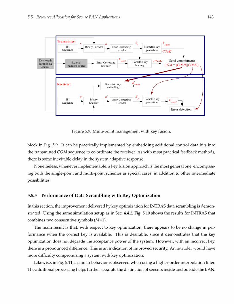
5.5. Resource Allocation for Secure BAN Applications 143
Figure 5.9: Multi-point management with key fusion.
block in Fig. 5.9. It can be practically implemented by embedding additional control data bits into
the transmitted COM sequence to co-ordinate the receiver. As with most practical feedback methods,
there is some inevitable delay in the system adaptive response.
Nonetheless, whenever implementable, a key fusion approach is the most general one, encompass-
ing both the single-point and multi-point schemes as special cases, in addition to other intermediate
possibilities.
5.5.5 Performance of Data Scrambling with Key Optimization
In this section, the improvement delivered by key optimization for INTRAS data scrambling is demon-
strated. Using the same simulation setup as in Sec. 4.4.2, Fig. 5.10 shows the results for INTRAS that
combines two consecutive symbols (M=1).
The main result is that, with respect to key optimization, there appears to be no change in per-
formance when the correct key is available. This is desirable, since it demonstrates that the key
optimization does not degrade the acceptance power of the system. However, with an incorrect key,
there is a pronounced difference. This is an indication of improved security. An intruder would have
more difficulty compromising a system with key optimization.
Likewise, in Fig. 5.11, a similar behavior is observed when using a higher-order interpolation filter.
The additional processing helps further separate the distinction of sensors inside and outside the BAN.

5.5. Resource Allocation for Secure BAN Applications 144
0 5 10 15 20 250
10
20
30
40
50
60
70
SNR (dB)
MS
E
Ideal key (from same sensor)Correct key (from same BSN)Incorrect key (without key optimization)Incorect key (with key optimization)
Figure 5.10: INTRAS Data Scrambling, with memory length M = 1.
And with the key optimization, an intruder would need to invest more resources to compromise the
system.
5.5.6 Performance of Data Scrambling using Variable-Size Block Construction
In Sec. 4.4.2, the effects of fading channels have been shown. Then, the variable-size block approach is
utilized to improve the performance by allocating the block-size according to the encountered channel.
For this simulation, the trunk-to-limb path, which is fast fading as surveyed in Sec. 4.1.11, is the channel
scenario for the three block processing schemes: fixed, variable and ideal.
The resulting performance with channel fading effects is shown in Fig. 5.12. It can be seen that with
a variable-size block, the MSE for the correct key is further reduced, approach that of the ideal scenario
with no channel estimation required (assuming prior channel knowledge). On the other hand, the
use of variable-size block has no major effect on the incorrect key performance. Since no major effect
implies that the MSE is not decreased, this is still a desirable effect. Indeed it means that an authorized
intruder does not have any benefit in attempting to compromise a variable-size block system for data
scrambling.

5.5. Resource Allocation for Secure BAN Applications 145
0 5 10 15 20 250
10
20
30
40
50
60
70
80
SNR (dB)
MS
E
Ideal key (from same sensor)Correct key (from same BSN)Incorrect key (without optimization)Incorect key (with key optimization)
Figure 5.11: INTRAS Data Scrambling, with memory length M = 3 using Lagrange interpolation.
5.5.7 Performance of the Key Fusion Scheme
In this final simulation, the utility of the fusion scheme for key distribution is illustrated. The results
without and with key fusion are shown for comparisons. In the key fusion scheme, half of the key bits
are derived from the biometrics, while the remaining from an external source. This implies that the
delay is reduced, as explained in Sec. 5.5.4.
The corresponding FRR/FAR performances are shown in Table 5.1.
The results for the key fusion scheme show little change compared to the key distribution from
only the biometrics. This is an indication that the biometrics are already providing a good degree of
randomness for key generation. If this were not the case, the external random source (which is forced
to generate statistically reliable random keys) would have resulted in significant improvement, since
it would provide a much improved source of randomness for the key. But according to the obtained
results, only slight changes are observed in the FAR. Therefore, when the biometrically driven keys are
already sufficient sources of randomness, the main advantage of the key fusion scheme is the trade-off
in delay. The cost to be paid is the increased computational complexity needed to generate the random
data bits.

5.6. Summary 146
0 5 10 15 20 250
10
20
30
40
50
60
70
SNR (dB)
MS
E
Incorrect key (fixed block)Incorrect key (variable block)Incorrect key (known channel)Correct key (fixed block)Correct key (variable block)Correct key (known channel)
Figure 5.12: INTRAS Data Scrambling using Variable-Size Block Construction, with memory length
M = 3 using Lagrange interpolation.
5.6 Summary
While all three classes of methods—being modeling, adaptation and integration—are all equally
important in contributing to the overall QoS performance, the integration category considered in
this chapter remains perhaps the least mature and reliable. This is due in part to its more recent
development, as well as to the difficulty and the number of unknowns and issues to be resolved.
When different methods are integrated, many variables can interact in unexpected manners. In cases
where the assumptions can be satisfied, the KKT approach delivers the optimal solutions. The mixed-
integer nature of the QoS problems is also accounted for, and handled with the branch-and-bound
algorithm.
Besides the difficulty of merely formulating the optimization problems (which need to be seman-
tically and numerically consistent with the application requirements), finding the solutions also poses
computational challenges. This chapter tackles several of these problems, including defining the QoS
requirements as a constrained optimization problem. However, there remain many outstanding re-
search problems to be considered in this area. With the framework established in this chapter as a

5.6. Summary 147
Parameters Without key fusion With key fusion
# subjects BCH Code # DET bits FRR (%) FAR (%) FRR (%) FAR (%)
24 (63,45,3) 64 15.6 0.02 14.7 0.02
24 (63,16,11) 64 4.5 0.02 4.2 0.02
24 (63,16,11) 32 4.7 0.03 4.4 0.02
40 (63,45,3) 64 17.1 0.03 16.6 0.03
40 (63,16,11) 64 5.1 0.03 4.8 0.03
40 (63,16,11) 32 5.3 0.04 5.0 0.03
Table 5.1: Performance of key generation and distribution at various coding conditions.
plausible stepping-stone, additional applications scenarios should be investigated besides those few
already explored here. For instance, case studies with different types of constraints, which mirror the
real-world environment, should provide invaluable insights. This endeavor should lead to challenging
but promising directions for future research in this area.

Chapter 6
Conclusion
6.1 General Summary
In this thesis, various signal processing methodologies have been proposed for constructing a uni-
fied QoS regulation framework for wireless networks that is both flexible (capable of accommodating
a wide range of operating conditions), and resource efficient (with reduced power and bandwidth
requirements, while still maintaining good QoS). These objectives are achieved by adapting the com-
munication system to the operating environment and envisioned application scenario. When the
encountered environment is benign, with good channel quality and modest QoS constraints, the more
resource-efficient modes of operation are invoked, e.g., less frequent channel tracking, and higher
throughput modulation schemes are used to conserve resources. On the other hand, when a more
challenging environment needs to be addressed, with hostile channel and stringent QoS constraints,
the more robust modes of operation are applied to maintain acceptable QoS.
Three main classes of methodologies are categorized: modeling, adaptation, and integration. These
categories roughly describes the hierarchical components of a successful QoS framework. Indeed, a
good system model is essential to effectively track the operating environment, so that subsequent
adaptation methods can response timely and deliver significant improvements. Furthermore, when
multiple methods are applied in a common network, a unified integration architecture is imperative
for achieving optimal overall gains.
Contributions are made in each of these areas throughout the thesis.
• In the modeling area, methods for accommodating different channel settings — frequency-
selective and time-selective, with various rates of fading — are proposed by adopting a variable
block fading model with multiple channel states. In particular, for cases of fast fading due to
high mobile velocity, a BEM channel is utilized to turn time-varying channel coefficients into
time-invariant state variables. Then, communications over rapidly fading channels can still be
148

6.1. General Summary 149
achieved reliably with practical hardware requirements. Notably, this also enables techniques
developed for time-invariant channels to still be applicable. And more importantly, this modeling
approach of characterizing multiple channel states is useful for tracking the channel quality so
that subsequent adaptation methods can be timely executed.
• In the adaptation area, the proposed methods have a common goal of improving the system
performance. However, each method typically operates at a particular communication layer,
and responds to different channel quality metric. Adaptation of training overhead focuses on
the channel rate of change: reduction of training density is possible whenever the channel
remains quasi-static over a sufficient amount of time. This is because the variable-size block can
deliver a higher effective amount of training to achieve comparable performance. In this manner,
bandwidth and power resources can be conserved. Similarly, adaptive modulation and coding
responds to the operating channel quality, quantified by the predicted BER performance, so that
highly efficient modes are used whenever the channel is benign. And for a multi-antenna system,
the antenna channel SNR is used to select the most favorable configuration. All together these
different methods all have the potential to regulate the QoS performance. However, to ensure
that the overall gain is consistently cumulative from the constituent methods, a framework with
well-defined objectives is needed — this area is precisely where the integration methods are
relevant.
• Furthermore, security is formulated as an important QoS aspect in the resource allocation frame-
work. Specifically the ECG biometric is utilized as a key enabling component to practically
implement security in the resource-constrained BAN. To this end, the coding scheme responds
to the detected channel quality in order to minimize the amount of information transmitted for
encryption key exchange. In addition, the alternative data scrambling based on random sam-
pling and interpolation provides a trade-off between computational and delay requirements.
• In the integration area, methods are proposed to enable effective integration of the adaptation
methods towards satisfying a common set of QoS constraints. This involves formulating an
equivalent nonlinear mathematical optimization problem. Practical aspects of translating the
optimal solution of the formulated problem into actual communication parameters are described.
For instance, the process of acquiring the state variables and feasible solution domain is facilitated
by the effective channel tracking and feedback components. Similarly, the adaptation methods
are designed to modify the system parameters, as dictated by the optimization solutions.
The obtained results demonstrate the benefits and future potentials of an integrated QoS frame-

6.2. Open Problems 150
work, where not only is each constituent method well-designed individually, but also the aggregation
of all methods is carefully tuned to sensible objectives and constraints. In this manner, various sce-
narios, with multiple users, applications and specific requirements, can be accommodated by the
framework.
One possible manner to collectively perceive and organize the methods proposed in this thesis is
illustrated in Fig. 6.1, where the roles of these methods are connected in the context of a unified QoS
framework.
Figure 6.1: Summary of contributions and their organization within a unified QoS framework.
6.2 Open Problems
In the context of delivering a successful and mature QoS architecture for wireless networks, many
important open problems still remain to be solved. Fortunately, due to its structured yet flexible nature,
the proposed framework is highly amenable to future upgrades. In fact, incremental modifications
can be made to any of the three identified areas, all so that an overall gain can be reaped in the whole
system. For example, a more robust channel tracking method will provide better estimates of the
operating channel quality. This in turn makes it possible for the subsequent adaptation methods to

6.2. Open Problems 151
adjust the system behavior in a more accurate manner. Similarly, a suitable channel metric would
make the selection of an optimal operating mode more reliable. And, certainly, advancements in the
algorithmic solutions of optimization problems would only result in a more resource-efficient QoS
architecture, with shorter delays and lower computational requirements.
In other words, improvements to any one of the aforementioned areas, including introduction of
new adaptation methods, can be absorbed into the QoS framework readily. In light of this advanta-
geous feature of the propose framework, the following incremental problems should merit particular
interest and attention to ameliorate the overall performance significantly.
• In the system modeling, selecting an appropriate method is important for achieving a balanced
trade-off in resources. While the BEM channel method represents a generalized method that can
be applied to a wide of scenarios, it may be unsuitable in a simple systems without significant
computational resources. As such, simplified channel models that take into account the specific
physical scenario of an application represents an important compromise in terms of resources
and QoS. For instance, if the mobile velocity is modest, the need to track the rapidly fading
channel components (which would be insignificant in this case), may be outweighed by other
design factors.
• For the channel tracking, improved methods for detecting changes in a time series, or for
process segmentation should be particularly useful. This is so that the operating channel state
can be detected more accurately for subsequent estimation and equalization. Consider the
analogy of a traffic control system, without reliable traffic light signals, the operations of various
vehicles within the system would cease to function properly. As such, the adaptive behaviors of
subsequent algorithms are highly dependent on a good channel tracking performance.
• More generally, other adaptation schemes which have not been studied in the thesis can be added
to provide extra degrees of freedom and better flexibility. For example, in chapter 3, the possibil-
ities of improved signal coding schemes have been suggested, with notations compatible with
MIMO formulation, so that space-time coding can be added later. Also, when multiple antennas
are not present physically, the strategy of coded cooperation can be used to let each cooperating
user act as a virtual antenna. These spatiotemporal processing schemes have the potential to
improve the system capacity and conserve resources even further. A future investigation of these
extensions is thus worthy of attention.
• With respect to the optimization architecture, alternative parametric characterizations of the
QoS should be useful to accommodate different applications. Constraints based on the data

6.2. Open Problems 152
rate or average BER may not be entirely appropriate. For example, in a scenario where the
short-term financial profit is the main criterion, trying to service as many users as possible may
be more viable. From an optimization perspective, these criteria are resolved by introducing
relevant variables and formulating suitable objective and constraint functions. However, once
formulated, the methods for solving the optimization problem can remain the same, with the
sequential procedure as outlined in chapter 5.
• Of course, fundamentally innovative solutions to constrained optimization problems can also
be absorbed into the whole QoS framework. This is particularly the case for the mixed-integer
optimization problems, where continued research is being actively conducted. Advances in these
fields should provide numerical algorithms with faster convergence and improved stability.
• Moreover, additional applications scenarios should be investigated besides those already ex-
plored in Sec. 5.3. Expanded case studies with different types of constraints, which mirror the
real-world environment, should provide invaluable insights. In particular, by revealing the
current strengths and weaknesses of the proposed framework, in addressing novel scenarios,
directions for future research may be more relevant and purposeful.
• The QoS framework considered is essentially a centralized architecture, where the assumption
of a powerful base station is made to coordinate other dependent network nodes according to an
optimization solution. An alternative architecture is one where various tasks are decentralized
into smaller subgroups. However, to accomplish this goal, advanced scheduling algorithms need
to be implemented in order to manage the networks in a transparent and structured manner for
efficiency [52]. This future direction represents an important step in improving the scalability
of the system, as well as alleviating the need of a virtually omnipresent and omnipotent base
station, which may not be a practical assumption in all cases.
• While the framework is capable of accommodating various security paradigms, only a limited
subset based on the ECG biometric for BAN has been explored. Investigating the system
performance with other security solutions should be an important next step. Furthermore,
while the ECG has been demonstrated as an apt class of signals for implementing secure key
exchanges, other physiological signals can also be examined. To this end, it should be recalled that
the necessary criteria include sufficient signal time-variance for randomness, and yet with good
recoverability for intra-class sensors. Preliminary investigations indicate that gait biometrics
may provide similar characteristics for BAN applications.
• An important criterion used to assess the merits of a proposed system is its real-world perfor-

6.2. Open Problems 153
mance. Most of the obtained results in the thesis have been based on simulation scenarios and
synthetic input data. Therefore verification of these results on prototype devices would provide
more rigor and insights to practical issues. Also, even for the biometric experiments, while
actual ECG signals were employed, these signals had been collected for different purposes. In
particular, due to the medical objectives involved, the time-invariant ECG features have been em-
phasized. However, for the BAN application, the time-variant features are of interest. Therefore,
an extensive data collection with a specialized setup should deliver more realistic performance
results.

Appendix A
Fundamentals of the Electrocardiogram
Electrocardiogram (ECG), also known as EKG (elektrokardiogramm), is basically a graph based on
the electrical activity of the heart. This versatile and important class of cardiac signals has a relatively
long and illustrious history. As a medical diagnostic technique, it was proposed by Willem Einthoven
in the early 1900s, and has since been acknowledged as an indispensable tool in the detection and
treatment of various cardiac disorders [45,134]. Among his many contributions, Einthoven was noted
for the currently used convention of assigning the letters P, Q, R, S and T to the various segments of
the ECG. For his discovery and pioneering work related to the ECG, Einthoven was recognized with
the 1924 Nobel Prize in Medicine.
More recently, as investigated in chapter 4, the ECG has fulfilled a rather unlikely niche, as a
purveyor of security and privacy in the form of a biometric [118, 145]. In this appendix, ECG fun-
damentals, especially characteristics and implications related to practical biometric signal processing
applications, are briefly reviewed.
A.1 Cardiovascular Physiology
From a gross anatomical perspective, the human heart can be considered a four-chambered muscular
blood pump [45,123]. The two top chambers are called the atria (left and right), while the bottom two
are called the ventricles (left and right). The ventricles are significantly larger (in volume and mass)
than the atria. As will be discussed, this difference will have notable implications on the intensity of
the signal observed, depending on its point of origin.
Together, the heart, arteries (vessels that carry blood away from the heart), veins (vessels that carry
blood back to the heart) and capillaries (microscopic blood vessels that connect the smallest arteries
to the smallest veins) are referred to as the cardiovascular system. Two cardiovascular divisions are
distinguished:
154

A.1. Cardiovascular Physiology 155
• Pulmonary circuit: consists mainly of the right side of the heart. It receives blood that has
circulated through the body, and carries this carbon dioxide loaded blood via the pulmonary
trunk, a large artery, to the lungs for gas exchange. Then the oxygen-rich blood travels back to
the heart via the pulmonary veins (on the left side).
• Systematic circuit: consists mainly the left side of the heart. The oxygenated blood leaves via
the aorta, a large artery, to supply blood to the organs in the body. After circulating through the
body, the now-deoxygenated blood returns to the heart (on the right side), via two large veins,
the superior vena cava (draining the upper body, including the thoracic organs) and the inferior
vena cava (draining organs below the diaphragm).
A.1.1 The Cardiac Conduction System
The heartbeat is myogenic, i.e., the control signals originate within the heart itself. The signals are
generated by the so-called pacemaker cells, which are specialized cardiac muscles. These cells are
auto-rhythmic and capable of generating action potentials [123]. Among the main organs comprising
the cardiac conduction system, controlling the routing and timing of electrical activities, the following
are particularly important.
• The sinoatrial (SA) node: the pacemaker site in the right atrium. It initiates each heartbeat and
regulates the heart rate. The signals originating from the SA node spread throughout the atria
to other sites.
• The atrioventricular (AV) node: located near the right AV valve, and acts as an electrical gateway
to the ventricles. Its fibrous and insulating skeleton ensures that it is the only path for currents
to travel to the ventricles.
A.1.2 The Electrical Activity of the Heart
The electrical events in the heart occur in a cycle of contraction (systole) and relaxation (diastole). When
the heartbeat occurs normally, as initiated by a healthy SA node, the regular heartbeat is called the
sinus rhythm, with a nominal rate of 70–80 beats per minute (bpm). However, this is highly dependent
on emotional factors, such as stress, anxiety, and shock, as well as on cardiovascular activities, such as
running and exercising.
With abnormal activities, the so-called cardiac arrhythmias occur, due to the depolarization trig-
gered by other regions than the normal pacemaker sites. Even though the SA node is the primary
pacemaker of the heart, depolarization can also be initiated by other areas with pacemaker potential,

A.2. The Electrocardiogram 156
e.g., by the autonomic foci: the atrial, junctional and ventrical foci. But in such cases, the ECG may
deviate from its normal healthy forms. Other conduction abnormalities may also cause disorders. For
all these pathological conditions, collectively known as arrhythmias, the heart rhythms can become
highly abnormal. Two categories are distinguished [45]:
• Sinus bradycardia: heart rate below the nominal sinus rhythm rate;
• Sinus tachycardia: heart rate above the nominal sinus rhythm rate.
A.2 The Electrocardiogram
The electrocardiogram is a depiction of the variations in the electrical potential of the heart over time.
As explained in the above, the change in voltage is due to the action potentials of cardiac cells. The
electrical activity is initiated when the sinoatrial (SA) node, the pacemaker of the heart, depolarizes.
This electrical signal then travels rhythmically until it reaches the atrioventricular (AV) node, which is
responsible for delaying the conduction rate, to properly pump blood from the atria into the ventricles.
The ECG signals are detected using electrodes or leads, which are attached to the skin. The signals
are amplified by an electrocardiograph. Simultaneous recordings from the electrodes are made; and,
at least for medical purposes, the displayed ECG is typically a composite or average of all action
potentials recorded.
A.2.1 ECG Events
In order to better delineate and demarcate an ECG, various signalling events are distinguished. It
should be noted that, while detailed guidelines exist on how the signal segmentation should be
achieved, there remains a great deal of variations and ambiguities in the procedure. Indeed, various
qualified personnel and certified equipment often deliver differing ECG segmentations. These dis-
crepancies have been acceptable in cardiac medical applications, which do not require highly precise
numerical quantifications. However, as discussed in chapter 4, biometric applications often impose
more stringent requirements. Fig. A.1 shows the salient components of an ECG segmentation, de-
picting the P wave, the QRS complex and the T wave (i.e., the Einthoven assignment mentioned
previously).
Together these events account for the sequential depolarization and repolarization of the heart.
• The P wave signals the activities from the SA node and atrial systole. It describes the depolar-
ization of the right and left atria. The amplitude of this wave is relatively small, because the

A.2. The Electrocardiogram 157
Figure A.1: Main components of an ECG heartbeat
atrial muscle mass is less significant compared to that of the ventricle. The absence of a P wave
typically indicates ventricular ectopic focus. This wave usually has a positive polarity, with a
duration of approximately 120 ms. In addition, its spectral content is limited to 10-15 Hz, i.e.,
low frequencies.
• The QRS complex corresponds to the largest wave, signalling ventricular systole (also atrial
repolarization). It represents the depolarization of the right and left ventricles, being the heart
chambers with substantial mass. The duration of this complex is approximately 70-110 ms in a
normal heartbeat. The anatomical characteristics of the QRS complex depend on the origin of
the pulse. Due to its steep slopes, the spectrum of a QRS wave is higher compared to that of
other ECG waves, and is mostly concentrated in the interval of 10-40 Hz.
• The T wave depicts the ventricular repolarization and diastole. It has a smaller amplitude, com-
pared to the QRS complex, and is usually observed 300 ms after this larger complex. However,
its precise position depends on the heart rate, e.g., appearing closer to the QRS waves at rapid
heart rates.
A.2.2 ECG Signal Acquisition and Noise Artifacts
Various electrodes placements and combinations are possible in ECG signal acquisition. The most
complete two-lead system in use includes:
• Bipolar Limb Leads: Lead I, Lead II, Lead III;

A.2. The Electrocardiogram 158
• Augmented Unipolar Limb Leads: aVR, aVR, aVR;
• Precordial Leads: V1, V2, V3, V4, V5, V6.
One of the main problems in biometric signal processing is the high degree of noise and variations.
In many cases, a reliable acquisition is only possible with sufficient knowledge of the spectral content,
the dynamic range and other characteristics of not only the desired signal components, but also of
the noise sources involved. This is so that the appropriate filters and quantizers can be accordingly
constructed to extract the desired signals, and reject the noise sources.
The previous section has highlighted the salient characteristics of ECG signal components. For
instance, the P wave is a lower-amplitude and lower-frequency signal, while the QRS complex exhibits
a larger amplitude and higher frequency variations. In addition, the following sources of noise and
artifacts are relevant to ECG. The baseline wander, arguably one of most common artifacts, refers to
a low-frequency interference in the ECG, which may be induced by cardiovascular activities. The
amplitude change due to baseline wander can potentially exceed the QRS amplitude by several times,
which can be highly problematic for accurate medical diagnoses based on the isoelectric line. While
this distortion may exhibit higher frequencies, e.g. during strenuous exercise, its spectral content is
typically limited to an interval below 1 Hz [134]. Thus, some type of low-pass filtering would be
relevant to this scenario.
Another source of error is powerline interference, being 50 or 60 Hz depending on the geographical
location, which occurs due to insufficient grounding or interferences from other equipments. Also
present in practical ECG recordings are electrode motion artifacts, due to skin stretching which alters
the impedance around the electrode. These artifacts are problematic since their spectral content, being
1-10 Hz, overlaps that of the desired signal components.
As well, there are inherent physiologically induced artifacts, viz., respiratory activity artifacts. The
involved chest movements change the position of the heart and the lung conductivity, leading to not
only variations in the heart rate, but also modifications of the beat morphology [134]. Clearly, as in
medical applications, an ECG-based biometric system needs to take into account all these various
sources of error, using the appropriate pre-processing, e.g., filtering based on the specific spectral
contents.
A.2.3 ECG Databases and Toolkits
Several public ECG databases can be found in the current literature. In this thesis, recorded signals
from the PhysioBank / PhysioNet project [53] were utilized for validating the proposed methods. This

A.2. The Electrocardiogram 159
project includes several sub-categories MIT-BIH, PTB, etc., each with a specific medical purpose, as
well as other types of physiological data besides ECG.
Also available from the PhysioNet project are open-source toolkits for visualizing and processing
the ECG. Several of these programs were utilized to handle ECG signals in this thesis, including:
• Chart-O-Matic: facilitates the display and visualization of ECG records;
• WFDB (waveform database): useful for manipulation of ECG records;
• ECGPUWAVE: a QRS detector, useful for fiducial applications.

Bibliography
[1] S. B. G. B. G. A. Scaglione, P. Stoica and H. Sampath, “Optimal designs for space-time linear
precoders and equalizers,” IEEE Trans. Signal Processing, vol. 50, pp. 1051–1064, May 2002.
[2] S. A. Ahson and M. Ilyas, WiMAX: Technologies, Performance Analysis, and QoS. CRC, 2007.
[3] I. F. Akyildiz, W. Su, Y. Sankarasubramaniam, and E. Cayirci, “A survey on sensor networks,”
IEEE Commun. Mag., pp. 102–114, Aug. 2002.
[4] E. Alsusa and L. Yang, “Novel low-complexity post-IFFT PAPR reduction technique for OFDM
systems,” in Proc. IEEE WCNC 2006, 2006, pp. 2006–2011.
[5] H. Arslan, “Adaptation techniques and enabling parameter estimation algorithms for wireless
communications systems,” in Signal Processing for Mobile Communications, M. Ibnkahla, Ed. CRC
Press, 2004.
[6] P. Balaban and J. Salz, “Optimum diversity combining and equalization in digital data trans-
mission with applications to cellular mobile radio — part i: Theoretical considerations,” IEEE
Trans. Commun., pp. 885–894, 1992.
[7] S. Bao, Y. Zhang, and L. Shen, “A novel key distribution of body area networks for telemedicine,”
in Proc. IEEE Workshop on Biomedical Circuits and Systems, 2004.
[8] ——, “A new symmetric cryptosystem of body area sensor networks for telemedicine,” in Proc.
of the 6th Asian-Pacific Conference on Medical and Biological Engineering, Apr. 2005.
[9] ——, “Physiological signal based entity authentication for body area sensor networks and mobile
healthcare systems,” in Proc. 27th EMBS Annual International Conference of the IEEE, 2005, pp.
2455–2458.
[10] I. Barhumi, G. Leus, and M. Moonen, “Time-varying FIR equalization for doubly selective
channels,” IEEE Trans. Wireless Commun., no. 1, pp. 202–214, Jan. 2005.
160

Bibliography 161
[11] M. Basseville, “Detecting changes in signals and systems – a survey,” Automatica, vol. 24, no. 3,
pp. 309–326, 1988.
[12] M. S. Bazaraa, H. D. Sherali, and C. M. Shetty, Nonlinear Programming: Theory and Algorithms.
Wiley-Interscience.
[13] P. A. Bello, “Characterization of randomly time-variant linear channels,” IEEE Trans. on Commu-
nication Systems, vol. CS-11, no. 4, pp. 360–393, Dec. 1963.
[14] R. Berezdivin, R. Breinig, and R. Topp, “Next-generation wireless communications concepts and
technologies,” IEEE Commun. Mag., vol. 40, no. 3, pp. 108–116, 2002.
[15] R. A. Berry and E. M. Yeh, “Cross-layer wireless resource allocation,” IEEE Signal Processing
Mag., vol. 21, no. 5, pp. 59–68, 2004.
[16] M. A. Bhatti, Practical Optimization Methods: With Mathematica Applications. Springer Telos,
2000, ISBN: 0387986316.
[17] L. Biel, O. Pettersson, L. Philipson, and P. Wide, “ECG analysis: a new approach in human
identification,” IEEE Trans. on Instrumentation and Measurement, vol. 50, no. 3, pp. 808–812, 2001.
[18] J. Blogh and L. Hanzo, Third-Generation Systems and Intelligent Wireless Networking: Smart Anten-
nas and Adaptive Modulation. John Wiley, 2002.
[19] H. Boche, M. Wiczanowski, and S. Stanczak, “Characterization of optimal resource allocation in
cellular networks,” in Proc. SPAWC2004, 2004.
[20] S. P. Boyd and L. Vandenberghe, Convex Optimization. Cambridge, UK: Cambridge University
Press, 2004, ISBN: 0521833787.
[21] F. M. Bui, F. Agrafioti, and D. Hatzinakos, “Electrocardiogram (ECG) biometric for robust iden-
tification and secure communication,” in Biometrics: Theory, Methods and Applications, N. Boul-
gouris, E. Micheli-Tzanakou, and K. Plataniotis, Eds. Wiley/IEEE, (to appear).
[22] F. M. Bui and D. Hatzinakos, “A receiver-based variable-size-burst equalization strategy for
spectrally efficient wireless communications,” IEEE Trans. Signal Processing, vol. 53, no. 11, pp.
4304–4314, Nov. 2005.
[23] ——, “Identification and tracking of rapidly time-varying mobile channels for improved equal-
ization: A basis-expansion model approach,” in Proc. CSNDSP 2006, Patras, Greece, July 2006.

Bibliography 162
[24] ——, “Spectrally efficient communication over time-varying frequency-selective mobile chan-
nels: Variable-size burst construction and adaptive modulation,” EURASIP Journal on Applied
Signal Processing, Special Issue on Reliable Communications over Rapidly Time-Varying Channels, pp.
1–16, 2006, Article ID 35352.
[25] ——, “An interpolation and resampling framework for efficient reduction of peak-to-average
power ratio in OFDM systems,” in Proc. IEEE PIMRC 2007, Athens, Greece, Sept. 2007.
[26] ——, “Resource allocation strategies for secure and efficient communications in biometrics-
based body sensor networks,” in Proc. of Biometrics Symposiums (BSYM), Baltimore, Maryland,
USA, September 2007.
[27] ——, “Biometric methods for secure communications in body sensor networks: Resource-
efficient key management and signal-level data scrambling,” EURASIP Journal on Advances
in Signal Processing, Special Issue on Advanced Signal Processing and Pattern Recognition Methods for
Biometrics, pp. 1–16, 2008, Article ID 529879.
[28] ——, “Secure methods for fuzzy key binding in biometric authentication applications,” in Proc.
Asilomar Conference on Signals, Systems, and Computers, Pacific Groove, CA, USA, Oct. 2008.
[29] P. Campisi, M. Carli, G. Giunta, and A. Neri, “Blind quality assessment system for multimedia
communicatiosn using tracing watermarking,” IEEE Trans. Signal Processing, vol. 51, no. 4, pp.
996–1002, 2003.
[30] S. Catreux, V. Erceg, D. Gesbert, and R. W. Heath, “Adaptive modulation and MIMO coding for
broadband wireless data networks,” IEEE Commun. Mag., vol. 40, no. 6, pp. 108–115, June 2002.
[31] A. Cavoukian and A. Stoianov, “Biometric encryption: A positive-sum technology that achieves
strong authentication, security and privacy,” Information and Privacy Commissioner/Ontario, Mar.
2007.
[32] H. Chen, Radio resource management for multimedia QoS support in wireless networks. Boston:
Kluwer Academic Publishers, 2004, ISBN: 1402076231.
[33] S. Cherukuri, K. K. Venkatasubramanian, and S. K. S. Gupta, “Biosec: A biometric based ap-
proach for securing communication in wireless networks of biosensors implanted in the human
body,” in Proc. IEEE Conf. Parallel Processing Wksp., 2003, pp. 432–39.
[34] S. Coleri, M. Ergen, A. Puri, and A. Bahai, “Channel estimation techniques based on pilot
arrangement in OFDM systems,” IEEE Trans. Broadcast., vol. 48, pp. 223–229, Sept. 2002.

Bibliography 163
[35] S. N. Diggavi, N. Al-Dhahir, A. Stamoulis, and A. R. Calderbank, “Great expectations: The value
of spatial diversity in wireless networks,” Proc. IEEE, vol. 92, no. 2, pp. 219–270, Feb. 2004.
[36] M. Dong and L. Tong, “Optimal placement of training for channel estimation and tracking,” in
Proc. MILCOM, 2001, pp. 1195–1199.
[37] ——, “Optimal design and placement of pilot symbols for channel estimation,” IEEE Trans.
Signal Processing, pp. 3055–3069, 2002.
[38] Z. Du, N. Beaulieu, and J. Zhu, “Reduced complexity peak-to-average power ratio reduction for
OFDM by selective time domain filtering,” in Proc. IEEE Globecom 2005, 2005, pp. 2802–2806.
[39] G. Eichfeld, Adaptive Scalarization Methods in Multiobjective Optimization. Springer, 2008.
[40] A. Eisenblatter and H.-F. Geerdes, “Wireless network design: Solution-oriented modeling and
mathematical optimization,” IEEE Trans. Wirel. Comm.: 3G/4G/WLAN/WMAN Planning and Opti-
mization, pp. 8–14, Dec. 2006.
[41] C. A. Floudas, Nonlinear and Mixed-Integer Optimization: Fundamentals and Applications. Oxford
University Press, 1995.
[42] A. Fort, C. Desset, J. Ryckaert, P. De Doncker, L. Van Biesen, and S. Donnay, “Ultra wide-band
body area channel model,” in 2005 IEEE International Conference on Communications (ICC 2005),
2005.
[43] A. Fort, C. Desset, J. Ryckaert, P. Doncker, L. V. Biesen, and P. Wambacq, “Characterization of
the ultra wideband body area propagation channel,” in Int. Conference on Ultra Wideband (ICU),
Sept. 2005.
[44] G. Foschini, “Layered space-time architecture for wireless communication in a fading environ-
ment when using multi-element antennas,” Bell Labs Tech. J., vol. 1, no. 2, p. 4159, Sept. 1996.
[45] D. B. Foster, Twelve-Lead Electrocardiography: Theory and Interpretation, 2nd ed. Springer, 2007.
[46] M. Gen, R. Cheng, and L. Lin, Network Models and Optimization: Multiobjective Genetic Algorithm
Approach. Springer, 2008.
[47] G. B. Giannakis, P. A. Anghel, and Z. Wang, “Wideband generalized multi-carrier CDMA over
frequency-selective wireless channels,” in Proc. IEEE ICASSP 2000, 2000, pp. 2501–2504.

Bibliography 164
[48] ——, “Generalized multi-carrier CDMA: Unification and linear equalization,” EURASIP Journal
on Applied Signal Processing, pp. 743–756, 2005.
[49] G. B. Giannakis and C. Tepedelenlioglu, “Basis expansion models and diversity techniques for
blind identification and equalization of time-varying channels,” Proc. IEEE, no. 10, pp. 1969–
1986, Oct. 1998.
[50] G. Giunta, “Quality of service assessment in new generation wireless video communications,”
in SDigital Image Sequence Processing: Compression and Analysis, T. Reed, Ed. CRC press, 2004.
[51] S. G. Glisic, Advanced Wireless Communications: 4G Technologies, 1st ed. Wiley, 2004.
[52] ——, Advanced Wireless Networks: 4G Technologies. Wiley, 2006.
[53] A. L. Goldberger, L. A. N. Amaral, L. Glass, J. M. Hausdorff, P. C. Ivanov, R. G. Mark,
J. E. Mietus, G. B. Moody, C.-K. Peng, and H. E. Stanley, “PhysioBank, PhysioToolkit,
and PhysioNet: Components of a new research resource for complex physiologic signals,”
Circulation, vol. 101, no. 23, pp. e215–e220, 2000 (June 13), circulation Electronic Pages:
http://circ.ahajournals.org/cgi/content/full/101/23/e215.
[54] D. A. Gore and A. J. Paulraj, “MIMO antenna subset selection with space-time coding,” IEEE
Trans. Signal Processing, vol. 50, no. 10, 2002.
[55] P. S. Hall and Y. Hao, Antennas and Propagation for Body-Centric Wireless Communications. Artech
House, 2006.
[56] S. H. Han and J. H. Lee, “An overview of peak-to-average power ratio reduction techniques for
multicarrier transmission,” IEEE Trans. Wireless Commun., vol. 12, no. 2, pp. 56–65, Apr. 2005.
[57] Z. Han, X. Liu, Z. J. Wang, and K. J. R. Liu, “Delay sensitive scheduling schemes for heterogeneous
qos over wireless networks,” IEEE Trans. Wireless Commun., vol. 6, pp. 423–428, Feb. 2007.
[58] L. Hanzo, T. H. Liew, and B. L. Yeap, Turbo Coding, Turbo Equalisation and Space-Time Coding for
Transmission over Fading Channels. John Wiley, 2002, ISBN: 0470847263.
[59] L. Hanzo, W. Webb, and T. Keller, Single- and Multi-carrier Quadrature Amplitude Modulation:
Principles and Applications for Personal Communications, WLANs and Broadcasting. John Wiley,
2000.
[60] L. Hanzo, C. Wong, and M. Yee, Adaptive Wireless Transceivers: Turbo-Coded, Turbo-Equalized and
Space-Time coded TDMA, CDMA, and OFDM Systems. John Wiley, 2002.

Bibliography 165
[61] L. Hanzo, L. Yang, E. Kuan, and K. Yen, Single and Multi-Carrier DS-CDMA: Multi-User Detec-
tion, Space-Time Spreading, Synchronisation, Networking and Standards. John Wiley, 2003, ISBN:
0470863099.
[62] S. Haykin, Adaptive Filter Theory. Prentice Hall, 1996.
[63] S. Haykin and M. Moher, Modern Wireless Communication. Prentice Hall, 2004, ISBN: 0130224723.
[64] W. R. Heinzelman, A. Chandrakansan, and H. Balakrishnan, “Energy-efficient communication
protocol for wireless microsensor networks,” in Proc. of the 33rd Hawaii International Conference
on System Science, Hawaii, USA, 2000.
[65] A. Hottinen, O. Tirkkonen, and R. Wichman, Multi-antenna Transceiver Techniques for 3G and
Beyond. John Wiley, 2003, ISBN: 0470845422.
[66] Z. H. Hu, Y. I. Nechayev, P. S. Hall, C. C. Constantinou, and Y. Hao, “Measurements and statistical
analysis of on-body channel fading at 2.45 ghz,” IEEE Antennas Wireless Propagat. Lett., vol. 6,
pp. 612–615, 2007.
[67] V. Huang and W. Zhuang, “QoS-oriented access control for 4g mobile multimedia CDMA
communications,” IEEE Commun. Mag., vol. 40, no. 4, pp. 118–125, Mar. 2002.
[68] IEEE, “The IEEE 802.15 task group 6: Body area networks (BAN),” IEEE Wireless PAN, 2008,
bAN Homepage: http://www.ieee802.org/15/pub/TG6.html.
[69] M. Ilyas, Ed., The Handbook of Ad Hoc Wireless Networks. CRC Press, 2003.
[70] S. A. Israel, J. M. Irvine, A. Cheng, M. D. Wiederhold, and B. K. Wiederhold, “ECG to identify
individuals,” Pattern Recognition, vol. 38, no. 1, pp. 133–142, 2005.
[71] S. A. Israel, W. T. Scruggs, W. J. Worek, and J. M. Irvine, “Fusing face and ECG for personal
identification,” in Proc. of 32nd Applied Imagery Pattern Recognition Workshop, 2003, pp. 226–231.
[72] A. K. Jain, A. Ross, and S. Prabhakar, “An introduction to biometric systems,” IEEE Transactions
on Circuit and Systems for Video Technology, vol. 14, no. 1, pp. 4–20, 2004.
[73] M. Janani, A. Hedayat, T. Hunter, and A. Nosratinia, “Coded cooperation in wireless communi-
cations: Space-time transmission and iterative decoding,” IEEE Trans. Signal Processing, vol. 52,
no. 2, pp. 362–371, Feb. 2004.

Bibliography 166
[74] U. S. Jha and R. Prasad, OFDM Towards Fixed and Mobile Broadband Wireless Access. Artech
House, 2007, ISBN: 9781580536417.
[75] A. Juels and M. Sudan, “A fuzzy vault scheme,” in Proceedings 2002 IEEE International Symposium
on Information Theory, 2002.
[76] A. Juels and M. Wattenberg, “A fuzzy commitment scheme,” in Proc. 6th ACM Conf. Comp. and
Commun. Sec., 1999, pp. 28–36.
[77] G. Kabatiansky, E. Krouk, and S. Semenov, Error Correcting Coding and Security for Data Networks:
Analysis of the Superchannel Concept. John Wiley and Sons, 2005.
[78] V. Kawadia and P. Kumar, “A cautionary perspective on cross-layer design,” IEEE Trans. Wireless
Commun., vol. 12, pp. 3–11, Feb. 2005.
[79] S. M. Kay, Fundamentals of Statistical Signal Processing: Estimation Theory, 1st ed. Prentice Hall,
1993.
[80] C.-C. J. Kuo, S.-H. Tsai, L. Tadjpour, and Y.-H. Chang, Precoding Techniques for Digital Communi-
cation Systems. Springer, 2008.
[81] S. A. Kyriazakos and G. T. Karetsos, Practical Radio Resource Management in Wireless Systems.
Artech House, 2004.
[82] J. N. Laneman and G. W. Wornell, “Distributed space-time coded protocols for exploiting coop-
erative diversity in wireless networks,” IEEE Trans. Inform. Theory, vol. 49, no. 10, pp. 2415–2525,
Oct. 2003.
[83] E. G. Larsson, P. Stoica, and G. Ganesan, Space-Time Block Coding for Wireless Communications.
Cambridge University Press, 2003, ISBN: 0521824567.
[84] V. K. Lau and Y. K. R. Kwok, Channel-Adaptive Technologies and Cross-Layer Designs for Wireless
Systems with Multiple Antennas: Theory and Applications. Wiley-Interscience, 2006.
[85] M. Lavielle, “Optimal segmentation of random processes,” IEEE Trans. Signal Processing, vol. 46,
no. 5, pp. 1365–1373, May 1998.
[86] K. Letaief and Y. J. Zhang, “Dynamic multiuser resource allocation and adaptation for wireless
systems,” IEEE Wireless Communications, pp. 38–47, Aug. 2007.

Bibliography 167
[87] G. Leus, S. Zhou, and G. B. Giannakis, “Orthogonal multiple access over time- and frequency-
selective channels,” IEEE Trans. Inform. Theory, no. 8, pp. 1942–1950, Aug. 2003.
[88] D. Li and X. Sun, Nonlinear Integer Programming. Springer, 2006.
[89] Z. Liu, A. Scaglione, S. Barbarossa, and G. Giannakis, “Block spacetime antenna precod-
ing/decoding for generalized multicarrier communications in unknown multipath,” in Proc.
of 37th Annual Allerton Conf. on Communication, Control, and Computing.
[90] Z. Liu, G. B. Giannakis, S. Barbarossa, and A. Scaglione, “Transmit-antennae space-time block
coding for generalized OFDM in the presence of unknown multipath,” IEEE J. Select. Areas
Commun., vol. 19, 2001.
[91] J. Lopez and J. Zhou, Wireless Sensor Network Security. IOS Press, 2008.
[92] S. Lu, J. Kanters, and K. H. Chon, “A new stochastic model to interpret heart rate variability,” in
Proc. 25th EMBS Annual International Conference of the IEEE, 2003, pp. 17–21.
[93] D. G. Luenberger and Y. Ye, Linear and Nonlinear Programming, 3rd ed. Springer, 2008.
[94] X. Ma, G. B. Giannakis, and S. Ohno, “Optimal training for block transmissions over doubly
selective wireless fading channels,” IEEE Trans. Signal Processing, pp. 1351–1366, May 2003.
[95] J. Malmivuo and R. Plonsey, Bioelectromagnetism: Principles and Applications of Bioelectric and
Biomagnetic Fields. New York: Oxford University Press, 1995.
[96] D. Manocha, “Solving systems of polynomial equations,” IEEE Comput. Graph. Appl., pp. 46–55,
1994.
[97] F. Marvasti, Nonuniform Sampling: Theory and Practice. Kluwer Academic/Plenum Publishers,
2001.
[98] A. J. Menezes, P. C. van Oorschot, and S. A. Vanstone, Handbook of Applied Cryptography. CRC
Press, 1996.
[99] F. Meshkati, H. V. Poor, and S. C. Schwartz, “Energy-efficient resource allocation in wireless
networks: An overview of game-theoretic approaches,” IEEE Signal Processing Mag., pp. 58–68,
May 2007.
[100] A. Mishra, Security and Quality of Service in Ad Hoc Wireless Networks. Cambridge University
Press, 2008.

Bibliography 168
[101] S. Misra, A. Swami, , and L. Tong, “Optimal training for time-selective wireless fading channels
using cutoff rate,” EURASIP Journal on Applied Signal Processing, pp. 1–15, 2006, Article ID 47245.
[102] V. Mitlin, Performance Optimization of Digital Communications Systems. Auerbach Publications,
2006.
[103] E. Modiano, “An adaptive algorithm for optimizing the packet size used in wireless ARQ
protocols,” Wireless Networks, vol. 5, pp. 279–286, 1999.
[104] A. F. Molisch, Wideband Wireless Digital Communications. Prentice Hall, 2001.
[105] S. Nanda, K. Balachandran, and S. Kumar, “Adaptation techniques in wireless packet data
services,” IEEE Commun. Mag., vol. 38, no. 1, pp. 54–64, Jan. 2000.
[106] Y. Nechayev, P. Hall, C. Constantinou, Y. Hao, A. Alomainy, R. Dubrovka, and C. Parini, “On-
body path gain variations with changing body posture and antenna position,” in IEEE Antennas
and Propagation Society International Symposium, 2005.
[107] M. Niedzwiecki, Identification of Time-Varying Processes. John Wiley, 2000.
[108] B. Noble and J. Daniel, Applied Linear Algebra, 3rd ed. Prentice Hall, 1987.
[109] J. Nocedal and S. Wright, Numerical Optimization: Theoretical and Practical Aspects. Springer,
2006.
[110] A. Nosratinia and A. Hedayat, “Cooperative communication in wireless networks,” IEEE Com-
mun. Mag., Oct. 2004.
[111] A. V. Oppenheim, R. W. Schafer, and J. R. Buck, Discrete-Time Signal Processing, 2nd ed. New
Jersey: Prentice Hall, 1999.
[112] R. G. Parker and R. L. Rardin, Discrete Optimization. Academic Press, 1988.
[113] M. Patzold, Mobile Fading Channels. John Wiley, 2002.
[114] A. Paulraj, R. Nabar, and D. Gore, Introduction to Space-Time Wireless Communications. Cambridge
University Press, 2003, ISBN: 0521826152.
[115] A. J. Paulraj and C. B. Papadias, “Space-time processing for wireless communications: Improving
capacity, coverage and quality in wireless communications by exploiting the spatial dimension,”
IEEE Signal Processing Mag., vol. 14, no. 6, pp. 49–83, Nov. 1997.
Bibliography 169
[116] A. Perrig, R. Szewczyk, J. Tygar, V. Wen, and D. E. Culler, “SPINS: Security protocols for sensor
networks,” Wireless Networks, vol. 8, no. 5, pp. 521–534, Sept. 2002.
[117] K. N. Plataniotis, D. Hatzinakos, and J. K. M. Lee, “ECG biometric recognition without fiducial
detection,” in Proc. of Biometrics Symposiums (BSYM), Baltimore, Maryland, USA, September
2006.
[118] C. Poon, Y.-T. Zhang, and S.-D. Bao, “A novel biometrics method to secure wireless body area
sensor networks for telemedicine and m-health,” IEEE Commun. Mag., pp. 73–81, Apr. 2006.
[119] J. G. Proakis, Digital Communications, 4th ed. McGraw Hill, 2001.
[120] Q. M. Rahman and M. Ibnkahla, “Signal processing for future mobile communications systems:
Challenges and perspectives,” in Signal Processing for Mobile Communications, M. Ibnkahla, Ed.
CRC Press, 2004.
[121] R. M. Rao, C. Comaniciu, T. Lakshman, and H. V. Poor, “Call admission control in wireless
multimedia networks,” IEEE Signal Processing Mag., vol. 21, no. 5, pp. 51–58, 2004.
[122] T. S. Rappaport, Wireless Communications: Principles and Practice. Prentice Hall, 1996.
[123] K. S. Saladin, Anatomy and Physiology: The Unity of Form and Function. McGraw-Hill, 2004.
[124] S. Sanayei and A. Nosratinia, “Antenna selection in MIMO systems,” IEEE Commun. Mag., pp.
68–73, Oct. 2004.
[125] C. Saraydar, N. Mandayam, and D. Goodman, “Efficient power control via pricing in wireless
data networks,” IEEE Trans. Commun., vol. 50, pp. 291–303, Feb. 2002.
[126] A. Shamir, “How to share a secret,” Communications of the ACM, vol. 22, no. 1, pp. 612–613, 1979.
[127] V. Shankar, A. Natarajan, S. K. S. Guptar, and L. Schwiebert, “Energy-efficient protocols for
wireless communication in biosensor networks,” in IEEE Personal, Indoor and Mobile Radio Com-
munications Conference, San Diego, 2001.
[128] T. W. Shen, “Biometric identity verification based on electrocardiogram (ECG),” Ph.D. disserta-
tion, University of Wisconsin, Madison, 2005.
[129] T. W. Shen, W. J. Tompkins, and Y. H. Hu, “One-lead ECG for identity verification,” in Proc. of
the 2nd Conf. of the IEEE Eng. in Med. and Bio. Society and the Biomed. Eng. Society, vol. 1, 2002, pp.
62–63.

Bibliography 170
[130] D. Soldani and K. Valkealahti, “Genetic approach to QoS optimization for WCDMA mobile
networks,” in Vehicular Technology Conference, 2005, 2005, pp. 2269–2273.
[131] D. Soldani, M. Li, and R. Cuny, QoS and QoE Management in UMTS Cellular Systems. John Wiley
& Sons, 2006.
[132] G. Song and Y. G. Li, “Cross-layer optimization for OFDM wireless networks - part i: Theoretical
framework,” IEEE Trans. Wireless Commun., vol. 4, no. 2, pp. 614–624, Mar. 2005.
[133] ——, “Cross-layer optimization for OFDM wireless networks - part ii: Algorithm development,”
IEEE Trans. Wireless Commun., vol. 4, no. 2, pp. 625–634, Mar. 2005.
[134] L. Sornmo and P. Laguna, Bioelectrical Signal Processing in Cardiac and Neurological Applications.
Elsevier, 2005.
[135] W. Stallings, Cryptography and Network Security: Principles and Practice, 4th ed. New Jersey:
Prenticall Hall, 2006.
[136] R. Steele and L. Hanzo, Mobile Radio Communications: Second and Third Generation Cellular and
WATM Systems. John Wiley, 1999.
[137] R. K. Sundaram, A First Course in Optimization Theory. Cambridge University Press, 1996.
[138] I. E. Telatar, “Capacity of multiple antenna gaussian channels,” Eur. Trans. Telecommun., vol. 10,
no. 6, pp. 585–595, Nov./Dec. 1999.
[139] C. Tellambura, “Computation of the continuous-time PAR of an OFDM signal with BPSK sub-
carriers,” IEEE Commun. Lett., vol. 5, no. 5, pp. 185–187, May 2001.
[140] V. Valimaki, T. Tolonen, and M. Marjalainen, “Signal-dependent nonlinearities for physical mod-
els using time-varying fractional delay filters,” in Proc. International Computer Music Conference,
1998, pp. 264–267.
[141] M. van der Schaar, S. Krishnamachari, S. Choi, and X. Xu, “Adaptive cross-layer protection
strategies for robust scalable video transmission over 802.11 wlans,” IEEE J. Select. Areas Com-
mun., vol. 21, no. 10, pp. 1752– 1763, Dec. 2003.
[142] M. van Der Schaar and N. S. Shankar, “Cross-layer wireless multimedia transmission: challenges,
principles, and new paradigms,” IEEE Trans. Wireless Commun., vol. 12, pp. 50–58, Aug. 2005.

Bibliography 171
[143] M. van der Schaar and D. S. Turaga, “Cross-layer packetization and retransmission strategies for
delay-sensitive wireless multimedia transmission,” IEEE Trans. Multimedia, vol. 9, pp. 185–197,
2007.
[144] P. K. Varshney, Distributed detection and data fusion. NY: Springer, 1997, ISBN: 0387947124.
[145] K. K. Venkatasubramanian and S. K. S. Gupta, “Security for pervasive health monitoring sensor
applications,” in Proc. of 4th International Conference on Intelligent Sensing and Information Processing
(ICISIP), 2006.
[146] H. Vikalo, B. Hassibi, B. Hochwald, and T. Kailath, “Optimal training for frequency-selective
fading channels,” in Proc. IEEE International Conference on ASSP, 2001, pp. 2105–2108.
[147] B. Vucetic and J. Yuan, Space-Time Coding. John Wiley, 2003, ISBN: 0470847573.
[148] X. Wang and H. V. Poor, Wireless Communication Systems: Advanced Techniques for Signal Reception.
Prentice Hall PTR, 2003, ISBN: 0130214353.
[149] Y. Wang, F. Agrafioti, D. Hatzinakos, and K. Plataniotis, “Analysis of human electrocardiogram
(ECG) for biometric recognition,” EURASIP Journal on Advances in Signal Processing, 2007.
[150] Y. Wang, K. N. Plataniotis, and D. Hatzinakos, “Integrating analytic and appearance attributes
for human identification from ECG signal,” in Proc. of Biometrics Symposiums (BSYM), Baltimore,
Maryland, USA, September 2006.
[151] Z. Wang and G. B. Giannakis, “Wireless multicarrier communications: Where Fourier meets
Shannon,” IEEE Signal Processing Mag., pp. 29–48, May 2000.
[152] ——, “A simple and general approach to the average and outage performance analysis in
fading,” IEEE Trans. Commun., vol. 51, pp. 1389–1398, Aug. 2003.
[153] C. H. Wong and L. Hanzo, “Upper-bound performance of a wide-band adaptive modem,” IEEE
Trans. Commun., vol. 48, no. 3, pp. 367–369, Mar. 2000.
[154] C. Y. Wong, R. S. Cheng, K. B. Letaief, and R. D. Murch, “Multiuser ofdm with adaptive subcarrier,
bit and power allocation,” IEEE J. Select. Areas Commun., vol. 17, no. 10, pp. 1747–1758, 1999.
[155] I. Wong and B. Evans, Resource Allocation in Multiuser Multicarrier Wireless Systems. Springer,
2007.
[156] G.-Z. Yang, Ed., Body Sensor Networks. Springer, 2006.

Bibliography 172
[157] S. Yang and I. Verbauwhede, “Secure fuzzy vault based fingerprint verification system,” in
Thirty-Eighth Asilomar Conference on Signals, Systems, and Computers, 2004.
[158] K. Y. Yazdandoost, H. Sawada, S. T. Choi, J. ichi Takada, and R. Kohno, “Channel characterization
for BAN communications,” in IEEE 802.15-07-0641-00-0ban, Mar. 2007.
[159] S. Yoo, S. Yoon, S. Y. Kim, and I. Song, “A novel PAPR reduction scheme for OFDM systems:
Selective mapping of partial tones (SMOPT),” IEEE Trans. Consumer Electron., vol. 52, no. 1, pp.
40–43, Feb. 2006.
[160] C. J. Zarowski, An Introduction to Numerical Analysis for Electrical and Computer Engineers. Wiley-
Interscience, 2000.
[161] R. Ziegler and J. Cioffi, “Estimation of time-varying digital radio channels,” IEEE Trans. Veh.
Technol., vol. 41, no. 2, pp. 134–151, May 1992.