Signal, Instruments and SystemsProject 5:

Sensor accuracy in environmental sensor networks

IntroductionWe deal with the important question of calibration of sensor

devices. Here we focuse on the Mica-Z temperature sensor.

How can we obtain the best accuracy limiting the costs ?

I. Experiments to collect data

II. Methods of calibration : the interpolating polynomial

III. Results

IV. Difficulties met and observations

Experiments done

Differents experiments : at ambiant temperature cooling (1) fast heating (2) cooling and then smooth heating (3)

First results : reference data always under the measured one. the gap between the two raised at the extremes.

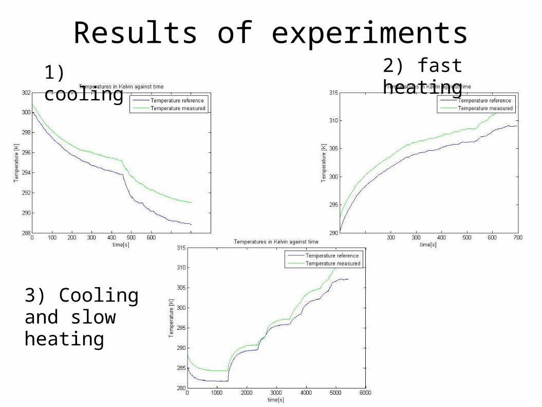
Results of experiments1) cooling 2) fast heating

3) Cooling and slow heating

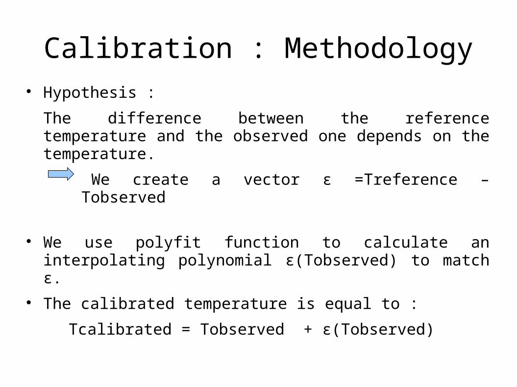
Calibration : Methodology Hypothesis :

The difference between the reference temperature and the observed one depends on the temperature.

We create a vector ε =Treference – Tobserved

We use polyfit function to calculate an interpolating polynomial ε(Tobserved) to match ε.

The calibrated temperature is equal to :

Tcalibrated = Tobserved + ε(Tobserved)

Calibration : The interpolating polynomial

For each set of data collected, we create several polynomials of different degrees.

We compare them. The final choice of the experiment and the degree used are

experimental.

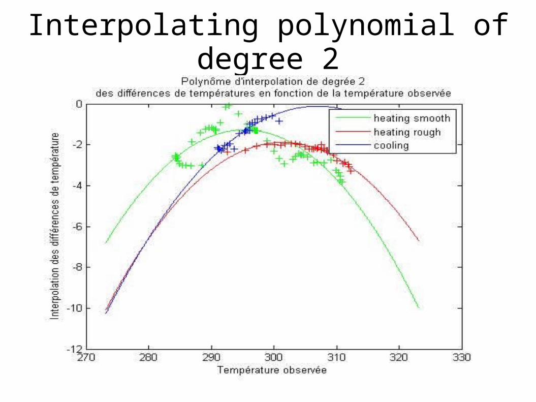
Interpolating polynomial of degree 2

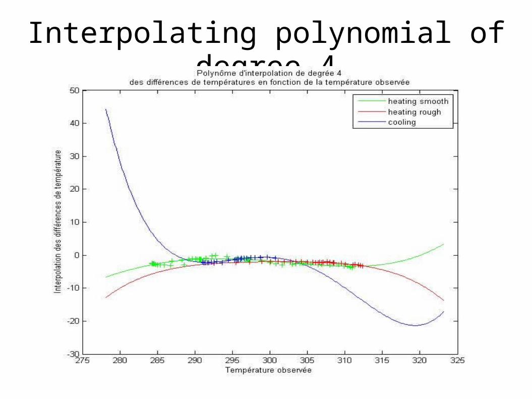
Interpolating polynomial of degree 4

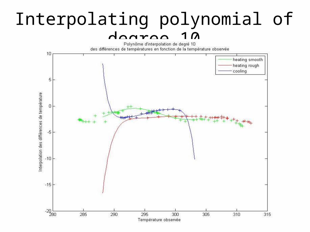
Interpolating polynomial of degree 10

Interpolating polynomial : observations

The higher the degree is, the more the interpolating polynomial fits the data.

BUT with a high degree, the divergence is greater and faster when there is no data.

We decide to keep the slow heating experiment data to calibrate our sensor (more data).

The calibration will be valid over a greater range of temperature.

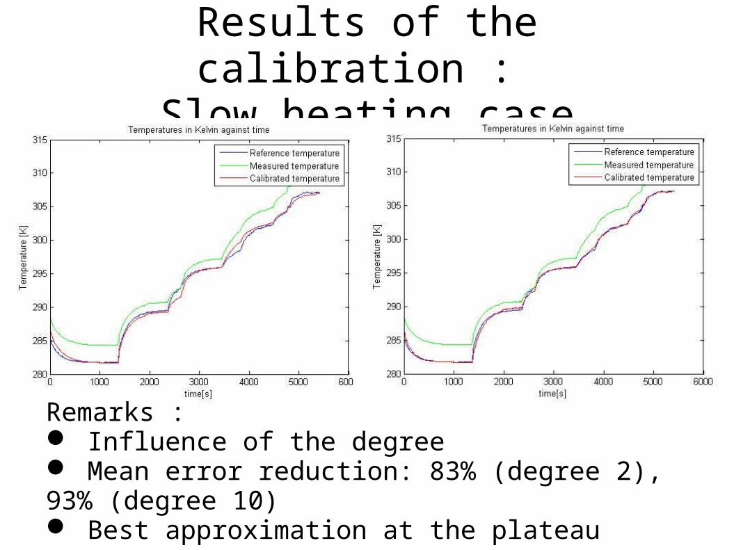
Results of the calibration : Slow heating case

Remarks : Influence of the degree Mean error reduction: 83% (degree 2), 93% (degree 10) Best approximation at the plateau

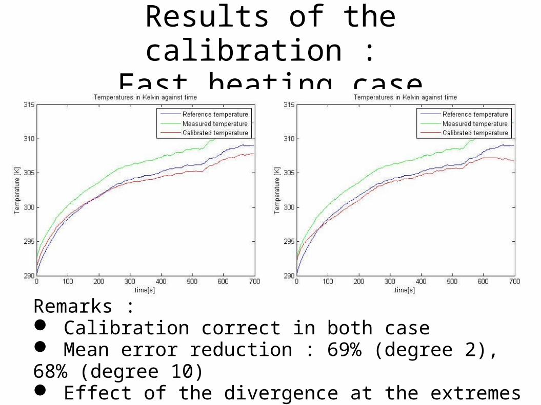
Results of the calibration : Fast heating case

Remarks : Calibration correct in both case Mean error reduction : 69% (degree 2), 68% (degree 10) Effect of the divergence at the extremes

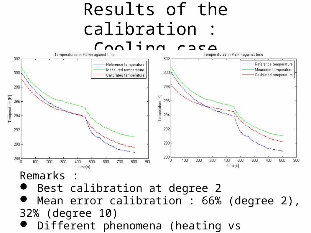
Results of the calibration : Cooling case

Remarks : Best calibration at degree 2 Mean error calibration : 66% (degree 2), 32% (degree 10) Different phenomena (heating vs cooling ?)

Difficulties and observations

The difference of temperature between our sensor and the reference one seems to vary in each experiment for a given temperature.

Example : at 292.5 Kelvin :

ε1═ -0.16 K; ε2═ -1.71 K; ε3═ -2.28 K

Existence of a latency between the real temperature and the measure one ?

Different adaptation time between cooling and heating ?

Difficulties and observations

We don't obtain the same results in the behavior of the curve !

First experiments : the difference between the reference and observed sensors raises at extreme temperature

New experiments : the difference between the reference and observed sensors is smaller at extreme temperature !

Local turbulence ?

Conclusion

The slow heating curve seems to be valid to correct a rising temperature or for non variating temperature.

To improve our calibration, the best is to have the most data as possible and at the largest scale

Choice of the calibration’s degree: depend on what we want

To extrapolate : small degree

To be precise inside the range of obs. temp : high degree

Another experiment ?

Thank you for your attention !

Any questions ?