1

Shunt Calibration for Dummies; a Reference Guide

by

LaVar Clegg

Interface, Inc.Advanced Force Measurement

Scottsdale, Arizona USA

Presented at

Western Regional Strain Gage CommitteeSummer Test and Measurement Conference

August 2, 2005

2

ABSTRACT

Shunt Calibration is a technique for simulating strain in a piezo-resistive strain gage Wheatstone bridge circuit by shunting one leg of the bridge. The bridge may be internal to a discreet transducer or composed of separately applied strain gages. The resulting bridge output is useful for calibrating or scaling instrumentation. Such instrumentation includes digital indicators, amplifiers, signal conditioners, A/D converters, PLC’s, and data acquisition equipment. Care must be taken to understand the circuits and connections, including extension cables, in order to avoid measurement errors.

3

1. What is Shunt Cal ?

• Shunt Calibration = Shunt Cal = SCAL = RCAL

• A means of calibrating or verifying instrumentation by simulating a physical input.

• The simulation is accomplished by shunting one leg of a Wheatstone bridge circuit.

• Not a means of calibrating a transducer.

• A “poor man’s” mV/ V simulator.

4

2. A Good Simulator is Superior to Shunt Cal

• A simulator is not strain sensitive.• Resistor ratios are less temperature sensitive.• Thermal emf errors are minimized by design.• Symmetrical shunting produces less common mode

error.• Provides specific and convenient mV/ V values.• Provides a true zero output.• Has no toggle.• Shunt resistor doesn’t get lost.• A calibration history can be maintained.

5

3. Shunt Cal has some advantages

• Low cost.

• The bridge circuit is already there.

• Need to make and break cable connections can be avoided.

• Can be applied conveniently and at any time and during test programs.

6

4. About Formulae in this Paper

• The formulae herein are derived by the author and he is responsible for any errors.

• Rs = Value of shunt resistor.• Rb = Bridge resistance represented by single value.• Vs = Simulated output at signal leads in units of mV/ V.• Vs is always net (the difference between the shunted

and unshunted readings or similarly the difference between the switch-closed and switch-open readings).

• “ = “ means mathematically exact.• “ “ means close enough for practical purposes.• Infinite input impedance of instrumentation is assumed.

≈

≈

7

4. About Formulae (continued)

• In each circuit type, only one leg of the bridge is shown shunted, for simplicity. But the formulae apply as well to the opposite leg if the resistor numbers are placed in the formula according to position. They also apply to the adjacent legs if resistor numbers are placed according to position and polarity of Vs is reversed.

8

5. Basic Bridge Circuit

Rs

R2

R1

R4

R3

+ Exc

- Exc

- Sig +Sig

21212

21

21000

RRRR

RRRs

RVs++⎟

⎠⎞

⎜⎝⎛ ++

=

9

Simplified Basic Bridge Circuit, R1=R2=Rb

Rs

Rb

Rb

R4

R3

+ Exc

- Exc

- Sig +Sig

5.0

250

+=

RbRs

Vs

10

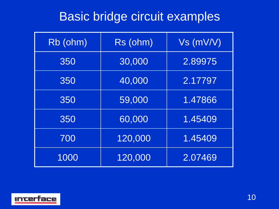
Basic bridge circuit examples

Rb (ohm) Rs (ohm) Vs (mV/V)

350 30,000 2.89975

350 40,000 2.17797

350 59,000 1.47866

350 60,000 1.45409

700 120,000 1.45409

1000 120,000 2.07469

11

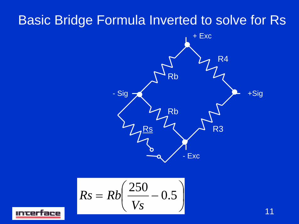
Basic Bridge Formula Inverted to solve for Rs

Rs

Rb

Rb

R4

R3

+ Exc

- Exc

- Sig +Sig

⎟⎠⎞

⎜⎝⎛ −= 5.0250

VsRbRs

12

Basic circuit inverted formula examples

Rb (ohm) Vs (mV/V) Rs (ohm)

350 1 87,325

350 2 43,575

350 3 28,992

700 2 87,150

700 3 57,983

1000 3 82,833

13

R5

Rb

RbRb

Rb

R6

Rs

+ Exc

-Exc

-Sig

6. Bridge With Series Trim or Compensation Resistors

⎟⎠⎞

⎜⎝⎛

++−

+⎟⎠⎞

⎜⎝⎛ +−

+≈

RbRRRR

RsRR

RbRs

Vs56

5614

5615.0

250

+Sig

14

⎟⎠⎞

⎜⎝⎛

++−

+⎟⎠⎞

⎜⎝⎛ +−

+≈

RbRRRR

RsRR

RbRs

V56

5614

5615.0

250

Nominal term

Summationterm

Difference term

This formula for the series resistors case is interesting because it shows that if R5 = R6, Vs is nearly the same as if R5 = R6 = 0. This fact allows a batch of transducers with variations in natural loaded outputs to be trimmed with series resistors to a standard output and all will have a similar Vs.

15

Series resistor circuit examples

Rb (ohm) Rs (ohm) R5 (ohm) R6 (ohm) Vs (mV/V)

350 60,000

60,000

60,000

60,000

60,000

60,000

60,000

0 1.45409

350

0

50

0

50

175

0

50 1.45349

350 50 1.63551

350 0 1.27207

350 175 1.45198

700 100 3.26086

700 100 200 3.18574

16

7. Bridge With Parallel Trim or Compensation Resistor

727215.0

250

RRs

RRb

RbRs

Vs+⎟

⎠⎞

⎜⎝⎛ +⎟⎠⎞

⎜⎝⎛ +

=

+Exc

-Exc

+Sig- Sig

Rb

Rb

Rb

Rb

R7

Rs

17

Parallel resistor circuit examples

Rb (ohm) R7 (ohm) Rs (ohm) Vs (mV/V)

350 4100,000

10,000

1,000

350

350

60,000 1.45409

350 60,000 1.44903

350 60,000 1.40499

350 60,000 1.07751

350 60,000 0.72758

350 30,000 1.45198

18

8. How Does Tolerance of Rb and of Rs affect Vs ?

To a close approximation for all of the circuits above with reasonable values,

• Vs is proportional to the value of Rb and

• Vs is inversely proportional to the value of Rs.

19

9. What Errors are Contributed by Extension Cables ?

It often happens that initial shunt calibration data is recorded on a particular bridge and then in subsequent tests an extension cable has been added between the bridge and the instrument with Rs located at the instrument. It is useful to know the resulting error.

In the following discussion Rc represents the resistance of one conductor of a cable made of multiple similar conductors.

20

Error contributed by a 4-conductor extension

cable

• Error is due primarily to currentflow in –Sig lead.

• Vs error = 500 Rc / Rs (in units of mV/V).

• Error is always same polarity as Vs.

Rb

Rb

Rb

Rb

Rc

Rc

Rc Rc

Rs

+Exc

-Exc

+Sig-Sig

21

4-Conductor Error Examples

Based on 10 ft cable length

Conductor Gauge

Rc(ohm)

Rb(ohm)

Rs(ohm)

Nom Vs(mV/V)

Vs Error(mV/V)

Vs Error(%Vs)

22 0.16 350 30,000 2.8998 0.0027 +0.09

22 0.16 350 60,000 1.4541 0.0013 +0.09

28 0.65 350 60,000 1.4541 0.0054 +0.37

30 1.03 350 60,000 1.4541 0.0086 +0.59

30 1.03 700 60,000 2.8998 0.0086 +0.30

30 1.03 700 120,000 1.4541 0.0043 +0.30

22

Caution !

If Vs is being converted to physical units, remember that the 4-conductor extension cable

changes output of the circuit by the factor

RcRbRb

2+

If Rc is not accounted for in the conversion, the error compounds the Vs error, doubling

it as a % of reading !

23

10. What Error is Contributed by a6-ConductorExtension Cable ?

Rb

Rb

RbRb

Rs

Rc

Rc

Rc

Rc

Rc

Rc

-Sig+Sig

+Exc+Sense

-Sense -Exc

• Same error in Vs as for 4-conductor extension cable.• No error in physical load output due to Rc in Exc leads.• Remote sensing of excitation is the benefit of a

6-conductor cable.

24

11. What Error is Contributed by a7-ConductorExtension Cable ?

Rb

Rb

Rb

Rb

Rc

Rc

Rc

Rc

Rc

Rc

Rc

Rs

+Sense +Exc

+Sig

-Sense -Exc

-Sig

• Only error is Rc adding to Rs for total shunt =Rs+Rc.• Error is negligible for all practical purposes.

25

12. Why are 8-Conductor Cables Sometimes Used ?

• To allow shunt connection to either –Sig or + Sig and have negligible error.

• 7-Conductor and 8-Conductor cables solve the extension cable error problem.

26

13. What Error in Shunt Cal is Caused by a Physical Load ?

• Analyze by assuming a fully active basic bridge circuit.• r = change in gage resistance due to strain.• Error in Vs is proportional to r / Rb.

+Sig-Sig

+Exc

Rs

Rb-r

Rb-rRb+r

Rb+r

-Exc

27

Error due to Physical Loads, Examples(Assuming all legs equally active)

ErrorRb(ohm)

Rs(ohm)

Vs without load

(mV/V) (mV/V) %

1.45409

1.45409

1.45409

1.45409

1.45409

2.89975

350 60,000 0 0 1.45409 0 0

350 60,000 +1 0.35 1.45264 -0.00146 -0.10

350 60,000 +2 0.70 1.45118 -0.00291 -0.20

350 60,000 -2 -0.70 1.45699 +0.00290 +0.20

350 60,000 -1 -0.35 1.45554 +0.00145 +0.10

700 60,000 -1 -0.70 2.90265 +0.00290 +0.10

PhysicalLoad

(mV/V)

r(ohm)

Vs withload

(mV/V)

Generalized Rule: For any Rb and Rs, Error in % = - 0.1 X Physical Load in mV/V

28

14. What is the Effect on Shunt Cal of a Permanent Zero Balance Shift ?

• If all legs are equally active and somewhat equally shifted in resistance, as is often the case with a mild physical overload, error in Vs follows the same analysis as in paragraph 13 above.

• It is wise to assume that any significant permanent zero shift invalidates a prior Shunt Cal.

29

15. What is the Effect on Shunt Cal of Transducer Toggle ?

• Toggle is a reversible change in bridge zero resulting from the most recent loading changing from tension to compression or vice versa.

• The error in Vs follows the same analysis as in paragraph 13 above.

• Toggle seldom exceeds 0.01 mV/V even for load excursions as high as +/- 4 mV/V.

• Therefore error in Vs seldom exceeds 0.001% for any Rb or Rs.

• The error is normally negligible.

30

16. Is There Reason to Prefer Any Particular Leg of the Bridge to Shunt ?

• Probably not.

• In terms of stability and repeatability, all legs are contributing equally to a shunt measurement.

• R5 and R6 contribute equally to Vs for shunt measurement on any leg regardless of their values. Remember paragraph 6 !

⎟⎠⎞

⎜⎝⎛

++−

+⎟⎠⎞

⎜⎝⎛ +−

+≈

RbRRRR

RsRR

RbRs

Vs56

5614

5615.0

250

31

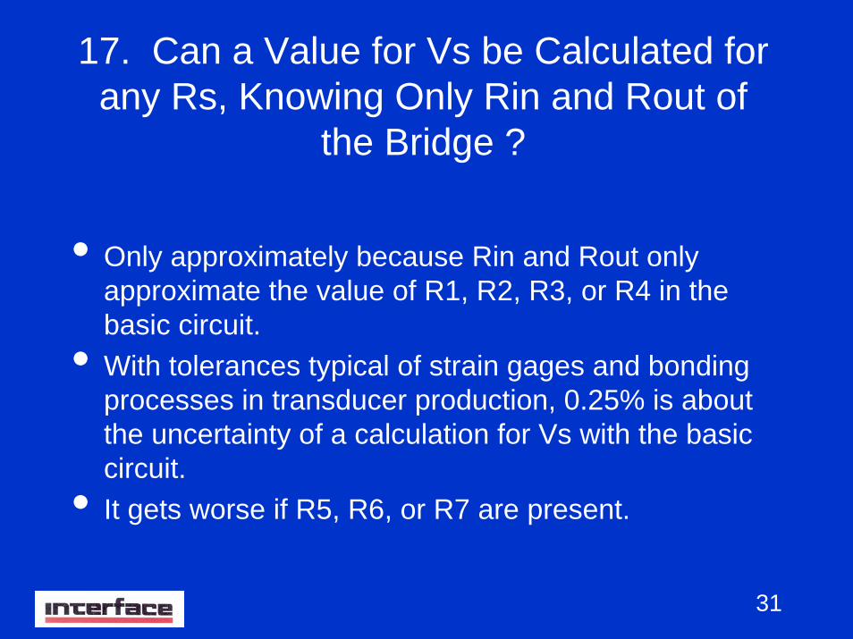
17. Can a Value for Vs be Calculated for any Rs, Knowing Only Rin and Rout of

the Bridge ?

• Only approximately because Rin and Rout only approximate the value of R1, R2, R3, or R4 in the basic circuit.

• With tolerances typical of strain gages and bonding processes in transducer production, 0.25% is about the uncertainty of a calculation for Vs with the basic circuit.

• It gets worse if R5, R6, or R7 are present.

32

18. Where May the Shunt Resistor Be Located ?

a. Internal to a transducer or permanently wired to a bridge circuit.

• Resistor tolerance not important.• Resistor should have low temperature coefficient of

resistance (TCR).

33

b. Internal to an Instrument.

• Low resistor tolerance is important unless a bridge and specific instrument are always used together.

• TCR should be low.

9840HRBSC

These high end instruments have 0.01% Low TCR Internal Shunt Cal Resistors in two different values. Instruments may be substituted without significant error.

34

9830

9820

These lower cost instruments have 1% tolerance Shunt Cal Resistors. For good Vs measurements, instruments should not be substituted.

35

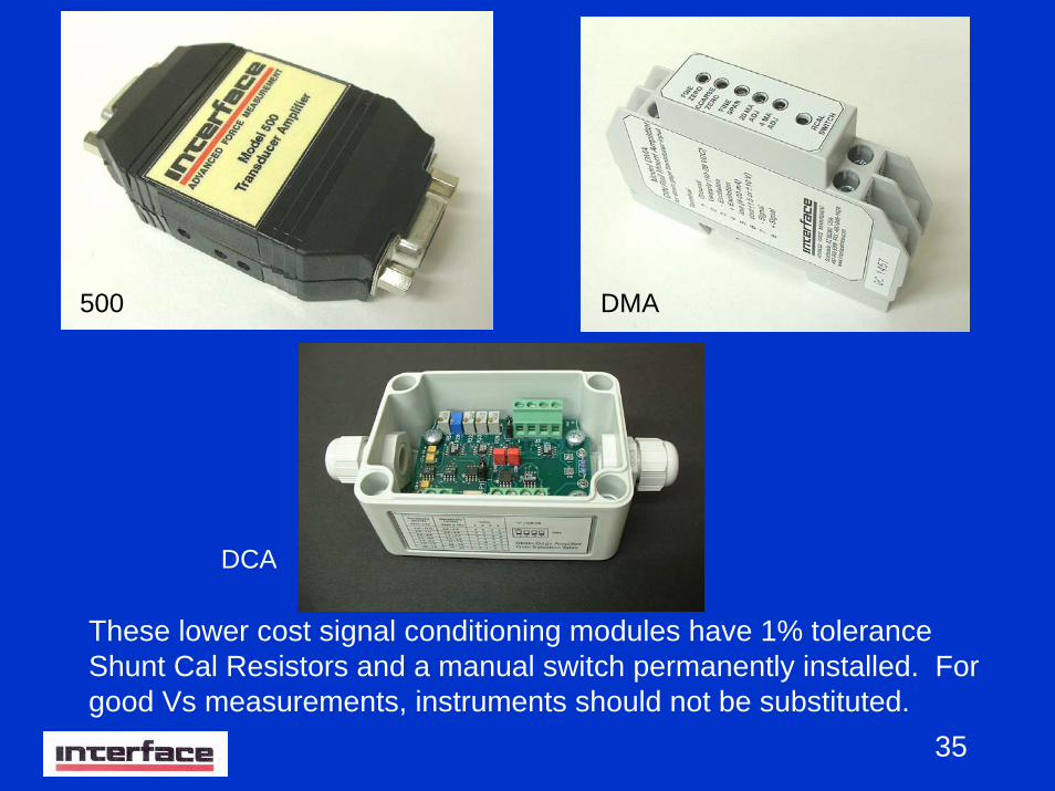
500 DMA

DCA

These lower cost signal conditioning modules have 1% tolerance Shunt Cal Resistors and a manual switch permanently installed. For good Vs measurements, instruments should not be substituted.

36

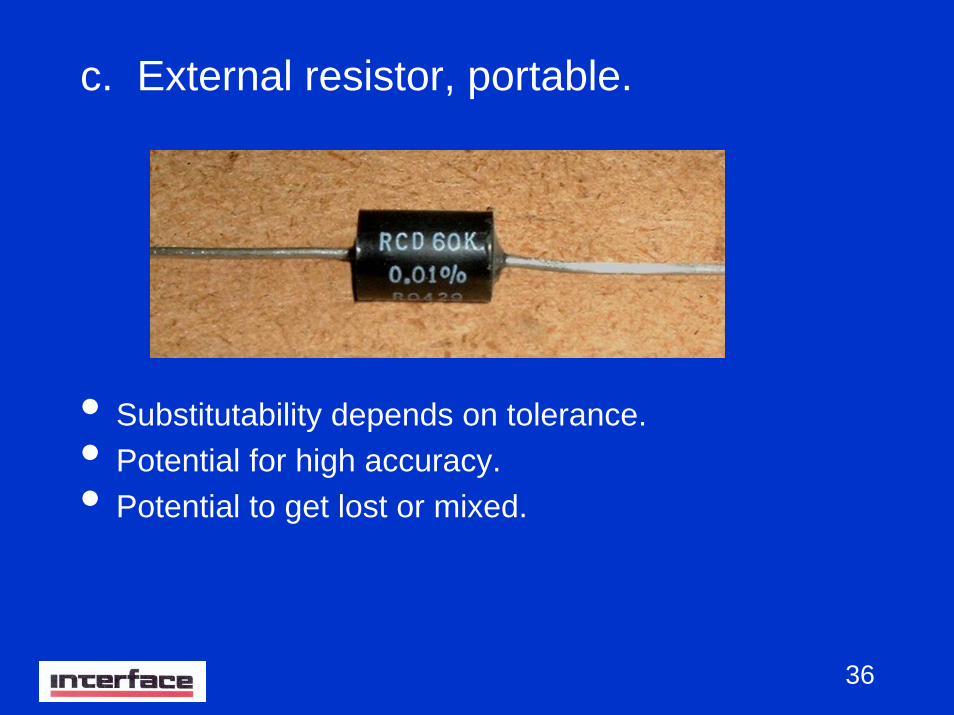
c. External resistor, portable.

• Substitutability depends on tolerance.• Potential for high accuracy.• Potential to get lost or mixed.

37

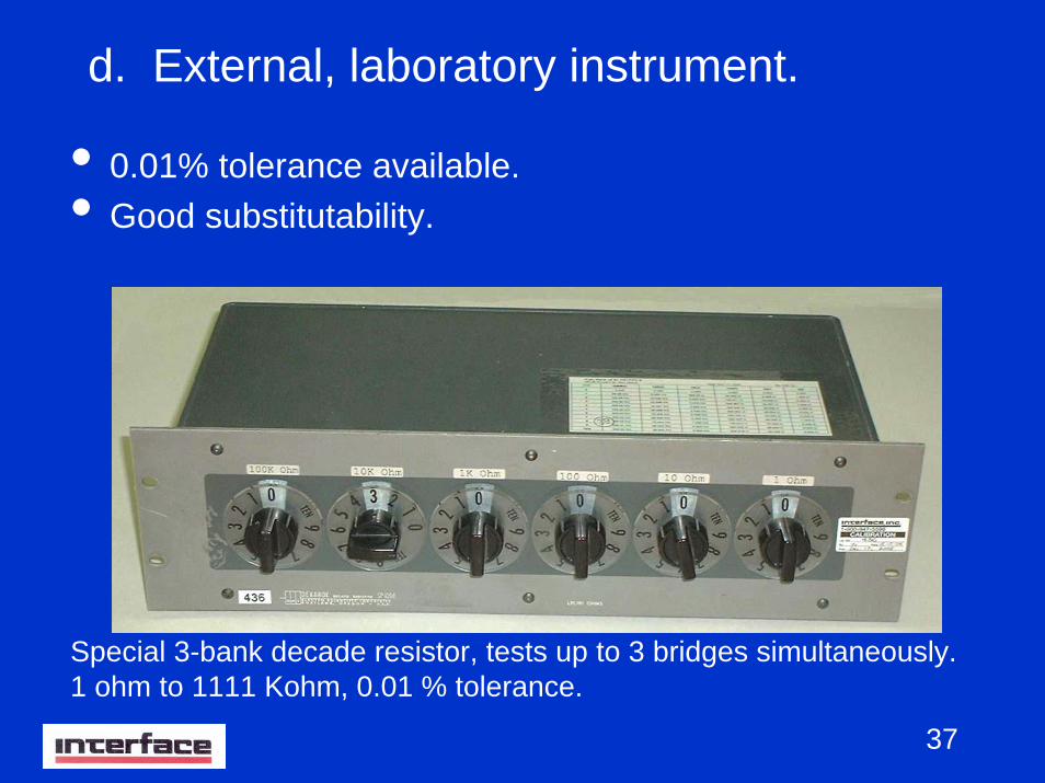
d. External, laboratory instrument.

• 0.01% tolerance available.• Good substitutability.

Special 3-bank decade resistor, tests up to 3 bridges simultaneously. 1 ohm to 1111 Kohm, 0.01 % tolerance.

38

19. What Shunt Cal Repeatability Can Be Expected From Modern Transducers ?

Procedure for a repeatability test performed• 100 Klbf Load Cell specimen loaded in compression. • 12 test cycles of 4 mV/V hydraulically applied physical load and 1

mV/V Shunt Cal on two bridge legs.• Rb = 350 ohm, Rs = 88750 ohm, 20 ppm/°C, internal to load cell.• Measurements over 3 days.• Interface Gold Standard HRBSC instrumentation.

Results of test • Std Dev of physical load measurement: 0.004%.• Std Dev of Shunt Cal: 0.001% pos, 0.001% neg.

39

Shunt Calibration Repeatability Data "

Model: 1232BKN-100KS/N: 103014 Bridge A Internal Shunt Resistor: 88.75 KohmStandards usedSTD-16,BRD4,BRD1

Sequence 1 2 3 4 5 6 7 8 9 10 11 12 Std Dev .Date 3-26-1999, 3-26-1999, 3-26-1999, 3-26-1999, 3-26-1999, 3-26-1999, 3-26-1999, 3-26-1999, 3-26-1999, 3-26-1999, 3-29-1999, 3-29-1999, Time 16:44:11 16:51:29 16:56:25 17:01:10 17:11:22 17:17:24 18:03:14 18:08:02 20:33:34 20:37:16 07:28:39 07:33:36Temp F 75 75 75 75 75 75 75 75 75 75 75 75Humidity % 32 32 32 32 32 32 32 32 32 32 32 32Load mode COMPR COMPR COMPR COMPR COMPR COMPR COMPR COMPR COMPR COMPR COMPR COMPRUnits Klbf Klbf Klbf Klbf Klbf Klbf Klbf Klbf Klbf Klbf Klbf Klbf

LOAD (Klbf):0 -0.01424 -0.01429 -0.01429 -0.01432 -0.01433 -0.01436 -0.01340 -0.01343 -0.01333 -0.01341 -0.01331 -0.01342

20 -0.81384 -0.81388 -0.81394 -0.81402 -0.81406 -0.81403 -0.81302 -0.81309 -0.81303 -0.81305 -0.81293 -0.8130640 -1.61358 -1.61367 -1.61370 -1.61382 -1.61385 -1.61385 -1.61283 -1.61283 -1.61280 -1.61286 -1.61271 -1.6128760 -2.41373 -2.41383 -2.41380 -2.41390 -2.41392 -2.41390 -2.41297 -2.41294 -2.41284 -2.41296 -2.41271 -2.4128480 -3.21476 -3.21483 -3.21484 -3.21486 -3.21486 -3.21483 -3.21399 -3.21403 -3.21392 -3.21395 -3.21365 -3.21373

100 -4.01617 -4.01619 -4.01616 -4.01620 -4.01613 -4.01609 -4.01558 -4.01549 -4.01537 -4.01530 -4.01510 -4.0150540 -1.61607 -1.61617 -1.61616 -1.61619 -1.61613 -1.61603 -1.61555 -1.61555 -1.61542 -1.61540 -1.61520 -1.615200 -0.01413 -0.01416 -0.01415 -0.01418 -0.01421 -0.01421 -0.01332 -0.01334 -0.01329 -0.01332 -0.01327 -0.01332

Span (mV/'V) -4.00193 -4.00190 -4.00187 -4.00188 -4.00180 -4.00173 -4.00218 -4.00206 -4.00204 -4.00189 -4.00179 -4.00163 0.00014 mV/VSHUNT CAL (mV/V) -0.004 %Raw zero -0.01429 -0.01426 -0.01428 -0.01429 -0.01434 -0.01434 -0.01340 -0.01344 -0.01346 -0.01345 -0.01339 -0.01343Raw Neg SCAL -0.99896 -0.99894 -0.99897 -0.99898 -0.99901 -0.99904 -0.99810 -0.99812 -0.99814 -0.99812 -0.99807 -0.99810Net Neg SCAL -0.98467 -0.98468 -0.98469 -0.98469 -0.98467 -0.98470 -0.98470 -0.98468 -0.98468 -0.98467 -0.98468 -0.98467 0.00001 mV/V% Dev from avg -0.001 0.000 0.001 0.001 -0.001 0.002 0.002 0.000 0.000 -0.001 0.000 -0.001 -0.001 %

Raw zero -0.01428 -0.01428 -0.01430 -0.01432 -0.01433 -0.01434 -0.01343 -0.01344 -0.01346 -0.01347 -0.01341 -0.01347Raw Pos SCAL 0.97123 0.97125 0.97123 0.97122 0.97118 0.97118 0.97210 0.97206 0.97207 0.97204 0.97210 0.97205Net Pos SCAL 0.98551 0.98553 0.98553 0.98554 0.98551 0.98552 0.98553 0.98550 0.98553 0.98551 0.98551 0.98552 0.00001 mV/V% Dev from avg -0.001 0.001 0.001 0.002 -0.001 0.000 0.001 -0.002 0.001 -0.001 -0.001 0.000 0.001 %