Sam Houston State University

Department of Economics and International Business Working Paper Series

________________________________________________________

Inequality and Economic Growth Over the Business Cycle: Evidence From U.S. State-Level Data

Mark W. Frank, Donald G. Freeman

SHSU Economics & Intl. Business Working Paper No. SHSU_ECO_WP03-01 July 2003

Abstract: The purpose of this paper is to re-examine the empirical relationship between income inequality and economic growth using U.S. State-level data during the post-war period. The use of state-level data provides a sample that is relatively homogeneous in many non-economic characteristics, unlike the international data used in most previous work. Building upon prior research, this study addresses the issues of potential non-linearities in the relationship between inequality and growth, the influence of the cyclical condition during the year sampled, and possible bias in the measurement of economic growth. We find, using GMM estimators, that inequality is harmful to growth, and that the deleterious effects of inequality are greater for lower income states.

SHSU ECONOMICS WORKING PAPER

1

Inequality and Economic Growth Over the Business Cycle: Evidence From U.S. State-Level Data

by

Mark W. Frank, Ph.D.Department of Economics and International Business

Sam Houston State UniversityP.O. Box 2118

Huntsville, TX 77341-2118tel. (936) 294-4890fax. (936) 294-3488

E-mail: markfrank@shsu.edu

and

Donald G. Freeman, Ph.D.Department of Economics and International Business

Sam Houston State UniversityP.O. Box 2118

Huntsville, TX 77341-2118tel. (936) 294-1264fax. (936) 294-3488

E-mail: eco_dgf@shsu.edu

2

Inequality and Economic Growth Over the Business Cycle: Evidence From U.S. State-Level Data

Abstract

The purpose of this paper is to re-examine the empirical relationship between income inequality

and economic growth using U.S. State-level data during the post-war period. The use of state-level

data provides a sample that is relatively homogeneous in many non-economic characteristics, unlike the

international data used in most previous work. Building upon prior research, this study addresses the

issues of potential non-linearities in the relationship between inequality and growth, the influence of the

cyclical condition during the year sampled, and possible bias in the measurement of economic growth.

We find, using GMM estimators, that inequality is harmful to growth, and that the deleterious effects of

inequality are greater for lower income states.

I. Introduction

There is now a large and growing literature, both theoretical and empirical, examining the

relationship between income inequality and economic growth. Early on, this relationship was usually

assumed to be negative. Galor and Zeira (1993), also Aghion and Bolton (1997), argue that credit

market imperfections limit the ability of low-income individuals to invest in human capital, leaving

productivity gains unexploited. The political economy models of Alesina and Rodrik (1994) and

Persson and Tabellini (1994) stress the efficiency losses from re-distributional schemes and government

intervention as median voters use the political system to flatten the income distribution. Gupta (1990)

3

and Alesina and Perotti (1996) emphasize the potential for social unrest and political upheaval from

increased inequality and the consequent diversion of resources toward social control. Empirical

evidence, primarily cross-country regressions of economic growth over long periods on inequality and

other control variables, tended to support the negative view. Bénabou (1996) provides a useful survey

of much of this literature.

Over time, however, an alternate view of the inequality-growth nexus developed, with

researchers emphasizing the positive aspects of inequality for growth. In one variation of this view,

inequality may reflect more flexible labor markets that bring about higher levels of work effort and

entrepreneurial energy leading to stronger economic growth (Metzler, 1998; Siebert, 1998). Separately,

Galor and Tsiddon (1997) develop a model in which technological shocks concentrate productivity

growth and factor payments in the advancing sectors of the economy. Barro (2000) proposes that

because political power follows from economic power, concentration of income can lead to government

policies favoring economic growth. Some recent empirical work tends to support these alternative

views, with positive relationships between growth and inequality found by Forbes (2000) for a panel of

countries, and Partridge (1997) for a panel of U.S. states.

Still other empirical work, however, notably by Barro (2000), Quah (2001), and Panizza (2002)

find little or no stable relationship between inequality and growth; results appear to be extremely sensitive

to econometric specification or data set (Deininger and Squire, 1998; Barro, 2000). In general then, the

evolution of the empirical literature on inequality and growth has moved from finding mainly negative

relationships, to finding some positive relationships, to finding little or no relationship. The ambiguity is

unfortunate, because inequality is clearly increasing, at least in the U.S., and whether and by how much

4

this change in inequality is associated with a change in economic performance is an important question.

[Figure 1 about here]

Figure 1 illustrates changes in two measures of income distribution for U.S. households for the

period 1967-2001. The top line (left scale) shows the ratio of the 95th percentile income limit to the 20th

percentile income limit. In 2001, the income of the household at the 95th percentile ($150,499) was 8.4

times the income of the household at the 20th percentile ($17,970), the high for the time range. Similarly,

the Gini coefficient1, an inequality measure encompassing the entire income distribution, has increased by

25 percent since its low in 1968. Current levels of inequality are unprecedented in the post-war period,

and represent a clear reversal of the decline in inequality experienced by U.S. families prior to the

1970s.

However, one must be cautious in attempting to infer relationships from aggregate U.S. data.

Aggregate growth in the U.S. has been influenced by any number of factors during the past 50 years,

and any attempt to partial out the effect of changes in income inequality is vulnerable to the problems of

multicollinearity among the regressors, and the potential endogeneity of inequality itself. For these

reasons, we use pooled U.S. state-level data, which offers enhanced variability, additional controls for

heterogeneity, and a methodology to address endogeneity issues, as discussed below.

The greater homogeneity of U.S. states vis-a-vis international panels mitigates the difficulty in

adequately capturing the structural differences across the latter group confronted by earlier studies such

as Forbes (2000). Corruption levels, labor market flexibility, tax neutrality, tradition of entrepreneurship,

and many other factors are only poorly measured, if at all, and these sources of heterogeneity are much

more likely to contribute to omitted variable bias across countries than across U.S. states. Therefore,

5

estimation using U.S. state-level data is more likely to accurately estimate the ceteris paribus effect of a

change in inequality on the change in economic growth

These data have been explored before, notably by Partridge (1997) and Panizza (2002).

Partridge (1997) estimates a panel of 48 states using decennial U.S. Census data with controls for initial

income, education, and industrial structure, finding that initial inequality is positively associated with

subsequent 10-year cumulative growth in state income. These results were among the first empirical

findings that challenged the view that inequality was harmful for economic growth. Panizza (2002),

however, using income data from tax returns, “concludes that, at the U.S. cross-state level, there is no

clear, robust relationship between inequality and growth and that small differences in the method used to

measure income inequality and in the econometric specification yield substantial differences in the

estimated relationship between inequality and growth.” (P. 25) Empirically, therefore, the relationship

between inequality and economic growth at the U.S. state level appears to remain an open question.

The purpose of this paper is to re-examine the U.S. state-level inequality/growth nexus by

employing three new approaches to the data. First, following Barro (2000), we recognize inherent non-

linearities in the data, which neither Partridge (1997) nor Panizza (2002) do.2 In a previous paper

(Frank and Freeman, 2002), we showed that the effect of inequality on growth was negative, and more

pronounced at lower levels of income. Second, we use Internal Revenue Service data, which are

available on an annual basis, to control for the possible influence of the business cycle. There is some

evidence that inequality is counter cyclical (Johnson and Shipp, 1999), and results using decennial data in

prior studies may be biased by omitting the cyclical condition of the economy during the sample year.

We provide regressions using decade- based data and using the peak years of business cycles during the

6

post-war period to control for cyclical effects. As we show, the choice of the sample years has a

material effect on the results.

Third, we employ an alternative measure of economic growth as our dependent variable in some

regressions. The focus on per capita (i.e., mean) income growth in previous studies may not reflect the

effect of inequality on the typical individual’s income, which is arguably better measured by median

income in a distribution as skewed as that in the U.S. Clearly, incomes can be increasing rapidly at the

top level of the income distribution but nowhere else, leading to increases in inequality and average

incomes, but leaving the bulk of the population no better off.3 Our principal finding is that in a variety

of specifications, time periods, and data sources, initial income inequality is negatively related to

subsequent economic growth at the state level. This negative relationship is statistically significant in most

models, especially those in which inequality is treated as endogenous to the system. Our results thus

stand in contrast to the positive relationship found by Partridge (1997) and Forbes (2000), and unlike

those of Panizza (2002), are robust to different specifications. In the preponderance of cases, we also

find that the negative relationship is stronger at lower income levels, although this result is not as clear-cut

using the IRS data.

The paper is organized as follows. Section II describes the data and provides some descriptive

statistics. Section III presents the empirical results, and Section IV concludes.

II Data and Methodology

The model that we estimate is based on the conditional growth equation of Barro (1991) or

Mankiw, Romer and Weil (1992). Growth ending in period t is a function of the initial level of income

7

and other conditioning factors, including the distribution of income, all measured at the beginning of the

period, or t-1:

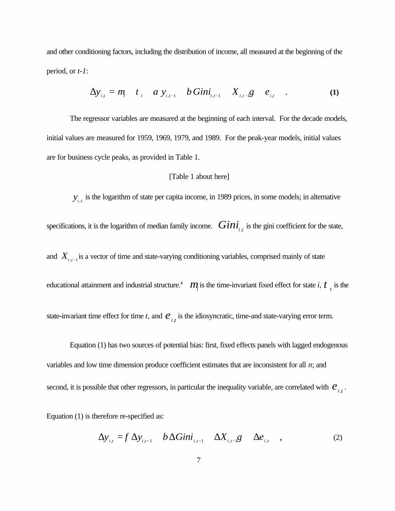
∆y y Gini Xi t i t i t i t i t i t, , , , , .= + + + + +− − −µ τ α β γ ε1 1 1 (1)

The regressor variables are measured at the beginning of each interval. For the decade models,

initial values are measured for 1959, 1969, 1979, and 1989. For the peak-year models, initial values

are for business cycle peaks, as provided in Table 1.

[Table 1 about here]

is the logarithm of state per capita income, in 1989 prices, in some models; in alternativeyi t,

specifications, it is the logarithm of median family income. is the gini coefficient for the state,Ginii t,

and is a vector of time and state-varying conditioning variables, comprised mainly of stateXi t, −1

educational attainment and industrial structure.4 is the time-invariant fixed effect for state i, is theµi τ t

state-invariant time effect for time t, and is the idiosyncratic, time-and state-varying error term. ε i t,

Equation (1) has two sources of potential bias: first, fixed effects panels with lagged endogenous

variables and low time dimension produce coefficient estimates that are inconsistent for all n; and

second, it is possible that other regressors, in particular the inequality variable, are correlated with . ε i t,

Equation (1) is therefore re-specified as:

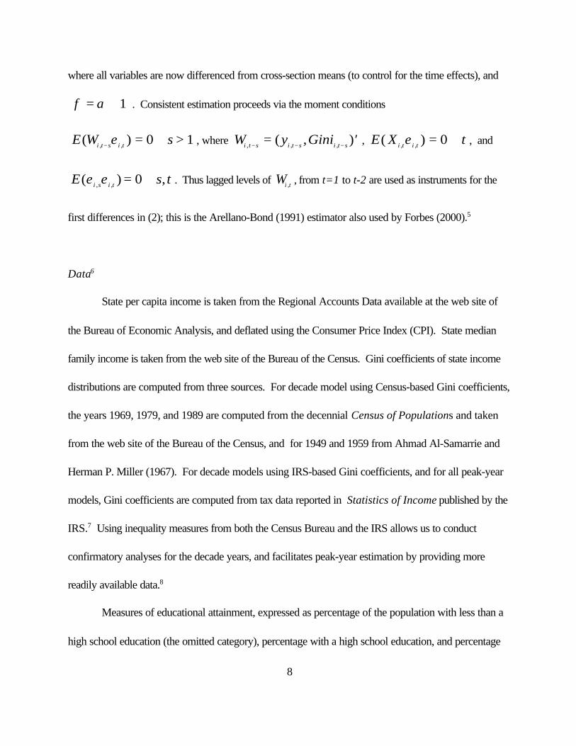
∆ ∆ ∆ ∆ ∆y y Gini Xi t i t i t i t i t, , , , , ,= + + +− − −φ β γ ε1 1 1 (2)

8

where all variables are now differenced from cross-section means (to control for the time effects), and

. Consistent estimation proceeds via the moment conditionsφ α= + 1

, where , , andE W si t s i t( ), ,− = ∀ >ε 0 1 W y Ginii t s i t s i t s, , ,( , )− − −= ′ E X ti t i t( ), ,ε = ∀0

. Thus lagged levels of , from t=1 to t-2 are used as instruments for theE s ti s i t( ) ,, ,ε ε = ∀0 Wi t,

first differences in (2); this is the Arellano-Bond (1991) estimator also used by Forbes (2000).5

Data6

State per capita income is taken from the Regional Accounts Data available at the web site of

the Bureau of Economic Analysis, and deflated using the Consumer Price Index (CPI). State median

family income is taken from the web site of the Bureau of the Census. Gini coefficients of state income

distributions are computed from three sources. For decade model using Census-based Gini coefficients,

the years 1969, 1979, and 1989 are computed from the decennial Census of Populations and taken

from the web site of the Bureau of the Census, and for 1949 and 1959 from Ahmad Al-Samarrie and

Herman P. Miller (1967). For decade models using IRS-based Gini coefficients, and for all peak-year

models, Gini coefficients are computed from tax data reported in Statistics of Income published by the

IRS.7 Using inequality measures from both the Census Bureau and the IRS allows us to conduct

confirmatory analyses for the decade years, and facilitates peak-year estimation by providing more

readily available data.8

Measures of educational attainment, expressed as percentage of the population with less than a

high school education (the omitted category), percentage with a high school education, and percentage

9

with at least a bachelor’s degree are also computed from the decennial Census of Populations and

taken from the web site of the Bureau of the Census. Industrial structure is measured as the percent of

wage and salary income by industry category, and is taken from the Regional Accounts Data available at

the web site of the Bureau of Economic Analysis.

In some specifications, we allow for non-linearity in the inequality/income relation by including an

interaction term, the product of the gini coefficient and the level of income, a procedure also used by

Barro (2000). The inclusion of this term strengthens the principle conclusions, provides further evidence

of omitted variable bias in previous work, and permits an interesting interpretation of the results.

Sample data for estimation for the decade years are collected in 10 year intervals, spanning from

1959 to 1999. Because the dependent variable is the growth rate of the 10-year interval following the

observation on the independent variables, the independent variables span 1959 to 1989, while the

dependent variable spans 1959 to 1999. The number of states used is 48.9 This brings the number of

observations to 192 for the first-differenced GMM estimations of equation (2). Data for the peak years

are constructed in a similar manner; the dependent variable is the state per capita income growth rate for

the business cycle following the peak year. With nine business cycles during the period 1945-2001 (the

short cycle from 1/80 to 7/81 is ignored), there are 432 observations available for the peak year model.

The means and standard deviations of the variables are reported in Table 2, below.

III Empirical Results

Table 2 reports the means and standard deviations of the variables used in this study, together

with Ordinary Least Squares (OLS) fixed effects estimates of Equation (1), above. The OLS estimates

10

treat all regressors as at least predetermined, and as stated above, are known to be inconsistent. They

are presented here to provide a baseline for the GMM estimates to follow below.

[Table 2 about here]

The OLS models employ the parsimonious specification favored by Forbes (2000), which

includes only educational structure as control variables (the remaining variables, for which means and

standard deviations are provided, will be used in the GMM estimates). We find that inequality is

negatively and significantly related to economic growth at the state level, for either measure of the Gini

coefficient. In the business cycle peak model, which uses the IRS Gini exclusively, inequality is also

negatively and significantly related to economic growth. The coefficient of the initial level of income is

negative in all specifications, consistent with the convergence hypothesis, which posits that with

diminishing returns to capital and free exchange of technology, economies with lower initial incomes will

experience faster growth. The educational variables are positive and usually significant, as expected; a

higher level of initial education leads to stronger economic growth.

In Table 3, we address the issue of potential endogeneity of the explanatory variables by

employing the GMM estimation of Equation (2) for the decade models. These estimates are

comparable to those of Partridge (1997), Forbes (2000), and Panizza (2002). As noted, time and

fixed effects are eliminated via the differencing process, but the estimator continues to be a within

estimator that controls for aggregate changes over time, like modifications to the national tax code or

changes in macroeconomic policy. As in Table 2, what is being measured by the coefficients is the

change in economic growth within a state to a change in inequality (or to changes in the other

explanatory variables), not the differences in economic growth across states.

11

In columns (1) and (4), inequality is treated as an exogenous variable; in columns (2) and (3), (5)

and (6), the Gini coefficient is instrumented as described above. In columns (3) and (6), interaction

terms are introduced to test for potential non-linearity in the response of growth to inequality. Again, we

report results for both Census and IRS Gini coefficients, both as a test of the robustness of our results,

and to establish the comparability of the IRS Gini for the models employing the peak year data, below.

The results of models (1) and (4) are broadly similar, with the exception of the coefficient of the

initial income level, which is not significant in the IRS model. As in Table 2, inequality is negatively and

significantly related to economic growth, but the coefficient is much smaller than the estimates in Table 2.

The education variables continue to be positively related to growth. Specification tests on models (1)

and (4) are not encouraging, however. Arellano and Bond (AB) (1991) suggest a test of second-degree

autocorrelation of the residuals of the GMM estimates; rejection of the test indicates that the assumption

of lagged levels of the regressors as valid instruments is untenable. In models (1) and (4), the null of no

second degree autocorrelation is rejected. The two-step Sargan test is a check of the over-identifying

restrictions; a rejection of the null indicates that the residuals are correlated with the instrumental

variables. In models (1) and (4), the null of Sargan test is also rejected, so we proceed to estimation

with the Gini coefficient treated as an endogenous variable.

In models (2) and (5), the patterns of the coefficients are quite similar to (1) and (4), but the

magnitude of the coefficient of the inequality variable is about three times larger. The coefficient for the

college-educated proportion of the population remains significant, but that for the high school not so.

The failure to reject the AB test of autocorrelation is an improvement, but the Sargan test indicates that

some specification error remains. Possible causes include omitted variables or non-linearity in the

12

relationship, both of which are addressed in the specifications to follow.

Models (3) and (6) include interaction terms between inequality and initial levels of income,

similar to specifications estimated by Barro (2000). The general idea is that inequality may have different

effects depending on the level of economic development. In both models, the interaction terms are

positive, indicating that the negative effect of inequality on growth is greater for lower-income states;

Barro (2000) finds similar results for a panel of countries. The transformation and differencing of the

variables make direct interpretation of the coefficients difficult, but the range of effects in model (3) of a

change in the Gini coefficient from its minimum value in 1999 (0.371) to its maximum value (0.466) is a

change in the average ten-year state economic growth of between -0.60 to -0.04 per cent, or -0.38 on

average, compared to the +2.23 mean ten-year state economic growth rate over the sample.10 As

Barro notes, the lesser effect of inequality at higher income levels may stem from the better developed

credit markets and the greater degree of income mobility at higher levels of development.

As noted, the rejection of the Sargan test suggests the continued existence of some sort of

specification error, even in the non-linear model. We therefore attempt to address this issue by

incorporating controls for structural change in the economic activity of the states, an approach also used

by Partridge (1997). As economic growth is partly the explained by technological change, and if

increased inequality is associated with technological change, as suggested by Galor and Tsiddon (1997),

the omission of changing economic structure from the model potentially biases the coefficients of the

inequality variables.

Table 4 reports the results of the decade models with interaction terms extended to include the

percentage of state wage and salary income by industry (farming is the omitted category). Four models

13

are reported, corresponding to the two Gini measures, and for two measures of income, per capita, as in

the previous Tables, and median income. As noted above, given the skewness of income distributions,

median income may provide a better measure for the “representative” individual.

[Table 4 about here]

What we actually find is that the inclusion of the industry employment shares in the per capita

income models changes the principal results very little; the coefficients on the inequality variables are

reduced somewhat, as they should be if the technological change connection is there, and the educational

coefficients are also reduced. The coefficients of the industry share variables tend to show that those

states who are further along in making the transition from goods-producing to service producing

economies have experienced faster growth, but this conclusion is very tentative.

The use of median income growth as a dependent variable also makes very little difference in the

estimated outcomes, producing almost no change in the census Gini models in columns (1) and (2), and

very little change (and none of significance in the variables of interest) in the IRS Gini models in (3) and

(4). What we do see, however, is some improvement in the Sargan test, especially in columns (1) and

(4), suggesting that the inclusion of the structural change variables does mitigate somewhat the possibility

of omitted variable bias.

Testing the effects of the business cycle on the growth/inequality nexus

The use of Census Gini coefficients for state-level income distributions has restricted previous

analyses to decade years prior to the decennial census, placing limits on the number of available

observations and possibly confounding the estimates by placing the observations at different points in the

14

business cycle. To address these issues, we have calculated Gini coefficients for all the peak years of

the business cycles experienced since World War II, as listed in Table 1, using grouped data from

individual income tax returns, as reported annually by the IRS in the publication Statistics of Income.11

These data were also used by Panizza (2002). The advantage of using IRS data is the potential gain in

accuracy from the large number of tax returns available, versus the Census method of relying on

sampling (and the usual issues of survey responses); the disadvantage is in the large number of income

earners who are not required to file tax returns, as well as those who are recipients of non-cash or non-

reportable forms of income.

Table 5 reports the results of alternative estimates of equation (2) similar to the previous results

for the decade years. We note that the number of observations more than doubles, adding to greater

precision of the estimated coefficients. We find that the principal conclusions of the decade models are

maintained by using business cycle peak years, with the notable exception that the interaction term in

columns (3) and (4) is below the Census interaction term seen previously (see Tables 3 and 4), but

above the IRS interaction term. By contrast, the coefficient on the Gini variable is about half the size as

previously. We also find that the education coefficients are much smaller and statistically insignificant in

the peak year estimations. One very positive outcome is that the AB test of autocorrelation and the

Sargan test indicate that the increased number of observations and the use of peak year data indicate

that the instrument set is valid.

IV Conclusions

Although the results obtained so far are intriguing, there is far more to do before we are able to

15

draw any firm conclusions regarding the relationship between inequality and economic growth at the

U.S. state level. The extensions to the existing analysis that are contemplated include conducting

sensitivity analyses with tests of coefficient stability over time. There is some evidence that the

relationship between income growth and inequality is weaker during the early part of the sample period

than in the later part.

Also, the moment conditions that we are relying on to achieve consistent estimation are

questionable if, for example, the underlying factors explaining both inequality and income growth persist

over time (which is reasonable). Therefore, the use of identifying instruments outside the set of lagged

values of existing regressors would be a valuable test of the robustness of the relationship, as would the

use of a panel VAR to exploit the potential feedback mechanism between inequality and growth and

better understand the direction of causality between them. We are hopeful that the development of an

annual data set using the IRS data will allow us to achieve this result.

Finally, the variables we have chosen to measure inequality and economic performance are

traditional but by no means exhaustive. The use of different measures of inequality, including income

shares and Lorenz ordinates, and the use of different measures of economic performance, including

Gross State Product and employment growth as alternative dependent variables would provide more

comprehensive tests of the growth/inequality nexus.

16

References

Alesina, A. and R. Perotti, 1996. “Income Distribution, Political Instability and Investment,” European

Economic Review, 81, 5, 1170-1189.

Alesina, A. and D. Rodrik, 1994. “Distribution Politics and Economic Growth,” Quarterly Journal of

Economics, 109, 465-490.

Arellano, M. and S. Bond, 1991. “Some Tests of Specification for Panel Data: Monte Carlo Evidence

and an Application to Employment Equations,” Review of Economic Studies 58, 277-97.

Al-Samarrie, A. and H. Miller, 1967. “State Differentials in Income Concentration,” American

Economic Review 57, 59-72.

Andrews, D. and B. Lu, 2001. “Consistent Model and Moment Selection Procedures for GMM

Estimation with Application to Dynamic Panel Data Models,” Journal of Econometrics 101,

123-164.

Atkinson, A.B. and A Brandolini, 2001. “Promise and Pitfalls in the Use of ‘Secondary’ Data-Sets:

Income Inequality in OECD Countries as a Case Study,” Journal of Economic Literature, 39,

771-799.

Barro, R., 2000. “Inequality and Growth in a Panel of Countries,” Journal of Economic Growth, 5, 5-

32.

Barro, R. 1991. “Economic Growth in a Cross-Section of Countries,” Quarterly Journal of

Economics, 106, 407-444.

Bénabou, R., 1996. “Inequality and Growth,” NBER Working Paper 5658.

17

Deninger, K and L. Squire, 1996. “A New Data Set Measuring Income Inequality,” World Bank

Economic Review, 10, 565-591.

Forbes, K., 2000. “A Reassessment of the Relationship Between Inequality and Growth,” American

Economic Review, 90, 869-887.

Frank, M.W. and D.G. Freeman, 2002. “Relationship of Inequality to Economic Growth: Evidence from

U.S. State-Level Data,” Pennsylvania Economic Review, 11, 24-36.

Galor, O. and D. Tsiddon, 1997. “The Distribution of Human Capital and Economic Growth,” Journal

of Economic Growth, 2, 93-124.

Galor, O. and J. Zeira, 1993. “Income Distribution and Macroeconomics,” Review of Economic

Studies, 60, 35-52.

Gottschalk, P., and T. Smeeding, (1997). “Cross-national Comparisons of Earnings and Income

Inequality,” Journal of Economic Literature, 35, 633-687.

Gupta, D., 1990. The Economics of Political Violence, New York, Prager.

Johnson, D.S. and S Shipp, 1999. “Inequality and the Business Cycle: A Consumption Viewpoint,”

Empirical Economics, 24, 173-180.

Kakwani, N.C., 1980. Income Inequality and Poverty: Methods of estimation and Policy

Applications, New York, Oxford University Press for the World bank.

Kuznets, S., 1955. “Economic Growth and Income Inequality,” American Economic Review, 45, 1-

28.

Mankiw, G., D. Romer and D. Weil, 1992. “A Contribution to the Empirics of Economic Growth,”

Quarterly Journal of Economics, 107, 407-437.

18

McCloskey, D. and S. Ziliak, 1996. “The Standard Error of Regression,” Journal of Economic

Literature, 34, 97-114.

Meltzer, A., 1998. “Discussion on ‘Economic Consequences of Income Inequality,’ ” in Income

Inequality: Issues and Policy Options. A Symposium Sponsored by the Federal Reserve

Bank of Kansas City. Kansas City, KS, Federal Reserve Bank of Kansas City.

Panizza, U., 2002. “Income Inequality and Economic Growth: Evidence from American Data,” Journal

of Economic Growth, 7, 25-41.

Partridge, M., 1997. “Is Inequality Harmful for Growth? Comment,” American Economic Review, 87,

1019-1032.

Persson, T. and G. Tabellini, 1994. “Is Inequality Harmful for Growth? Theory and Evidence,”

American Economic Review, 84, 600-621.

Quah, D., 2001. “Some Simple Arithmetic on How Income Inequality and Economic Growth Matter,”

LSE Economics Working Paper.

Saint-Paul, G. and T. Verdler, 1993. “Education, Democracy, and Growth,” Journal of Development

Economics, 42, 2, 399-407.

Sala-I-Martin, X., 1996. “The Classical Approach to Convergence Analysis,” Economic Journal, 106,

1019-36.

Siebert, H., 1998. “Comment on ‘Economic Consequences of Income Inequality,’ ” in Income

Inequality: Issues and Policy Options. A Symposium Sponsored by the Federal Reserve

Bank of Kansas City. Kansas City, KS, Federal Reserve Bank of Kansas City.

19

1. There are many possible interpretations of the Gini coefficient (see Kakwani, 1980), but perhaps themost common is the Gini coefficient as one minus twice the area under the Lorenz curve, the latter beingthe plot of the cumulative proportion of income received against the cumulative proportion of incomeunits, arranged in ascending order of income.

2. Of course, the famous Kuznets (1955) curve between the level of income and income inequality ishighly nonlinear.

3.Indeed, in the U.S., inflation-adjusted incomes for the top 5 per cent of the population increased by96 percent, and for those in the top 20 percent by 59 percent during the period 1980-2001. Incomesin the bottom 40 per cent increased by 12 per cent during the same period.

4.These are the principle controls used by Partridge (1997); Forbes (2000) uses only educationalattainment and inflation for her main results.

5.It is possible to specify other moment conditions for (2), depending on whether individual regressorsare endogenous, predetermined, or strictly exogenous, and whether the fixed effects are correlated withthe regressors; see Donald W. K. Andrews and Biao Lu (2001). Because the tradeoff is betweenefficiency (if the moment conditions are correct) and inconsistency (if they are not), we have chosen tolimit the conditions to the Arellano and Bond (1991) conditions used by KF.

6.The data used in this paper are available as an Excel worksheet from the authors on request.

7.The Internal Revenue Service Gini coefficients are calculated using data on the number of returns andthe adjusted gross income (before taxes) by state and by size of the adjusted gross income. Thisdistributional data is available annually from various publications by the Internal Revenue Service. Forthe years 1945 to 1981, the data is available in the Statistics of Income, Individual Income Tax Returnsannual series. For the years 1982 to 1987, the data series was not published but is available by requestfrom the Internal Revenue Service. For the years 1988 to 2001, the data is available in the Statistics ofIncome Bulletin quarterly series.

8.The correlation between IRS and Census Gini indexes for the sample period is 0.52. Whileseemingly small, it is higher than the 0.44 found by Panizza (2002) for similar data, or the 0.48 betweenthe estimates for OECD country data of Deininger and Squire (1996) and Gottschalk and Smeeding(1997). Panizza (2002) suggests that the censoring of the IRS data at the low end of the distributionmay explain the difference, but topcoding procedures for the Census data may also contribute.

Notes

20

9.Ahmad Al-Samarrie and Herman P. Miller (1967) do not compute gini coefficients for Alaska orHawaii; data are available for Washington, D.C., but the high proportion of commuters to residentsmakes it a special case.

10.The example chosen is an extreme; a change of 0.1 in the Gini coefficient represents about 5standard deviations. The mean of a one standard deviation change in inequality would therefore beabout a -0.07 percent change in average growth.

11.In a future project, we plan to calculate Gini coefficients (and other measures of income inequality)on an annual basis in order to conduct time series analysis of the research questions addressed in thispaper.

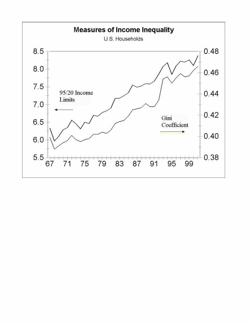
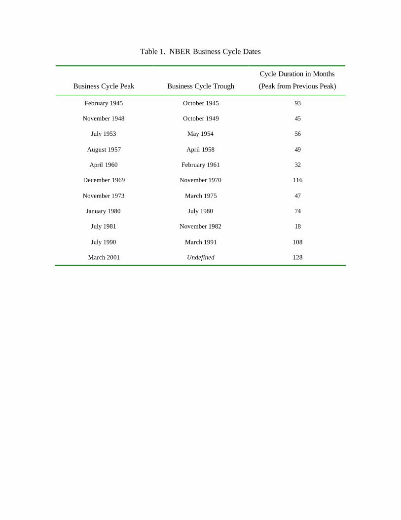
Table 1. NBER Business Cycle Dates

Business Cycle Peak

Business Cycle Trough

Cycle Duration in Months

(Peak from Previous Peak)

February 1945 October 1945 93

November 1948 October 1949 45

July 1953 May 1954 56

August 1957 April 1958 49

April 1960 February 1961 32

December 1969 November 1970 116

November 1973 March 1975 47

January 1980 July 1980 74

July 1981 November 1982 18

July 1990 March 1991 108

March 2001 Undefined 128

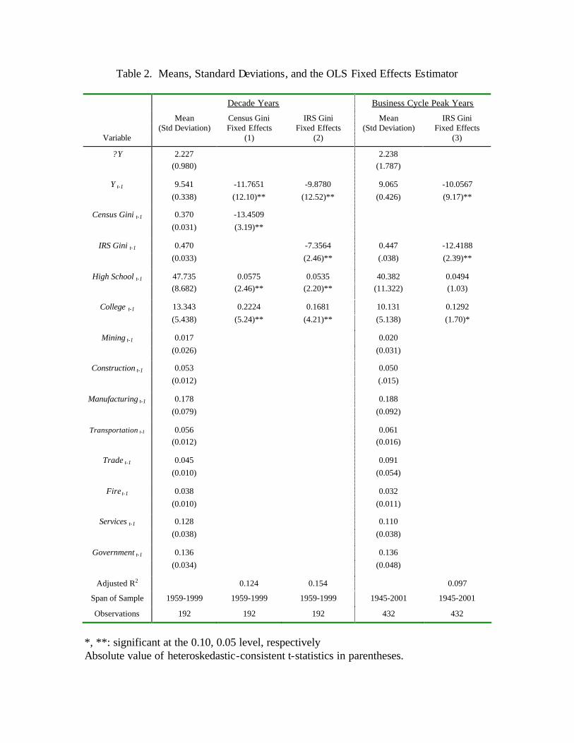
Table 2. Means, Standard Deviations, and the OLS Fixed Effects Estimator

Decade Years Business Cycle Peak Years

Mean Census Gini IRS Gini Mean IRS Gini (Std Deviation) Fixed Effects Fixed Effects (Std Deviation) Fixed Effects

Variable (1) (2) (3)

?Y 2.227 2.238 (0.980) (1.787)

Y t-1 9.541 -11.7651 -9.8780 9.065 -10.0567 (0.338) (12.10)** (12.52)** (0.426) (9.17)**

Census Gini t-1 0.370 -13.4509 (0.031) (3.19)**

IRS Gini t-1 0.470 -7.3564 0.447 -12.4188 (0.033) (2.46)** (.038) (2.39)**

High School t-1 47.735 0.0575 0.0535 40.382 0.0494 (8.682) (2.46)** (2.20)** (11.322) (1.03)

College t-1 13.343 0.2224 0.1681 10.131 0.1292 (5.438) (5.24)** (4.21)** (5.138) (1.70)*

Mining t-1 0.017 0.020 (0.026) (0.031)

Construction t-1 0.053 0.050 (0.012) (.015)

Manufacturing t-1 0.178 0.188 (0.079) (0.092)

Transportation t-1 0.056 0.061 (0.012) (0.016)

Trade t-1 0.045 0.091 (0.010) (0.054)

Fire t-1 0.038 0.032 (0.010) (0.011)

Services t-1 0.128 0.110 (0.038) (0.038)

Government t-1 0.136 0.136 (0.034) (0.048)

Adjusted R2 0.124 0.154 0.097

Span of Sample 1959-1999 1959-1999 1959-1999 1945-2001 1945-2001

Observations 192 192 192 432 432

*, **: significant at the 0.10, 0.05 level, respectively Absolute value of heteroskedastic-consistent t-statistics in parentheses.

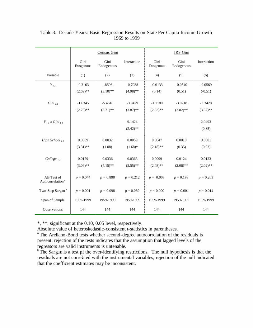
Table 3. Decade Years: Basic Regression Results on State Per Capita Income Growth, 1969 to 1999

Census Gini IRS Gini

Gini Exogenous

Gini Endogenous

Interaction Gini Exogenous

Gini Endogenous

Interaction

Variable (1) (2) (3) (4) (5) (6)

Y t-1 -0.3163 -.8606 -0.7938 -0.0133 -0.0540 -0.0569

(2.69)** (3.10)** (4.98)** (0.14) (0.51) (-0.51)

Gini t-1 -1.6345 -5.4618 -3.9429 -1.1189 -3.0218 -3.3428

(2.70)** (3.71)** (3.87)** (2.53)** (3.82)** (3.52)**

Y t-1 x Gini t-1 9.1424 2.0493

(2.42)** (0.35)

High School t-1 0.0069 0.0032 0.0059 0.0047 0.0010 0.0001

(3.31)** (1.08) (1.68)* (2.18)** (0.35) (0.03)

College t-1 0.0179 0.0336 0.0363 0.0099 0.0124 0.0123

(3.06)** (4.15)** (5.55)** (2.03)** (2.06)** (2.02)**

AB Test of Autocorrelation a

p = 0.044 p = 0.890 p = 0.212 p = 0.008 p = 0.193 p = 0.203

Two-Step Sargan b p = 0.001 p = 0.098 p = 0.089 p = 0.000 p = 0.001 p = 0.014

Span of Sample 1959-1999 1959-1999 1959-1999 1959-1999 1959-1999 1959-1999

Observations 144 144 144 144 144 144

*, **: significant at the 0.10, 0.05 level, respectively. Absolute value of heteroskedastic-consistent t-statistics in parentheses. a The Arellano-Bond tests whether second-degree autocorrelation of the residuals is present; rejection of the tests indicates that the assumption that lagged levels of the regressors are valid instruments is untenable. b The Sargan is a test pf the over-identifying restrictions. The null hypothesis is that the residuals are not correlated with the instrumental variables; rejection of the null indicated that the coefficient estimates may be inconsistent.

Table 4. Decade Years: Extended Regression Results on State Per Capita and Median Income Growth, 1969 to 1999

Census Gini IRS Gin i

Per Capita Median Per Capita Median

Variable (1) (2) (3) (4)

Y t-1 -0.2365 -0.4866 0.3850 0.3194 (1.03) (2.07)** (2.69)** (2.24)**

Gini t-1 -3.4373 -3.4418 -2.3054 -2.8433 (3.35)** (3.04)** (2.54)** (2.87)**

Y t-1 x Gini t-1 7.2381 6.9159 0.6849 -3.6028 (1.82)* (1.79)* (0.17) (1.24)

High School t-1 0.0034 0.0006 0.6849 -0.0041 (1.06) (0.25) (0.31) (1.39)

College t-1 0.0292 0.0279 0.0096 0.0108 (4.38)** (3.73)** (1.65)* (1.76)*

Mining t-1 -1.3064 -0.8945 -0.8257 -0.7653 (2.78)** (2.01)** (2.09)** (1.07)

Construction t-1 -3.0704 -1.5689 -2.8293 -2.1265 (3.23)** (2.10)** (2.97)** (2.20)**

Manufacturing t-1 -1.0368 -0.7528 -0.4451 -0.4924 (3.09)** (2.09)** (1.33) (1.52)

Transportation t-1 -2.0168 -0.5242 0.8520 0.7584 (1.23) (0.31) (0.73) (0.53)

Trade t-1 0.8577 1.3399 1.5892 2.0982 (0.76) (1.30) (1.05) (1.28)

Fire t-1 -1.1168 -1.2120 0.0184 -1.7602 (0.46) (0.65) (0.01) (0.83)

Services t-1 0.1730 0.1510 -0.0597 -0.0809 (0.18) (0.15) (0.07) (0.09)

Government t-1 -0.0821 -0.0198 1.1398 0.9193 (0.14) (0.03) (1.62) (1.59)

AB Test of Autocorrelation p = 0.251 P = 0.309 p = 0.297 p = 0.155

Two-Step Sargan p = 0.162 P = 0.051 p = 0.040 p = 0.101

Span of Sample 1959-1999 1959-1999 1959-1999 1959-1999

Observations 144 144 144 144

*, **: significant at the 0.10, 0.05 level, respectively. Absolute value of heteroskedastic-consistent t-statistics in parentheses. Also, see notes for Tables 3.

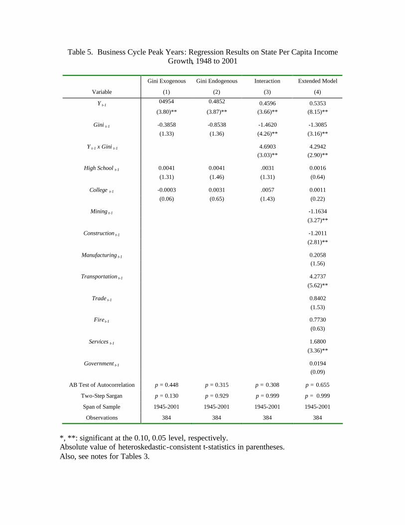
Table 5. Business Cycle Peak Years: Regression Results on State Per Capita Income Growth, 1948 to 2001

Gini Exogenous Gini Endogenous Interaction Extended Model

Variable (1) (2) (3) (4)

Y t-1 04954 0.4852 0.4596 0.5353 (3.80)** (3.87)** (3.66)** (8.15)**

Gini t-1 -0.3858 -0.8538 -1.4620 -1.3085 (1.33) (1.36) (4.26)** (3.16)**

Y t-1 x Gini t-1 4.6903 4.2942 (3.03)** (2.90)**

High School t-1 0.0041 0.0041 .0031 0.0016 (1.31) (1.46) (1.31) (0.64)

College t-1 -0.0003 0.0031 .0057 0.0011 (0.06) (0.65) (1.43) (0.22)

Mining t-1 -1.1634 (3.27)**

Construction t-1 -1.2011 (2.81)**

Manufacturing t-1 0.2058 (1.56)

Transportation t-1 4.2737 (5.62)**

Trade t-1 0.8402 (1.53)

Fire t-1 0.7730 (0.63)

Services t-1 1.6800 (3.36)**

Government t-1 0.0194 (0.09)

AB Test of Autocorrelation p = 0.448 p = 0.315 p = 0.308 p = 0.655

Two-Step Sargan p = 0.130 p = 0.929 p = 0.999 p = 0.999

Span of Sample 1945-2001 1945-2001 1945-2001 1945-2001

Observations 384 384 384 384

*, **: significant at the 0.10, 0.05 level, respectively. Absolute value of heteroskedastic-consistent t-statistics in parentheses. Also, see notes for Tables 3.