
Shrinkage in Empirical Bayes Estimates for Diagnostics … · Division of Pharmacokinetics and Drug...
41
Division of Pharmacokinetics and Drug Therapy Department of Pharmaceutical Biosciences Uppsala University, Uppsala, Sweden Shrinkage in Empirical Bayes Estimates for Diagnostics and Estimation: Problems and Solutions Radojka M. Savić & Mats O. Karlsson
Transcript of Shrinkage in Empirical Bayes Estimates for Diagnostics … · Division of Pharmacokinetics and Drug...

Division of Pharmacokinetics and Drug TherapyDepartment of Pharmaceutical Biosciences
Uppsala University, Uppsala, Sweden
Shrinkage in Empirical Bayes Estimates for Diagnostics and Estimation:
Problems and Solutions
Radojka M. Savić & Mats O. Karlsson

Outline
Empirical Bayes Estimates
Use in Non-linear Mixed Effects Modelling
Shrinkage phenomenon
Shrinkage related problems:
Diagnostics
Estimation process (FOCE & NONP)
Solutions & Recommendations
Empirical Bayes Estimates
POSTHOC estimates – individual parameter estimates
Provide population PKPD modellers with:
EBE - individual parameter estimate IPRED – individual predictions IWRES – individual weighted residuals
IWRESij=(DVij-IPREDij)/SD(εij)
Use of EBEs
Diagnostics • IPRED vs DV• IWRES vs IPRED• EBE vs EBE• EBE vs Covariate• GAM
Estimation • FOCE• Nonparametric estimation
Predicition (TDM) Simulation
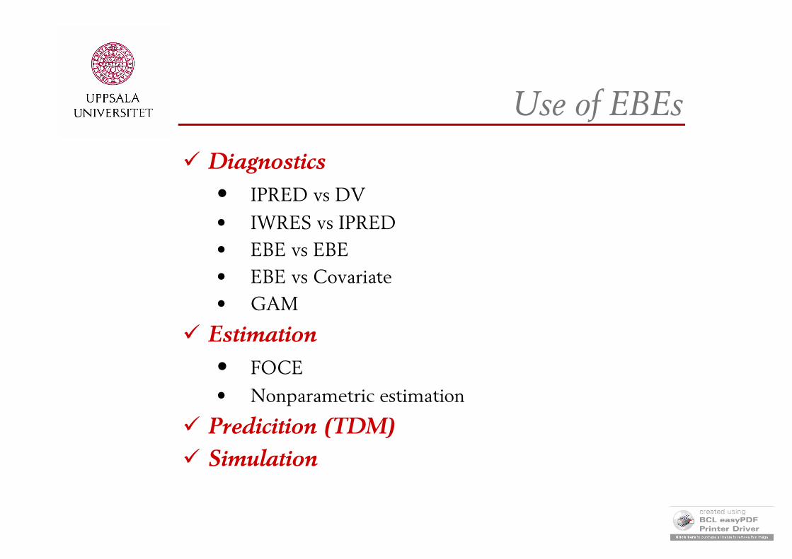
Diagnostics based on EBEs
Increases resolution by separating variability components
If data are uniformative:
1. EBE distribution will shrink towards 0 (population mean)EBE 0
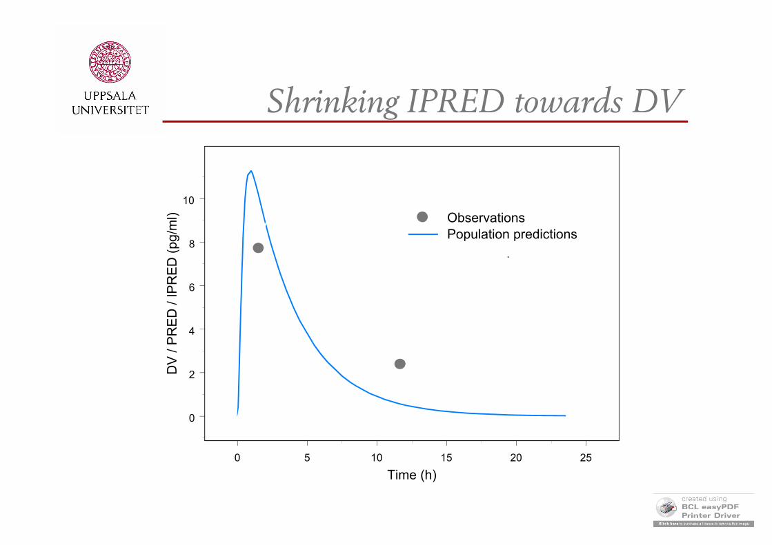
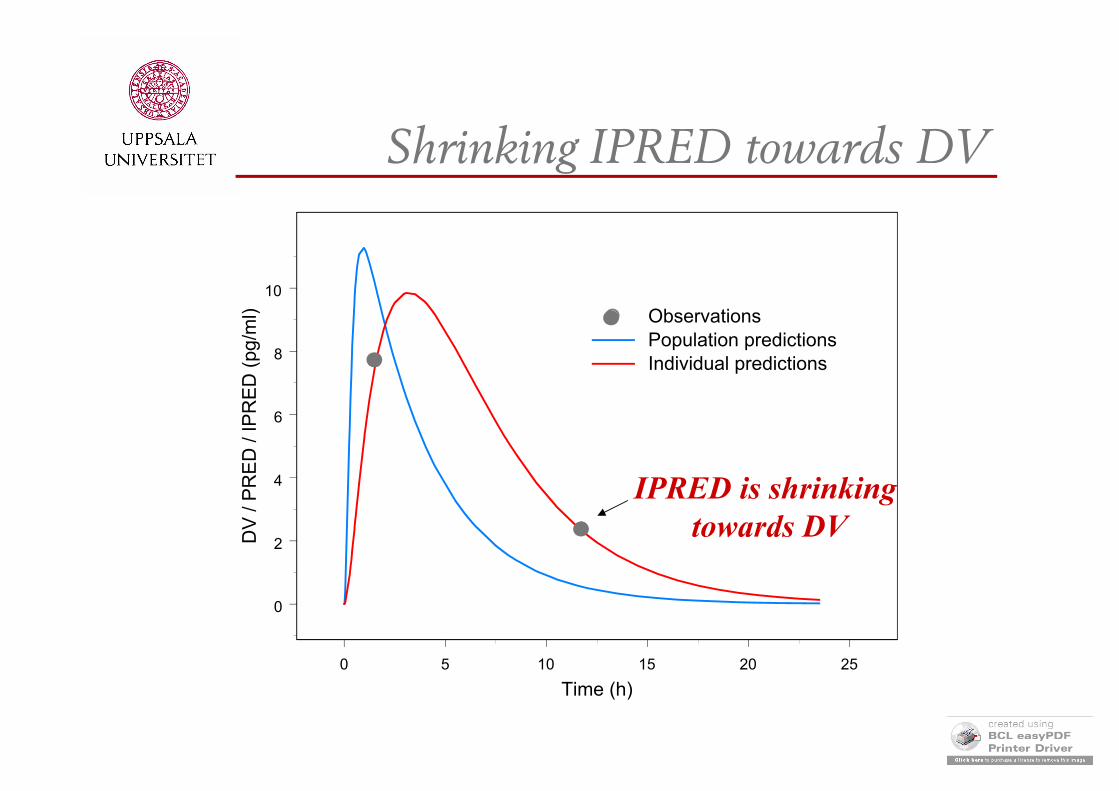
2. Individual predictions (IPRED) will shrink towards the corresponding observation (DV)
IPRED DV
3. IWRES, residual components will shrink towards 0IWRES 0
R.M. Savic, J.J. Wilkins and M.O. Karlsson. (Un)informativeness of EBE-based diagnostics, AAPS J, Abstract T3360, 2006.
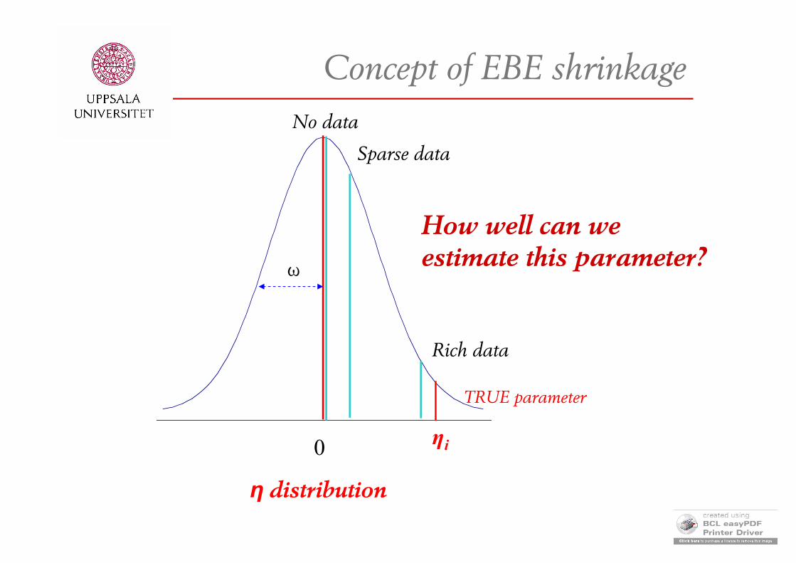
ω
Concept of EBE shrinkage
η distribution
No data
Sparse data
How well can we estimate this parameter?
TRUE parameter
0
Rich data
ηi

Shrinking EBE distribution towards 0
Post Hoc η values
Pro
babi
lity
Den
sity
Fun
ctio
n
Ω decrease
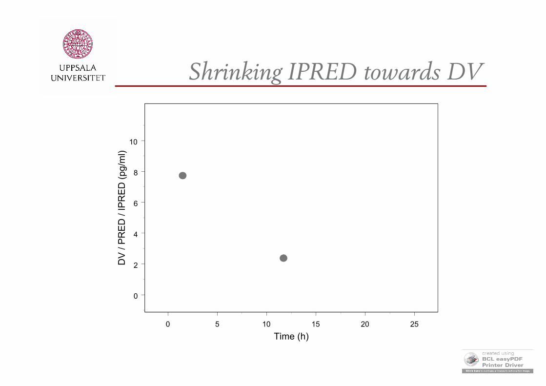
Shrinking IPRED towards DV
0 5 10 15 20 25
Time (h)
0
2
4
6
8
10
DV
/ P
RE
D /
IPR
ED
(pg
/ml) Observations
Population predictionsIndividual predictions
Shrinking IPRED towards DV
0 5 10 15 20 25
Time (h)
0
2
4
6
8
10
DV
/ P
RE
D /
IPR
ED
(pg
/ml) Observations
Population predictionsIndividual predictions
Shrinking IPRED towards DV
0 5 10 15 20 25
Time (h)
0
2
4
6
8
10
DV
/ P
RE
D /
IPR
ED
(pg
/ml) Observations
Population predictionsIndividual predictions
IPRED is shrinking towards DV

Shrinking IWRES towards 0
)(SD
IPREDDVIWRES ijij
ij
If IPRED DV
IWRES 0
IWRES values
Pro
babi
lity
Den
sity
Fun
ctio
n
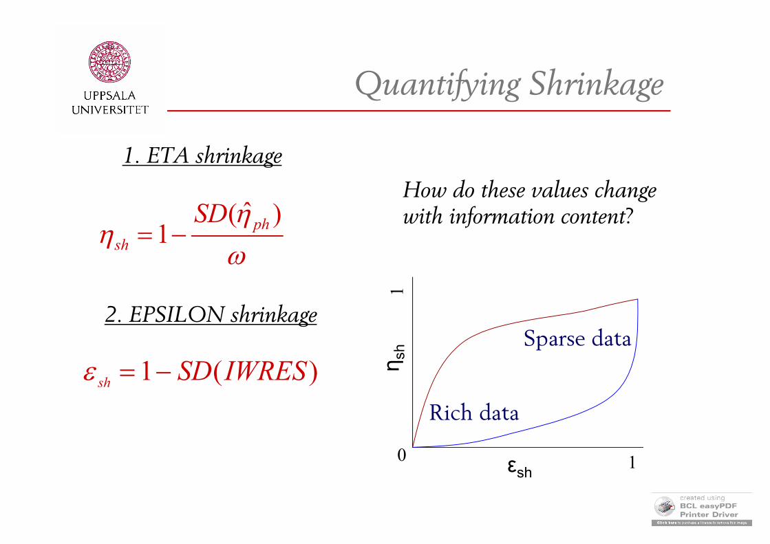
Quantifying Shrinkage
ˆ( )1 ph
sh
SD
εsh
η sh
0 1
1Rich data
Sparse data
How do these values change with information content?
)(1 IWRESSDsh
1. ETA shrinkage
2. EPSILON shrinkage

How shrinkage may influence diagnostics?
Diagnostics explored:
1. EBE-related diagnostics (- shrinkage)• EBE distribution plots• EBE vs EBE plots• EBE vs Covariate plots
2. IPRED / IWRES - related diagnostics (ε - shrinkage)• IPRED vs DV plot• IWRES vs IPRED plot
Methods: MC simulations True model was fitted to data unless otherwise stated Graphical diagnostics showed on single simulation example
to facilitate visualization
-3 -2 -1 0 1 2 3
0.0
0.1
0.2
0.3
0.4
0.5
0.6
Value
Pro
babi
lity
-3 -2 -1 0 1 2 3
0.0
0.1
0.2
0.3
0.4
0.5
0.6
Value
Pro
babi
lity
-3 -2 -1 0 1 2 3
0.0
0.1
0.2
0.3
0.4
0.5
0.6
Value
Pro
babi
lity
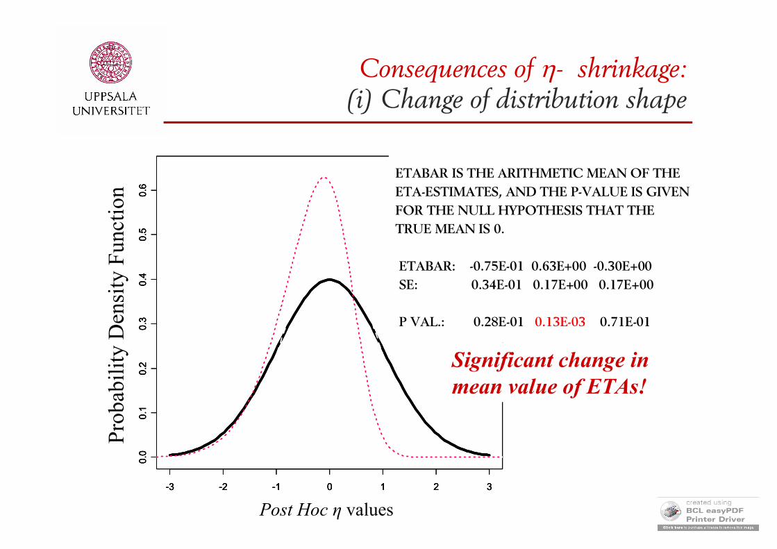
Consequences of - shrinkage:(i) Change of distribution shape
Post Hoc η values
Pro
babi
lity
Den
sity
Fun
ctio
n
ETABAR IS THE ARITHMETIC MEAN OF THEETA-ESTIMATES, AND THE P-VALUE IS GIVENFOR THE NULL HYPOTHESIS THAT THE TRUE MEAN IS 0.
ETABAR: -0.75E-01 0.63E+00 -0.30E+00 SE: 0.34E-01 0.17E+00 0.17E+00
P VAL.: 0.28E-01 0.13E-03 0.71E-01
Significant change in mean value of ETAs!
ETA1
-1.1
-0.6
-0.1
0.4
0.9
-1.0 -0.5 0.0 0.5 1.0
-1.0
-0.5
0.0
0.5
1.0
-1.1 -0.6 -0.1 0.4 0.9
ETA2
ETA1
-1.1
-0.6
-0.1
0.4
0.9
-1.0 -0.5 0.0 0.5 1.0
-1.0
-0.5
0.0
0.5
1.0
-1.1 -0.6 -0.1 0.4 0.9
ETA2
correct shrunk
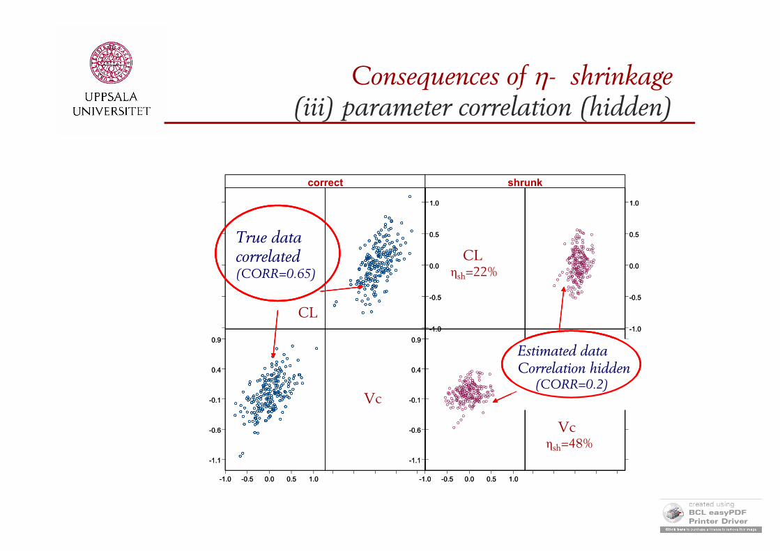
True data correlated(CORR=0.65)
Estimated data Correlation hidden
(CORR=0.2)Vc
Vcηsh=48%
CLηsh=22%
CL
ETA1
-1.1
-0.6
-0.1
0.4
0.9
-1.0 -0.5 0.0 0.5 1.0
-1.0
-0.5
0.0
0.5
1.0
-1.1 -0.6 -0.1 0.4 0.9
ETA2
ETA1
-1.1
-0.6
-0.1
0.4
0.9
-1.0 -0.5 0.0 0.5 1.0
-1.0
-0.5
0.0
0.5
1.0
-1.1 -0.6 -0.1 0.4 0.9
ETA2
correct shrunk
True data correlated(CORR=0.65)
True data correlated(CORR=0.65)
Estimated data Correlation hidden
(CORR=0.2)
Estimated data Correlation hidden
(CORR=0.2)Vc
Vcηsh=48%
CLηsh=22%
CL
Consequences of - shrinkage(iii) parameter correlation (hidden)
CL
-1.1
-0.6
-0.1
0.4
0.9
-1.0 -0.5 -0.0 0.5 1.0
-1.0
-0.5
-0.0
0.5
1.0
-1.1 -0.6 -0.1 0.4 0.9
V
CL
-1.1
-0.6
-0.1
0.4
0.9
-1.0 -0.5 -0.0 0.5 1.0
-1.0
-0.5
-0.0
0.5
1.0
-1.1 -0.6 -0.1 0.4 0.9
V
CL
-1.1
-0.6
-0.1
0.4
0.9
-1.0 -0.5 -0.0 0.5 1.0
-1.0
-0.5
-0.0
0.5
1.0
-1.1 -0.6 -0.1 0.4 0.9
V
CL
-1.1
-0.6
-0.1
0.4
0.9
-1.0 -0.5 -0.0 0.5 1.0
-1.0
-0.5
-0.0
0.5
1.0
-1.1 -0.6 -0.1 0.4 0.9
V
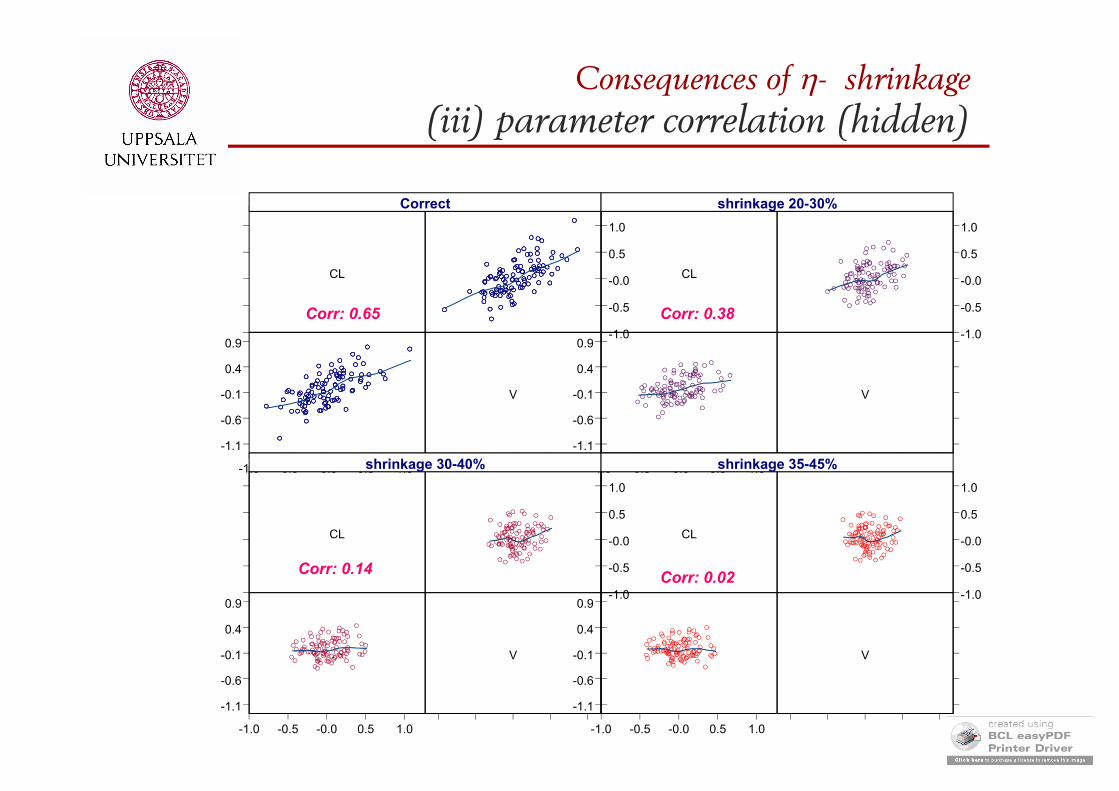
Correct shrinkage 20-30%
shrinkage 30-40% shrinkage 35-45%
Corr: 0.65 Corr: 0.38
Corr: 0.14 Corr: 0.02
Consequences of - shrinkage(iii) parameter correlation (hidden)
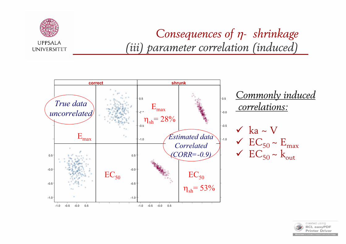
Consequences of - shrinkage(iii) parameter correlation (induced)
Commonly induced correlations:
ka ~ V EC50 ~ Emax EC50 ~ kout
ETA1
-1.0
-0.5
-0.0
0.5
-1.0 -0.5 -0.0 0.5
-1.0
-0.5
-0.0
0.5
-1.0 -0.5 -0.0 0.5
ETA2
ETA1
-1.0
-0.5
-0.0
0.5
-1.0 -0.5 -0.0 0.5
-1.0
-0.5
-0.0
0.5
-1.0 -0.5 -0.0 0.5
ETA2
correct shrunk
Emax
Emax
EC50 EC50
True datauncorrelated
Estimated dataCorrelated
(CORR=-0.9)
sh= 28%
sh= 53%
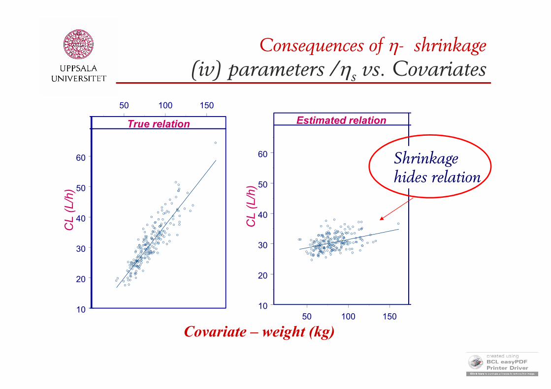
50 100 150Covariate - weight (kg)
10
20
30
40
50
60
CL
(L/h
)
Estimated relation
Consequences of - shrinkage(iv) parameters /s vs. Covariates
Shrinkagehides relation
50 100 150
True relation
Covariate – weight (kg)
10
20
30
40
50
60
CL
(L/h
)
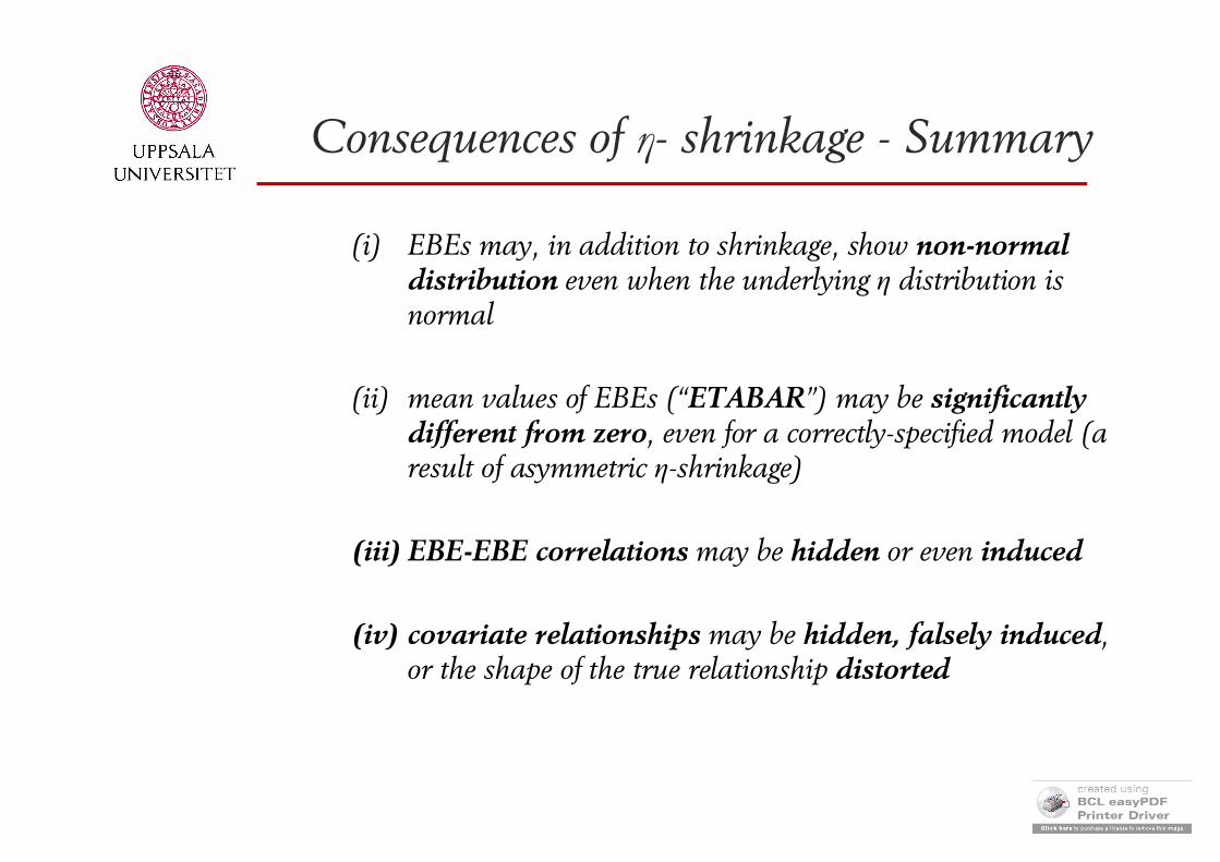
(i) EBEs may, in addition to shrinkage, show non-normal distribution even when the underlying η distribution is normal
(ii) mean values of EBEs (“ETABAR”) may be significantly different from zero, even for a correctly-specified model (a result of asymmetric η-shrinkage)
(iii) EBE-EBE correlations may be hidden or even induced
(iv) covariate relationships may be hidden, falsely induced, or the shape of the true relationship distorted
Consequences of η- shrinkage - Summary
-7
-6
-5
-7.0 -6.5 -6.0 -5.5 -5.0
2970269882233533998147438594
206356527253176449884319266
78
29
2970
98
479835
708235784326
3176720
12
84505383149729266
668449
53
673
6320
5925123973
1972
78
5392
19598
53
6684
84669249
319272
8
89272
51
31
17
10064
52
66
7349594397778090137632053
78
Basic goodness-of-fit, Run 10a
-7.0
-6.5
-6.0
-5.5
-5.0
-7.0 -6.5 -6.0 -5.5
92
68
1
483871
163118724995
837325
50557
779036
8276
68
Basic goodness-of-fit, Run 8
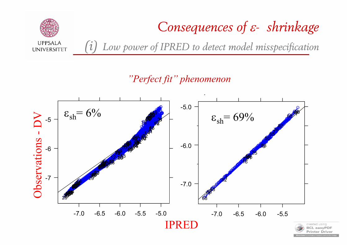
sh= 69%sh= 6%
IPRED
Obs
erva
tion
s -
DV
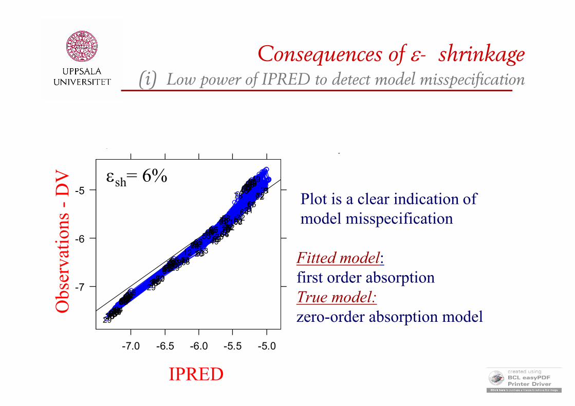
Consequences of - shrinkage(i) Low power of IPRED to detect model misspecification
Plot is a clear indication ofmodel misspecification
Fitted model:first order absorptionTrue model:zero-order absorption model
-7
-6
-5
-7.0 -6.5 -6.0 -5.5 -5.0
2970269882233533998147438594
206356527253176449884319266
78
29
2970
98
479835
708235784326
3176720
12
84505383149729266
668449
53
673
6320
5925123973
1972
78
5392
19598
53
6684
84669249
319272
8
89272
51
31
17
10064
52
66
7349594397778090137632053
78
Basic goodness-of-fit, Run 10a
-7.0
-6.5
-6.0
-5.5
-5.0
-7.0 -6.5 -6.0 -5.5
92
68
1
483871
163118724995
837325
50557
779036
8276
68
Basic goodness-of-fit, Run 8
sh= 69%sh= 6%
”Perfect fit” phenomenon
IPRED
Obs
erva
tion
s -
DV
Consequences of - shrinkage(i) Low power of IPRED to detect model misspecification

Emax model fitted to data simulated with a sigmoidal Emax model
Line of identity
Linear regression
Loess smooth
εsh = 5% εsh = 29%εsh = 13%
Obs
erva
tion
s -
DV
IPRED
Karlsson MO & Savic RM, Diagnosing model diagnostics, To appear in CPT, July 2007

11 obs/ID (3 etas)
0
2
4
6
-9 -8 -7 -6 -5
9017
98
14
80
62
60
23
1967
4
19
35
63
35
22
47
73
42
5165
9280 9
14
69
95
6795 66816953 237 49 9815
1079 63
8725 707 7252 7067 69
8252 49
6196
abs(
Ind
ivid
ual
we
ight
ed r
esi
dua
ls)
0.0
0.5
1.0
1.5
2.0
2.5
-8 -7 -6 -5
86
23
87
4
47
18
36 14
29
53
32618
29
53
252936
13
42
Individual predictions
IIW
RE
SI
Informative dataNon-shrunk IWRES
Uninformative dataShrunk IWRES
4 obs/ID (3 etas)
Misspecification indicated Misspecification NOT indicated
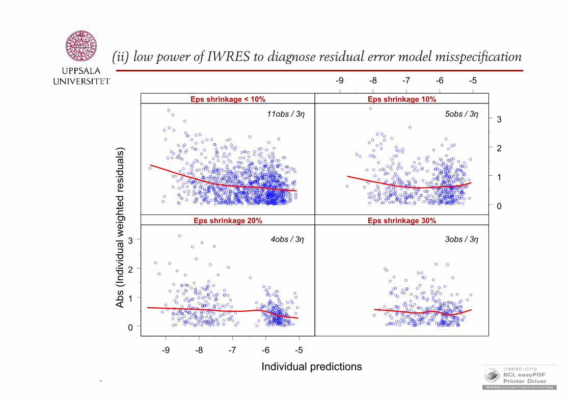
Consequences of - shrinkage(ii) Low power of IWRES to diagnose residual error
misspecification
-9 -8 -7 -6 -5
-9 -8 -7 -6 -5
Individual predictions
0
1
2
3
0
1
2
3
Ab
s (I
nd
ivid
ua
l we
igh
ted
re
sid
ua
ls)
Eps shrinkage < 10% Eps shrinkage 10%
Eps shrinkage 20% Eps shrinkage 30%
3obs / 3η
5obs / 3η
4obs / 3η
11obs / 3η
(ii) low power of IWRES to diagnose residual error model misspecification
Consequences of ε- shrinkage - Summary
(i) low power of IPRED to diagnose structural model misspecification (“perfect fit” phenomenon)
(ii) low power of IWRES to diagnose residual error model misspecification

Conclusions – part 1 Model diagnostics involving EBE, IPRED, IWRES is misleading in the presence of shrinkage
The problem of shrinkage in showed examples associated to the diagnostics solely. Estimation is not affected.
Consequences of shrinkage ignorance:- wrong decisions- increased time for data analysis- wrong models
Shrinkage phenomenon is likely to affect other type of model diagnostics such as:
- GAM- CWRES

Solutions
1. Report the shrinkage extent!- Inform modelers about relevance of the graphs
2. Estimate standard errors of ETAs - Refine EBEs and EBE-based diagnostics
3. Use other type of diagnostics- Simulation based diagnostics
4. Do more model testing inside NONMEM

EBE shrinkage & EstimationFOCE
Background:EBEs are computed at each iteration step
Question:How shrinkage may affect FOCE method?
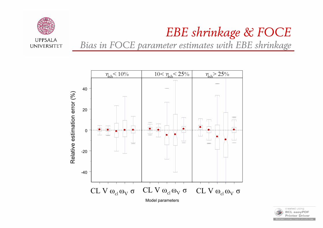
EBE shrinkage & FOCEBias in FOCE parameter estimates with EBE shrinkage
1 2 3 4 5 1 2 3 4 5 1 2 3 4 5
Model parameters
-40
-20
0
20
40
Rel
ativ
e es
timat
ion
erro
r (%
)1 2 3
CL V ωclωV σ CL V ωclωV σ CL V ωclωV σ
ηsh< 10% 10< ηsh< 25% ηsh> 25%
Conclusions - part 2
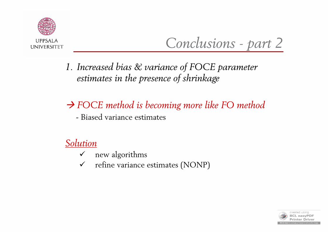
1. Increased bias & variance of FOCE parameter estimates in the presence of shrinkage
FOCE method is becoming more like FO method- Biased variance estimates
Solution new algorithms refine variance estimates (NONP)

EBE shrinkage & $NONP
1. Search for support pointsparametric step (FO/FOCE)
EBEs computation
Points of support
2. Probability estimation the joint probability the marginal cumulative probability
What if EBEs are shrunk?
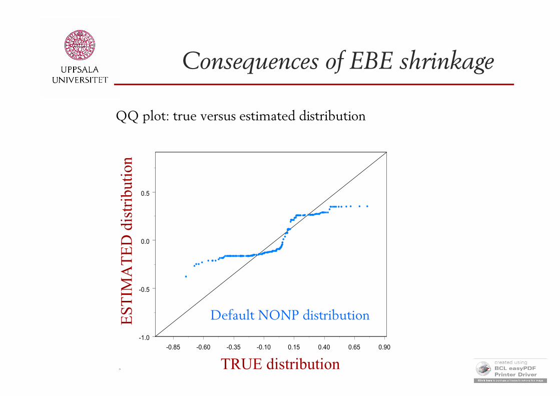
Consequences of EBE shrinkage
QQ plot: true versus estimated distribution
-0.85 -0.60 -0.35 -0.10 0.15 0.40 0.65 0.90
True distribution
-1.0
-0.5
0.0
0.5
Est
imate
d d
istr
ibutio
n
POSTHOC distributiondefault NONP distribution
TRUE distribution
ES
TIM
AT
ED
dis
trib
utio
n
Default NONP distribution

NONP and EBE shrinkageHow to proceed?
1. Keep using default NONMEM support points
range of available support points may be sufficient range of available support points lower than expected
-results still may be improved compared to the parametric outcome
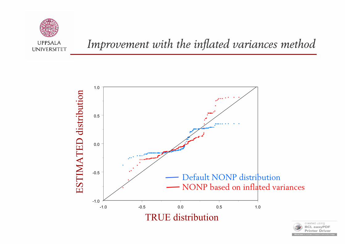
2. Inflate variances prior to EBE (POSTHOC) estimation(enough to inflate twice the variances )
-1.0 -0.5 0.0 0.5 1.0
-1.0
-0.5
0.0
0.5
1.0
Improvement with the inflated variances method
TRUE distribution
ES
TIM
AT
ED
dis
trib
utio
n
Default NONP distributionNONP based on inflated variances
NONP & EBE shrinkage - How to proceed?Enriched grid method
There is a way to enhance the NONP grid with additional points of support
Additional points of support are generated via simulations from final model
Practicaly it requrires:
simulation from the final model computation of the individual contributions to the entire
NONP density
A general routine that automizes this is under development
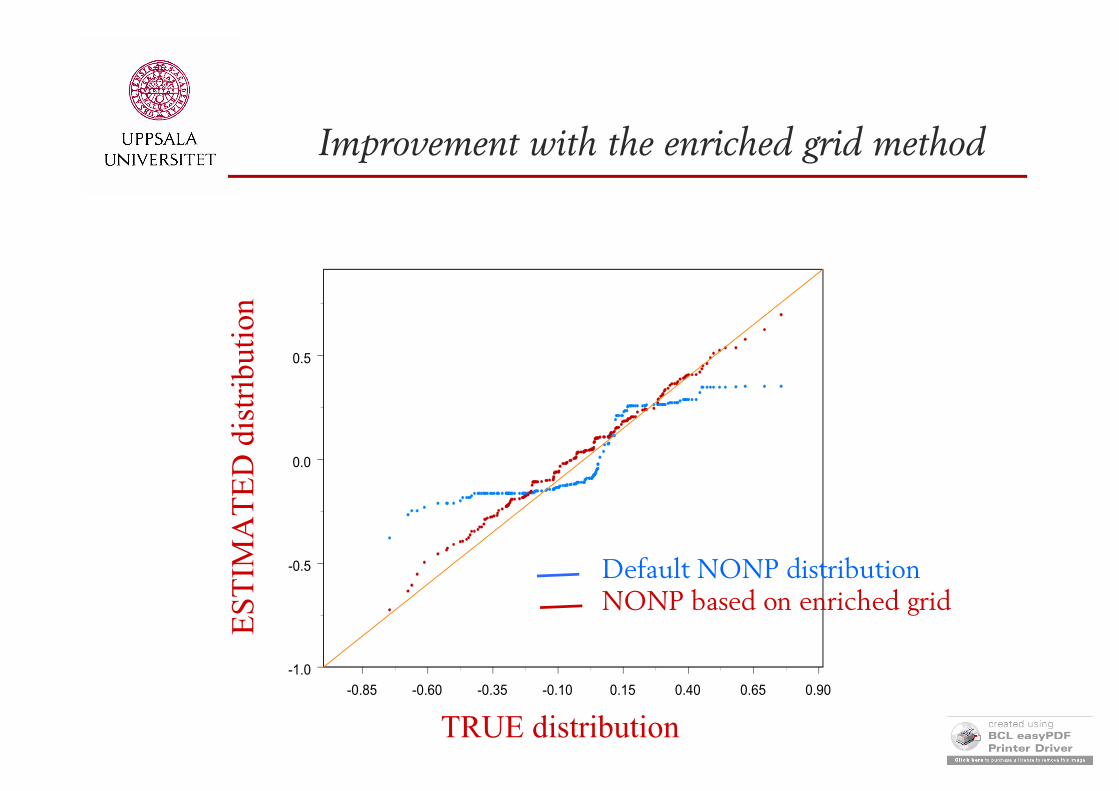
Improvement with the enriched grid method
-0.85 -0.60 -0.35 -0.10 0.15 0.40 0.65 0.90
true distribution (V)
-1.0
-0.5
0.0
0.5
POSTHOC distributionDefault NONP distributionEnriched NONP distribution
TRUE distribution
ES
TIM
AT
ED
dis
trib
utio
n
Default NONP distributionNONP based on enriched grid

Conclusions
1. Model diagnostics involving EBE, IPRED, IWRES is misleading
Essential part of model building: - wrong decisions- increased time for data analysis- wrong models
2. FOCE method is becoming more like FO methodBiased variance estimates
3. NONP method may be biasedAt higher shrinkage extents

Take-home message
Compute the shrinkage!

Solutions
1. Model diagnostics Report the shrinkage extent! Compute standard errors of ETAs Use other type of diagnostics More testing directly in NONMEM
2. FOCE new algorithms refine variance estimates (NONP)
3. NONP method Inflate varainces prior to EBE estimation Use extended grid method (soon available in PsN)
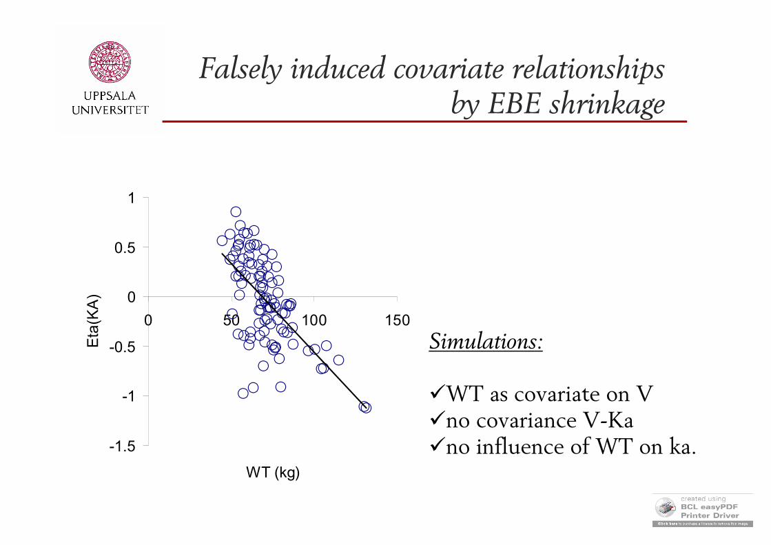
Falsely induced covariate relationships by EBE shrinkage
Simulations:
WT as covariate on V no covariance V-Kano influence of WT on ka.-1.5
-1
-0.5
0
0.5
1
0 50 100 150
WT (kg)
Eta
(KA
)