Shortest Paths & Link Weight Structure in Networks - … Paths & Link Weight Structure in Networks...

P. Van Mieghem 1Faculty of Electrical Engineering, Mathematics and Computer Science

Shortest Paths &Link Weight Structure

inNetworks

Piet Van Mieghem

CAIDA WIT (May 2006)


Introduction

The Art of Modeling

Conclusions

Outline


Telecommunication: e2e

• Main purpose: Transfer information from A B• Nearly always: Transport of packets along shortest (or optimal) paths• Optimality criterion: in terms of Quality of Service (QoS) parameters

(delay, loss, jitter, distance, monetary cost,...)• Broad focus:

What is the role of the graph/network on e2e QoS ?What is the collective behavior of flows, the network dynamics ?

A BNETWORK

G(N,L)


Fractal Nature of the Internet


Large Graphs

protein

Internet observedby RIPE boxes


Ad-hoc network

Despite node movements, at any instant in time the network can be considered as a graphwith a certain topology

Physics of the evolutionof Ad-hoc graphs


Introduction

The Art of Modeling:The Basic Model

Conclusions

Outline


Network Modeling

• Any network can be representated as a graph G with N nodes and L links:– adjaceny matrix, degree (=number of direct neighbors), connectivity,

etc... – link weight structure: importance of a link

• Link weights: also known as quality of service (QoS) parameters– delay, available capacity, loss, monetary cost, physical distance, etc...

• Assumption that transport follows shortest paths– correct in more than 70% cases in the Internet


Network ModelingConfinement to:

• Hop Count (or number of hops) of the shortest path:– Apart from end systems, QoS degradation occurs in

routers (= node).– QoS measures (packet delay, jitter, packet loss) depend on

the number of traversed routers and not on the ‘length’ of shortest path.

– Relatively easy to measure (trace-route utility) and to compute (initial assumption)

• Weight (End-to-end delay) of the shortest path:– perhaps the most interesting QoS measure for applications– difficult to measure accurately– capacity of a link:

• measurement is related to a delay measurement (dispersion of twoIP packets back-to-back)


Simple Topology Model• Link weights w(i→j )>0:

– unknown, but very likely not constant, w(i→j )≠1– assumption: i.i.d. uniformly/exponentially distributed– bi-directional links: w(i→j )= w(j→i )

• Complete graph KN• One level of complexity higher: ER Random graphs of class

Gp(N)– N: number of nodes– p: link density or probability of being edge i→j equals p– only connected graphs: p > pc ~ logN/N

5

2

43

12

2/33

1

5/2

1

Is this the right structure? Are exponential weights reasonable?Not a good model for the Internet graph, but reasonably good for Peer to Peer networks (Gnutella, KaZaa) and Ad Hoc networks


Markov Discovery Processin the complete graph KN

3) transition rates for KN: )(1, nNnnn −=+λ

1

time

t

0

node Att

tt2

t3

T

0

node A

B1

time

( ) ⎟⎟⎠

⎞⎜⎜⎝

⎛= ∑

=≤≤

n

jjjnj

aExpaExp11

)(min

1) property of i.i.d. exponential r.v.’s

2) memoryless property of exponentialdistribution


Discovery times: where τj is exponentially distributed with mean

Markov Discovery Process andUniform Recursive Tree

∑=

=k

jjkv

1τ

time

1

2

34

5

6

7

8

0

0

12 6

34

7 8

5

corresponding URTMarkovDiscoveryProcess

v1

v2

v3

v4

v5

v6

v7

v8

[ ])(

1jNj

E j −=τ

H = 0

H = 1

H = 2

H = 3

Growth rule URT:Every not yet discovered node has equal probability to beattached to any node of the URT.Hence, the number of URTswith N nodes equals (N-1)!

τ6


Uniform Recursive Tree

1

36

18

2

22

117

5

Root

12 4 9 10 15

20 17

24

14

19

21

8

13 16

23 25

1)0( =NX

5)1( =NX

9)2( =NX

7)3( =NX

4)4( =NX

26

[ ] [ ]

Nk if 0

Pr

)(

)(

≥=

==

kN

kN

N

XNXEky

[ ] [ ]∑−

=

−

=1 )1(

)(N

km

kmk

N mXEXERecursion from Growth rule URT:

Recursion for generating function: ( ) ( ) )()(1 1 zzNzN NN ϕϕ +=+ +

Solution: [ ])1()1(

)()(+Γ+Γ

+Γ==

zNzNzEz Ny

Nϕ


Hopcount of the shortest pathin KN with exp. link weights

• Shortest path (SP) described via Markov discovery process.• Shortest path tree (SPT) = Uniform recursive tree (URT) • The generating function of the hopcount HN of shortest path

between different nodes is

with

from which (via Taylor expansion around z = 0 and Stirling’sapproximation) follows that

and

[ ] ⎟⎠⎞

⎜⎝⎛ −

−=

Nz

NNzE N

H N1)(

1ϕ

)1()1()()(+Γ+Γ

+Γ=

zNzNzNϕ

[ ] ∑=

−

−≈=

k

m

mk

mN mkNNckHP

0 )!(log

[ ] 1log −+≈ γNHE N

[ ]6

logvar2πγ −+≈ NH N

close to Poisson


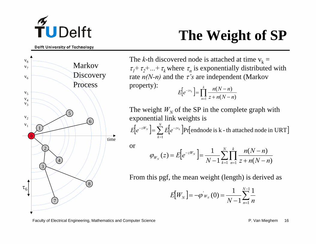
The Weight of SP

[ ] ∏=

−

−+−

=k

n

zv

nNnznNneE k

1 )()(

The k-th discovered node is attached at time vk = τ1+τ2+...+τk where τn is exponentially distributed with rate n(N-n) and the τ’s are independent (Markov property):

[ ] [ ] [ ]in URT node attachedth -k is endnodePr1

∑=

−− =N

k

zvzW kN eEeE

The weight WN of the SP in the complete graph with exponential link weights is

From this pgf, the mean weight (length) is derived as

[ ] ∑−

=−=−=

1

1

' 11

1)0(N

nWN nN

WE Nϕ

[ ] ∑∏= =

−

−+−

−==

N

k

k

n

zWW nNnz

nNnN

eEz N

N1 1 )(

)(1

1)(ϕor

time

1

2

34

5

6

7

8

0

MarkovDiscoveryProcess

v1

v2

v3

v4

v5

v6

v7

v8

τ6


Additional Results• The asymptotic distribution of the weight of the SP is

• The flooding time (= minimum time to inform all nodes in network) is

• The weight WU of the shortest path tree can be computed explicitly.

• Other instances of trees (see Multicast).• The degree distribution (= number of direct

neighbors) in the URT can be computed explicitly,

[ ] xeNN

exNNW−−

∞→=≤− logPrlim

∑ −

=− =1

11N

j jNv τ

[ ] ⎟⎟⎠

⎞⎜⎜⎝

⎛+==

−−

2

1log2PrN

NOkDk

k


Introduction

The Art of Modeling:Extension & Measurements

Conclusions

Outline


Extending the Basic Model• From the complete graph KN to the Erdös-Rényi random

graph Gp(N): from p = 1 to p < 1.• Result (which can be proved rigorously): for large N and fixed

p > pc ~ logN/N holds that the SPT in the class of Gp(N) with exponential link weights is a URT.Intuitively: Gp(N) with p > pc is sufficiently dense (there are enough links) and the link weights can be arbitrarily small such that the thinning effect of the link weights is precisely the same in all connected random graphs.

• Implications:– basic model (SPT = URT) seems more widely applicable!– influence of the link weight structure is important


Internal networksInternal networks



Internal networksInternal

networks

Border Router

TestBox D

TestBox B

TestBox C

TestBox A

MySQLDatabaseCentral

Point

The resultsISP A ISP C

ISP DISP B

Probe-packets

Border Router

Border Router

Border Router





networks

Border Router

TestBox D

TestBox B

TestBox C

TestBox A


Point


ISP DISP B

Probe-packets

Border Router

Border Router

Border Router




networks

Border Router

TestBox D

TestBox B

TestBox C

TestBox A


Point


ISP DISP B

Probe-packets

Border Router

Border Router

Border Router

RIPE measurement configuration

The traceroute data provided by RIPE NCC (the Network Coordination Centre of the Réseaux IP Européen) in the period 1998-2001.


Model and Internet measurements

0.10

0.08

0.06

0.04

0.02

0.002520151050

Measurement from RIPE fit(Log(N))=13.1

Pr[H

= k

]

E[h]=13Var[h]=21.8α =E[h]/Var[h]=0.6

hop k

[ ] ∑=

−

−≈=

k

m

mk

mN mkNNckHP

0 )!(log

2000


Model and Internet measurements

0.10

0.08

0.06

0.04

0.02

0.00

Pr[H

= k

]

302520151050

hop k

Asia Europe USA fit with log(NAsia) = 13.5 fit with log(NEurope) = 12.6 fit with log(NUSA) = 12.9

october 2004Hop k

Pr[H

= k

]


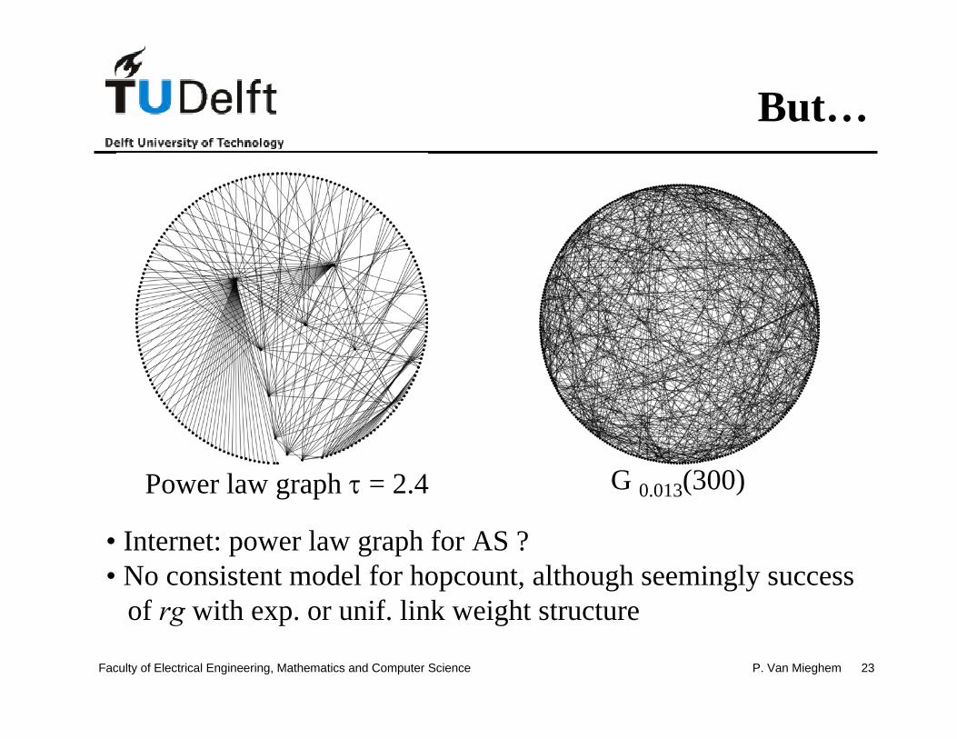
But…

Power law graph τ = 2.4 G 0.013(300)

• Internet: power law graph for AS ?• No consistent model for hopcount, although seemingly success

of rg with exp. or unif. link weight structure


Degree graphScaling law for hopcount in Degree Graph defined by Pr[D > x] = c x1-τ with mean µ = E[D]. For τ > 3, α > 0, and ak = [Logνk]-Logνk

Pr[HN – [LogνN] = k] = Pr[RaN = k] + O(logN)−α

where the random variable RaPr[Ra > k] = E[ exp{- κ νa+kW1W2}|W1W2 > 0]

with andν = E[D(D-1)]/E[D] and κ = E[D]/(ν−1)

and where W1 and W2 are independent normalized copies of a branching process. [Work in collaboration with R. van der Hofstad and G. Hooghiemstra]

Importance: (a) for each N and M where aN = aM (i.e. M=N/νk )Pr[HN>k] follows by a shift over k hops from Pr[HM>k].Hence, the hopcount for arbitrary large degree graphs (e.g. Internet?) can be simulated.(b) Currently most accurate hopcount formula

[ ] ( ) [ ]νν

νµγν log

0|log2log

1loglog21

loglog >

−−−+

−+≈WWENHE N


Introduction

The Art of Modeling:The Link Weight Structure

Conclusions

Outline


Extreme Value Index• SP is mainly determined by smallest link weights in the

distribution Fw(x) = Pr[w < x]• Taylor: Fw(x) = Fw(0) +F’w(0).x+O(x2)

= fw(0).x+O(x2)SP is not changed by scaling of link weights, hence, fw(0), can be considered as scaling factor:

1. fw(0) > 0 is finite: regular distribution2. fw(0) = 0: link weights cannot be arbitrarily small;

more influence of topology3. fw(0) →∞ : increasing prob. mass at x = 0

• Polynomial distribution: Fw(x) = xα x in [0,1]

= 1 x > 1where α is the extreme value index1. α = 1: regular distribution2. α > 1: decreasing influence w3. α < 1: increasing influence w 0 1

1

x

Fw(x)

α = 1α > 1

α < 1


Link Weight Distribution

Fw(x)

x0

α = 1 α > 1

α < 1

1ε larger scale

1For the shortestpath, onlythe smallregion aroundzero matters!


Three regimesα →∞ : – all link weights are equal to w = 1– no influence of link weights; only the topology matters

α → 1 :– link weights are regular (e.g. uniform, exponential)– SPT = URT if underlying graph is connected

α → 0 :– strong disorder: heavily fluctuating link weights in region

close to x = 0– union of all SPT is the minumum spanning tree (MST)


Average Hopcount

30

25

20

15

10

5

Ave

rage

Num

ber o

f Hop

s

3 4 5 6 7 8 9100

2 3 4 5 6 7 8 91000

Number of Nodes N

Limit: α = 0 α = 0.05 α = 0.1 α = 0.2 α = 0.4 α = 0.6 α = 0.8

p = 2 ln N/N

( )[ ]

( )[ ] ( ) 0for

1 around for ln

3/1 →=

≈

αα

αα

α

NOHE

NHE

N

N


MST and URT7

89 93 78

9827

5790

77 76

3458226

325115 36 91 42 33

56 81 73 84536761 52

406354801728 1002265 10 9 85

6727519121837

24

44

9728 344647 13

6669

58

95

68

23

60 49

99 1

117192

388320

29

86 55 41

79 59 596 31

25

70

644339 8816 21 94

50

74

48 14

35 87 4 30

62

7

64541691

434

47

79 19 97

33

85 95 39 99

80

41

45

42 8 9 31 48 57 70 56 40

81

29

43 86

100 4662

11

71

52

726328

53 89

49 50

6925

30 20 90

14 82

77

12 37

38

13

60

66

673635

44

2

84

58

3

832255

15

236

21

74

1

9826

1765 75

27

59459

51

92

10

73

98 18 2476 8868 96 78 38

(a) (b)MST (α → 0 limit) URT (α → 1 limit)

N = 100 nodes


Phase Transition1.0

0.8

0.6

0.4

0.2

0.0

Pr[G

Usp

t(α) =

MST

]

0.01 0.1 1 10

α/αc

N = 25 N = 50 N = 100 N = 200

URT-like

MST-like

∆α

αc = O(N-β)∆α = O(N-β)β around 2/3

Van Mieghem, P. and S. M. Magdalena, "A Phase Transition in the Link Weight Structure of Networks", Physical Review E, Vol. 72, November, p. 056138, (2005).


Phase Transition: implications

• Nature: superconductivity– T < Tc : macroscopic quantum effect (R = 0)– T > Tc : normal conductivity (R > 0)

• Networks:– Artifically created phase transition– if link weight structure can be changed

independently of topology, control of transport:α < αc : almost all over critical backbone (MST)α > αc : spread over more paths; load balanced

– critical backbone has minimum possible number of links N – 1: only these links need to be secured


GUspt: Union of SPTsObservable Part of a Network

• Minimum spanning tree belongs to GUspt

• Degree distribution in the overlay GUspt on the complete graph with exp. link weights is exactly known.

• Conjecture: For large N, the overlay GUspt on the ER

random graph Gp(N) with i.i.d. regular weights and

any p > pc is a connected ER graph Gpc(N).

– we have good arguments, not a rigorous proof

– important for Peer-to-peer networks!


Introduction

The Art of Modeling:

Conclusions

Outline


Summarizing• Basic SPT model: URT

– simple, analytic computations possible– reasonable first order model to approximate ad-hoc

networks, less accurate for Internet (degree!)

• Link weight structure is important: much room for research:– what is link weight structure of a real network?– what are relevant weights (delay, loss, distance, etc...?)– how to update link weights ?– if link weights can be chosen independent of topology, a

phase transition exists: steering of traffic in two modes


Summary

• Articles:http://www.nas.ewi.tudelft.nl/people/Piet

• Book: Performance Analysis of Computer Systems and Networks, Cambridge University Press (2006)

Shortest Paths & Link Weight Structure in Networks - … Paths & Link Weight Structure in Networks...

Documents

Transcript of Shortest Paths & Link Weight Structure in Networks - … Paths & Link Weight Structure in Networks...