
Short-Time Asymptotic Methods In Financial...
98
Short-Time Asymptotic Methods In Financial Mathematics José E. Figueroa-López Department of Mathematics Washington University in St. Louis ORIE, Cornell University January 18, 2017 J.E. Figueroa-López (WUSTL) Short-Time Asymptotics in Financial Mathematics ORIE, Cornell 1 / 66
Transcript of Short-Time Asymptotic Methods In Financial...
Short-Time Asymptotic Methods
In Financial Mathematics
José E. Figueroa-LópezDepartment of Mathematics
Washington University in St. Louis
ORIE, Cornell University
January 18, 2017
J.E. Figueroa-López (WUSTL) Short-Time Asymptotics in Financial Mathematics ORIE, Cornell 1 / 66
Outline
1 Overview Of Three Applications
Model Selection Using Short-Time Option Prices Asymptotics
High-Frequency Based Statistical Inference
Change-Point Detection In Continuous-Time
2 A Closer Look at Short-time Asymptotics of Option Prices Under Jumps
Out-Of-The-Money (OTM) Options
At-The-Money (ATM) Options
Applications to Parameter Calibration
3 The Problem Of Optimal Threshold Selection
J.E. Figueroa-López (WUSTL) Short-Time Asymptotics in Financial Mathematics ORIE, Cornell 2 / 66
Overview Of Three Applications
Outline
1 Overview Of Three Applications
Model Selection Using Short-Time Option Prices Asymptotics
High-Frequency Based Statistical Inference
Change-Point Detection In Continuous-Time
2 A Closer Look at Short-time Asymptotics of Option Prices Under Jumps
Out-Of-The-Money (OTM) Options
At-The-Money (ATM) Options
Applications to Parameter Calibration
3 The Problem Of Optimal Threshold Selection
J.E. Figueroa-López (WUSTL) Short-Time Asymptotics in Financial Mathematics ORIE, Cornell 3 / 66
Overview Of Three Applications Model Selection Using Short-Time Option Prices Asymptotics
Outline
1 Overview Of Three Applications
Model Selection Using Short-Time Option Prices Asymptotics
High-Frequency Based Statistical Inference
Change-Point Detection In Continuous-Time
2 A Closer Look at Short-time Asymptotics of Option Prices Under Jumps
Out-Of-The-Money (OTM) Options
At-The-Money (ATM) Options
Applications to Parameter Calibration
3 The Problem Of Optimal Threshold Selection
J.E. Figueroa-López (WUSTL) Short-Time Asymptotics in Financial Mathematics ORIE, Cornell 4 / 66
Overview Of Three Applications Model Selection Using Short-Time Option Prices Asymptotics
I. Model Selection Using Option Prices Asymptotics
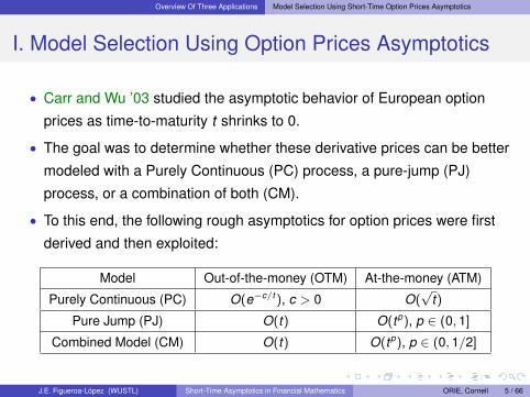
• Carr and Wu ’03 studied the asymptotic behavior of European option
prices as time-to-maturity t shrinks to 0.
• The goal was to determine whether these derivative prices can be better
modeled with a Purely Continuous (PC) process, a pure-jump (PJ)
process, or a combination of both (CM).
• To this end, the following rough asymptotics for option prices were first
derived and then exploited:
Model Out-of-the-money (OTM) At-the-money (ATM)
Purely Continuous (PC) O(e−c/t ), c > 0 O(√
t)
Pure Jump (PJ) O(t) O(tp), p ∈ (0, 1]
Combined Model (CM) O(t) O(tp), p ∈ (0, 1/2]
J.E. Figueroa-López (WUSTL) Short-Time Asymptotics in Financial Mathematics ORIE, Cornell 5 / 66
Overview Of Three Applications Model Selection Using Short-Time Option Prices Asymptotics
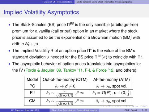
Implied Volatility Asymptotics
• The Black-Scholes (BS) price ΠBS is the only sensible (arbitrage-free)
premium for a vanilla (call or put) option in an market where the stock
price is assumed to be the exponential of a Brownian motion (BM) with
drift: σWt + µt .
• The Implied Volatility σ of an option price Π∗ is the value of the BM’s
standard deviation σ needed for the BS price ΠBS(σ) to coincide with Π∗.
• The asymptotic behavior of option prices translates into asymptotics for
the IV (Forde & Jaquier ’09, Tankov ’11, F-L & Forde ’12, and others):
Model Out-of-the-money (OTM) At-the-money (ATM)
PC σt → d 6= 0 σt → σ0, spot vol.
PJ σt ∼ |κ|√2t log(1/t)
↗∞ σt = O(tp), p ∈ (0, 12 ]
CM σt ∼ |κ|√2t log(1/t)
↗∞ σt → σ0, spot vol.
J.E. Figueroa-López (WUSTL) Short-Time Asymptotics in Financial Mathematics ORIE, Cornell 6 / 66
Overview Of Three Applications Model Selection Using Short-Time Option Prices Asymptotics
Some Implications For The IV Smile
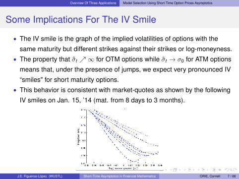
• The IV smile is the graph of the implied volatilities of options with the
same maturity but different strikes against their strikes or log-moneyness.• The property that σt ↗∞ for OTM options while σt → σ0 for ATM options
means that, under the presence of jumps, we expect very pronounced IV
“smiles" for short maturity options.• This behavior is consistent with market-quotes as shown by the following
IV smiles on Jan. 15, ’14 (mat. from 8 days to 3 months).
J.E. Figueroa-López (WUSTL) Short-Time Asymptotics in Financial Mathematics ORIE, Cornell 7 / 66
Overview Of Three Applications High-Frequency Based Statistical Inference
Outline
1 Overview Of Three Applications
Model Selection Using Short-Time Option Prices Asymptotics
High-Frequency Based Statistical Inference
Change-Point Detection In Continuous-Time
2 A Closer Look at Short-time Asymptotics of Option Prices Under Jumps
Out-Of-The-Money (OTM) Options
At-The-Money (ATM) Options
Applications to Parameter Calibration
3 The Problem Of Optimal Threshold Selection
J.E. Figueroa-López (WUSTL) Short-Time Asymptotics in Financial Mathematics ORIE, Cornell 8 / 66
Overview Of Three Applications High-Frequency Based Statistical Inference
II. HF Estimation of Integrated Variance
In econometrics, an important problem is the estimation of the integrated
variance,
IVT :=
∫ T
0σ2
s ds, (fixed T ),
for a semimartingale model
dXt = atdt + σtdWt + dJt ,
(W Standard Brownian Motion, J pure-jump process),
based on a record Xt1 , . . . ,Xtn of discrete observations of X when
mesh := maxi
(ti − ti−1)→ 0
(high-frequency or infill estimation).
J.E. Figueroa-López (WUSTL) Short-Time Asymptotics in Financial Mathematics ORIE, Cornell 9 / 66

Overview Of Three Applications High-Frequency Based Statistical Inference
Key Estimators
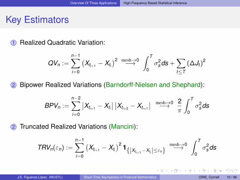
1 Realized Quadratic Variation:
QVn :=n−1∑i=0
(Xti+1 − Xti
)2 mesh→0−→∫ T
0σ2
s ds +∑t≤T
(∆Jt )2
2 Bipower Realized Variations (Barndorff-Nielsen and Shephard):
BPVn :=n−2∑i=0
∣∣Xti+1 − Xti
∣∣ ∣∣Xti+2 − Xti+1
∣∣2 Truncated Realized Variations (Mancini):
TRVn(εn) :=n−1∑i=0
(Xti+1 − Xti
)2 1{|Xti+1−Xti |≤εn}
J.E. Figueroa-López (WUSTL) Short-Time Asymptotics in Financial Mathematics ORIE, Cornell 10 / 66
Overview Of Three Applications High-Frequency Based Statistical Inference
Key Estimators
1 Realized Quadratic Variation:
QVn :=n−1∑i=0
(Xti+1 − Xti
)2 mesh→0−→∫ T
0σ2
s ds +∑t≤T
(∆Jt )2
2 Bipower Realized Variations (Barndorff-Nielsen and Shephard):
BPVn :=n−2∑i=0
∣∣Xti+1 − Xti
∣∣ ∣∣Xti+2 − Xti+1
∣∣
2 Truncated Realized Variations (Mancini):
TRVn(εn) :=n−1∑i=0
(Xti+1 − Xti
)2 1{|Xti+1−Xti |≤εn}
J.E. Figueroa-López (WUSTL) Short-Time Asymptotics in Financial Mathematics ORIE, Cornell 10 / 66
Overview Of Three Applications High-Frequency Based Statistical Inference
Key Estimators
1 Realized Quadratic Variation:
QVn :=n−1∑i=0
(Xti+1 − Xti
)2 mesh→0−→∫ T
0σ2
s ds +∑t≤T
(∆Jt )2
2 Bipower Realized Variations (Barndorff-Nielsen and Shephard):
BPVn :=n−2∑i=0
∣∣Xti+1 − Xti
∣∣ ∣∣Xti+2 − Xti+1
∣∣2 Truncated Realized Variations (Mancini):
TRVn(εn) :=n−1∑i=0
(Xti+1 − Xti
)2 1{|Xti+1−Xti |≤εn}
J.E. Figueroa-López (WUSTL) Short-Time Asymptotics in Financial Mathematics ORIE, Cornell 10 / 66
Overview Of Three Applications High-Frequency Based Statistical Inference
Key Estimators
1 Realized Quadratic Variation:
QVn :=n−1∑i=0
(Xti+1 − Xti
)2 mesh→0−→∫ T
0σ2
s ds +∑t≤T
(∆Jt )2
2 Bipower Realized Variations (Barndorff-Nielsen and Shephard):
BPVn :=n−2∑i=0
∣∣Xti+1 − Xti
∣∣ ∣∣Xti+2 − Xti+1
∣∣ mesh→0−→ 2π
∫ T
0σ2
s ds
2 Truncated Realized Variations (Mancini):
TRVn(εn) :=n−1∑i=0
(Xti+1 − Xti
)2 1{|Xti+1−Xti |≤εn}
J.E. Figueroa-López (WUSTL) Short-Time Asymptotics in Financial Mathematics ORIE, Cornell 10 / 66
Overview Of Three Applications High-Frequency Based Statistical Inference
Key Estimators
1 Realized Quadratic Variation:
QVn :=n−1∑i=0
(Xti+1 − Xti
)2 mesh→0−→∫ T
0σ2
s ds +∑t≤T
(∆Jt )2
2 Bipower Realized Variations (Barndorff-Nielsen and Shephard):
BPVn :=n−2∑i=0
∣∣Xti+1 − Xti
∣∣ ∣∣Xti+2 − Xti+1
∣∣ mesh→0−→ 2π
∫ T
0σ2
s ds
2 Truncated Realized Variations (Mancini):
TRVn(εn) :=n−1∑i=0
(Xti+1 − Xti
)2 1{|Xti+1−Xti |≤εn}mesh→0−→
∫ T
0σ2
s ds
J.E. Figueroa-López (WUSTL) Short-Time Asymptotics in Financial Mathematics ORIE, Cornell 10 / 66
Overview Of Three Applications High-Frequency Based Statistical Inference
Some Questions
• What are the infill asymptotic properties of the estimators? Asymptotic
bias, variance, CLT, etc...
• Is it better to use BPV or TRV?
• How do you calibrate or tune up the truncation parameter εn?
J.E. Figueroa-López (WUSTL) Short-Time Asymptotics in Financial Mathematics ORIE, Cornell 11 / 66
Overview Of Three Applications Change-Point Detection In Continuous-Time
Outline
1 Overview Of Three Applications
Model Selection Using Short-Time Option Prices Asymptotics
High-Frequency Based Statistical Inference
Change-Point Detection In Continuous-Time
2 A Closer Look at Short-time Asymptotics of Option Prices Under Jumps
Out-Of-The-Money (OTM) Options
At-The-Money (ATM) Options
Applications to Parameter Calibration
3 The Problem Of Optimal Threshold Selection
J.E. Figueroa-López (WUSTL) Short-Time Asymptotics in Financial Mathematics ORIE, Cornell 12 / 66
Overview Of Three Applications Change-Point Detection In Continuous-Time
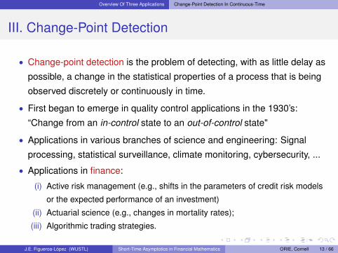
III. Change-Point Detection
• Change-point detection is the problem of detecting, with as little delay as
possible, a change in the statistical properties of a process that is being
observed discretely or continuously in time.
• First began to emerge in quality control applications in the 1930’s:
“Change from an in-control state to an out-of-control state"
• Applications in various branches of science and engineering: Signal
processing, statistical surveillance, climate monitoring, cybersecurity, ...
• Applications in finance:
(i) Active risk management (e.g., shifts in the parameters of credit risk models
or the expected performance of an investment)
(ii) Actuarial science (e.g., changes in mortality rates);
(iii) Algorithmic trading strategies.
J.E. Figueroa-López (WUSTL) Short-Time Asymptotics in Financial Mathematics ORIE, Cornell 13 / 66
Overview Of Three Applications Change-Point Detection In Continuous-Time
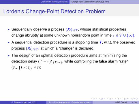
Lorden’s Change-Point Detection Problem
• Sequentially observe a process (Xt )t∈T , whose statistical properties
change abruptly at some unknown nonrandom point in time τ ∈ T ∪ {∞}.
• A sequential detection procedure is a stopping time T , w.r.t. the observed
process (Xt )t∈T , at which a “change" is declared.
• The design of an optimal detection procedure aims at minimizing the
detection delay (T − τ)1{T>τ}, while controlling the false alarm “rate"
(P∞ [T < t ] , ∀ t):
J.E. Figueroa-López (WUSTL) Short-Time Asymptotics in Financial Mathematics ORIE, Cornell 14 / 66
Overview Of Three Applications Change-Point Detection In Continuous-Time
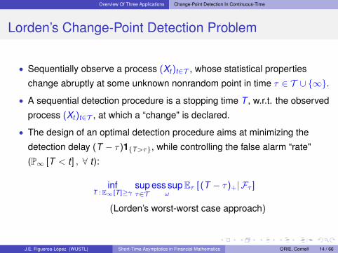
Lorden’s Change-Point Detection Problem
• Sequentially observe a process (Xt )t∈T , whose statistical properties
change abruptly at some unknown nonrandom point in time τ ∈ T ∪ {∞}.
• A sequential detection procedure is a stopping time T , w.r.t. the observed
process (Xt )t∈T , at which a “change" is declared.
• The design of an optimal detection procedure aims at minimizing the
detection delay (T − τ)1{T>τ}, while controlling the false alarm “rate"
(P∞ [T < t ] , ∀ t):
infT : E∞[T ]≥γ
supτ∈T
ess supω
Eτ [ (T − τ)+| Fτ ]
(Lorden’s worst-worst case approach)
J.E. Figueroa-López (WUSTL) Short-Time Asymptotics in Financial Mathematics ORIE, Cornell 14 / 66
Overview Of Three Applications Change-Point Detection In Continuous-Time
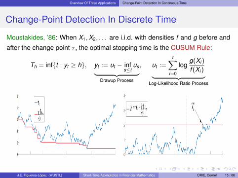
Change-Point Detection In Discrete Time
Moustakides, ’86: When X1,X2, . . . are i.i.d. with densities f and g before and
after the change point τ , the optimal stopping time is the CUSUM Rule:
Th = inf{t : yt ≥ h}, yt := ut − infs≤t
us︸ ︷︷ ︸Drawup Process
, ut :=t∑
i=0
logg(Xi )
f (Xi )︸ ︷︷ ︸Log-Likelihood Ratio Process
J.E. Figueroa-López (WUSTL) Short-Time Asymptotics in Financial Mathematics ORIE, Cornell 15 / 66
Overview Of Three Applications Change-Point Detection In Continuous-Time
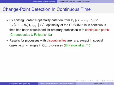
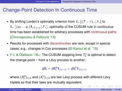
Change-Point Detection In Continuous Time
• By shifting Lorden’s optimality criterion from Eτ [ (T − τ)+| Fτ ] to
Eτ[
(uT − uτ )1{T≥τ}∣∣Fτ ], optimality of the CUSUM rule in continuous
time has been established for arbitrary processes with continuous paths
(Chronopoulou & Fellouris ’13)
• Results for processes with discontinuities are rare, except in special
cases; e.g., changes in Cox processes (El Karoui et al. ’15)
• F-L & Ólafsson ’18+: The CUSUM stopping time T ch is optimal to detect
the change point τ from a Lévy process to another:
dXt = dX 0t 1{t<τ} + dX 1
t 1{t≥τ},
where (X 0t )t≥0 and (X 1
t )t≥0 are two Lévy process with different Lévy
triplets so that their laws are mutually equivalent.
J.E. Figueroa-López (WUSTL) Short-Time Asymptotics in Financial Mathematics ORIE, Cornell 16 / 66
Overview Of Three Applications Change-Point Detection In Continuous-Time
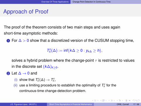
Approach of Proof
The proof of the theorem consists of two main steps and uses again
short-time asymptotic methods:
1 For ∆ > 0 show that a discretized version of the CUSUM stopping time,
T ch (∆) := inf{k∆ ≥ 0 : yk∆ ≥ h},
solves a hybrid problem where the change-point τ is restricted to values
in the discrete set (k∆)k≥0.
2 Let ∆→ 0 and
(i) show that T ch (∆)→ T c
h ,
(ii) use a limiting procedure to establish the optimality of T ch for the
continuous-time change-detection problem.
J.E. Figueroa-López (WUSTL) Short-Time Asymptotics in Financial Mathematics ORIE, Cornell 17 / 66
A Closer Look at Short-time Asymptotics of Option Prices Under Jumps
Outline
1 Overview Of Three Applications
Model Selection Using Short-Time Option Prices Asymptotics
High-Frequency Based Statistical Inference
Change-Point Detection In Continuous-Time
2 A Closer Look at Short-time Asymptotics of Option Prices Under Jumps
Out-Of-The-Money (OTM) Options
At-The-Money (ATM) Options
Applications to Parameter Calibration
3 The Problem Of Optimal Threshold Selection
J.E. Figueroa-López (WUSTL) Short-Time Asymptotics in Financial Mathematics ORIE, Cornell 18 / 66
A Closer Look at Short-time Asymptotics of Option Prices Under Jumps Out-Of-The-Money (OTM) Options
Outline
1 Overview Of Three Applications
Model Selection Using Short-Time Option Prices Asymptotics
High-Frequency Based Statistical Inference
Change-Point Detection In Continuous-Time
2 A Closer Look at Short-time Asymptotics of Option Prices Under Jumps
Out-Of-The-Money (OTM) Options
At-The-Money (ATM) Options
Applications to Parameter Calibration
3 The Problem Of Optimal Threshold Selection
J.E. Figueroa-López (WUSTL) Short-Time Asymptotics in Financial Mathematics ORIE, Cornell 19 / 66
A Closer Look at Short-time Asymptotics of Option Prices Under Jumps Out-Of-The-Money (OTM) Options
Main Result I
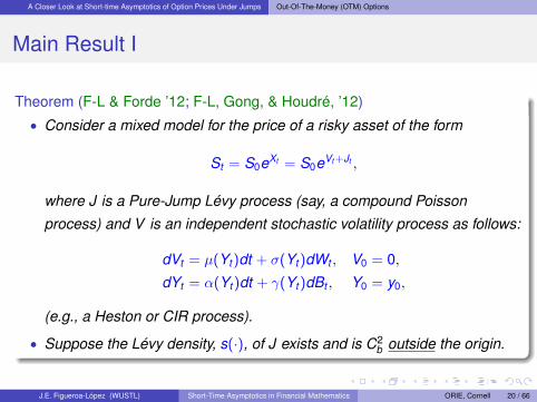
Theorem (F-L & Forde ’12; F-L, Gong, & Houdré, ’12)
• Consider a mixed model for the price of a risky asset of the form
St = S0eXt = S0eVt +Jt ,
where J is a Pure-Jump Lévy process (say, a compound Poisson
process) and V is an independent stochastic volatility process as follows:
dVt = µ(Yt )dt + σ(Yt )dWt , V0 = 0,
dYt = α(Yt )dt + γ(Yt )dBt , Y0 = y0,
(e.g., a Heston or CIR process).
• Suppose the Lévy density, s(·), of J exists and is C2b outside the origin.
J.E. Figueroa-López (WUSTL) Short-Time Asymptotics in Financial Mathematics ORIE, Cornell 20 / 66
A Closer Look at Short-time Asymptotics of Option Prices Under Jumps Out-Of-The-Money (OTM) Options
Main Result II
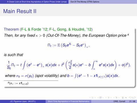
Theorem (F-L & Forde ’12; F-L, Gong, & Houdré, ’12)
Then, for any fixed κ > 0 (Out-Of-The-Money), the European Option price a
Πt := E(S0eXt − S0eκ
)+,
is such that
1S0
Πt = t∫
(ex − eκ)+ s(x)dx + t2(σ2
0
2s(κ)eκ − b
∫ ∞κ
exs(x)dx)
+ o(t2),
where σ0 = σ(y0) (spot volatility) and b =∫
(ex − 1− x1|x|≤1)s(x)dx.
a(x+ := x1x>0)
J.E. Figueroa-López (WUSTL) Short-Time Asymptotics in Financial Mathematics ORIE, Cornell 21 / 66
A Closer Look at Short-time Asymptotics of Option Prices Under Jumps Out-Of-The-Money (OTM) Options
Remarks
• As seen above, the presence of the continuous component increases the
price of the OTM option price by t2 σ20
2 s(κ)eκ(1 + o(1)).
• It can be extended to a more general class of jump processes such as
Jt =
∫ t
0
∫R\{0}
hs(x) (N(ds,dx)− s(x)dxds) ,
where N is a Poisson random measure with mean measure
µ(dx ,dt) = s(x)dxdt .
• In-The-Money (ITM) options (when κ < 0) can be handled by call-put
parity.
• In practice, the most liquid or tradable options have log-moneyness κ
“close" to 0, so it is important to consider At-The-Money (ATM) options
(namely, those with κ = 0).
J.E. Figueroa-López (WUSTL) Short-Time Asymptotics in Financial Mathematics ORIE, Cornell 22 / 66
A Closer Look at Short-time Asymptotics of Option Prices Under Jumps At-The-Money (ATM) Options
Outline
1 Overview Of Three Applications
Model Selection Using Short-Time Option Prices Asymptotics
High-Frequency Based Statistical Inference
Change-Point Detection In Continuous-Time
2 A Closer Look at Short-time Asymptotics of Option Prices Under Jumps
Out-Of-The-Money (OTM) Options
At-The-Money (ATM) Options
Applications to Parameter Calibration
3 The Problem Of Optimal Threshold Selection
J.E. Figueroa-López (WUSTL) Short-Time Asymptotics in Financial Mathematics ORIE, Cornell 23 / 66
A Closer Look at Short-time Asymptotics of Option Prices Under Jumps At-The-Money (ATM) Options
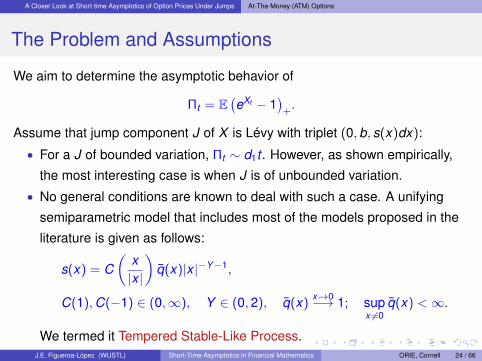
The Problem and Assumptions
We aim to determine the asymptotic behavior of
Πt = E(eXt − 1
)+.
Assume that jump component J of X is Lévy with triplet (0,b, s(x)dx):
• For a J of bounded variation, Πt ∼ d1t . However, as shown empirically,
the most interesting case is when J is of unbounded variation.
• No general conditions are known to deal with such a case. A unifying
semiparametric model that includes most of the models proposed in the
literature is given as follows:
s(x) = C(
x|x |
)q(x)|x |−Y−1,
C(1),C(−1) ∈ (0,∞), Y ∈ (0,2), q(x)x→0−→ 1; sup
x 6=0q(x) <∞.
We termed it Tempered Stable-Like Process.J.E. Figueroa-López (WUSTL) Short-Time Asymptotics in Financial Mathematics ORIE, Cornell 24 / 66
A Closer Look at Short-time Asymptotics of Option Prices Under Jumps At-The-Money (ATM) Options
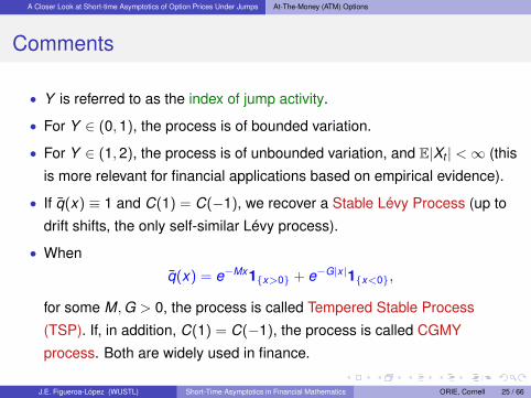
Comments
• Y is referred to as the index of jump activity.
• For Y ∈ (0,1), the process is of bounded variation.
• For Y ∈ (1,2), the process is of unbounded variation, and E|Xt | <∞ (this
is more relevant for financial applications based on empirical evidence).
• If q(x) ≡ 1 and C(1) = C(−1), we recover a Stable Lévy Process (up to
drift shifts, the only self-similar Lévy process).
• When
q(x) = e−Mx1{x>0} + e−G|x|1{x<0},
for some M,G > 0, the process is called Tempered Stable Process
(TSP). If, in addition, C(1) = C(−1), the process is called CGMY
process. Both are widely used in finance.
J.E. Figueroa-López (WUSTL) Short-Time Asymptotics in Financial Mathematics ORIE, Cornell 25 / 66
A Closer Look at Short-time Asymptotics of Option Prices Under Jumps At-The-Money (ATM) Options
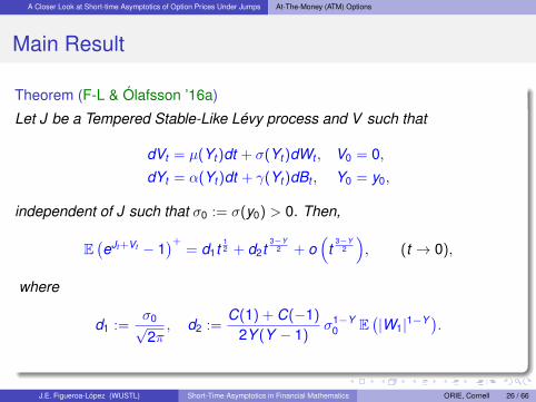
Main Result
Theorem (F-L & Ólafsson ’16a)
Let J be a Tempered Stable-Like Lévy process and V such that
dVt = µ(Yt )dt + σ(Yt )dWt , V0 = 0,
dYt = α(Yt )dt + γ(Yt )dBt , Y0 = y0,
independent of J such that σ0 := σ(y0) > 0. Then,
E(eJt +Vt − 1
)+= d1t
12 + d2t
3−Y2 + o
(t
3−Y2
), (t → 0),
where
d1 :=σ0√2π, d2 :=
C(1) + C(−1)
2Y (Y − 1)σ1−Y
0 E(|W1|1−Y ).
J.E. Figueroa-López (WUSTL) Short-Time Asymptotics in Financial Mathematics ORIE, Cornell 26 / 66
A Closer Look at Short-time Asymptotics of Option Prices Under Jumps At-The-Money (ATM) Options
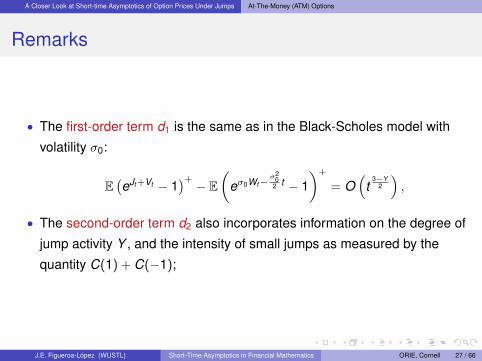
Remarks
• The first-order term d1 is the same as in the Black-Scholes model with
volatility σ0:
E(eJt +Vt − 1
)+ − E(
eσ0Wt−σ2
02 t − 1
)+
= O(
t3−Y
2
),
• The second-order term d2 also incorporates information on the degree of
jump activity Y , and the intensity of small jumps as measured by the
quantity C(1) + C(−1);
J.E. Figueroa-López (WUSTL) Short-Time Asymptotics in Financial Mathematics ORIE, Cornell 27 / 66
A Closer Look at Short-time Asymptotics of Option Prices Under Jumps At-The-Money (ATM) Options
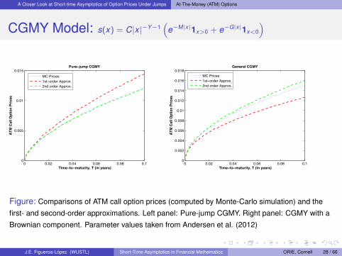
CGMY Model: s(x) = C|x |−Y−1(
e−M|x|1x>0 + e−G|x|1x<0
)
0 0.02 0.04 0.06 0.08 0.10
0.005
0.01
0.015Pure−jump CGMY
Time−to−maturity, T (in years)
ATM
Cal
l Opt
ion
Pric
es
MC Prices1st−order Approx.2nd order Approx.
0 0.02 0.04 0.06 0.08 0.10
0.002
0.004
0.006
0.008
0.01
0.012
0.014
0.016
0.018General CGMY
Time−to−maturity, T (in years)AT
M C
all O
ptio
n Pr
ices
MC Prices1st−order Approx.2nd order Approx.
Figure: Comparisons of ATM call option prices (computed by Monte-Carlo simulation) and thefirst- and second-order approximations. Left panel: Pure-jump CGMY. Right panel: CGMY with aBrownian component. Parameter values taken from Andersen et al. (2012)
J.E. Figueroa-López (WUSTL) Short-Time Asymptotics in Financial Mathematics ORIE, Cornell 28 / 66
A Closer Look at Short-time Asymptotics of Option Prices Under Jumps Applications to Parameter Calibration
Outline
1 Overview Of Three Applications
Model Selection Using Short-Time Option Prices Asymptotics
High-Frequency Based Statistical Inference
Change-Point Detection In Continuous-Time
2 A Closer Look at Short-time Asymptotics of Option Prices Under Jumps
Out-Of-The-Money (OTM) Options
At-The-Money (ATM) Options
Applications to Parameter Calibration
3 The Problem Of Optimal Threshold Selection
J.E. Figueroa-López (WUSTL) Short-Time Asymptotics in Financial Mathematics ORIE, Cornell 29 / 66
A Closer Look at Short-time Asymptotics of Option Prices Under Jumps Applications to Parameter Calibration
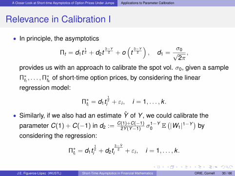
Relevance in Calibration I
• In principle, the asymptotics
Πt = d1t12 + d2t
3−Y2 + o
(t
3−Y2
), d1 =
σ0√2π,
provides us with an approach to calibrate the spot vol. σ0, given a sample
Π∗t1 , . . . ,Π∗tk of short-time option prices, by considering the linear
regression model:
Π∗ti = d1t12
i + εi , i = 1, . . . , k .
• Similarly, if we also had an estimate Y of Y , we could calibrate the
parameter C(1) + C(−1) in d2 := C(1)+C(−1)2Y (Y−1) σ1−Y
0 E(|W1|1−Y
)by
considering the regression:
Π∗ti = d1t12
i + d2t3−Y
2i + εi , i = 1, . . . , k .
J.E. Figueroa-López (WUSTL) Short-Time Asymptotics in Financial Mathematics ORIE, Cornell 30 / 66
A Closer Look at Short-time Asymptotics of Option Prices Under Jumps Applications to Parameter Calibration
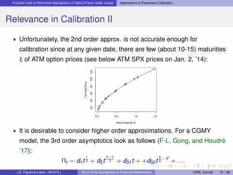
Relevance in Calibration II
• Unfortunately, the 2nd order approx. is not accurate enough for
calibration since at any given date, there are few (about 10-15) maturities
ti of ATM option prices (see below ATM SPX prices on Jan. 2, ’14):
0.0 0.5 1.0 1.5
2040
6080
100
120
time-to-maturity (t)
Cal
l Mid
Pric
e
• It is desirable to consider higher order approximations. For a CGMY
model, the 3rd order asymptotics look as follows (F-L, Gong, and Houdré
’17):
Πt = d1t12 + d2t
3−Y2 + d31t + +d32t
52−Y + . . .
J.E. Figueroa-López (WUSTL) Short-Time Asymptotics in Financial Mathematics ORIE, Cornell 31 / 66
A Closer Look at Short-time Asymptotics of Option Prices Under Jumps Applications to Parameter Calibration
Relevance in Calibration III
In that case, we can run the following regression model:
Π∗ti := d1t1/2i + d2t
3−Y2
i + d31ti + d32t52−Y
i + εi ,
where t1 < · · · < tk are the available maturities and Π∗t1 , . . . ,Π∗tk are the
observed ATM option prices. Recall that
d1 =σ0√2π, d2 =
CY (Y − 1)
σ1−Y0 E
(|W1|1−Y ) .
Remark: An estimate of Y can be obtained using HF stock data (cf.
Aït-Sahalia & Jacod, ’09) or short-time asymptotics for ATM IV skew (cf. J-F &
Ólafsson ’17).
J.E. Figueroa-López (WUSTL) Short-Time Asymptotics in Financial Mathematics ORIE, Cornell 32 / 66
A Closer Look at Short-time Asymptotics of Option Prices Under Jumps Applications to Parameter Calibration
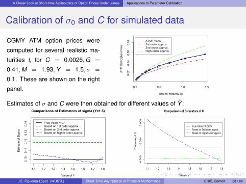
Calibration of σ0 and C for simulated data
CGMY ATM option prices were
computed for several realistic ma-
turities ti for C = 0.0026,G =
0.41,M = 1.93,Y = 1.5, σ =
0.1. These are shown on the right
panel. 0.0 0.5 1.0 1.5
0.02
0.04
0.06
0.08
time-to-maturity (t)
ATM
Cal
l Opt
ion
Pric
e
ATM Prices1st order approx.2nd order approx.High order approx.
Estimates of σ and C were then obtained for different values of Y :
1.1 1.2 1.3 1.4 1.5 1.6 1.7 1.8
0.10
0.11
0.12
0.13
0.14
Comparisons of Estimators of sigma (Y=1.5)
Value of Y
Estim
ate
of S
igm
a
True Value = 0.1Based on 1st order approx.Based on 2nd order approx.Based on higher order approx.
1.1 1.2 1.3 1.4 1.5 1.6 1.7 1.8
0.000
0.004
0.008
Comparisons of Estimators of C
Value of Y
Est
ima
te o
f C
True Value = 0.0026Based on 2nd order approx.Based on higher order approx.
J.E. Figueroa-López (WUSTL) Short-Time Asymptotics in Financial Mathematics ORIE, Cornell 33 / 66
A Closer Look at Short-time Asymptotics of Option Prices Under Jumps Applications to Parameter Calibration
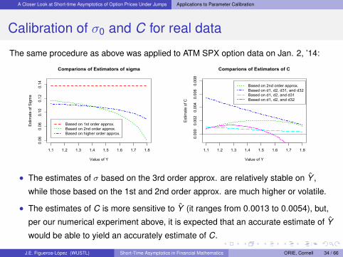
Calibration of σ0 and C for real data
The same procedure as above was applied to ATM SPX option data on Jan. 2, ’14:
1.1 1.2 1.3 1.4 1.5 1.6 1.7 1.8
0.06
0.08
0.10
0.12
0.14
Comparions of Estimators of sigma
Value of Y
Estim
ate
of S
igm
a
Based on 1st order approx.Based on 2nd order approx.Based on higher order approx.
1.1 1.2 1.3 1.4 1.5 1.6 1.7 1.8
0.0000.0020.0040.0060.008
Comparions of Estimators of C
Value of Y
Estim
ate
of C
Based on 2nd order approx.Based on d1, d2, d31, and d32Based on d1, d2, and d31Based on d1, d2, and d32
• The estimates of σ based on the 3rd order approx. are relatively stable on Y ,
while those based on the 1st and 2nd order approx. are much higher or volatile.
• The estimates of C is more sensitive to Y (it ranges from 0.0013 to 0.0054), but,
per our numerical experiment above, it is expected that an accurate estimate of Y
would be able to yield an accurately estimate of C.
J.E. Figueroa-López (WUSTL) Short-Time Asymptotics in Financial Mathematics ORIE, Cornell 34 / 66

A Closer Look at Short-time Asymptotics of Option Prices Under Jumps Applications to Parameter Calibration
Ongoing and Future Research
1 Extend the 3rd order expansions to more general models and,
furthermore, develop a general expansion formula even if the coefficients
are not explicit.
2 Small-time asymptotics of options written on Leveraged Exchange-Traded
Fund (LETF). LETF is a managed portfolio, which seeks to multiply the
instantaneous returns of a reference Exchange-Traded Fund (ETF).
3 Besides the ATM IV σ (0, t), the ATM skew and convexity of the IV,∂σ(κ,t)∂κ
∣∣∣κ=0
and ∂2σ(κ,t)∂κ2
∣∣∣κ=0
, are very important in trading and, thus, its
asymptotic behavior is of great interest. We have results for the skew but
not the convexity.
4 There is no known results for American options. It is expected that the
early exercise feature won’t affect the leading order terms of the
asymptotics but they should contribute to the high-order terms.
J.E. Figueroa-López (WUSTL) Short-Time Asymptotics in Financial Mathematics ORIE, Cornell 35 / 66
A Closer Look at Short-time Asymptotics of Option Prices Under Jumps Applications to Parameter Calibration
Ongoing and Future Research
1 Extend the 3rd order expansions to more general models and,
furthermore, develop a general expansion formula even if the coefficients
are not explicit.
2 Small-time asymptotics of options written on Leveraged Exchange-Traded
Fund (LETF). LETF is a managed portfolio, which seeks to multiply the
instantaneous returns of a reference Exchange-Traded Fund (ETF).
3 Besides the ATM IV σ (0, t), the ATM skew and convexity of the IV,∂σ(κ,t)∂κ
∣∣∣κ=0
and ∂2σ(κ,t)∂κ2
∣∣∣κ=0
, are very important in trading and, thus, its
asymptotic behavior is of great interest. We have results for the skew but
not the convexity.
4 There is no known results for American options. It is expected that the
early exercise feature won’t affect the leading order terms of the
asymptotics but they should contribute to the high-order terms.J.E. Figueroa-López (WUSTL) Short-Time Asymptotics in Financial Mathematics ORIE, Cornell 35 / 66
The Problem Of Optimal Threshold Selection
Outline
1 Overview Of Three Applications
Model Selection Using Short-Time Option Prices Asymptotics
High-Frequency Based Statistical Inference
Change-Point Detection In Continuous-Time
2 A Closer Look at Short-time Asymptotics of Option Prices Under Jumps
Out-Of-The-Money (OTM) Options
At-The-Money (ATM) Options
Applications to Parameter Calibration
3 The Problem Of Optimal Threshold Selection
J.E. Figueroa-López (WUSTL) Short-Time Asymptotics in Financial Mathematics ORIE, Cornell 36 / 66
The Problem Of Optimal Threshold Selection
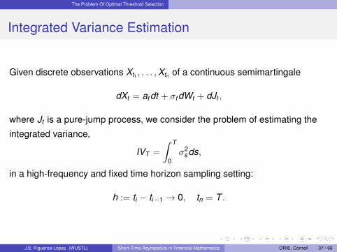
Integrated Variance Estimation
Given discrete observations Xt1 , . . . ,Xtn of a continuous semimartingale
dXt = atdt + σtdWt + dJt ,
where Jt is a pure-jump process, we consider the problem of estimating the
integrated variance,
IVT =
∫ T
0σ2
s ds,
in a high-frequency and fixed time horizon sampling setting:
h := ti − ti−1 → 0, tn = T .
J.E. Figueroa-López (WUSTL) Short-Time Asymptotics in Financial Mathematics ORIE, Cornell 37 / 66
The Problem Of Optimal Threshold Selection
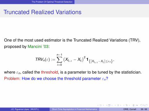
Truncated Realized Variations
One of the most used estimator is the Truncated Realized Variations (TRV),
proposed by Mancini ’03:
TRVn(ε) :=n−1∑i=0
(Xti+1 − Xti
)2 1{|Xti+1−Xti |≤εn},
where εn, called the threshold, is a parameter to be tuned by the statistician.
Problem: How do we choose the threshold parameter εn?
J.E. Figueroa-López (WUSTL) Short-Time Asymptotics in Financial Mathematics ORIE, Cornell 38 / 66

The Problem Of Optimal Threshold Selection
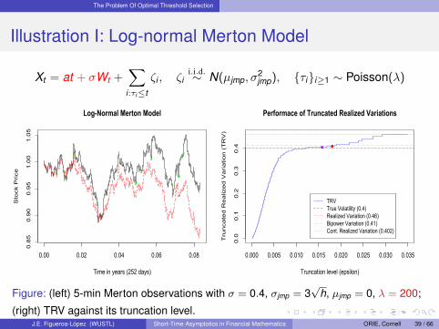
Illustration I: Log-normal Merton Model
Xt = at + σWt +∑
i:τi≤t
ζi , ζii.i.d.∼ N(µjmp, σ
2jmp), {τi}i≥1 ∼ Poisson(λ)
0.00 0.02 0.04 0.06 0.08
0.85
0.90
0.95
1.00
1.05
Log-Normal Merton Model
Time in years (252 days)
Sto
ck P
rice
0.000 0.005 0.010 0.015 0.020 0.025 0.030 0.035
0.0
0.1
0.2
0.3
0.4
Performace of Truncated Realized Variations
Truncation level (epsilon)
Tru
nca
ted
Re
aliz
ed
Va
ria
tion
(T
RV
)
TRVTrue Volatility (0.4)Realized Variation (0.46)Bipower Variation (0.41)Cont. Realized Variation (0.402)
Figure: (left) 5-min Merton observations with σ = 0.4, σjmp = 3√
h, µjmp = 0, λ = 200;
(right) TRV against its truncation level.
J.E. Figueroa-López (WUSTL) Short-Time Asymptotics in Financial Mathematics ORIE, Cornell 39 / 66
The Problem Of Optimal Threshold Selection
Illustration I: Log-normal Merton Model
Xt = at + σWt +∑
i:τi≤t
ζi , ζii.i.d.∼ N(µjmp, σ
2jmp), {τi}i≥1 ∼ Poisson(λ)
0.00 0.02 0.04 0.06 0.08
0.85
0.90
0.95
1.00
1.05
Log-Normal Merton Model
Time in years (252 days)
Sto
ck P
rice
0.000 0.005 0.010 0.015 0.020 0.025 0.030 0.035
0.0
0.1
0.2
0.3
0.4
Performace of Truncated Realized Variations
Truncation level (epsilon)
Tru
nca
ted
Re
aliz
ed
Va
ria
tion
(T
RV
)
TRVTrue Volatility (0.4)Realized Variation (0.46)Bipower Variation (0.41)Cont. Realized Variation (0.402)
Figure: (left) 5-min Merton observations with σ = 0.4, σjmp = 3√
h, µjmp = 0, λ = 200;
(right) TRV against its truncation level.J.E. Figueroa-López (WUSTL) Short-Time Asymptotics in Financial Mathematics ORIE, Cornell 39 / 66
The Problem Of Optimal Threshold Selection
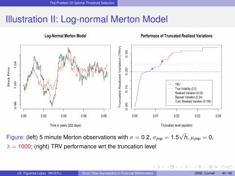
Illustration II: Log-normal Merton Model
0.00 0.02 0.04 0.06 0.08
0.96
1.00
1.04
Log-Normal Merton Model
Time in years (252 days)
Sto
ck P
rice
0.00 0.01 0.02 0.03 0.04
0.00
0.10
0.20
0.30
Performace of Truncated Realized Variations
Truncation level (epsilon)T
run
ca
ted
Re
aliz
ed
Va
ria
tio
n (
TR
V)
TRVTrue Volatility (0.2)Realized Variation (0.33)Bipower Variation (0.24)Cont. Realized Variation (0.195)
Figure: (left) 5 minute Merton observations with σ = 0.2, σjmp = 1.5√
h, µjmp = 0,
λ = 1000; (right) TRV performance wrt the truncation level
J.E. Figueroa-López (WUSTL) Short-Time Asymptotics in Financial Mathematics ORIE, Cornell 40 / 66
The Problem Of Optimal Threshold Selection
Approach To Select The Threshold
1 Fix a sensible metric of the estimation error (typically, the Mean-Square
Error);
2 Show the existence of a unique optimal threshold ε?n that minimizes the
chosen metric;
3 Analyze the (infill) asymptotic behavior ε?n (when n→∞) to
• determine its dependence on the underlying parameters of the model• Devise a plug-in type calibration of ε∗n by estimating those parameters (if
possible).
J.E. Figueroa-López (WUSTL) Short-Time Asymptotics in Financial Mathematics ORIE, Cornell 41 / 66
The Problem Of Optimal Threshold Selection
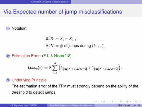
Via Expected number of jump misclassifications
1 Notation:
∆ni X := Xti − Xti−1
∆ni N := # of jumps during (ti−1, ti ]
2 Estimation Error: (F-L & Nisen ’13)
Lossn(ε) := En∑
i=1
(1[|∆n
i X |>ε,∆ni N=0] + 1[|∆n
i X |≤ε,∆ni N 6=0]
).
3 Underlying Principle
The estimation error of the TRV must strongly depend on the ability of the
threshold to detect jumps.
J.E. Figueroa-López (WUSTL) Short-Time Asymptotics in Financial Mathematics ORIE, Cornell 42 / 66
The Problem Of Optimal Threshold Selection
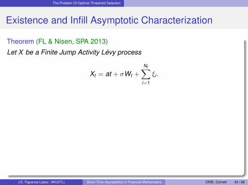
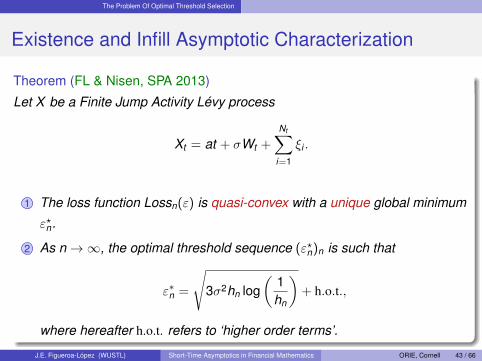
Existence and Infill Asymptotic Characterization
Theorem (FL & Nisen, SPA 2013)
Let X be a Finite Jump Activity Lévy process
Xt = at + σWt +
Nt∑i=1
ξi .
1 The loss function Lossn(ε) is quasi-convex with a unique global minimum
ε?n.
2 As n→∞, the optimal threshold sequence (ε?n)n is such that
ε∗n =
√3σ2hn log
(1hn
)+ h.o.t.,
where hereafter h.o.t. refers to ‘higher order terms’.
J.E. Figueroa-López (WUSTL) Short-Time Asymptotics in Financial Mathematics ORIE, Cornell 43 / 66

The Problem Of Optimal Threshold Selection
Existence and Infill Asymptotic Characterization
Theorem (FL & Nisen, SPA 2013)
Let X be a Finite Jump Activity Lévy process
Xt = at + σWt +
Nt∑i=1
ξi .
1 The loss function Lossn(ε) is quasi-convex with a unique global minimum
ε?n.
2 As n→∞, the optimal threshold sequence (ε?n)n is such that
ε∗n =
√3σ2hn log
(1hn
)+ h.o.t.,
where hereafter h.o.t. refers to ‘higher order terms’.
J.E. Figueroa-López (WUSTL) Short-Time Asymptotics in Financial Mathematics ORIE, Cornell 43 / 66

The Problem Of Optimal Threshold Selection
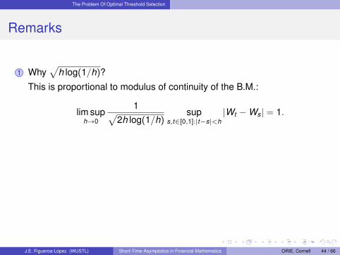
Remarks
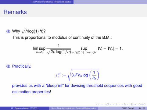
1 Why√
h log(1/h)?
This is proportional to modulus of continuity of the B.M.:
lim suph→0
1√2h log(1/h)
sups,t∈[0,1]:|t−s|<h
|Wt −Ws| = 1.
2 Practically,
ε?1n :=
√3σ2hn log
(1hn
)provides us with a “blueprint" for devising threshold sequences with good
estimation properties!
J.E. Figueroa-López (WUSTL) Short-Time Asymptotics in Financial Mathematics ORIE, Cornell 44 / 66

The Problem Of Optimal Threshold Selection
Remarks
1 Why√
h log(1/h)?
This is proportional to modulus of continuity of the B.M.:
lim suph→0
1√2h log(1/h)
sups,t∈[0,1]:|t−s|<h
|Wt −Ws| = 1.
2 Practically,
ε?1n :=
√3σ2hn log
(1hn
)provides us with a “blueprint" for devising threshold sequences with good
estimation properties!
J.E. Figueroa-López (WUSTL) Short-Time Asymptotics in Financial Mathematics ORIE, Cornell 44 / 66
The Problem Of Optimal Threshold Selection
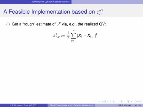
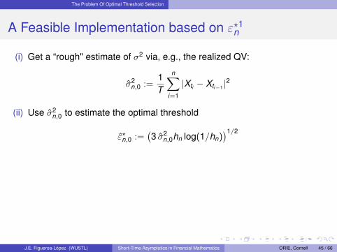
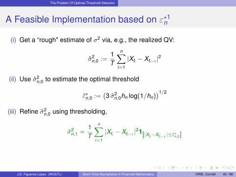
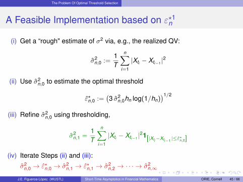
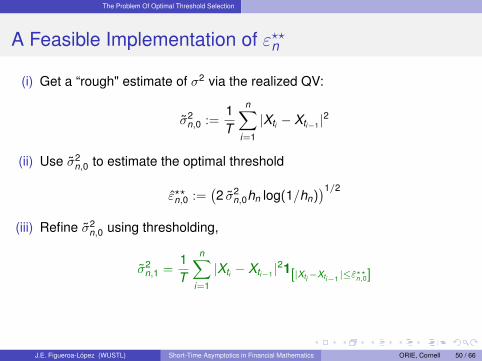
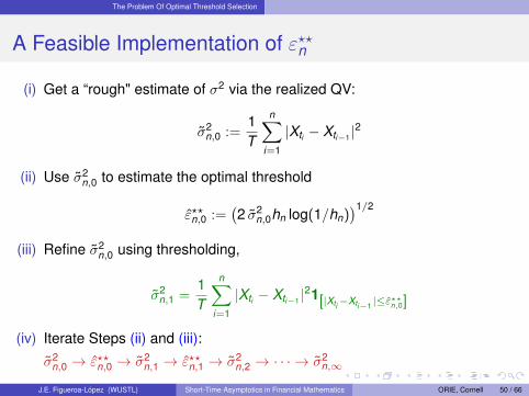
A Feasible Implementation based on ε?1n
(i) Get a “rough" estimate of σ2 via, e.g., the realized QV:
σ2n,0 :=
1T
n∑i=1
|Xti − Xti−1 |2
(ii) Use σ2n,0 to estimate the optimal threshold
ε?n,0 :=(3 σ2
n,0hn log(1/hn))1/2
(iii) Refine σ2n,0 using thresholding,
σ2n,1 =
1T
n∑i=1
|Xti − Xti−1 |21[|Xti−Xti−1 |≤ε?n,0]
(iv) Iterate Steps (ii) and (iii):
σ2n,0 → ε?n,0 → σ2
n,1 → ε?n,1 → σ2n,2 → · · · → σ2
n,∞
J.E. Figueroa-López (WUSTL) Short-Time Asymptotics in Financial Mathematics ORIE, Cornell 45 / 66
The Problem Of Optimal Threshold Selection
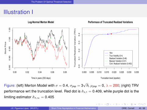
Illustration I
0.00 0.02 0.04 0.06 0.08
0.85
0.90
0.95
1.00
1.05
Log-Normal Merton Model
Time in years (252 days)
Sto
ck P
rice
0.000 0.005 0.010 0.015 0.020 0.025 0.030 0.035
0.0
0.1
0.2
0.3
0.4
Performace of Truncated Realized Variations
Truncation level (epsilon)T
run
ca
ted
Re
aliz
ed
Va
ria
tio
n (
TR
V)
TRVTrue Volatility (0.4)Realized Variation (0.46)Bipower Variation (0.41)Cont. Realized Variation (0.402)
Figure: (left) Merton Model with σ = 0.4, σjmp = 3√
h, µjmp = 0, λ = 200; (right) TRV
performance wrt the truncation level. Red dot is σn,1 = 0.409, while purple dot is the
limiting estimator σn,∞ = 0.405
J.E. Figueroa-López (WUSTL) Short-Time Asymptotics in Financial Mathematics ORIE, Cornell 46 / 66
The Problem Of Optimal Threshold Selection
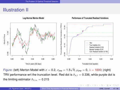
Illustration II
0.00 0.02 0.04 0.06 0.08
0.96
1.00
1.04
Log-Normal Merton Model
Time in years (252 days)
Sto
ck P
rice
0.00 0.01 0.02 0.03 0.04
0.00
0.10
0.20
0.30
Performace of Truncated Realized Variations
Truncation level (epsilon)T
run
ca
ted
Re
aliz
ed
Va
ria
tio
n (
TR
V)
TRVTrue Volatility (0.2)Realized Variation (0.33)Bipower Variation (0.24)Cont. Realized Variation (0.195)
Figure: (left) Merton Model with σ = 0.2, σjmp = 1.5√
h, µjmp = 0, λ = 1000; (right)
TRV performance wrt the truncation level. Red dot is σn,1 = 0.336, while purple dot is
the limiting estimator σn,∞ = 0.215
J.E. Figueroa-López (WUSTL) Short-Time Asymptotics in Financial Mathematics ORIE, Cornell 47 / 66
The Problem Of Optimal Threshold Selection
Via conditional Mean Square Error (cMSE)
1 We now propose a second approach in which we aim to control the
conditional MSE:
MSEc(ε) := E
(TRVn(ε)−∫ T
0σ2
s ds
)2∣∣∣∣∣∣σ·, J·
.2 Assumptions:
σt > 0, ∀ t , and σ and J are independent of W .
J.E. Figueroa-López (WUSTL) Short-Time Asymptotics in Financial Mathematics ORIE, Cornell 48 / 66
The Problem Of Optimal Threshold Selection
Via conditional Mean Square Error (cMSE)
1 We now propose a second approach in which we aim to control the
conditional MSE:
MSEc(ε) := E
(TRVn(ε)−∫ T
0σ2
s ds
)2∣∣∣∣∣∣σ·, J·
.
2 Assumptions:
σt > 0, ∀ t , and σ and J are independent of W .
J.E. Figueroa-López (WUSTL) Short-Time Asymptotics in Financial Mathematics ORIE, Cornell 48 / 66
The Problem Of Optimal Threshold Selection
Via conditional Mean Square Error (cMSE)
1 We now propose a second approach in which we aim to control the
conditional MSE:
MSEc(ε) := E
(TRVn(ε)−∫ T
0σ2
s ds
)2∣∣∣∣∣∣σ·, J·
.2 Assumptions:
σt > 0, ∀ t , and σ and J are independent of W .
J.E. Figueroa-López (WUSTL) Short-Time Asymptotics in Financial Mathematics ORIE, Cornell 48 / 66
The Problem Of Optimal Threshold Selection
Infill Asymptotics under Finite Jump Activity
Theorem (F-L & Mancini (2017))
Suppose that σt ≡ σ is constant and J is an arbitrary finite jump activity
process. Then, as n→∞, the optimal threshold ε??n is such that
ε??n ∼
√2σ2hn log
(1hn
)For time-varying volatilities t → σt , we have:
ε??n ∼√
2σ2hn ln(1/hn), n→∞,
where
σ := maxs∈[0,T ]
σs.
J.E. Figueroa-López (WUSTL) Short-Time Asymptotics in Financial Mathematics ORIE, Cornell 49 / 66

The Problem Of Optimal Threshold Selection
A Feasible Implementation of ε??n
(i) Get a “rough" estimate of σ2 via the realized QV:
σ2n,0 :=
1T
n∑i=1
|Xti − Xti−1 |2
(ii) Use σ2n,0 to estimate the optimal threshold
ε??n,0 :=(2 σ2
n,0hn log(1/hn))1/2
(iii) Refine σ2n,0 using thresholding,
σ2n,1 =
1T
n∑i=1
|Xti − Xti−1 |21[|Xti−Xti−1 |≤ε??n,0]
(iv) Iterate Steps (ii) and (iii):
σ2n,0 → ε??n,0 → σ2
n,1 → ε??n,1 → σ2n,2 → · · · → σ2
n,∞
J.E. Figueroa-López (WUSTL) Short-Time Asymptotics in Financial Mathematics ORIE, Cornell 50 / 66
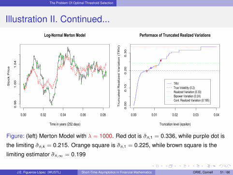
The Problem Of Optimal Threshold Selection
Illustration II. Continued...
0.00 0.02 0.04 0.06 0.08
0.96
1.00
1.04
Log-Normal Merton Model
Time in years (252 days)
Sto
ck P
rice
0.00 0.01 0.02 0.03 0.04
0.00
0.10
0.20
0.30
Performace of Truncated Realized Variations
Truncation level (epsilon)T
run
ca
ted
Re
aliz
ed
Va
ria
tio
n (
TR
V)
TRVTrue Volatility (0.2)Realized Variation (0.33)Bipower Variation (0.24)Cont. Realized Variation (0.195)
Figure: (left) Merton Model with λ = 1000. Red dot is σn,1 = 0.336, while purple dot is
the limiting σn,k = 0.215. Orange square is σn,1 = 0.225, while brown square is the
limiting estimator σn,∞ = 0.199
J.E. Figueroa-López (WUSTL) Short-Time Asymptotics in Financial Mathematics ORIE, Cornell 51 / 66
The Problem Of Optimal Threshold Selection
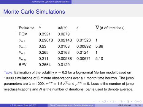
Monte Carlo Simulations
Estimator σ std(σ) ε N (# of iterations)
RQV 0.3921 0.0279
σn,1 0.29618 0.02148 0.01523 1
σn,∞ 0.23 0.0108 0.00892 5.86
σn,1 0.265 0.0163 0.0124 1
σn,∞ 0.211 0.00588 0.00671 5.10
BPV 0.2664 0.0129
Table: Estimation of the volatility σ = 0.2 for a log-normal Merton model based on
10000 simulations of 5-minute observations over a 1 month time horizon. The jump
parameters are λ = 1000, σJmp = 1.5√
h and µJmp = 0. Loss is the number of jump
misclassifications and N is the number of iterations. bar is used to denote average.
J.E. Figueroa-López (WUSTL) Short-Time Asymptotics in Financial Mathematics ORIE, Cornell 52 / 66
The Problem Of Optimal Threshold Selection
Main Breakthroughs
1 Introduced for the first time an objective threshold selection procedure
based on arguments of statistical optimality.
2 Developed the infill asymptotic characterization of the optimal thresholds.
3 Proposed an iterative algorithm to find the optimal threshold sequence.
4 Proposed extensions to more general stochastic models, which allows
time-varying stochastic volatility and jump intensity.
J.E. Figueroa-López (WUSTL) Short-Time Asymptotics in Financial Mathematics ORIE, Cornell 53 / 66
The Problem Of Optimal Threshold Selection
Ongoing and Future Research
1 In principle, we can apply the constant-volatility method for varying
volatility t → σt by localization; i.e., applying it to periods where σ is
approximately constant.
2 This could also help us to estimate σ = maxs∈[0,T ] σs and, then, apply the
asymptotic equivalence
ε??n ∼√
2σ2hn ln(1/hn).
J.E. Figueroa-López (WUSTL) Short-Time Asymptotics in Financial Mathematics ORIE, Cornell 54 / 66
The Problem Of Optimal Threshold Selection
Ongoing and Future Research
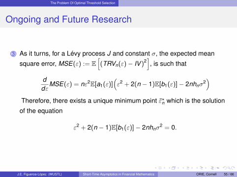
3 As it turns, for a Lévy process J and constant σ, the expected mean
square error, MSE(ε) := E[(TRVn(ε)− IV )2
], is such that
ddε
MSE(ε) = nε2E[a1(ε)](ε2 + 2(n − 1)E[b1(ε)]− 2nhnσ
2)
Therefore, there exists a unique minimum point ε?n which is the solution
of the equation
ε2 + 2(n − 1)E[b1(ε)]− 2nhnσ2 = 0.
J.E. Figueroa-López (WUSTL) Short-Time Asymptotics in Financial Mathematics ORIE, Cornell 55 / 66
The Problem Of Optimal Threshold Selection
Ongoing and Future Research
3 As it turns, for a Lévy process J and constant σ, the expected mean
square error, MSE(ε) := E[(TRVn(ε)− IV )2
], is such that
ddε
MSE(ε) = nε2E[a1(ε)](ε2 + 2(n − 1)E[b1(ε)]− 2nhnσ
2)
Therefore, there exists a unique minimum point ε?n which is the solution
of the equation
ε2 + 2(n − 1)E[b1(ε)]− 2nhnσ2 = 0.
J.E. Figueroa-López (WUSTL) Short-Time Asymptotics in Financial Mathematics ORIE, Cornell 55 / 66

The Problem Of Optimal Threshold Selection
Ongoing and Future Research
3 It can be shown that
• for a finite jump activity process,
ε?n ∼
√2σ2hn log
(1hn
)• But, surprisingly, if J is a Y -stable Lévy process (IA),
ε?n ∼
√(2− Y )σ2hn log
(1hn
)Thus the higher the jump activity is, the lower the optimal threshold has to be
to discard the higher noise represented by the jumps.
Problems: Does the above asymptotics holds for the minimizer ε?n of the cMSE?
Can we generalize it to Lévy processes with stable like jumps?
J.E. Figueroa-López (WUSTL) Short-Time Asymptotics in Financial Mathematics ORIE, Cornell 56 / 66

The Problem Of Optimal Threshold Selection
Ongoing and Future Research
3 It can be shown that
• for a finite jump activity process,
ε?n ∼
√2σ2hn log
(1hn
)
• But, surprisingly, if J is a Y -stable Lévy process (IA),
ε?n ∼
√(2− Y )σ2hn log
(1hn
)Thus the higher the jump activity is, the lower the optimal threshold has to be
to discard the higher noise represented by the jumps.
Problems: Does the above asymptotics holds for the minimizer ε?n of the cMSE?
Can we generalize it to Lévy processes with stable like jumps?
J.E. Figueroa-López (WUSTL) Short-Time Asymptotics in Financial Mathematics ORIE, Cornell 56 / 66

The Problem Of Optimal Threshold Selection
Ongoing and Future Research
3 It can be shown that
• for a finite jump activity process,
ε?n ∼
√2σ2hn log
(1hn
)• But, surprisingly, if J is a Y -stable Lévy process (IA),
ε?n ∼
√(2− Y )σ2hn log
(1hn
)Thus the higher the jump activity is, the lower the optimal threshold has to be
to discard the higher noise represented by the jumps.
Problems: Does the above asymptotics holds for the minimizer ε?n of the cMSE?
Can we generalize it to Lévy processes with stable like jumps?
J.E. Figueroa-López (WUSTL) Short-Time Asymptotics in Financial Mathematics ORIE, Cornell 56 / 66

The Problem Of Optimal Threshold Selection
Ongoing and Future Research
3 It can be shown that
• for a finite jump activity process,
ε?n ∼
√2σ2hn log
(1hn
)• But, surprisingly, if J is a Y -stable Lévy process (IA),
ε?n ∼
√(2− Y )σ2hn log
(1hn
)Thus the higher the jump activity is, the lower the optimal threshold has to be
to discard the higher noise represented by the jumps.
Problems: Does the above asymptotics holds for the minimizer ε?n of the cMSE?
Can we generalize it to Lévy processes with stable like jumps?
J.E. Figueroa-López (WUSTL) Short-Time Asymptotics in Financial Mathematics ORIE, Cornell 56 / 66
Further Reading I
J.E. Figueroa-López and S. Ólafsson,
Change-point detection for Levy processes.
To Appear in Annals of Applied Probability, 2018+.
J.E. Figueroa-López, and M. Forde,
The small-maturity smile for exponential Lévy models .
SIAM Journal on Financial Mathematics 3(1), 33-65, 2012.
J.E. Figueroa-López, R. Gong, and C. Houdré,
High-order short-time expansions for ATM option prices of exponential
Lévy models.
Mathematical Finance, 26(3), 516-557, 2016.
J.E. Figueroa-López (WUSTL) Short-Time Asymptotics in Financial Mathematics ORIE, Cornell 57 / 66
Further Reading II
J.E. Figueroa-López and S. Ólafsson,
Short-time expansions for close-to-the-money options under a Lévy jump
model with stochastic volatility.
Finance & Stochastics 20(1), 219-265, 2016a.
J.E. Figueroa-López and S. Ólafsson,
Short-time asymptotics for the implied volatility skew under a stochastic
volatility model with Lévy jumps.
Finance & Stochastics 20(4), 973-1020, 2016b.
J.E. Figueroa-López, R. Gong, and C. Houdré,
Third-Order Short-Time Expansions for Close-to-the-Money Option
Prices Under the CGMY Model.
To Appear in Journal of Applied Mathematical Finance, 2018+.
J.E. Figueroa-López (WUSTL) Short-Time Asymptotics in Financial Mathematics ORIE, Cornell 58 / 66

Further Reading III
J.E. Figueroa-López & J. Nisen.
Optimally Thresholded Realized Power Variations for Lévy Jump Diffusion
Models.
Stochastic Processes and their Applications 123(7), 2648-2677, 2013.
J.E. Figueroa-López & C. Mancini.
Optimum thresholding using mean and conditional mean square error.
Under revision in The Journal of Econometrics. Available at
https://pages.wustl.edu/figueroa, 2017.
J.E. Figueroa-López, C. Li, & J. Nisen.
Optimal iterative threshold-kernel estimation of jump diffusion processes.
In preparation, 2018.
J.E. Figueroa-López (WUSTL) Short-Time Asymptotics in Financial Mathematics ORIE, Cornell 59 / 66
Classical Path
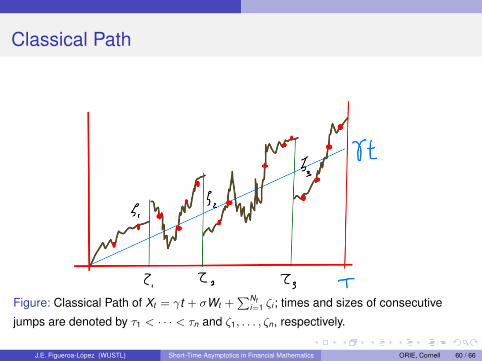
Figure: Classical Path of Xt = γt + σWt +∑Nt
i=1 ζi ; times and sizes of consecutive
jumps are denoted by τ1 < · · · < τn and ζ1, . . . , ζn, respectively.
J.E. Figueroa-López (WUSTL) Short-Time Asymptotics in Financial Mathematics ORIE, Cornell 60 / 66
The ATM Skew
• The skew of the smile is defined as the slope of the IV smile. The ATM
skew is the slope of the smile when the log-moneyness κ is 0:
∂σ (κ, t)∂κ
∣∣∣∣κ=0
,
where σ (κ, t) is the IV of an European option with log-moneyness κ and
time-to-maturity t .
• The ATM skew is actively monitored in practice by traders and analysts,
stemming in part from its rich informational content.
• Furthermore, considerable empirical support has been provided for its
significance in predicting future equity returns, and as an indicator of the
risk of large negative jumps.
J.E. Figueroa-López (WUSTL) Short-Time Asymptotics in Financial Mathematics ORIE, Cornell 61 / 66
Asymptotic Behavior of The Skew
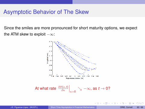
Since the smiles are more pronounced for short maturity options, we expect
the ATM skew to exploit −∞:
At what rate ∂σ(κ,t)∂κ
∣∣∣κ=0↘ −∞, as t → 0?
J.E. Figueroa-López (WUSTL) Short-Time Asymptotics in Financial Mathematics ORIE, Cornell 62 / 66
Short-time ATM Skew Asymptotics
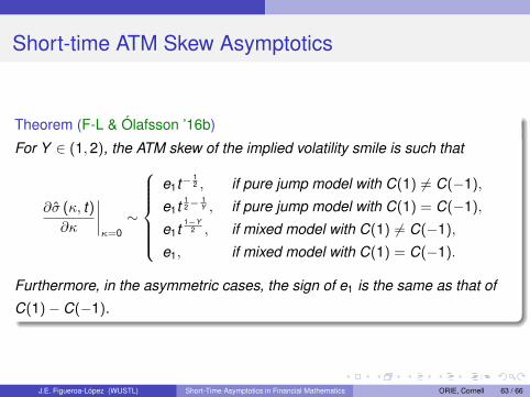
Theorem (F-L & Ólafsson ’16b)
For Y ∈ (1,2), the ATM skew of the implied volatility smile is such that
∂σ (κ, t)∂κ
∣∣∣∣κ=0∼
e1t−
12 , if pure jump model with C(1) 6= C(−1),
e1t12−
1Y , if pure jump model with C(1) = C(−1),
e1t1−Y
2 , if mixed model with C(1) 6= C(−1),
e1, if mixed model with C(1) = C(−1).
Furthermore, in the asymmetric cases, the sign of e1 is the same as that of
C(1)− C(−1).
J.E. Figueroa-López (WUSTL) Short-Time Asymptotics in Financial Mathematics ORIE, Cornell 63 / 66
ATM Skew and Implied Volatility Smile
Time-to-maturity (t)0 0.1 0.2 0.3 0.4 0.5 0.6 0.7 0.8 0.9 1
ATM
skew
-12
-10
-8
-6
-4
-2
(a)
log-moneyness (κ)-0.05 -0.04 -0.03 -0.02 -0.01 0 0.01 0.02 0.03 0.04 0.05
Implied
vol.
0.07
0.08
0.09
0.1
0.11
0.12
0.13
0.14(b)
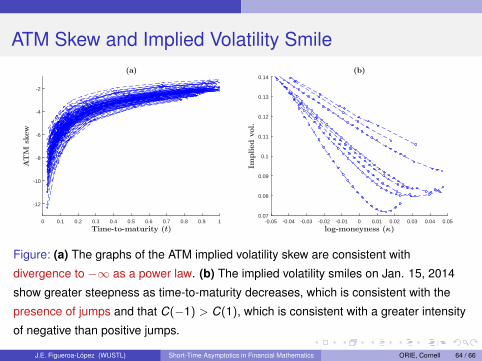
Figure: (a) The graphs of the ATM implied volatility skew are consistent with
divergence to −∞ as a power law. (b) The implied volatility smiles on Jan. 15, 2014
show greater steepness as time-to-maturity decreases, which is consistent with the
presence of jumps and that C(−1) > C(1), which is consistent with a greater intensity
of negative than positive jumps.
J.E. Figueroa-López (WUSTL) Short-Time Asymptotics in Financial Mathematics ORIE, Cornell 64 / 66
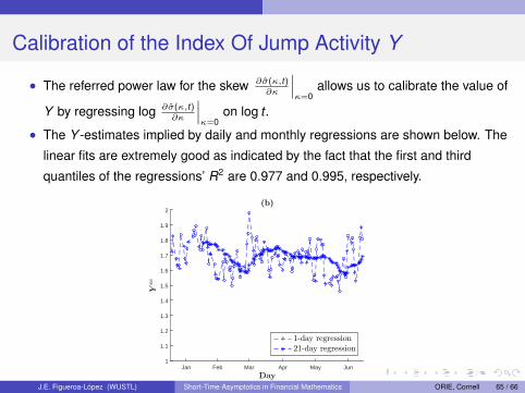
Calibration of the Index Of Jump Activity Y
• The referred power law for the skew ∂σ(κ,t)∂κ
∣∣∣κ=0
allows us to calibrate the value of
Y by regressing log ∂σ(κ,t)∂κ
∣∣∣κ=0
on log t .
• The Y -estimates implied by daily and monthly regressions are shown below. The
linear fits are extremely good as indicated by the fact that the first and third
quantiles of the regressions’ R2 are 0.977 and 0.995, respectively.
DayJan Feb Mar Apr May Jun
Ycc
1
1.1
1.2
1.3
1.4
1.5
1.6
1.7
1.8
1.9
2(b)
1-day regression
21-day regression
J.E. Figueroa-López (WUSTL) Short-Time Asymptotics in Financial Mathematics ORIE, Cornell 65 / 66
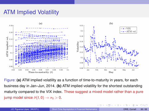
ATM Implied Volatility
Time-to-maturity (t)0.02 0.03 0.04 0.05 0.06 0.07 0.08 0.09 0.1
ATM
implied
vol.
0.06
0.08
0.1
0.12
0.14
0.16
0.18(a)
DayJan Feb Mar Apr May Jun
Volatility
0.06
0.08
0.1
0.12
0.14
0.16
0.18
0.2
0.22(b)
VIX
ATM vol.
Figure: (a) ATM implied volatility as a function of time-to-maturity in years, for each
business day in Jan–Jun, 2014. (b) ATM implied volatility for the shortest outstanding
maturity compared to the VIX index. These suggest a mixed model rather than a pure
jump model since σ(t , 0)→ σ0 > 0.
J.E. Figueroa-López (WUSTL) Short-Time Asymptotics in Financial Mathematics ORIE, Cornell 66 / 66


![Asymptotic Methods - Tartarus · of arg( z) is this approximation valid? [Hint: You may nd the substitution t = 2 1 useful. ] Paper 2, Section II 30A Asymptotic Methods (a) De ne](https://static.fdocuments.in/doc/165x107/5f3ec4f0b30bfe38ed1927e0/asymptotic-methods-tartarus-of-arg-z-is-this-approximation-valid-hint-you.jpg)


