SHORT-TERM RAIN PREDICTION WITH ARTIFICIAL NEURAL NETWORKS · SHORT-TERM RAIN PREDICTION WITH...

SHORT-TERM RAIN PREDICTION

WITH ARTIFICIAL NEURAL NETWORKS

A thesis submitted to the University of Manchesterfor the degree of Master of Science

in the Faculty of Science and Engineering

October 2000

ByAntonios Christofides

Department of Computer Science

Copyright c© 2000 Antonios Christofides

Copying (by any process), either in full or of extracts, is not allowed withoutprior written permission of the Author.

2

Contents

Abstract 7

Acknowledgements 9

About the author 11

1 Introduction 131.1 Forecasting and nowcasting . . . . . . . . . . . . . . . . . . . . . 131.2 Rain in the meteorological station of NTUA . . . . . . . . . . . . 141.3 Neural networks in meteorology and hydrology . . . . . . . . . . 16

2 Methodology 192.1 Patterns and pre-processing . . . . . . . . . . . . . . . . . . . . . 192.2 Pattern sets and error types . . . . . . . . . . . . . . . . . . . . . 212.3 Performance evaluation and baseline models . . . . . . . . . . . . 22

3 Experiments 253.1 Preliminary experiments . . . . . . . . . . . . . . . . . . . . . . . 253.2 Basic state prediction . . . . . . . . . . . . . . . . . . . . . . . . 273.3 Improved state prediction . . . . . . . . . . . . . . . . . . . . . . 30

4 Conclusions and further work 354.1 Conclusions . . . . . . . . . . . . . . . . . . . . . . . . . . . . . . 354.2 Additional results . . . . . . . . . . . . . . . . . . . . . . . . . . . 364.3 Further possibilities . . . . . . . . . . . . . . . . . . . . . . . . . 38

Appendix 39A.1 Perceptrons . . . . . . . . . . . . . . . . . . . . . . . . . . . . . . 39A.2 Simple networks . . . . . . . . . . . . . . . . . . . . . . . . . . . 40A.3 Sensitivity analysis for one hour prediction . . . . . . . . . . . . 40A.4 Radial basis networks . . . . . . . . . . . . . . . . . . . . . . . . 40A.5 One-hour value prediction . . . . . . . . . . . . . . . . . . . . . . 41A.6 Automatic relevance determination . . . . . . . . . . . . . . . . . 42

Bibliography 45

3

List of Tables

1.1 Weather conditions in Athens, Greece, for the period 1931–1990 . 15

2.1 Statistical characteristics of variables . . . . . . . . . . . . . . . . 212.2 Normalisation of variables . . . . . . . . . . . . . . . . . . . . . . 212.3 Distribution of rain patterns in months . . . . . . . . . . . . . . . 22

3.1 Patterns available for one hour prediction . . . . . . . . . . . . . 283.2 Performance of the no change baseline model for one hour prediction 283.3 Performance of feedforward networks for one hour prediction . . 293.4 Performance of the humidity-only model for one hour prediction 303.5 Patterns available for six hour prediction . . . . . . . . . . . . . . 313.6 Performance of feedforward networks for six hour prediction . . . 313.7 MAE of various sensitivity analysis models . . . . . . . . . . . . 323.8 Performance of the humidity-only model for six hour prediction . 323.9 Performance of NR-6-FF-5P . . . . . . . . . . . . . . . . . . . . . 33

4.1 Performance of NR-S-FF-5 with different thresholds . . . . . . . 37

A.2 Performance of baseline models . . . . . . . . . . . . . . . . . . . 39A.3 Performance of perceptrons . . . . . . . . . . . . . . . . . . . . . 40A.4 Performance of feedforward networks . . . . . . . . . . . . . . . . 40A.5 Performance of sensitivity analysis models for one hour prediction 41A.6 Performance of radial basis networks . . . . . . . . . . . . . . . . 41A.7 Standard error of the baseline models . . . . . . . . . . . . . . . 42A.8 Standard error of feedforward networks . . . . . . . . . . . . . . 42A.9 Results of ARD-10 . . . . . . . . . . . . . . . . . . . . . . . . . . 43A.10 Results of ARD-40 . . . . . . . . . . . . . . . . . . . . . . . . . . 44A.11 α for the various inputs for ARD-40 . . . . . . . . . . . . . . . . 44

4

List of Figures

3.1 Perc-30 training error . . . . . . . . . . . . . . . . . . . . . . . . 263.2 Different kinds of transfer functions . . . . . . . . . . . . . . . . . 263.3 FF-6 training error . . . . . . . . . . . . . . . . . . . . . . . . . . 27

4.1 Radial basis function in comparison to a logistic sigmoid . . . . . 37

5

Abstract

Virtually all research concerning short-term rain prediction to date makes useof spatial rainfall data, sometimes also taking another variable, such as winddirection, into account. This thesis explores the possibility of using neural net-works for short-term rain predictions from several meteorological variables fromonly one gauging station. The input variables examined, besides rainfall, arewind speed and direction, temperature, humidity, and barometric pressure. Themethod cannot compete with spatial methods, and the results are indeed im-practical, but they show some correlation which could be used to improve thespatial methods.

7

Acknowledgements

I would like to thank Dr. Jonathan Shapiro for his guidance and close supervi-sion. I would also like to thank Dr. Demetris Koutsoyiannis, Division of WaterResources, National Technical University of Athens, for his interest and his helpwith the meteorological part.

9

About the author

Antonios Christofides studied civil engineering at the National Technical Uni-versity of Athens (NTUA). He graduated in 1994, and since then he has been asystem administrator, web master, applications developer, and software engineerin various research programs undertaken by the Division of Water Resources,NTUA.

11

Chapter 1

Introduction

In this introduction the way long-term and short-term forecasts are carried outis presented; it is observed that all methods make use of spatial data, and that itmight be beneficial to study the problem with point data. The gauging stationwhose data have been used in the study, and the prevalent meteorological con-ditions and peculiarities of the site, are described. Finally, related works in theliterature are visited and the advantages of using neural networks are explained.

1.1 Forecasting and nowcasting

The foundation for modern meteorological prediction was laid by Richardson(1922), who built on the idea Vilhelm Bjerknes had published in 1904 of apply-ing the laws of motion and the laws of thermodynamics to weather prediction.Richardson devised methods of solving the equations using finite differences. Hedid not, however, have the means to make the required calculations, and al-though he had dreamt of a meteorological organisation where tens of thousandsof human computers would be making calculations in parallel, he had not antic-ipated the emergence of computing machines, which occurred two decades later.His work, forgotten in the meantime, was then revisited, and by the mid 1950scomputer-produced weather forecasts had become operational (Tribbia 1997).

For current global prediction, the finite difference method is applied on three-dimensional grids the nodes of which are at a distance of between one and twodegrees of latitude or longitude in the horizontal, and 500 and 1,000 m in thevertical direction (Tribbia 1997). For more accurate, local prediction, grids up tofour times more dense are used. Data are collected from fixed gauging stations,ships, aircraft, and meteorological balloons. The calculations are performedon computers which are among the most powerful in the world, consisting ofhundreds of parallel processors.

This huge process may be impressive and successful, but when it comes tovery-short-range predictions it doesn’t work. There is a significant delay inthe collection of data; meteorological balloons, in particular, are sent to theatmosphere for measurements only every 12 hours. In addition, the calculationstake several hour to complete. Finally, the forecasting models show instabilitiesand do not converge on the short term. Thus, even if the speed of calculations is

13

14 CHAPTER 1. INTRODUCTION

increased tenfold—a feat not at all unlikely for the next few years—this processwould not give us an answer to our short-range problem.

The techniques used in short-range forecasting are very different from theones mentioned above for medium and long-range forecasting; in fact, theyare often referred to with the distinct term nowcasting (Atkinson and Gadd1986, 126–128). Nowcasting actually refers to how the weather is now, whichis non-trivial to determine since there are gaps in the coverage of observingstations. Nowcasting is mainly achieved with weather radars and satellite im-ages. Weather radars trace clouds and rainfall, and can even estimate the rateof rainfall. Nowcasting techniques are also used for very-short-range forecastsby extrapolating the movement of cloud or rainfall patterns revealed either byDoppler radars or by sequences of radar or satellite images. An example of anowcasting application is a weather radar used by the BBC during the tennistournament at Wimbledon (Fox 1999).

Some experiments using artificial neural networks for short-term precipita-tion forecasting have also been performed. For example, Kuligowski and Bar-ros (1998) have created models that make predictions in the 0–6 hour rangefrom the measurements of numerous precipitation gauges and from wind direc-tion measurements.

All these methods, for either short- or medium- or long-range forecasts, makeuse of spatial data. The models developed in this project, however, use datafrom only one point; the measurements for a number of variables from a singlegauging station are used. This idea is not new; sea-weeds hung out of thewindow, man-made devices that change colour or have little people appear,dressed for rain or sunshine, and other simple means, have been used for centuriesas indications of the kind of weather to be expected; those methods are mostyindirect observations of humidity, some of them also taking barometric pressureinto account. Our models are, of course, more complex, making use of wind speedand direction, temperature, and rainfall, in addition to humidity and pressure,which are measured at a specific gauging station, and predict rain at that samepoint.

Neither can we compete with the spatial methods nor do we aspire to doso; nevertheless, it is interesting to explore what happens at a single point. Itmight turn out that there is more information at one point than we previouslythought, and other ways of exploiting that information could subsequently befound. The models developed have an error too large to be of any practical use,but still sufficiently small to show that there is indeed an interesting amount ofinformation at the site considered. What makes these results more important isthat rain at that site is an irregular and unpredictable phenomenon. The siteand this difficulty are presented in the following section.

1.2 Rain in the meteorological station of NTUA

The data used are from the Meteorological Station of the National Technical Uni-versity of Athens (NTUA). The station is described by Mamassis et al. (2000),

1.2. RAIN IN THE METEOROLOGICAL STATION OF NTUA 15

and also in the station’s web pages, http://www.hydro.ntua.gr/meteo/en/.1

It was installed in 1993 in the University Campus of NTUA at Zografou, Athens,Greece, about 4.5 km east of the centre of Athens, at the west feet of MountHymettus, one of the four mountains that surround Athens. It is fully auto-matic, logging the measurements of the sensors every ten minutes and trans-mitting them to the Hydraulics Building. The configuration of the station hasundergone changes during these seven years, but what matters here is that thereis a good, publicly available record of 10-minute measurements for the variablesof interest.2 In the models described in the following chapters, hourly valueshave been used.

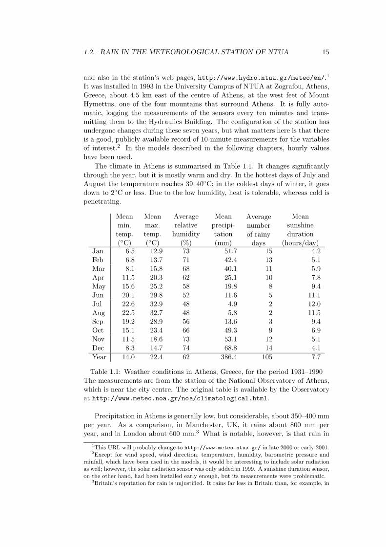
The climate in Athens is summarised in Table 1.1. It changes significantlythrough the year, but it is mostly warm and dry. In the hottest days of July andAugust the temperature reaches 39–40◦C; in the coldest days of winter, it goesdown to 2◦C or less. Due to the low humidity, heat is tolerable, whereas cold ispenetrating.

Meanmin.temp.(◦C)

Meanmax.temp.(◦C)

Averagerelative

humidity(%)

Meanprecipi-tation(mm)

Averagenumberof rainy

days

Meansunshineduration

(hours/day)Jan 6.5 12.9 73 51.7 15 4.2Feb 6.8 13.7 71 42.4 13 5.1Mar 8.1 15.8 68 40.1 11 5.9Apr 11.5 20.3 62 25.1 10 7.8May 15.6 25.2 58 19.8 8 9.4Jun 20.1 29.8 52 11.6 5 11.1Jul 22.6 32.9 48 4.9 2 12.0Aug 22.5 32.7 48 5.8 2 11.5Sep 19.2 28.9 56 13.6 3 9.4Oct 15.1 23.4 66 49.3 9 6.9Nov 11.5 18.6 73 53.1 12 5.1Dec 8.3 14.7 74 68.8 14 4.1Year 14.0 22.4 62 386.4 105 7.7

Table 1.1: Weather conditions in Athens, Greece, for the period 1931–1990The measurements are from the station of the National Observatory of Athens,which is near the city centre. The original table is available by the Observatoryat http://www.meteo.noa.gr/noa/climatological.html.

Precipitation in Athens is generally low, but considerable, about 350–400 mmper year. As a comparison, in Manchester, UK, it rains about 800 mm peryear, and in London about 600 mm.3 What is notable, however, is that rain in

1This URL will probably change to http://www.meteo.ntua.gr/ in late 2000 or early 2001.2Except for wind speed, wind direction, temperature, humidity, barometric pressure and

rainfall, which have been used in the models, it would be interesting to include solar radiationas well; however, the solar radiation sensor was only added in 1999. A sunshine duration sensor,on the other hand, had been installed early enough, but its measurements were problematic.

3Britain’s reputation for rain is unjustified. It rains far less in Britain than, for example, in


Athens varies highly with the season. The precipitation in June, July, Augustand September is next to negligible; the most rainy months are November andDecember, but close to them come October, January, February and March; andin April and May rainfall gradually decreases as summer approaches. In themost rainy month, December, it rains 14 times as much as it does in the driest,July; the equivalent factor in the UK is less than 2 in all locations. (Statisticalmeteorological data for the UK is available by the UK Meteorological Office,http://www.met-office.gov.uk/ukclimate/averages_sites.html.)

There are about 100 rainy days in the year, i.e. 27%. Here, however, we areworking on an hourly basis. In the rainy days, it usually rains only for a fewhours in the day. As a result, in the 8,760 hours of the year, there are only about250 rainy hours, i.e. 3%. For many days, or weeks, rain can stay at zero, thenrise to some nonzero value. These sudden changes are difficult to predict, andmake the problem especially challenging.

1.3 Neural networks in meteorology and hydrology

Since the publication of Parallel Distributed Processing by D. E. Rumelhart andJ. L. McClelland in 1986, which is considered to mark the beginning of thenew connectionist era, the capabilities of artificial neural networks have beenexplored in all sciences, meteorology and hydrology being no exception. Thework by Kuligowski and Barros (1998) has already been mentioned. There area number of other works, of which a sample of the most recent will be presentedhere.

Khotanzad et al. (1996) have developed a model that predicts the hourlytime series of temperature for the next seven days. The inputs to the model arethe hourly time series of the previous day and the weather service’s predictionsfor high and low temperatures for the days to be forecast. This system, whichthey claim to be of particular interest to electric companies, can hardly be said tobe really a forecaster, as the most important part of the job, i.e. the predictionof the temperature extremes, has already been done by the weather service.However, the work demonstrates a simple meteorological application of neuralnetworks.4

River level and discharge are of great interest in hydrology, since water fromrivers is used in such activities as irrigation and power production, and becausefloods can cause damage to property or even deaths. Thus, the prediction ofriver level occupies a large part of the literature. See and Openshaw (1999), forexample, have attempted to enhance flood forecasting by using a combinationof soft modelling techniques, namely neural networks, fuzzy logic, and geneticalgorithms. The input to their overall system is the current river level andrainfall time series. The output of each part of the model is fed into the nextpart, the overall output being an estimation of the danger of flooding. A number

western Greece, where the annual rainfall exceeds 1,200 mm.4Throughout this text, the term “neural network” is used where the more accurate “artificial

neural network” is intended. This clarification is necessary because artificial neural networks,though having largely been inspired by their biological counterparts, have very little in commonwith them.

1.3. NEURAL NETWORKS IN METEOROLOGY AND HYDROLOGY 17

of works, such as that by Atiya et al. (1999) concern the River Nile, for whichlonger-term forecasts, such as for a month ahead, are interesting; the Nile’s flowis predictable on the short term, whereas it is Egypt’s only source of water,making long-term predictions especially important.

What has made neural networks largely successful in this area is that hydro-logical and meteorological phenomena are very complex. Neural networks, whilebeing essentially simple, are capable of implementing extremely complex input-output mappings; the work by Lapedes and Farber (1988) provides a simpletheoretical explanation for this capability. Techniques such as the backpropaga-tion algorithm enable the models to detect the relation between input and outputand thus automatically estimate the parameters, a process which is designatedby the occasionally confusing terms training and learning. Thus, in many casesneural networks are appropriate for modelling phenomena of great complexity.

The traditional simple devices that are used to indicate weather make verysimple mappings. If humidity is high, or if barometric pressure is low, theprobability of rain is higher. Although this may be correct, it rarely works inpractice. There may, however, be more knowledge in more variables. It mightbe, for example, that a drop in pressure, accompanied by a drop in temperatureand a certain change in wind speed and direction, constitute a “signature” ofimpending rain. In this work, we try to have neural networks determine whethersuch a signature exists and recognise it. Rain has been chosen as the outputvariable, because the prediction of rain is the most interesting and probably themost useful.

Chapter 2

Methodology

In this chapter essential background that underlies all experiments of the follow-ing chapters is given. The input and output of the models is explained, as wellas the various data sets. An overview of the way performance is evaluated andof the baseline models that are used as reference is also presented.

2.1 Patterns and pre-processing

A number of experiments will be presented in the following chapter. Each ex-periment uses a set of patterns, each pattern being a set of values. For example,in most experiments the pattern consists of six real input values (temperature,humidity, barometric pressure, rainfall, and two co-ordinates of wind vector)and one binary output value (whether it will rain or not). Not all experimentsmake use of the same data. A general description of the patterns follows, andthe specific details of each experiment are mentioned later.

There is always one output value, which may be either the quantity of rain inthe next hour, or a binary value, 1 or 0, standing for nonzero or zero rain in thenext one or six hours. The number of input values depends on the model, butgenerally it is the last few measurements of wind vector, temperature, humidity,barometric pressure, and rain. In most cases, the last hourly value is used.In some experiments, the values for the previous hours are used as well. Ten-minute measurements have also been attempted, and the effects of using thecurrent time and season have also been examined.

In theory, a neural network with an adequate number of hidden layers andnodes can perform any kind of mapping between the input and output variables.In most cases, however, some pre-processing of the input is necessary. Chapter 8of Bishop (1995) explains in detail why this is the case; the basic idea is that withpre-processing we can incorporate some prior knowledge in the input, which maybe very hard for the model to determine. In our case, pre-processing involvesthe following procedures:

• The transformation of wind speed and direction, in other words of thepolar co-ordinates of the wind vector, into Cartesian co-ordinates.

• The substitution of the co-ordinates of a unit vector in place of current

19

20 CHAPTER 2. METHODOLOGY

time and current season.

• The normalisation of variables.

The original wind variables are wind speed and wind direction. Wind direc-tion is given in degrees, where 0 is north and 90 is east. Wind direction is highlynonlinear, its problem being the discontinuity at the north; a wind direction of359◦ is pretty much the same as 0◦. Using Cartesian co-ordinates in place of thewind speed s and the wind direction φ is better, since Cartesian co-ordinates arecontinuous. The x direction is defined as east-west, where positive is east, andy as north-south, where positive is south. The conversion is done as follows:

x = −s sin φ

y = −s cos φ

A similar problem exists in the representation of the time of day. If, forexample, the number of minutes since midnight is used, then there is a discon-tinuity at midnight, where from 1439 minutes we jump back to 0. The solutionis to arrange the hours in a circle with unit radius, like a 24-hour clock, with 0hours at the top and then clockwise from 1 through 23, and use the Cartesianco-ordinates of the vector that points to the current time. If t is the currentminute of day, then these co-ordinates are:

x = sin(t/1440× 2π)y = cos(t/1440× 2π)

Likewise, the season is the number of month, from 1 to 12. If months arearranged like a 12-hour clock, the co-ordinates of month m are

x = sin(m/12× 2π)y = cos(m/12× 2π)

Normalisation has been done so that the values of the variables are in the(0, 1) range, except for the wind co-ordinates, the normalised values of whichare in the (–1, 1) range. If m is the minimum value of a variable x, and m + ris the maximum (r is the range), then the normalised value may be defined as(x−m)/r. Usually we use a somewhat smaller, rounded value in place of m, anda larger, rounded value in place of r. In all cases, normalisation is virtually achange in the unit of measurement, and is thus certain not to have any unwantedeffects. For the wind co-ordinates, a different sign indicates an opposite direction,and thus the sign has been preserved after normalising, making the normalisedco-ordinates being in the (–1, 1) range. The minimum and maximum valuesof the variables in their original units, together with some other statistics, areshown in Table 2.1. The values have been normalised as shown in Table 2.2.The co-ordinates of the unit time and season vectors have been left as they are,in the (–1, 1) range.

2.2. PATTERN SETS AND ERROR TYPES 21

Variable Unit Minimum Maximum Mean St. devWind x m/s −8.2 8.1 −0.3 1.5Wind y m/s −11.5 10.5 −0.6 2.9Temperature ◦C −1.5 41.8 16.6 7.5Humidity % 13.7 98.6 58.5 17.4Barom. pressure hPa 960.2 1007.1 989.3 5.7Rainfall mm 0 38.5 0.05 0.66Nonzero rainfall mm 0.1 38.5 1.79 3.48

Table 2.1: Statistical characteristics of variables(on an hourly basis)

Variable How normalisedWind component x/40Temperature (x + 5)/50Humidity x/100Barom. pressure (x− 960)/50Rainfall x/100

Table 2.2: Normalisation of variables

2.2 Pattern sets and error types

The six years of measurements available, excluding some periods of malfunction,allow for a data set of about 40,000 patterns. This will be named the entirepattern set. The future value of rain (that of the next hour) is zero in most ofthese patterns, being it nonzero in only 1,138 patterns.

Since the entire pattern set is heavily biased towards zero rain, the reducedpattern set is usually used. The definition of the reduced pattern set differsfrom experiment to experiment, but it generally consists of the 1,138 nonzerorain patterns plus a randomly selected sample of 1 or 2 thousand zero rainpatterns. Since the distribution of rain is not uniform through the year, therandom selection of the patterns with zero rain must not be uniform either. Theactual distribution of rain is shown in Table 2.3. The selection of the zero rainpatterns that are included in the reduced pattern set is made at random, butfollowing that distribution.

The reduced pattern set is partitioned into a training set and a validationset, usually by dividing into halves or thirds (one third for training and two forvalidation).

The way performance is evaluated is discussed in detail in Section 2.3 below,but evaluation is generally based on the mean absolute or square error. Accord-ing to the pattern set on which they are measured, error figures are divided intothe following categories:

Training error This is the error measured on the training set, typically duringtraining.

Validation error It is measured after training, on the validation set.


Number of patternsJan 199Feb 90Mar 170Apr 94May 59Jun 10Jul 5Aug 18Sep 20Oct 81Nov 101Dec 291

Table 2.3: Distribution of rain patterns in months

Test error The entire pattern set has different characteristics than the reduced,thus it is important to measure performance on that as well; the resultingfigure is called the test error. In some models, the test error is measuredonly on a subset of (e.g. half) the entire pattern set, the rest of it being usedto determine some parameters (e.g. the ratio of nonzero to zero rainfall).

2.3 Performance evaluation and baseline models

When the model predicts state, i.e. 1 for a prediction of rain and 0 for a predictionof no rain, the mean absolute error, or MAE, is used for evaluating performance:

MAE =1n

n∑i=1

|ti − oi|

where n is the size of the data set, oi is the output of the model and ti is thetarget output; ti and oi have a value of 1 or 0. Depending on the type of error,the data set can be the entire (or part of), validation, or training, as describedin the previous section.

For models that predict value, i.e. a prediction of the rainfall depth, the meansquare error, or MSE, is used:

MSE =1n

n∑i=1

(ti − oi)2

where, this time, ti and oi are real values. The square root of the MSE is thestandard error. The standard error is usually denormalised, so that its units ofmeasurements are the original, i.e. mm of rain.

The mean absolute and mean square error, however, are not adequate indi-cators. One of the oldest known misuses of the mean absolute error occurredin 1884 (Murphy 1997), when J. P. Finley, while making similar experiments,determined the mean absolute error of his forecasts of tornadoes or no tornadoes

2.3. PERFORMANCE EVALUATION AND BASELINE MODELS 23

to be 3.4%; it was soon pointed out that a baseline model always predicting notornadoes produced an error of only 1.8%. It is thus important to interpret theMAE and MSE only in reference to the errors of baseline models.

Different baseline models are specified for different experiments, but the typesof baseline models are generally the following:

No change This model predicts that it will rain if and only if it currentlyrains; or that the amount of rain in the next hour equals the amount inthe previous hour. This is the baseline model that performs best in mostcases.

Zero rain This model always predicts no rain.

Rain This is the opposite of the zero rain model; it always predicts rain. It isused only when predicting state.

Random The prediction of rain at random is performed by assigning a proba-bility of rain equal to the ratio of rain to no rain outputs in the data set.Also used for state predictions only.

Average It is used only when predicting value, and makes a prediction equalto the expected value of rain. It is very much like the zero rain model,but it should perform somewhat better, since the mean value minimisesthe MSE. The prediction of this model is different for the validation andthe test sets; expected value of rain is 0.6 mm for the validation set and0.05 mm for the entire set.

Chapter 3

Experiments

There are two possible kinds of experiments: (a) State prediction, that is, modelsthat predict whether it is going to rain or not, regardless of the rainfall depth;(b) Value prediction, that is, models that predict the rainfall depth. The latteris only mentioned in the Appendix, as most experiments have been with state.These are presented in this chapter. First, some preliminary experiments arediscussed where state is predicted for the hour that follows. These are refinedin some significant details in the next section. After that we deal with stateprediction for six hours.

3.1 Preliminary experiments

A number of experiments have been performed initially, with generally poorresults. They are briefly mentioned here for completeness, although most of theoutcomes of the experiments are tabulated in the Appendix.

3.1.1 Perceptrons

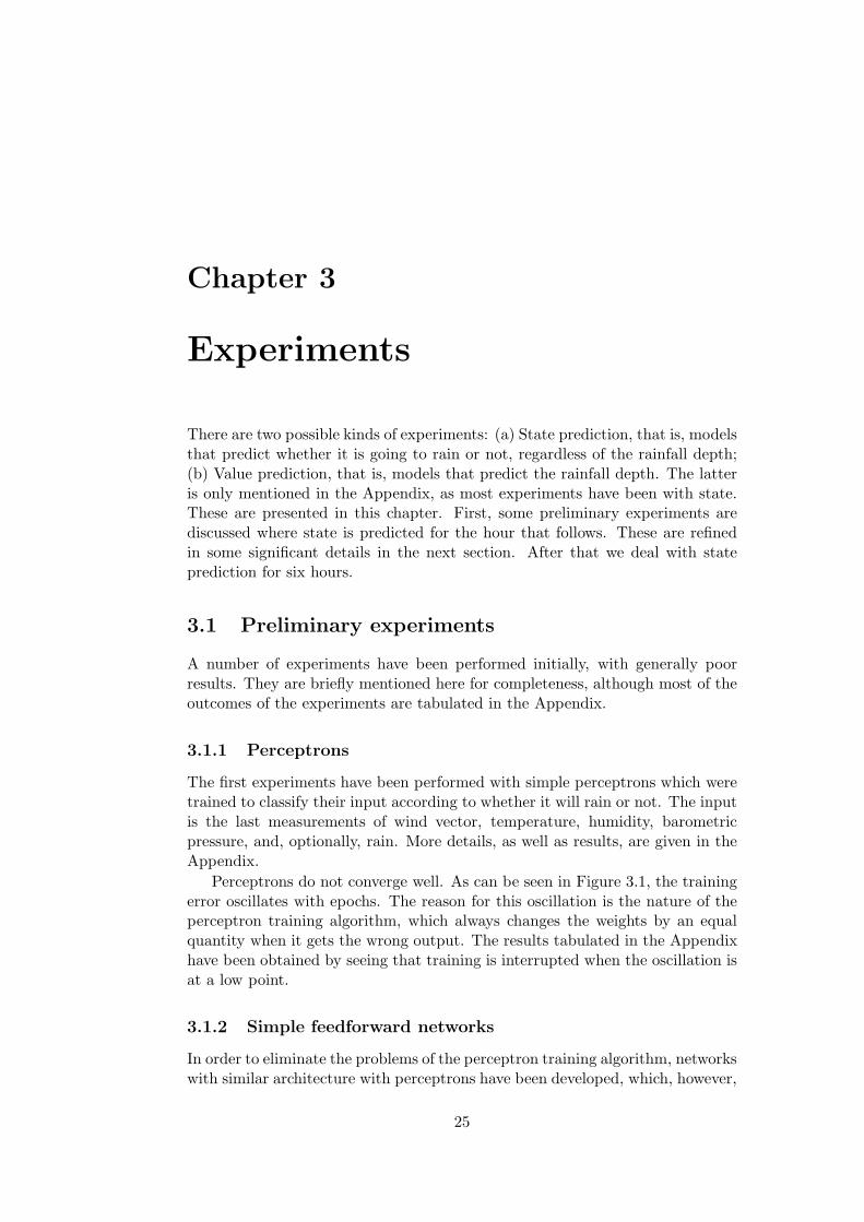
The first experiments have been performed with simple perceptrons which weretrained to classify their input according to whether it will rain or not. The inputis the last measurements of wind vector, temperature, humidity, barometricpressure, and, optionally, rain. More details, as well as results, are given in theAppendix.

Perceptrons do not converge well. As can be seen in Figure 3.1, the trainingerror oscillates with epochs. The reason for this oscillation is the nature of theperceptron training algorithm, which always changes the weights by an equalquantity when it gets the wrong output. The results tabulated in the Appendixhave been obtained by seeing that training is interrupted when the oscillation isat a low point.

3.1.2 Simple feedforward networks

In order to eliminate the problems of the perceptron training algorithm, networkswith similar architecture with perceptrons have been developed, which, however,

25

26 CHAPTER 3. EXPERIMENTS

0 100 200 300 400 500 600 700 800 90010

-1

100

Performance is 0.247059, Goal is 0

990 Epochs

Tra

inin

g-B

lue

Figure 3.1: Perc-30 training error

instead of a hard limiting transfer function, use the logistic sigmoid:

logsig(x) =1

1 + e−x

The shape of this function is shown in Figure 3.2 in comparison to a hard limitingfunction. The use of a continuous function makes possible the use of a gradientdescent training algorithm.

-1 -0.5 0 0.5 1

0

0.5

1

(a) Hard limiting

-5 0 5

0

0.5

1

(b) Logistic sigmoid

Figure 3.2: Different kinds of transfer functions

The output of the transfer function is between 0 and 1 exclusive. Duringtraining, the extreme values of 1 and 0, standing for rain and no rain, are stillgiven as target outputs. During simulation, the output of the sigmoid functionhas to be passed through a hard limiting function. An initial choice for thethreshold could be 0.5. Alternatively, the threshold can be specified so that

3.2. BASIC STATE PREDICTION 27

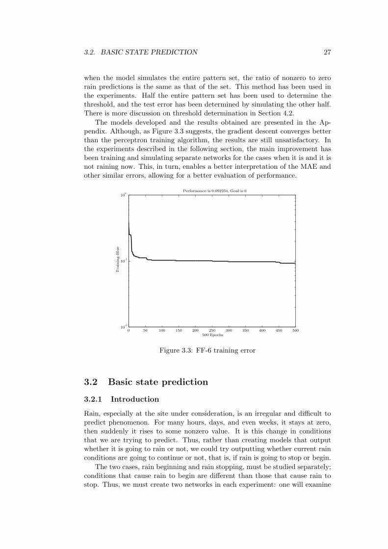
when the model simulates the entire pattern set, the ratio of nonzero to zerorain predictions is the same as that of the set. This method has been used inthe experiments. Half the entire pattern set has been used to determine thethreshold, and the test error has been determined by simulating the other half.There is more discussion on threshold determination in Section 4.2.

The models developed and the results obtained are presented in the Ap-pendix. Although, as Figure 3.3 suggests, the gradient descent converges betterthan the perceptron training algorithm, the results are still unsatisfactory. Inthe experiments described in the following section, the main improvement hasbeen training and simulating separate networks for the cases when it is and it isnot raining now. This, in turn, enables a better interpretation of the MAE andother similar errors, allowing for a better evaluation of performance.

0 50 100 150 200 250 300 350 400 450 50010

-2

10-1

100

Performance is 0.092234, Goal is 0

500 Epochs

Tra

inin

g-B

lue

Figure 3.3: FF-6 training error

3.2 Basic state prediction

3.2.1 Introduction

Rain, especially at the site under consideration, is an irregular and difficult topredict phenomenon. For many hours, days, and even weeks, it stays at zero,then suddenly it rises to some nonzero value. It is this change in conditionsthat we are trying to predict. Thus, rather than creating models that outputwhether it is going to rain or not, we could try outputting whether current rainconditions are going to continue or not, that is, if rain is going to stop or begin.

The two cases, rain beginning and rain stopping, must be studied separately;conditions that cause rain to begin are different than those that cause rain tostop. Thus, we must create two networks in each experiment: one will examine


the situation when it is not raining, predicting whether rain is going to begin ornot; the other will examine the situation when it is raining, predicting whetherrain is going to stop or not. The networks, pattern sets, etc., that have to dowith these two cases will be denoted by NR and R respectively.

We now observe that, having divided the problem in these two subproblemsto be studied separately, there is no difference as to whether we predict rain orchange. In the R case, a prediction of rain is a prediction of no change, andvice-versa; in the NR case, predicting rain and change are identical. Thus, theimportant step is to recognise the necessity of distinguishing cases R and NR;we will continue to use output 1 for rain and 0 for no rain.

3.2.2 Pattern sets and error types

The number of patterns available is shown in Table 3.1.

Now raining Now not rainingWill rain 723 415 1,138Will not rain 419 38,154 38,573

1,142 38,569 39,711

Table 3.1: Patterns available for one hour prediction

The R-entire set will be the 1,142 patterns in which it is currently raining;the NR-entire set will be the 38,569 patterns in which it is currently not raining.The R-reduced pattern set will be the same as the R-entire set; the NR-reducedset will be the 415 patterns in which rain is going to begin plus twice as many(830) patterns in which it continues not to rain. These 830 patterns are chosenat random among the 38,154 available, but with the same distribution throughthe year as the 415 involving change. In both cases, R and NR, the reducedpattern set will usually be divided into a training set and a validation set. TheMAE on these sets will be named the training and the validation error. TheMAE on the NR-entire set will be the test error. There will be no such errorfor the R case (or it will be considered the same as the validation error), due toinsufficient number of available data.

The R-no-change model is the same as the R-rain model; the NR-no-changemodel is the same as the NR-no-rain model. Since in both cases the no changemodel performs better than the alternative, this will be used as the baselinemodel in all cases. The performance of this model is shown in Table 3.2.

Validation error Test errorR 0.37 (0.37)NR 0.33 0.01

Table 3.2: Performance of the no change baseline model for one hour prediction

3.2.3 Simple feedforward networks

The following models have been attempted:

3.2. BASIC STATE PREDICTION 29

R-FF-6 This is a one layer feedforward network with 6 inputs and 1 output.Its inputs are the last hourly measurement of wind vector, temperature,humidity, barometric pressure, and rain. Its output, a sigmoid passedthrough a thresholding function, is 1 for a prediction of rain and 0 oth-erwise. R-FF-6 is only trained and simulated with the R-pattern sets,patterns in which the last measurement of rain is nonzero.

NR-FF-5 This is almost identical to R-FF-6, but it is trained and simulatedwith the NR-pattern sets, the patterns of which always have a zero currentrainfall. Since this is always zero, there is no point in including it as aninput, thus NR-FF-5 only has 5 inputs.

Results are shown in Table 3.3.

R-no-change R-FF-6 NR-no-change NR-FF-5Threshold 0.56 0.85Training error 0.22 0.15Validation error 0.37 0.31 0.33 0.32Valid. err. given will rain 0 0.15 1 0.94Valid. err. giv. won’t rain 1 0.57 0 0.016Test error 0.011 0.016Test error given will rain 1 0.94Test error giv. won’t rain 0 0.007No rain given pred. rain 0.92

Table 3.3: Performance of feedforward networks for one hour predictionThese results are an indication, as different results are obtained each time themodels are run.The last row of the table is the probability that it will not rain given that themodel predicted it will rain. In other words, if the test error given it will rain isP(P|R), then the last row of the table gives P(R|P).

We can see that R-FF-6 performs somewhat better than the baseline model,but not significantly so. For the more difficult and challenging case of NR, wesee that NR-FF-5 performs interestingly in the validation set. In the test set,its overall performance is significantly worse than that of the baseline model,with an error of 1.6% instead of 1.1%. However, the conditional errors for thecases where it is or is not going to rain deserve more attention. For those cases,the baseline model tells us nothing. A random model, on the other hand, whichwould predict rain with a probability of 1.1%, would have an error of 1.1% givenit will not rain and 98.9% given it will rain; this performance is worse than thatof NR-FF-5.

We see, however, that the numbers are very small, because the data arenot enough for more detailed analysis. Rain is a rare phenomenon. We mayhave 40,000 patterns in total, but only 1140 involve rain, and of those 415only are changes from no rain to rain. A possible next step in our attempt toimprove model performance could be to create a seasonal model, that is, dividethe year into seasons (e.g. into 12 months) and use a different model for each


one. Conditions that cause rain to begin may be different in winter than in thesummer, and a seasonal model might be able to account for those differences.However, it is not possible to do any further analysis in our case, since a seasonalmodel would mean using an even smaller sample. On the other hand, the patternset we have used so far is strongly biased towards winter, and a seasonal modelmight not make much difference.

In the following section, a closer examination of the above results revealsadditional problems. Some improvements to the models are also suggested andattempted.

3.3 Improved state prediction

3.3.1 Sensitivity analysis

Sensitivity analysis has been performed in order to determine the effect of eachindividual variable on the prediction of NR-FF-5. There are a number of waysto perform sensitivity analysis, of which a simple one has been followed: 5 newmodels have been created, almost alike NR-FF-5, but with one of the inputvariables missing in each one.

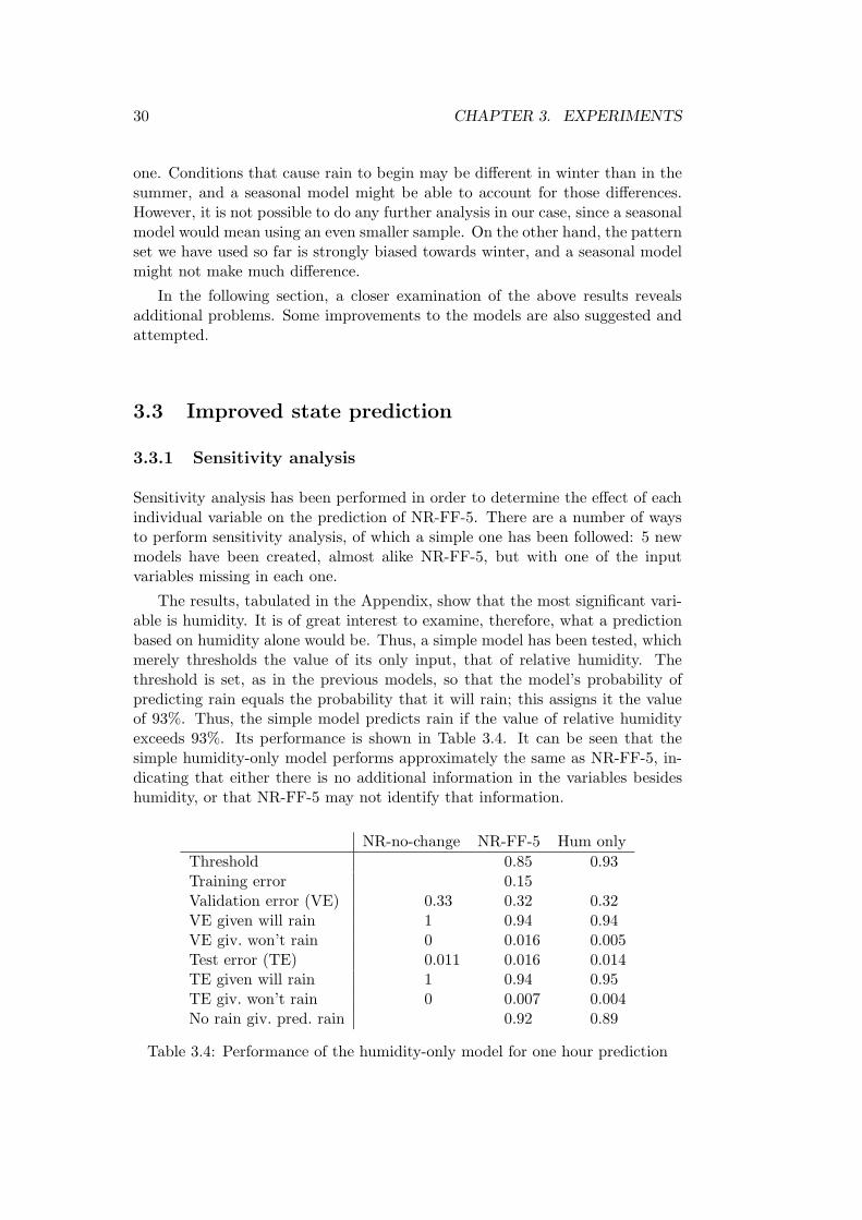
The results, tabulated in the Appendix, show that the most significant vari-able is humidity. It is of great interest to examine, therefore, what a predictionbased on humidity alone would be. Thus, a simple model has been tested, whichmerely thresholds the value of its only input, that of relative humidity. Thethreshold is set, as in the previous models, so that the model’s probability ofpredicting rain equals the probability that it will rain; this assigns it the valueof 93%. Thus, the simple model predicts rain if the value of relative humidityexceeds 93%. Its performance is shown in Table 3.4. It can be seen that thesimple humidity-only model performs approximately the same as NR-FF-5, in-dicating that either there is no additional information in the variables besideshumidity, or that NR-FF-5 may not identify that information.

NR-no-change NR-FF-5 Hum onlyThreshold 0.85 0.93Training error 0.15Validation error (VE) 0.33 0.32 0.32VE given will rain 1 0.94 0.94VE giv. won’t rain 0 0.016 0.005Test error (TE) 0.011 0.016 0.014TE given will rain 1 0.94 0.95TE giv. won’t rain 0 0.007 0.004No rain giv. pred. rain 0.92 0.89

Table 3.4: Performance of the humidity-only model for one hour prediction

3.3. IMPROVED STATE PREDICTION 31

3.3.2 Six-hour state prediction

The results obtained so far suggest that it is not possible to get any reasonableperformance when trying to predict one hour ahead. The possibility of improvingperformance by adding hidden layers or adjusting the threshold differently isdiscussed in Chapter 4, but no substantial improvement has been achieved.

The poor performance may be due to an inherent degree of unpredictabilityof rainfall. In the experiments presented above, we have asked the models notonly to recognise rainy situations, but to predict exactly the hour in which therain is going to begin. This task, challenging even for radars, has proven toverge on the impossible for our models. In the experiments presented below, therules have been relaxed and the models are now asked to make a more generalprediction, for the next 6 hours. The output of the NR models is now 1 or 0standing for whether it is going to begin to rain or not sometime within the next6 hours; this means that the models are asked to recognise rainy conditions, butnot the exact hour of rainfall.

The number of patterns available is shown in Table 3.5.

Now raining Now not rainingWill rain 889 1,735 2,624Will not rain 229 35,919 36,148

1,118 37,654 38,772

Table 3.5: Patterns available for six hour prediction

The main model developed is denoted NR-6-FF-5; it is identical with NR-FF-5, only it is trained and tested with the new pattern sets. Results are shownin Table 3.6.

NR-6-no-change NR-6-FF-5Threshold 0.65Training error 0.18Validation error 0.35 0.31Valid. err. given will rain 1 0.83Valid. err. giv. won’t rain 0 0.042Test error 0.045 0.059Test error given will rain 1 0.85Test error giv. won’t rain 0 0.021No rain giv. pred. rain 0.75

Table 3.6: Performance of feedforward networks for six hour predictionThese results are an indication, as different results are obtained each time themodels are run. The validation error of NR-no-change, in particular, is expectedto be 0.33; however, it happened to be 0.35 on that particular validation set.The NR-6-FF-5 values shown for comparison have been determined on exactlythe same sets.

Sensitivity analysis has been performed as described above; results are shownin Table 3.7.


Variable missingNR-6-FF-5 Wind x Wind y Tem Hum Pres

Threshold 0.65 0.65 0.63 0.65 0.62 0.55Training error 0.18 0.18 0.18 0.18 0.19 0.20Validation error (VE) 0.31 0.32 0.31 0.32 0.32 0.33VE given will rain 0.83 0.84 0.84 0.84 0.84 0.89VE giv. won’t rain 0.042 0.042 0.038 0.043 0.052 0.029Test error (TE) 0.059 0.060 0.060 0.060 0.078 0.057TE given will rain 0.85 0.86 0.86 0.86 0.85 0.90TE giv. won’t rain 0.021 0.022 0.021 0.022 0.030 0.017No rain giv. pred. rain 0.75 0.77 0.77 0.77 0.81 0.77

Table 3.7: MAE of various sensitivity analysis models

A simple humidity model has also been tested, and its results are shownin Table 3.8. In this 6 hour prediction, our neural network seems to performslightly better than the humidity only model.

NR-6-no-change NR-6-FF-5 Hum onlyThreshold 0.65 0.87Training error 0.18Validation error (VE) 0.35 0.31 0.33VE given will rain 1 0.83 0.88VE giv. won’t rain 0 0.042 0.040Test error (TE) 0.045 0.059 0.059TE given will rain 1 0.85 0.90TE giv. won’t rain 0 0.021 0.019No rain giv. pred. rain 0.75 0.79

Table 3.8: Performance of the humidity-only model for six hour prediction

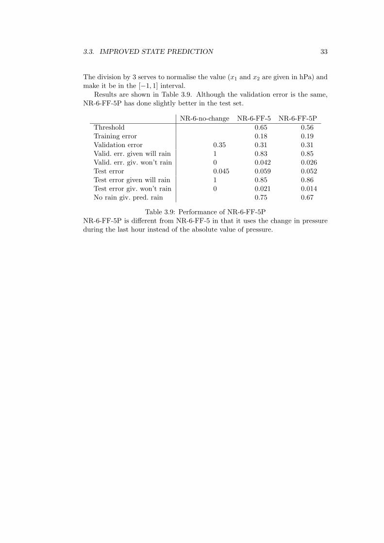
3.3.3 Using the change in pressure

Barometric pressure is a relative quantity. The average barometric pressure atsea level is 1,015 hPa, but if the pressure at a certain point is lower than average,and the pressure around that point is even lower, then that point is considered ahigh pressure. Our models cannot know whether the point considered is a highor a low pressure, since there is no spatial data available. However, it may besignificantly more informative to know what the change in pressure has beenduring the last hour, than the absolute value of pressure.

Model NR-6-FF-5P has thus been developed, which is identical to NR-6-FF-5, the only difference being that the barometric pressure input has been substi-tuted by the change in pressure. If x1 and x2 are the last and the last but onehourly measurements of barometric pressure, then the input under considerationis

(x1 − x2)/3

3.3. IMPROVED STATE PREDICTION 33

The division by 3 serves to normalise the value (x1 and x2 are given in hPa) andmake it be in the [−1, 1] interval.

Results are shown in Table 3.9. Although the validation error is the same,NR-6-FF-5P has done slightly better in the test set.

NR-6-no-change NR-6-FF-5 NR-6-FF-5PThreshold 0.65 0.56Training error 0.18 0.19Validation error 0.35 0.31 0.31Valid. err. given will rain 1 0.83 0.85Valid. err. giv. won’t rain 0 0.042 0.026Test error 0.045 0.059 0.052Test error given will rain 1 0.85 0.86Test error giv. won’t rain 0 0.021 0.014No rain giv. pred. rain 0.75 0.67

Table 3.9: Performance of NR-6-FF-5PNR-6-FF-5P is different from NR-6-FF-5 in that it uses the change in pressureduring the last hour instead of the absolute value of pressure.

Chapter 4

Conclusions and further work

Some conclusions have already been mentioned in the previous chapters; themain points are recapitulated here. Some less important, additional experimentsthat have been made are discussed, leading the way into suggestions for furtherresearch possibilities.

4.1 Conclusions

The main conclusions of the experiments are the following:

• It seems preferable to divide the pattern set into those patterns where thelast measurement of rain is zero and those where it is nonzero, and totrain different networks for each case. It is thus predicted whether rain isgoing to begin or stop, rather than whether it is going to rain or not. Inthe models developed, this improves the results. It also makes the errorfigures provide greater insight.

• In the case when it is not currently raining, humidity is the variable towhich the models developed are most sensitive.

• In predictions of whether rain will begin within an hour, the neural net-works developed do not perform any better than a simple humidity-onlymodel. It is likely that this situation cannot improve considerably by elab-orating the models, since rainfall is a phenomenon with an inherent degreeof unpredictability.

• In predictions of whether rain will begin within six hours, the models devel-oped seem to perform better than the baseline, but only in the validationset.

• Pressure change is probably more important than the absolute value ofpressure.

• The main constraint is the lack of data. Increasing the model complexityby adding hidden layers or by taking more inputs into account, such as10-minute data or more previous measurements, is hardly possible, as the

35

36 CHAPTER 4. CONCLUSIONS AND FURTHER WORK

amount of data does not allow for a significant increase in the degrees offreedom. Unfortunately, there are very few sites in Greece with a goodrecord of measurements for some decades, which would be necessary forfurther investigation.

The error figures may seem discouraging, but, as stated in the Introduction,our aim is not so much to get good results, which would certainly be inferiorto those of existing nowcasting methods, but rather to explore the amount ofinformation in our single point of interest. In addition, we have made thingsgradually more difficult, by setting up baseline models which, though essentiallytelling nothing, have a very low error. At the site under consideration it rarelyrains, thus it is extremely hard to outperform a baseline model that predictsthat it never rains. And yet, when our models indicated, by means of sensitivityanalysis, that humidity is the most important variable, the simple humidity-onlymodel was set up, which is even harder to beat. It remains true, however, thatthe models, in their present form, are of little practical value. Some suggestionsfor improvement are made in the following sections.

4.2 Additional results

4.2.1 Hidden layers

It has been attempted to add hidden layers to models such as NR-FF-5 and NR-S-FF-5P. It has been found that some configurations, such two hidden layerswith 3 and 2 nodes, may have some effect on the result, but at present this effectis very small and does not justify the greater model complexity.

4.2.2 Radial basis networks

Different network architectures are interesting alternatives. Radial basis net-works, in particular, have some benefits; they have one hidden layer the nodesof which use a radial basis transfer function, usually of the following form:

f(x) = e−x2

A plot of this function is shown in Figure 4.1. The main feature of such anode is that it gives a high output whenever its inputs are close to a “perfect”pattern; the output quickly drops to zero at both directions. In contrast, alogistic sigmoid transfer function constantly increases in one direction.

An experiment with radial basis networks has been attempted. Its results,tabulated in the Appendix (Table A.6), are comparable to those of NR-FF-5.

4.2.3 Thresholds

As has already been mentioned, the threshold of any model is determined sothat the ratio of nonzero to zero rain predictions is the same as the probabilityof rain. Though this way of determination is simple and reasonable, there isno compelling why it should necessarily be so. An alternative which has been

4.2. ADDITIONAL RESULTS 37

-2 0 2

0

0.5

1

(a) Radial basis

-5 0 5

0

0.5

1

(b) Logistic sigmoid

Figure 4.1: Radial basis function in comparison to a logistic sigmoid

attempted is to set the threshold so that the error is minimised. Table 4.1 showssome results. As can be seen, minimising the test error almost reduces the modelto the baseline which predicts that it never rains. Minimising the validation errorincreases the test error.

What is minimisedNR-S-FF-5 Validation error Test error

Threshold 0.65 0.43 0.94Validation error 0.31 0.27 0.35Valid. err. given will rain 0.83 0.57 0.997Valid. err. giv. won’t rain 0.042 0.115 0Test error 0.059 0.108 0.045Test error given will rain 0.85 0.60 0.996Test error giv. won’t rain 0.021 0.085 0.0001No rain giv. pred. rain 0.75 0.81 0.40

Table 4.1: Performance of NR-S-FF-5 with different thresholds

4.2.4 Automatic relevance determination

The technique of automatic relevance determination has been attempted as analternative to sensitivity analysis; this is discussed extensively in the Appendix.It has been concluded that this technique does not work well, its main problembeing that it does not account for correlations between the input variables.

4.2.5 Value prediction

In all experiments mentioned so far we have made a distinction between caseswhen it rains and cases when it does not rain, implying that these cases are clear-cut. However, there is a degree of fuziness in the concept of precipitation. Anyrainfall sensor or gauge has a resolution, and the particular sensor used in NTUAhas a resolution of 0.1 mm. Thus, a measurement of zero does not necessarilymean no rain; it might be 0.05 mm. The slight fuziness does not, however,depend only on sensor accuracy, but is natural. A rainfall rate of 0.1 mm per

38 CHAPTER 4. CONCLUSIONS AND FURTHER WORK

hour would probably not affect any human action, and no-one would botheropening their umbrella, so such a rate can hardly be classified as rain. In fact,whether a certain intensity is classified as rain or not depends on the reasonfor which we use this information. An intensity of 0.1 mm per hour is a verydifferent thing, and a very different phenomenon, than an intensity of 50 mmper hour, which is heavy rain. And yet, in all models examined so far, we havetreated both these values as a mere “yes”, as opposed to 0, “no”, without makingany distinction.

The obvious way to predict the amount, rather than the possibility, of rain,is to remove the hard-limiting function, using the output of the sigmoid func-tion, and train the network with real rather than boolean values. A few suchexperiments have been performed, and are presented in the Appendix, but theirresults are poor. It is, however, a matter most worth of further investigation.

4.3 Further possibilities

Except for alternative network architectures, different ways of determining thresh-olds, and making a value rather than a state prediction, which have all beendiscussed in the previous section, there are also some additional matters whichmay be considered in further research.

First, in most experiments mentioned, only the last hourly measurementshave been considered; it has only been in one of the preliminary experiments(model Perc-30, mentioned in the Appendix) that measurements from the pre-vious hours have been taken into account. It may be, for example, that a dropin the pressure increases the probability of rain sometime later. This may beone reason why the six hour models perform better than the one hour ones. Theinstabilities of the forecasting models, already mentioned in the Introduction,are another indication of this problem. It would be interesting to explore indetail the extent to which the incorporation of earlier measurements could affectthe performace of our models.

Another class of data that has remained unexploited is the 10-minute mea-surements (the hourly data are derived from those). Only hourly data has beenused in the models, although the original measurements were also available;some attempts at using them did not seem to improve performance, whereasthey greatly increased model complexity.

Finally, in order to obtain better results, it may be beneficial to combineseveral models. If, for example, a value predicting model does not perform well,it may be better if a state model is first used, and an attempt to predict theamount of rain is made only if a rain state is predicted. Similar alternativesare to use other classifiers (neural networks or simple models) at a first stage ofprocessing, such as a threshold on humidity.

Appendix

A.1 Perceptrons

During the preliminary experiments with perceptrons, the following models havebeen developed:

Perc-30 It has 30 inputs, i.e. the last 6 hourly measurements of wind vector,temperature, humidity and barometric pressure.

Perc-5 It has 5 inputs, i.e. only the last hourly measurement of the abovevariables.

Perc-6 It has 6 inputs, i.e. the last hourly measurement of all variables, includ-ing rainfall.

The reduced set for these experiments consists of the 1,138 nonzero futurerain patterns and twice as many zero rain patterns. The latter have been chosenby picking up one zero rain pattern in the entire pattern set every 17 zero rainpatterns. The selected rain patterns are thus uniformly distributed throughthe year in this first experiment; subsequent experiments use better distributedreduced pattern sets, as described in Section 2.2. Training has been done withhalf the reduced set, and validation with the other half. The performance ofthe baseline models is shown in Table A.1. The performance of perceptrons isshown in Table A.3.

Validation error Test errorZero 0.33 0.03No change 0.14 0.02

Table A.2: Performance of baseline modelsThe validation error is the error on the reduced set. The reduced set in that caseconsists of twice as many zero rain patterns as nonzero rain patterns. Wheneverthe reduced set is defined differently, the performance of the baseline modelsmust be re-evaluated.

The reason for the apparently good performance of Perc-30 is to a largeextent that it predicts no rain most of the time. For the entire pattern set, itpredicts nonzero rain for 471 patterns, whereas in reality there are 1,138 nonzerorain patterns. In the 471 predictions of rain, only 167 are correct.

39

40 APPENDIX

Zero(baseline) Perc-30 Perc-5

No change(baseline) Perc-6

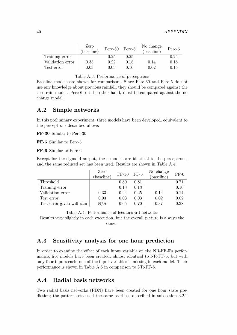
Training error 0.25 0.25 0.24Validation error 0.33 0.22 0.18 0.14 0.18Test error 0.03 0.03 0.16 0.02 0.15

Table A.3: Performance of perceptronsBaseline models are shown for comparison. Since Perc-30 and Perc-5 do notuse any knowledge about previous rainfall, they should be compared against thezero rain model. Perc-6, on the other hand, must be compared against the nochange model.

A.2 Simple networks

In this preliminary experiment, three models have been developed, equivalent tothe perceptrons described above:

FF-30 Similar to Perc-30



Except for the sigmoid output, these models are identical to the perceptrons,and the same reduced set has been used. Results are shown in Table A.4.

Zero(baseline) FF-30 FF-5

No change(baseline) FF-6

Threshold 0.80 0.81 0.71Training error 0.13 0.13 0.10Validation error 0.33 0.24 0.25 0.14 0.14Test error 0.03 0.03 0.03 0.02 0.02Test error given will rain N/A 0.65 0.70 0.37 0.38

Table A.4: Performance of feedforward networksResults vary slightly in each execution, but the overall picture is always the

same.

A.3 Sensitivity analysis for one hour prediction

In order to examine the effect of each input variable on the NR-FF-5’s perfor-mance, five models have been created, almost identical to NR-FF-5, but withonly four inputs each; one of the input variables is missing in each model. Theirperformance is shown in Table A.5 in comparison to NR-FF-5.

A.4 Radial basis networks

Two radial basis networks (RBN) have been created for one hour state pre-diction; the pattern sets used the same as those described in subsection 3.2.2

A.5. ONE-HOUR VALUE PREDICTION 41

Variable missingNR-FF-5 Wind x Wind y Tem Hum Pres

Threshold 0.85 0.85 0.83 0.84 0.82 0.73Training error 0.15 0.15 0.16 0.16 0.17 0.17Validation error (VE) 0.32 0.32 0.32 0.32 0.33 0.32VE given will rain 0.94 0.94 0.92 0.93 0.95 0.95VE giv. won’t rain 0.016 0.016 0.021 0.021 0.021 0.005Test error (TE) 0.016 0.016 0.015 0.016 0.019 0.014TE given will rain 0.94 0.94 0.93 0.93 0.95 0.96TE giv. won’t rain 0.007 0.007 0.006 0.007 0.010 0.004No rain giv. pred. rain 0.92 0.92 0.89 0.90 0.95 0.90

Table A.5: Performance of sensitivity analysis models for one hour prediction

(page 28).

• RBN-5 has been created with a target mean square error of 250, resultingin 5 nodes in the hidden layer.

• RBN-87 has been created with a target mean square error of 200, resultingin 87 nodes in the hidden layer.

Performance is shown in Table A.6.

5-3-3 RBN 87 RBN 5Threshold 0.85 0.77 0.69Training error 200 250Validation error (VE) 0.31 0.32 0.32VE given will rain 0.90 0.89 0.88VE giv. won’t rain 0.016 0.016 0.024Test error (TE) 0.011 0.037 0.035TE given will rain 0.93 0.89 0.90TE giv. won’t rain 0.002 0.014 0.012No rain giv. pred. rain 0.72 0.83 0.81

Table A.6: Performance of radial basis networks

A.5 One-hour value prediction

It is not clear whether we should create two different models, one for the case ofraining now, and one for the case of not raining now. Thus, we both ways areattempted. The names of the models are preceeded by R or NR as previously,or by S for the case of a single network. The R case is not be considered.

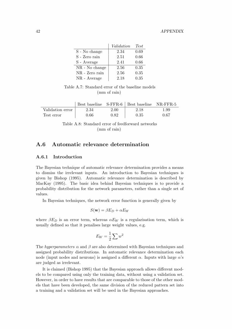
The no change, zero rain, and average baseline models can be used. Theirperformance is shown in Table A.7.

Two models have been developed, the S-FFR-6 and NR-FFR-5, which are al-most identical to FF-6 and NR-FF-5, the only difference being that their outputis not passed through a hard limiting function. Results are shown in Table A.8.

42 APPENDIX

Validation TestS - No change 2.34 0.69S - Zero rain 2.51 0.66S - Average 2.41 0.66NR - No change 2.56 0.35NR - Zero rain 2.56 0.35NR - Average 2.18 0.35

Table A.7: Standard error of the baseline models(mm of rain)

Best baseline S-FFR-6 Best baseline NR-FFR-5Validation error 2.34 2.00 2.18 1.99Test error 0.66 0.82 0.35 0.67

Table A.8: Standard error of feedforward networks(mm of rain)

A.6 Automatic relevance determination

A.6.1 Introduction

The Bayesian technique of automatic relevance determination provides a meansto dismiss the irrelevant inputs. An introduction to Bayesian techniques isgiven by Bishop (1995). Automatic relevance determination is described byMacKay (1995). The basic idea behind Bayesian techniques is to provide aprobability distribution for the network parameters, rather than a single set ofvalues.

In Bayesian techniques, the network error function is generally given by

S(w) = βED + αEW

where βED is an error term, whereas αEW is a regularisation term, which isusually defined so that it penalises large weight values, e.g.

EW =12

∑w2

The hyperparameters α and β are also determined with Bayesian techniques andassigned probability distributions. In automatic relevance determination eachnode (input nodes and neurons) is assigned a different α. Inputs with large α’sare judged as irrelevant.

It is claimed (Bishop 1995) that the Bayesian approach allows different mod-els to be compared using only the training data, without using a validation set.However, in order to have results that are comparable to those of the other mod-els that have been developed, the same division of the reduced pattern set intoa training and a validation set will be used in the Bayesian approaches.

A.6. AUTOMATIC RELEVANCE DETERMINATION 43

A.6.2 Models and results

The following models have been created for automatic relevance determination,all with one hidden layer:

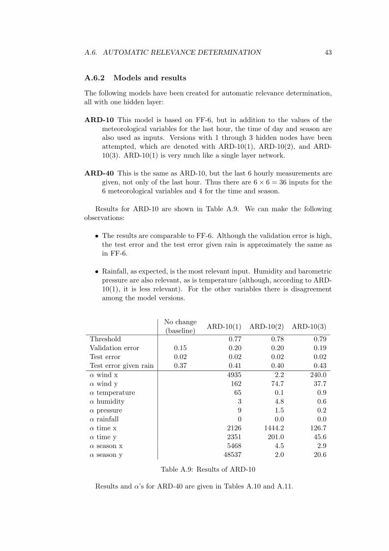
ARD-10 This model is based on FF-6, but in addition to the values of themeteorological variables for the last hour, the time of day and season arealso used as inputs. Versions with 1 through 3 hidden nodes have beenattempted, which are denoted with ARD-10(1), ARD-10(2), and ARD-10(3). ARD-10(1) is very much like a single layer network.

ARD-40 This is the same as ARD-10, but the last 6 hourly measurements aregiven, not only of the last hour. Thus there are 6× 6 = 36 inputs for the6 meteorological variables and 4 for the time and season.

Results for ARD-10 are shown in Table A.9. We can make the followingobservations:

• The results are comparable to FF-6. Although the validation error is high,the test error and the test error given rain is approximately the same asin FF-6.

• Rainfall, as expected, is the most relevant input. Humidity and barometricpressure are also relevant, as is temperature (although, according to ARD-10(1), it is less relevant). For the other variables there is disagreementamong the model versions.

No change(baseline) ARD-10(1) ARD-10(2) ARD-10(3)

Threshold 0.77 0.78 0.79Validation error 0.15 0.20 0.20 0.19Test error 0.02 0.02 0.02 0.02Test error given rain 0.37 0.41 0.40 0.43α wind x 4935 2.2 240.0α wind y 162 74.7 37.7α temperature 65 0.1 0.9α humidity 3 4.8 0.6α pressure 9 1.5 0.2α rainfall 0 0.0 0.0α time x 2126 1444.2 126.7α time y 2351 201.0 45.6α season x 5468 4.5 2.9α season y 48537 2.0 20.6

Table A.9: Results of ARD-10

Results and α’s for ARD-40 are given in Tables A.10 and A.11.

44 APPENDIX

No change(baseline) ARD-40

Threshold 0.88Validation error 0.15 0.20Test error 0.02 0.03Test error given rain 0.37 0.41

Table A.10: Results of ARD-40

Hours ago Wind x Wind y Temp. Hum. Pres. Rain0 2.1 2.1 0.3 0.2 0.5 0.01 11.1 3.5 0.9 0.5 0.5 0.12 1.5 1.9 4.2 1.1 0.5 0.23 77.6 7.1 1.9 39.7 6.3 1.24 6.2 4.5 0.6 1.6 5.2 0.55 1.7 107.8 1.2 1.2 1.0 0.3

Time vector Month vector170.8 1750.6 4.3 5.9

Table A.11: α for the various inputs for ARD-40

A.6.3 Discussion

It can be seen that there are some problems in this method. First, we observethat one version of a model produces completely different results from another,similar model. There does exist an explanation for this: input variable A alonemight be irrelevant, input variable B alone might be irrelevant, but some nonlin-ear function f(A,B) might be relevant. For a model to correctly determine therelevance of A and B in that case, both variables must be given as inputs, andthe model must be complex enough to determine the nonlinear function f . It isthus expected that the results of ARD-10(3), which has more hidden layers andcan create more complex relations, are better than those of the other models.However, this explanation can hardly account for all the differences in the threeversions of ARD-10.

Perhaps the most important problem of ARD is that it does not accountfor correlations of the input variables. If in an ARD model two of the inputvariables are identical, then the model would find them to be equally relevant,and it might be that they would both be very relevant; however, we could safelyget rid of one of them. Similarly, humidity is correlated with rainfall; whenit rains, humidity frequently approaches 100%. As a result, although ARD-10finds humidity to be very relevant, it offers little additional information. It maythus better to use other methods in place of ARD, such as sensitivity analysisor principal component analysis.

Bibliography

Atiya, A. F., S. M. El-Shoura, S. I. Shaheen, and M. S. El-Sherif, “A com-parison between neural-network forecasting techniques—case study: Riverflow forecasting”, IEEE Transactions on Neural Networks 10 (2), 402–409,1999.

Atkinson, B. W., and A. Gadd, Weather: A Modern Guide to Forecasting,Mitchell Beazley Publishers, 1986.

Bishop, C. M., Neural Networks for Pattern Recognition, Clarendon Press,1995.

Fox, B., “Advantage, BBC, thanks to the rain radar”, New Scien-tist 163 (2193), 6, 1999.

Khotanzad, A., M. H. Davis, A. Abaye, and D. J. Maratukulam, “An artificialneural network hourly temperature forecaster with applications in loadforecasting”, IEEE Transactions on Power Systems 11 (2), 870–876, 1996.

Kuligowski, R. J., and A. P. Barros, “Experiments in short-term precipita-tion forecasting using artificial neural networks”, Monthly Weather Re-view 126 (2), 470–482, 1998.

Lapedes, A., and R. Farber, “How neural nets work”, in Y. C. Lee (Ed.),Evolution, Learning and Cognition, World Scientific, 1988. Also in Neu-ral Information Processing Systems, edited by D. Z. Anderson, AmericanInstitute of Physics, 1988.

MacKay, D. J. C., “Bayesian methods for backpropagation networks”, inE. Domany, J. L. van Hemmen, and K. Schulten (Eds.), Models of NeuralNetworks III: Association, Generalization, and Representation, Springer,1995.

Mamassis, N., D. Koutsoyiannis, and A. Christofides, “Experience from theoperation of the automatic telemetric meteorological station of the Na-tional Technical University of Athens”, in Proceedings of the 8th NationalCongress of the Hellenic Hydrotechnical Union, 2000. In Greek.

Murphy, A. H., “Forecast verification”, in R. W. Katz and A. H. Murphy(Eds.), Economic Value of Weather and Climate Forecasts, CambridgeUniversity Press, 1997.

Richardson, L. F., Weather Prediction by Numerical Process, Cambridge Uni-versity Press, 1922.

45

46 BIBLIOGRAPHY

See, L., and S. Openshaw, “Applying soft computing approaches to river levelforecasting”, Hydrological Sciences Journal 44 (5), 763–778, 1999.

Tribbia, J. J., “Weather prediction”, in R. W. Katz and A. H. Murphy (Eds.),Economic Value of Weather and Climate Forecasts, Cambridge UniversityPress, 1997.

SHORT-TERM RAIN PREDICTION WITH ARTIFICIAL NEURAL NETWORKS · SHORT-TERM RAIN PREDICTION WITH...

Documents

Transcript of SHORT-TERM RAIN PREDICTION WITH ARTIFICIAL NEURAL NETWORKS · SHORT-TERM RAIN PREDICTION WITH...