Short Introduction to LS-DYNA and LS-PrePost - Division of Solid
74
Short Introduction to LS-DYNA and LS-PrePost Jimmy Forsberg
Transcript of Short Introduction to LS-DYNA and LS-PrePost - Division of Solid

Short Introduction to LS-DYNA and LS-PrePost
Jimmy Forsberg
Content
■ DYNAmore Nordic presentation
■ Introduction to LS-DYNA
■ General work with different solvers.
■ LS-DYNA capabilities
■ Keywordfile structure
■ Introduction to LS-PrePost
■ Layout
■ Pre-processing
■ Post-processing
■ Special features
■ Composite tool
2013-09-09 4 Test

DYNAmore Group
■ CAE Software
■ Engineering services
■ Distributor for LSTC
■ Personnel: 70
■ LSTC code developer: 10
■ Head office in
Stuttgart, Germany
5

DYNAmore Group
■ Sweden ■ 17 Employees
■ 37 years in average
■ 9 Ph.D.
■ 8 M.Sc.
■ 1 Economics/Adm
■ Office in Linköping
■ Office in Göteborg
6

DYNAmore GmbH
7
Germany
■ ~60 Employees
■ Headquarters in Stuttgart-Vaihingen
■ Offices
■ Ingolstadt
■ Dresden
■ Wolfsburg
■ Fürstenwalde (Berlin)
■ On-site Offices
■ Sindelfingen
■ Untertürkheim
■ Weissach
■ Ingolstadt
Stuttgart [Headquarters]
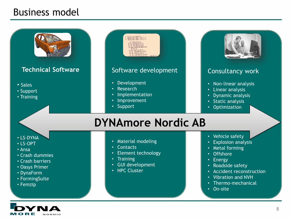
Business model
8
Technical Software
• Sales
• Support
• Training
• LS-DYNA
• LS-OPT
• Ansa
• Crash dummies
• Crash barriers
• Oasys Primer
• DynaForm
• FormingSuite
• Femzip
Software development
• Development
• Research
• Implementation
• Improvement
• Support
• Material modeling
• Contacts
• Element technology
• Training
• GUI development
• HPC Cluster
Consultancy work
• Non-linear analysis
• Linear analysis
• Dynamic analysis
• Static analysis
• Optimization
• Vehicle safety
• Explosion analysis
• Metal forming
• Offshore
• Energy
• Roadside safety
• Accident reconstruction
• Vibration and NVH
• Thermo-mechanical
• On-site
DYNAmore Nordic AB

DYNAmore Group – Selected customers
10

Contact
11
■ Software Products
■ Dr. Marcus Redhe
■ E-mail: [email protected]
■ Mobile: +46 – (0)70 55 131 42
■ Engineering Service and Support
■ Dr. Daniel Hilding
■ E-mail: [email protected]
■ Mobile: +46 – (0)70 65 366 85
■ Address:
DYNAmore Nordic
Brigadgatan 14
587 58 Linköping
Sweden
■ Web: http://www.dynamore.se
■ Phone: +46 – (0)13 23 66 80

Introduction to LS-DYNA
2013-09-09 Test 12

One code strategy
“Combine the multi-physics capabilities into one scalable code for solving
highly nonlinear transient problems to enable the solution of coupled multi-
physics and multi-stage problems”
LS-DYNA
Explicit/Implicit
Heat Transfer
Mesh Free EFG,SPH,Airbag Particle
User Interface Elements, Materials, Loads
Acoustics Frequency
Response, Modal Methods
Discrete Element Method
Incompressible Fluids
CESE Compressible Fluid
Solver
Electromagnetism
R7
R7
R7

SBD – Simulation Based Design
■ Instead of a physical prototype, a virtual model is created. The purpose of the model is to resemble the behaviour of the physical product.
■ All development/testing is made in the virtual product. Thus, you treat the model as you would if it was a physical product.
■ The benefits are several: ■ Shorter time to market
■ Reduce number of costly prototypes
■ Increased innovation
■ Lower development costs
■ Higher quality
■ … but also the challenges ■ Rethink development process
■ Trust the results
■ Educate personnel, new partners..

Volvo XC60
15

What do you need?
PRE-PROCESSOR
Generates the FE-model
Applies boundary conditions etc
SOLVER
Solves the numerical model
POST-PROCESSOR
View the results
History?
Geometry
Material
Process
LS-DYNA
Dependence on analysis LS-PrePost
17
LS-PrePost

Modify
-Process
- Initial powder volume
-Geometry
Simulation process
2013-09-09 Test 18
Build FE-model
-Parts
-Material
-Element
LS-DYNA
LS-PrePost/ANSA
Pre – simulation?
-Initial stress/stress?
- Bolts etc.
LS-PrePost
LS-DYNA
Evaluate results
LS-PrePost
LS-PrePost

Introduction to LS-DYNA
2013-09-09 Test 19

Keywords and Elements

Keywords - Define Geometry
2013-09-09 Keyword and Elements 21
Input file (.k)
length meter millimeter millimeter
time second second millisecond
mass kilogram tonne kilogram
force Newton Newton kiloNewton
Young’s modulus of steel 210.0E+09 210.0E+03 210.0
density of steel 7.85E+03 7.85E-09 7.85E-06
gravitation 9.81 9.81E+03 9.81E-03
Newton’s second law, F=ma, requires consistent units
S1 S2 S3

Keyword User’s manual
2013-09-09 Keyword and Elements 22

Input file - Keywords
2013-09-09 Keyword and Elements 23
*KEYWORD
*TITLE
Test example
$ Control cards govern entire model / simulation
*CONTROL_TERMINATION
*CONTROL_TIMESTEP
$ Define output of results
*DATABASE_BINARY_D3PLOT
*DATABASE_GLSTAT
$ Define section and material
*PART
$ Define element types and integration
*SECTION_SHELL
$ Define material properties
*MAT_ELASTIC
*MAT_FIBER
$ Define nodes and elements
*NODE
*ELEMENT_SHELL
$ Define loads and BC
*LOAD_NODE
*END
Mandatory
Mandatory
Input file (.k)
Comment card
begins with $
PART
Material Section
Element

Keyword Format
2013-09-09 Keyword and Elements 24
Input file (.k) ■ Similar functions are grouped together under
the same keyword
■ A data block begins with a keyword and ends
with the next keyword
■ Keywords are left justified
■ No distinction between lower and upper case
letters
■ Variables are right justified in their fields
■ A ‘0’ or blank means that the variable will get
the default value
■ The decimal point is always written out for
floating point variables

Keyword Format
2013-09-09 Keyword and Elements 25
Input file (.k) ■ Comments rows are written after a dollar sign in
the first position
■ *COMMENT keyword exist
■ Do not use ‘tabs’ when editing or creating your
file
■ Line feed signs may cause problems when
transferring files from Dos to Unix

Keywords - Define Geometry
26
Input file (.k) PART
Material Section
Element
*NODE
$ NID * x * y * z *
1 0.00 0.00 0.00
2 1.0E-2 0 0
3 0.02 0 0
4 2.0E-2 1.0E-2 0
5, 0.01, 0.01, 0.0
6, 0.02, 0.01, 0
$
$
*ELEMENT_SHELL
$ID, PID, n1, n2, n3, n4
1, 1, 1, 2, 5, 4
2, 1, 2, 3, 6, 5
0 0.01 0.02
0.01
0
e1 e2
0.02
x
y
n1 n2 n3
n4 n5 n6
Free format Fix
ed f
orm
at
e1
1 2
5 4
ye1
xe1
Xe1: from n1 to n2
Local coordinate system:
ye1: perpendicular to xe1
directed towards n3
2013-09-09 Keyword and Elements

Elements
■ Some element formulations are more
costly than others
■ Stresses and strains are calculated at the
integration points
■ Accelerations, velocities and
displacements are evaluated at the nodes
2013-09-09 Keyword and Elements 27

Under Integrated and Fully Integrated Elements
■ Most element formulations in LS-DYNA are under-
integrated, i.e. the stresses and strains are only
calculated in the mid-point of each element.
■ Advantage: Computational efficiency. The material model
is called once per integration point and time step.
■ Disadvantage: The element formulation contains zero-
energy modes (hourglass modes)
2013-09-09 Keyword and Elements 28
Integration
point (s)

Under Integrated and Fully Integrated Elements
■ The following element deformation does not yield any
strains in the integration point, and thus no stress
■ There is deformation, but no associated internal energy,
hence the name zero-energy modes.
■ These modes have to be suppressed using ”hourglass
control”
2013-09-09 Keyword and Elements 29
“No strain” x
x

Hourglass Control
■ Zero energy modes = Hourglass modes
■ Hourglass controlled by *CONTROL_HOURGLASS and
*HOURGLASS
■ Hourglass modes for 1 point integration Q4 shell
elements:
■ Hourglass modes for 1 point integration solid elements:
2013-09-09 Keyword and Elements 30
+ 8 more!
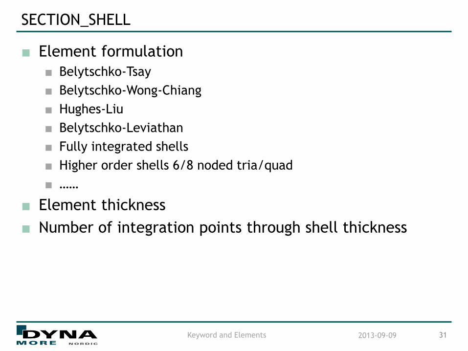
SECTION_SHELL
■ Element formulation
■ Belytschko-Tsay
■ Belytschko-Wong-Chiang
■ Hughes-Liu
■ Belytschko-Leviathan
■ Fully integrated shells
■ Higher order shells 6/8 noded tria/quad
■ ……
■ Element thickness
■ Number of integration points through shell thickness
2013-09-09 Keyword and Elements 31

Elements (shell) - NIP
■ 1 point integration through the thickness gives a
membrane element
■ 2 point integration through the thickness is the default
(sufficient for a linearly elastic material)
■ For plastic bending behaviour, at least 3 points are
needed through the thickness
■ 5 points recommended for sheet metal stamping.
7 points for springback
■ Use odd numbers to include the neutral axis
2013-09-09 Keyword and Elements 32
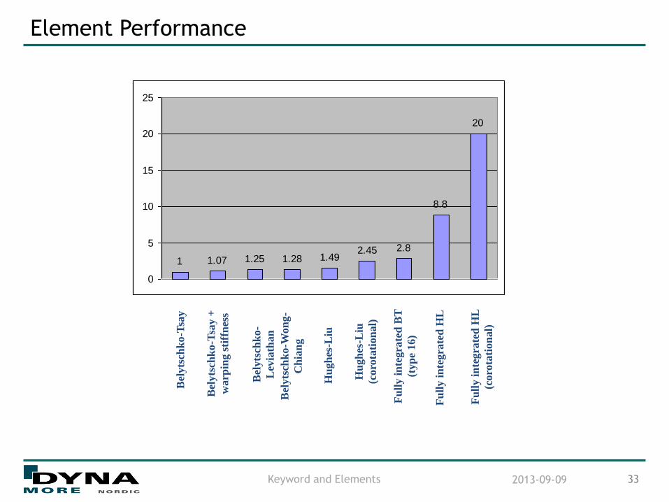
Element Performance
2013-09-09 Keyword and Elements 33
Bel
yts
chk
o-T
say
Bel
yts
chk
o-T
say +
warp
ing s
tiff
nes
s
Bel
yts
chk
o-
Lev
iath
an
1 1.07 1.25 1.28 1.49
2.45 2.8
8.8
20
0
5
10
15
20
25
Bel
yts
chk
o-W
on
g-
Ch
ian
g
Hu
gh
es-L
iu
Fu
lly i
nte
gra
ted
BT
(typ
e 16)
Hu
gh
es-L
iu
(coro
tati
on
al)
Fu
lly i
nte
gra
ted
HL
Fu
lly i
nte
gra
ted
HL
(coro
tati
on
al)

*CONTROL_ACCURACY
■ Invariant node numbering
■ particularly important when large shear forces are present in an
element
■ 2nd order stress update
■ spinning bodies such as turbine blades, rotating tires
■ sometimes for stiffness hourglass control
■ implicit solutions with large strains in each step
2013-09-09 Keyword and Elements 34

Material Models

Material Models
■ Over 200 models for various applications exists in
LS-DYNA.
■ Determine the stress based on strain, strain-rate,
temp etc.
■ Not materials, but models subject to restrictions:
■ Load magnitude
■ Deformation speed (strain rate)
■ Temperature
■ The models are defined by material parameters
■ E, , , etc.
2013-09-09 Material Models 36

Hypoelasticity
Hypoelasticity relates a strain rate to a corresponding stress
rate
Stress is incrementally updated from the strain rate with
aid of the constitutive tensor C
Most of the materials in LS-DYNA are based on this
formulation for the elastic response.
2013-09-09 Material Models 37
D:Cσ
tD
t
E
Hooke’s law:

Merits and drawbacks (theoretical)
+ ■ It is fairly straightforward to use and easy to implement
in a finite element code
-
■ The response is path-dependent, the stress for a closed strain cycle can be nonzero, it should be used when the elastic deformation is relatively small
■ It is difficult to deal with anisotropic constitutive models because the constitutive tensor C is restricted to be isotropic for nonlinear analysis. This is however solved in LS-DYNA with a co-rotational update.
2013-09-09 Material Models 38

Hyperelasticity - definition
■ A material is hyperelastic if the internal work is
independent of the deformation path.
■ It is characterized by the existence of a strain energy
function that is a potential for the stress.
■ Typically used when elastic deformation is substantial,
e.g. rubber.
2013-09-09 Material Models 39
E
E
C
CS
)()(2
W
orGreen tens-CauchyRight
sorstrain tenGreen
tensorstress Kirchhoff Piola Second
C
E
S

Stress and strain – uni-axial deformation
2013-09-09 Material Models 40
Tensile test:
Engineering stress
Engineering strain
In LS-DYNA:
True stress
True strain
Elastic response:
Hooks law:
Area reduction:
0E A/F
00E L/)LL(
A/F
)L/Lln( 0
L
0L
F F
0A A
)21(AA 0
Eεσ
σ
ε
E

Elasto-plasticity in 3-D – multi-axial deformation
2013-09-09 Material Models 41
Stress decomposition……….:
Von Mises yield criterion….:
Plastic strain…………………:
)(23
pyijijssf
3/S kkijijij
Volumetric stress
Deviatoric stress
ij
p
ijS
f
1
32
1
32
1
32
Perfect plasticity Isotropic hardening Kinematic hardening
p
ijεp
ijεp
ijε

Elastic-visco-plastic material
2013-09-09 Material Models 42
*MAT_PIECEWISE_LINEAR_PLASTIC MID RO E PR SIGY ETAN FAIL TDEL
C P LCSS LCSR VP
EPS1 EPS2 . . . . . . . . . .
EP1 ES2 . . . . . . . . . .
For: Metals, loading exceeding yielding stress, rate effects
In: All element types
Theory: Isotropic plasticity model with visco-plasticity option
E Young's Modulus C,P Strain-rate parameters
RO Density LCSS Load curve for
PR Poisson's Ratio LCSR Load curve for strain-rate scaling
SIGY Yield stress VP Visco-plastic flag
ETAN Tangent modulus EPS1… Piecewise linear def.

Elastic-visco-plastic material
2013-09-09 Material Models 43
Activating visco-plasticity: ( =static yield stress )
No visco-plastic effects
Scale by:
Scale by:
Yield stress is given by:
VP=1 is recommended as it uses a consistent
visco-plastic theory
0P,C
1VP,0P,C
1VP,0P,C
0VP,0P,Cijij
P
C
,1
1
kkijijij
P1
e,C
e1
Pp
effs
yyC
1
1
s
y
s
y
s
y

Elastic-plastic material with Bauschinger efftect
2013-09-09 Material Models 44
*MAT_PLASTIC_KINEMATIC MID RO E PR SIGY ETAN BETA
SRC SRP FS VP For: Metals under large loading
In: All element types
Theory: Isotropic and kinematic hardening plasticity, viscoplastic
E Young's Modulus
RO Density
PR Poisson's Ratio
SIGY Yield stress
ETAN Tangent modulus
BETA Hardening parameter FS Failure strain
SRC Strain rate parameter C VP Rate formulation flag
SRP Strain rate parameter P

Elastic-plastic material with Bauschinger efftect
2013-09-09 Material Models 45
Definition of material hardening:
Other models with kinematic hardening:
*MAT_PLASTIC_GREEN-NAGHDI_RATE
*MAT_ANISOTROPIC_VISCOPLASTIC
Kinematic hardening
Isotropic hardening
E
0y
ETAN
0y2
1y2
1y2
1
0

*EOS
■ Certain material models only solve for the deviatoric part
of the stress tensor
■ An Equation of State (EOS) is required to find the
pressure part of the stress tensor
■ Mostly used in conjunction with fluid-like behaviour (high
explosives, airbag inflation …)
■ Solid elements only
2013-09-09 Material Models 46

Boundary/Initial Conditions

Initial and Boundary Conditions
■ Variation in time using load curves
■ Variation in space
■ Arbitrary directions using
■ Local coordinate systems
■ Vectors
But limited to cartesian coordinates
2013-09-09 Initial/Boundary Conditions 48
)t(u
)t(Traction
)t(b

*LOAD
2013-09-09 Initial/Boundary Conditions 49
*LOAD_NODE[_SET|_POINT]
NODE/NSID DOF LCID SF CID M1 M2 M3
Nodal loads for one node or a set of nodes
DOF Direction of load in current coordinate system LCID Load curve ID for variation in time SF Scale load curve amplitude CID Define a local coordinate system M1-M3 Follower force definition
Singularities at point loads may be a problem.
Multiple load cards are accumulated.
F
F
1M
3M
2M

*INITIAL
2013-09-09 Initial/Boundary Conditions 50
*INITIAL_STRESS[_BEAM|_SHELL|_SOLID] *INITIAL_STRAIN[_SHELL|_SOLID]
Initialise the state of stress and strain in elements
Normally used to carry results obtained in one simulation to another. - Multistage forming
- Forming -> Crash Keyword data normally generated automatically by preprocessors.

Kinematic Conditions
■ Prescribe motion in the model
■ *BOUNDARY: w.r.t cartesian coordinates
■ Fixed supports
■ Symmetric boundaries
■ *CONSTRAINED: internal definitions
■ Mechanical Joints
■ Merging shell-brick elements
■ Define rigid bodies
2013-09-09 Initial/Boundary Conditions 51
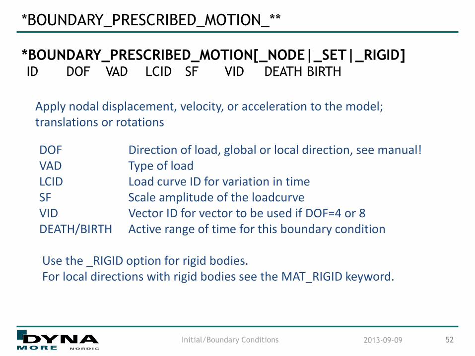
*BOUNDARY_PRESCRIBED_MOTION_**
2013-09-09 Initial/Boundary Conditions 52
*BOUNDARY_PRESCRIBED_MOTION[_NODE|_SET|_RIGID] ID DOF VAD LCID SF VID DEATH BIRTH
Apply nodal displacement, velocity, or acceleration to the model; translations or rotations
DOF Direction of load, global or local direction, see manual! VAD Type of load LCID Load curve ID for variation in time SF Scale amplitude of the loadcurve VID Vector ID for vector to be used if DOF=4 or 8 DEATH/BIRTH Active range of time for this boundary condition Use the _RIGID option for rigid bodies. For local directions with rigid bodies see the MAT_RIGID keyword.

*CONSTRAINED
2013-09-09 Initial/Boundary Conditions 53
*CONSTRAINED_NODAL_RIGID_BODY PID CID NSID PNODE IPRT
Create a new rigid body using existing nodes PID Part id req. is a unique one CID Coordinate system for output NSID Node set PNODE Optional centre node IPRT Print flag
For spot-welds and other types of rigid connections.
RB
*CONSTRAINED
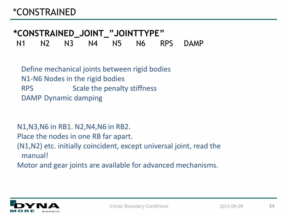
2013-09-09 Initial/Boundary Conditions 54
*CONSTRAINED_JOINT_”JOINTTYPE” N1 N2 N3 N4 N5 N6 RPS DAMP
Define mechanical joints between rigid bodies N1-N6 Nodes in the rigid bodies RPS Scale the penalty stiffness DAMP Dynamic damping
N1,N3,N6 in RB1. N2,N4,N6 in RB2. Place the nodes in one RB far apart. (N1,N2) etc. initially coincident, except universal joint, read the manual! Motor and gear joints are available for advanced mechanisms.
*CONSTRAINED
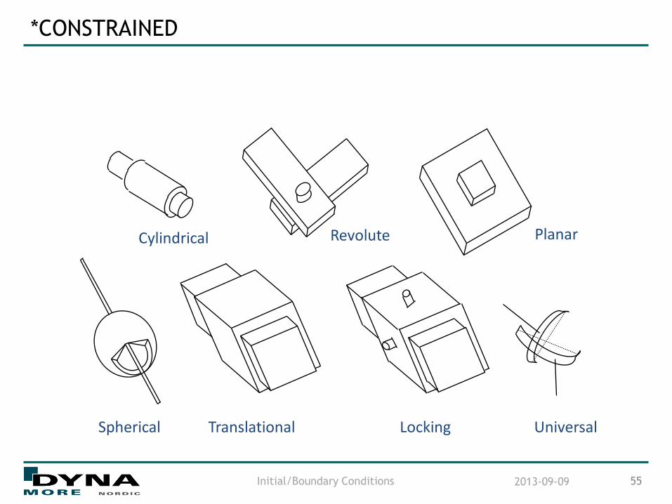
2013-09-09 Initial/Boundary Conditions 55
Cylindrical Revolute Planar
Spherical Translational Universal Locking

Contacts
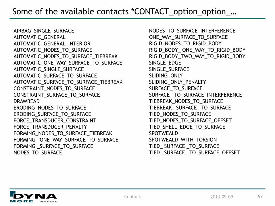
Some of the available contacts *CONTACT_option_option_…
2013-09-09 Contacts 57
AIRBAG_SINGLE_SURFACE
AUTOMATIC_GENERAL
AUTOMATIC_GENERAL_INTERIOR
AUTOMATIC_NODES_TO_SURFACE
AUTOMATIC_NODES_TO_SURFACE_TIEBREAK
AUTOMATIC_ONE_WAY_SURFACE_TO_SURFACE
AUTOMATIC_SINGLE_SURFACE
AUTOMATIC_SURFACE_TO_SURFACE
AUTOMATIC_SURFACE_TO_SURFACE_TIEBREAK
CONSTRAINT_NODES_TO_SURFACE
CONSTRAINT_SURFACE_TO_SURFACE
DRAWBEAD
ERODING_NODES_TO_SURFACE
ERODING_SURFACE_TO_SURFACE
FORCE_TRANSDUCER_CONSTRAINT
FORCE_TRANSDUCER_PENALTY
FORMING_NODES_TO_SURFACE_TIEBREAK
FORMING _ONE_WAY_SURFACE_TO_SURFACE
FORMING _SURFACE_TO_SURFACE
NODES_TO_SURFACE
NODES_TO_SURFACE_INTERFERENCE
ONE_WAY_SURFACE_TO_SURFACE
RIGID_NODES_TO_RIGID_BODY
RIGID_BODY_ ONE_WAY_TO_RIGID_BODY
RIGID_BODY_TWO_WAY_TO_RIGID_BODY
SINGLE_EDGE
SINGLE_SURFACE
SLIDING_ONLY
SLIDING_ONLY_PENALTY
SURFACE_TO_SURFACE
SURFACE _TO_SURFACE_INTERFERENCE
TIEBREAK_NODES_TO_SURFACE
TIEBREAK_ SURFACE _TO_SURFACE
TIED_NODES_TO_SURFACE
TIED_NODES_TO_SURFACE_OFFSET
TIED_SHELL_EDGE_TO_SURFACE
SPOTWEALD
SPOTWEALD_WITH_TORSION
TIED_ SURFACE _TO_SURFACE
TIED_ SURFACE _TO_SURFACE_OFFSET

Contact
■ A way of treating interaction between different parts
■ Contacts are defined by sets (node/part/segments) or a box
■ Generally there is a master side and a slave side of the contact
■ The master side can be a mathematically described with a geometrical surface (rigid)
■ The thickness of shells are normally taken into account
■ Most recommended contacts are based on the penalty method
■ Several contacts treating special applications exists
■ Old contact types kept for compatibility reasons
2013-09-09 Contacts 58
Motion
MASTER
SLAVE
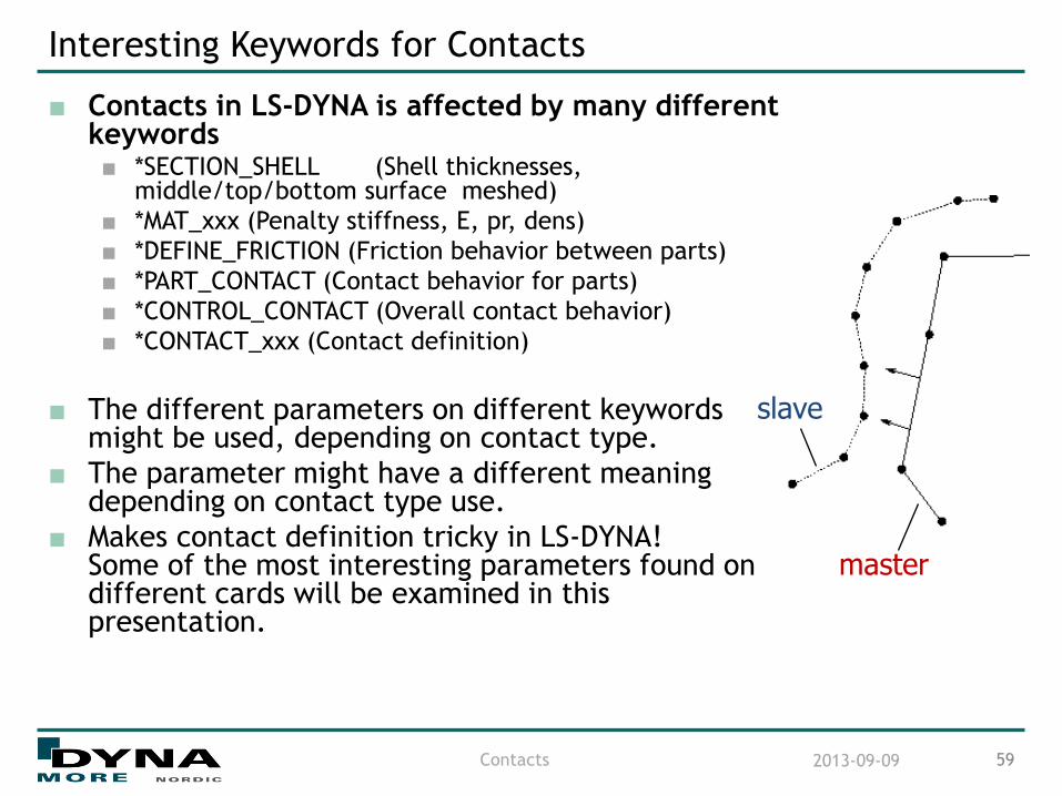
Interesting Keywords for Contacts
■ Contacts in LS-DYNA is affected by many different keywords ■ *SECTION_SHELL (Shell thicknesses,
middle/top/bottom surface meshed)
■ *MAT_xxx (Penalty stiffness, E, pr, dens)
■ *DEFINE_FRICTION (Friction behavior between parts)
■ *PART_CONTACT (Contact behavior for parts)
■ *CONTROL_CONTACT (Overall contact behavior)
■ *CONTACT_xxx (Contact definition)
■ The different parameters on different keywords might be used, depending on contact type.
■ The parameter might have a different meaning depending on contact type use.
■ Makes contact definition tricky in LS-DYNA! Some of the most interesting parameters found on different cards will be examined in this presentation.
2013-09-09 Contacts 59
master
slave

Important contact parameters: penalty method (default)
2013-09-09 Contacts 60
Contact force
Fi= δi k
k= interface spring stiffness
Solid elements Shell elements
K= bulk modulus
c = penalty factor
δi=
penetration
Motion
AV
cKAk
diagonal
cKAk
The time step of the analysis is determined by LS-DYNA from the elements of the FE-mesh without considering the contact interfaces!

Contact Thickness and Initial Penetrations
2013-09-09 Contacts 61
d2
d1
Initial penetration
d2‘
d1‘
Change of shell thickness only for contact treatment

Important contact parameters: friction
■ Sliding friction – FS, FD, DC and VC ■ Defined in keyword *CONTACT
■ Based on Coulomb friction
■ Default values gives no friction
■ FS and FD are static respectively dynamic friction coefficient
■ DC - decay coefficient
■ If FD and FS not are equal, then FD should be less than FS and DC nonzero
■ VC is the coefficient for viscous friction and limits the friction force (typically 3-½ of yield stress)
■ Viscous damping VDC improves stability. For metal contacts use 20% and for soft material 40-60%
2013-09-09 Contacts 62
relVDC
c eFDFSFD
)(

Automatic contacts without self contact
■ *CONTACT_AUTOMATIC_NODES_TO_SURFACE ■ *CONTACT_AUTOMATIC_SURFACE_TO_SURFACE
■ Thickness taken into account
■ Contact surface is offset by half thickness from mid-plane
■ Orientation of segments not needed
■ Contact from both sides
■ Handles disjoint meshes
■ Applies a smooth surface based on a radii at the edges (including free edges)
■ Initial penetrations are detected
■ Possible to change or scale contact thickness
■ Friction and damping available
2013-09-09 Contacts 63

Single-surface contacts (self contact)
■ *CONTACT_AUTOMATIC_SINGLE_SURFACE ■ *CONTACT_AUTOMATIC_GENERAL
■ Same features as the
automatic contacts
■ Only require definition of the slave surface
■ Include self contact
■ Sensitive to initial penetrations
■ Possible to use only one contact definition forthe complete model
■ Beam and edge to edge contacts are included *CONTACT_AUTOMATIC_GENERAL
2013-09-09 Contacts 64

Edge/Beam Contacts
■ *CONTACT_AUTOMATIC_GENERAL (26) ■ exclude interior edges
■ entire length of each exterior edge is checked for contact
■ OBS, the edge cylinder is not affected by OPTT or TH when
using part_contact.
■ *CONTACT_AUTOMATIC_GENERAL_INTERIOR (i26) ■ like *CONTACT_AUTOMATIC_GENERAL,
■ but interior edges are treated like exterior edges
■ Alternative way to treat edge contact:
■ creating null beam elements (*ELEMENT_BEAM,*MAT_NULL)
approximately 1mm in diameter along every edge wished to be
considered for edge-to-edge contact and including these null
beams in a separate AUTOMATIC_GENERAL contact
■ *CONTACT_SINGLE_EDGE (22) ■ Treats only edge-to-edge contact
■ no thickness offset at the contact edge
■ *CONTACT_xxx_MORTAR () ■ edge-to-edge contact
■ no thickness offset at the contact edge
2013-09-09 Contacts 65
d
d/2

Tied contacts
■ CONTACT_TIED_NODES_TO_SURFACE
■ *CONTACT_TIED_SURFACE_TO_SURFACE
■ *CONTACT_TIED_SHELL_EDGE_TO_SURFACE …._OFFSET
■ Possibility to “tie” nodes to a surface (segment)
■ NODES_... and SURFACE_... ties translational d.o.f
■ SHELL_EDGE_.. ties translational and rotational d.o.f
■ Constraint based. Thus, will not work with rigid bodies.
■ …_OFFSET allows for a segment thickness and is penalty based.
■ …_TIEBREAK_... has failure options.
■ Can be used to model glue, spotwelds etc.
2013-09-09 Contacts 66

Control Cards & Execution
Control Cards
■ The purpose is: ■ Activate solution options;
implicit solution, adaptive remeshing, mass scaling …
■ Change default values on options and parameters
■ Remember that: ■ Ordering between them and position are arbitrary
Good practise is to put them first in your input file
■ Do not use more then one control card of each type
■ All control cards are optional except *CONTROL_TERMINATION
2013-09-09 Control Cards & Execution 68

Control Card Default Values
■ Default values exist for all options and most parameters
■ Control cards change default values globally
■ Default values are defined hierarchically
The order between them are:
■ LS-DYNA defaults
■ Control card input
■ Individual Keyword input
■ Set your defaults with the control cards and change the
keyword input where default values not should be used
■ Input of ‘0’ will normally give the default value which is
shown in the manual
2013-09-09 Control Cards & Execution 69

Most Important Control Cards
■ Always consider the following control cards since they can strongly affect your results or output
■ *CONTROL_ACCURACY
■ *CONTROL_CONTACT
■ *CONTROL_ENERGY
■ *CONTROL_HOURGLASS
■ *CONTROL_SHELL
■ *CONTROL_SOLID
■ *CONTROL_TERMINATION
■ *CONTROL_TIMESTEP
2013-09-09 Control Cards & Execution 70

Implicit Solution Types
■ Linear Analysis
● static or dynamic
● single, multi-step
■ Eigenvalue Analysis
● frequencies and mode shapes
● linear buckling loads and modes
● modal analysis: extraction and superposition
● Dynamic analysis by modal superposition (971)
■ Nonlinear Analysis
● Newton, Quasi-Newton, Arclength solution
● static or dynamic
■ default LS-DYNA: static and nonlinear!
2013-09-09 Control Cards & Execution 71

Output Files
■ Binary files (can be viewed in LS-PrePost)
*DATABASE_BINARY_Option
■ ASCII files for more detailed output
(graphs can be shown in LS-PrePost)
*DATABASE_Option
■ Data in the binary and ASCII files is controlled by
*DATABASE_EXTENT_Option
*DATABASE_HISTORY_Option
■ Control files (d3hsp)
■ Message files (messag)
2013-09-09 Control Cards & Execution 72

Output Files
■ D3PLOT (database for complete output states)
■ D3DUMP (complete database for restart)
■ RUNRSF (running restart file, overwritten)
■ D3PART (as D3PLOT but includes just specified parts)
■ D3THDT (database for time history data of element
subsets)
■ D3DRLF (dynamic relaxation database)
■ D3MEAN (CFD database)
■ INTFOR (database for output of contact interface data)
■ XTFILE (extra time history data)
■ D3EIGV (modal data from eigenvalue analysis)
■ D3CRCK (crack data from Winfrith concrete model)
2013-09-09 Control Cards & Execution 73

ASCII Output Files
2013-09-09 Control Cards & Execution 74
■ GLSTAT (global data)
■ MATSUM (material energies)
■ RCFORC (resultant interface forces)
■ SLEOUT (sliding interface energy)
■ NODOUT (nodal point data)
■ ELOUT (element data)
■ SECFORC (cross section forces)
■ RWFORC (rigid wall forces)
■ SSSTAT (subsystem data)
■ DEFORC (discrete elements)
■ NCFORC (nodal interface forces)
■ DEFGEO (deformed geometry)
■ SPCFORC (SPC reaction forces)
■ NODFOR (nodal force groups)
■ ABSTAT (airbag statistics)
■ BNDOUT (boundary condition force/ energy)
■ RBDOUT (rigid body data)
■ GCEOUT (geometric contact entities)
■ JNTFORC (joint force)
■ SBTOUT (seat belt output)
■ AVSFLT (AVS database)
■ SWFORC (nodal constraint reaction forces)
■ MOVIE
■ MPGS
■ TRHIST (trace particle history)
■ TPRINT (thermal output)
■ SPHOUT (SPH data)

2013-09-09 Test 75

Demonstrate LS-PrePost
■ PreProcessing
■ PostProcessing
2013-09-09 Test 76
Thank you!
2013-09-09 77 Test