Shopping cost and brand exploration in online groceryare.berkeley.edu/SGDC/Shopping costs and brand...
53
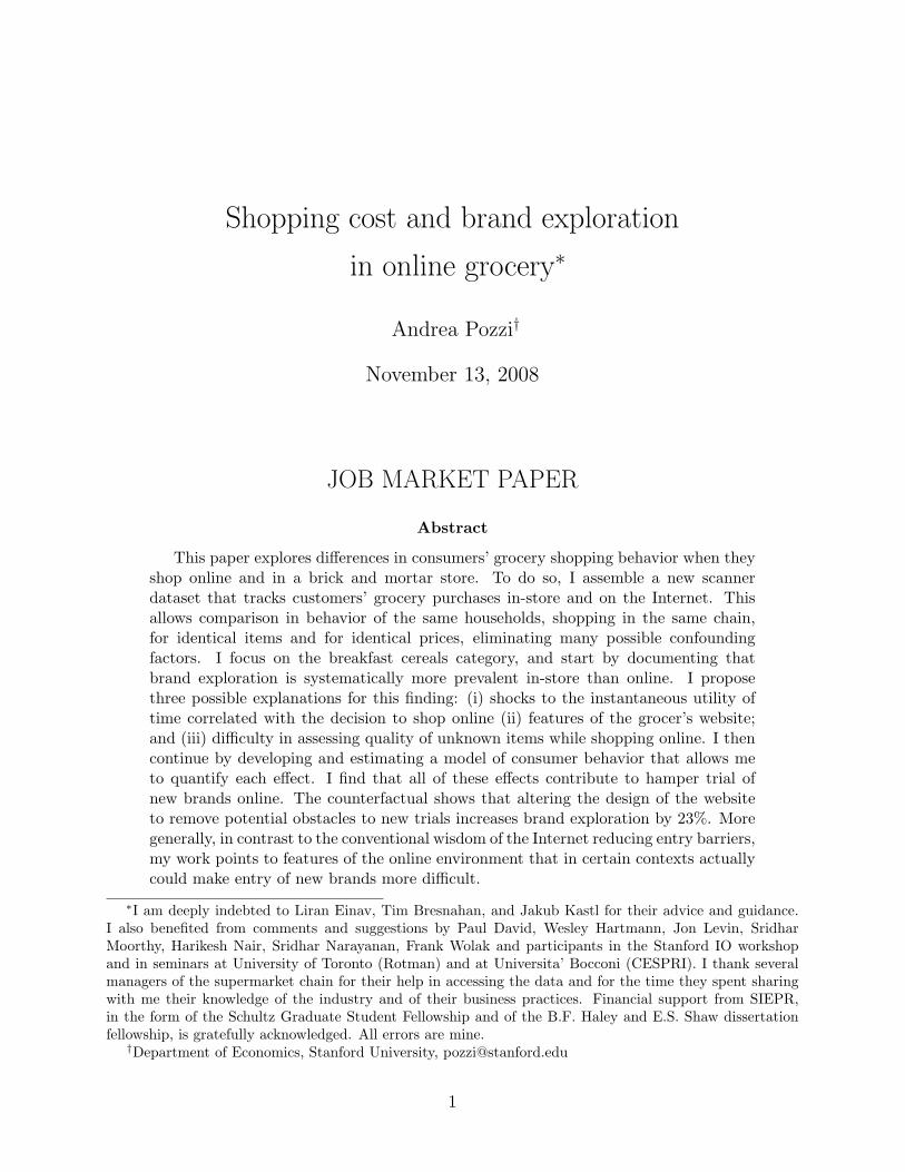
Shopping cost and brand exploration in online grocery * Andrea Pozzi † November 13, 2008 JOB MARKET PAPER Abstract This paper explores differences in consumers’ grocery shopping behavior when they shop online and in a brick and mortar store. To do so, I assemble a new scanner dataset that tracks customers’ grocery purchases in-store and on the Internet. This allows comparison in behavior of the same households, shopping in the same chain, for identical items and for identical prices, eliminating many possible confounding factors. I focus on the breakfast cereals category, and start by documenting that brand exploration is systematically more prevalent in-store than online. I propose three possible explanations for this finding: (i) shocks to the instantaneous utility of time correlated with the decision to shop online (ii) features of the grocer’s website; and (iii) difficulty in assessing quality of unknown items while shopping online. I then continue by developing and estimating a model of consumer behavior that allows me to quantify each effect. I find that all of these effects contribute to hamper trial of new brands online. The counterfactual shows that altering the design of the website to remove potential obstacles to new trials increases brand exploration by 23%. More generally, in contrast to the conventional wisdom of the Internet reducing entry barriers, my work points to features of the online environment that in certain contexts actually could make entry of new brands more difficult. * I am deeply indebted to Liran Einav, Tim Bresnahan, and Jakub Kastl for their advice and guidance. I also benefited from comments and suggestions by Paul David, Wesley Hartmann, Jon Levin, Sridhar Moorthy, Harikesh Nair, Sridhar Narayanan, Frank Wolak and participants in the Stanford IO workshop and in seminars at University of Toronto (Rotman) and at Universita’ Bocconi (CESPRI). I thank several managers of the supermarket chain for their help in accessing the data and for the time they spent sharing with me their knowledge of the industry and of their business practices. Financial support from SIEPR, in the form of the Schultz Graduate Student Fellowship and of the B.F. Haley and E.S. Shaw dissertation fellowship, is gratefully acknowledged. All errors are mine. † Department of Economics, Stanford University, [email protected] 1
Transcript of Shopping cost and brand exploration in online groceryare.berkeley.edu/SGDC/Shopping costs and brand...
Shopping cost and brand exploration
in online grocery∗
Andrea Pozzi†
November 13, 2008
JOB MARKET PAPER
Abstract
This paper explores differences in consumers’ grocery shopping behavior when theyshop online and in a brick and mortar store. To do so, I assemble a new scannerdataset that tracks customers’ grocery purchases in-store and on the Internet. Thisallows comparison in behavior of the same households, shopping in the same chain,for identical items and for identical prices, eliminating many possible confoundingfactors. I focus on the breakfast cereals category, and start by documenting thatbrand exploration is systematically more prevalent in-store than online. I proposethree possible explanations for this finding: (i) shocks to the instantaneous utility oftime correlated with the decision to shop online (ii) features of the grocer’s website;and (iii) difficulty in assessing quality of unknown items while shopping online. I thencontinue by developing and estimating a model of consumer behavior that allows meto quantify each effect. I find that all of these effects contribute to hamper trial ofnew brands online. The counterfactual shows that altering the design of the websiteto remove potential obstacles to new trials increases brand exploration by 23%. Moregenerally, in contrast to the conventional wisdom of the Internet reducing entry barriers,my work points to features of the online environment that in certain contexts actuallycould make entry of new brands more difficult.
∗I am deeply indebted to Liran Einav, Tim Bresnahan, and Jakub Kastl for their advice and guidance.I also benefited from comments and suggestions by Paul David, Wesley Hartmann, Jon Levin, SridharMoorthy, Harikesh Nair, Sridhar Narayanan, Frank Wolak and participants in the Stanford IO workshopand in seminars at University of Toronto (Rotman) and at Universita’ Bocconi (CESPRI). I thank severalmanagers of the supermarket chain for their help in accessing the data and for the time they spent sharingwith me their knowledge of the industry and of their business practices. Financial support from SIEPR,in the form of the Schultz Graduate Student Fellowship and of the B.F. Haley and E.S. Shaw dissertationfellowship, is gratefully acknowledged. All errors are mine.†Department of Economics, Stanford University, [email protected]
1

1 Introduction
Much attention has been devoted in the past decade to understanding the impact of e-
commerce on consumer behavior. In this paper, I study how the choice of the shopping
channel (online or brick and mortar store) affects households’ propensity to try brands they
have not experienced before. I show that households tend to explore less when they shop
for groceries online. My analysis points to features of the Internet -present in this context
but perhaps less likely to exist in the case of more traditional online goods, such as airline
tickets or books- that may make entry barriers higher for new brands.
While representing only 3% of total revenues in retail, online purchases have captured
great shares of the market in several sectors (books, CDs, travel) and are gaining ground in
others (grocery, clothing). Online shopping has not replaced brick and mortar stores, but it
offers an alternative to millions of consumers every year. Given the profound differences in
the shopping experience between online and in-store context, it is natural to ask whether final
demands are also affected. Understanding these differences is therefore crucial for retailers
facing the decision of whether or not to add Internet to the set of their distribution channels,
and how to manage it if they decide to do so. It is also important for manufacturers who may
be interested in possible changes in demand patterns as a result of the increasing relevance
of the online channel.
This study explores a growing online shopping market, that of groceries.1 I assemble
new data containing two years of scanner data for grocery purchases by a panel of some
11,000 consumers who shopped both online and in-store at the same supermarket chain.
In store purchases are tracked through usage of a loyalty card which is also used when
the customer registers for the online service on the grocer’s website. This allows me to
link in-store and online trips for the same household. A number of features of this setting
make it a particularly attractive one for comparison of online and in-store behavior. First,
I observe the same household switching back and forth between the two channels. Most
previous studies compared a sample of online shoppers with a different sample of traditional
shoppers.2 In that case, differences in behavior between the two groups could be in part
due to self selection (i.e., being an online or traditional shopper) rather than caused by
the different medium where the purchase takes place. Moreover, both in-store and online
purchases occur at the same supermarket chain. This ensures that the set of brands carried,
1See Goettler and Clay (2006)2Exceptions are Chu, Chintagunta, and Cebollada (2008) and Brynjolfsson, Hu, and Simester (2006) who
also use a panel of cross channel purchases, but with different focus.
2

prices and promotions, and loyalty to the retail chain are all the same in both channels. If
I were to compare trips at a traditional grocery store with purchases made at a different
online retailer, each of these could have confounded the analysis.
Comparison of demand behavior between online and offline channel has been a prolific line
of research in recent years. Many studies focused on whether customers display a different
price sensitivity online. Goolsbee (2001), and Ellison and Ellison (2001), among others,
provide evidence of higher price elasticity for Internet purchases. At the same time, it has
been shown that consumers do not always select the best deal online and are keen on granting
a price premium to well known retailers (Chevalier and Goolsbee, 2003; Brynjolfsson, Smith,
and Montgomery, 2004). With respect to brand exploration, the literature has not reached
a definitive conclusion on the role of e-commerce. On one hand, the Internet has been
depicted as the optimal place to search, since its technology make this activity cheaper
and more efficient (Bakos, 1997; Brynjolfsson and Smith, 2000; Brown and Goolsbee, 2002;
Clemons, Hann, and Hitt, 2002). This should facilitate exploration. On the other hand,
studies of brand loyalty online (e.g. Andrews and Currim (2004)) find it to be stronger than
in store.
I focus my analysis on breakfast cereals. This category is a classic example of niche
filling strategy (Scherer, 1979; Schmalensee, 1978); we observe an extremely large number
of differentiated brands marketed by each manufacturer. As a consequence, there is large
scope for brand exploration which is the economic phenomenon I study in this paper. In the
first part of my study I document that households in my sample are almost 10% more likely
to try a cereal brand they did not purchase before when they are shopping in a brick and
mortar store than when they are purchasing grocery online. This stylized fact is robust to
different specifications and is consistent with previous findings.3 My aim in the rest of the
paper is then to understand the causal mechanisms behind this descriptive fact. I focus on
three different potential drivers of the pattern seen in the data.
A first dimension to take into account is the possibility that households sort their trans-
actions. Even though selection is less of a concern in my study since everybody shops online
and offline, the decision of when to shop online or in a store is likely endogenous. One of
the main appeals of online grocery shopping is that it represents a time efficient way of
purchasing. This suggests that a customer might be more likely to choose the online channel
3Degeratu, Rangaswamy, and Wu (2000) use data from Peapod and observe that brand switching is lowerin Peapod orders than in brick and mortar stores. Danaher, Wilson, and Davis (2003), with data from agrocery chain that offers also online delivery, find that brand loyalty is higher when customers choose topurchase on the Internet.
3

when she is short of time, a situation in which she may also be less likely to explore new
brands. Therefore, the mere correlation between exogenous shocks to the instantaneous util-
ity of time of the customer and her decision to shop online could explain all or part of the
negative attitude towards exploration on the Internet channel. It is worth stressing that in
this story it is not the selection of the Internet channel per se that makes the agent less keen
on exploring a new brand. If we forced the same trip to take place in-store, the consumer
choice would be the same. I identify this effect in the context of the model by allowing for
correlation between the channel choice and the propensity to explore new brands.
The other two mechanisms I take into consideration are both causal effects of the Internet
medium on consumers’ behavior. The first is related to a specific feature of the website.
The website offers the option to lower the time spent browsing, by choosing to purchase
from a “one click” list of items already selected by customers in their past shopping trips.
Evidence has been provided that the cost of browsing or typing can be substantial (Hann
and Terwiesch, 2003); this is even more true for frequently repeated activity such as grocery
shopping. Choosing to use the past shopping history list customers can lower that cost, at
the expenses of their freedom to browse the virtual aisles and -potentially- spotting new
brands.
The third mechanism, the fact that quality verification online is harder than it is in-store
(Bhatnagar, Misra, and Rao, 2000; Jin and Kato, 2007), can also be potentially important.
The information content of online search is relatively poor; it is pretty much limited to the
name of the brand, its price, and a few of its characteristics. Exploration of new brands
is the search for items with more desirable attributes than those currently in the consumer
basket. If assessing the attributes of potential trials is more difficult online, the probability
of exploration being successful is lower in e-commerce. As a result, taste for new brands will
be lower for the same consumer when she shops on the Internet.
Both mechanisms described imply some degree of stickiness in brand choice online. The
second one, the importance of the difference in information content, is harder to identify,
using purchases of a single product category. A cross category approach, exploiting differ-
ences in the online vs. in store behavior for “high-touch” and “low-touch” goods, may be
more appropriate to get a quantification of this effect. Nevertheless, I am able to provide
estimates for it, rather than leave it in the background, accounting for the residual variation.
To quantify these effects, I develop and estimate a structural model of consumer behavior.
I model consumers first selecting the channel where they want to shop and, conditional on
that choice, picking a cereal brand. The key excluded variables that allow me to identify the
4

channel choice from the brand choice are the cost of the home delivery service and distance
from the closest store. I take into account heterogeneity in taste for online service that
could make channel choice correlated for the same household over time. In the second stage,
the agent chooses which cereal to buy taking into consideration price and characteristics of
the available choices. Exploiting the sources of identification mentioned above, I separate
the effect of trip sorting behavior from the causal effect of the channel, that is my main
magnitude of interest. In particular, I include an unobserved, trip-specific shock to the
utility derived by all the brands that have not been tried by the customer in the past. In
this way I allow for unobserved shocks to the decision of shopping online to have an impact
on the incentive to purchase a new cereal brand. To pick up the effect of the past shopping
history list I include a dummy variable for whether the specific Universal Product Code
(henceforth UPC) selected in a trip was ever bought in the past and I interact it with the
channel dummies. The model is estimated using Bayesian techniques. Bayesian methods
deliver important advantages in computation time, given the rich structure of unobserved
shocks featured by my model.
Results indicate that the sorting element plays a role. Residuals from the channel se-
lection equation and unobserved shocks to the taste for unknown brands are negatively
correlated; this means that specific circumstances that make it more likely for an agent to go
online (e.g. lack of time) make her less likely to try new brands as well. However, this corre-
lation is fairly small. The impact of the specific features of the grocer website turn out to be
a much more important factor. Estimates imply that the benefit of not having to browse the
website -by resorting to the past shopping history list- is worth about $4 to the consumer.
The counterfactual exercises provide additional insights on the economic significance of my
results. Altering the design of the website to remove the past shopping history list boosts
brand exploration by 23% on the Internet channel. I furthermore show that a new entrant’s
convergence to its target market share is slower online. While the brand achieves 60% of its
potential in-store market share within 18 months, it only reaches 40% of its target online
market share. This finding gives a measure of the additional entry barriers that the online
technology creates in the environment I study. However, when I simulate the introduction of
context ads and recommendations on the online channel, I find that the entrant penetrates
the market much quickly on the Internet.
My results provide insights on the impact of a particular technology on consumer demand
behavior. In my application, the Internet lowers the cost of repeated purchase, making explo-
ration relatively more costly online. This wedge generates an advantage for brands already
5

popular and a de facto barrier for outsiders. Conventional wisdom views the Internet as re-
moving traditional sources of switching cost and monopoly power (i.e., location advantage),
making competition fiercer and lowering barrier to entry. I show in my application that it
may be possible for Internet shopping to have an opposite effect, introducing new barriers of
its own. However, I also provide evidence that the online environment may generate chances
for newcomers to boost their penetration, taking advantage of tools such as context ads or
recommendations.
The rest of the paper is organized as follows. Section 2 presents the data and gives some
background on the characteristics of the shopping experience in my application. In Section
3, I discuss descriptive results about the cross channel rate of trial of new brands. Section
4 develops the structural model of channel choice and demand for brands. The estimation
strategy is explained in Section 5. Section 6 reports the results, and Section 7 presents the
counterfactuals. Section 8 concludes.
2 Data and institutional background
Data for the analysis come from a large, national supermarket chain. The chain operates
more than 1,500 store in the US. It also offers the option of shopping for groceries online,
through the company website, and receive them delivered at home. I observe scanner level
data for each purchase made by the 11,640 households who shopped at least once in a
supermarket store and at least once through the online service between June 2004 and June
2006. For each one of their 1,829,254 shopping trips I observe the date of the trip, the list
of all the items purchased (as identified by their bar code or UPC), price, and quantity
purchased. Most importantly, I have information on whether the purchase took place in
a brick and mortar store or occurred through an online order. Customers are identified
through their loyalty card number;4 the chain is able to match cards belonging to different
members of the same household under the same identifier.
4Purchases made by households not owning a loyalty card are not part of my data. This is not a bigconcern since the chain pushes usage of the loyalty card (that entitles to discounts and special offers on manyitems) and estimates that more than 85% of the customers hold one.As for usage of the loyalty card, the figures are also very high. Einav, Leibtag, and Nevo (2008) analyzesshopping trips reported by Homescan households for a particular retailer that tracks customers throughloyalty cards. Less than 20% of the shopping trips recorded by a household in Homescan do not find a matchin the retailer’s data. This is an upper bound since the difference can be explained by trips where the cardwas not used but also by mistakes made by the household while recording the trip. For example, she canerroneously report the identifier of the visited store, or the date of the trip.
6

The online service was first offered in 1999 but it was substantially re-organized in 2002.
The option of buying online is available only in a limited number of metropolitan areas.
Nevertheless, in areas reached by the service, the online distribution channel plays a non
negligible role. In my sample, Internet trips account for 9% of the total number of trips and,
more important, generate about 25% of the revenues.
In order to have access to the online service, customers have to register by providing their
address and phone number. Registration also requires to enter the loyalty card number; this
allows me to link online transactions of a customer with her in-store ones in the data. The
registration process is very quick and easy and provides customer with a username and a
password. The service runs seven days a week, with delivery slots between 10 am and 9
pm, conditional on availability. The standard delivery fee in my sample period is $9.95. A
minimum order of $50 is required to qualify for the online service and Internet orders worth
more than $150 are entitled to a discounted fee of $4.95 or to a free delivery altogether.
The retailer periodically issues coupons, through e-mail or regular mail, entitling selected
customers to reduced delivery fee or free delivery. Usage of coupons is also recorded in the
data, allowing me to infer the actual delivery fee paid by the customer. Moreover, the grocer
does not handpick the customers to which coupons are offered. Instead, those are shipped
to all the customers in a given zipcode. As a result, I can infer whether a customer had
a coupon even if he did not use it (because he chose to shop online). Figure 1 shows the
distribution of the delivery fee paid for online orders.
Online, the customer can choose how to perform her shopping. As a first option, she can
browse the online store (Figure 2), where aisles are represented as a series of nested links,
and items can be displayed in alphabetical order or ordered by price. The alternative is to
shop from the list of items bought during the last visit or in all her shopping history (Figure
3). Description of the items listed include characteristics, price and eventual presence of
discounts, a picture of the item, and information on nutrition factors. A key feature of my
data is that the retailer is committed to offer the goods at the same price online and in-store.
Therefore, customers face identical prices in the two environments.5 Moreover, the online
service has no separate warehouses, but orders are fulfilled using stocks available in stores
for each area covered by the service. For this reason, I do not expect the stockout process to
have any systematic impact on differences between the two channels. Online customers are
5Note that this does not imply that prices are the same in all the stores. The retailer’s price strategy isbased on price areas, and the online customer is offered prices matching those of the price area of her IPaddress.
7

offered the possibility to specify instructions to be followed in case one item in their shopping
list was not available. The three options offered are: “no substitution”, “same size, different
brand”, and “same brand, different size”.
Table 1 compares trip characteristics across channel. Differences between online and in-
store transactions appears to be remarkably large in total expenditure, size of the basket,
and number of unique items purchased. In particular, online trips are substantively larger in
each of these dimensions. This is most likely driven by two facts. The first is the minimum
$50 order rule to qualify for home delivery, that forces online orders to be worth at least
that much. Moreover, as I show in a separate paper (Pozzi, 2007) customers tend to exploit
the home delivery service by placing larger orders online and ordering systematically more
heavy and bulky items (see also Chu, Chintagunta, and Cebollada (2008)). To make online
and in-store orders more comparable, I condition on “large” trips in the right panel of the
table. Large online trips are still bigger than large in store trips (and significantly so) but the
magnitude of the difference is not as economically significant. Finally, online and in-store
trips seem to be comparable in terms of the most popular product categories purchased in
each channel. Table 2 shows that 9 out of the top 10 categories purchased overlap in the
two channels.
For the purpose of the present study, I focus on purchases of breakfast cereals. Breakfast
cereals represent an excellent product category to analyze product choice and brand switching
decisions by the households due to the large number of existing brands. Furthermore, it is
a popular and frequently purchased category, featuring prominently both in online and in
in-store sales.
In the analysis, my economic object of interest is the brand, while a UPC code is the
level of observation in my data. Figure 4 graphically explains the difference. Each of the
cereal manufacturers in my data distributes a number of different cereal brands; for example,
Kellogg’s produces Rice Krispies as well as Special K. In my data, I count more than 100
different brands with positive sales. Most cereal brands come in different varieties; for
example it is possible to choose between Frosted Rice Krispies and Berries Rice Krispies.
Finally, varieties are available in different box sizes. When I refer to a brand, I bundle
together different box sizes and varieties: the small box of Frosted Rice Krispies, and the
large box of Berries Rice Krispies to the purpose of this study are the same brand.
In order to describe the relevance of exploration in my sample, I need to provide a
definition of brand trial. Discussion of the limitation of this definition, and of the robustness
of my results to it, is left to the next section. I define a brand trial as the purchase by a
8
household of a cereal brand. The expressions brand trial and brand exploration are henceforth
used as synonyms.
I observe 142,025 supermarket trips involving purchase of breakfast cereals in my sample,
performed by 9,175 different households. In 52,461 trips the customer buys a cereal brand
she never tried in her previous observed shopping history. In 42,957 transactions, more than
a single brand of cereals is bought, allowing for multiple brand explorations in the same
transaction. Considering multiple cereal purchases in the same shopping trip separately, I
obtain 61,216 trials of new brands in 184,982 purchases.6 Table 3 reports some relevant
descriptive statistics for trips to the supermarket involving a cereal purchase on both distri-
bution channels. The average size of the basket and net expenditure is higher online, both
reflecting the $50 minimum order to access the online service and the incentive to stock-up
in online orders, once the cost of the home delivery fee is sunk just as it was for the whole
universe of transactions. However, once we focus on cereal purchasing behavior, the differ-
ences are less marked. The number of cereal boxes purchased per trip is just larger when
the customer orders online, reinforcing the idea that the Internet channel is especially suited
for stock-up trips. The gap between the number of different cereal brand purchased in an
online vs. offline trip is even smaller.
For a random subsample of households in my data, the grocer provided information on
the address, edited to prevent identification of the household. This information is available
for 6,155 of the households who purchase breakfast cereals at least once. I match those
households with demographic data from the Census 2000 at the block group level, based on
knowledge of their 9-digits zipcode. The demographic data contain information on the share
of black and hispanic people in the block, the share of families (variable married), fraction of
population with college degree, fraction of people employed and income per capita. Finally,
I have the share of heads of the household aged between 18 and 35,35 and 54, 54 and 65,
and older than 65. Matching at the block group level, rather than at the usual 5-digit
zipcode level, has two main advantages. Block groups are smaller; the average block group
6This implies a 33% probability of exploration for each trip. While the figure may seem high, it is inthe range of other such estimates derived by scan data. Dube, Hitsch, and Rossi (2008) use 6 products(distinguishing between different size within a brand) of frozen orange juice and 4 brands of margarine andobserve that probability of repeated purchase for a given brand oscillate between 77% and 90%. Shin, Misra,and Horsky (2007) restrict their analysis to 7 toothpaste brands (accounting for 86% of the market) whoseprobability of repeated purchase ranges between 46% and 57%. Shum (2004) adopts an approach very similarto the one of this study both in defining the brand as level of observation, and in considering a large numberof them in the analysis (the top 50, with a cumulated market share of 75%). Moreover, his measure of brandloyalty is such that a brand switching event for a household in his sample is perfectly comparable to anexploration trip by one of my households. He finds that the probability of switching is around 50%.
9

in my sample has a population of 2,078 people. Moreover, boundaries of block groups never
cross county or state limits (as opposed to census tract boundaries) and are designed to
include relatively homogeneous population. Hence, not only am I averaging demographic
characteristics over a smaller set of people, but also over a set of people that is more likely
to be similar. Table 4 provides an overview of the demographics for the households in my
sample, as given by the blocks they live in.
3 Descriptive results
In this section I document the relationship between the choice of the shopping channel for
the grocery purchase and brand exploration. I define brand exploration as the purchase of
a cereal brand that the household has not bought in the previous three months. Counting
new trials starting at the very beginning of the sample period would generate spurious
experimentation, due to the fact that I do not observe the shopping history of the agents
before the beginning of my data. Therefore, the first three months in the sample are used
to generate an initial shopping history for each customer. The implicit assumption is that
three months is a period of time long enough to observe the customer purchase of all the
brands she is already familiar with.
A look at the raw data (Table 5) suggests that the average amount of brand exploration
in store is significantly higher than the same figure for online trips. The difference persists
even when I consider only “large” trips, making online and offline trips more comparable.
To assess whether the result is robust to the inclusion of controls, I estimate the following
probit model of trials:
Trialit = α + βOnlineit +Xiγ + εit (1)
where Trialit is a dummy variable that equals one if consumer i performs brand exploration
in shopping trip t ; Onlineit is also a dummy variable that denotes the choice of shopping
online. X is a vector of demographic characteristics.
Results are reported in Table 6. Consumers are almost 9% less likely to try a new brand
of cereals when they are shopping online. Figure 5 depicts the coefficient on the Online
dummy when the initial shopping history is created using the first 2, 3, 4, 6 months or the
first year of data. The coefficient is always negative and significant and point estimates are
fairly close. Therefore, the main descriptive finding is robust to the way the initial shopping
10

history is constructed.
3.1 Potential explanations for lower brand exploration online
The special features of my setting allow me to rule out sample selection, differences in price
or quality, and reputation of the retailer as causes of the wedge between online and in-store
behavior. Nevertheless, there are still several alternative potential explanations that can
rationalize the lower attitude towards new trials online.
Sorting of trips. The choice of ordering grocery on the Internet is endogenous and can
be determined by factors that are also correlated with the probability of exploring a new
brand. For example, if the customer views online shopping as a time saving technology,
she will be more likely to order online when she feels under time pressure. Being short of
time is also a condition that does not favor experimentation. As a result, we would observe
little brand switching on Internet trips, but for reasons unrelated to the characteristics of
the online environment. Figures 6 and 7 provide an intuition consistent with this story. The
first panel shows the fraction of trips in which the customer chose to perform exploration,
relative to the total number of cereal purchases, for each day of the week. The second plot
displays the share of online orders relative to the total number of shopping events, for each
day of the week. The two series are negatively correlated. The amount of new brand trial
spikes during weekends, when people are also likely to have more time to do their grocery
shopping. At the same time, weekends feature the lowest share of online orders.
In econometric language, we may have an unobserved shock to the utility of shopping
online correlated with an unobserved shock to the utility derived from switching to a new
brand (taste for exploration). The main descriptive result in Table 6 is robust to inclusion of
day-of-the-week fixed effects, implying that not all of the negative coefficient on the online
dummy can be explained by the existence of this correlation. This suggests that modeling
the choice of the shopping channel may be important in understanding the demand behavior
that ensues.
Uncertainty over quality. Exploring a new brand carries a cost in terms of uncertainty
about the quality of the good. While the consumer knows the utility she derives from
consumption of a brand already tried, she can only have expectations about the quality of
new brands. Uncertainty can lead the consumer to discount the utility she would derive
from a switch. The reason for this cost lies in the nature of experimentation and the cost
11

is not specific to the online environment. However, the ability of inspecting the product is
limited when shopping on the Internet. In a store, the consumer can get a good look at the
box, read all the information on it, and even ask a supermarket representative for additional
information. On the web, she can only read the nutritional information and look at a picture
of the item. As a consequence, the consumer may be less able to form expectations about
the quality of new brands. This results in the cost of experimentation being higher online
and could therefore explain the negative correlation between online shopping and brand
exploration.7
Design of the website. Characteristics of the website design (structure of links, screen
graphic, etc.) are also known to affect consumers’ behavior (Burke, Harlam, Kahn, and
Lodish, 1992). In my application, the grocer website offers the option to shop from the list
of items (UPCs) already bought in the past. This spares the customer the need to browse the
website in search of the items she needs. The customer trades her option value from a new
trial for a reduction in the cost of shopping. It is important to notice that this explanation
can be separately identified from the previous one. While both predict that the shopper
will tend to purchase known brands online, the shopping history list story has an additional
implication. Since the list operates at the UPC level, it should lead the customer not only to
stick to previously purchased brand, but also to the specific variety or size of the box, within
a brand. In other words, if a customer purchased a small box of chocolate Rice Krispies in
the past, the uncertainty effect would suggest that she will purchase Rice Krispies again,
when shopping online. On the other hand, if it is the past shopping history list that drives
the result, the prediction can be much more narrow: she will purchase again the small box
of chocolate Rice Krispies.
In Table 7, I condition on instances in which the household decided to purchase a brand
already bought in the past and look whether persistence in purchase of the same UPC is
different across channels. Indeed, the share of those who chose to purchase the same brand
with exactly the same features (same box size, same variety) is much higher for online
purchases. Table 8 reinforces the point by showing the results of a probit model of the
probability of purchasing a box of cereals outside the past shopping history list, conditional
on having bought in the past a box of cereals of the same brand. The results indicate
that online shoppers are 3.5% less likely to try new variety or box sizes of a known brand. I
7However, Mazar, Herrmann, and Johnson (2007) provide experimental evidence that i) customers evalu-ate fruit cereals based on non sensory attributes ii) they seem to be more accurate in matching their declaredpreferences when they shop for cereals online.
12

interpret this result as evidence that online shopping decisions are affected by the convenience
provided by the past shopping history list.
If the disutility from browsing the website is high enough, the gains from resorting to
the past shopping history list can be relevant. Assessing the relevance of the design of the
website has very relevant implications. This effect is, in fact, due to choices under the control
of the retailer.
Additional factors. Other dimensions of the difference between online and in-store shop-
ping can contribute to explain the main result in Table 6. For example, cereals are tra-
ditionally a heavily couponed category (Nevo and Wolfram, 2002) and coupons are a very
effective way to induce trials of new brands. Since it is not possible to redeem coupons
online, this could boost the share of new trials in a store. However, coupons do not play a
major role in the supermarket chain under analysis: less than 2% of the transactions involve
usage of coupons. The chain tries to foster usage of the loyalty card linking most discounts
to the membership card.8 Moreover, usage of paper coupons is stronger among the elderly
(Aguiar and Hurst, 2007) which represent only a small fraction of my sample (as we would
expect, given that it only includes people who have tried the online shopping channel).
Brand discovery is another possible driver of the difference between the two channels. Even
when planning to stay loyal to a brand, shoppers in a brick and mortar store are exposed
to information about brands slotted close to it. That may result in an unplanned new trial.
The lack of systematic information on slotting disposition for brands in my sample prevents
me from measuring the importance of this mechanism. However, I have full knowledge of
how items are displayed on the Internet channel: I know what are the different nests (corn
cereals, diet cereals, etc) and that, within each nest, items are listed in alphabetical order.
I can therefore assess whether online consumers tend to explore brands that are “closer”
in the virtual shelves to those they are already familiar with. Figure 8 shows that online
customers are much more likely to experiment with goods listed in the proximity of an item
they already tried. Indirectly, this suggests that some amount of brand discovery is also
occurring on the Internet.
Finally, one has to consider the possibility of in-store promotion activities. It is natural
8Prior to the beginning of my sample, issuing of coupon books had even been discontinued by the grocerand all the promotions were linked to usage of the loyalty card. Coupons books were later reintroduced butdo not play a major role. To get an idea, I collected weekly booklets for a single price area between Apriland October 2008. Those booklets are mailed as general advertising and list price promotion for the week.They also contain paper coupons that can be cut and used by the customer. Out of the 27 weekly bookletsin my sample, only three offered a coupon for a breakfast cereal brand.
13
to think that these marketing practices would induce some amount of brand trial in the
population visiting the store. While I do not have direct information on in-store promotion
activities (free samples, special display, etc.), it is in principle possible to infer something
about it by looking for unanticipated spikes in demand for a specific brand followed in a
given store.
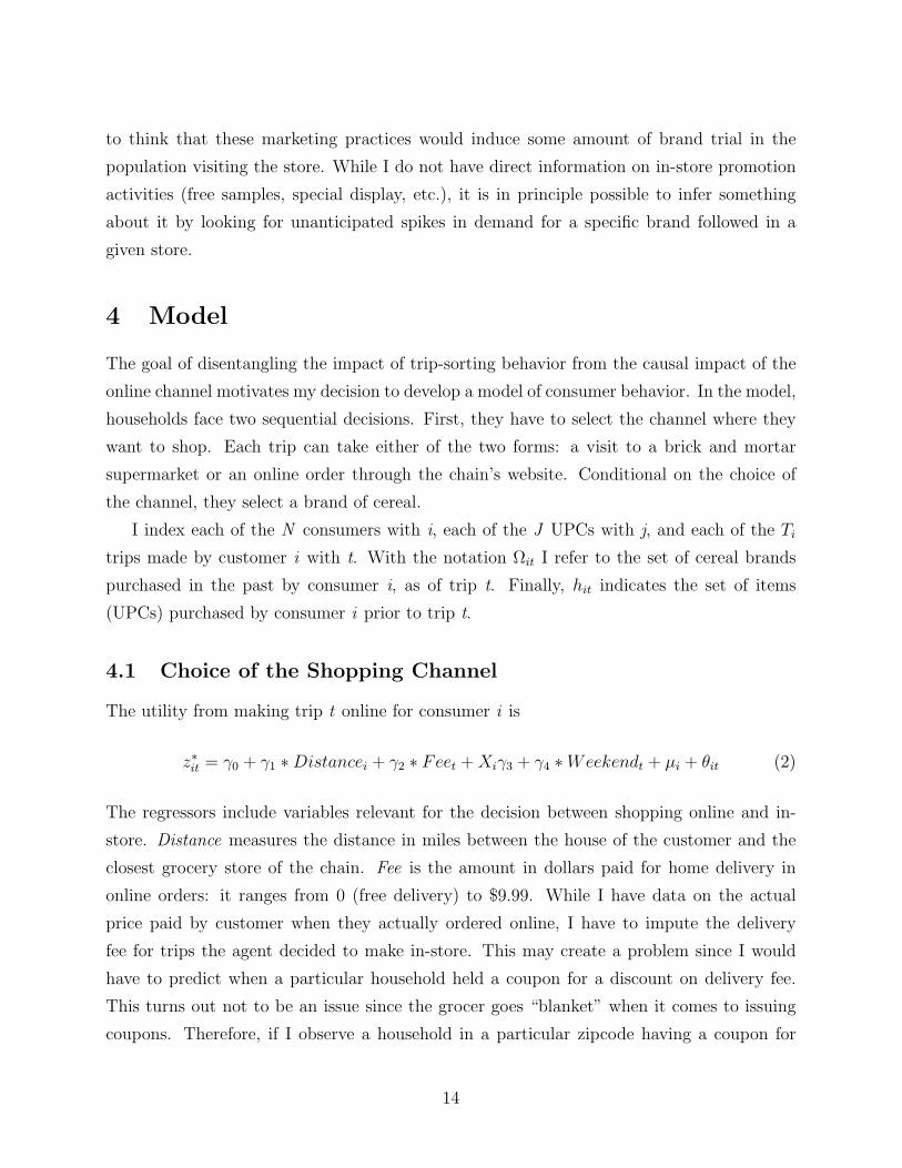
4 Model
The goal of disentangling the impact of trip-sorting behavior from the causal impact of the
online channel motivates my decision to develop a model of consumer behavior. In the model,
households face two sequential decisions. First, they have to select the channel where they
want to shop. Each trip can take either of the two forms: a visit to a brick and mortar
supermarket or an online order through the chain’s website. Conditional on the choice of
the channel, they select a brand of cereal.
I index each of the N consumers with i, each of the J UPCs with j, and each of the Ti
trips made by customer i with t. With the notation Ωit I refer to the set of cereal brands
purchased in the past by consumer i, as of trip t. Finally, hit indicates the set of items
(UPCs) purchased by consumer i prior to trip t.
4.1 Choice of the Shopping Channel
The utility from making trip t online for consumer i is
z∗it = γ0 + γ1 ∗Distancei + γ2 ∗ Feet +Xiγ3 + γ4 ∗Weekendt + µi + θit (2)
The regressors include variables relevant for the decision between shopping online and in-
store. Distance measures the distance in miles between the house of the customer and the
closest grocery store of the chain. Fee is the amount in dollars paid for home delivery in
online orders: it ranges from 0 (free delivery) to $9.99. While I have data on the actual
price paid by customer when they actually ordered online, I have to impute the delivery
fee for trips the agent decided to make in-store. This may create a problem since I would
have to predict when a particular household held a coupon for a discount on delivery fee.
This turns out not to be an issue since the grocer goes “blanket” when it comes to issuing
coupons. Therefore, if I observe a household in a particular zipcode having a coupon for
14

discount on delivery in a certain week, I can assume that every other customer living in the
same zipcode will have one too. The matrix Xi contains demographic information on the
household such as education, employment status and age of the head of the household. The
demographic variables are matched at the block group level from Census 2000. Weekend is
a dummy variable whose purpose is to capture the fact that time pressure is likely to be
lower in non working days. µi is a random effect that captures unobservable taste for online
trips by agent i. The random effect is distributed as follows
µi ∼ N(0, σµ) (3)
Moreover, it is independent from the i.i.d. shock θit which is a normally distributed dis-
turbance whose variance is normalized to 1. I observe the choice of the shopping channel
(where, with c=1, I refer to an online order) which follows the rule
c =
1 if z∗it ≥ 0
0 if z∗it < 0
4.2 Demand for Cereals
The utility consumer i derives from purchasing UPC j in trip t on channel c is modeled as
follows for in store purchases:
Uijt = β0 + β1Pricejt + βstore2 ∗ Ij /∈ hit+M storej + (δ + ξit) ∗ Ij /∈ Ωit+ vijt (4)
Similarly, for an online trip:
Uijt = β0 + β1Pricejt + βonline2 ∗ Ij /∈ hit+M onlinej + (δ + ξit) ∗ Ij /∈ Ωit+ vijt (5)
Price is the price per ounce paid by the household, net of discounts. The first indicator
function singles out UPCs consumer i never bought in the past. Therefore, β2 is the impact
on utility from purchasing a box of cereals whose UPC did not belong to the shopping history
of the household. I allow this effect to be different according to whether the consumer shops
online or in a store. Mj are UPC fixed effects, that are also interacted with the channel
dummy. The unobserved shock ξit only hits brands not experienced by the customer before,
instantaneous taste for variety.
15

The link between the two parts of the model is given by the generating process of the
unobserved shock ξit. I assume that the ξit and the θit, the disturbances in equation (2), are
jointly distributed according to a bivariate normal
(θ
ξ
)∼ BN
[(0
0
),Σ
]Σ =
[1 ρσξ
ρσξ σ2ξ
](6)
The parameter δ can be interpreted as the mean of the ξit shock. In some specifications, I
will parametrize it as follows
δ = α0 + α1Internet+ α2Weekend (7)
This allows the mean taste for new goods to fluctuate according to the channel selected and
the time of the week (weekend vs. weekday).
4.3 Discussion
The model tries to capture the relevant features presented in the descriptive section of the
paper. The potential bias deriving from sorting of trips across channels is addressed by al-
lowing θit and ξit to be correlated. This acknowledges the fact that unobserved determinants
of the choice of shopping online (e.g., lack of time) can, at the same time, also affect the
attitude towards brand experimentation.
Furthermore, I allow the impact on utility derived from purchase of a particular UPC
never bought in the past (β2) to be different for online and in-store trips. It is reasonable to
imagine that inertia in the choice of the UPC operates both online and in-store. Customers
tend to purchase the same box size or variety of their brand of choice. For this reason β2
should be negative in both channels. If the distaste for UPC never purchased before is only
driven by habits or unobservable characteristics, it should be equal for online and in-store
purchases. I attribute the additional stickiness in the choice of the UPC online (that is, the
difference between βonline2 and βstore2 ) to the effect of shopping on the online channel.
Two reasons for the channel choice to affect brand trial attitude have been presented
above. First, the online channel displays features, such as the shopping history list, that
lower the cost of repeated purchase relative to exploration. Moreover, exploration may be
perceived as more risky online because means of assessing quality of an unknown item are
limited. The model attempts to disentangle these explanations. As already pointed out, it is
16

possible to identify the two, exploiting variation in the amount of trials of new UPCs within
a given brand. This variation identifies βonline2 and βstore2 , which are informative on the value
of the shopping history feature. Allowing δ, the mean of the ξit shock, to vary according
to the channel, I capture structural differences in the taste for new brand for in-store and
Internet orders. One possible interpretation of this difference would be heterogeneous level
of uncertainty that makes exploration less attractive online.
5 Estimation
Below I describe the estimation procedure for the two components of the model: the selection
of the shopping channel (where we are estimating the vector of structural parameters γ), and
demand for cereals (whose parameters of interest are included in the vector β). The large
amount of observations at hand, and the importance of unobserved effects in the model make
it particularly appropriate to estimate it using Bayesian techniques. In a Gibbs sampling
approach, unobserved random effects are drawn from the appropriate distribution rather
than integrated out of the likelihood. This allows for significant gains in the estimation time
(Train, 2003). The description in the following paragraphs highlights the main features of
the procedure. Details are left to the appendix.
5.1 Channel selection: priors and sampling scheme
In order to estimate the channel selection probit in equation (2), I need to specify prior
distributions for the parameters of the model: the vector of coefficients γ, and the vector
of random effects µi. The last parameter of the model is variance of the distribution of the
random effects, σµ.
σµ ∼ IG(a1, a2) (8)
µ ∼ N(0, σ0µ) (9)
γ ∼ N(γ0, V0) (10)
a1, a2 are known hyperparameters. In particular, the prior on the inverse gamma is chosen
to be highly uninformative by setting a1 = 1 + 10−10, a2 = 1 + 10−5.
Sampling from the joint posterior of these parameters directly is challenging. Instead, I
apply the Gibbs sampling approach and make draws from the distribution of each parameter
at a time, conditioning on the values of the others. This turns out to be much simpler
17

and, after a sufficient number of iterations, the draws from the sequence of the conditional
distribution can be assumed to be draws from the joint posterior.
Given initial values for the parameters, the sampling scheme for each iteration is as follows
1. Apply data augmentation (Albert and Chib, 1993) to draw the z∗it from a normal
truncated distribution.
2. Draw γ from its full conditional distribution, a multivariate normal with mean γ and
covariance matrix V .
3. Draw µ from its full conditional distribution, a normal with mean zero and variance
σµ.
4. Draw σµ from its full conditional distribution, which is an inverse gamma.
5.2 Demand estimation: priors and sampling scheme
For the demand system, I assume a normal prior for the k-dimensional vector of coefficients
β. A prior is imposed over mean and variance of this normal distribution. The ξit unobserved
shocks are also parameters of the demand model. They are drawn from a bivariate normal
jointly with the errors of the channel selection equation as in equation (6). Therefore,
the final priors to be specified refer to the mean of the random effect and to the variance
covariance matrix of the bivariate normal.
β ∼ N(b,W ) (11)
Σ ∼ IW (2, I) (12)
Once again, I simulate draws from the joint posterior of the parameters by sampling from
their conditional distributions. Each iteration of the sampler unfolds as follows
1. Draw β from its conditional distribution
π(β|yit, ξit) ∝ L(yit|β, ξit)
Draws from this distribution are approximated with draws from a normal and the trial
values are accepted or rejected using a Metropolis-Hastings algorithm.
2. Draw ξit jointly with θit from the distribution specified in equation (6).
18

3. Draw Σ from an inverse Wishart.
4. Obtain δ by simple OLS.
6 Results
The model is estimated using a random subsample of 500 households9, for a total of 2,778
trips, 783 of which are online orders. Results are displayed in Table 9 and Table 10 for
channel selection and demand respectively.
As we would expect, the higher the fee charged for home delivery the less appealing it is
to shop on the Internet. The coefficient on the weekend dummy is negative and very large
(the implied elasticity is 57%). It reflects the low incentive to shop online during weekends,
when agents have more free time to do their shopping. This reinforces the idea that shocks
to the utility of time play a role in affecting the selection of the shopping channel. A similar
interpretation can be given to the positive impact of income on the probability of shopping
online. Customers also tend to prefer the online channel when they live further away from
the closest grocery store of the chain, consistently with findings in the literature (Chiou,
2008). The variables related to age enter with negative coefficient, which is expected as the
excluded group age is 18 to 35 years, that is the youngest and most likely to be at ease with
technology.
The demand step is estimated under different specifications. In columns I and II in Table
10 I impose δ, the mean of the shock to the taste for new brands ξ, to be the same for each
trip. I relax this assumption in the estimates presented in columns III and IV, where δ
is parametrized as in equation (7). The coefficient on price is negative and similar in all
the specifications. Column II and IV include an interaction between the price variable and
the channel to assess the existence of different prince sensitivity for online purchase. This
interaction enters with positive sign10 implying that customers are less price sensitive when
shopping online. While some of the literature has found the opposite (Brynjolfsson and
Smith, 2000; Ellison and Ellison, 2001), my result is in line with other studies of the grocery
sector (Chu, Chintagunta, and Cebollada, 2008; Andrews and Currim, 2004). The difference
9This is aimed at saving computation time. Given the large number of brands included in my analysis,each shopping situation implies listing of covariates for more than 100 brands. This requires to limit thenumber of trips taken into consideration to avoid the matrix of regressors from growing too large and slowingdown the estimation routine.
10However only 73% of the draws are positive.
19
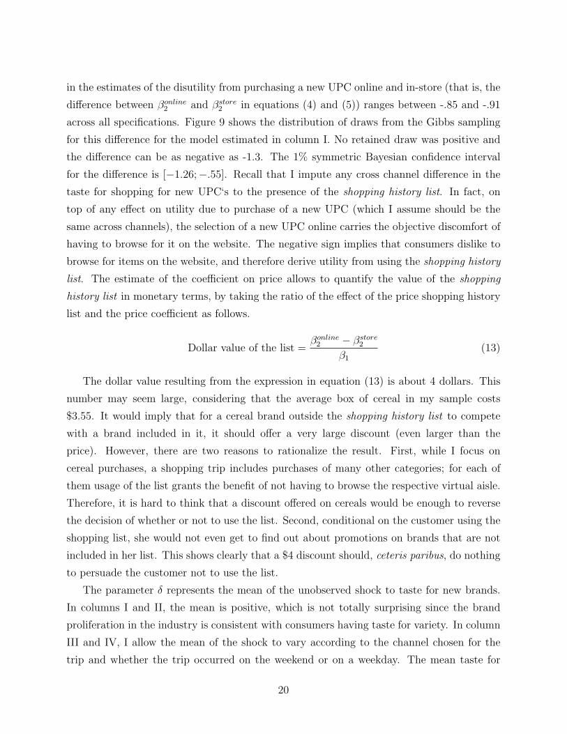
in the estimates of the disutility from purchasing a new UPC online and in-store (that is, the
difference between βonline2 and βstore2 in equations (4) and (5)) ranges between -.85 and -.91
across all specifications. Figure 9 shows the distribution of draws from the Gibbs sampling
for this difference for the model estimated in column I. No retained draw was positive and
the difference can be as negative as -1.3. The 1% symmetric Bayesian confidence interval
for the difference is [−1.26;−.55]. Recall that I impute any cross channel difference in the
taste for shopping for new UPC‘s to the presence of the shopping history list. In fact, on
top of any effect on utility due to purchase of a new UPC (which I assume should be the
same across channels), the selection of a new UPC online carries the objective discomfort of
having to browse for it on the website. The negative sign implies that consumers dislike to
browse for items on the website, and therefore derive utility from using the shopping history
list. The estimate of the coefficient on price allows to quantify the value of the shopping
history list in monetary terms, by taking the ratio of the effect of the price shopping history
list and the price coefficient as follows.
Dollar value of the list =βonline2 − βstore2
β1
(13)
The dollar value resulting from the expression in equation (13) is about 4 dollars. This
number may seem large, considering that the average box of cereal in my sample costs
$3.55. It would imply that for a cereal brand outside the shopping history list to compete
with a brand included in it, it should offer a very large discount (even larger than the
price). However, there are two reasons to rationalize the result. First, while I focus on
cereal purchases, a shopping trip includes purchases of many other categories; for each of
them usage of the list grants the benefit of not having to browse the respective virtual aisle.
Therefore, it is hard to think that a discount offered on cereals would be enough to reverse
the decision of whether or not to use the list. Second, conditional on the customer using the
shopping list, she would not even get to find out about promotions on brands that are not
included in her list. This shows clearly that a $4 discount should, ceteris paribus, do nothing
to persuade the customer not to use the list.
The parameter δ represents the mean of the unobserved shock to taste for new brands.
In columns I and II, the mean is positive, which is not totally surprising since the brand
proliferation in the industry is consistent with consumers having taste for variety. In column
III and IV, I allow the mean of the shock to vary according to the channel chosen for the
trip and whether the trip occurred on the weekend or on a weekday. The mean taste for
20
variety is lower on the Internet, possibly capturing the higher uncertainty over quality faced
in online exploration. The parameter α2 is positive, implying that customers are more likely
to value new brands on weekends. This would be the case if, for example, parents are more
likely to shop with children during weekends, as children are well known source of brand
switching. Finally, ρ, the correlation between the unobserved shock to new brands ξit and
the residual from the shopping channel selection is negative, although small. Large shocks to
the instantaneous utility of time (which drive the agent to shop online) are associated with
small or negative shocks to the taste for new brands. This is consistent with the view that
online trips are more likely to be made in instances when utility of time is higher, which are
likely to be occasions where there is little time to think of exploring new brands.
To assess the fit of my model, I compare the Lorenz curve obtained with simulation from
my estimates with the one resulting from actual data.11 Figure 10 and 11 shows the fit for
brands and for cereal manufacturers, respectively. At the brand level, the model slightly
overpredicts concentration on both channels. Still a main stylized fact of the original data
is preserved: bigger manufacturers and most popular brands display higher market share
for purchases made online. As we would have expected, at the greater level of aggregation
the fit improves: at the manufacturer level Lorenz curves from actual and fitted data almost
perfectly overlap.
7 Counterfactual exercises
In this section, I run counterfactual experiments in order to understand the practical impli-
cations of the estimates of the structural model. In each counterfactual, the initial shopping
history of each agent is based on their purchases in the first three months of data (which are
therefore not used for the simulation, just as they were not for the estimation). Then, after
each trip, the shopping list of the customer is updated to include any eventual new brand
she could have picked. The parameters used for the simulations are the ones resulting from
the specification III in Table 10. The results I presented are averages over 1,000 simulations.
11Brynjolfsson, Hu, and Simester (2006) use the Lorenz curve to describe the level of concentration of anindustry. In my case, I use the degree at which my simulated Lorenz curve matches the actual one as asynthetic measure of predictive power of the model.
21

7.1 The amount of exploration
My focus in the counterfactuals is on the impact of the past shopping history list. Of all
the features I included in the model, the effect of the list has certainly the highest practical
relevance both to the players in the industry and to the policy makers. In fact, its existence
depends on a choice about the design of the website which is completely under the control of
the retailer. Much unlike those of instantaneous shocks to the utility of time and of the gap
in the ability to assess new items, the effect of the past shopping history list can be removed
or reshaped by modifying the layout of the website.12
The shopping history list reduces the cost of shopping, by lowering the effort needed for a
repeated purchase. This makes brand exploration less attractive in the online environment;
I am interested in a quantification of this effect. How much extra brand exploration would
take place on the online channel if the past shopping history list feature were not available?
Recall that I interpret the difference in the estimate of βonline2 and βstore2 as the effect of the
list. Therefore, simulating a world where the list does not exist implies running the model
setting βonline2 at the same level as βstore2 . This results in the total number of brand trials in
online purchases over the two years increasing by 23%. However, in levels, the amount of
brand exploration online is still lower than in the store.
7.2 Lock-in effect
While evaluating the change in the amount of exploration after removing the list is infor-
mative about the magnitude of its effect, it is not a sharp enough exercise to understand its
importance. By definition, the most popular brands will already be in the initial shopping
history for a large number of my consumers. As a result, most of the exploration is towards
brands in the fringe of the market. It is interesting to ask to what extent being forced out
of the list would affect the success of an otherwise popular brand.
To simulate this scenario, I selected General Mills’ Cinnamon Toast Crunch, a brand
with large in-store sales and even more popular online. I modified the initial shopping
histories of all consumers so that Cinnamon Toast Crunch is in nobody’s past shopping
history list. It can be noticed that this exercise amounts to simulating the entry of a new
brand looking exactly as Cinnamon Toast Crunch (same price and characteristics) but lacking
12Lewis (2007) argues that extensive use of text and pictures, as measured by megabytes allocated tothe description of an item, can reduce information asymmetries in the case of a buyer unable to personallyinspect a car. In this spirit, some design changes could also have the effect of reducing the gap in theuncertainty over new brands.
22

any installed base.13 Therefore, results from this counterfactual can also be interpreted as
an evaluation of the difference in entry barriers online and in-store faced by a new entrant.
In this context, Cinnamon Toast Crunch starts without any loyal customer: it is reasonable
that its market share will be lower than the one held by the same brand in the baseline
model on both channels. As time goes by, market shares should catch up with the baseline.
However, purchase of the “unknown” brand is less appealing online because of the extra
cost attributable to browsing. Therefore, it could be the case that the catch up between
the counterfactual and baseline market shares for Cinnamon Toast Crunch is slower on the
Internet channel. The difference in the rate of catch-up is informative on the magnitude of
entry barriers generated by the design of the website.
Figure 12 compares Cinnamon Toast Crunch’s market shares under the baseline model
and the counterfactual on both distribution channels. At first, the counterfactual market
share is lower than in the baseline, both online and in-store. The figures tend then to converge
over time; however this catch-up is faster in-store. Figure 13 compares the percentage of the
baseline market share reached in the counterfactual brand over time on the two channels.
While the catch-up is homogeneous in the first semester, eventually the counterfactual brand
reaches more than 60% of its “target” market share in store but never exceeds 40% of it
online. The single difference between the two environment is that a new brand, on top of
any entry barrier it faces in-store (quantified by the level of βstore2 in my estimates) faces the
additional effect of the list (the difference between βonline2 and βstore2 ) on the Internet channel.
The result is even more striking since the wedge caused by the list manages to slow down
adoption of a brand that was fairly well liked by consumers to begin with.
7.3 Contextual advertising/Recommendations
Contextual advertising and customer recommendations are popular form of advertising and
customer loyalty enhancing for online businesses. Context ads are individually targeted
promotion based on the content of the page the consumer is browsing. For example, they
are regularly displayed along with results from a search on a search engine. Somewhat
similarly, recommendation systems are suggestions that the firm offers to a customer based
on her previous shopping history. The firm uses purchases by other customers with similar
shopping history to forecast goods or offers that may be of interest to her. This system has
13To be precise, the exercise simulates the entry of such a brand in a world where Cinnamon Toast Crunchdid not exist.
23

been made popular by Amazon.com and Netflix.
I can simulate the effect of the introduction of a particular form of context ads in the
website of the grocery chain I am studying. I assume that, while looking at their shopping
history list, consumers will be given a recommendation for a cereal brand that is not part of
it. In my exercise, the advertising message will promote the same brand to all the consumers
and will be displayed as a popup or a direct link both in the main page of the website and
in the shopping history list. Figure 14 shows what the customer would see on her screen if
a context ad were to be added to the shopping history list. In the same screen with the list
of already purchased brand, the customer can observe (on the right) a recommendation of
another brand she has not purchased before. The advantage of brands belonging to the list
was to be “just one click away” for the consumer. Thanks to the recommendation, now even
an unknown brand can be as easy to purchase.
The implementation of this counterfactual consists in a variation of the one presented in
the previous section. Once again, I remove Cinnamon Toast Crunch from the brand history
of every household (making it look like a new entrant). However, I simulate the effect of a
recommendation box advertising Cinnamon Toast Crunch to each customer when she shops
online. In practice, I remove the effect of the list by setting βonline2 at the same level as
βstore2 but only for the Cinnamon Toast Crunch brand. This means that the effort required
to a household in order to purchase Cinnamon Toast Crunch, is the same as the one needed
to purchase another brand already part of the household’s shopping history list. Figure 15
shows the ratio between market share in the counterfactual and in the baseline simulation
over time for the two channels. The convergence to the benchmark market share evolves
pretty much like in the previous experiment for in-store sales; there is a marked difference for
the results on the online channel. Online market share for the new introduced brand reaches
the same level (actually slightly exceeds it) as in the baseline model in the first semester.
Therefore, with the help of a recommendation system, it would take less than six months
for Cinnamon Toast Crunch to make up for the disadvantage of being stripped of its initial
share of loyal customers. Moreover, the online market share in the counterfactual stabilizes
at a level 50% higher than the one held in the baseline on the same channel. This suggests
that not only the context ad helps the brand to regain its customer base but also attracts
new customers.
24
8 Conclusions
In this paper, I focus on how the choice of the shopping channel affects households’ propensity
to try brands they have not tried before. After documenting that brand exploration is
more prominent in-store than online, I investigate the role of three different mechanisms
that can explain this result. I do so by developing and estimating a structural model of
consumer behavior that allows me to quantify their importance. My estimates suggest that
cost of browsing plays a relevant role in explaining while shoppers are more averse to brand
exploration when they transact online and can be quantified in about $4. Some of the lower
attitude towards exploration for online trips is also explained by the correlation between the
taste for exploration and specific circumstances that drive the decision of shopping for grocery
online. It is important to identify this component because, unlike the other mechanisms I
am interested in, it is not due to a causal effect of the Internet channel on behavior. In my
counterfactuals, I simulate the effect of eliminating the cost of browsing. This results in a
23% increase in the level of brand exploration online. Also, I assess the degree to which the
implied lock-in represents a barrier to entry online by simulating the introduction of a new
cereal brand. I compare its performance to a case where the entry barriers it faces are lower
due to the existence of an installed base of customers. Convergence of the new brand to its
“natural” market share is 20% lower online than it is in store. Finally, I find that adoption
of features such as context ads and recommendations on the grocer ’s website would have
the potential of reversing this effect, making it easier for the “outsiders” to become popular
online.
My analysis suggests that brands that are unpopular in-store may find it even harder to
gain ground online. In fact, online customers seem to be willing to give up consumption of
very well liked brands, if they were to drop out of their shopping history list. My last coun-
terfactual suggests that a potentially successful strategies for manufacturers of new brands
include trying to overcome the disadvantage in terms of the extra cost of browsing needed
to reach them (e.g. getting pop-up ads or link on the main page after login). Alternatively,
it may be advisable to try and “win the battle in the store”. For example obtaining visible
slots on the shelves, couponing, or organizing in-store trials.
The main policy implication of my results relates to entry barriers. Conventional wisdom
has it that the Internet removes traditional sources of switching cost and monopoly power (i.e.
location advantage), making competition fiercer and lowering barriers to entry. However, I
show in my application that it is possible for online commerce to have an opposite effect,
25

introducing new barriers of its own. For non established brands, it is actually harder to
receive attention from customers online than in the store. In this sense, the Internet does
not look at all as a threat to the dominant position of the incumbents. This by no means
implies that the paradigm of the “frictionless commerce” has to be rejected. My findings
stress the necessity of thinking about the impact of online shopping taking into account not
only the characteristics of each industry, but also the specific fashion in which the service is
provided to the customers. These details can have a significant impact and ultimately affect
consumers’ behavior in ways that would appear counterintuitive at a more superficial level
of analysis.
26

References
Aguiar, M., and E. Hurst (2007): “Life-Cycle Prices and Production,” American Eco-
nomic Review, 97(5), 1533–1559.
Albert, J. H., and S. Chib (1993): “Bayesian analysis of binary and polychotomous
response data.,” Journal of the American Statistical Association, 88(422), 669–.
Andrews, R. L., and I. S. Currim (2004): “Behavioral Differences between Consumers
Attracted to Shopping Online vs. Traditional Supermarkets: Implications for Enterprise
Design and Strategy,” International Journal of Marketing and Advertising, 1(1), 38–61,
working paper.
Bakos, J. Y. (1997): “Reducing Buyer Search Costs: Implications for Electronic Market-
places,” Management Science, 43(12), 1676–1692.
Bhatnagar, A., S. Misra, and H. R. Rao (2000): “On Risk, Convenience, and Internet
Shopping Behavior.,” Communications of the ACM, 43(11), 98–105.
Brown, J. R., and A. Goolsbee (2002): “Does the Internet Make Markets More Com-
petitive? Evidence from the Life Insurance Industry,” The Journal of Political Economy,
110(3), 481–507.
Brynjolfsson, E., Y. J. Hu, and D. Simester (2006): “Goodbye Pareto Principle,
Hello Long Tail: The Effect of Search Costs on Concentration of Product Sales,” MIT
Center for Digital Business Working Paper.
Brynjolfsson, E., and M. D. Smith (2000): “Frictionless Commerce? A Comparison
of Internet and Conventional Retailers.,” Management Science, 46(4), 563–.
Brynjolfsson, E., M. D. Smith, and A. Montgomery (2004): “The Great Equalizer?
An Empirical Study of Consumer Choice at a Shopbot,” MIT Sloan School mimeo.
Burke, R. R., B. A. Harlam, B. E. Kahn, and L. M. Lodish (1992): “Comparing
Dynamic Consumer Choice in Real and Computer-simulated Environments.,” Journal of
Consumer Research, 19(1), 71–82.
Chevalier, J., and A. Goolsbee (2003): “Measuring Price and Price Competition On-
line: Amazon and Barnes and Noble,” Quantitative Marketing and Economics, 1(2), 203–
222.
27

Chiou, L. (2008): “Empirical Analysis of Competition between Wal-Mart and Other Retail
Channels,” Journal of Economics and Management Strategy, forthcoming.
Chu, J., P. Chintagunta, and J. Cebollada (2008): “A Comparison of Within-
Household Price Sensitivity across Online and Offline Channels,” forthcoming in Mar-
keting Science.
Clemons, E. K., I.-H. Hann, and L. M. Hitt (2002): “Price Dispersion and Differ-
entiation in Online Travel: An Empirical Investigation.,” Management Science, 48(4),
534–549.
Danaher, P. J., I. W. Wilson, and R. A. Davis (2003): “A Comparison of Online and
Offline Consumer Brand Loyalty.,” Marketing Science, 22(4), 461–476.
Degeratu, A. M., A. Rangaswamy, and J. Wu (2000): “Consumer choice behavior in
online and traditional supermarkets: The effects of brand name, price, and other search
attributes.,” International Journal of Research in Marketing, 17(1), 55–78.
Dube, J. P., G. Hitsch, and P. Rossi (2008): “Do Switching Costs Make Markets Less
Competitive?,” Journal of Marketing Research, forthcoming.
Einav, L., E. Leibtag, and A. Nevo (2008): “Not-so-classical measurement errors: a
validation study of Homescan,” working paper.
Ellison, G., and S. Ellison (2001): “Search, Obfuscation, and Price Elasticities on the
Internet,” working paper, MIT.
Goettler, R. L., and K. Clay (2006): “Tariff Choice with Consumer Learning:Sorting-
Induced Biases and Illusive Surplus,” working paper.
Goolsbee, A. (2001): “Competition in the Computer Industry: Online versus Retail,” The
Journal of Industrial Economics, 49(4), 487–499.
Hann, I.-H., and C. Terwiesch (2003): “Measuring the Frictional Costs of Online Trans-
actions: The Case of a Name-Your-Own-Price Channel.,” Management Science, 49(11),
1563–1579.
Jin, G., and E. Kato (2007): “Dividing Online and Offline: A Case Study,” working
paper.
28

Lewis, G. (2007): “Asymmetric Information, Adverse Selection and Seller Disclosure: The
Case of eBay Motors,” working paper.
Mazar, N., A. Herrmann, and E. J. Johnson (2007): “Preferences and choice behavior
online: A cognitive cost approach to understanding product class differences,” working
paper.
Nevo, A., and C. Wolfram (2002): “Why Do Manufacturers Issue Coupons? An Em-
pirical Analysis of Breakfast Cereals,” RAND Journal of Economics, 33(2), 319–339.
Pozzi, A. (2007): “Channel Selection and Basket Characteristics,” working paper.
Scherer, F. M. (1979): “The Welfare Economics of Product Variety: An Application to
the ready-to-eat Cereals Industry.,” Journal of Industrial Economics, 28(2), 113–134.
Schmalensee, R. (1978): “Entry deterrence in the ready-to-eat breakfast cereal industry.,”
Bell Journal of Economics, 9(2), 305–327.
Shin, S., S. Misra, and D. Horsky (2007): “Disentangling Preferences, Inertia and
Learning in Brand Choice Models,” working paper.
Shum, M. (2004): “Does Advertising Overcome Brand Loyalty? Evidence from the
Breakfast-Cereal Market,” Journal of Economics and Management Strategy, 13(2), 241–
272.
Train, K. (2003): Discrete Choice Methods with Simulation. Cambridge University Press.
29

Appendix
A Estimation
Details related to the estimation routine presented in Section 5 are discussed below.
A.1 Selection of the Shopping Channel
Draw of the z∗it
The distributional assumption made over the θit in equation (6), implies that the z∗it are
distributed according to a truncated normal with mean Citγ + µi and variance 1. The
support is (−∞, 0] if the trip occurs in a store, and [0,+∞) if the trip is made online.
Draw of γ
The full conditional posterior on γ is normal with mean γ and variance matrix V . Given
the analogy with the posterior for regression parameters in a linear model, we have
γ ∼ N((C ′C)−1C ′Z∗, (C ′C)−1) (14)
where Z∗ is the vector of the stacked z∗it.
Draw of µ
For each agent, the random effect µi is drawn from a normal distribution with mean 0 and
variance σµ.
Draw of σµ
The density of σµ conditional on the other parameters is an inverse gamma distribution,
IG(a1, a2), where
a1 =NI + 2a1
2(15)
a2 =
∑Ii=1 µ
2i + 2a2
(2 + I)(16)
30

where I is the total number of random effects to be drawn.
A.2 Demand for Cereals
Draw of βi’s
Each of the βi should be drawn from the conditional density
π(β|yit, ξit) ∝∏t
∏j
(exp(xijtβ + ξit)∑j exp(xijtβ + ξit)
)Iyit=j
(17)
= L(yit|β, ξit)
Once again, sampling from this distribution is not easy. Therefore, I adopt a Metropolis-
Hastings procedure. The vector of coefficient is drawn from a normal distribution and the
draws are then accepted or rejected in fashio similar to the one explained for the draws of
the µ above.
Draw of ξit’s
Draws of the time-individual specific shocks to the valuation of unknown brands are made
jointly with the simulation of the residuals from the channel selection probit. Standard
Choleski transformation allows to draw from their joint distribution, specified in (6). These
draws of ξit, however, have to be considered as trial values whose acceptability has to be
assessed through updating with the data. In particular
π(ξit|yit, β, δ,Σ) ∝ φ(ξit|ρ, σξ, θit) ∗∏t
∏j
(exp(xijtβ + ξit)∑j exp(xijtβ + ξit)
)Iyit=j
(18)
= φ(ξit|ρ, σξ, νit) ∗ L(yit|β, ξit)
where φ(ξit|ρ, σξ, θit) has mean δ+ ρσξθit, and variance 1− ρ. The density in equation (18) is
used to evaluate draws from the bivariate truncated in (6) in a Metropolis-Hastings routine.
31

Computation of δ
In every iteration, δ is computed as
δ = 1/R∑i
∑t
(ξit − ρθit) (19)
with R being the total number of trips in the sample.
In the specifications where δ is parametrized as in equation (7), the parameter are recovered
by running OLS on
(ξit − ρθit) = α0 + α1Internet+ α2Weekend (20)
Draw of Σ
The variance-covariance matrix of the bivariate truncated is drawn from an inverse Wishart
distribution with 2+R degrees of freedom and scale matrix
2I +RΣ
2 +R(21)
where Σ is the variance matrix implied by the draws of θit and ξit in that iteration.
32

Tables and Figures
Table 1: Trip descriptive statistics by channel of purchase, for all the trips.
All trips Large tripsIn store Online P-value In store Online P-value
Total expenditure 45.31 151.99 .000 162.16 179.70 .000
Basket size 15.15 55.61 .000 69.59 77.85 .000
Number of unique items 11.35 34.34 .000 62.41 63.05 .000
Total expenditure is net of any discount and is expressed in dollars. The total number ofin-store trips is 1,662,375; while the total number of online orders is 166,879. Basket sizerefers to the total number of items purchased in the trip; as opposed to the number ofunique item, that does not double count multiple purchases of the exact same item. “Largetrips” are defined as trips worth more than 100 dollars (212,946 in store trips and 122,320online), when comparing total expenditure; or trips with a basket size of at least 50, whencomparing basket size (116,236 in store trips and 84,148 online); or trips at least 50 uniqueitems purchased, when comparing number of unique items (49,061 in store trips and 28,196online). The P-values refer to a t-test for the equality of means.
33
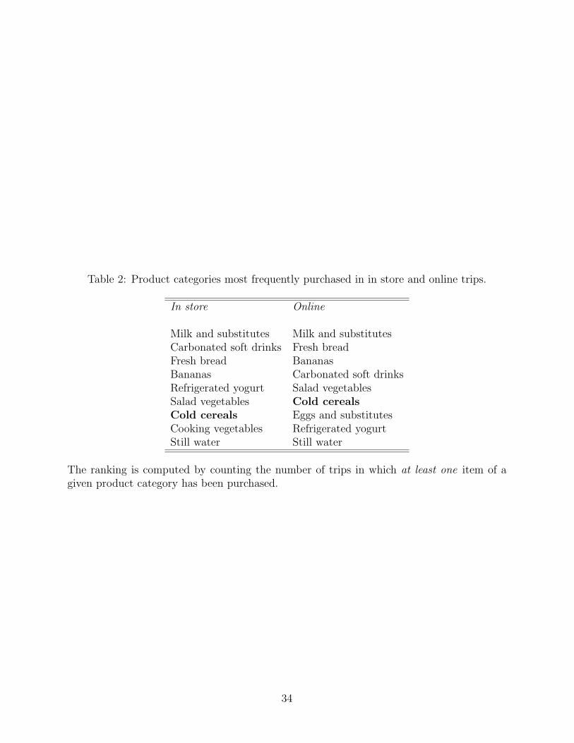
Table 2: Product categories most frequently purchased in in store and online trips.
In store Online
Milk and substitutes Milk and substitutesCarbonated soft drinks Fresh breadFresh bread BananasBananas Carbonated soft drinksRefrigerated yogurt Salad vegetablesSalad vegetables Cold cerealsCold cereals Eggs and substitutesCooking vegetables Refrigerated yogurtStill water Still water
The ranking is computed by counting the number of trips in which at least one item of agiven product category has been purchased.
34

Table 3: Trip descriptive statistics by channel of purchase, for all the trips involving purchaseof breakfast cereals.
In store OnlineTotal expenditure 110.83 179.24
(78.61) (89.53)
Basket size 40.51 66.29(27.77) (35.12)
Number of unique items 30.56 41.56(20.03) (19.04)
Number of unique categories 23.29 30.42(14.36) (12.65)
Number of cereal boxes 1.52 1.88(.8913) (1.49)
Number of unique cereal brands 1.26 1.40(.5640) (.8043)
Number of obs. 106,378 35,647
Total expenditure is net of any discount and is expressed in dollars. Basket size refers to thetotal number of items purchased in the trip; as opposed to the number of unique item thatdoes not double count multiple purchases of the exact same item. Standard deviations arereported in parentheses.
35

Table 4: Demographic information.
5th 25th 50th 75th 95th
percentile percentile percentile percentile percentileNumber of trips 43.8 96 158 245 449.2Number of cereal trips 3 10 21 36 68Share trips online (%) .4 1.7 5.6 16.7 53.6Share cereal trips online (%) 0 1.4 12.5 40 .91Black 0 .2 1.7 4.5 19.7Hispanic .4 3.8 7.4 14.4 36.6College degree 18.8 35 49.6 63.2 78.7Employed 49.7 60.4 66.7 71.9 79.2Per capita income 16,261 23,837 30,791 41,884 69,045Commute ≤ 30 min 36.18 49.3 57.3 66 79.3Commute 30 to 59 min 14.7 25.1 32.2 38.6 49.3Commute > 60 min 1.5 5 8.9 14.3 23.715 < Age < 35 0 4.6 9.7 17 31.635 ≤ Age < 54 27.1 44.5 53.6 62.5 75.154 ≤ Age < 65 0 10.4 16.1 22.1 32.9Age ≥ 65 0 8.2 15.8 25 42.2Distance .26 .65 1.09 1.72 3.38
Information on number of trip, number of cereal trips and number of online trips are con-structed from the scan data provided from the grocer. Distance is the geodesic distance inmiles between the domicile of the household and the closest brick and mortar store of thesupermarket chain and was also provided by the retailer. the 6,021 whose demographicsare available. All the other variables (black, hispanic, college degree, employed, per capitaincome, age and commuting time) are matched from Census 2000 at the block group levelfor the 6,021 households for which 9-digit zipcode of residency was provided.
36

Table 5: Average number of brand trials for in-store vs. online trips.
In store Online P-valueAll trips .3576 .2593 .000
(.0013) (.0019)
Trips worth > $100 .3517 .2600 .000(.0018) (.0020)
Basket size > 50 .3568 .2652 .000(.0030) (.0034)
Brand trial is defined as purchase of a brand not bought in the previous three months. P-values refer to t-test where the null hypothesis is equality of the means. Standard errors arereported in parenthesis.
37
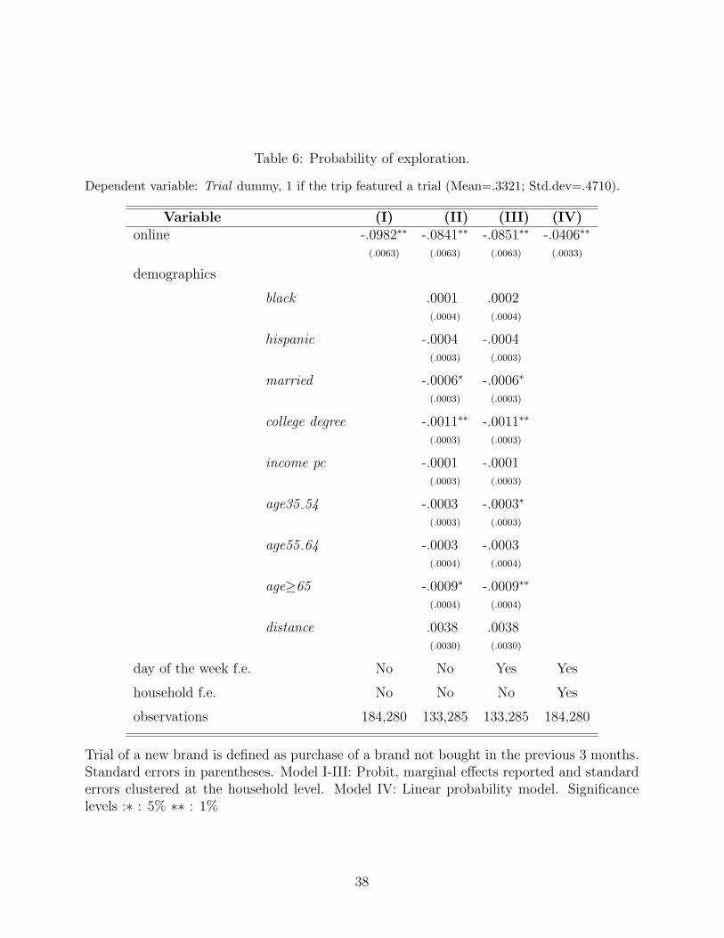
Table 6: Probability of exploration.
Dependent variable: Trial dummy, 1 if the trip featured a trial (Mean=.3321; Std.dev=.4710).
Variable (I) (II) (III) (IV)online -.0982∗∗ -.0841∗∗ -.0851∗∗ -.0406∗∗
(.0063) (.0063) (.0063) (.0033)
demographics
black .0001 .0002(.0004) (.0004)
hispanic -.0004 -.0004(.0003) (.0003)
married -.0006∗ -.0006∗
(.0003) (.0003)
college degree -.0011∗∗ -.0011∗∗
(.0003) (.0003)
income pc -.0001 -.0001(.0003) (.0003)
age35 54 -.0003 -.0003∗
(.0003) (.0003)
age55 64 -.0003 -.0003(.0004) (.0004)
age≥65 -.0009∗ -.0009∗∗
(.0004) (.0004)
distance .0038 .0038(.0030) (.0030)
day of the week f.e. No No Yes Yes
household f.e. No No No Yes
observations 184,280 133,285 133,285 184,280
Trial of a new brand is defined as purchase of a brand not bought in the previous 3 months.Standard errors in parentheses. Model I-III: Probit, marginal effects reported and standarderrors clustered at the household level. Model IV: Linear probability model. Significancelevels :∗ : 5% ∗∗ : 1%
38

Table 7: Average number of UPC switches, for online vs. in-store trips.
In store OnlineSame brand, same UPC 56,296 29,630
(65.1%) (79.66%)
Same brand, different UPC 30,177 7,563(34.9%) (20.34%)
Frequency of purchase of a new UPC, conditional on purchase of a known brand, acrosschannels. Only trips in which the household bought a known brand are considered.
39

Table 8: Probability of purchasing a new UPC.
Dep. var: New upc, equal to 1 if the upc purchased had not been previously bought (Mean=.0839std.dev=.2773).
Variable (I) (II)online -.0352∗∗∗ -.0349∗∗∗
black -.0002∗
hispanic -.0001
college degree -.0004∗∗∗
employed .0001
income pc .0004
age35 54 .0001
age55 64 .0002∗∗∗
age≥65 -.0001
observations 123,766 123,766
Only trip resulted in purchase of already known brands are considered. Model I-II: probit,marginal effects are reported. Significance levels :∗ : 10% ∗∗ : 5% ∗ ∗ ∗ : 1%
40

Table 9: Channel selection equation estimates.
Dep. var.: 1 if the trip is made online (mean=.2798, st.dev=.4489).
items count .0002 income per cap .0049(.0002) (.0004)
distance .0087 age35 54 -.0030(.0009) (.0002)
fee -.1001 age55 64 -.0071(.0006) (.0003)
weekend -.4929 age≥65 -.0028(.0002) (.0002)
married -.0086 college -.0036(.0001) (.0045)
employed -.0003 σµ .124(.0003) (.0011)
The unit of observation is a trip (2,778 trips). Burn-in period: 1000 draws, mean andstandard deviation of the posterior are computed on the basis of the next 1000 draws.
Marginal effects reported.
41

Table 10: Demand estimates.
Variable (I) (II) (III) (IV)price -.21 -.22 -.20 -.22
(.0206) (.0248) (.0215) (.0239)
price*Internet .09 .08(.0488) (.0497)
Ij /∈ hit ∗Onlinet (βonline2 ) -6.96 -7.01 -6.84 -6.88(.1247) (.1340) (.1187) (.1333)
Ij /∈ hit ∗ (1−Onlinet) (βstore2 ) -6.11 -6.11 -5.97 -5.97(.0661) (.0695) (.0661) (.0646)
δ .93 .94(.0487) (.0474)
α0 1.26 1.26(.0261) (.0271)
α1 -.69 -.69(.1661) (.1566)
α2 .07 .07(.0373) (.0372)
σξ .13 .86 .67 .18(.0007) (.0015) (.0011) (.0009)
ρ -.01 -.02 -.01 -.01(.0076) (.0083) (.0079) (.0081)
The unit of observation is a cereal trip (2,778 observations). Standard deviation of the poste-rior is reported in parenthesis. Burn-in period: 1000 draws, mean and standard deviation ofthe posterior are computed on the basis of 2500 draws of which 1 out of 10 is retained. UPCfixed effects are included in the specification and interacted with the channel dummy. ρ isthe correlation between the residuals of the channel selection equation and the unobservedshock to utility derived from new brands. δ is the mean of the unobserved shock to utilityderived from new brands, which is estimated as a parameter in column I and II. In columnIII and IV, δ is assumed to be a function of the channel and of the time of the trip and thecoefficients of this parametrization α0, α1, α2 are reported.
42

0.1
.2.3
.4
0 2.95 3.95 4.95 5.95 6.95 7.95 8.95 9.95Fee paid
Figure 1: Frequency distribution of delivery fees (in dollars) paid in online orders.
Figure 2: Screenshot from the grocer ’s website.
43

Figure 3: Screenshot from the grocer ’s website: shopping by aisle.
Figure 4: Structure of the data: brand vs. UPC.
44

Figure 5: Coefficient on the Online dummy from estimation of equation 1, for differentdefinitions of the dependent variable, across specifications. The picture compares coefficientsresulting from defining trial as purchase of a brand not bought in the x months before. Wherex is set to 2, 3, 4, 6 months or a year. The resulting coefficient is normalized by the meanof the dependent variable to allow for comparison.
45
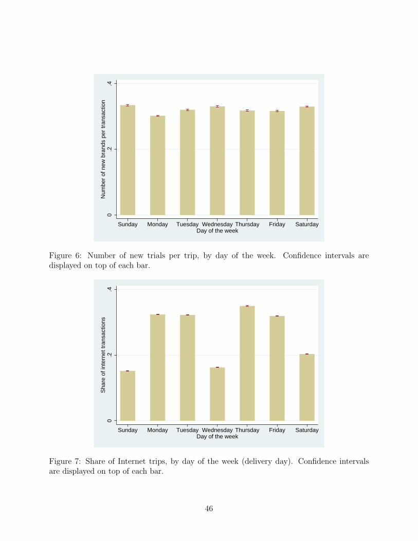
0.2
.4N
umbe
r of
new
bra
nds
per
tran
sact
ion
Sunday Monday Tuesday Wednesday Thursday Friday SaturdayDay of the week
Figure 6: Number of new trials per trip, by day of the week. Confidence intervals aredisplayed on top of each bar.
0.2
.4S
hare
of i
nter
net t
rans
actio
ns
Sunday Monday Tuesday Wednesday Thursday Friday SaturdayDay of the week
Figure 7: Share of Internet trips, by day of the week (delivery day). Confidence intervalsare displayed on top of each bar.
46

0.1
.2.3
.4fr
eque
ncy
1 2 3 4 5 6 7 8 9 10 11 12 13 14 15 16 17 18 19 20 21 22 23 24 25 26 27 28 29 30
Figure 8: Distribution of distance in the listing between newly purchased brand online andthe closest brand already known to the customer. Distance is calculated as the proximitybetween the newly purchased brand and the already known item closest to it in the virtualaisle. Distance is equal to 1 if the two are contiguously listed, to 2 if there is another itemlisted between them, and so on. The measure is computed only for new brands belonging tonests in which the household had already purchased other brands in the past.
47

Figure 9: Distribution of the effect of the shopping history list, measured as the differencebetween βonline2 and βstore2 . The figure refers to the results from column I of Table. Thenumber of retained draws is 2,500. 10.
48

Figure 10: Fit of the model: Lorenz curve for in store (top) and online (bottom) sales, atthe brand level
49

Figure 11: Fit of the model: Lorenz curve for in store (top) and online (bottom) sales, atthe manufacturer level
50
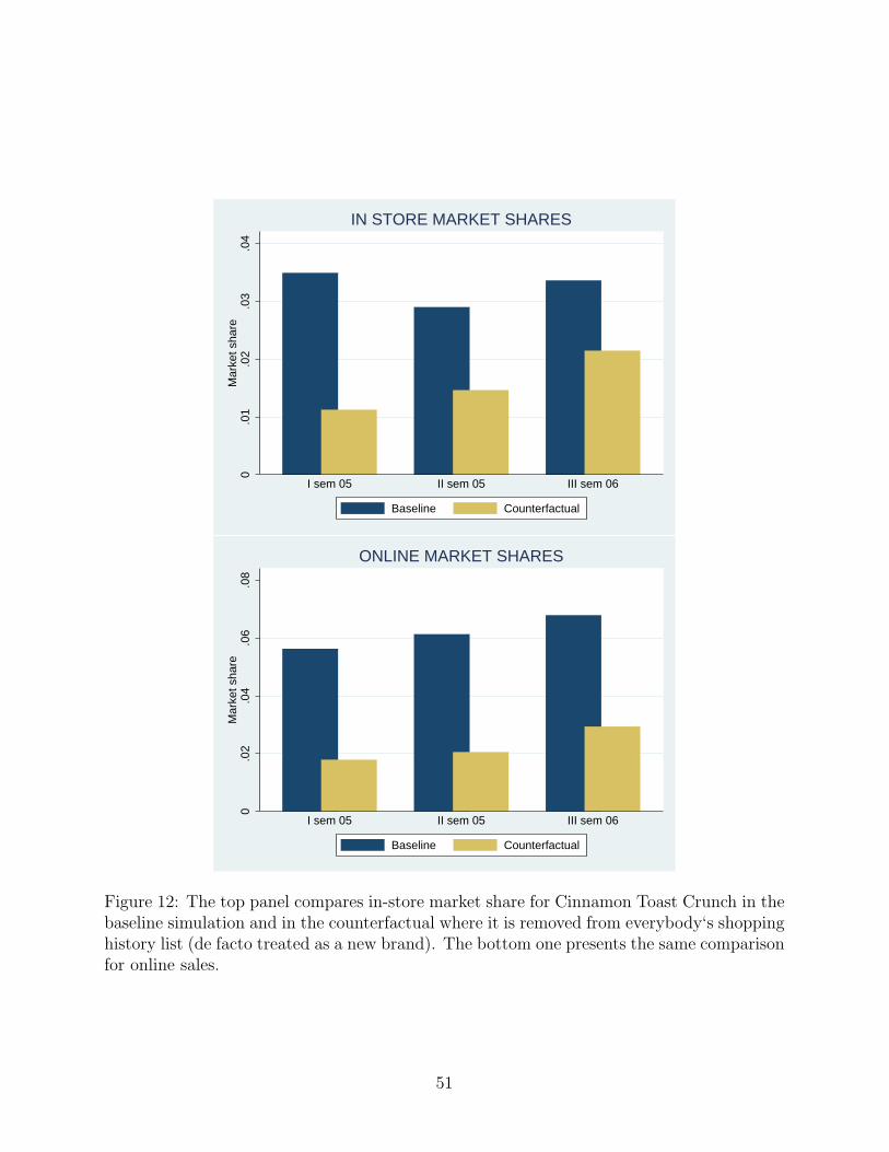
0.0
1.0
2.0
3.0
4M
arke
t sha
re
I sem 05 II sem 05 III sem 06
IN STORE MARKET SHARES
Baseline Counterfactual
0.0
2.0
4.0
6.0
8M
arke
t sha
re
I sem 05 II sem 05 III sem 06
ONLINE MARKET SHARES
Baseline Counterfactual
Figure 12: The top panel compares in-store market share for Cinnamon Toast Crunch in thebaseline simulation and in the counterfactual where it is removed from everybody‘s shoppinghistory list (de facto treated as a new brand). The bottom one presents the same comparisonfor online sales.
51

0.2
.4.6
Sha
re n
ew b
rand
/Sha
re C
inna
mon
Toa
st
I sem 05 II sem 05 III sem 06
Convergence rate
In store Online
Figure 13: The bars represent Cinnamon Toast Crunch’s market share in the counterfactualas a percentage of the same figure in the baseline model.
Figure 14: Screenshot of the shopping history list page, featuring context ads.
52

0.5
11.
52
Sha
re n
ew b
rand
/Sha
re C
inna
mon
Toa
st
I sem 05 II sem 05 III sem 06
Convergence rate
In store Online
Figure 15: The bars represent Cinnamon Toast Crunch’s market share in the counterfactualwith context ads as a percentage of the same figure in the baseline model.
53