
Ship Hull Optimization in Calm Water and Moderate Sea States
102
Ship Hull Optimization in Calm Water and Moderate Sea States Tin Yadanar Tun Master Thesis presented in partial fulfillment of the requirements for the double degree: “Advanced Master in Naval Architecture” conferred by University of Liege "Master of Sciences in Applied Mechanics, specialization in Hydrodynamics, Energetics and Propulsion” conferred by Ecole Centrale de Nantes developed at University of Rostock in the framework of the “EMSHIP” Erasmus Mundus Master Course in “Integrated Advanced Ship Design” Ref. 159652-1-2009-1-BE-ERA MUNDUS-EMMC Supervisor: Dr.Ing. Robert Bronsart, University of Rostock Dipl.-Ing. Eva Binkowski, University of Rostock Internship Supervisor: Dr.-Ing. Stefan Harries, FRIENDSHIP SYSTEMS AG Reviewer: Prof. Florin Pacuraru, University of Galati Rostock, February 2016
Transcript of Ship Hull Optimization in Calm Water and Moderate Sea States

Ship Hull Optimization
in Calm Water and Moderate Sea States
Tin Yadanar Tun
Master Thesis
presented in partial fulfillment
of the requirements for the double degree:
“Advanced Master in Naval Architecture” conferred by University of Liege
"Master of Sciences in Applied Mechanics, specialization in Hydrodynamics,
Energetics and Propulsion” conferred by Ecole Centrale de Nantes
developed at University of Rostock
in the framework of the
“EMSHIP”
Erasmus Mundus Master Course
in “Integrated Advanced Ship Design”
Ref. 159652-1-2009-1-BE-ERA MUNDUS-EMMC
Supervisor: Dr.Ing. Robert Bronsart, University of Rostock
Dipl.-Ing. Eva Binkowski, University of Rostock
Internship Supervisor: Dr.-Ing. Stefan Harries, FRIENDSHIP SYSTEMS AG
Reviewer: Prof. Florin Pacuraru, University of Galati
Rostock, February 2016


Ship Hull Optimization in Calm Water and Moderate Sea States 3
EMSHIP” Erasmus Mundus Master Course, period of study September 2014 – February 2016
ABSTRACT
Optimization is a human trait. Mathematically speaking, it is minimizing (or maximizing) one
or several objectives within a set of constraints. Hull form optimization from a hydrodynamic
performance point of view in calm water and in moderate sea states is an important aspect in
preliminary ship design. The challenge of this work is getting a ship with lowest energy
consumption in calm water and in different sea states by various optimization approaches.
Several optimization approaches were used for a hull form improvement to maximize
seakeeping performance (accelerations based criteria) and minimize the ship resistance at its
given displacement and its service speeds. Different sea-states of operating routes and
different speeds were taken into account for the analysis of seakeeping performance of a
vessel.
An academic container vessel (Duisburg Test Case developed and tested by the University of
Duisburg-Essen) was taken for the study case. The parametric model of the vessel is
developed by modifying the initial geometry with the use of CAESES 4.0. After getting a
parametric model, it was simulated by GL Rankine, potential flow code developed by DNV
GL and validated with experimental results from HSVA. After coupling GL Rankine solver
with CAESES, different optimization approaches were done by using CAESES/Dakota
interface. The optimization was focused on the changes of the forward part of the vessel
(Bulbous bow).
While performing optimization process, not only the main objectives to minimize the energy
consumption of the vessel, also computational effort (how many number of CFD runs needed)
and influence of slightly changes on the operational conditions were taken into account as
major criteria.
As the first approach, the optimal hull form was obtained in calm water condition by different
optimization algorithms and was checked wave added resistance and seakeeping behavior in
moderate sea states. In second approach, optimization process was done by considering calm
water condition and also seakeeping performance in different operation profiles. Finally, the
results of the optimal hull form were compared with original design.


Ship Hull Optimization in Calm Water and Moderate Sea States 5
EMSHIP” Erasmus Mundus Master Course, period of study September 2014 – February 2016
ACKNOWLEDGEMENTS
I would like to say my deepest thanks to those who willingly helped me for this master thesis
and for finishing this master course
Dipl.-Ing. Eva Binkowski and Prof. Dr.-Ing. Robert Bronsart, for making this work possible
and guiding me to the success of the master thesis
Dr.-Ing. Stefan Harries, for his ideas, supervision and orientation in every detail of this
research work
Prof. Philippe Rigo, as coordinator of the EMSHIP for his great effort in organizing and
managing this program and for his constant help and encouragement to finish this great
pleasure and challenging study period in Europe
The FRIENDSHIP SYSTEMS team that made my work possible and pleasant, receiving me
with open arms and answering all my questions
DNV-GL team, especially Mr. Vladimir Shigunov, Mr. Andreas Brehm and Mr. Alexander
Von-Graefe and Jonas Conradin Wagner for their valuable support and advices for technical
problems.
Furthermore, I would like to say thanks to Noufal Paravilayil Najeeb, my colleague for
supporting me and helping me out for everything. Finally, I would like to express my
gratitude towards my family, especially my parents and my friends for supporting me and all
of my teachers who taught me to be in this position.
This thesis was developed in the frame of the European Master Course in “Integrated
Advanced Ship Design” named “EMSHIP” for “European Education in Advanced Ship
Design”, Ref.: 159652-1-2009-1-BE-ERA MUNDUS-EMMC.
Tin Yadanar Tun – Rostock, January, 2015


Ship Hull Optimization in Calm Water and Moderate Sea States 7
“EMSHIP” Erasmus Mundus Master Course, period of study September 2014 – February 2016
TABLE OF CONTENTS
ABSTRACT……………………………….…………………………….…………………… 3
ACKNOWLEDGEMENTS…………….……………………………….…………………… 5
LIST OF FIGURES .................................................................................................................. 10
LIST OF TABLES ................................................................................................................... 13
1. INTRODUCTION ............................................................................................................ 17
1.1. General ....................................................................................................................... 17
1.2. Benefits ...................................................................................................................... 18
1.3. Objectives .................................................................................................................. 18
1.4. Scope of Study ........................................................................................................... 19
1.5. Methods and Procedures ............................................................................................ 19
2. LITERATURE REVIEW .................................................................................................. 21
2.1. Advanced Design Optimization Methods in Dakota.................................................. 23
2.2. Brief Overview of Optimization Methods used in CAESES ..................................... 24
3. CASE STUDY .................................................................................................................. 25
3.1. Main Characteristics of the Vessel ............................................................................ 25
3.2. Operational Profile ..................................................................................................... 26
4. GEOMETRICAL MODELLING ..................................................................................... 28
4.1. Partially-parametric Model ........................................................................................ 30
4.2. Selection of Design Parameters ................................................................................. 33
5. COMPUTATIONAL FLUID DYNAMICS (CFD) METHOD ........................................ 35
5.1. GL Rankine Solver .................................................................................................... 36
5.1.1. Use of GL Rankine Solver ...................................................................................... 36
5.2. Mesh Dependency on Numerical Results .................................................................. 40
5.3. Validation of Numerical Results with Experimental Data ......................................... 42
5.3.1. Description of Experiment ................................................................................. 42
8 Tin Yadanar Tun
Master Thesis developed at University of Rostock, Germany
5.3.2. Comparisons of Result Values for Calm Water Resistance ............................... 43
5.3.3. Comparisons of Result Values for Wave Added Resistance.............................. 45
6. OPTIMIZATION PROCESSES IN CALM WATER CONDITION ............................... 48
6.1. Design of Experiments .............................................................................................. 48
6.2. Single Objective Optimization ................................................................................... 49
6.3. Single Objective Optimization with Weighted Functions ......................................... 53
6.3.1. α = 0.25............................................................................................................... 54
6.3.2. α = 0.50............................................................................................................... 54
6.3.3. α = 0.75............................................................................................................... 55
6.4. Multi-objective Optimization..................................................................................... 56
6.5. Sensitivity Analysis ................................................................................................... 58
6.6. Analysis of Optimal Models at Different Operation Conditions ............................... 59
7. SEAKEEPING ANALYSIS IN MODERATE SEA STATES ......................................... 61
7.1. Added Wave Resistance Due to Head Waves for Initial Model ................................ 61
7.2. Added Wave Resistance Comparison of Optimal Models ......................................... 64
7.3. Direct Optimization of Total Resistance in Waves .................................................... 66
8. RESULTS AND ANALYSIS ........................................................................................... 68
8.1. State of the Art in Optimization for Calm Water Conditions .................................... 68
8.2. Optimal Model Selected from the Optimization in Calm Water ............................... 69
8.3. Optimal Model Selected from the Direct Optimization in Sea States........................ 73
8.3.1. Analysis of the Optimal Models for Different Wave Heading Angles .............. 74
9. SUMMARY ...................................................................................................................... 79
10. CONCLUSION AND RECOMMENDATIONS .......................................................... 81
10.1. Conclusion ................................................................................................................... 81
10.2. Recommendations .................................................................................................. 82
REFERENCES ......................................................................................................................... 83
APPENDIX .............................................................................................................................. 85

Ship Hull Optimization in Calm Water and Moderate Sea States 9
“EMSHIP” Erasmus Mundus Master Course, period of study September 2014 – February 2016
A1. Study on Each Design Parameters ................................................................................. 85
A2. Set-up Input XML File for GL Rankine Solver ............................................................. 90
A2.1. Sample XML file for Steady Flow Computation .................................................... 90
A2.2. Sample XML file for Seakeeping Computation ...................................................... 92
A3. Distribution of Design Variables by SOBOL in Design Space ...................................... 94
A4. Standard Template for Surrogate Based Global Optimization (CAESES) .................. 100
A5. MATLAB Code for Calculating the Added Wave Resistance ..................................... 101

10 Tin Yadanar Tun
Master Thesis developed at University of Rostock, Germany
LIST OF FIGURES
Figure - 1: Phases of Product Development [1] ....................................................................... 18
Figure- 2: Flow Chart showing Methods and Procedures ........................................................ 20
Figure - 3: General Flowchart of Genetic Algorithm [8] ......................................................... 23
Figure- 4: Original Hull Form Design ...................................................................................... 26
Figure- 5: Operation Scenarios Considering Actual Sea State Information ............................ 26
Figure- 6: Operation Scenarios without Considering Actual Sea State Information ............... 27
Figure- 7: Process flow of parametric model in optimization ................................................. 28
Figure- 8: Partially-parametric model for a downward vertical shift (left column), the baseline
(middle) and an upward vertical shift (right column) applied to both B-spline surface patches
and tri-meshes [1] ..................................................................................................................... 30
Figure- 9: Base Model Geometry in Tri-mesh STL format ..................................................... 31
Figure- 10: Feature definition curve generation and surface generation for surface delta shift
.................................................................................................................................................. 31
Figure- 11: Initial mesh (Blue) and new sections after surface delta shift ............................... 32
Figure- 12: Partial parametric model. Diver view created at CAESES ................................... 32
Figure- 13: Varying of bulbous bow shape by controlling design parameters in transverse
direction [Initial mesh (left) and modified mesh (right)] .......................................................... 34
Figure- 14: Varying of bulbous bow shape by controlling design parameters in longitudinal
direction .................................................................................................................................... 34
Figure- 15: CFD methods with their accuracy and CPU time (Ferrant (2013) [16]) ............... 35
Figure- 16: Typical STL triangular grid of a ship half ............................................................. 37
Figure- 17: Typical panels generated by GL Rankine on a STL surface ................................. 38
Figure- 18: Automatically created structured free surface mesh in GL Rankine depending on
speed ......................................................................................................................................... 38
Figure- 19: Mesh Dependency for different Froude Numbers ................................................. 41
Figure- 20: Comparison of Wave Resistance Coefficients (Cw) ............................................. 44
Figure- 21: Comparison of resistance in calm water condition ............................................... 45
Figure- 22: Comparison of added wave resistance coefficient (T=14.5m, Vs = 16 knots) ..... 47
Figure- 23: Exploration of Design Space [23] ......................................................................... 48
Figure- 24: Single objective optimization at 15.5 knots .......................................................... 49
Figure- 25: Wave height comparison between Base model and optimal model ...................... 50
Figure- 26: Wave profile comparison between base and optimal model (V=15.5 knots) ....... 50

Ship Hull Optimization in Calm Water and Moderate Sea States 11
“EMSHIP” Erasmus Mundus Master Course, period of study September 2014 – February 2016
Figure- 27: Base model and optimal model comparison (V =15.5 knots) ............................... 51
Figure- 28: Single objective optimization at 18 knots ............................................................. 51
Figure- 29: Wave cut comparison between base and optimal model (V=18 knots) ................ 52
Figure- 30: Base model and optimal model comparison (V =18 knots) .................................. 52
Figure- 31: Comparison of Single objective optimization for 15.5 knots and 18 knots .......... 53
Figure- 32: Single objective optimization with α= 0.25 .......................................................... 54
Figure- 33: Single objective optimization with α= 0.50 .......................................................... 54
Figure- 34: Single objective optimization with α= 0.75 .......................................................... 55
Figure- 35: Convergence study of surrogate based global optimization .................................. 56
Figure- 36: Multi-Objective Optimization (Dakota- SBGO) ................................................... 57
Figure- 37: Multi-Objective Optimization (Dakota- SBGO) zoomed in design of interest ..... 57
Figure- 38: Sensitivity analysis of draft variation for selected designs at V1 = 15.5 knots ..... 58
Figure- 39: Sensitivity analysis of draft variation for selected designs at V2 = 18 knots ........ 59
Figure- 40: Comparison of Difference in RT (%) related to base model at different operation
conditions ................................................................................................................................. 60
Figure- 41: Scatter Diagram of wave data at T= 15m, V=18 knots ......................................... 61
Figure- 42: Added wave resistance due to head waves for the initial base model ................... 62
Figure- 43: Added wave resistance due to head waves for the initial base model ................... 63
Figure- 44: Added wave resistance due to head waves for initial base model for area of
interest only .............................................................................................................................. 63
Figure- 45: Added wave resistance due to head waves for initial base model for area of
interest only .............................................................................................................................. 64
Figure- 46: DoEs by SOBOL and Optimal Model for V1 = 15.5 knots, T1=14.5m ............... 67
Figure- 47: DoEs by SOBOL and Optimal Model for V2 = 18 knots, T2=15m ..................... 67
Figure- 48: Comparison of Diff: % in RT for different operation conditions .......................... 69
Figure- 49: Wave pattern of the optimal and base hull form (V=15.5knots, T=14.5m) .......... 70
Figure- 50: Wave Profile for Base and Optimum model (V=15.5knots, T=14.5m) ................ 70
Figure- 51: Wave Cut at Y/LPP=0.2 for Base and Optimum model (V=15.5knots, T=14.5m)
.................................................................................................................................................. 71
Figure- 52: Base model and final optimal model comparison (V =15.5 knots, T= 14.5m) ..... 71
Figure- 53: Total resistance of base model and optimal model at whole range of operational
speeds at T=14.5m [In the secondary axis the relative difference in percentage is presented] 72
Figure- 54: Total resistance of base model and optimal model at whole range of operational
speeds at T=14.0m.................................................................................................................... 72

12 Tin Yadanar Tun
Master Thesis developed at University of Rostock, Germany
Figure- 55: Total resistance of base model and optimal model at whole range of operational
speeds at T=15.0m.................................................................................................................... 73
Figure- 56: Added wave resistance/ Rt (Calm water) (%) for head waves .............................. 75
Figure- 57: Added wave resistance/ Rt (Calm water) (%) in seaway 30 deg off bow ............. 75
Figure- 58: Added wave resistance/ Rt (Calm water) (%) in seaway 60 deg off bow ............. 76
Figure- 59: Added wave resistance at V1=15.5knots, T1=14.5m and Hs=1.25m ................... 76
Figure- 60: Added wave resistance at V2=18knots, T2=15m and Hs=1.75m ......................... 77
Figure- 61: Comparison of Geometry of Bulbous Bow in Longitudinal View ....................... 77
Figure- 62: Comparison of Geometry of Bulbous Bow in Transverse View ........................... 78
Figure- A1- 1: Influence of bulb length variable on ship total resistance ................................ 85
Figure- A1- 2: Influence of bulb width variable on ship total resistance ................................. 86
Figure- A1- 3: Influence of bulb tip elevation variable on ship total resistance ...................... 87
Figure- A1- 4: Influence of WL entrance angle variable on ship total resistance ................... 88
Figure- A1- 5: Influence of Bulb top tangent at FP variable on ship total resistance .............. 89
Figure-A3- 1: Distribution of the values of parameter “dx-bulb” ............................................ 94
Figure-A3- 2: Distribution of the values of parameter “dy-bulb” ............................................ 94
Figure-A3- 3: Distribution of the values of parameter “dz-bulb” ............................................ 95
Figure-A3- 4: Distribution of the values of parameter “bulbTangent_FP” ............................. 95
Figure-A3- 5: Distribution of the values of parameter “EntranceAngle” ................................ 96
Figure-A3- 6: Distribution of the values of parameter “Difference in RTV1 from BM” ........ 96
Figure-A3- 7: Distribution of the values of parameter “Difference in RTV2 from BM” ........ 97
Figure-A3- 8: Distribution of the values of parameter “RTV1” .............................................. 97
Figure-A3- 9: Distribution of the values of parameter “RTV2” .............................................. 98
Figure-A3- 10: Distribution of total resistance with weight coefficient= 0.25 ........................ 98
Figure-A3- 11: Distribution of total resistance with weight coefficient= 0.50 ........................ 99
Figure-A3- 12: Distribution of total resistance with weight coefficient= 0.75 ........................ 99

Ship Hull Optimization in Calm Water and Moderate Sea States 13
“EMSHIP” Erasmus Mundus Master Course, period of study September 2014 – February 2016
LIST OF TABLES
Table - 1: Main Dimensions of DTC in Design Loading Condition ........................................ 25
Table - 2: Variation of grid parameters .................................................................................... 40
Table - 3: Number of Panels for Different Froude Numbers ................................................... 40
Table - 4: Wave resistance coefficients for different mesh ...................................................... 41
Table - 5: Particulars of model scale and full scale of DTC container vessel .......................... 42
Table - 6: Results of resistance model tests ............................................................................. 43
Table - 7: Results of GL Rankine Simulations ........................................................................ 44
Table - 8: DTC added resistance coefficient results ................................................................ 46
Table - 9: Result summary for single objective optimization processes .................................. 55
Table - 10: Total resistance for selected optimal models at different operation conditions .... 60
Table - 11: Wave scenario data for two operation conditions .................................................. 64
Table - 12: Comparison of total resistance due to waves of optimum models at two speeds .. 65
Table - 13: Number of CFD runs and Total resistance in waves related to base model % ...... 68
Table - 14: Geometry trend of the optimized bulbous bow ..................................................... 69
Table - 15: CFD runs and Total resistance in waves related to base model % in sea states .... 73
Table - 16: Geometry trend of the optimized bulbous bow ( optimization in sea states) ........ 74
Table - 17: Performance Summary of the final optimal models for two operation conditions 80

14 Tin Yadanar Tun
Master Thesis developed at University of Rostock, Germany

Ship Hull Optimization in Calm Water and Moderate Sea States 15
“EMSHIP” Erasmus Mundus Master Course, period of study September 2014 – February 2016
DECLARATION OF AUTHORSHIP
I declare that this thesis and the work presented in it are my own and have been generated by
me as the result of my own original research.
Where I have consulted the published work of others, this is always clearly attributed.
Where I have quoted from the work of others, the source is always given. With the exception
of such quotations, this thesis is entirely my own work.
I have acknowledged all main sources of help.
Where the thesis is based on work done by myself jointly with others, I have made clear
exactly what was done by others and what I have contributed myself.
This thesis contains no material that has been submitted previously, in whole or in part, for
the award of any other academic degree or diploma.
I cede copyright of the thesis in favor of the University of Rostock.
Date: Signature:

16 Tin Yadanar Tun
Master Thesis developed at University of Rostock, Germany
Ship Hull Optimization in Calm Water and Moderate Sea States 17
“EMSHIP” Erasmus Mundus Master Course, period of study September 2014 – February 2016
1. INTRODUCTION 1.1. General
The hydrodynamic performance of a hull form in calm water and in moderate sea state is a
major aspect for a naval architect in preliminary design stage. In the past, ships were
designed based on the performance in calm water condition without considering the sea state
of actual operation profiles and there are many attempts to optimize the calm water
resistance of the vessel by varying form parameters. On the other hand, both of the
global and local form parameters of a vessel influence its calm water behavior as well as its
seakeeping performance depends primarily on global hull form parameters. Therefore, in
recent years, the optimization of vessel both in calm water and in its seaways becomes
more important for the reliable prediction of the power requirement. In the optimization
process, the different algorithm is linked to the computational method to obtain an
optimum hull form by several geometrical constraints such as internal fitting, displacement
and stability.
There are different kinds of approaches to study hydrodynamic performance which are (a) the
empirical approach that is in the form of constants, formulae and curves developed from the
parent ship or similar shapes, (b) the experimental approach that is the testing of a scaled model
of original hull form and analyzing the performances, expanding to full scale results and (c)
the numerical approach that has become increasingly important for ship resistance and
powering. Therefore, ship optimization based on CFD simulation becomes the major factor of
developing new optimal ship hull forms by minimizing ship resistance. Reducing the
resistance leads to less consumable power, less emissions and noises.
The optimization process is fully automated requiring no user interaction. In this thesis, the
steady wave system of a ship moving through calm water is approximated by means of CFD
(Computational Fluid Dynamics) simulation applying nonlinear free surface Rankine panel
method of GL Rankine solver, which is in-house potential flow solver developed by DNV GL.
The modelling of the geometry of the initial design, the coupling of the CFD solver and
performing the optimization process to minimize the wave-making resistance were done by the
use of CAESES developed by FRIENDSHIP SYSTEMS.

18 Tin Yadanar Tun
Master Thesis developed at University of Rostock, Germany
1.2. Benefits
Ship hull form optimization offers several benefits in the way of:
Better understanding of the design task (and the design space),
Creating design with superior performance (and better trade-offs),
Allowing shorter time-to-market (and faster response to market changes),
Reducing risk (and building confidence),
Saving costs (and avoiding expensive late changes).
Hull form optimization is conducted both for investigating new ideas and possibilities at the
initial design stage and for fine-tuning of a given design at a later stage when only small changes
are still acceptable, sees Figure - 1.
Figure - 1: Phases of Product Development [1]
1.3. Objectives
The main objective of this thesis is to study about the various approaches for the optimization
of fore body (Bulbous Bow) of hull form for a container vessel based on the given
technical specifications. The optimization process will be focused on minimizing the
wave-making resistance of the vessel in calm water condition and added resistance in its
seaway conditions. Furthermore, the coupling of newly developed in-house GL Rankine
solver with CAESES, to check the resistances in both steady flow and seaway, as well as the
seakeeping performances considering different scenarios of operating routes and different
speeds, has to be done.

Ship Hull Optimization in Calm Water and Moderate Sea States 19
“EMSHIP” Erasmus Mundus Master Course, period of study September 2014 – February 2016
1.4. Scope of Study
In this thesis, the hull form for the specific vessel will be optimized with fully-automated
process, but it is allowed to operate manually as well. The fore body of hull form is modelled
as partial parametric model in CAESES and it is simulated with GL Rankine potential flow
solver for obtaining the resultant resistances in calm water and in seaways, followed by
validating the results from experiments which are performed in model basin at HSVA.
The optimization process will be done with CAESES/ Dakota Interface to get the optimized
hull form that can be checked later for seakeeping behaviors with moderate sea states. The set-
up optimization process permits to get the best hull form which is not only the resistance in
calm water but also for added resistance in seaways as well.
1.5. Methods and Procedures
The original hull form trimesh of a DTC (Duisburg Test Case) container vessel, given by
Duisburg University in STL format is modified in CAESES using the design parameters which
control the shape of bulbous bow of the vessel. After getting a partially parametric model,
the setup of GL Rankine solver is developed in order to get the simulation results such as
calm water resistance, added wave resistance and 6 DOF motions. The results obtained
from CFD solver are verified with the experimental results performed by HSVA towing
tanks. After that, the CFD solver is coupled with CAESES to perform different
optimization processes for different scenarios considering actual seaways, which cover
approximately 37% of operation profiles of similar container vessels calculated by University
of Rostock.
In addition to finding the optimal hull form with the minimum calm water resistance and
checking seakeeping behaviors, the direct optimization of calm water resistance together with
added resistance in waves will also be done. Optimization will be done especially on the fore
body of the hull, (e.g. bulbous bow) because GL Rankine solver utilizes the potential flow code
which is mainly effective for fore body flow of the ship and less effective for viscous flow
occurred at the aft body.
The flow chart showing the step by step procedure of the entire work scope can be seen in
Figure - 2.

20 Tin Yadanar Tun
Master Thesis developed at University of Rostock, Germany
Figure- 2: Flow Chart showing Methods and Procedures
Partial Parametric Model of Given Geometry (Bulbous Bow)
Test Simulation with GL Rankine and Mesh Convergence Study
Validation of Results with HSVA Experimental Data
Optimization in Calm Water
Condition and computing
seakeeping performance for
selected optimal design
Direct optimization for both
calm water resistance and added
resistance in moderate sea state
Different Optimization Approaches
Single Objective Function
Single Objective with Weighted Functions
Multi-objective function with Genetic Algorithm
Selection of Optimal Design and Comparison with Initial Model

Ship Hull Optimization in Calm Water and Moderate Sea States 21
“EMSHIP” Erasmus Mundus Master Course, period of study September 2014 – February 2016
2. LITERATURE REVIEW
This thesis includes different optimization processes for the improvement of ship
hydrodynamic performance such as calm water resistance, added resistance in waves for
different operation profiles at different speeds and its seakeeping performances. Before
starting optimization process of ship hull form, the author has done numerous
engineering studies related to parametric modelling of ship hull form, coupling of GL
Rankine potential flow solver with CAESES, designing the sea states of vessel’s operation
routes for its seakeeping performances, various optimization algorithms and so on. In this
literature review, some aspects of optimization process of different hull shapes for resistance
and seakeeping performance in calm water and in moderate sea states are presented for the
better understanding of the problem. Prediction of Ship performances in calm and rough water
is one of the most important concerns for naval architects, already at the earliest design stage.
From this point of view, seakeeping performance is one of the most important performances
in the ship hull form optimization (Bagheri, Ghassemi and Dehghanian, 2014 [2]).
Zhang et al (2008) [3] wrote a paper about “Parametric Approach to Design of Hull Forms”
in Eslevier Journal. This paper covers the parametric modelling of the hull form with the
use of form parameters and the longitudinal function curves and combining the parametric
approach to CFD method for optimization. After several principle dimensions have been
fixed as a result of economic and/or hydrodynamic optimizations, a subsequent improvement
of the hydrodynamic performance is usually carried out to refine the design. Parameters
typically used for the manipulation of wave resistance are related to the shape of the bulbous
bow. (Abt et al, 2001[4]).
After designing parametric model of a vessel, numerical analysis of hydrodynamic performance
has to be done by the use of CFD (computational fluid dynamics) solvers. CFD methods
provide total resistance, i.e., calm water resistance and added resistance in waves. But CFD
methods require too much computer resources to study the influence of various parameters
on added resistance, potential flow methods are applied predominantly. (Heinrich et al, 2012
[5]). Heimann (2005) [6] wrote a PhD thesis about “CFD based Optimization of the wave-
making characteristics of ship hulls” that covers a hull form optimization approach with
CFD based evaluation of the nonlinear ship wave pattern, on realization of the cause and
effect relation of hull variations and their impact on wave formation, which is accessed
by a perturbation approach, and on wave cut analysis (WCA).

22 Tin Yadanar Tun
Master Thesis developed at University of Rostock, Germany
A paper about “Hull-form optimization in calm and rough water” presents a formal
methodology for the hull form optimization in calm and rough water using wash waves and
selected dynamic responses, respectively. A major concern of any optimization procedure is
to associate the set of hull form parameters identifying the variants to a faired hull form.
Parametric models offer the only way to establish this relation and to ensure that at each
stage of the optimization a feasible model is produced. Then, state-of-the-art algorithms
can evaluate its hydrodynamic performance both in calm and rough water by the use of
Rankine-source panel method and strip theories (Grigoropoulos and Chalkias, 2009 [7]).
Genetic algorithm is inspired by the evolution theory (Darwin’s theory of biological evolution)
by means of a process that is known as the natural selection and the "survival of the fittest"
principle. The common idea behind this technique is similar to other evolutionary algorithms:
consider a population of individuals; the environmental pressure causes natural selection which
leads to an increase in the fitness of the population. It is easy to see such a process as
optimization.
Consider an evaluation function to be minimized (the lower, the better). A set of candidate
solutions can be randomly generated and the objective function can be used as a measure of
how individuals have performed in the problem domain (an abstract fitness measure).
According to this fitness, some of the better solutions are selected to seed the next generation
by applying recombination and/or mutation operators to them. The recombination (also called
crossover) operator is used to generate new candidate solutions (offspring) from existing ones
by taking two or more selected candidates (parents) from the population pool and by exchanging
some of their parts to form one or more offspring. The mutation operator is used to generate
one offspring from one parent by changing some parts of the candidate solution. The application
of the recombination and mutation operators causes a set of new candidates (the offspring) to
compete based on their fitness with the old candidates (the parents) for a place in the next
generation.
This procedure can be iterated until a solution with sufficient quality (fitness) is found or a
previously set computational time limit is reached. In other words, the end conditions must be
satisfied. The composed application of selection and variation operators (recombination and
mutation) improves fitness values in the consecutive population. A general flowchart of
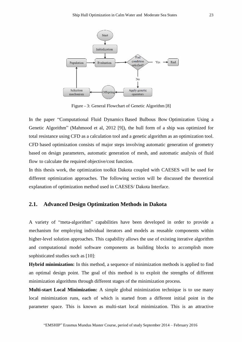
genetic algorithm is shown in Figure - 3 (Bagheri et al, 2014[8]).
Ship Hull Optimization in Calm Water and Moderate Sea States 23
“EMSHIP” Erasmus Mundus Master Course, period of study September 2014 – February 2016
Figure - 3: General Flowchart of Genetic Algorithm [8]
In the paper “Computational Fluid Dynamics Based Bulbous Bow Optimization Using a
Genetic Algorithm” (Mahmood et al, 2012 [9]), the hull form of a ship was optimized for
total resistance using CFD as a calculation tool and a genetic algorithm as an optimization tool.
CFD based optimization consists of major steps involving automatic generation of geometry
based on design parameters, automatic generation of mesh, and automatic analysis of fluid
flow to calculate the required objective/cost function.
In this thesis work, the optimization toolkit Dakota coupled with CAESES will be used for
different optimization approaches. The following section will be discussed the theoretical
explanation of optimization method used in CAESES/ Dakota Interface.
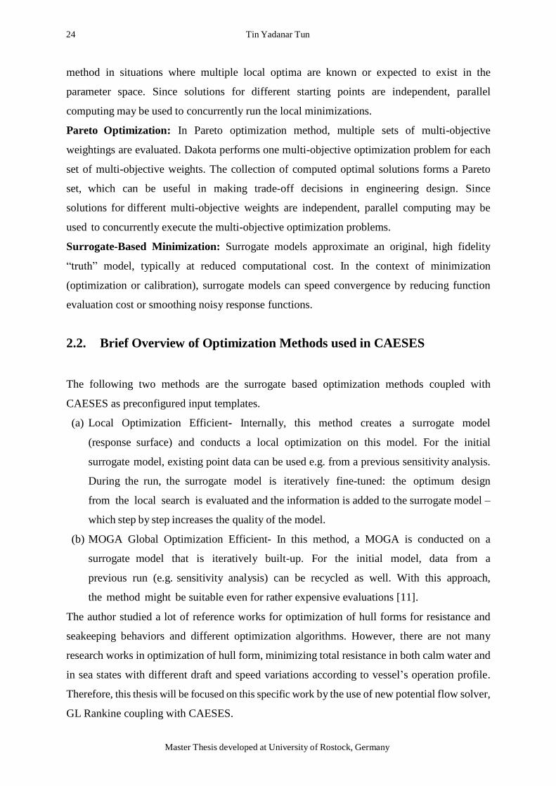
2.1. Advanced Design Optimization Methods in Dakota
A variety of “meta-algorithm” capabilities have been developed in order to provide a
mechanism for employing individual iterators and models as reusable components within
higher-level solution approaches. This capability allows the use of existing iterative algorithm
and computational model software components as building blocks to accomplish more
sophisticated studies such as [10]:
Hybrid minimization: In this method, a sequence of minimization methods is applied to find
an optimal design point. The goal of this method is to exploit the strengths of different
minimization algorithms through different stages of the minimization process.
Multi-start Local Minimization: A simple global minimization technique is to use many
local minimization runs, each of which is started from a different initial point in the
parameter space. This is known as multi-start local minimization. This is an attractive
24 Tin Yadanar Tun
Master Thesis developed at University of Rostock, Germany
method in situations where multiple local optima are known or expected to exist in the
parameter space. Since solutions for different starting points are independent, parallel
computing may be used to concurrently run the local minimizations.
Pareto Optimization: In Pareto optimization method, multiple sets of multi-objective
weightings are evaluated. Dakota performs one multi-objective optimization problem for each
set of multi-objective weights. The collection of computed optimal solutions forms a Pareto
set, which can be useful in making trade-off decisions in engineering design. Since
solutions for different multi-objective weights are independent, parallel computing may be
used to concurrently execute the multi-objective optimization problems.
Surrogate-Based Minimization: Surrogate models approximate an original, high fidelity
“truth” model, typically at reduced computational cost. In the context of minimization
(optimization or calibration), surrogate models can speed convergence by reducing function
evaluation cost or smoothing noisy response functions.
2.2. Brief Overview of Optimization Methods used in CAESES
The following two methods are the surrogate based optimization methods coupled with
CAESES as preconfigured input templates.
(a) Local Optimization Efficient- Internally, this method creates a surrogate model
(response surface) and conducts a local optimization on this model. For the initial
surrogate model, existing point data can be used e.g. from a previous sensitivity analysis.
During the run, the surrogate model is iteratively fine-tuned: the optimum design
from the local search is evaluated and the information is added to the surrogate model –
which step by step increases the quality of the model.
(b) MOGA Global Optimization Efficient- In this method, a MOGA is conducted on a
surrogate model that is iteratively built-up. For the initial model, data from a
previous run (e.g. sensitivity analysis) can be recycled as well. With this approach,
the method might be suitable even for rather expensive evaluations [11].
The author studied a lot of reference works for optimization of hull forms for resistance and
seakeeping behaviors and different optimization algorithms. However, there are not many
research works in optimization of hull form, minimizing total resistance in both calm water and
in sea states with different draft and speed variations according to vessel’s operation profile.
Therefore, this thesis will be focused on this specific work by the use of new potential flow solver,
GL Rankine coupling with CAESES.

Ship Hull Optimization in Calm Water and Moderate Sea States 25
“EMSHIP” Erasmus Mundus Master Course, period of study September 2014 – February 2016
3. CASE STUDY
Hydrodynamic optimization of ships not only targets energy efficiency but also the performance
of ships in moderate and heavy sea states. The research and development project, called PerSee
which stands for “Performance von Schiffen im Seegang” (performance of ships in sea-states),
aims at establishing new processes for the optimization of ships in moderate seas, considering
the effects of waves on both hull forms and propellers, and at identifying safety requirements
for ships in heavy seas. Operational scenarios as well as minimum speed and power
requirements are considered. The engineers from Friendship Systems become a part of the
project called PerSee, which studies the optimization of ships in sea states. Within the project,
Friendship Systems further strengthens its CAE platform CAESES. Main R&D targets are
further ease in setting up complex processes that involve several simulation tools and improved
usability in creating and understanding complex parametric models [12]. In this PerSee project,
among different coordinated work packages, Friendship Systems has to perform parametrical
optimization of the hull shape under operating conditions in seaways [13]. In this thesis work,
the new DTC (Duisburg Test Case) container vessel is needed to optimize for calm water
resistance and motion performances in moderate seaways by applying the in-house potential
flow solver called GL Rankine in CAESES.
3.1. Main Characteristics of the Vessel
The study relies on a DTC container vessel. Duisburg Test Case (DTC) is a hull design of a
modern 14000 TEU post-panamax container carrier, developed at the University of Duisburg-
Essen, Duisburg, Germany. Table-1 shows main particulars in the design loading condition and
Figure -4 shows the original hull form design [14].
Table - 1: Main Dimensions of DTC in Design Loading Condition
Length Between Perpendiculars Lpp [m] 355.0
Waterline Breadth Bwl [m] 51.0
Design Draft Amidships TDm [m] 14.5
Moulded Depth D [m] 32.0
Block Coefficient CB [-] 0.661
Volume Displacement V [m3] 173467.0
wetted surface under rest waterline without appendages SW [m2] 22032.0

26 Tin Yadanar Tun
Master Thesis developed at University of Rostock, Germany
Figure- 4: Original Hull Form Design
3.2. Operational Profile
The robustness of the hull form is checked according to the operational profile, the observed
variation on draft and speed of the ship. As this container vessel has not been built and it is
only in preliminary design state, the operating information of this vessel is statistically derived
from similar vessels in operation.
The wave scenario that the vessel has to deal with are resulted for specific wave height (H1/3)
and are chosen for three operating conditions, covering 50% of the total operating time by the
vessel as mentioned in Figure-5. The weighted values wtotal is represented in the percentage of the
respective operating conditions with respect to total operating time of the vessel.
Figure- 5: Operation Scenarios Considering Actual Sea State Information

Ship Hull Optimization in Calm Water and Moderate Sea States 27
“EMSHIP” Erasmus Mundus Master Course, period of study September 2014 – February 2016
Figure-6 shows the operation scenarios without consideration of any sea state information
(fast speed / draft combination) covering 46% of the total operating time.
Figure- 6: Operation Scenarios without Considering Actual Sea State Information
Since the main objective of this thesis is to get optimal hull for both calm water and actual sea
state condition, the operation scenario by considering sea state was chosen as following.
Operation Condition 1: V=15.5 knots and T= 14.5m
Operation Condition 2: V=18.0 knots and T= 15.0m
Operation Condition 3: V=10.0 knots and T= 13.0m
Nevertheless, V1 = 15.5 knots and V2=18.0 knots are to be used as the main condition for
optimization process at the design draft of T=14.5m. Different optimization approaches will
be done with the above two speeds and afterwards, the robustness checking according to the
draft variation will be performed. For each optimal hull model, the comparison of its
hydrodynamic performance will be done for different operation conditions.
28 Tin Yadanar Tun
Master Thesis developed at University of Rostock, Germany
4. GEOMETRICAL MODELLING
The optimization of a ship’s resistance (to be minimized) is concerned with the geometric
entities that describe the shape variation. Therefore, geometrical modelling plays an important
role and many optimization processes follow the repetitive sequence of shape generation,
analysis and performance assessment. Since CFD analysis constitutes time-consuming part of
an optimization process, the outcome depends on the quality of geometric modelling. For
complex shapes, a high level of sophistication is needed to reduce the number of parameters
that control the geometry.
In the context of optimization of the vessel’s hydrodynamic performance, a conventional non-
parametric approach has numerous disadvantages because the geometry is typically generated
from low level entities. The challenge lies in establishing a functional description of the
modelling problem that corsets undesirable shapes without impairing the necessary freedom
of variation. An excellent approach that allows this is parametric modelling [15].
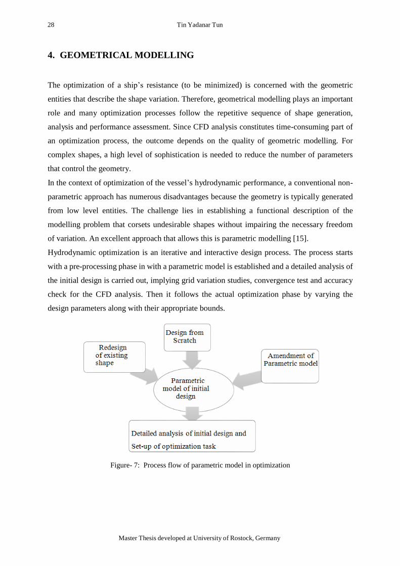
Hydrodynamic optimization is an iterative and interactive design process. The process starts
with a pre-processing phase in with a parametric model is established and a detailed analysis of
the initial design is carried out, implying grid variation studies, convergence test and accuracy
check for the CFD analysis. Then it follows the actual optimization phase by varying the
design parameters along with their appropriate bounds.
Figure- 7: Process flow of parametric model in optimization

Ship Hull Optimization in Calm Water and Moderate Sea States 29
“EMSHIP” Erasmus Mundus Master Course, period of study September 2014 – February 2016
For shape optimization using CFD, special parametric models are needed, so-called engineering
models, which describe the product with as few significant parameters as possible,
sometimes deliberately leaving out characteristics of lesser importance. These models address
the concept and the preliminary design phases, focusing on simulation-ready CAD, and are
realized within upfront CAD systems. Two major traits of upfront CAD are distinguished:
Fully-parametric modelling and partially-parametric modelling [1].
In fully-parametric modelling, the entire shape is defined by means of parameters. Some
parameters may be at a high level like the length, width and height of a vessel. Other parameters
may determine details like an entrance angle at a particular location. Typically, many
parameters are set relative to or as combinations of other parameters. Any shape is realized from
scratch and variants are brought about by simply changing the values of one or several
parameters. For optimization, fully-parametric modeling is very powerful since it enables both
large changes in the early design phase and small adjustments when fine-tuning at a later point
in time.
In partially-parametric modelling, only the changes to an existing shape are defined by
parameters while the baseline (initial design model) is taken as input. Partially-parametric
models are usually quick and fairly easy to set up. When compared to fully-parametric models
they typically contain less knowledge (intelligence) about the product. In general, it is more
difficult to excite large modifications. After all, the new shapes are derived from the baseline
and, thus, cannot look totally different. Still, they are well suited for fine-tuning without much
overhead. Prominent representatives of partially-parametric modelling are morphing; free-
form deformation and shift transformation (e.g. shifts in coordinate direction, radial shifts).
Shift transformations typically change any point in space by adding a certain displacement
depending on the point’s initial position. It can be applied to both continuous data (e.g. surface
patches) and discrete data (e.g. points, offsets, tri-meshes as used for data exchange via STL).
Figur-8 gives an example realized in CAESES, showing a vertical shift of a container
ship’s bulbous bow.

30 Tin Yadanar Tun
Master Thesis developed at University of Rostock, Germany
Figure- 8: Partially-parametric model for a downward vertical shift (left column), the baseline
(middle) and an upward vertical shift (right column) applied to both B-spline surface patches and tri-
meshes [1]
4.1. Partially-parametric Model
Since the idea of this research work is to minimize the resistance by refitting a bulbous bow,
the parametric model for this task was focused on the bulbous bow region only and maintained
the section shape at the forward perpendicular. Instead of implementing a completely new
geometry for this study, a partial parametric model was implemented. Such model relies on
a baseline geometry definition which is modified by means of various shift and scaling
functions. In order to optimize the vessel, some parameters are selected to control the
changes on the selected area of the geometry. The selection of parameters was based on an
extended study of the influence of each variable regarding it optimization improvement i.e.
the “capability” of each parameter on reducing the wave resistance and total resistance of the
vessel.
First, the initial geometry of the DTC container vessel is imported to CAESES as a tri-mesh as
used for data exchange via STL format [see in Figure-9]. The surface delta shift method was
used to get partial parametric model in order to get different bulb shape by changing selected
design parameters.

Ship Hull Optimization in Calm Water and Moderate Sea States 31
“EMSHIP” Erasmus Mundus Master Course, period of study September 2014 – February 2016
Figure- 9: Base Model Geometry in Tri-mesh STL format
First the principal parameters such as length overall, length between perpendiculars, beam, deck
height and XFwdBase (the forward end position of Flat of Bottom), etc., were set-up. Then, the
parametric bulb modification parameters were defined for the variation of shape.
Firstly, the feature definition curves for variation of bulb in x, y and z directions. Then, the
surfaces based on those feature definition curves are generated in order to perform surface delta
shift to baseline (initial design). The detail information about the usage of surface delta shift in
order to get parametric model was omitted in this thesis.
The following figures 10 and 11 show the step by step procedure in order to get the partial
parametric model for the bulbous bow shape variation.
Figure- 10: Feature definition curve generation and surface generation for surface delta shift

32 Tin Yadanar Tun
Master Thesis developed at University of Rostock, Germany
Figure- 11: Initial mesh (Blue) and new sections after surface delta shift
Figure- 12: Partial parametric model. Diver view created at CAESES

Ship Hull Optimization in Calm Water and Moderate Sea States 33
“EMSHIP” Erasmus Mundus Master Course, period of study September 2014 – February 2016
4.2. Selection of Design Parameters
After generating the partial parametric model, there are 14 parameters controlling the
bulbous bow shape variation in total. Some parameters have large effect on the changing of
the bulb geometry and some only have little influence. Furthermore, the principal parameters
that define the main dimension of the hull form cannot be changed.
The number of design parameters should be as minimum as possible in order to be more
efficient in the optimization process. The large number of design variables can lead to the very
large amount of designs while combining all parameters. The design of experiments (DoE)
study provides information to classify the design variables in order of influence to the resistance
reduction. Therefore, it is necessary to define the important design variable parameters in order
to save computational time and to be user-friendly for those who do not know the detail of the
parametric model.
(a) Dx Bulb – A longitudinal shift of the bulb sections to allow elongation or shortening of
the bulbous bow. The variation range for the longitudinal position of bulb tip from base
design is from -2 m to +2 m.
(b) Dy Bulb – In order to allow for changes in width of the bulb, a scaling function has
been used which gradually decreases when approaching the forward perpendicular to
match the unaltered hull shape. The variation range for the half width of the bulb from base
design is from -1 m to +2 m.
(c) Dz Bulb– a vertical shift of the bulb sections to allow the bulbous bow tip to be lowered
or raised with respect to the baseline bulb. As the bulb geometry at the FP could not be
changed, this shift was fading out when approaching the FP. The variation range of bulb tip
elevation from the original base design is from -1.5m to 1.5m.
(d) Bulb top tangent at FP– It is the inclination of the after part of the bulb that connects it
to the hull. It ranges from -5 degree to 11 degree.
(e) Entrance Angle DWL – Controls the entrance angle of the waterline at the bow
regarding the X-Y plane. Changing the angle of DWL at forward perpendicular at design
waterlines, ranging from -1 degree to 1 degree (zero degree for base design).
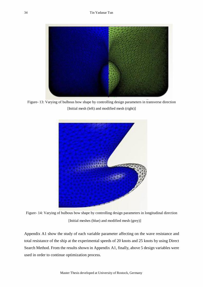
As above, there are 5 design parameters for optimization process. In Figure-13, the
examples of the effect of design parameters on changing the shape of hull form are illustrated.
34 Tin Yadanar Tun
Master Thesis developed at University of Rostock, Germany
Figure- 13: Varying of bulbous bow shape by controlling design parameters in transverse direction
[Initial mesh (left) and modified mesh (right)]
Figure- 14: Varying of bulbous bow shape by controlling design parameters in longitudinal direction
[Initial meshes (blue) and modified mesh (grey)]
Appendix A1 show the study of each variable parameter affecting on the wave resistance and
total resistance of the ship at the experimental speeds of 20 knots and 25 knots by using Direct
Search Method. From the results shown in Appendix A1, finally, above 5 design variables were
used in order to continue optimization process.
Ship Hull Optimization in Calm Water and Moderate Sea States 35
“EMSHIP” Erasmus Mundus Master Course, period of study September 2014 – February 2016
5. COMPUTATIONAL FLUID DYNAMICS (CFD) METHOD
In assessment of ship hull’s hydrodynamic performance optimization, CFD solvers play an
important role to compute the flow fields around the hull for different operation conditions.
The accuracy, computation time and reliability are to be considered while choosing CFD
solver for the optimizing process. There are a lot of effective, reliable and fast CFD tools for
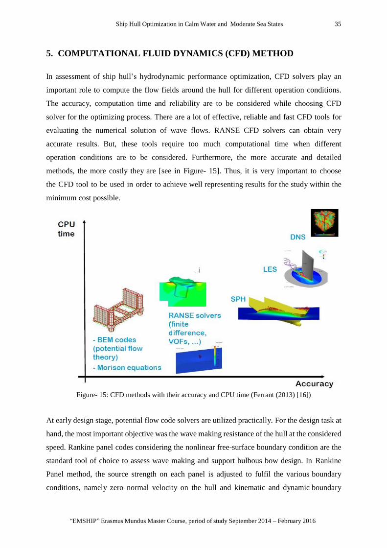
evaluating the numerical solution of wave flows. RANSE CFD solvers can obtain very
accurate results. But, these tools require too much computational time when different
operation conditions are to be considered. Furthermore, the more accurate and detailed
methods, the more costly they are [see in Figure- 15]. Thus, it is very important to choose
the CFD tool to be used in order to achieve well representing results for the study within the
minimum cost possible.
Figure- 15: CFD methods with their accuracy and CPU time (Ferrant (2013) [16])
At early design stage, potential flow code solvers are utilized practically. For the design task at
hand, the most important objective was the wave making resistance of the hull at the considered
speed. Rankine panel codes considering the nonlinear free-surface boundary condition are the
standard tool of choice to assess wave making and support bulbous bow design. In Rankine
Panel method, the source strength on each panel is adjusted to fulfil the various boundary
conditions, namely zero normal velocity on the hull and kinematic and dynamic boundary

36 Tin Yadanar Tun
Master Thesis developed at University of Rostock, Germany
conditions on the water surface. The ship’s dynamic floating position and the wave
formation are computed iteratively. After each iteration step, the geometry of the free surface
is updated and the sinkage, trim, heel are adjusted. The calculations are considered to be
converged when all forces and moments are in balance and all boundary conditions are fulfilled.
Having determined the source strengths, the pressure and velocity at each point of the flow field
can be calculated. The wave resistance can be computed by integrating the pressure over wetted
surface of the hull.
In potential flow theory, viscous effects such as a recirculation zone at the stern cannot be
calculated correctly. However, in hull optimization studies, the focus is on the forebody, to be
precise, on the bulbous bow shape where potential flow approximates the real conditions well.
The total resistance is predicted on the basis of the non-viscous resistance components from the
CFD simulation and an estimate of the viscous components by the ITTC method which
may optionally be based on local flow properties, or by an accompanying boundary layer
computation.
In this case, potential flow code GL Rankine developed by DNV-GL was used to calculate the
wave resistance and total resistance in steady flow computation and added resistance in waves
for seakeeping analysis.
5.1. GL Rankine Solver
The program GL Rankine can be used for the following computations [18]:
resistance in calm water, taking into account shallow water and channel walls
dynamic squat in calm water, taking into account shallow water and channel walls
linear transfer functions of ship motions in regular waves
sectional loads, relative motions and accelerations in waves
mapping of pressure distributions onto nodes of a finite-element mesh
hydrodynamic interaction of ships with the same forward speed and course
5.1.1. Use of GL Rankine Solver
Since GL Rankine solver does not have Graphical User Interface (GUI), it has to be run with
executable xml file, which is called config.xml or other arbitrary name, in the command line.
This file includes all the command for computation and input and output files such as
geometry of hull form or result files.
Ship Hull Optimization in Calm Water and Moderate Sea States 37
“EMSHIP” Erasmus Mundus Master Course, period of study September 2014 – February 2016
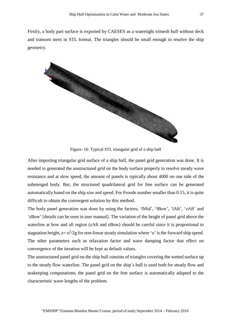
Firstly, a body part surface is exported by CAESES as a watertight trimesh hull without deck
and transom stern in STL format. The triangles should be small enough to resolve the ship
geometry.
Figure- 16: Typical STL triangular grid of a ship half
After importing triangular grid surface of a ship half, the panel grid generation was done. It is
needed to generated the unstructured grid on the body surface properly to resolve steady wave
resistance and at slow speed, the amount of panels is typically about 4000 on one side of the
submerged body. But, the structured quadrilateral grid for free surface can be generated
automatically based on the ship size and speed. For Froude number smaller than 0.15, it is quite
difficult to obtain the convergent solution by this method.
The body panel generation was done by using the factors; ‘lMid’, ‘lBow’, ‘lAft’, ‘zAft’ and
‘zBow’ [details can be seen in user manual]. The variation of the height of panel grid above the
waterline at bow and aft region (zAft and zBow) should be careful since it is proportional to
stagnation height, z= u2/2g for non-linear steady simulation where ‘u’ is the forward ship speed.
The other parameters such as relaxation factor and wave damping factor that effect on
convergence of the iteration will be kept as default values.
The unstructured panel grid on the ship hull consists of triangles covering the wetted surface up
to the steady flow waterline. The panel grid on the ship’s hull is used both for steady flow and
seakeeping computations; the panel grid on the free surface is automatically adapted to the
characteristic wave lengths of the problem.

38 Tin Yadanar Tun
Master Thesis developed at University of Rostock, Germany
Figure- 17: Typical panels generated by GL Rankine on a STL surface
After the panel grid generation for the hull underwater surface, the rectangular panel grids
generation of free surface was created automatically depending on the ship size and forward
speed.
Figure- 18: Automatically created structured free surface mesh in GL Rankine depending on speed

Ship Hull Optimization in Calm Water and Moderate Sea States 39
“EMSHIP” Erasmus Mundus Master Course, period of study September 2014 – February 2016
The nonlinear part of GL Rankine predicts the steady flow around a ship using nonlinear free
surface condition. The fluid is assumed to be inviscid, incompressible and irrotational.
Therefore a velocity potential exists, which has to fulfil the Laplace equation (conservation of
mass) as well as kinematic and a dynamic boundary conditions on the free surface (‘no flow
through the surface’ and ‘atmospheric pressure at the surface’, respectively).
Because the free surface boundary condition is nonlinear an iterative solution is required. An
under relaxed Newton-like iteration for the residuum is used. After determining the potential,
the forces and moments acting on the ship are computed by integration and obtained the wave
resistance, frictional resistance ( calculated by ITTC 1978) and total resistance of the vessel in
calm water condition.
For motion in waves, forces and moments acting on the ship surface depends linearly on the
incoming wave amplitudes for this method in linear response computation. By superimposing
the potential from the stationary problem and the potential of periodical flow which oscillates
with the wave frequency, the total potential needed for seakeeping analysis is calculated.
The method GL Rankine calculates ship motions and loads in waves, taking into account
interaction between the steady flow at constant forward speed and the periodic flow in waves.
The method is based on the linearization of the flow and ship motions due to incoming waves
with respect to the nonlinear steady flow produced by the ship motion in calm water with
constant speed, taking into account ship wave and dynamic squat. Therefore, seakeeping
computations are preceded by the solution of the steady flow problem.
The seakeeping contributions, considered up to first order, depend linearly on wave
amplitude, while the steady flow solution is fully nonlinear with respect to free surface
deformations, dynamic trim and sinkage and all boundary conditions. In addition, quadratic
transfer functions (i.e., forces and moments proportional to wave amplitude squared) are
computed to obtain added resistance and side drift force in waves.
The detailed explanation about how to coupled GL Rankine software connector with CAESES
was omitted in this thesis. The set up input XML file for steady flow computation and
seakeeping computation are shown in Appendix A2.
After the set-up for GL Rankine coupled with CAESES is done, detailed analysis of initial base
design has to be performed such as implying grid variation studies, convergence test and
accuracy check for the CFD analysis with experimental data in both calm water and in waves.
The results for each analysis can be seen in the sections 5.2 and 5.3.

40 Tin Yadanar Tun
Master Thesis developed at University of Rostock, Germany
5.2. Mesh Dependency on Numerical Results
In this part, the variation of CW coefficients in base model for Froude numbers of 0.174, 0.200
and 0.218, which correspond with ship speed of 20 knots, 23 knots and 25knots respectively,
will be checked for different hull grids. While changing the hull grid parameters, only the grid
length at the bow, mid and aft region will be changed. The variation of the height of panel grid
above the waterline at bow and aft region should be careful since it is proportional to stagnation
height, z= V2/2g for non-linear steady simulation. The other parameters such as relaxation factor
and wave damping factor that effect on convergence of the iteration will be kept as default
values.
Table - 2: Variation of grid parameters
Parameters
mesh 1
mesh 2
mesh 3
mesh 4
mesh 5
lMid
5
4
4
3.5
3
lBow
3
3
2.5
2.5
2
lAft
3
3
2.5
2.5
2
According to GL Rankine user manual, zAft = min (0.3 z, lAft) and zBow = min (0.5z to 1.0z,
lBow), where LAft = approximate grid length at aft region, lBow= approximate grid length at
bow region and z = u2/2g. According to the variation of zAft and zBow for different Froude
numbers, the number of panel generated of the hull is also different as shown in Table 3.
Table - 3: Number of Panels for Different Froude Numbers
Number of panels
Fn Mesh 1 Mesh 2 Mesh 3 Mesh 4 Mesh 5
0.174 2204 2965 3383 3888 5374
0.200 2312 3008 3424 3943 5527
0.218 2299 3048 3409 4004 5527
The free surface mesh is generated by default parameter according to different forward speed.
The free surface mesh around the hull for resistance calculation is generated as the structured
rectangular mesh.

Ship Hull Optimization in Calm Water and Moderate Sea States 41
“EMSHIP” Erasmus Mundus Master Course, period of study September 2014 – February 2016
Table - 4: Wave resistance coefficients for different mesh
Cw x e4(-) mesh1 mesh2 mesh3 mesh4 mesh5
Fn=0.174 1.3668 1.4863 1.4530 1.2277 1.2864
Fn=0.200 1.3753 1.3065 1.4516 1.2307 1.1362
Fn=0.218 1.8082 1.8784 2.1613 1.9535 1.4200
Figure- 19: Mesh Dependency for different Froude Numbers
While changing the mesh parameters, it should be noted that the maximum number of panels
generated below waterline is 10000 as default. Table 4 and Fig.19 show the wave resistance
coefficient for different mesh at Fr =0.174, 0.200, 0.218. It can be seen that the mesh
dependency is quite sensitive to the numerical results of wave resistance coefficient obtained
from GL Rankine solver.
For panel grid generation of the model, it should be nice to follow the standard recommendation
such as 1% of LPP of ship for panel size in middle section and 0.7% for that in forward or aft
section.
As summary, the final mesh of hull panel generation is chosen for mesh 3 with LAft, LBow
= 0.7% of LPP = 2.5 m and LMid = 1% of LPP = 4m [approximately 3500 panels on
hull, approximate computation time= 15 minutes for each simulation in Intel® Core™ i5-
3230M CPU @ 2.60GHz, RAM 4GB].
All the remaining works such as verification with experimental data and optimization processes
will be done with the same mesh parameters [as shown above- mesh3].
42 Tin Yadanar Tun
Master Thesis developed at University of Rostock, Germany
5.3. Validation of Numerical Results with Experimental Data
After the mesh parameters analysis was done, the coupling of GL Rankine config file with
CAESES was fixed and validated with the experimental results that are done in in the model
test basins SVA Potsdam (resistance and propulsion tests), Nietzschmann (2010), and HSVA
(roll decay tests), Schumacher (2011) in order to explore the accuracy of the results that come
out from GL Rankine solver.
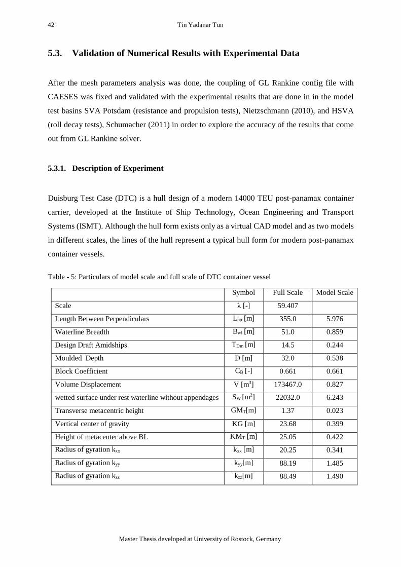
5.3.1. Description of Experiment
Duisburg Test Case (DTC) is a hull design of a modern 14000 TEU post-panamax container
carrier, developed at the Institute of Ship Technology, Ocean Engineering and Transport
Systems (ISMT). Although the hull form exists only as a virtual CAD model and as two models
in different scales, the lines of the hull represent a typical hull form for modern post-panamax
container vessels.
Table - 5: Particulars of model scale and full scale of DTC container vessel
Symbol Full Scale Model Scale
Scale λ [-] 59.407
Length Between Perpendiculars Lpp [m] 355.0 5.976
Waterline Breadth Bwl [m] 51.0 0.859
Design Draft Amidships TDm [m] 14.5 0.244
Moulded Depth D [m] 32.0 0.538
Block Coefficient CB [-] 0.661 0.661
Volume Displacement V [m3] 173467.0 0.827
wetted surface under rest waterline without appendages SW [m2] 22032.0 6.243
Transverse metacentric height GMT[m] 1.37 0.023
Vertical center of gravity KG [m] 23.68 0.399
Height of metacenter above BL KMT [m] 25.05 0.422
Radius of gyration kxx kxx [m] 20.25 0.341
Radius of gyration kyy kyy[m] 88.19 1.485
Radius of gyration kzz kzz[m] 88.49 1.490
Ship Hull Optimization in Calm Water and Moderate Sea States 43
“EMSHIP” Erasmus Mundus Master Course, period of study September 2014 – February 2016
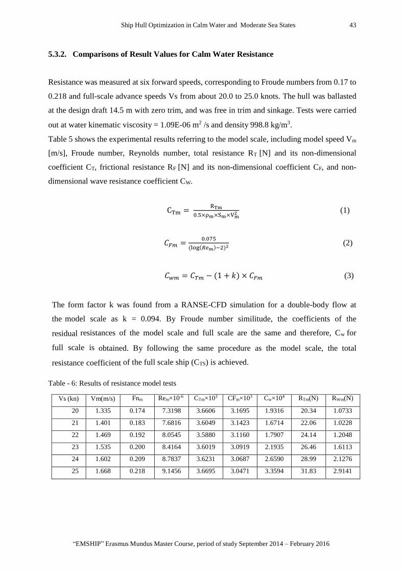
5.3.2. Comparisons of Result Values for Calm Water Resistance
Resistance was measured at six forward speeds, corresponding to Froude numbers from 0.17 to
0.218 and full-scale advance speeds Vs from about 20.0 to 25.0 knots. The hull was ballasted
at the design draft 14.5 m with zero trim, and was free in trim and sinkage. Tests were carried
out at water kinematic viscosity = 1.09E-06 m2 /s and density 998.8 kg/m3.
Table 5 shows the experimental results referring to the model scale, including model speed Vm
[m/s], Froude number, Reynolds number, total resistance RT [N] and its non-dimensional
coefficient CT, frictional resistance RF [N] and its non-dimensional coefficient CF, and non-
dimensional wave resistance coefficient CW.
CTm = RTm
0.5×ρm×Sm×Vm2 (1)
𝐶𝐹𝑚 =0.075
(log(𝑅𝑒𝑚)−2)2 (2)
𝐶𝑤𝑚 = 𝐶𝑇𝑚 − (1 + 𝑘) × 𝐶𝐹𝑚 (3)
The form factor k was found from a RANSE-CFD simulation for a double-body flow at
the model scale as k = 0.094. By Froude number similitude, the coefficients of the
residual resistances of the model scale and full scale are the same and therefore, Cw for
full scale is obtained. By following the same procedure as the model scale, the total
resistance coefficient of the full scale ship (CTS) is achieved.
Table - 6: Results of resistance model tests
Vs (kn) Vm(m/s) Fnm Rem×10-6 CTm×103
CFm×103 Cw×104
RTm(N) RWm(N)
20 1.335 0.174 7.3198 3.6606 3.1695 1.9316 20.34 1.0733
21 1.401 0.183 7.6816 3.6049 3.1423 1.6714 22.06 1.0228
22 1.469 0.192 8.0545 3.5880 3.1160 1.7907 24.14 1.2048
23 1.535 0.200 8.4164 3.6019 3.0919 2.1935 26.46 1.6113
24 1.602 0.209 8.7837 3.6231 3.0687 2.6590 28.99 2.1276
25 1.668 0.218 9.1456 3.6695 3.0471 3.3594 31.83 2.9141

44 Tin Yadanar Tun
Master Thesis developed at University of Rostock, Germany
For the range of Froude numbers used in experimental data, the CFD simulations in GL Rankine
for the final mesh panel hull and free surface are performed to compute non-dimensional
resistance coefficients (CT, CF and CW). The results are as follow in Table 7.
Table - 7: Results of GL Rankine Simulations
Parameters Base Model simulation with final mesh
Vs [knots] 20 21 22 23 24 25
lMid[m] 4 4 4 4 4 4
lBow [m] 2.5 2.5 2.5 2.5 2.5 2.5
lAft [m] 2.5 2.5 2.5 2.5 2.5 2.5
zBow [m] 2.5 2.5 2.5 2.5 2.5 2.5
zAft [m] 1.62 1.78 1.96 2.14 2.33 2.5
no. of panels 3383 3339 3346 3424 3323 3409
FS no. of panels 2503 2142 1809 1504 1296 1058
Trim(degree) 0.056 0.065 0.074 0.083 0.09 0.1
Sinkage(m) -0.235 -0.262 -0.292 -0.322 -0.355 -0.389
Wetted surface(m2)
22077
22078
22084
22087
22097
22109
Cw ×104 1.4530 1.2799 1.3522 1.4516 1.5874 2.1613
Figure- 20: Comparison of Wave Resistance Coefficients (Cw)

Ship Hull Optimization in Calm Water and Moderate Sea States 45
“EMSHIP” Erasmus Mundus Master Course, period of study September 2014 – February 2016
The comparison of the numerical results simulated by GL Rankine and the experimental results
performed by HSVA are described along with the results obtained from ShipFlow and RANSE
simulations in Fig.20. It can be seen that the numerical simulation was done for 6 different
forward speeds and its curve shows the same curvature as experimental data.
In order to compare the total resistance of the vessel in calm water condition, the form factor of
k= 0.117 (obtained from University of Duisburg, Personal Communication) was used for
full scale.
Figure- 21: Comparison of resistance in calm water condition
The frictional resistance has small variation due to the difference of the wetted surface area
and also for the wave resistance. By using k=0.117, the total resistance at 20 knots has the
decrement of 1.5% in numerical results compared to that in experimental results, while the
total resistance at 25 knots is reduced 6% in simulation. These differences are in the range of
acceptable limit and it can be said that GL Rankine has the relevant accuracy.
5.3.3. Comparisons of Result Values for Wave Added Resistance
Model tests for added resistance in waves use either self-propelled or towed models.
Self- propelled models eliminate the influence of the towing equipment on model motions;
however, the influence of motions and waves on the thrust deduction factor (required to
estimate the added resistance) remains a factor of uncertainty. Towed models have either
restrained surge motion or they are connected by soft springs to the towing carriage.
Restraining the surge motion may influence added resistance, especially if it interferes with

46 Tin Yadanar Tun
Master Thesis developed at University of Rostock, Germany
pitch and heave motions. Thus, the arrangement with springs appears more appropriate.
Another difficulty with experiments for added resistance in waves is that added resistance
(average longitudinal force over time) is small compared to the amplitude of force
variations. Thus, errors in measuring these forces might be comparable to or even exceed
the average force itself. Further, added resistance is sensitive to the quality of wave
generation and wave measurement, especially in short waves, because, unlike linear
reactions, added resistance depends on wave amplitude squared [5].
The towing test in regular waves was performed at the draught of 14.5 m with a DTC model
at the speed of 16 knots. The wave added resistance (RAW) is achieved by extracting the
calm water resistance from the total resistance of the model in waves. The transfer function
and the non-dimensional coefficient of the wave added resistance are computed by using the
Equations. 4 and 5. Assuming the wave added resistance coefficients of both model and full
scale ship are the same, the transfer function of wave added resistance of the DTC is
obtained by using the same equations as in model scale.
Transfer function of R𝐴𝑊 = RAW
ζa2 (4)
Non − dimensional added resistance coefficient = 𝐶𝐴𝑊 =RAW
ρ.g.(𝐵2
𝐿𝑤𝑙)ζa
2 (5)
The following result table shows the added resistance coefficient obtained from Experiments
and RANSE CFD results using Comet for design draft 14.5m at 16 knots forward speed
[Sebastian, personal communication].
Table - 8: DTC added resistance coefficient results

Ship Hull Optimization in Calm Water and Moderate Sea States 47
“EMSHIP” Erasmus Mundus Master Course, period of study September 2014 – February 2016
For the numerical results, the simulation is done by GL Rankine solver with the same wave
amplitudes as the experiment in head waves (180˚). The comparison is shown in Fig. 22 for the
speed of 16 knots at T=14.5m, describing the wave added resistance (CAW) versus the
ratio between wavelengths of incoming waves to ship length waterline.
Figure- 22: Comparison of added wave resistance coefficient (T=14.5m, Vs = 16 knots)
It is observed that the large difference between results of the test evaluations, especially in short
waves. The RANSE computations are quite similar to experimental results and to the results of
the potential code in medium and long waves. But they show relative errors in the short
waves region. This demonstrates the inherent difficulty to obtain reliable estimates of added
resistance in short waves.
The trends for the results have a certain amount of similarity. The potential flow solver GL
Rankine can deliver inaccurate results, especially for full hull forms and short waves, for
which the added resistance is increasingly affected by the viscous effects. The potential flow
theory based GL Rankine method is preferred over RANS code with respect to the
computational effort.
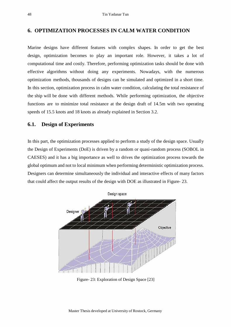
48 Tin Yadanar Tun
Master Thesis developed at University of Rostock, Germany
6. OPTIMIZATION PROCESSES IN CALM WATER CONDITION
Marine designs have different features with complex shapes. In order to get the best
design, optimization becomes to play an important role. However, it takes a lot of
computational time and costly. Therefore, performing optimization tasks should be done with
effective algorithms without doing any experiments. Nowadays, with the numerous
optimization methods, thousands of designs can be simulated and optimized in a short time.
In this section, optimization process in calm water condition, calculating the total resistance of
the ship will be done with different methods. While performing optimization, the objective
functions are to minimize total resistance at the design draft of 14.5m with two operating
speeds of 15.5 knots and 18 knots as already explained in Section 3.2.
6.1. Design of Experiments
In this part, the optimization processes applied to perform a study of the design space. Usually
the Design of Experiments (DoE) is driven by a random or quasi-random process (SOBOL in
CAESES) and it has a big importance as well to drives the optimization process towards the
global optimum and not to local minimum when performing deterministic optimization process.
Designers can determine simultaneously the individual and interactive effects of many factors
that could affect the output results of the design with DOE as illustrated in Figure- 23.
Figure- 23: Exploration of Design Space [23]

Ship Hull Optimization in Calm Water and Moderate Sea States 49
“EMSHIP” Erasmus Mundus Master Course, period of study September 2014 – February 2016
Appendix A3 shows the sampling of design space obtained from SOBOL with 150 designs in
order to get the feasible design with all ranges of design variables. With these results from
design of experiment, the best design can be selected and on it, the optimization method
performed.
6.2. Single Objective Optimization
For single objective optimization process, Local Optimization Efficient method in CAESES/
Dakota interface was used starting from the initial design selection from Design of Experiments
(SOBOL). This method is surrogate-based local optimization. For the initial surrogate model,
data is taken from Design of Experiments. During the run, the surrogate model is iteratively
fine-tuned: the optimum design from the local search is evaluated and the information is added
to the surrogate model – which step by step increases the quality of the model.
1st
Case - minimize total resistance at V=15.5knots at design draft of 14.5m
The Figure 24 presents the results for the optimization process together with the designs
obtained on the DoE study, displayed by their indexes (order of creation) and in the ordinate
is the difference in total resistance (%) relative to the base model.
𝐷𝑖𝑓𝑓𝑒𝑟𝑒𝑛𝑐𝑒 𝑖𝑛 𝑅𝑇(%) = 𝐷𝑒𝑠𝑖𝑔𝑛 𝑅𝑇 − 𝐵𝑎𝑠𝑒 𝑅𝑇
𝐵𝑎𝑠𝑒 𝑅𝑇
× 100% (6)
Figure- 24: Single objective optimization at 15.5 knots
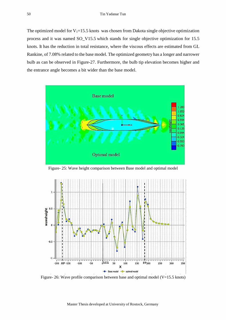
50 Tin Yadanar Tun
Master Thesis developed at University of Rostock, Germany
The optimized model for V1=15.5 knots was chosen from Dakota single objective optimization
process and it was named SO_V15.5 which stands for single objective optimization for 15.5
knots. It has the reduction in total resistance, where the viscous effects are estimated from GL
Rankine, of 7.08% related to the base model. The optimized geometry has a longer and narrower
bulb as can be observed in Figure-27. Furthermore, the bulb tip elevation becomes higher and
the entrance angle becomes a bit wider than the base model.
Figure- 25: Wave height comparison between Base model and optimal model
Figure- 26: Wave profile comparison between base and optimal model (V=15.5 knots)

Ship Hull Optimization in Calm Water and Moderate Sea States 51
“EMSHIP” Erasmus Mundus Master Course, period of study September 2014 – February 2016
Figure- 27: Base model and optimal model comparison (V =15.5 knots)
(initial mesh – yellow and optimal model mesh- blue)
2nd Case - minimize total resistance at V=18 knots at design draft of 14.5m
The same procedure is applied to optimize the model at 18 knots with Dakota/ Local
optimization efficient strategy. Figure-28 presents the results for the optimization process
together with the designs obtained on the DoE study, displayed by their indexes (order of
creation) and in the ordinate is the difference in total resistance (%) relative to the base model
for 18 knots.
Figure- 28: Single objective optimization at 18 knots

52 Tin Yadanar Tun
Master Thesis developed at University of Rostock, Germany
In comparison with based model, the optimal model for V=18 knots has a reduction of 3.97%
in total resistance of the ship. The optimized geometry has a bit shorter and narrower bulb as
can be observed in Figure-30. Furthermore, the bulb tip elevation becomes higher and the
entrance angle becomes wider than the base model.
Figure- 29: Wave cut comparison between base and optimal model (V=18 knots)
Figure- 30: Base model and optimal model comparison (V =18 knots)
(initial mesh – yellow and optimal model mesh- blue)

Ship Hull Optimization in Calm Water and Moderate Sea States 53
“EMSHIP” Erasmus Mundus Master Course, period of study September 2014 – February 2016
When comparing both models, optimized for V1 and V2 in both operating conditions, the results
can be observed as following in Figure- 31.
Figure- 31: Comparison of Single objective optimization for 15.5 knots and 18 knots
6.3. Single Objective Optimization with Weighted Functions
Multi-objective optimization can be performed by using the weighted function in the single
objective optimization functions. For the consideration of two different operational conditions
as objective function on the optimization process, several techniques were used where the
conditions are defined by the variation of the velocity (V1= 15.5 knots and V2= 18 knots). A
single objective optimization was performed in each case by surrogate-based local optimization
method and the multi-objective function (MoF) is defined as following:
MoF = α × RTV1 + (1-α) × RTV2 (6)
Where, RTV1 and RTV2 are total resistance at the speeds of V1= 15.5 knots and V2= 18 knots
respectively and α is the weight function coefficient (0<α < 1).
If α = 0 or α = 1, it is a single objective problem where only one condition is considered and the
results would be similar to those observed previously in Section 6.2. Three different values for
the weight coefficients were considered:
i. α = 0.25
ii. α = 0.50
iii. α = 0.75

54 Tin Yadanar Tun
Master Thesis developed at University of Rostock, Germany
6.3.1. α = 0.25
The weight of 0.25 means that 25% for the objective function is due to the resistance of the
vessel at velocity V1 and 75% related to the resistance of the vessel at velocity V2. It can also
be observed that the total resistance is reduced by 5.71% at 15.5 knots and 3.75 % at 18 knots
compared to the base model.
Figure- 32: Single objective optimization with α= 0.25
6.3.2. α = 0.50
The weight of 0.50 means that 50% for the objective function is due to the resistance of the
vessel at velocity V1 and 50% related to the resistance of the vessel at velocity V2. The total
resistance of the selected optimal model is reduced by 6.97% at 15.5 knots and 3.923 % at 18
knots compared to the base model.
Figure- 33: Single objective optimization with α= 0.50

Ship Hull Optimization in Calm Water and Moderate Sea States 55
“EMSHIP” Erasmus Mundus Master Course, period of study September 2014 – February 2016
Table - 9: Result summary for single objective optimization processes
V(knots) 15.5 18
RTV1 (kN) Diff (%) RTV2(kN) Diff(%)
Base model 1190.31 - 1489.08 -
SO_V18 α=0 Obj.fun: (0×RTV1) + (1×RTV2) 1145.08 -3.80 1430.01 -3.97
SO_α_0.25 α=0.25 Obj.fun: (0.25×RTV1) + (0.75×RTV2) 1122.40 -5.71 1430.28 -3.75
SO_α_0.50 α=0.50 Obj.fun: (0.5×RTV1) + (0.5×RTV2) 1107.34 -6.97 1430.67 -3.92
SO_α_0.75 α=0.75 Obj.fun: (0.75×RTV1) + (0.25×RTV2) 1106.89 -7.01 1430.89 -3.91
SO_V15.5 α=1.00 Obj.fun: (1×RTV1) + (0×RTV2) 1106.08 -7.08 1439.44 -3.33
6.3.3. α = 0.75
The weight of 0.75 means that 75% for the objective function is due to the resistance of the
vessel at velocity V1 and 25% related to the resistance of the vessel at velocity V2. The total
resistance of the selected optimal model is reduced by 7.00% at 15.5 knots and 3.91 % at 18
knots compared to the base model. It means that as the weight function coefficient used for V1
is increased, the reduction % of total resistance in V1 related to base model is also increased.
Figure- 34: Single objective optimization with α= 0.75
It can be observed in Table 9 that when varying the weight for RTV1, the higher is the
weight, the better is the improvement regarding to reduce total resistance at V1=15.5 knots. In
addition, the weighted method possible the optimization of the vessel for multiple
objectives (Minimization of RTV1 and RTV2), while using the surrogate-based local
optimization method.

56 Tin Yadanar Tun
Master Thesis developed at University of Rostock, Germany
6.4. Multi-objective Optimization
In general, there is no design in which all the functions are minimal as there is no unique
optimum design to a multi-objective optimization problem. However, there is a set of points
that represents the best compromise between the various objectives called Pareto Frontier.
Genetic algorithms are used to perform multi-objective optimization.
In this work, the surrogate-based global optimization strategy was used for multi-objective
optimization process in CAESES with Dakota. The advantage of this method is the speed of the
convergence of the design objective functions.
The multi-optimization process was performed for 350 designs in which 30 designs were chosen
as the samples for initial surrogate model. The process took 5 days approximately running in a
computer with the processor of Core ™ i7-2760QM CPU @ 2.40 GHz, RAM 8GB.
The template of Dakota surrogate based global optimization in accordance to the recommendation
of the specialist and developers of the CAESES for this study can be seen in Appendix A4.
Figure- 35: Convergence study of surrogate based global optimization
Finally, the results for the multi-objective optimization by means of genetic algorithms with
surrogate modal can be seen in Fig. 36. In Fig.37, the same results are presented with a zoom
in the area of interest, designs that have reduced resistance when compared to the base model
(negative values in the graphic). The total resistance related to base model is approximately
6.5% reduction at 15.5 knots and 3% reduction at 18 knots for the selected design 1
(MO_des270). And 6.2% and 4.31% reduction at 15.5 knots and 18 knots respectively for
selected deign 2 (MO_des 239).

Ship Hull Optimization in Calm Water and Moderate Sea States 57
“EMSHIP” Erasmus Mundus Master Course, period of study September 2014 – February 2016
Figure- 36: Multi-Objective Optimization (Dakota- SBGO)
Figure- 37: Multi-Objective Optimization (Dakota- SBGO) zoomed in design of interest

58 Tin Yadanar Tun
Master Thesis developed at University of Rostock, Germany
6.5. Sensitivity Analysis
Optimum designs via different methods were performed for two different speeds at the design
draft of 14.5 m. The robustness of the design is evaluated regarding the sensitivity to
uncertainties variations on the draft of the vessel. For the sensitivity analysis, the best achieved
designs of some of the optimization processes were selected and the RTV1 and RTV2 for several
draft values were studied. The selected designs for the sensitivity analysis are as follows:
(1) SO_V15.5 - the optimal design obtained for single objective optimization for RTV1
(2) SO_V18 - the optimal design obtained for single objective optimization for RTV2
(3) SO_α_0.25 - the optimal design obtained for single objective optimization
with weighted coefficient of 0.25
(4) SO_α_0.50 - the optimal design obtained for single objective optimization
with weighted coefficient of 0. 50
(5) SO_α_0.75 - the optimal design obtained for single objective optimization
with weighted coefficient of 0.75
(6) MO _des270 - the optimal design obtained from multi-objective optimization
(7) MO _des238 - the optimal design obtained from multi-objective optimization
Figure- 38: Sensitivity analysis of draft variation for selected designs at V1 = 15.5 knots
(Optimization was performed at T=14.5m)
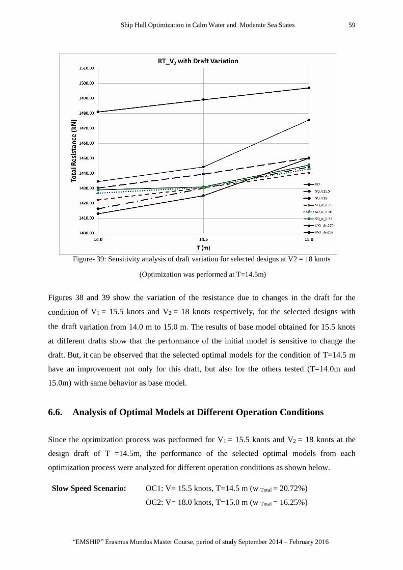
Ship Hull Optimization in Calm Water and Moderate Sea States 59
“EMSHIP” Erasmus Mundus Master Course, period of study September 2014 – February 2016
Figure- 39: Sensitivity analysis of draft variation for selected designs at V2 = 18 knots
(Optimization was performed at T=14.5m)
Figures 38 and 39 show the variation of the resistance due to changes in the draft for the
condition of V1 = 15.5 knots and V2 = 18 knots respectively, for the selected designs with
the draft variation from 14.0 m to 15.0 m. The results of base model obtained for 15.5 knots
at different drafts show that the performance of the initial model is sensitive to change the
draft. But, it can be observed that the selected optimal models for the condition of T=14.5 m
have an improvement not only for this draft, but also for the others tested (T=14.0m and
15.0m) with same behavior as base model.
6.6. Analysis of Optimal Models at Different Operation Conditions
Since the optimization process was performed for V1 = 15.5 knots and V2 = 18 knots at the
design draft of T =14.5m, the performance of the selected optimal models from each
optimization process were analyzed for different operation conditions as shown below.
Slow Speed Scenario: OC1: V= 15.5 knots, T=14.5 m (w Total = 20.72%)
OC2: V= 18.0 knots, T=15.0 m (w Total = 16.25%)
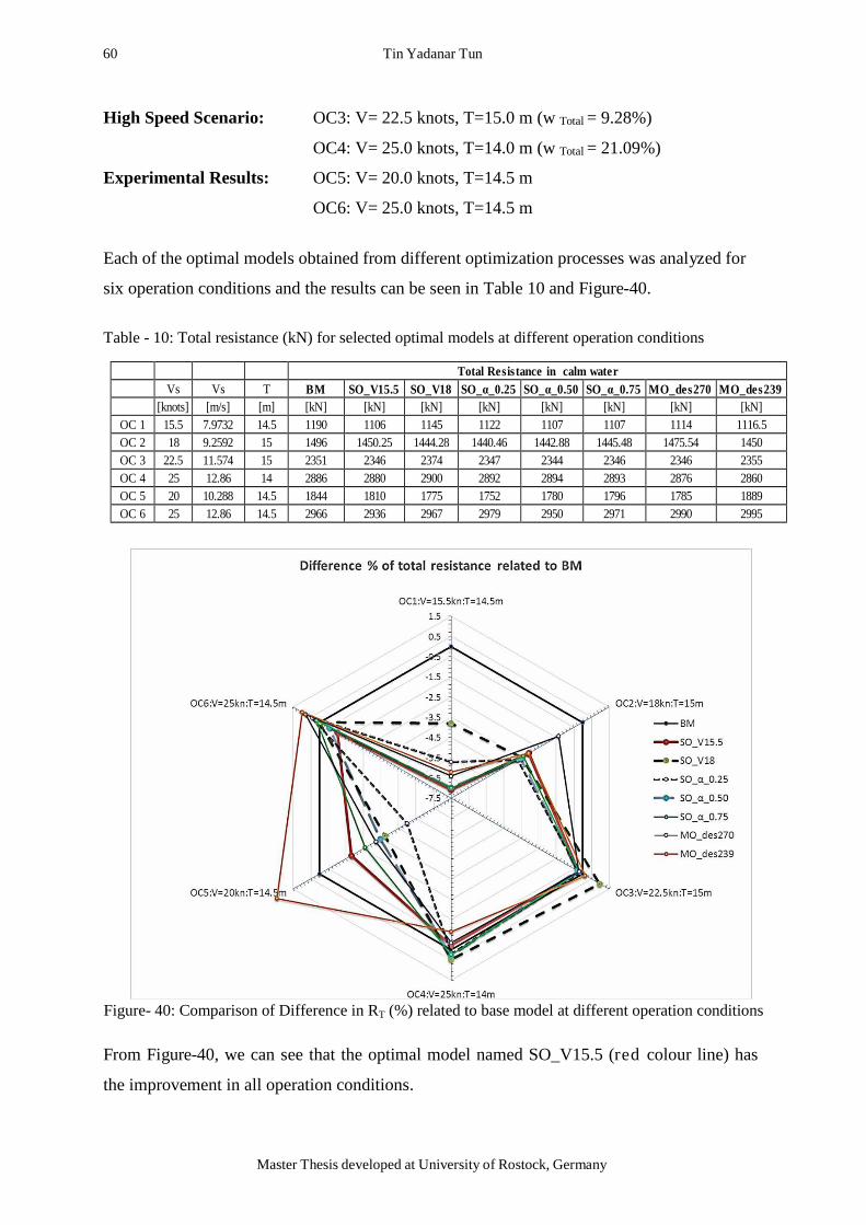
60 Tin Yadanar Tun
Master Thesis developed at University of Rostock, Germany
High Speed Scenario: OC3: V= 22.5 knots, T=15.0 m (w Total = 9.28%)
OC4: V= 25.0 knots, T=14.0 m (w Total = 21.09%)
Experimental Results: OC5: V= 20.0 knots, T=14.5 m
OC6: V= 25.0 knots, T=14.5 m
Each of the optimal models obtained from different optimization processes was analyzed for
six operation conditions and the results can be seen in Table 10 and Figure-40.
Table - 10: Total resistance (kN) for selected optimal models at different operation conditions
Total Resistance in calm water
Vs Vs T BM SO_V15.5 SO_V18 SO_α_0.25 SO_α_0.50 SO_α_0.75 MO_des270 MO_des239
[knots] [m/s] [m] [kN] [kN] [kN] [kN] [kN] [kN] [kN] [kN]
OC 1 15.5 7.9732 14.5 1190 1106 1145 1122 1107 1107 1114 1116.5
OC 2 18 9.2592 15 1496 1450.25 1444.28 1440.46 1442.88 1445.48 1475.54 1450
OC 3 22.5 11.574 15 2351 2346 2374 2347 2344 2346 2346 2355
OC 4 25 12.86 14 2886 2880 2900 2892 2894 2893 2876 2860
OC 5 20 10.288 14.5 1844 1810 1775 1752 1780 1796 1785 1889
OC 6 25 12.86 14.5 2966 2936 2967 2979 2950 2971 2990 2995
Figure- 40: Comparison of Difference in RT (%) related to base model at different operation conditions
From Figure-40, we can see that the optimal model named SO_V15.5 (red colour line) has
the improvement in all operation conditions.

Ship Hull Optimization in Calm Water and Moderate Sea States 61
“EMSHIP” Erasmus Mundus Master Course, period of study September 2014 – February 2016
7. SEAKEEPING ANALYSIS IN MODERATE SEA STATES
As one of the main objectives of this thesis, the analysis of added resistance due to waves has
to be done after optimization in calm water conditions. Since the container vessel has not been
built yet, the wave data and the study of sea states are done from statistical data of existing
similar vessels. This process is performed by specialists from University of Rostock. The wave
scenario data that the vessel has to deal with are resulted for all specific wave height (H1/3)
and wave period (T1) are chosen for three operating conditions covering 50.60% of the
total operating time by the vessel. The wave scenario data of one operation condition
[T =15m, V=18knots] can be seen as the scatter diagrams in Figure- 41.
Figure- 41: Scatter Diagram of wave data at T= 15m, V=18 knots
7.1. Added Wave Resistance Due to Head Waves for Initial Model
The most reliable way to determine the increase of resistance due to the effect of waves is to
carry out seakeeping tests in regular waves of constant wave height, and different wave lengths
and directions at various speeds according to ITTC 7.5-022-07-02.2 [19]. The added wave
resistance due to head wave for different wave period and wave height can be calculated by
the use of equation 7.

62 Tin Yadanar Tun
Master Thesis developed at University of Rostock, Germany
Where,
RAW = mean added resistance increase in long-crested irregular head waves
RAW / ζA2 = quadratic transfer function of the mean longitudinal drift force obtained from GL
Rankine
Sf (ω) = frequency spectrum, for ocean waves modified Pierson-Moskowitz type
The result of added wave resistance due to head waves for the initial model can be seen
in Figures 42 and 43 for different wave periods and significant wave heights.
Figure- 42: Added wave resistance due to head waves for the initial base model
(V = 15.5 knots, T=14.5m)

Ship Hull Optimization in Calm Water and Moderate Sea States 63
“EMSHIP” Erasmus Mundus Master Course, period of study September 2014 – February 2016
Figure- 43: Added wave resistance due to head waves for the initial base model
(V = 18.0 knots, T=14.5m)
The added wave resistance related to total resistance in calm water (%) for the area of
interest was calculated and shown in Figures. 44 and 45.
Figure- 44: Added wave resistance due to head waves for initial base model for area of interest only
(V = 15.5 knots, T=14.5m)

64 Tin Yadanar Tun
Master Thesis developed at University of Rostock, Germany
Figure- 45: Added wave resistance due to head waves for initial base model for area of interest only
(V = 18 knots, T=14.5m)
7.2. Added Wave Resistance Comparison of Optimal Models
Although the hull form has been optimized for two speeds in calm water condition, seakeeping
performance of each optimum design is checked by simulating the design in the selected sea
state with GL Rankine solver. In order to compare the seakeeping performance, each calm water
combination is added its most frequent sea state, which has the advantage of not increasing
the number of combinations of optimization process. Table 11 shows the wave scenario data
that the vessel has to deal with for two operating conditions.
Table - 11: Wave scenario data for two operation conditions
Operation Condition Speed , Vs Draft , T Peak Period, TP Significant Wave Height, H1/3
[-] [knots] [m] [sec] [m]
OC 1 15.5 14.5 12.5 1.25
OC 2 18 15 12.5 1.75
By using the most frequent wave height of each condition and the peak period observed from
wave spectrum, the added wave resistance was calculated for selected optimal models from
single objective optimization process in calm water conditions. The results of each model and
the difference % related to the base model (BM) were shown in Table 12. It can be seen that
the optimal models obtained from the optimization in calm water conditions at T=14.5m have
the improvement regarding to not only calm water resistance but also for added resistance in

Ship Hull Optimization in Calm Water and Moderate Sea States 65
“EMSHIP” Erasmus Mundus Master Course, period of study September 2014 – February 2016
waves for V1=15.5 knots while the added resistance in waves for V2=18 knots got the higher
results than the base model. But the total resistance in waves of different optimal models has
the improvement in both operational conditions.
Table - 12: Comparison of total resistance due to waves of optimum models at two speeds
Calm Water
Resistance
Added Wave
Resistance
Total
Resistance
Designs [kN] [kN] [kN]
BM 15.5 knots 1190 40.5 1230.5
18 knots 1489 87 1576
SO_V15.5
15.5 knots 1106 39.4 1145.4
Diff: from BM -7.06% -2.72% -6.92%
18 knots 1439 87.5 1526.5
Diff: from BM -3.36% 0.575% -3.14%
SO_V18
15.5 knots 1145 40 1185
Diff: from BM -3.78% -1.235% -3.7%
18 knots 1430 87.7 1517.7
Diff: from BM -3.96% 0.805% -3.7%
SO_α_0.25
15.5 knots 1122 40.2 1162.2
Diff: from BM -5.71% -0.74% -5.55%
18 knots 1430.3 87.4 1517.7
Diff: from BM -3.75% 0.46% -3.71%
SO_α_0.50
15.5 knots 1107.34 39.8 1147.14
Diff: from BM -6.97% -1.73% -6.77%
18 knots 1431 87.8 1518.8
Diff: from BM -3.92% 0.92% -3.63%
SO_α_0.75
15.5 knots 1107 40 1147
Diff: from BM -7.01% -1.235% -6.786%
18 knots 1431 87.9 1519
Diff: from BM -3.91% 1.034% -3.62%
MO_des 270
15.5 knots 1114 39.2 1153.2
Diff: from BM -6.41% -3.21% -6.282%
18 knots 1475 87.1 1562.1
Diff: from BM -1.37% 0.11% -0.9%
MO_des 239
15.5 knots 1116 39.8 1155.8
Diff: from BM -6.22% -1.73% -6.07%
18 knots 1425 87.6 1512.6
Diff: from BM -4.30% 0.69% -4.023%

66 Tin Yadanar Tun
Master Thesis developed at University of Rostock, Germany
7.3. Direct Optimization of Total Resistance in Waves
After the optimization of hull form in calm water conditions and analysis of added resistance in
waves for optimal hull forms were done, the direct optimization of total resistance in waves for
moderate sea states, summing the total resistance in calm water and added resistance due to
head waves, was performed. The optimization was done of the wave scenario as shown in
section 7.2 with the most frequent wave height and the peak period of 12.5s in the
wave direction of 180 degrees.
The set-up file for GL Rankine was coupled with CAESES for both steady flow and seakeeping
computations. The two result files obtained from GL Rankine gave the total resistance in calm
water condition and the added wave resistance for sea state and by summing up; the total
resistance in waves was calculated. Then, the model was optimized directly for the total
resistance in waves for two operation conditions, V1 = 15.5 knots, T1=14.5m and V2= 18 knots,
T2 = 15m.
In this stage of finding the total resistance in waves directly, the single objective optimization
with Dakota was omitted since the computation time in GL Rankine for both steady flow and
seakeeping computations took approximately one hour for each design variant. Therefore,
Design of Experiments was performed for 300 design variants by using only SOBOL in
CAESES and the best design was selected from 300 designs which give the minimum total
resistance in waves for the selected sea state.
The Figure 46 and 47 present the results of total resistance in waves for the designs obtained on
the DoE study, displayed by their indexes (order of creation) and in the ordinate of the
difference in total resistance (%) relative to the base model.

Ship Hull Optimization in Calm Water and Moderate Sea States 67
“EMSHIP” Erasmus Mundus Master Course, period of study September 2014 – February 2016
When compared to the base model, the optimal model for operation condition 1 (Index-208)
had the reduction of 7.494% in the total resistance in waves and that for operation condition 2
(Index-280) had the reduction of 2.1% in the total resistance in waves.
The comparison of the geometry of the bulbous bow for the selected optimal models for the two
operation conditions and the comparison of total resistance in waves related to base model at
different wave heading angles can be seen in the next section.
Figure- 46: DoEs by SOBOL and Optimal Model for V1 = 15.5 knots, T1=14.5m
Figure- 47: DoEs by SOBOL and Optimal Model for V2 = 18 knots, T2=15m

68 Tin Yadanar Tun
Master Thesis developed at University of Rostock, Germany
8. RESULTS AND ANALYSIS
8.1. State of the Art in Optimization for Calm Water Conditions
In Table 13, the number of CFD runs necessary to perform the optimization for each method is
presented side by side with final performance obtained (Total resistance in waves) relative to
the base model for the speed of V1 = 15.5 knots and V2 = 18 knots at the design draft of
T=14.5m.
Table - 13: Number of CFD runs and Total resistance in waves related to base model %
Design
CFD run
(DoE+Opt)
Performance
V1 V2
Op
tim
izati
on
in
Calm
Wate
r C
on
dit
ion
s
Single
Objective
DoE+ surrogate
based local
optimization
SO_V15.5
267
-6.92%
-3.14%
SO_V18
250
-3.7%
-3.7%
Multi-
Objective
S.Obj with
w=0.25
SO_α_0.25
254
-5.55%
-3.71%
S.Obj with w=0.5
SO_α_0.50
-6.77%
-3.63%
S.Obj with
w=0.75
SO_α_0.75
-6.786%
-3.82%
Dakota MOGA
(surrogate based
global
optimization)
MO_des 270
350
-6.282%
-0.9%
MO_des 239
-6.07%
-4.023%
From the results in Table 13, it can be observed that when the objective function is to minimize
the total resistance in V1= 15.5 knots, the greater the weighted function coefficient, the better
the improvement of the results of V1. When comparing the optimum designs obtained by the
several optimization processes some trends of the form characteristics are observed in Table 14.

Ship Hull Optimization in Calm Water and Moderate Sea States 69
“EMSHIP” Erasmus Mundus Master Course, period of study September 2014 – February 2016
Table - 14: Geometry trend of the optimized bulbous bow
Designs
Length
Width
Height
Bulb tangent
at top
( 0 deg for
Base
model)
Entrance
angle (0
deg for
base model)
Difference
in final
volume
SO_V15.5 23%longer 99%narrower 21%higher -1.8deg 35% wider -0.12%
SO_α_0.75 6%longer 97.8%narrower 93%higher 7deg 85% wider -0.12%
SO_α_0.50 11%longer 99.5%narrower 75%higher 5.3deg 99% wider -0.11%
SO_α_0.25 17%shorter 99%narrower 59%higher 9.5deg 63% wider -0.10%
SO_V18 12%shorter 97%narrower 70%higher 9.12deg 55% wider -0.13%
MO_des 270 8.3%shorter 99.3%narrower 39%lower -4.6deg 39% wider -0.13%
MO_des 239 99 %longer 99%narrower 72%higher 8.5deg 80% wider -0.15%
The analysis is performed by the relative value of the design variable that defines the geometry.
For example, the bulbous bow for the first case presents a value 99% narrower which means
that the parameter that controls the width of the bulb is in between the mean value (base
model) and the lower bound, in 99% of that range.
8.2. Optimal Model Selected from the Optimization in Calm Water
Considering the performance of the designs obtained with single objective and multi-objective
optimization processes, the design SO_V15.5 is selected as final optimal model. This model has
the improvement in total calm water resistance of 7.06% and 3.36% for 15.5 knots and 18 knots
respectively at the design draft T=14.5m . This model also has the improvements in different
operation conditions [Figure- 48].
Figure- 48: Comparison of Diff: % in RT for different operation conditions

70 Tin Yadanar Tun
Master Thesis developed at University of Rostock, Germany
Figure- 49: Wave pattern of the optimal and base hull form (V=15.5knots, T=14.5m)
Figure- 50: Wave Profile for Base and Optimum model (V=15.5knots, T=14.5m)

Ship Hull Optimization in Calm Water and Moderate Sea States 71
“EMSHIP” Erasmus Mundus Master Course, period of study September 2014 – February 2016
Figure- 51: Wave Cut at Y/LPP=0.2 for Base and Optimum model (V=15.5knots, T=14.5m)
The variation of the wave generated by the vessel can also be observed by the wave cut far from
the body presented in the Figure-51. The differences in the wave pattern and wave cut are
due to variations on the hull form as presented in Figure-52. In Figure-52, it can be observed
that only the forebody of the vessels present some differences. The bulbous bow is a bit
narrower and longer than the base model. The bulb tip elevation becomes a bit higher than the
base model.
Figure- 52: Base model and final optimal model comparison (V =15.5 knots, T= 14.5m)

72 Tin Yadanar Tun
Master Thesis developed at University of Rostock, Germany
In Figures 53 to 55, the total resistance of the vessel in calm water condition for initial
model and final optimal model are presented for three different drafts ( T= 14 m, 14.5 m,
15 m ) at the velocities from 15.5 knots to 25 knots.
Figure- 53: Total resistance of base model and optimal model at whole range of operational speeds at
T=14.5m [In the secondary axis the relative difference in percentage is presented]
Figure- 54: Total resistance of base model and optimal model at whole range of operational speeds at
T=14.0m

Ship Hull Optimization in Calm Water and Moderate Sea States 73
“EMSHIP” Erasmus Mundus Master Course, period of study September 2014 – February 2016
Figure- 55: Total resistance of base model and optimal model at whole range of operational speeds at
T=15.0m
The optimization process was performed for a fixed draft of 14.5 m, however the optimum
vessel present a good performance not only at this draft but also for different drafts
conditions. Leading to the conclusion, the optimized model has a level of sensitivity,
regarding uncertainties on the draft value, similar to the base model. In conclusion, the
selected design from the optimization presents a good behavior at variations on the draft,
and also has the improvement in the total resistance for the main operational velocities.
8.3. Optimal Model Selected from the Direct Optimization in Sea States
As in calm water condition, the final performance obtained (Total resistance in waves) relative
to the base model for the speed of V1 = 15.5 knots, T1=14.5m and V2 = 18 knots, T2=15m
was tabulated as following.
Table - 15: CFD runs and Total resistance in waves related to base model % in sea states
Design
CFD run
(DoE)
Performance
V1=15.5kn V2= 18 kn
Optimization in
sea states
DoE(SOBOL)
SO_Rt_OC1
(ID_208)
300
-7.5%
-1.36%
SO_Rt_OC2
(ID_280)
300
-4.88%
-2.1%

74 Tin Yadanar Tun
Master Thesis developed at University of Rostock, Germany
From the results in Table 15, it can be observed that when the objective function is to minimize
the total resistance in V1= 15.5 knots at T1=14.5m, the total resistance in waves have the
reduction of -7.5 % for the objective operation condition and -1.36% for the another operation
condition for the same optimal model. Similarly, when the objective function is to minimize the
total resistance in V2= 18 knots at T2=15m, the total resistance in waves have the reduction of
-4.88 % for the objective operation condition and -2.1% for another operation condition. It
means that the selected optimal models for each operation condition have the improvement in
the performance not only for the objective function but also for another function.
When comparing the optimum designs obtained by the two operation conditions, some
trends of the form characteristics are observed in Table 16.
Table - 16: Geometry trend of the optimized bulbous bow (optimization in sea states)
Bulbous bow characteristics
Designs
Length
Width
Height
Bulb tangent at top
( 0 deg for Base
model)
Entrance angle
(0 deg for base
model)
SO_Rt_OC1
(ID_208)
73%longer
87%narrower
27%higher
-3.56deg
61% wider
SO_Rt_OC2 (ID_280)
82%longer
72.5%narrower
87%higher
8deg
57% wider
As per table 16, the bulb is longer in length, narrower in width and higher in the bulb tip height
when compared to the base model. When the objective function is to minimize the total
resistance in waves for operation condition V1 =15.5 knots and T1=14.5m, the bulb tangent at
the top becomes flatter than the base model. But for the other objective function, that becomes
fuller than the base model. In order to get the faired incident waves due to the shape variation,
the wave entrance angle becomes 61% and 57% wider than the base model at the respective
operation condition.
8.3.1. Analysis of the Optimal Models for Different Wave Heading Angles
Since the direct optimization in sea states was performed only due to the head waves ( 180 deg)
for both operation conditions, the selected optimal models from SOBOL was analyzed
for different wave heading angles, such as 30 deg off bow and 60 deg off bow and compared
the performance for those angles with the base model.

Ship Hull Optimization in Calm Water and Moderate Sea States 75
“EMSHIP” Erasmus Mundus Master Course, period of study September 2014 – February 2016
The set-up file for seakeeping computation in GL Rankine was modified to calculate the
average drift force for different frequency range with the heading angle 180 deg, 150 deg and
120 deg. The result file obtained from the seakeeping computation was imported to the
MATLAB code, named ‘Added Resistance.m’, prepared by the author in order to compute the
maximum added wave resistance for the selected wave scenario. The detail of the
computation steps in MATLAB code can be seen in APPENDIX- A5.
Figure- 56: Added wave resistance/ Rt (Calm water) (%) for head waves
Figure- 57: Added wave resistance/ Rt (Calm water) (%) in seaway 30 deg off bow
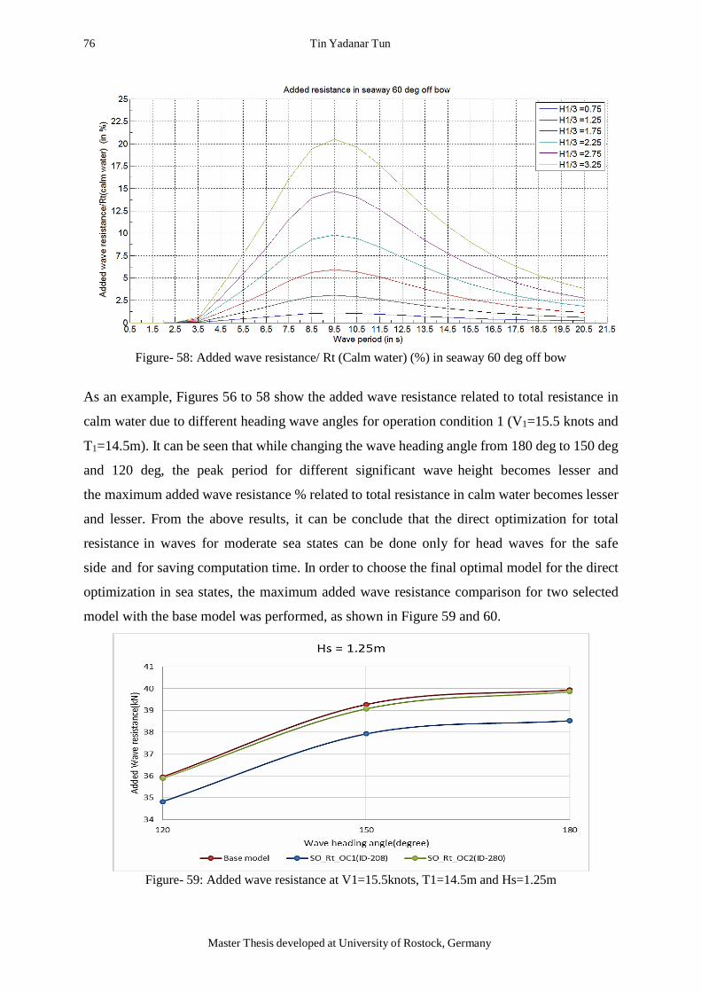
76 Tin Yadanar Tun
Master Thesis developed at University of Rostock, Germany
Figure- 58: Added wave resistance/ Rt (Calm water) (%) in seaway 60 deg off bow
As an example, Figures 56 to 58 show the added wave resistance related to total resistance in
calm water due to different heading wave angles for operation condition 1 (V1=15.5 knots and
T1=14.5m). It can be seen that while changing the wave heading angle from 180 deg to 150 deg
and 120 deg, the peak period for different significant wave height becomes lesser and
the maximum added wave resistance % related to total resistance in calm water becomes lesser
and lesser. From the above results, it can be conclude that the direct optimization for total
resistance in waves for moderate sea states can be done only for head waves for the safe
side and for saving computation time. In order to choose the final optimal model for the direct
optimization in sea states, the maximum added wave resistance comparison for two selected
model with the base model was performed, as shown in Figure 59 and 60.
Figure- 59: Added wave resistance at V1=15.5knots, T1=14.5m and Hs=1.25m

Ship Hull Optimization in Calm Water and Moderate Sea States 77
“EMSHIP” Erasmus Mundus Master Course, period of study September 2014 – February 2016
Figure- 60: Added wave resistance at V2=18knots, T2=15m and Hs=1.75m
From Figures 59 and 60, it shows that the optimal models selected from the direct optimization
in sea states for head waves (180 deg) by means of SOBOL method have the improvement in
other wave heading angles. But, the optimal model obtained from the objective function of
minimizing the total resistance in waves for operation condition 1 has the greater improvement
in both operation conditions when compared to the base model. Therefore, the optimal model
named SO_Rt_OC1 (Design Index-208 in SOBOL) was selected as the final optimal model for
the direct optimization in moderate sea states.
Figure- 61: Comparison of Geometry of Bulbous Bow in Longitudinal View
[ Base model – Yellow, Optimal Model – Grey]

78 Tin Yadanar Tun
Master Thesis developed at University of Rostock, Germany
Figure- 62: Comparison of Geometry of Bulbous Bow in Transverse View
[Base model – Yellow, Optimal Model – Blue]
Figure 61 and 62 show the comparison of the geometry between base model and the final
optimal model. The bulbous bow is a bit narrower and longer than the base model. The bulb tip
elevation becomes a bit higher than the base model [Details can be seen in Table 16].
In conclusion, the selected design from the direct optimization presents a good behavior at
variations of the wave heading angles and also has the improvement in the total resistance in
sea states for the main operational velocities.
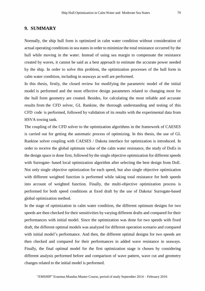
Ship Hull Optimization in Calm Water and Moderate Sea States 79
“EMSHIP” Erasmus Mundus Master Course, period of study September 2014 – February 2016
9. SUMMARY
Normally, the ship hull form is optimized in calm water condition without consideration of
actual operating conditions in sea states in order to minimize the total resistance occurred by the
hull while moving in the water. Instead of using sea margin to compensate the resistance
created by waves, it cannot be said as a best approach to estimate the accurate power needed
by the ship. In order to solve this problem, the optimization processes of the hull form in
calm water condition, including in seaways as well are performed.
In this thesis, firstly, the closed review for modifying the parametric model of the initial
model is performed and the most effective design parameters related to changing most for
the hull form geometry are created. Besides, for calculating the most reliable and accurate
results from the CFD solver, GL Rankine, the thorough understanding and testing of this
CFD code is performed, followed by validation of its results with the experimental data from
HSVA towing tank.
The coupling of the CFD solver to the optimization algorithms in the framework of CAESES
is carried out for getting the automatic process of optimizing. In this thesis, the use of GL
Rankine solver coupling with CAESES / Dakota interface for optimization is introduced. In
order to receive the global optimum value of the calm water resistance, the study of DoEs in
the design space is done first, followed by the single objective optimization for different speeds
with Surrogate- based local optimization algorithm after selecting the best design from DoE.
Not only single objective optimization for each speed, but also single objective optimization
with different weighted function is performed while taking total resistance for both speeds
into account of weighted function. Finally, the multi-objective optimization process is
performed for both speed conditions at fixed draft by the use of Dakota/ Surrogate-based
global optimization method.
In the stage of optimization in calm water condition, the different optimum designs for two
speeds are then checked for their sensitivities by varying different drafts and compared for their
performances with initial model. Since the optimization was done for two speeds with fixed
draft, the different optimal models was analyzed for different operation scenario and compared
with initial model’s performance. And then, the different optimal designs for two speeds are
then checked and compared for their performances in added wave resistance in seaways.
Finally, the final optimal model for the first optimization stage is chosen by considering
different analysis performed before and comparison of wave pattern, wave cut and geometry
changes related to the initial model is performed.

80 Tin Yadanar Tun
Master Thesis developed at University of Rostock, Germany
Table - 17: Performance Summary of the final optimal models for two operation conditions
Design
CFD run
(DoE+Opt)
Performance
V =15.5kn
T1=14.5m
V = 18 kn
T2=15m
Optimization in
calm water
condition
DoE+ surrogate
based local
optimization
SO_V15.5
267
-6.92%
-3.14%
Optimization in
sea states
DoE(SOBOL)
SO_Rt_OC1
(ID_208)
300
-7.5%
-1.36%
In the second stage, the direct optimization in moderate sea states was performed for the selected
wave scenario for two operation conditions. This process was performed only with the use of
SOBOL in CAESES for finding 300 design variants and selected the optimal model for
respective operation condition. Since the optimization was done only for head waves, the
performance of the two selected models was analyzed for the different wave heading
angles. The final optimal model for the direct optimization in moderate sea states was
chosen by comparing the performance at different heading angles which gives the minimum
total resistance in waves for the selected sea state.
As summary, table 17 shows the performance of the final optimal models chosen from the
optimization in calm water condition and direct optimization in moderate sea states compared
to the base model.
1 2
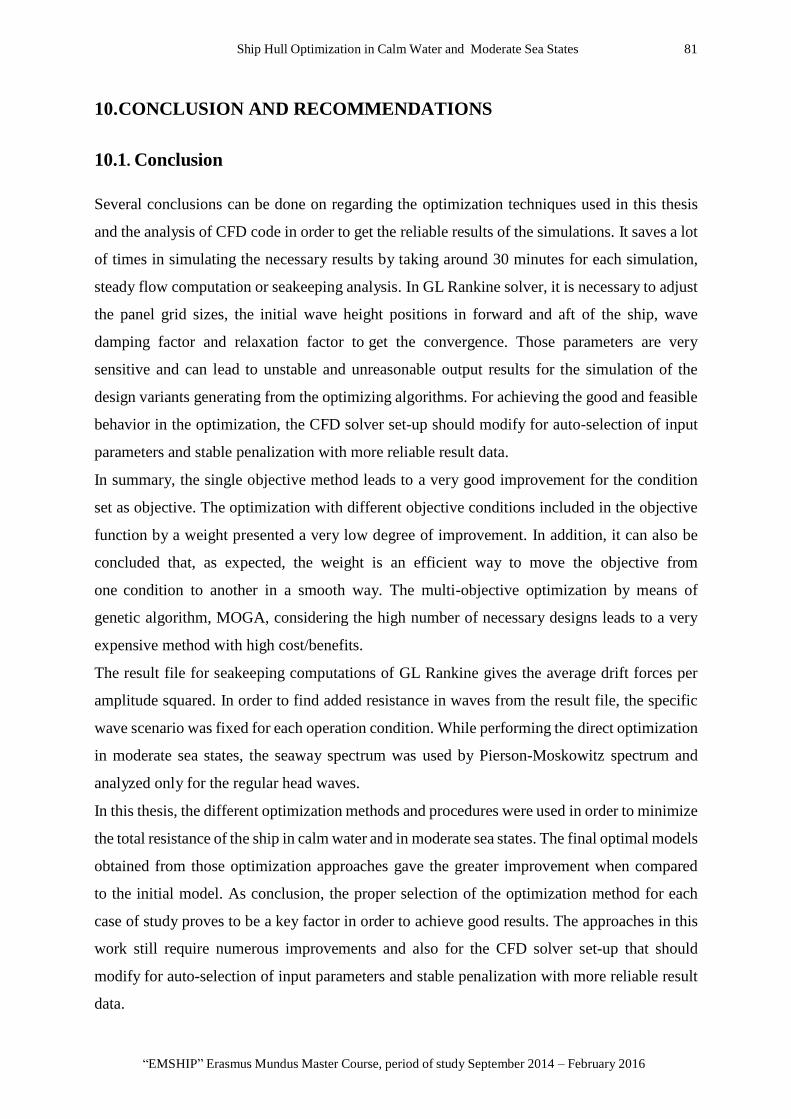
Ship Hull Optimization in Calm Water and Moderate Sea States 81
“EMSHIP” Erasmus Mundus Master Course, period of study September 2014 – February 2016
10. CONCLUSION AND RECOMMENDATIONS
10.1. Conclusion
Several conclusions can be done on regarding the optimization techniques used in this thesis
and the analysis of CFD code in order to get the reliable results of the simulations. It saves a lot
of times in simulating the necessary results by taking around 30 minutes for each simulation,
steady flow computation or seakeeping analysis. In GL Rankine solver, it is necessary to adjust
the panel grid sizes, the initial wave height positions in forward and aft of the ship, wave
damping factor and relaxation factor to get the convergence. Those parameters are very
sensitive and can lead to unstable and unreasonable output results for the simulation of the
design variants generating from the optimizing algorithms. For achieving the good and feasible
behavior in the optimization, the CFD solver set-up should modify for auto-selection of input
parameters and stable penalization with more reliable result data.
In summary, the single objective method leads to a very good improvement for the condition
set as objective. The optimization with different objective conditions included in the objective
function by a weight presented a very low degree of improvement. In addition, it can also be
concluded that, as expected, the weight is an efficient way to move the objective from
one condition to another in a smooth way. The multi-objective optimization by means of
genetic algorithm, MOGA, considering the high number of necessary designs leads to a very
expensive method with high cost/benefits.
The result file for seakeeping computations of GL Rankine gives the average drift forces per
amplitude squared. In order to find added resistance in waves from the result file, the specific
wave scenario was fixed for each operation condition. While performing the direct optimization
in moderate sea states, the seaway spectrum was used by Pierson-Moskowitz spectrum and
analyzed only for the regular head waves.
In this thesis, the different optimization methods and procedures were used in order to minimize
the total resistance of the ship in calm water and in moderate sea states. The final optimal models
obtained from those optimization approaches gave the greater improvement when compared
to the initial model. As conclusion, the proper selection of the optimization method for each
case of study proves to be a key factor in order to achieve good results. The approaches in this
work still require numerous improvements and also for the CFD solver set-up that should
modify for auto-selection of input parameters and stable penalization with more reliable result
data.

82 Tin Yadanar Tun
Master Thesis developed at University of Rostock, Germany
10.2. Recommendations
For penalization of the model in GL Rankine, it should be nice to follow the standard
recommendation of the code developer such as 1% of LPP of ship for panel size in middle
section and 0.7% for that in forward or aft section. It is wise to keep the default value for wave
damping factor and relaxation parameter in the set-up (only needed to change if the solver
cannot get the convergent solution) and adjust the initial wave height position in the forward
and aft region carefully.
An adequate optimization method should be selected for each case of study; tests with
simplified analyses should be performed for the selection. For the optimization processes it is
important to have a good initial design that can be obtained via DoE (e.g. SOBOL method). It
can be said that the optimization approaches in this work scope are not the complete task for
the early design stage.
While performing the optimization process, the author took the results of wave, frictional and
total resistances calculated from GL Rankine. It may lead to the difference from the actual
result since GL Rankine is potential flow solver and it omits the viscous effects of the hull
form. In order to check the error of the potential flow solver and to study the viscous effects,
it is strongly recommended to simulate with another commercial RANS-codes not only for the
initial model but also for the final optimal models obtained from this thesis work.
This work was performed only for the optimization of bulbous bow in calm water condition and
the added resistance of the vessel due to head waves was calculated separately after optimization
process. While calculating the added wave resistance, the author decided to calculate for most
frequent sea state for both speed conditions. In order to get precise performance in waves,
different wave scenario should be considered.
Finally, in the direct optimization approach in order to minimize the total resistance in waves,
the author decided to use Design of Experiments (SOBOL) only since the computation time for
each design is more than one hour. In order to get the good results, the optimization process
should be done by using single objective or multi-objective algorithms.
Since the purpose of this thesis is to get the optimal design which has the better performance in
calm water and in moderate sea states for the earlier design stage, the results obtained from
overall analysis in this thesis are quite helpful and reliable for further detail analysis.

Ship Hull Optimization in Calm Water and Moderate Sea States 83
“EMSHIP” Erasmus Mundus Master Course, period of study September 2014 – February 2016
REFERENCES
[1] Harries S, February 2015, Practical Shape Optimization Using CFD, FRIENDSHIP
SYSTEMS.
[2] H. Bagheri, H. Ghassemi & A. Dehghanian, March 2014, Optimizing the Seakeeping
Performance of Ship Hull Forms Using Genetic Algorithm, the International Journal on Marine
Navigation and Safety of Sea Transportation, DOI: 10.12716/1001.08.01.06.
[3] Zhang Ping, Zhu De-xiang and Leng Wen-hao, 2008, Parametric Approach to Design of
Hull Forms. ScienceDirect Journal of Hydrodynamics, 20(6), 804-810.
[4] Abt, C.; Bade, S.D.; Birk, L.; Harries, S., September 2001, Parametric Hull Form Design
– A Step Towards One Week Ship Design, 8th International Symposium on Practical Design
of Ships and Other Floating Structures · PRADS 2001, Shanghai.
[5] Heinrich Söding, Alexander von Graefe, Ould el Moctar and Vladimir Shigunov, Sebastian
Walter ,2012 ,Computing Added Resistance in Waves –Rankine Panel Method Vs
RANSE Method.
[6] Justus Heimann, 2005. CFD Based Optimization of the Wave-Making Characteristics of
Ship Hulls. Thesis (PhD). Technical University Berlin.
[7] Gregory J. Grigoropoulos and Dimitris S. Chalkias, 2009, Hull-form optimization in calm
and rough water. Computer-Aided Design, 42 (2010), 977-984.
[8] H. Bagheri, H. Ghassemi, 2014. Genetic Algorithm Applied To Optimization of the Ship
Hull Form With Respect to Seakeeping Performance, Transactions of Famena Xxxviii-3.
[9] Shahid Mahmood and Debo Huang, 2012, Computational Fluid Dynamics Based Bulbous
Bow Optimization Using a Genetic Algorithm, Multihull Ship Technology, Key Laboratory of
Fundamental Science for National Defense, Harbin Engineering University, Harbin 150001,
China.
[10] Dakota Version 6.1, User Manual, Chapter 14, Advanced Methods.
[11] CAESES4.0.1, Tutorials, Learn More: Dakota.
[12] https://www.caeses.com/about-us/r_a_d/persee/
[13] https://www.uni-due.de/persee/workpackage.shtml
[14] Ould el Moctar, Vladimir Shigunov & Tobias Zorn, August 2012, Duisburg Test
Case: Post-Panamax Container Ship for Benchmarking, Ship Technology Research
Schiffstechnik VOL. 59/ NO. 3.

84 Tin Yadanar Tun
Master Thesis developed at University of Rostock, Germany
[15] Birk L and Harries S (Edt.), 2013, Optimistic-Optimization in Marine Design, Chapter-5-
geometric Modelling and Optimization by Stefan Harries, 39th WEGEMT Summer School,
Berlin, Germany.
[16] P. Ferrant, 2013, Seakeeping Lectures 1&2, Page 19, Ecole Centrale de Nantes, Ocean/
Master EMSHIP 2013 – 2014.
[17] Hochkirch K and Bertram V, Slow Steaming Bulbous Bow Optimization for a
Large Containership.
[18] Alexander von Graefe, Bettar El Moctar and Vladimir Shigunov, 2014, GL Rankine: User
Manual, DNV GL, Version 2014-04-03.
[19] ITTC Recommended Procedures and Guidelines, Speed and Power Trials, Part 2 Analysis
of Speed/Power Trial Data, 7.5-04-01-01.2, Effective Date 2014, Revision 1.1.
[20] Vladimir Shigunov and Volker Bertram, 2014, Prediction Of Added Power In Seaway By
Numerical Simulation, Conference Paper.
[21] Kai Graf, Marcus Pelz, Volker Bertram and H. Söding, March 2007, Added Resistance in
Seaways and its Impact on Yacht Performance, the 18th CHESAPEAKE sailing yacht
symposium.
[22] Martin Alexandersson, January 2009, a Study of Methods to Predict Added Resistance in
Waves Performed At Seaware AB, Master Thesis, and KTH Centre for Naval Architecture
STOCKHOLM.
[23] Harries S., Optimization Course Nantes Friendship-Systems, Ecole Centrale Nantes, 2013.
[24] Jan-Patrick Voß, Accurate CFD prediction of added resistance in waves , HSVA
Newswave Newsletter, issue 2-15.

Ship Hull Optimization in Calm Water and Moderate Sea States 85
“EMSHIP” Erasmus Mundus Master Course, period of study September 2014 – February 2016
APPENDIX
A1. Study on Each Design Parameters
Figure- A1- 1: Influence of bulb length variable on ship total resistance
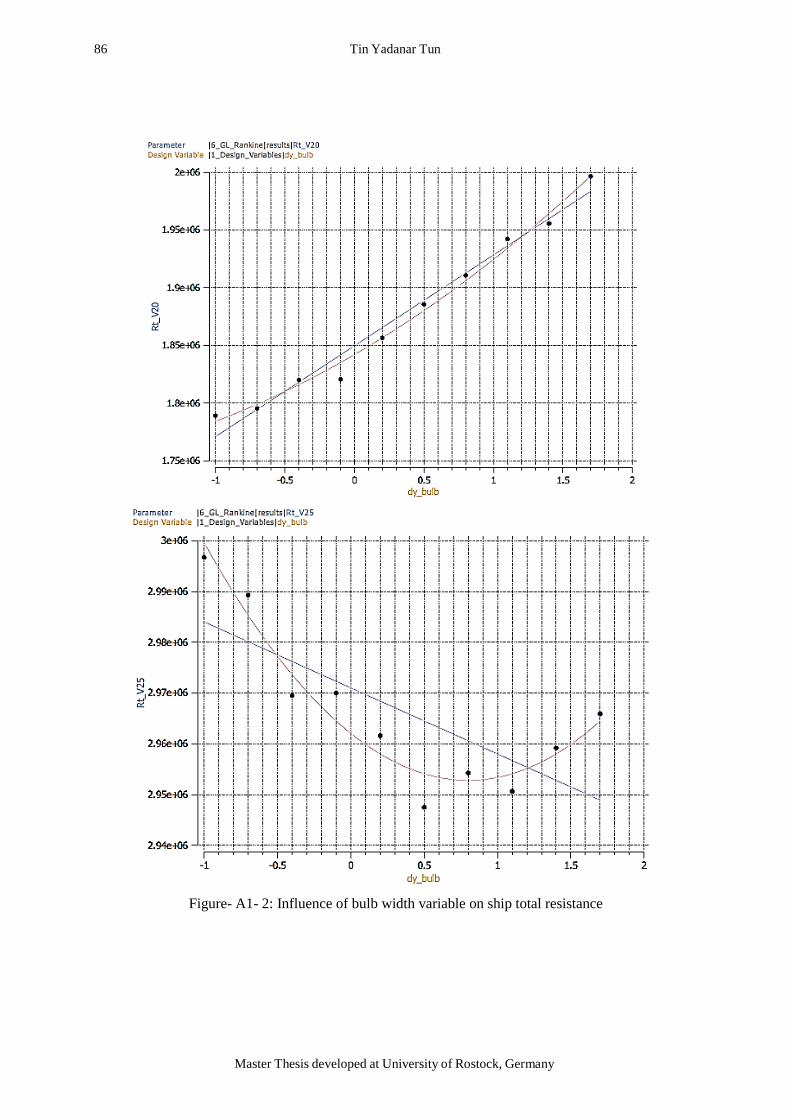
86 Tin Yadanar Tun
Master Thesis developed at University of Rostock, Germany
Figure- A1- 2: Influence of bulb width variable on ship total resistance
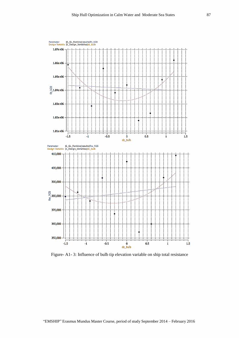
Ship Hull Optimization in Calm Water and Moderate Sea States 87
“EMSHIP” Erasmus Mundus Master Course, period of study September 2014 – February 2016
Figure- A1- 3: Influence of bulb tip elevation variable on ship total resistance

88 Tin Yadanar Tun
Master Thesis developed at University of Rostock, Germany
Figure- A1- 4: Influence of WL entrance angle variable on ship total resistance

Ship Hull Optimization in Calm Water and Moderate Sea States 89
“EMSHIP” Erasmus Mundus Master Course, period of study September 2014 – February 2016
Figure- A1- 5: Influence of Bulb top tangent at FP variable on ship total resistance

90 Tin Yadanar Tun
Master Thesis developed at University of Rostock, Germany
A2. Set-up Input XML File for GL Rankine Solver
A2.1. Sample XML file for Steady Flow Computation
<GLRankine>
<Project version="1.0">
<Configuration>
<ProjectInfo>
<Generator> <Name value="created by Tin"/>
<Version value="1.0"/>
</Generator>
<CreationTime timeStamp=""/>
<CreatedBy name="Tin"/>
<ProjectName value="DTC"/>
</ProjectInfo>
<Computations>
<Preprocessing>
<Bodies>
<Body>
<BodyDefinition name="dtc" sym="1">
<BodyParts>
<BodyPart name="part">
<Surface>
<ReadFromFile type="stl" fileName="DTC.stl"/>
<Transformations>
<Translation dx="0" dy="0" dz="-14.5" />
</Transformations>
<! -- <LimitPlane nx="0" ny="1" nz="0" d="0" /> -->
<WriteToFile type="vtk" fileName="surf.vtk" />
</Surface>
<BodyPanelGeneration>
<double name="lMid" value="3.5"/>
<double name="lBow" value="2.5"/>
<double name="lAft" value="2.5"/>
<double name="zBow" value="1.62008"/>
<double name="zAft" value="0.972048"/>
</BodyPanelGeneration>
</BodyPart>
</BodyParts>
<Transformations>
</Transformations>
<WriteToFile type="vtk" fileName="panels.vtk"/>
<WriteToFile type="shr2" fileName="body-def2.shr2"/>
</BodyDefinition>

Ship Hull Optimization in Calm Water and Moderate Sea States 91
“EMSHIP” Erasmus Mundus Master Course, period of study September 2014 – February 2016
</Body>
</Bodies>
<FreeSurface>
<SetDefaultParameterFor u0="7.9732" />
<FreeSurfaceDefinition>
<RectangularFreeSurface>
</RectangularFreeSurface>
<WriteToFile type="vtk" fileName="fs.vtk"/>
</FreeSurfaceDefinition>
</FreeSurface>
</Preprocessing>
<NonlinearSteadySimulation>
<Data>
<BodyData bodyName="dtc">
<double name="cogZ" value="8.46951" />
</BodyData>
</Data>
<Parameter>
<double name="u0" value="7.9732” />
<double name="rho" value="1025” />
<double name="g" value="9.81” />
<double name="relax” value="0.3”/>
<double name="relax0" value="1”/>
<double name="wdp" value="0.001" />
<unsignedInt name="maxIter" value="100" />
</Parameter>
<Output>
<ResultFile>dump.shr2</ResultFile>
<LogFile>log.out</LogFile>
<VTKDirectory>data</VTKDirectory>
</Output></NonlinearSteadySimulation>
</Computations>
</Configuration>
</Project>
</GLRankine>

92 Tin Yadanar Tun
Master Thesis developed at University of Rostock, Germany
A2.2. Sample XML file for Seakeeping Computation
<? Xml version="1.0" encoding="UTF-8"?>
<GLRankine xmlns: xsi: xsi="http://www.w3.org/2001/XMLSchema-instance"
schemaVersion="1.0" xsi:
noNamespaceSchemaLocation="RankineConfig.xsd">
<Project version="1.0">
<Configuration>
<ProjectInfo>
<Generator>
<Name value="Manually created by Tin"/>
<Version value="1.0"/>
</Generator>
<CreationTime timeStamp="2009-09-29T13:00:59.99Z"/>
<CreatedBy name="Tin"/>
<ProjectName value="PerSee"/>
</ProjectInfo>
<Computations>
<SeakeepingLinear>
<Input>
<StationarySolution>dump.shr2</StationarySolution>
</Input>
<Data>
<BodyData bodyName="dtc">
<double name="GM" value="1.37" />
<double name="rollDamp" value="3" /> <! -- 3% -->
<double name="r_xx" value="20.25" />
<double name="r_yy" value="88.19" />
<double name="r_zz" value="88.49" />
<double name="r2_xy" value="0" />
<double name="r2_xz" value="0" />
<double name="r2_yz" value="0" />
</BodyData>

Ship Hull Optimization in Calm Water and Moderate Sea States 93
“EMSHIP” Erasmus Mundus Master Course, period of study September 2014 – February 2016
<WaveData>
<Waves omega="0.257" muList="180" />
<Waves omega="0.303" muList="180" />
<Waves omega="0.344" muList="180" />
<Waves omega="0.371" muList="180" />
<Waves omega="0.389" muList="180" />
<Waves omega="0.407" muList="180" />
<Waves omega="0.426" muList="180" />
<Waves omega="0.454" muList="180" />
<Waves omega="0.525" muList="180" />
<Waves omega="0.613" muList="180" />
<Waves omega="0.678" muList="180" />
<Waves omega="0.768" muList="180" />
<Waves omega="0.867" muList="180" />
</WaveData>
</Data>
<FreeSurfaceGeneration>
<DefaultGeneration>
<double name="fsGridResolution" value="1.0" />
<double name="fsGridSize" value="1.0" />
</DefaultGeneration>
</FreeSurfaceGeneration>
<Parameter></Parameter>
<Output>
<ResultFile>tf_wo_v16kn.shr2</ResultFile>
<LogFile>log.out</LogFile>
</Output>
</SeakeepingLinear>
</Computations>
</Configuration>
</Project>
</GLRankine>
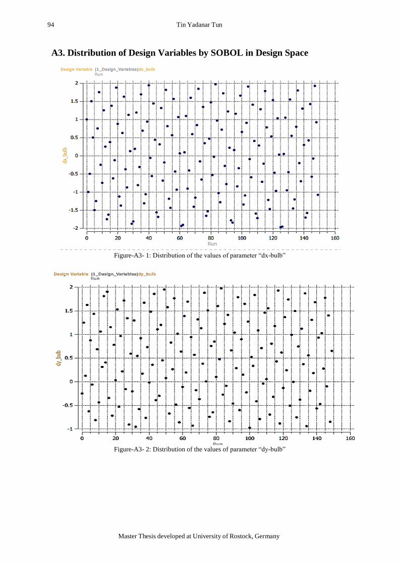
94 Tin Yadanar Tun
Master Thesis developed at University of Rostock, Germany
A3. Distribution of Design Variables by SOBOL in Design Space
Figure-A3- 1: Distribution of the values of parameter “dx-bulb”
Figure-A3- 2: Distribution of the values of parameter “dy-bulb”
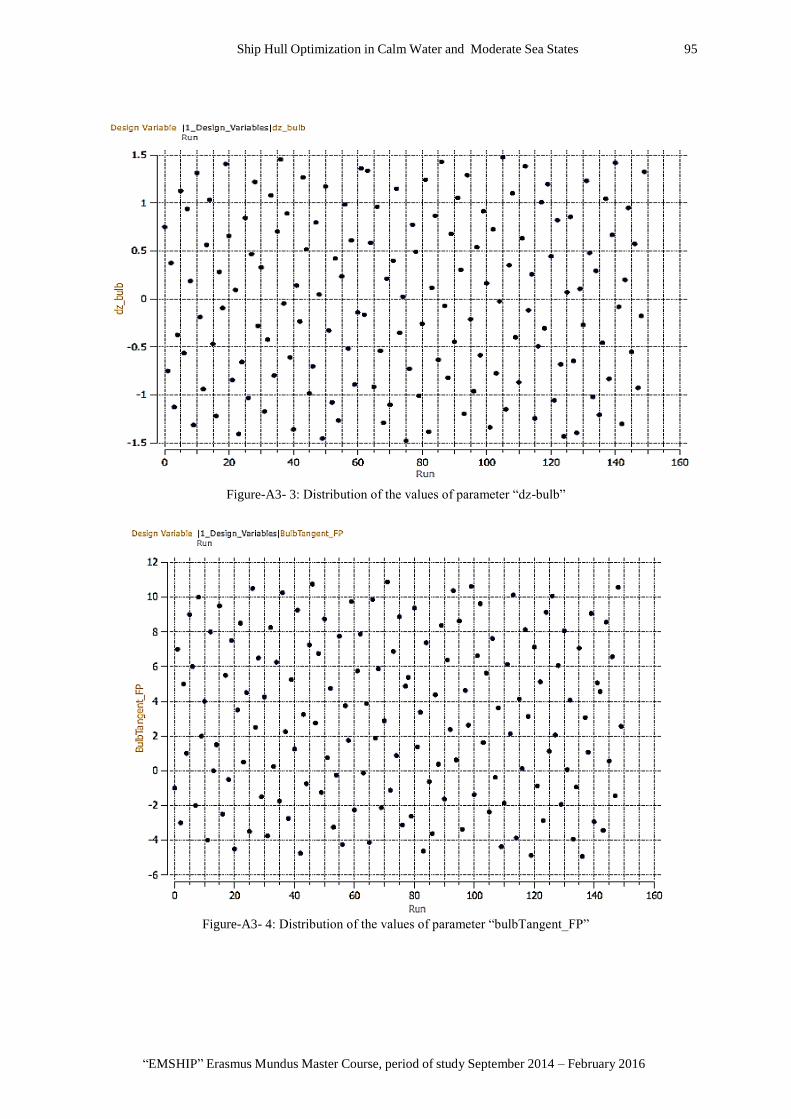
Ship Hull Optimization in Calm Water and Moderate Sea States 95
“EMSHIP” Erasmus Mundus Master Course, period of study September 2014 – February 2016
Figure-A3- 3: Distribution of the values of parameter “dz-bulb”
Figure-A3- 4: Distribution of the values of parameter “bulbTangent_FP”
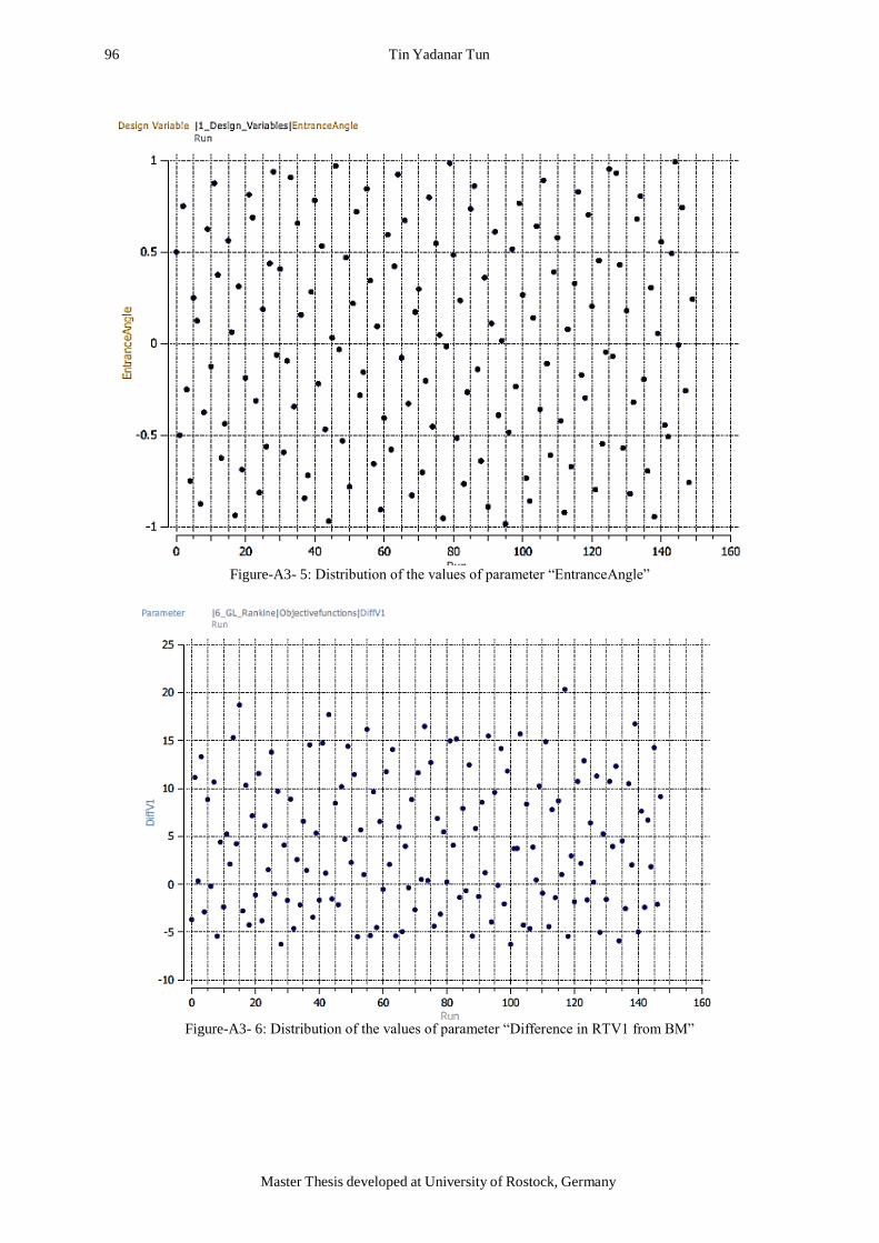
96 Tin Yadanar Tun
Master Thesis developed at University of Rostock, Germany
Figure-A3- 5: Distribution of the values of parameter “EntranceAngle”
Figure-A3- 6: Distribution of the values of parameter “Difference in RTV1 from BM”

Ship Hull Optimization in Calm Water and Moderate Sea States 97
“EMSHIP” Erasmus Mundus Master Course, period of study September 2014 – February 2016
Figure-A3- 7: Distribution of the values of parameter “Difference in RTV2 from BM”
Figure-A3- 8: Distribution of the values of parameter “RTV1”

98 Tin Yadanar Tun
Master Thesis developed at University of Rostock, Germany
Figure-A3- 9: Distribution of the values of parameter “RTV2”
Figure-A3- 10: Distribution of total resistance with weight coefficient= 0.25

Ship Hull Optimization in Calm Water and Moderate Sea States 99
“EMSHIP” Erasmus Mundus Master Course, period of study September 2014 – February 2016
Figure-A3- 11: Distribution of total resistance with weight coefficient= 0.50
Figure-A3- 12: Distribution of total resistance with weight coefficient= 0.75

100 Tin Yadanar Tun
Master Thesis developed at University of Rostock, Germany
A4. Standard Template for Surrogate Based Global Optimization
(CAESES)
environment tabular_graphics_data method_pointer = 'SBGO'
Method
id_method = 'SBGO' surrogate_based_global model_pointer = 'SURROGATE'
approx_method_pointer = 'MOGA' replace_points
max_iterations = 300
Method
id_method = 'MOGA' moga
output silent
seed = 12345
population_size = 300
max_function_evaluations = 5000 initialization_type unique_random crossover_type shuffle_random
num_offspring = 2 num_parents = 2
crossover_rate = 0.8 mutation_type replace_uniform mutation_rate = 0.08 fitness_type
domination_count
replacement_type below_limit = 6 shrinkage_percentage = 0.9 convergence_type metric_tracker
percent_change = 0.1
num_generations = 30
final_solutions = 10
model
id_model = 'SURROGATE' surrogate global gaussian_process surfpack trend constant
dace_method_pointer = 'SAMPLING' correction additive zeroth_order
reuse_points all import_points_file = 'model.dat'
method
id_method = 'SAMPLING' model_pointer = 'TRUTH' sampling
samples = 50
seed = 54321 sample_type lhs
model
id_model = 'TRUTH' single
variables continuous_design = 5
initial_point 0 0 0 0 0
lower_bounds -2 -1 -1.5 -5 -1
upper_bounds 2 2 1.5 11 1
descriptors ‘|1_Design_Variables|dx_bulb' '|1_Design_Variables|dy_bulb'
'|1_Design_Variables|dz_bulb' '|1_Design_Variables|BulbTangent_FP'
'|1_Design_Variables|EntranceAngle'
responses objective_functions = 2
nonlinear_inequality_constraints = 0
nonlinear_equality_constraints = 0 no_gradients
no_hessians
interface fork
analysis_driver = 'fdakota_client.exe' verbatim parameters_file = 'params.in' results_file =
'results.out' work_directory directory_tag
named 'design' file_save directory_save
asynchronous evaluation_concurrency = 24

Ship Hull Optimization in Calm Water and Moderate Sea States
“EMSHIP” Erasmus Mundus Master Course, period of study September 2014 – February 2016
101
A5. MATLAB Code for Calculating the Added Wave Resistance
% define Pierson-Moskowitz (ITTC) spectrum parameters
T = 0.5:1:20.5;
w1= [0.1;0.2;0.3;0.4;0.5;0.6;0.7;0.8;0.9;1.0;1.1];
Hs = 0.75:0.5:3.25;
load results.mat; % results obtained from the GLRankine seakeeping computations
Fx_180= zeros (length (w1), 1);
Fx_150= zeros (length (w1), 1);
Fx_120= zeros (length (w1), 1);
count =1;
for i=1: length (w1)
Fx_180 (i) = -1*Results (count, 3);
Fx_150 (i) = -1*Results (count+1, 3);
Fx_120 (i) = -1*Results (count+2, 3);
count=count+3;
end
Raw1_180 (length (Hs), length (T)) =zeros ();
Radd_max_180 (length (Hs), 1) =zeros ();
Tp_180 (length (Hs), 1) =zeros ();
Raw1_150 (length (Hs), length (T)) =zeros (); Radd_max_150 (length (Hs), 1) =zeros ();
Tp_150 (length (Hs), 1) =zeros ();
Raw1_120 (length (Hs), length (T)) =zeros (); Radd_max_120 (length (Hs), 1) =zeros ();
Tp_120 (length (Hs), 1) =zeros ();
for k= 1: length (Hs)
Raw_180= zeros (size (T));
Raw_150= zeros (size (T));
Raw_120= zeros (size (T));
for j= 1: length (T)
S1= zeros (size (w1));
for i= 1: length (w1)
Af= 173*Hs (k) ^2/T (j) ^4;
Bf= 691/T (j) ^4;

Master Thesis developed at University of Rostock, Germany
102 Tin Yadanar Tun
S1 (i) = Af*w1 (i) ^-5*exp (-1*Bf*w1 (i) ^-4);
end
RAW_180 =S1.* Fx_180;
Raw_180 (j) = 2*trapz (w1, RAW_180);
If (j>1)
if (Raw_180 (j)>Raw_180 (j-1))
Radd_max_180 (k, 1) =Raw_180 (j); Tp_180
(k, 1) = T (j);
end
end
RAW_150 =S1.* Fx_150;
Raw_150 (j) = 2*trapz (w1,RAW_150);
if (j>1)
if (Raw_150(j)>Raw_150(j-1))
Radd_max_150(k,1)=Raw_150(j);
Tp_150(k,1)= T(j);
end
end
RAW_120 =S1.* Fx_120;
Raw_120(j) = 2*trapz(w1,RAW_120);
if (j>1)
if (Raw_120(j)>Raw_120(j-1))
Radd_max_120(k,1)=Raw_120(j);
Tp_120(k,1)= T(j);
end
end
end
Raw1_180 (k,:)= Raw_180/Rtcalmwater*100;
Raw1_150 (k,:)= Raw_150/Rtcalmwater*100;
Raw1_120 (k,:)= Raw_120/Rtcalmwater*100;
end