Ship Detection and Property Extraction in Radar Images on Hardware

by

Koray Kilinc

B.Sc., Bilkent University, 2013

A Thesis Submitted in Partial Fulfillment of the

Requirements for the Degree of

Master of Applied Science

in the Department of Electrical and Computer Engineering

© Koray Kilinc, 2015

University of Victoria

All rights reserved. This thesis may not be reproduced in whole or in part, by

photocopying or other means, without the permission of the author.

ii

Ship Detection and Property Extraction in Radar Images on Hardware

by

Koray Kilinc

B.Sc., Bilkent University, 2013

Supervisory Committee

Dr. Fayez Gebali, Supervisor

(Department of Electrical and Computer Engineering)

Dr. Kin Fun Li, Co-Supervisor

(Department of Electrical and Computer Engineering)

Dr. Caterina Valeo, Outside Member

(Department of Mechanical Engineering)

iii

Supervisory Committee

Dr. Fayez Gebali, Supervisor

(Department of Electrical and Computer Engineering)

Dr. Kin Fun Li, Co-Supervisor

(Department of Electrical and Computer Engineering)

Dr. Caterina Valeo, Outside Member

(Department of Mechanical Engineering)

ABSTRACT

In this work we review the problem of radar imaging satellites’ dependency on

ground stations to transfer the image data. Since synthetic aperture radar images

are very big, only ground stations are equipped to transfer that much data. This

is a problem for maritime surveillance as it creates delay between the imaging and

processing. We propose a new hardware algorithm that can be used by a satellite to

detect ships and extract information about them, and since this information is smaller

it can be relayed to reduce the delay significantly. For ship detection, an adaptive

thresholding algorithm with exponential model is used. This algorithm was selected

as it is the best fit for single-look radar images. For the property calculation, a data

accumulating, single-look, connected component labeling algorithm is proposed. This

algorithm accumulates data about the connected components, which is then used to

calculate the properties of ships using image moments. The combined algorithm was

then validated on Radarsat-2 images using Matlab for software and co-simulation for

hardware.

iv

Contents

Supervisory Committee ii

Abstract iii

Table of Contents iv

List of Tables vii

List of Figures viii

Acknowledgements x

1 Introduction 1

1.1 Overview . . . . . . . . . . . . . . . . . . . . . . . . . . . . . . . . . . 1

1.2 Motivation for this work . . . . . . . . . . . . . . . . . . . . . . . . . 2

1.3 Contributions . . . . . . . . . . . . . . . . . . . . . . . . . . . . . . . 3

1.4 Thesis Organization . . . . . . . . . . . . . . . . . . . . . . . . . . . . 3

2 Ship Detection and Property Calculation 5

2.1 Ship Detection . . . . . . . . . . . . . . . . . . . . . . . . . . . . . . 6

2.1.1 Ship Wake Analysis . . . . . . . . . . . . . . . . . . . . . . . . 7

2.1.2 Global Threshold and Morphology . . . . . . . . . . . . . . . 9

2.1.3 Adaptive Threshold . . . . . . . . . . . . . . . . . . . . . . . . 10

2.2 Property Calculation . . . . . . . . . . . . . . . . . . . . . . . . . . . 12

2.2.1 Connected Component Labeling . . . . . . . . . . . . . . . . . 12

2.2.2 Image Moments . . . . . . . . . . . . . . . . . . . . . . . . . . 14

2.3 Chapter Summary . . . . . . . . . . . . . . . . . . . . . . . . . . . . 15

3 Proposed Algorithm for Detection and Characterization of Ships

in SAR Images 16

v

3.1 Reason for considerations . . . . . . . . . . . . . . . . . . . . . . . . . 16

3.2 Proposed Algorithm . . . . . . . . . . . . . . . . . . . . . . . . . . . 17

3.2.1 Thresholding . . . . . . . . . . . . . . . . . . . . . . . . . . . 18

3.2.2 Clustering and Data Accumulation . . . . . . . . . . . . . . . 20

3.2.3 Calculation of Ship Parameters . . . . . . . . . . . . . . . . . 24

3.3 Chapter Summary . . . . . . . . . . . . . . . . . . . . . . . . . . . . 25

4 Implementation 26

4.1 Software Implementation . . . . . . . . . . . . . . . . . . . . . . . . . 26

4.2 Hardware Implementation . . . . . . . . . . . . . . . . . . . . . . . . 26

4.2.1 Thresholding . . . . . . . . . . . . . . . . . . . . . . . . . . . 30

4.2.2 Data Accumulation . . . . . . . . . . . . . . . . . . . . . . . . 31

4.2.3 Property Calculation . . . . . . . . . . . . . . . . . . . . . . . 33

4.2.4 Storage . . . . . . . . . . . . . . . . . . . . . . . . . . . . . . 34

4.3 Chapter Summary . . . . . . . . . . . . . . . . . . . . . . . . . . . . 34

5 Experimental Work 36

5.1 Setup . . . . . . . . . . . . . . . . . . . . . . . . . . . . . . . . . . . . 36

5.1.1 Experiment 1: Ship Detection on a low resolution SAR image

using software . . . . . . . . . . . . . . . . . . . . . . . . . . . 36

5.1.2 Experiment 2: Ship Detection on a low resolution SAR image

using hardware . . . . . . . . . . . . . . . . . . . . . . . . . . 37

5.1.3 Experiment 3: Ship Detection on a high resolution SAR image

using hardware . . . . . . . . . . . . . . . . . . . . . . . . . . 37

5.2 Analysis . . . . . . . . . . . . . . . . . . . . . . . . . . . . . . . . . . 37

5.2.1 Experiment 1 Analysis . . . . . . . . . . . . . . . . . . . . . . 37

5.2.2 Experiment 2 Analysis . . . . . . . . . . . . . . . . . . . . . . 39

5.2.3 Experiment 3 Analysis . . . . . . . . . . . . . . . . . . . . . . 40

5.2.4 Timing and Power Results . . . . . . . . . . . . . . . . . . . . 41

5.3 Chapter Summary . . . . . . . . . . . . . . . . . . . . . . . . . . . . 42

6 Conclusion, Contributions and Future Work 43

6.1 Conclusion . . . . . . . . . . . . . . . . . . . . . . . . . . . . . . . . . 43

6.2 Contributions . . . . . . . . . . . . . . . . . . . . . . . . . . . . . . . 44

6.3 Future Work . . . . . . . . . . . . . . . . . . . . . . . . . . . . . . . . 44

6.3.1 Detecting movement of ships . . . . . . . . . . . . . . . . . . . 44

vi

6.3.2 Multi-look images . . . . . . . . . . . . . . . . . . . . . . . . . 44

6.3.3 Land Masking . . . . . . . . . . . . . . . . . . . . . . . . . . . 45

References 46

A Appendix 50

A.1 Matlab Code for Software Implementation . . . . . . . . . . . . . . . 50

vii

List of Tables

Table 2.1 RADARSAT-2 modes with their respective resolution and nomi-

nal scene sizes . . . . . . . . . . . . . . . . . . . . . . . . . . . . 5

Table 4.1 Port specifications of top level . . . . . . . . . . . . . . . . . . . 29

Table 4.2 Port specifications of thresholding subsystem . . . . . . . . . . . 31

Table 4.3 Port specifications of data accumulation subsystem . . . . . . . 33

Table 4.4 Port specifications of property calculation subsystem . . . . . . 34

Table 4.5 Port specifications of storage subsystem . . . . . . . . . . . . . . 35

Table 5.1 Detection of pixel targets on RADARSAT-2 images . . . . . . . 38

Table 5.2 Detection of targets on RADARSAT-2 images on software . . . 39

Table 5.3 Utilization of the algorithm on hardware . . . . . . . . . . . . . 39

Table 5.4 Detection of targets on RADARSAT-2 images on hardware . . . 40

viii

List of Figures

Figure 1.1 Moving of the SAR antenna . . . . . . . . . . . . . . . . . . . . 2

Figure 1.2 Illustration of the SAR process . . . . . . . . . . . . . . . . . . 2

Figure 2.1 Three types of reflection seen in radar imaging: (a) specular

reflection, (b) diffused reflection, (c) corner reflection . . . . . . 7

Figure 2.2 SAR image of an ocean . . . . . . . . . . . . . . . . . . . . . . 7

Figure 2.3 Components of ship wakes [8] . . . . . . . . . . . . . . . . . . . 8

Figure 2.4 Ship wake in a SAR image . . . . . . . . . . . . . . . . . . . . . 9

Figure 2.5 Illustration of nested windows . . . . . . . . . . . . . . . . . . . 10

Figure 2.6 First pass 3x3 window for multi-pass algorithm [21] . . . . . . . 12

Figure 2.7 Mask: Mask: Pixels in the neighbourhood of X . . . . . . . . . 13

Figure 2.8 Image ellipse with properties . . . . . . . . . . . . . . . . . . . 15

Figure 3.1 Block diagram for the proposed algorithm . . . . . . . . . . . . 17

Figure 3.2 Frames of the SAR image . . . . . . . . . . . . . . . . . . . . . 18

Figure 3.3 Nested windows: (a) 2D nested windows, (b) 1D nested windows 19

Figure 3.4 Thresholding: (a) Original image, (b) binary image after thresh-

olding . . . . . . . . . . . . . . . . . . . . . . . . . . . . . . . . 20

Figure 3.5 Flowchart for labeling . . . . . . . . . . . . . . . . . . . . . . . 21

Figure 3.6 Labeling: (a) Binary image, (b) after labeling each color repre-

sents a different label . . . . . . . . . . . . . . . . . . . . . . . . 22

Figure 3.7 Flowchart for merging . . . . . . . . . . . . . . . . . . . . . . . 23

Figure 3.8 Merging: (a) Initial labeling where each line has different label,

(b) after merging the adjacent lines get the same label . . . . . 23

Figure 4.1 Flowchart for software implementation . . . . . . . . . . . . . . 27

Figure 4.2 Example block diagram using System Generator . . . . . . . . . 28

Figure 4.3 Top level of hardware implementation . . . . . . . . . . . . . . 28

Figure 4.4 Connections of subsystems . . . . . . . . . . . . . . . . . . . . . 29

ix

Figure 4.5 Structure of thresholding algorithm . . . . . . . . . . . . . . . . 30

Figure 4.6 Thresholding subsystem . . . . . . . . . . . . . . . . . . . . . . 31

Figure 4.7 Data accumulation subsystem . . . . . . . . . . . . . . . . . . . 31

Figure 4.8 Property calculation subsystem . . . . . . . . . . . . . . . . . . 33

Figure 4.9 Storage subsystem . . . . . . . . . . . . . . . . . . . . . . . . . 35

Figure 5.1 A 250x250 SAR image with 25m resolution . . . . . . . . . . . 38

Figure 5.2 Results of the algorithm: (a) is the original image, (b) is the ship

detected image, (c) is the original image with bounding boxes

around detected ships . . . . . . . . . . . . . . . . . . . . . . . 41

Figure 5.3 (a) Timing results, (b) Power Results . . . . . . . . . . . . . . . 42

x

ACKNOWLEDGEMENTS

I would like to thank:

My mother Serap Kilinc and my father Ilhami Kilinc, for their prayers, love,

patience, emotional support, motivation and assurance in diffcult and frustrat-

ing moments and for their constant motivation.

My supervisors Dr. Fayez Gebali and Dr. Kin Fun Li, for all the mentoring

and support which enabled me to achieve my academic and research objectives.

Chapter 1

Introduction

1.1 Overview

Imaging radars form image of a target area by sending electromagnetic pulses and reg-

istering the intensity of the reflected echo to determine the amount of scattering. The

registered electromagnetic scattering is then mapped onto a two-dimensional plane,

with points of a higher reflectivity getting assigned a brighter color, thus creating an

image. Synthetic aperture radar (SAR) builds on the same idea but uses the mo-

tion of the SAR antenna over a target region to provide finer spatial resolution than

is possible with conventional beam-scanning radars. The distance the SAR device

travels over a target creates a large “synthetic” antenna aperture (the “size” of the

antenna).

To create a SAR image, successive pulses of radio waves are transmitted to “il-

luminate” a target scene, and the echo of each pulse is received and recorded. The

pulses are transmitted and the echoes received using a single beam-forming antenna.

As shown in Figure 1.1, as the SAR device on board the aircraft or spacecraft moves,

the antenna location relative to the target changes over time. Signal processing of the

recorded radar echoes combines the recordings from the multiple antenna locations.

This forms the synthetic antenna aperture, and allows it to create finer resolution

image than what would be possible with the given physical antenna aperture [1].

SAR images have various applications such as: surface topography, storm moni-

toring, maritime surveillance. Figure 1.2 shows the steps of image creation with the

added step of image parsing. Image parsing is used to extract information from the

images depending on the application.

2

Figure 1.1: Moving of the SAR antenna

Figure 1.2: Illustration of the SAR process

1.2 Motivation for this work

Due to the large data size of the radar images, the satellites need to transfer the

image to nearby ground stations, which are equipped to handle large data transfers.

However since satellites follow a set orbit, they need to wait until they are close to a

ground station before they can send the data, this causes orbit delay. The other three

causes of delay are signal processing delay, which is caused while forming the image;

transmission delay, caused while transferring the data to the ground, and parsing

delay, which is caused while extracting information from the images.

Maritime surveillance is the task of monitoring areas of water. Radar images

are used to detect human activities, in particular ship detection, for interdiction of

criminal activities and for ensuring legal use of waters. For quicker response, the delay

between the acquisition of the image and detection of the threat should be minimized.

Since the major contributor to the response time is the orbit delay, this research

focuses on reducing this delay.

3

One approach is to create more ground stations to cover more of the satellites

orbit path. However this requires money, land and manpower. Another approach is

to reduce the data size so that the satellite doesn’t depend on the ground station.

In radar images taken for maritime surveillance, the targets of interest, ships, only

take up a small portion of the whole image where the ocean takes up the rest. Thus,

another approach is to extract information about ships on the satellite to reduce the

data size.

In this thesis, it is proposed that the image is processed directly on the satellite

to detect and characterize ships. This approach decreases the size of the data to be

transferred, and since the data is relatively small, the data can be relayed through

ships and planes, thus reducing the delay and allowing for quicker response.

The implementation of the processing can be done in two ways: software and

hardware. Both allow parallel computing but hardware enables an application specific

design which allows for a faster, robust system with low power cost.

1.3 Contributions

The following contributions are made in this work:

� Development of an algorithm that can detect ships in radar images

� Development of an algorithm that can calculate the location, size and orienta-

tion properties of connected components (ships)

� Evaluation of the software and hardware implementations of the above algo-

rithms

This work lowers the response time in maritime surveillance by reducing the data

size to only the information about the detected ships and thus, eliminating the need

for a ground station.

1.4 Thesis Organization

This section outlines the organization of the thesis and provides a brief summary of

the main focus for each chapter.

4

Chapter 1 introduces the reader to the subject and the scope of the research. The

motivation and the contributions of the research are discussed, which are the

fundamental objectives of this thesis.

Chapter 2 describes the background and fundamentals of ship detection. A brief

analysis of ship detection and property calculation methods are provided in

order to aid the reader in understanding related previous work done in the

area.

Chapter 3 describes our approach towards the extraction of ship properties from

radar images. The chosen ship detection algorithm, adaptive thresholding, as

well as the new proposed method for property extraction, are presented and

their methodology explained.

Chapter 4 describes the software/hardware design and implementation. The system

hardware subsystems are further explained.

Chapter 5 contains the experimental setup and analysis. The simulation results of

software and hardware are obtained to verify that the algorithms work correctly

and then the performance analysis of the hardware is conducted.

Chapter 6 has the concluding statements and a short description of the research

work and what have been achieved through this work.

5

Chapter 2

Ship Detection and Property

Calculation

Satellite imagery has always been a focus of interest for governments and businesses

around the world. Even though earlier applications were limited and relied on optical

imaging, with the advance in technology, radar imaging has become more popular as

it provides more information about the target area and is not affected by the weather.

Synthetic Aperture Radar (SAR) creates a synthetic aperture, which allows it to have

high resolution images without the need of a long antenna. Jackson et al. [2] explains

how SAR works in more detail. SAR uses the object reflectivity, quantized by radar

cross section (RCS), to form images.

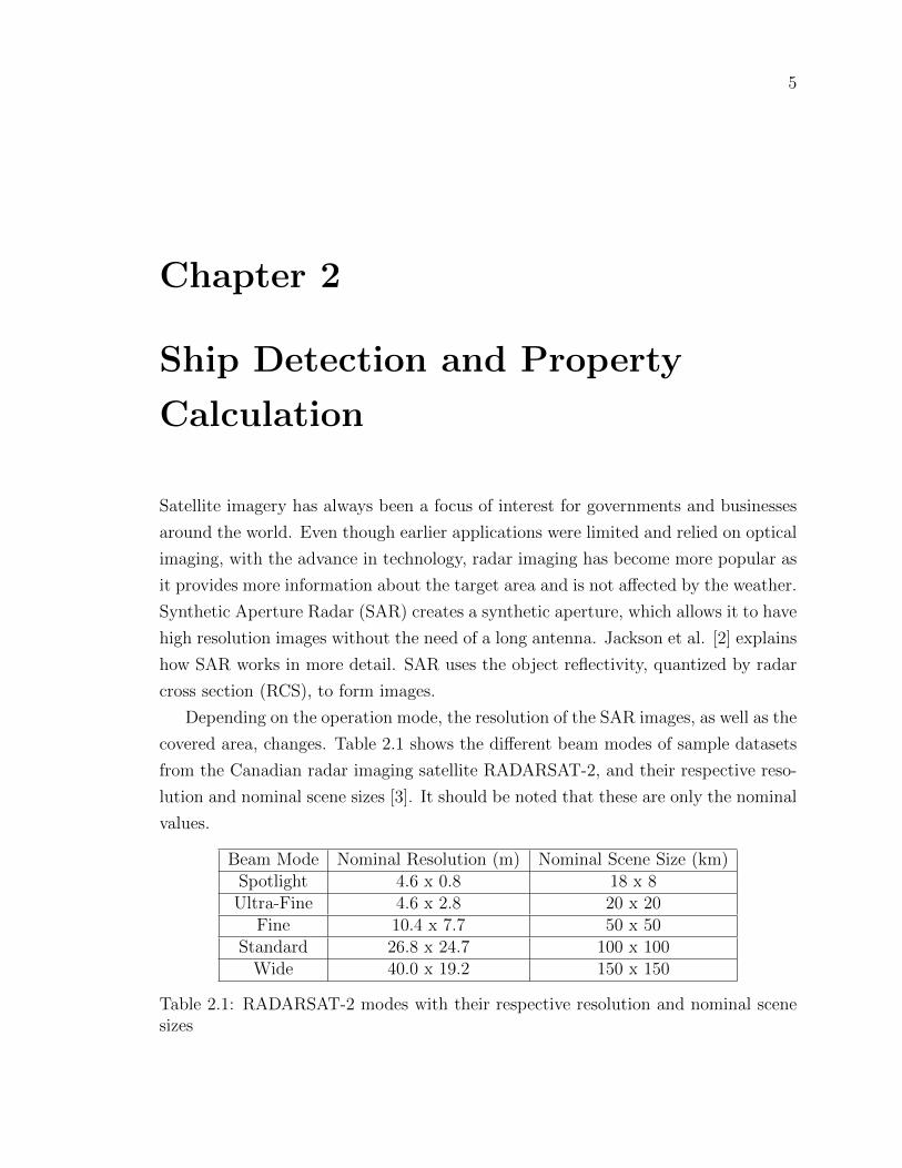
Depending on the operation mode, the resolution of the SAR images, as well as the

covered area, changes. Table 2.1 shows the different beam modes of sample datasets

from the Canadian radar imaging satellite RADARSAT-2, and their respective reso-

lution and nominal scene sizes [3]. It should be noted that these are only the nominal

values.

Beam Mode Nominal Resolution (m) Nominal Scene Size (km)Spotlight 4.6 x 0.8 18 x 8

Ultra-Fine 4.6 x 2.8 20 x 20Fine 10.4 x 7.7 50 x 50

Standard 26.8 x 24.7 100 x 100Wide 40.0 x 19.2 150 x 150

Table 2.1: RADARSAT-2 modes with their respective resolution and nominal scenesizes

6

As the SAR imagery spans hundreds of kilometers, the data size becomes very big.

This causes the satellite to only be able to downlink the data to a ground station,

which can handle the transfer of a large volume of data in a short time. This means

the data won’t be processed until the satellite passes over a ground station. This

creates a delay between the time when the image is taken and the time when the

image is processed.

SAR data has many applications such as:

� Conducting maritime surveillance (e.g., ship detection);

� Monitoring/tracking ice;

� Detecting oil spills;

� Monitoring floods, landslides, eruptions;

� Aiding forest firefighting.

In the ship detection part of maritime surveillance, the focus is on the ships

instead of the ocean, which is only a small percentage of the whole image. Thus, if

the information about the ships can be extracted from the image directly, it would be

possible to relay the relatively small data without the use of ground stations which

would reduce the delay and allow for a quicker response if necessary. The available

ship detection and property calculation algorithms are given below.

2.1 Ship Detection

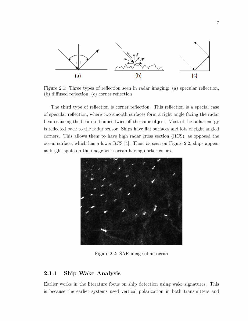
As SAR uses radar reflectivity to create images, analyzing the effects of different

reflection types would give an insight on how the images are created. The three types

of reflection seen in radar imaging are illustrated in Figure 2.1. These reflections are:

specular, diffused and corner reflection. In specular reflection, the smooth surface

acts like a mirror for the incident radar pulse. Most of the incident radar energy is

reflected away according to the law of specular reflection, i.e., the angle of reflection

is equal to the angle of incidence. Very little energy is scattered back to the radar

sensor. However, in diffused reflection, the rough surface reflects the incident radar

pulse in all directions. Part of the radar energy is scattered back to the radar sensor.

The amount of energy backscattered depends on the properties of the target on the

ground.

7

Figure 2.1: Three types of reflection seen in radar imaging: (a) specular reflection,(b) diffused reflection, (c) corner reflection

The third type of reflection is corner reflection. This reflection is a special case

of specular reflection, where two smooth surfaces form a right angle facing the radar

beam causing the beam to bounce twice off the same object. Most of the radar energy

is reflected back to the radar sensor. Ships have flat surfaces and lots of right angled

corners. This allows them to have high radar cross section (RCS), as opposed the

ocean surface, which has a lower RCS [4]. Thus, as seen on Figure 2.2, ships appear

as bright spots on the image with ocean having darker colors.

Figure 2.2: SAR image of an ocean

2.1.1 Ship Wake Analysis

Earlier works in the literature focus on ship detection using wake signatures. This

is because the earlier systems used vertical polarization in both transmitters and

8

receivers resulting in large and distinct wake signatures [5, 6]. Figure 2.3 shows

the different components of a ship wake. By processing the image to detect these

components, ships can be detected. The wakes can also be further analyzed to extract

more information such as the beam and speed of ships [7].

Figure 2.3: Components of ship wakes [8]

Depending on the configuration of the SAR system, one or more of the following

features, as shown in Figure 2.4, are visible. First, the wake is nearly always charac-

terized by a dark trail which is caused by the turbulent vortex created by the ship.

Turbulent vortex reduces the roughness of the sea which causes a lower RCS. The

dark wake may be delimited by one or two bright lines. Sometimes also, another

set of bright arms can be visible: they are located at the border of the Kelvin wave

system and form a characteristic angle of about 39◦.

Ship detection algorithms using wakes can be advantageous as the wakes are more

noticeable, which can help if the ship is in a high clutter area, making the ship

itself harder to detect [9]. However, it is found that ship backscatter is robust and

independent of the sea state whereas wakes are often not visible at large incident

angles and long wavelengths [10]. Because of these reasons, along with the fact that

9

Figure 2.4: Ship wake in a SAR image

stationary and slow moving ships don’t create wakes, the focus of the later literature

moved on to the detection of the ship target itself. Vachon et al. [11] show that by

using horizontal polarization, it is possible to create a better ship-sea contrast making

the ships stand out more in the image.

2.1.2 Global Threshold and Morphology

Since ships appear as bright pixels while the pixels belonging to the ocean are dark,

the first thing comes to mind is finding a threshold value to separate targets from the

background. Lin et al.[12] use an arbitrary global threshold for the entire image, but

use a post-processing of morphological closing. Morphological closing works by first

dilating all the detections which fills small holes inside ship pixel clusters and connects

neighbor ship pixels that belong to the same ship. Dilation operation is followed

by erosion, which eliminates isolated detections. More information about how the

morphological operations work can be found in [13]. Even though this approach can

reduce false detections, it is prone to error if false detections are clustered together

where the dilation operation would fill the gaps between false detections, which would

prevent the closing operation from eliminating these false detections. More so, if a

ship is represented with only one pixel, the closing operation would end up eliminating

the detection causing a missed detection.

10

2.1.3 Adaptive Threshold

Factors like change in incidence angle and different sea states such as height of waves

in the ocean can change the RCS of the ocean as well as of ships. This makes

using a single threshold for the whole image unfeasible and therefore, creates a need

for localized thresholds. One approach is to divide the image into smaller areas

and create individual thresholds for each area. The other approach is to have a

moving window that decides if the pixel is a valid target according to its surroundings

for each pixel. Since the threshold for each pixel depends on the statistics of that

individual pixel’s surroundings, these types of algorithms are called adaptive threshold

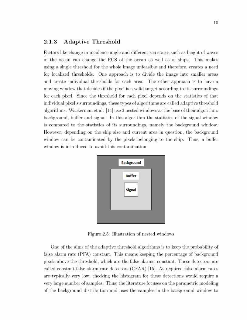
algorithms. Wackerman et al. [14] use 3 nested windows as the base of their algorithm:

background, buffer and signal. In this algorithm the statistics of the signal window

is compared to the statistics of its surroundings, namely the background window.

However, depending on the ship size and current area in question, the background

window can be contaminated by the pixels belonging to the ship. Thus, a buffer

window is introduced to avoid this contamination.

Figure 2.5: Illustration of nested windows

One of the aims of the adaptive threshold algorithms is to keep the probability of

false alarm rate (PFA) constant. This means keeping the percentage of background

pixels above the threshold, which are the false alarms, constant. These detectors are

called constant false alarm rate detectors (CFAR) [15]. As required false alarm rates

are typically very low, checking the histogram for these detections would require a

very large number of samples. Thus, the literature focuses on the parametric modeling

of the background distribution and uses the samples in the background window to

11

estimate the model parameters.

Given the required probability of false alarm rate (PFA) and the parametric prob-

ability density function of the background f(x), the threshold T can be found by

PFA =

∫ ∞T

f(x)dx (2.1)

The thresholding of the tested pixel xt is established simply by comparing it to the

threshold T. If the target pixel has a higher value than the threshold, it is detection.

That means ∫ ∞xt

f(x)dx < PFA (2.2)

Since xt and PFA is already known, all that is required is to find a good model

for the background. One approach is using Gaussian distribution to model the back-

ground. With the Gaussian distribution the detection test becomes

xt > µb + σbt (2.3)

where xt is the tested pixel value, µb is the background mean, σb is the background

standard deviation, and t is a design parameter, which controls the PFA according

to

PFA =1

2− 1

2erf

(t√2

)(2.4)

Another model to consider is the negative exponential, which is used for single-

look SAR images. These images are created by using only one look compared to

multi-look images which create an image by taking several looks at a target in a

single radar sweep and averaging them [16].

By fitting the exponential model into equation 2.2, the resulting detector becomes

xt > µbt (2.5)

where xt is the tested pixel value, µb is the background mean, and t is a design param-

eter. Friedman et al. [17] suggest that to maximize ship detection while minimizing

false detections, t should be selected between 5.5-6.0 for high resolution images and

5.0-5.5 for low resolution images.

There are other models to consider. Wang et al. [18] proposes an alpha-stable

12

distribution, which is widely used for impulsive or spiky signal processing, to describe

the background sea clutter. Another distribution to consider is the k-distribution,

which is prominently used in multi-look radar images [19, 20].

2.2 Property Calculation

2.2.1 Connected Component Labeling

Multi-pass Algorithm

Depending on the resolution of the radar and the ship size, ship may appear as

multiple pixels in the SAR image. Thus, after thresholding, these detections should

be handled as one ship instead of individual ships. Connected component labeling

algorithms can be used to label pixels belonging to each ship.

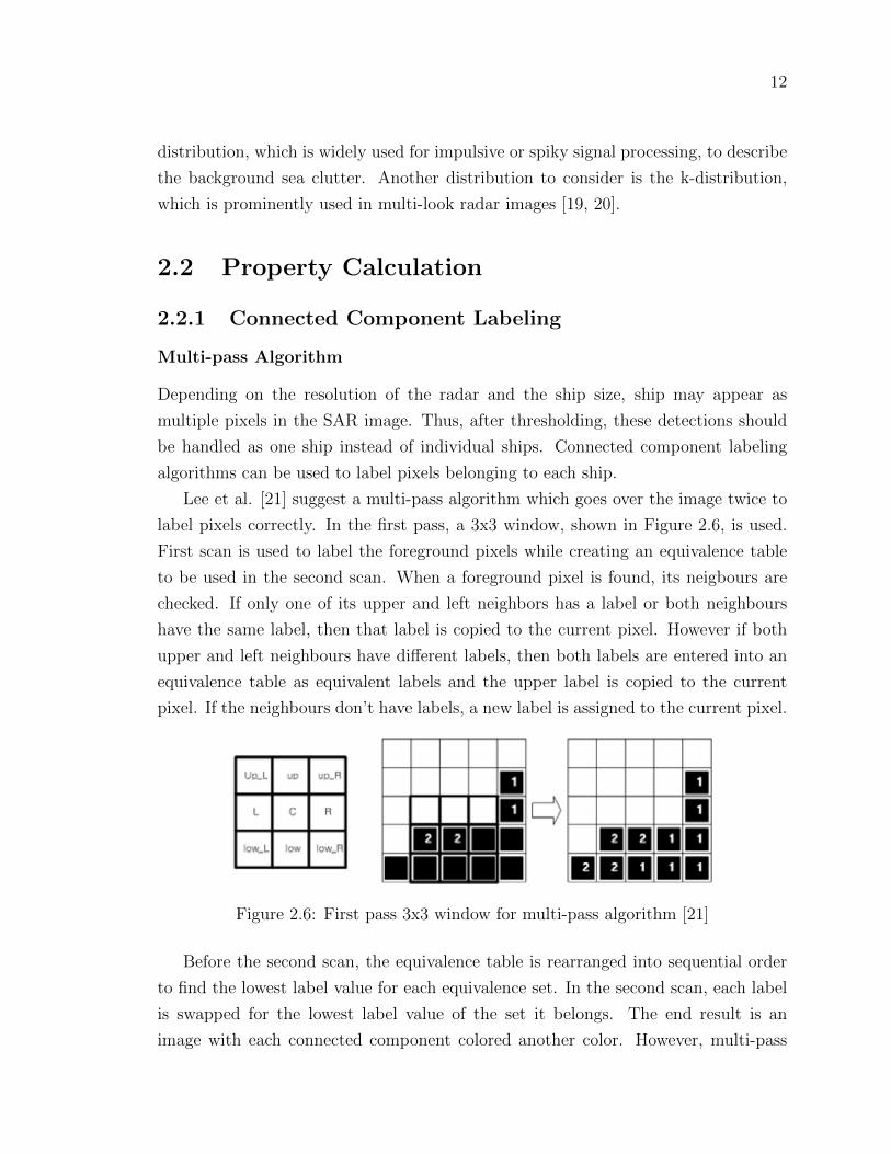
Lee et al. [21] suggest a multi-pass algorithm which goes over the image twice to

label pixels correctly. In the first pass, a 3x3 window, shown in Figure 2.6, is used.

First scan is used to label the foreground pixels while creating an equivalence table

to be used in the second scan. When a foreground pixel is found, its neigbours are

checked. If only one of its upper and left neighbors has a label or both neighbours

have the same label, then that label is copied to the current pixel. However if both

upper and left neighbours have different labels, then both labels are entered into an

equivalence table as equivalent labels and the upper label is copied to the current

pixel. If the neighbours don’t have labels, a new label is assigned to the current pixel.

Figure 2.6: First pass 3x3 window for multi-pass algorithm [21]

Before the second scan, the equivalence table is rearranged into sequential order

to find the lowest label value for each equivalence set. In the second scan, each label

is swapped for the lowest label value of the set it belongs. The end result is an

image with each connected component colored another color. However, multi-pass

13

algorithms are not well suited for streamed images since they require buffering of

intermediate images between passes.

Single-pass Algorithm

Single pass connected component algorithms on hardware focus on the analysis of

the connected components in single pass by gathering data on the regions as they

are built. This avoids the need for buffering the image, making it ideally suited for

processing streamed images on an FPGA.

Figure 2.7: Mask: Mask: Pixels in the neighbourhood of X

Johnston et al. [22] proposes a single pass algorithm to calculate the area of

connected components. This algorithm have the following steps:

1. The neighbourhood mask, shown in Figure 2.7, provides the labels of the four

pixels adjacent to the current pixel. A row buffer caches the labels from the

previous row. These must be looked up in the merger table to correct the label

for any mergers since the pixel was cached.

2. Label selection assigns the label for the current pixel based on the labels of its

neighbours:

� background pixels are labelled 0;

� if all neighbouring labels are background a new label is assigned;

� if only a single label appears among the labelled neighbours, that is se-

lected;

� if the neighbours have two distinct labels, those regions are merged, and

the smaller of the two labels is retained and selected.

3. The merger table is updated when two objects are merged. The larger label is

modified to point to the smaller label used to represent the region.

14

4. The data required to calculate the area of each connected component is accu-

mulated. When regions are merged, the corresponding accumulated data are

also merged.

The disadvantage of single pass algorithms is that the information about the

individual pixels belonging to the object is lost. Therefore, it is not possible to create

an image with labeled components.

2.2.2 Image Moments

Teague [23] shows that properties of 2D images with elliptical features can be calcu-

lated by using image moments up to second-order. He defines f(x, y) as the image

plane irradiance distribution and calculates the zero and first-order moments

µ00 =

∫ ∫f(x, y)dxdy (2.6)

µ10 =

∫ ∫xf(x, y)dxdy (2.7)

µ01 =

∫ ∫yf(x, y)dxdy (2.8)

The centroids are calculated according to the following equations:

x =µ10

µ00

, y =µ01

µ00

(2.9)

.

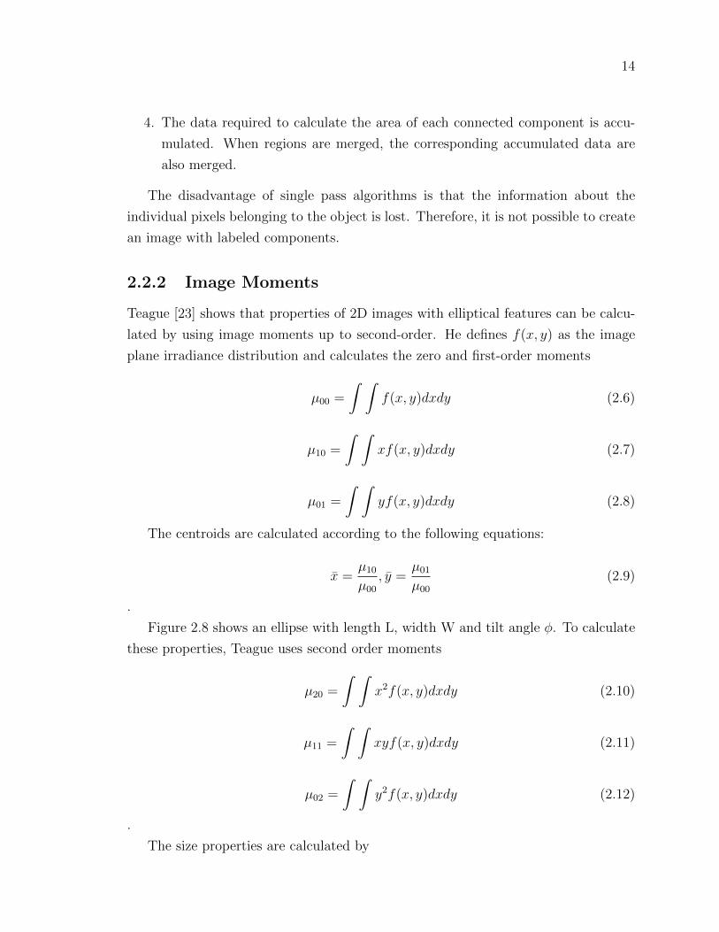
Figure 2.8 shows an ellipse with length L, width W and tilt angle φ. To calculate

these properties, Teague uses second order moments

µ20 =

∫ ∫x2f(x, y)dxdy (2.10)

µ11 =

∫ ∫xyf(x, y)dxdy (2.11)

µ02 =

∫ ∫y2f(x, y)dxdy (2.12)

.

The size properties are calculated by

15

Figure 2.8: Image ellipse with properties

L = 2.83

√µ20 + µ02 +

√(µ20 − µ02)

2 + 4µ211, (2.13)

W = 2.83

√µ20 + µ02 −

√(µ20 − µ02)

2 + 4µ211 (2.14)

for length and width, respectively and

φ =1

2tan−1

(2µ11

µ20 − µ02

)(2.15)

for tilt angle φ.

2.3 Chapter Summary

Ship detection algorithms in literature are all implemented with the assumption that

the image is present and accessible for the entirety of the algorithm. However, since

these are software algorithms, they tend to run slower than their hardware counter-

parts, making them hard to implement to be synchronous with the satellite. On the

other hand, even though there are theories on property calculation and even software

implementations, there is a lack of property calculation algorithms using hardware.

Thus, in the following chapter, a ship detection and property calculation algorithm

is proposed that can be implemented to be synchronous with the satellite.

16

Chapter 3

Proposed Algorithm for Detection

and Characterization of Ships in

SAR Images

3.1 Reason for considerations

Before extracting the properties of the ships, the proposed algorithm should first

detect the ships. According to the statistical tests concluded on distributions, the

exponential distribution was found as the best fit for single-look images while the

k-distribution was found as the best fit for multi-look images [24]. Therefore, since

this research uses single-look images for the hardware implementation of the ship

detection, an adaptive thresholding algorithm with exponential model is selected.

Single pass algorithms focus on extracting features during labeling instead of cre-

ating a labeled image. For Johnston et al. [22], as the feature of interest was the area

of a labeled region, they were accumulating the number of pixels that belong to the

region and using it as the area. By building upon the same idea, if the required values

are accumulated, it would be possible to extract more properties from the regions.

Since the calculations by [23] rely only on the moments, by accumulating the required

values for the moments for each ship, it is possible to extract the location, size and

orientation information from the SAR image using hardware. This approach would

allow for a streamlined approach which can be synchronized with the SAR system.

Since no ship detection algorithm is perfect, a discrimination step is also suggested

to reduce the false alarms. One way of discrimination is human supervision. Although

17

in [25] this approach is reported to be working well, there are also more automated

options. Liu et al. [26] use morphological operations to cluster neighboring pixels and

eliminate isolated detected pixels. Another approach is to cluster pixels that belong

to the same ship to compute some measurement such as area, length, width, etc. In

[27, 28], the size of the detected ship is used to discriminate detections. Since the

calculation of the properties is already a task of this thesis, discrimination using the

size of the detected ship is selected to be implemented.

3.2 Proposed Algorithm

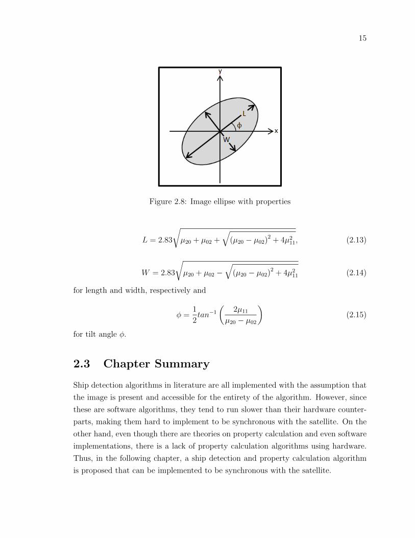
As also shown in Figure 3.1, the proposed algorithm consists of the following major

steps:

1. Thresholding

2. Clustering and Data Accumulation

3. Calculation of Ship Parameters

The thresholding step applies a ship detection algorithm to the input image to

identify ships. The clustering and data accumulation step checks connectivity of

detected pixels and if two or more pixels are connected, treats them as a single ship

as opposed to multiple ships. This step also extracts some intermediate data from

the detected pixels to be used in the property calculation step. Lastly, property

calculation step computes the location, size and orientation information for each

detected ship and does discrimination depending on the image size. The details of

each step are described in following sections.

Figure 3.1: Block diagram for the proposed algorithm

18

3.2.1 Thresholding

The thresholding part of the algorithm identifies pixels, which have values higher than

some predetermined threshold value and thus, identify ships. In the image formation

of SAR images on hardware, a frame of image is created once enough data is collected

and stored in a RAM while the data for the next frame is being collected. This creates

a time restraint for the hardware implementations whereas software applications do

not have this issue. Figure 3.2 shows how the frames are created. As it can be

observed while the satellite is moving, the antenna of the satellite scans the ground

using a single beam. Once enough data is recorded on the azimuth direction an image

frame is created. After the literature review, adaptive thresholding algorithm with

exponential model was selected for the hardware implementation as it is best suited

for single-look images. This algorithm checks the average power level of the pixels

around the pixel under test (PUT), and if PUT is higher than the average scaled by

a design parameter, that pixel is registered as detection. However, since ships are

usually more than a single pixel in a SAR image, the immediately adjacent pixels

are omitted while calculating the average to ensure the pixels used to calculate the

average only belong to the ocean. This calculation is done for every pixel of the image

to detect ships. As briefly explained in Section 2.1, this method implements three

nested windows called background, buffer and signal window. Signal window is the

pixel being tested; buffer window is the buffer zone and background window where

the average is calculated.

Figure 3.2: Frames of the SAR image

Figure 3.3(a) shows the traditional nested windows. Generally, the windows are

made of boxes. For example, 1x1 window for signal, 5x5 window for buffer and 7x7

19

for background window. The size of the buffer window is selected according to the

biggest expected ship in the image, to create an adequate buffer zone. Background

window, on the other hand is selected according to the model chosen to represent

the ocean, where more complex models require a higher number of samples, meaning

a bigger window. For each tested pixel, the number of pixels read to calculate the

average is the background window size subtracted by the buffer window size. In

the example case, this number is but can change depending on window sizes. This

means to threshold each pixel in the entire image, the memory needs to be accessed

25 times the number of pixels in the image. However, in this thesis, instead of a

2D window, a 1D window is proposed as illustrated in Figure 3.3(b). This stops the

need for accessing the image multiple times per each pixel, and thus the image can

be streamed with full speed, making the ship detection algorithm real time.

Figure 3.3: Nested windows: (a) 2D nested windows, (b) 1D nested windows

For each frame, the following steps are used for ship detection:

1. For each pixel calculate the mean of the background window µb.

2. Calculate threshold as Tµb.

3. Compare the current pixel value with the threshold.

4. Return detection flag if the tested pixel value is higher than the threshold.

In these steps, µb is the mean of the background window and T is the design

parameter. By using the guideline of choosing design parameters by [17] and testing

different values, the design parameter T was selected as 5. Figure 3.4 shows the input

and output of the thresholding step. Figure 3.4(a) shows a ship in an ocean, 3.4(b)

20

shows the binary output of detections in image format. The white pixels show the

detections as binary 1 while the black pixels show the pixels failed the thresholding

test as binary 0.

Figure 3.4: Thresholding: (a) Original image, (b) binary image after thresholding

3.2.2 Clustering and Data Accumulation

Depending on the resolution of the satellite and the ship size, a ship can be rep-

resented by more than a single pixel in the image. This creates a need for an al-

gorithm that can connect neighboring pixels to correctly represent each individual

ship by pixels belonging to it. On the other hand, calculating the parameters of

ships require some intermediate values to calculate image moments per ship such as∑x,∑x2,∑y,∑y2,∑xy and N. x and y are the range and azimuth coordinates of

an individual pixel that belongs to the ship while N is the number of pixels belonging

to the same ship. By integrating a data accumulation step that runs in parallel with

clustering, the need for an additional scan of the image was omitted. The clustering

and data accumulation step is divided into two sub-steps: labeling and merging. La-

beling connects vertically connected pixels while merging connects the labeled vertical

pixels, horizontally. The algorithm for labeling consists of the following steps and is

also pictorially described in Figure 3.5:

1. Look at each individual detection (C).

2. Look at the pixel above current pixel (U).

21

3. If U is not a detected pixel, increase the label number by 1 and label the current

pixel with the new label number.

4. If U is a detection, add pixel data, (x,x2,y,y2,xy), where x and y are row and

column of C to the current data stored at that label; increase number of pixels

at that label (N) by one.

5. The data stored at each label will be used to compute the size and orientation

of each ship in the latter section of the algorithm.

Figure 3.5: Flowchart for labeling

The end result of the labeling portion of the algorithm is all the pixels in the same

column are combined together under one label and their pixel data (x,x2,y,y2,xy) is

added together and stored. The result is shown in Figure 3.6 with different colors

identifying different labels. The labeling step completes when the entire image is

processed.

22

Figure 3.6: Labeling: (a) Binary image, (b) after labeling each color represents adifferent label

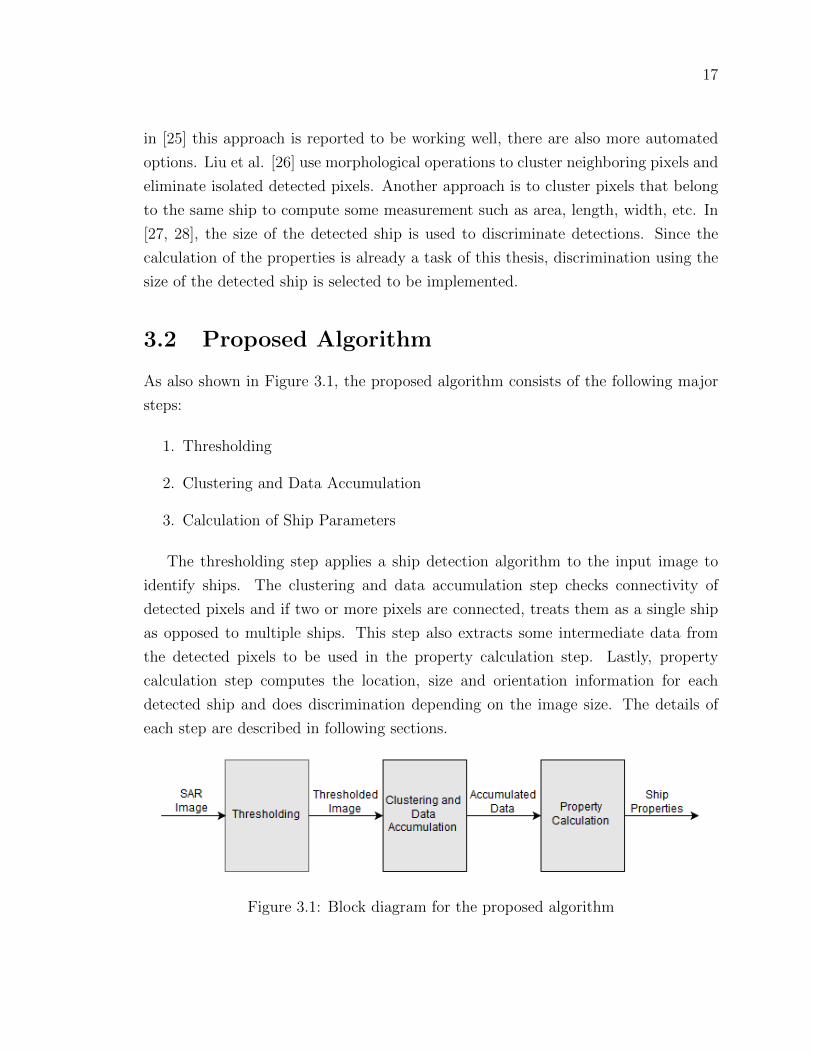
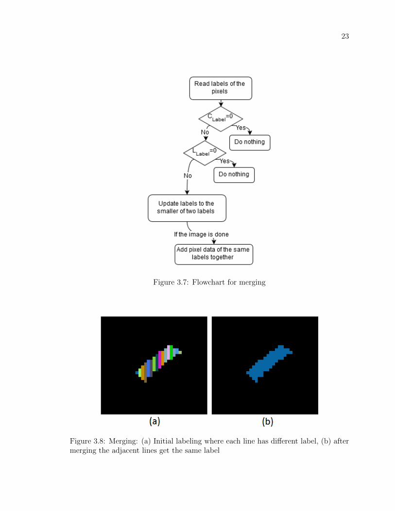
The next step is to merge all the individual identified columns into one label,

identifying one ship. The following are the steps of the merging algorithm and is also

pictorially described in Figure 3.7:

1. Initialize a merger table where each address refers to a label, i.e., value at

position 0 is 0, value at position 1 is 1 and so on.

2. For each pixel (C) look to the left (L) to find an adjacent column which will be

part of the same ship.

3. Lookup the label of the adjacent column.

4. Update label of the current column with the label of the adjacent column.

5. Add together pixel information (x,x2,y,y2,xy) of all pixels with the same label.

After the initialization on step 1, steps 2-4 are done in parallel with the labeling

step. The final step 5, is processed after the entire image is processed and only goes

over the label list. The result of the merging is shown in Figure 3.8. The labeled image

before merging is shown in 3.8(a) where only vertically connected pixels belong to

the same label. After merging, all connected pixels are labeled as the same as shown

in 3.8(b) where only two colors can be seen denoting two labels.

23

Figure 3.7: Flowchart for merging

Figure 3.8: Merging: (a) Initial labeling where each line has different label, (b) aftermerging the adjacent lines get the same label

24

3.2.3 Calculation of Ship Parameters

Using the pixel data (x,x2,y,y2,xy) and number of pixels N, per label stored previously

in clustering and the data accumulation step of the algorithm, ship properties are

computed using the equations from [23]. These equations were converted to discrete

form to be applied on the data.

The location of the ship is calculated by averaging the pixel locations of each pixel

belonging to the same cluster. As∑x is already accumulated and N is known. The

location is calculated as:

xc =

∑x

N(3.1)

yc =

∑y

N(3.2)

The calculation of the size and orientation of the ships uses more complex ap-

proach involving the image moments. First the second order moments, u20,u02,u11,

are calculated.

uxx =

∑x2

N− xc2 (3.3)

uyy =

∑y2

N− yc2 (3.4)

uxy = xcyc −∑xy

N(3.5)

During the calculation of the size and orientation, the following is a common

element and therefore, is calculated once to speed up the process.

C =√

(uxx − uyy)2 + 4uxy2 (3.6)

The length L, width W and orientation O is calculated using the following formula

L = 2.83√uxx + uyy + c (3.7)

W = 2.83√uxx + uyy − c (3.8)

O =

arctan

(uxx − uyy + C

2uxy

)if uyy > uxx

arctan

(2uxy

uxx − uyy + C

)else

(3.9)

25

After the calculations for each ship the following are acquired:

� Location (center) of the ship expressed in x,y coordinates;

� Length and width of the ship expressed in number of pixels;

� Orientation of the ship expressed in degrees in range (-90,90).

Before outputting, the ship size is compared to a minimum size parameter to

discriminate unwanted detections. For high resolution images, this value was selected

as 1 pixel to eliminate single pixel speckle noise. However, since in low resolution

images a ship can be a single pixel, this value was selected as 0.

The location of the ship is the most important information for maritime surveil-

lance which shows where the ship is, as well as if the ship is somewhere prohibited.

Size of the ship can be used to identify the ship type or even the ship itself as dif-

ferent ship types have different length-width ratios. On the other hand, orientation

of the ship can be used to determine the path of the ship. This information can

be cross checked by an automatic information system (AIS), to catch disinformation

from vessels.

3.3 Chapter Summary

In this chapter the proposed algorithm is introduced and explained. This algorithm

models the ocean using an exponential model and dynamically creates a threshold for

each pixel from the statistics of its surrounding. While connected pixels are labeled

to detect ships, data is accumulated. This data is then used to calculate properties

for each ship. In the next chapter, the software and hardware implementation of the

proposed algorithm is discussed.

26

Chapter 4

Implementation

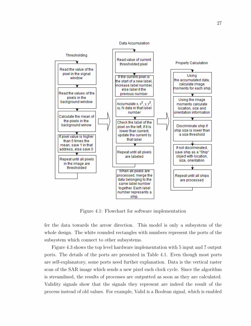
4.1 Software Implementation

The design was first implemented in Matlab to both validate the algorithm and to

set a reference. The code is provided in A.1 and a flowchart is provided in Figure

4.1. This code first goes over each pixel and uses the ship detection algorithm to

determine if the tested pixel is a detection. If so, according to the labeling algorithm,

its values are extracted and stored in that label location. Meanwhile, a merger table

is updated according to the neighboring pixel. After the image is processed, values

for neighboring labels are merged using the merger table. The values were used to

calculate the properties for each ship which is returned at the end of the process.

4.2 Hardware Implementation

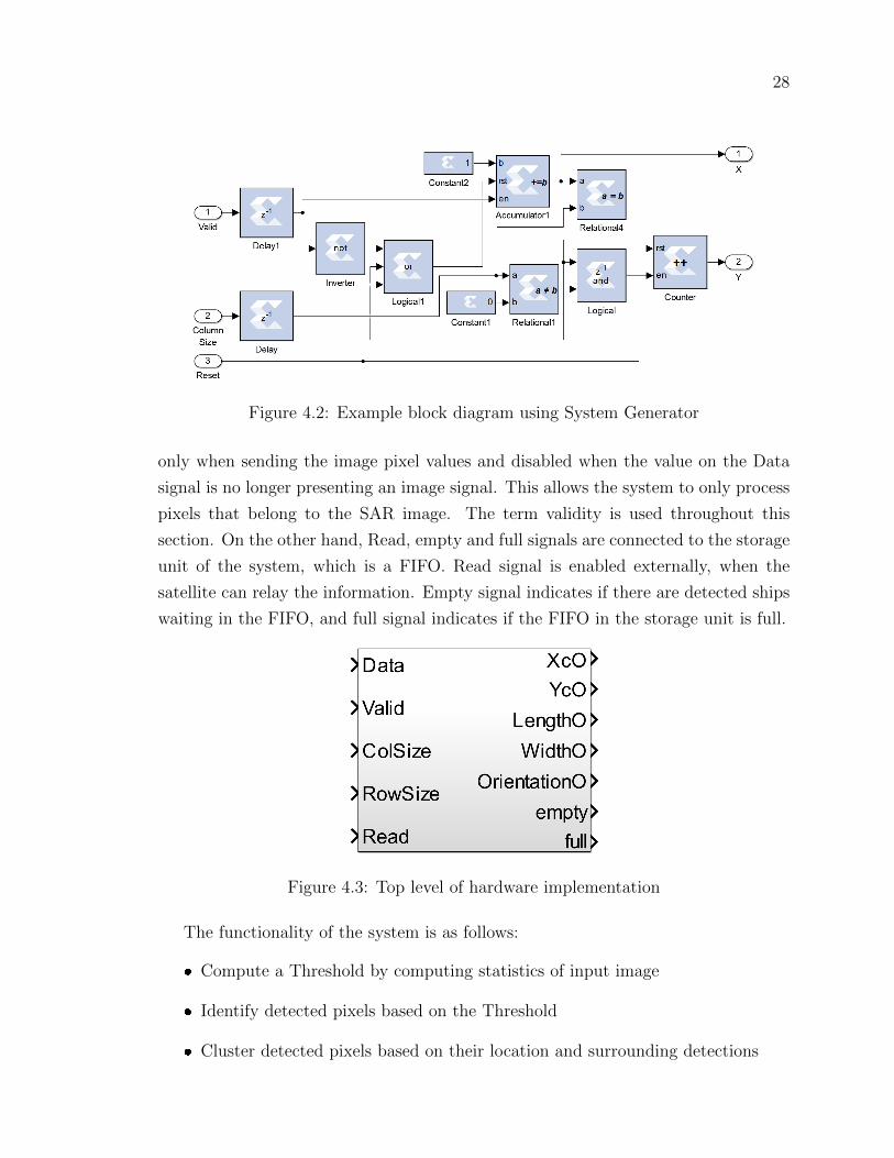
For the implementation of the design on hardware, Xilinx’s System Generator tool

[29] was used. System Generator is a tool that integrates with Matlab’s block di-

agramming tool Simulink, and provides its own library of blocks. The tool allows

for simulation through Matlab as well as co-simulation with communication between

software in Matlab and hardware on a FPGA. System Generator is also used to create

netlists from the block diagram to be used in Xilinx Integrated Synthesis Environment

(ISE). This approach was used for its ease of use and for its graphical representation.

It also shows the capabilities and potential of the tool. Figure 4.2 shows an example

block diagram model created by System Generator. In this model, the blue blocks

are provided by the tool’s library. These blocks are connected via lines which trans-

27

Figure 4.1: Flowchart for software implementation

fer the data towards the arrow direction. This model is only a subsystem of the

whole design. The white rounded rectangles with numbers represent the ports of the

subsystem which connect to other subsystems.

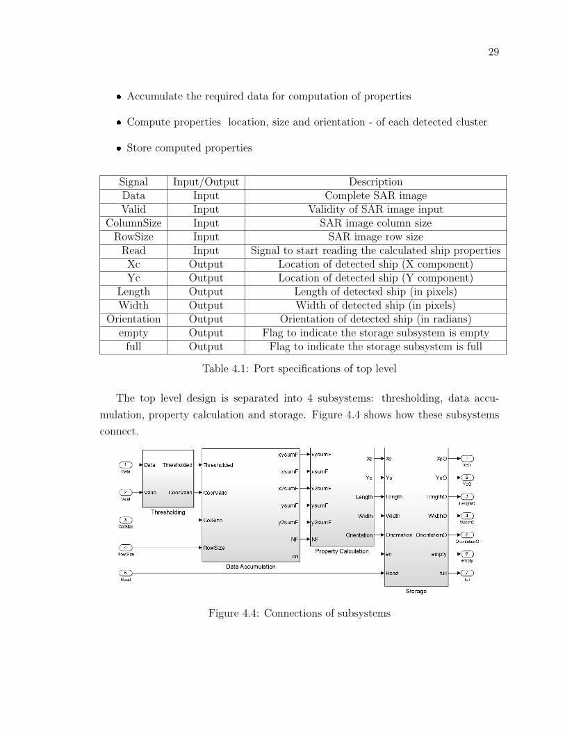
Figure 4.3 shows the top level hardware implementation with 5 input and 7 output

ports. The details of the ports are presented in Table 4.1. Even though most ports

are self-explanatory, some ports need further explanation. Data is the vertical raster

scan of the SAR image which sends a new pixel each clock cycle. Since the algorithm

is streamlined, the results of processes are outputted as soon as they are calculated.

Validity signals show that the signals they represent are indeed the result of the

process instead of old values. For example, Valid is a Boolean signal, which is enabled

28

Figure 4.2: Example block diagram using System Generator

only when sending the image pixel values and disabled when the value on the Data

signal is no longer presenting an image signal. This allows the system to only process

pixels that belong to the SAR image. The term validity is used throughout this

section. On the other hand, Read, empty and full signals are connected to the storage

unit of the system, which is a FIFO. Read signal is enabled externally, when the

satellite can relay the information. Empty signal indicates if there are detected ships

waiting in the FIFO, and full signal indicates if the FIFO in the storage unit is full.

Figure 4.3: Top level of hardware implementation

The functionality of the system is as follows:

� Compute a Threshold by computing statistics of input image

� Identify detected pixels based on the Threshold

� Cluster detected pixels based on their location and surrounding detections

29

� Accumulate the required data for computation of properties

� Compute properties location, size and orientation - of each detected cluster

� Store computed properties

Signal Input/Output DescriptionData Input Complete SAR imageValid Input Validity of SAR image input

ColumnSize Input SAR image column sizeRowSize Input SAR image row size

Read Input Signal to start reading the calculated ship propertiesXc Output Location of detected ship (X component)Yc Output Location of detected ship (Y component)

Length Output Length of detected ship (in pixels)Width Output Width of detected ship (in pixels)

Orientation Output Orientation of detected ship (in radians)empty Output Flag to indicate the storage subsystem is empty

full Output Flag to indicate the storage subsystem is full

Table 4.1: Port specifications of top level

The top level design is separated into 4 subsystems: thresholding, data accu-

mulation, property calculation and storage. Figure 4.4 shows how these subsystems

connect.

Figure 4.4: Connections of subsystems

30

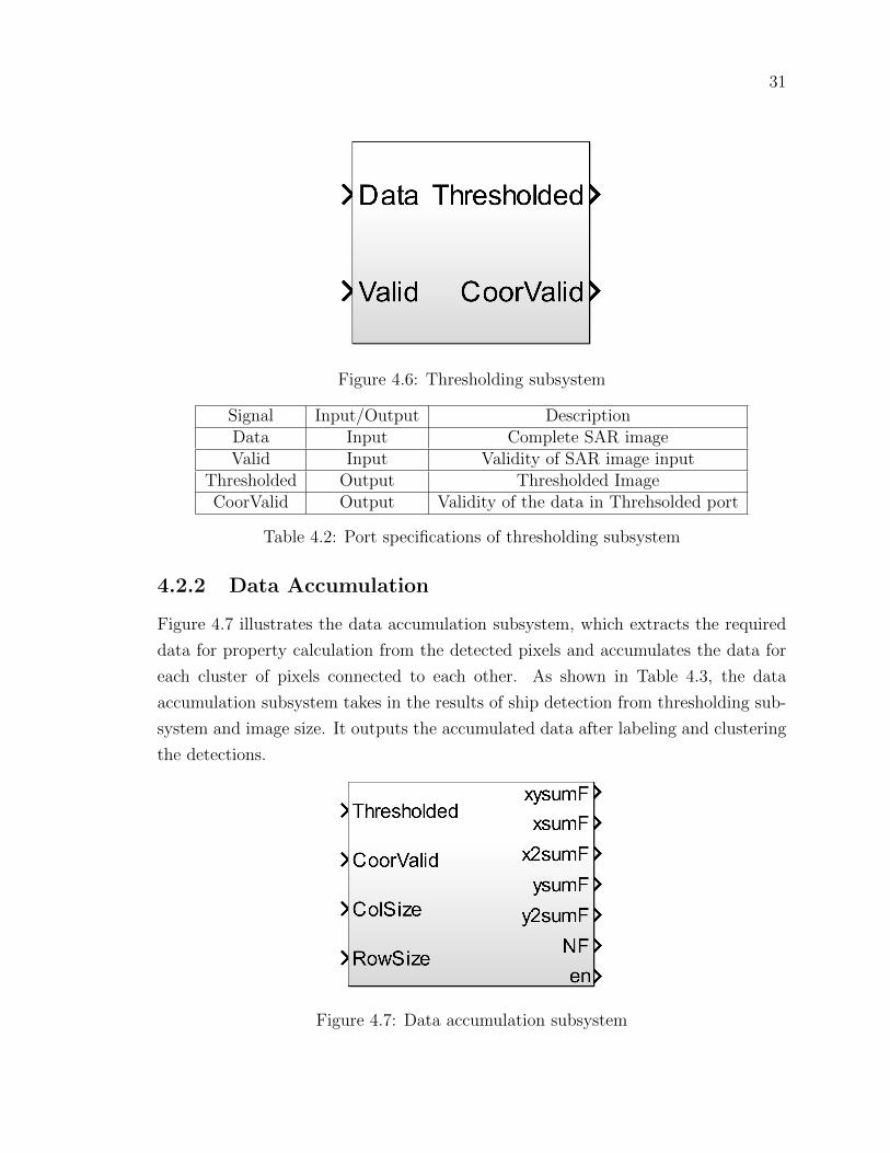
4.2.1 Thresholding

Figure 4.6 illustrates the thresholding subsystem, which uses the adaptive threshold

algorithm to apply a binary threshold to each pixel of the image. For the hardware

implementation of the ship detection algorithm, a variation of [30] was used. Figure

4.5 shows the structure of the thresholding algorithm. X is an array of image pixels

in the background window, Y is the tested pixel value, T is the design parameter for

the algorithm and e(Y) is the result of the algorithm. The value of the tested pixel is

compared to the average of stored background values scaled by the design parameter

and a Boolean signal is returned. As shown in Table 4.2, this subsystem takes in the

SAR image pixel value and the valid signal and outputs a Boolean signal of 1 or 0

depending on the detection with a valid signal of its own.

Figure 4.5: Structure of thresholding algorithm

The functionality of this subsystem is as follows:

1. Get the new pixel value (XN+1 when testing Y+1), adding it to the background

window and dropping the pixel that is at the end of the background window,

e.g., X1 when testing Y+1.

2. Compute threshold as the average of background pixels scaled by the design

parameter T. T is selected as 5 for reasons explained in Section 3.2.1.

3. Compare the pixel value in the target window to the threshold.

4. Output 1 if pixel value is higher than threshold, else output 0.

5. Return to step 1.

31

Figure 4.6: Thresholding subsystem

Signal Input/Output DescriptionData Input Complete SAR imageValid Input Validity of SAR image input

Thresholded Output Thresholded ImageCoorValid Output Validity of the data in Threhsolded port

Table 4.2: Port specifications of thresholding subsystem

4.2.2 Data Accumulation

Figure 4.7 illustrates the data accumulation subsystem, which extracts the required

data for property calculation from the detected pixels and accumulates the data for

each cluster of pixels connected to each other. As shown in Table 4.3, the data

accumulation subsystem takes in the results of ship detection from thresholding sub-

system and image size. It outputs the accumulated data after labeling and clustering

the detections.

Figure 4.7: Data accumulation subsystem

32

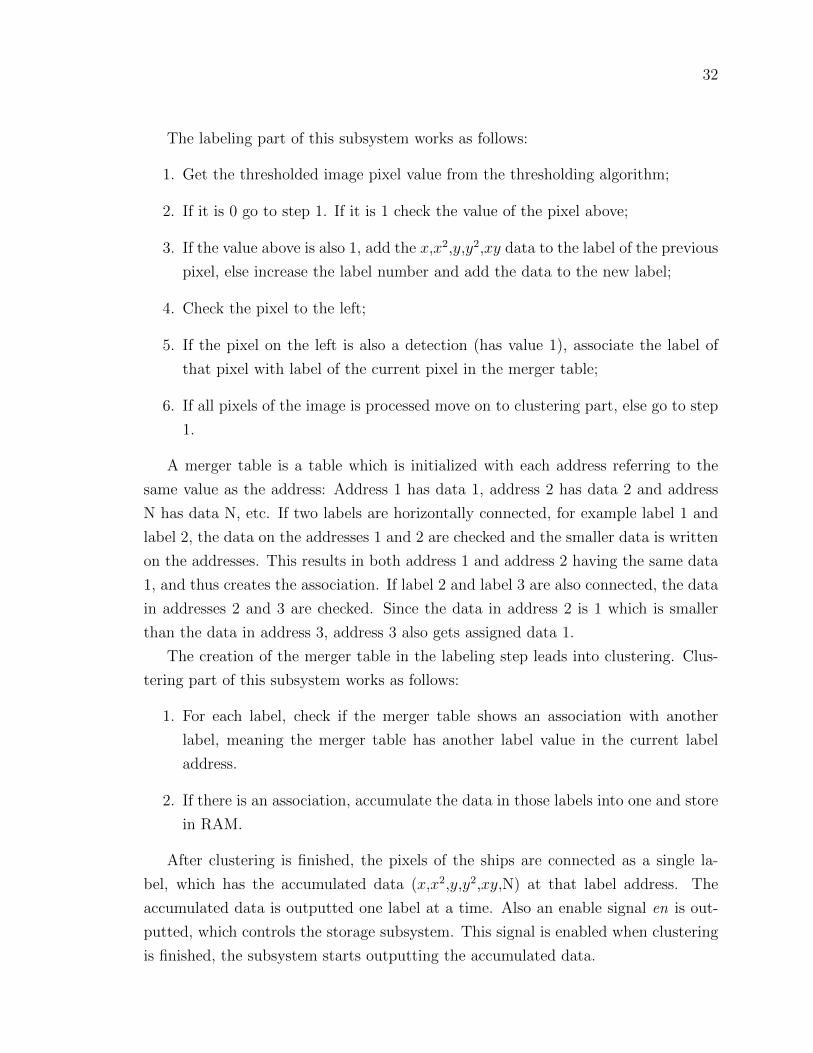
The labeling part of this subsystem works as follows:

1. Get the thresholded image pixel value from the thresholding algorithm;

2. If it is 0 go to step 1. If it is 1 check the value of the pixel above;

3. If the value above is also 1, add the x,x2,y,y2,xy data to the label of the previous

pixel, else increase the label number and add the data to the new label;

4. Check the pixel to the left;

5. If the pixel on the left is also a detection (has value 1), associate the label of

that pixel with label of the current pixel in the merger table;

6. If all pixels of the image is processed move on to clustering part, else go to step

1.

A merger table is a table which is initialized with each address referring to the

same value as the address: Address 1 has data 1, address 2 has data 2 and address

N has data N, etc. If two labels are horizontally connected, for example label 1 and

label 2, the data on the addresses 1 and 2 are checked and the smaller data is written

on the addresses. This results in both address 1 and address 2 having the same data

1, and thus creates the association. If label 2 and label 3 are also connected, the data

in addresses 2 and 3 are checked. Since the data in address 2 is 1 which is smaller

than the data in address 3, address 3 also gets assigned data 1.

The creation of the merger table in the labeling step leads into clustering. Clus-

tering part of this subsystem works as follows:

1. For each label, check if the merger table shows an association with another

label, meaning the merger table has another label value in the current label

address.

2. If there is an association, accumulate the data in those labels into one and store

in RAM.

After clustering is finished, the pixels of the ships are connected as a single la-

bel, which has the accumulated data (x,x2,y,y2,xy,N) at that label address. The

accumulated data is outputted one label at a time. Also an enable signal en is out-

putted, which controls the storage subsystem. This signal is enabled when clustering

is finished, the subsystem starts outputting the accumulated data.

33

Signal Input/Output DescriptionThresholded Input Thresholded ImageCoorValid Input Validity of the data in Threhsolded port

ColumnSize Input SAR image column sizeRowSize Input SAR image row sizexysumF Output

∑xy for each ship

xsumF Output∑x for each ship

x2sumF Output∑x2 for each ship

ysumF Output∑y for each ship

y2sumF Output Accumulated∑x for each ship

NF Output Number of pixels belonging to the same shipen Output Write enable for storage subsystem

Table 4.3: Port specifications of data accumulation subsystem

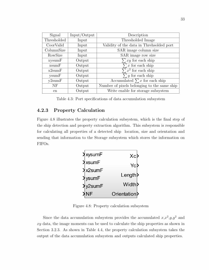
4.2.3 Property Calculation

Figure 4.8 illustrates the property calculation subsystem, which is the final step of

the ship detection and property extraction algorithm. This subsystem is responsible

for calculating all properties of a detected ship location, size and orientation and

sending that information to the Storage subsystem which stores the information on

FIFOs.

Figure 4.8: Property calculation subsystem

Since the data accumulation subsystem provides the accumulated x,x2,y,y2 and

xy data, the image moments can be used to calculate the ship properties as shown in

Section 3.2.3. As shown in Table 4.4, the property calculation subsystem takes the

output of the data accumulation subsystem and outputs calculated ship properties.

34

Signal Input/Output DescriptionxysumF Input

∑xy for each ship

xsumF Input∑x for each ship

x2sumF Input∑x2 for each ship

ysumF Input∑y for each ship

y2sumF Input Accumulated∑x for each ship

NF Input Number of pixels belonging to the same shipXc Output Location of detected ship (X component) to storeYc Output Location of detected ship (Y component) to store

Length Output Length of detected ship (in pixels) to storeWidth Output Width of detected ship (in pixels) to store

Orientation Output Orientation of detected ship (in radians) to store

Table 4.4: Port specifications of property calculation subsystem

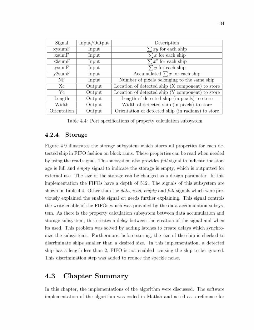
4.2.4 Storage

Figure 4.9 illustrates the storage subsystem which stores all properties for each de-

tected ship in FIFO fashion on block rams. These properties can be read when needed

by using the read signal. This subsystem also provides full signal to indicate the stor-

age is full and empty signal to indicate the storage is empty, which is outputted for

external use. The size of the storage can be changed as a design parameter. In this

implementation the FIFOs have a depth of 512. The signals of this subsystem are

shown in Table 4.4. Other than the data, read, empty and full signals which were pre-

viously explained the enable signal en needs further explaining. This signal controls

the write enable of the FIFOs which was provided by the data accumulation subsys-

tem. As there is the property calculation subsystem between data accumulation and

storage subsystem, this creates a delay between the creation of the signal and when

its used. This problem was solved by adding latches to create delays which synchro-

nize the subsystems. Furthermore, before storing, the size of the ship is checked to

discriminate ships smaller than a desired size. In this implementation, a detected

ship has a length less than 2, FIFO is not enabled, causing the ship to be ignored.

This discrimination step was added to reduce the speckle noise.

4.3 Chapter Summary

In this chapter, the implementations of the algorithm were discussed. The software

implementation of the algorithm was coded in Matlab and acted as a reference for

35

Figure 4.9: Storage subsystem

Signal Input/Output DescriptionXc Input Location of detected ship (X component) to storeYc Input Location of detected ship (Y component) to store

Length Input Length of detected ship (in pixels) to storeWidth Input Width of detected ship (in pixels) to store

Orientation Input Orientation of detected ship (in radians) to storeen Input Write enable for storage subsystem

Read Input Signal to start reading the calculated ship propertiesXcO Output Location of stored ship (X component)YcO Output Location of stored ship (Y component)

LengthO Output Length of stored ship (in pixels)WidthO Output Width of stored ship (in pixels)

OrientationO Output Orientation of stored ship (in radians)empty Output Flag to indicate the storage is empty

full Output Flag to indicate the storage is full

Table 4.5: Port specifications of storage subsystem

the hardware implementation. The hardware implementation on the other hand, was

designed and simulated using System Generator with the addition of the storage sub-

system. The hardware block diagram was then converted into a hardware description

language and programmed in to a xc7k325t board for final test. For both imple-

mentations, single-look RADARSAT-2 test images were used. The following chapter

shows the results and evaluation of the algorithm.

36

Chapter 5

Experimental Work

5.1 Setup

To test the proposed algorithm three experiments were conducted:

1. Ship Detection on a standard resolution SAR image using software.

2. Ship Detection on a standard resolution SAR image using hardware.

3. Ship Detection on a high resolution SAR image using hardware.

5.1.1 Experiment 1: Ship Detection on a low resolution SAR

image using software

The objective of this experiment is to evaluate the accuracy of the ship detection step

of the proposed algorithm. For this purpose, 36 horizontally polarized single-look

RADARSAT-2 test images were used. However, since these images were proprietary

materials of Macdonald Dettwiler and Associates (MDA), only the results of the

algorithm will be shown. These images have 40 meter resolution and their size is

roughly 15000x20000 pixels. These test images were used with the software design in

Matlab using a computer with an Intel I7 processor, 8GB ram and 64 bit operating

system. In this experiment, background window was selected as 21 and the buffer

window was selected as 11. The threshold design parameter was selected as 5. Since

these were low resolution images, the minimum size parameters were selected as 1 to

reduce single pixel speckle noise.

37

5.1.2 Experiment 2: Ship Detection on a low resolution SAR

image using hardware

The objective of this experiment is to evaluate the hardware implementation of the

ship detection algorithm. The images from the first experiment were used to compare

the accuracy to the software implementation. Each image was flattened into a 1-

D array column after column. The array was then turned into timeseries format.

Timeseries format consists of two arrays. One is the data array and the other is the

time array. The nth element of the data array is sent to the port at time referred

by nth element of the data array. In this case, each element of the data array was

assigned to another clock cycle. Then another timeseries, valid, was created, where

the elements of the data array are 1 at the same clock cycles as when the image data

is present, and 0 on other clock cycles. The information about the size of the image

was also provided in RowSize and ColumnSize ports. A constant 1 was given to the

Read port so the parameters were outputted as soon as they are available.

5.1.3 Experiment 3: Ship Detection on a high resolution

SAR image using hardware

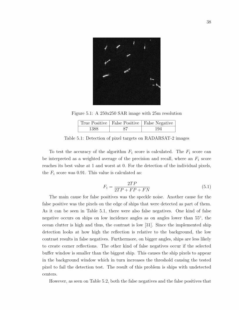
In this experiment, a 250x250 SAR image, shown in Figure 5.1, is used. This image

has 25m resolution and contains 12 ships. The objective of this experiment was to

see if the algorithm can correctly detect the ships and calculate the properties of

the ships. Since the resolution is higher in this experiment, the minimum ship size

parameters were increased to 2 to further reduce the speckle noise.

5.2 Analysis

5.2.1 Experiment 1 Analysis

Before moving on to the detection of ships, the detection of the individual pixels that

passed the thresholding was analyzed. The test data consists of targets we assume

to create certain number of pixels passing the test depending on their shape. This

is used as the ground truth to check the accuracy of the thresholding algorithm.

Table 5.1 shows the total true positive, false positive and false negative results of the

experiment.

38

Figure 5.1: A 250x250 SAR image with 25m resolution

True Positive False Positive False Negative1388 87 194

Table 5.1: Detection of pixel targets on RADARSAT-2 images

To test the accuracy of the algorithm F1 score is calculated. The F1 score can

be interpreted as a weighted average of the precision and recall, where an F1 score

reaches its best value at 1 and worst at 0. For the detection of the individual pixels,

the F1 score was 0.91. This value is calculated as:

F1 =2TP

2TP + FP + FN(5.1)

The main cause for false positives was the speckle noise. Another cause for the

false positive was the pixels on the edge of ships that were detected as part of them.

As it can be seen in Table 5.1, there were also false negatives. One kind of false

negative occurs on ships on low incidence angles as on angles lower than 55◦, the

ocean clutter is high and thus, the contrast is low [31]. Since the implemented ship

detection looks at how high the reflection is relative to the background, the low

contrast results in false negatives. Furthermore, on bigger angles, ships are less likely

to create corner reflections. The other kind of false negatives occur if the selected

buffer window is smaller than the biggest ship. This causes the ship pixels to appear

in the background window which in turn increases the threshold causing the tested

pixel to fail the detection test. The result of this problem is ships with undetected

centers.

However, as seen on Table 5.2, both the false negatives and the false positives that

39

are connected to ships had little to no effect on the detection on total number of ships.

This is due to the ground truth was based on the target shape. However, the only

thing that had a major effect on the final outcome was the false positives. Even though

most of the speckle noise was removed by discriminating single pixel detections, false

detections consisting of 2 or more connected pixels passed the discrimination. These

detections were interpreted as targets thus lowering the accuracy of the ship detection.

Therefore we think discrimination step is more important in this context. For the

detection of targets, the F1 score was 0.98.

True Positive False Positive False Negative324 13 0

Table 5.2: Detection of targets on RADARSAT-2 images on software

The software implementation takes 37 seconds on average to process images.

5.2.2 Experiment 2 Analysis

Table 5.3 shows the resource utilization of the hardware implementation. In this

table flip-flop, look-up-table, dsp48 slices (a math oriented hardware component) and

block ram resources usage are given. The dsp48 was used in math intensive blocks

such as square root and to reduce the use of look-up-tables which could take up

considerable space on hardware. BRAM on the other hand was used as memory

to store both intermediate label values and as FIFOs. Since the calculation of the

properties is computationally intensive and is done in streamline fashion, the relatively

high utilization was expected. This is due to the tradeoff between performance and

utilization where in this case performance was chosen to be the main focus.

Used Available PercentageFF 10304 407600 2.5%

LUT 8247 203800 4%DSP48 48 840 5.7%BRAM 30 445 6.7%

Table 5.3: Utilization of the algorithm on hardware

The total on chip power was 0.402 W when working on a 65 MHz clock frequency,

which is the master clock frequency of RADARSAT-2 [3]. The hardware system took

an average of 6 seconds to process each image.

40

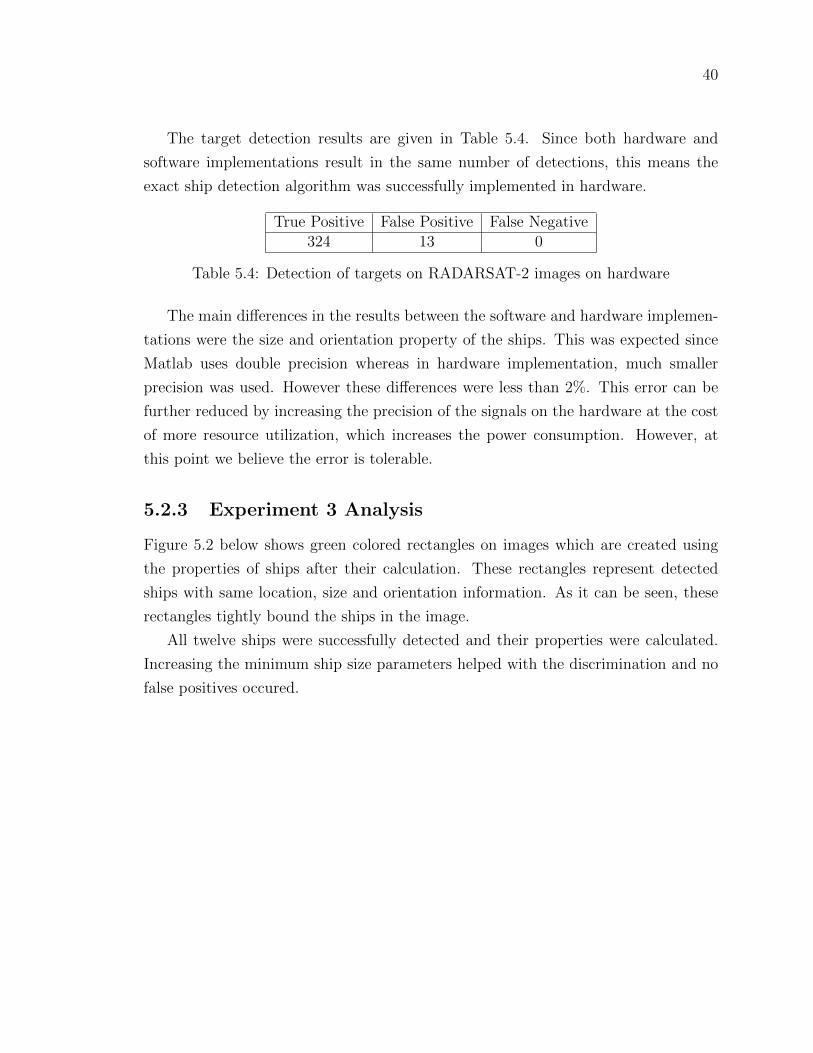
The target detection results are given in Table 5.4. Since both hardware and

software implementations result in the same number of detections, this means the

exact ship detection algorithm was successfully implemented in hardware.

True Positive False Positive False Negative324 13 0

Table 5.4: Detection of targets on RADARSAT-2 images on hardware

The main differences in the results between the software and hardware implemen-

tations were the size and orientation property of the ships. This was expected since

Matlab uses double precision whereas in hardware implementation, much smaller

precision was used. However these differences were less than 2%. This error can be

further reduced by increasing the precision of the signals on the hardware at the cost

of more resource utilization, which increases the power consumption. However, at

this point we believe the error is tolerable.

5.2.3 Experiment 3 Analysis

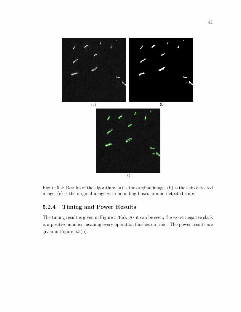
Figure 5.2 below shows green colored rectangles on images which are created using

the properties of ships after their calculation. These rectangles represent detected

ships with same location, size and orientation information. As it can be seen, these

rectangles tightly bound the ships in the image.

All twelve ships were successfully detected and their properties were calculated.

Increasing the minimum ship size parameters helped with the discrimination and no

false positives occured.

41

Figure 5.2: Results of the algorithm: (a) is the original image, (b) is the ship detectedimage, (c) is the original image with bounding boxes around detected ships

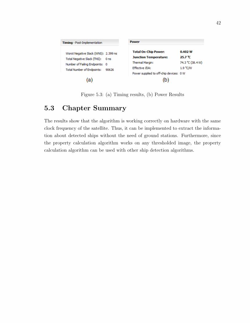
5.2.4 Timing and Power Results

The timing result is given in Figure 5.3(a). As it can be seen, the worst negative slack

is a positive number meaning every operation finishes on time. The power results are

given in Figure 5.3(b).

42

Figure 5.3: (a) Timing results, (b) Power Results

5.3 Chapter Summary

The results show that the algorithm is working correctly on hardware with the same

clock frequency of the satellite. Thus, it can be implemented to extract the informa-

tion about detected ships without the need of ground stations. Furthermore, since

the property calculation algorithm works on any thresholded image, the property

calculation algorithm can be used with other ship detection algorithms.

43

Chapter 6

Conclusion, Contributions and

Future Work

6.1 Conclusion

Ship detection on SAR images is done using the fact that ships return more of the

radar waves due to corner reflection, making them appear brighter. An adaptive

threshold uses the information of the pixels surrounding the tested pixels to create a

threshold which is then compared to the value of the pixel to determine if the pixel

is detection. Even though there are methods that use the waves of the ships this

method requires a specific type of polarization and is not reliable. Since the data

is streamlined, it was decided to accumulate all the data required to compute the

properties of the ships. After the data is accumulated, image moments are used to

calculate the properties.

The hardware implementation was able to detect the same pixels as the software

implementation with small differences in the properties. The proposed algorithm can

take the data in a stream and produce immediate information without the need of a

ground station allowing a quicker response to the results if needed. Furthermore, since

the property calculation algorithm works on any thresholded image, this algorithm

can be used with other ship detection algorithms.

44

6.2 Contributions

In this thesis, the following contributions were made to the problem of dependency

of satellites to ground stations to transfer the image data:

� A hardware solution to this problem was suggested to reduce the size of data

to only the information needed about ships on the image.

� An existing ship detection method was implemented on hardware and an al-

gorithm that can calculate the location, size and orientation properties of the

detected ships was developed.

� This algorithm combined with ship detection was implemented on hardware

and evaluated.

6.3 Future Work

This work provided a hardware ship detection and property extraction algoritm for

single-look radar images. The work can be extended further in the following direc-

tions:

1. Detecting movement of ships

2. Multi-look images

3. Land masking

6.3.1 Detecting movement of ships

Although the proposed algorithm can extract the location, size and orientation prop-

erties of ships, it cannot detect the speed. More work in the area is required to extract

further properties of ships. More information can be used to better classify the ships

and assess the danger.

6.3.2 Multi-look images

Unlike single-look images, which are created by the coverage in mind, multi-look

images are created by focusing on the same area during the imaging session. Multiple

45

images are taken from different antenna locations and averaged to reduced speckle

noise [32]. However, this changes the model of the ocean.

For multi-look SAR images, k-distribution was found as the best fit to model

the ocean behavior [24]. By using multi-look images and k-distribution model, false

detections can be reduced.

6.3.3 Land Masking

If the targeted area to be imaged includes land, ship detection algorithms can make

false detections because of the return from the land. Thus, the next step to improve

the algorithm is to add an initial step of land masking.

Robertson et al. [33] use pre-existing geographic maps to mask the land by regis-

tering the satellite orbit parameters to layover the map on the image. However, it is

noted that registration errors up to 2 kilometers can occur. To overcome this problem

they use a buffer zone of 2 kilometers along the coastline. To avoid the problem of

registration errors, Ferrara et al. [34] suggest a 5 step method for automatic detection

of coastlines:

1. Filter to remove speckle.

2. Apply an edge operator.

3. Dilate edge map with a mean filter.

4. Threshold the edge map histogram.

5. Apply a contour following algorithm.

A minimum land area constraint is also used to avoid using ships as masks. In the

future, a land masking algorithm can be added as the preprocessing step, allowing

the algorithm to work on close to shores and islands.

46

References

[1] G. W. Stimson, Introduction to airborne radar. SciTech Pub., 1998.

[2] C. R. Jackson, J. R. Apel, et al., Synthetic aperture radar marine user’s manual.

US Department of Commerce, National Oceanic and Atmospheric Administra-

tion, National Environmental Satellite, Data, and Information Serve, Office of

Research and Applications, 2004.

[3] MDA, “Radarsat-2 product description,” RN-SP-52-1238, no. 1/11, 2014.

[4] C. Oliver and S. Quegan, Understanding synthetic aperture radar images. SciTech

Publishing, 2004.

[5] M. Rey, J. Tunaley, J. Folinsbee, P. Jahans, J. Dixon, and M. Vant, “Applica-

tion of radon transform techniques to wake detection in seasat-a sar images,”

Geoscience and Remote Sensing, IEEE Transactions on, vol. 28, pp. 553–560,

Jul 1990.

[6] A. Copeland, G. Ravichandran, and M. Trivedi, “Localized radon transform-

based detection of ship wakes in sar images,” Geoscience and Remote Sensing,

IEEE Transactions on, vol. 33, pp. 35–45, Jan 1995.

[7] A. M. Reed and J. H. Milgram, “Ship wakes and their radar images,” Annual

Review of Fluid Mechanics, vol. 34, no. 1, pp. 469–502, 2002.

[8] I. Hennings, R. Romeiser, W. Alpers, and A. Viola, “Radar imaging of kelvin

arms of ship wakes,” International Journal of Remote Sensing, vol. 20, no. 13,

pp. 2519–2543, 1999.

[9] D. J. Crisp, “The state-of-the-art in ship detection in synthetic aperture radar

imagery,” tech. rep., DTIC Document, 2004.

47

[10] K. Eldhuset, “An automatic ship and ship wake detection system for spaceborne

sar images in coastal regions,” Geoscience and Remote Sensing, IEEE Transac-

tions on, vol. 34, pp. 1010–1019, Jul 1996.

[11] P. Vachon, J. Campbell, C. Bjerkelund, F. Dobson, and M. Rey, “Ship detec-

tion by the radarsat sar: Validation of detection model predictions,” Canadian

Journal of Remote Sensing, vol. 23, no. 1, pp. 48–59, 1997.

[12] I.-I. Lin, L. K. Kwoh, Y.-C. Lin, and V. Khoo, “Ship and ship wake detec-

tion in the ers sar imagery using computer-based algorithm,” in Geoscience and

Remote Sensing, 1997. IGARSS ’97. Remote Sensing - A Scientific Vision for

Sustainable Development., 1997 IEEE International, vol. 1, pp. 151–153 vol.1,

Aug 1997.

[13] J. Serra and P. Soille, Mathematical morphology and its applications to image

processing, vol. 2. Springer Science & Business Media, 2012.

[14] C. C. Wackerman, K. S. Friedman, W. G. Pichel, P. Clemente-Colon, and X. Li,

“Automatic detection of ships in radarsat-1 sar imagery,” Canadian Journal of

Remote Sensing, vol. 27, no. 5, pp. 568–577, 2001.

[15] S. Kalson, “Adaptive array cfar detection,” Aerospace and Electronic Systems,

IEEE Transactions on, vol. 31, pp. 534–542, April 1995.

[16] H. Johnsen, “Multi-look versus single-look processing of synthetic aperture radar

images with respect to ocean wave spectra estimation,” International Journal of

Remote Sensing, vol. 13, no. 9, pp. 1627–1643, 1992.

[17] K. Friedman, C. Wackerman, F. Funk, K. Rowell, W. Pichel, P. Clemente-Colon,

and X. Li, “Validation of an automatic vessel detection algorithm using sar

data and known vessel fleet distributions,” in Geoscience and Remote Sensing

Symposium, 2000. Proceedings. IGARSS 2000. IEEE 2000 International, vol. 5,

pp. 2071–2073 vol.5, 2000.

[18] C. Wang, M. Liao, and X. Li, “Ship detection in sar image based on the alpha-

stable distribution,” Sensors, vol. 8, no. 8, pp. 4948–4960, 2008.

[19] J. Lee, D. Schuler, R. Lang, and K. Ranson, “K-distribution for multi-look pro-

cessed polarimetric sar imagery,” in Geoscience and Remote Sensing Symposium,

48

1994. IGARSS ’94. Surface and Atmospheric Remote Sensing: Technologies,

Data Analysis and Interpretation., International, vol. 4, pp. 2179–2181 vol.4,

Aug 1994.

[20] G. V. Weinberg, Coherent multilook radar detection for targets in KK-distributed

clutter. INTECH Open Access Publisher, 2012.

[21] D. R. Lee, S. H. Jin, P. C. Thien, and J. W. Jeon, “Fpga based connected

component labeling,” in Control, Automation and Systems, 2007. ICCAS ’07.

International Conference on, pp. 2313–2317, Oct 2007.

[22] C. Johnston and D. Bailey, “Fpga implementation of a single pass connected com-

ponents algorithm,” in Electronic Design, Test and Applications, 2008. DELTA

2008. 4th IEEE International Symposium on, pp. 228–231, Jan 2008.

[23] M. R. Teague, “Image analysis via the general theory of moments,” JOSA,

vol. 70, no. 8, pp. 920–930, 1980.

[24] Q. Jiang, S. Wang, D. Ziou, and A. Zaart, “Automatic detection for ship targets

in radarsat sar images from coastal regions,” in Vision interface, vol. 99, pp. 131–

137, 1999.

[25] M. D. Henschel, M. T. Rey, J. Campbell, and D. Petrovic, “Comparison of

probability statistics for automated ship detection in sar imagery,” in 1998 In-

ternational Conference on Applications of Photonic Technology, pp. 986–991,

International Society for Optics and Photonics, 1998.

[26] Y. Liu, M. Fang, Q. Feng, and L. Wang, “An automatic ship detection system

using ers sar images,” in Geoscience and Remote Sensing Symposium, 2003.

IGARSS’03. Proceedings. 2003 IEEE International, vol. 4, pp. 2656–2658, IEEE,

2003.

[27] N. Kourti, J. Shepherd, and J. Verbrgh, “Fishing boat detection by using sar

imagery,” in Ship Detection In Coastal Water Workshop Agenda, Canada, 2000.

[28] D. P. Casasent, W. Su, D. Turaga, N. Narusawa, and S. Ashizawa, “Sar ship

detection using new conditional contrast box filter,” in AeroSense’99, pp. 274–

284, International Society for Optics and Photonics, 1999.

[29] Xilinx, System Generator for DSP Reference Guide, July 2010.

49

[30] R. Cumplido, C. Torres, and S. Lopez, “On the implementation of an efficient

fpga-based cfar processor for target detection,” in Electrical and Electronics En-

gineering, 2004.(ICEEE). 1st International Conference on, pp. 214–218, IEEE,

2004.

[31] R. Touzi, “On the use of polarimetric sar data for ship detection,” in Geoscience

and Remote Sensing Symposium, 1999. IGARSS’99 Proceedings. IEEE 1999 In-

ternational, vol. 2, pp. 812–814, IEEE, 1999.

[32] P. Mather and B. Tso, Classification methods for remotely sensed data. CRC

press, 2009.

[33] N. Robertson, P. Bird, and C. Brownsword, “Ship surveillance using radarsat

scansar images,” in Ship Detection in Coastal Water Workshop Agenda, Canada,

2000.

[34] M. Ferrara and A. Torre, “Automatic moving targets detection using a rule-based

system: comparison between different study cases,” in Geoscience and Remote

Sensing Symposium Proceedings, 1998. IGARSS ’98. 1998 IEEE International,

vol. 3, pp. 1593–1595 vol.3, Jul 1998.

50

Appendix A

Appendix

A.1 Matlab Code for Software Implementation

function ShipDetection(sar image)

Ship=[];

% %%%%%%%%%%%%%%%%%%%%%%%%%%%%%%%%%%%%%%%%%%%%%%%%%%%%%%%%%%%%%%%%%%%%%%%%

% Thresholding

% %%%%%%%%%%%%%%%%%%%%%%%%%%%%%%%%%%%%%%%%%%%%%%%%%%%%%%%%%%%%%%%%%%%%%%%%

% Finding the sizes of the inputted Image

Xlength=size(sar image,1);

Ylength=size(sar image,2);

% Size of the Window

Back win=21

Buff win=11;

% Size threshold for discrimination

minLength=0;

minWidth=0;

% Turn image into 1-D array

Imm=sar image(:);

% Thresholding

Thresholded=zeros(1,length(Imm));

51

for i =1:length(Imm)

if ((i-(Back win-1)/2 ) > 1)

Ls=sum(Imm(i-(Back win-1)/2: i-(Buff win-1)/2));

else if ((i-(Buff-1)/2 ) > 1)

Ls=sum(Imm(1: i-(Buff win-1)/2));

else

Ls=0;

end

if ((i+(Back win-1)/2 ) < length(Imm))

Hs=sum(Imm(i(Buff win-1)/2: i+(Back win-1)/2));

else if ((i+(Buff win-1)/2 ) < length(Imm))

Hs=sum(Imm(i+(Buff win-1)/2):length(Imm));

else

Hs=0;

end

Threshold= (Ls+Hs)/(Back win-Buff Win);

Thresholded(i)=Imm(i)>Threshold;

end

% %%%%%%%%%%%%%%%%%%%%%%%%%%%%%%%%%%%%%%%%%%%%%%%%%%%%%%%%%%%%%%%%%%%%%%%%

% Labeling

% %%%%%%%%%%%%%%%%%%%%%%%%%%%%%%%%%%%%%%%%%%%%%%%%%%%%%%%%%%%%%%%%%%%%%%%%

% Variable Initialization

Imm=sar image(:);

Label=0; % Label #

RamSize=100000; % Number of Maximum Label Locations

RAM=linspace(1,RamSize,RamSize);

Labeled=zeros(1,Xlength*Ylength);

xsum=zeros(1,RamSize); % Sum of X

x2sum=zeros(1,RamSize); % Sum of Xˆ2

ysum=zeros(1,RamSize); % Sum of Y

y2sum=zeros(1,RamSize); % Sum of Yˆ2

xysum=zeros(1,RamSize); % Sum of X*Y

52

N=zeros(1,RamSize); % Number of Pixels

Finalxsum=zeros(1,RamSize); % Final Sum of X

Finalx2sum=zeros(1,RamSize); % Final Sum of Xˆ2

Finalysum=zeros(1,RamSize); % Final Sum of Y

Finaly2sum=zeros(1,RamSize); % Final Sum of Yˆ2

Finalxysum=zeros(1,RamSize); % Final Sum of X*Y

FinalN=zeros(1,RamSize); % Final Number of Pixels

% Labeling and Calculation of Sums

xx=0;

yy=1;

for i=1:length(Imm)

xx=xx+1;

if xx==Xlength+1

yy=yy+1;

xx=1;

end

if(i-1>0)

Cur=Thresholded(i);

Prev=Thresholded(i-1);

else

Cur=Thresholded(i);

Prev=0;

end

if(Cur==1)

% If the current pixel is the start of a new label, increase label number

if(Prev==0 | |xx==1)Label=Label+1;

end

Labeled(i)=Label;

xsum(Label)=xsum(Label)+xx; % Updating of Sum of X

x2sum(Label)=x2sum(Label)+xxˆ2; % Updating of Sum of Xˆ2

ysum(Label)=ysum(Label)+yy; % Updating of Sum of Y

y2sum(Label)=y2sum(Label)+yyˆ2; % Updating of Sum of Yˆ2

xysum(Label)=xysum(Label)+xx*yy; % Updating of Sum of X*Y

N(Label)=N(Label)+1; % Updating of Number of Pixels

53

% Connect the Current Pixel with the one on the left if applicable

if(i-Xlength>0 && Label>0 && Labeled(i-Xlength)>0)

if RAM(Label)<RAM(Labeled(i-Xlength))

RAM(Labeled(i-Xlength))=RAM(Label);

else

RAM(Label)=RAM(Labeled(i-Xlength));

end

end

else

Labeled(i)=0;

end

end

% %%%%%%%%%%%%%%%%%%%%%%%%%%%%%%%%%%%%%%%%%%%%%%%%%%%%%%%%%%%%%%%%%%%%%%%%

% Clustering

% %%%%%%%%%%%%%%%%%%%%%%%%%%%%%%%%%%%%%%%%%%%%%%%%%%%%%%%%%%%%%%%%%%%%%%%%

% Merging and Calculation of Final Sums

for i=1:RamSize

%Updating of Final Sum of X

Finalxsum(RAM(i))=Finalxsum(RAM(i))+xsum(i);

%Updating of Final Sum of Xˆ2

Finalx2sum(RAM(i))=Finalx2sum(RAM(i))+x2sum(i);

%Updating of Final Sum of Y

Finalysum(RAM(i))=Finalysum(RAM(i))+ysum(i);

%Updating of Final Sum of Yˆ2

Finaly2sum(RAM(i))=Finaly2sum(RAM(i))+y2sum(i);

%Updating of Final Sum of X*Y

Finalxysum(RAM(i))=Finalxysum(RAM(i))+xysum(i);

%Updating of Final Number of Pixels

FinalN(RAM(i))=FinalN(RAM(i))+N(i);

end

% %%%%%%%%%%%%%%%%%%%%%%%%%%%%%%%%%%%%%%%%%%%%%%%%%%%%%%%%%%%%%%%%%%%%%%%%

% Calculation of location, size and orientation for Ship Reports

% %%%%%%%%%%%%%%%%%%%%%%%%%%%%%%%%%%%%%%%%%%%%%%%%%%%%%%%%%%%%%%%%%%%%%%%%

% Calculation of Ship Locations

Xc=Finalxsum./FinalN;

Yc=Finalysum./FinalN;

54

% Calculation of Length, Width and Orientation

Orientation=zeros(1,length(Xc));

Length=zeros(1,length(Xc));

Width=zeros(1,length(Xc));

for i=1:RamSize

% Calculation of Necessary Parameters for Property Calculation

uxx=Finalx2sum(i)/FinalN(i)-Xc(i)ˆ2+1/12;

uyy=Finaly2sum(i)/FinalN(i)-Yc(i)ˆ2+1/12;

uxy=Xc(i)*Yc(i)-Finalxysum(i)/FinalN(i);

common= sqrt((uxx - uyy)ˆ2 + 4*uxyˆ2);

Length(i)=abs(2.45*sqrt(uxx + uyy + common)); % Calculation of Length

Width(i)=abs(2.45*sqrt(uxx + uyy - common)); % Calculation of Width

% Calculation of Orientation

if (uyy > uxx)

num = uyy - uxx + sqrt((uyy - uxx)ˆ2 + 4*uxyˆ2);

den = 2*uxy;

else

num = 2*uxy;

den = uxx - uyy + sqrt((uxx - uyy)ˆ2 + 4*uxyˆ2);

end

if (num == 0) && (den == 0)

Orientation(i) = 0;

else

Orientation(i) = (180/pi) * atan(num/den); % Calculation of Orientation

end

end

A=(pi/180)*Orientation;

% Plotting of the Bounding Boxes on the Original Image

% And Creation of the Ship Report

if flag debug==1

figure

imshow(sar image)

title(['Image ' num2str(1) ' Discrimination and Data Acquisition'])

end

55

% %%%%%%%%%%%%%%%%%%%%%%%%%%%%%%%%%%%%%%%%%%%%%%%%%%%%%%%%%%%%%%%%%%%%%%%%

% Discrimination

% %%%%%%%%%%%%%%%%%%%%%%%%%%%%%%%%%%%%%%%%%%%%%%%%%%%%%%%%%%%%%%%%%%%%%%%%

No=0;

for i=1:RamSize

if(Length(i)>minLength && Width(i)>minWidth)

if flag debug==1

% Upper-Left Corner of Bounding Box

UL=[Yc(i)+(Width(i)/2)*cos(A(i))-(Length(i)/2)*sin(A(i)),Xc(i)+...

(Length(i)/2)*cos(A(i))+(Width(i)/2)*sin(A(i))];

% Upper-Right Corner of Bounding Box

UR=[Yc(i)-(Width(i)/2)*cos(A(i))-(Length(i)/2)*sin(A(i)),Xc(i)+...

(Length(i)/2)*cos(A(i))-(Width(i)/2)*sin(A(i))];

% Bottom-Left Corner of Bounding Box

BL=[Yc(i)+(Width(i)/2)*cos(A(i))+(Length(i)/2)*sin(A(i)),Xc(i)-...

(Length(i)/2)*cos(A(i))+(Width(i)/2)*sin(A(i))];

% Bottom-Right Corner of Bounding Box

BR=[Yc(i)-(Width(i)/2)*cos(A(i))+(Length(i)/2)*sin(A(i)),Xc(i)-...

(Length(i)/2)*cos(A(i))-(Width(i)/2)*sin(A(i))];

line([UL(1),UR(1),BR(1),BL(1),UL(1)],[UL(2),UR(2),BR(2),BL(2),UL(2)],...

'Color','g','linewidth',2.5)

% Drawing of the Bounding Box

hold on

% Putting a Marker to the Center of Ships

plot(Yc(i),Xc(i),'g*', 'MarkerSize',2.5,'linewidth',1);

end

No=No+1;

% Saving Location Information to the Ship Report Structure

Ship(No).Location=[Xc(i) Yc(i)];

% Saving Size Information to the Ship Report Structure

Ship(No).Size=[Length(i) Width(i)];

% Saving Orientation Information to the Ship Report Structure

Ship(No).Orientation=(Orientation(i));

end

end

% Plotting of the Ship Reports

if No>0

if flag debug==1

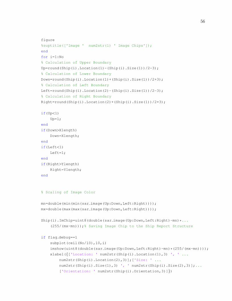
56

figure

%suptitle(['Image ' num2str(1) ' Image Chips']);

end

for i=1:No

% Calculation of Upper Boundary

Up=round(Ship(i).Location(1)-(Ship(i).Size(1))/2-3);

% Calculation of Lower Boundary

Down=round(Ship(i).Location(1)+(Ship(i).Size(1))/2+3);

% Calculation of Left Boundary

Left=round(Ship(i).Location(2)-(Ship(i).Size(1))/2-3);

% Calculation of Right Boundary

Right=round(Ship(i).Location(2)+(Ship(i).Size(1))/2+3);

if(Up<1)

Up=1;

end

if(Down>Xlength)

Down=Xlength;

end

if(Left<1)

Left=1;

end

if(Right>Ylength)

Right=Ylength;

end

% Scaling of Image Color

mn=double(min(min(sar image(Up:Down,Left:Right))));

mx=double(max(max(sar image(Up:Down,Left:Right))));

Ship(i).ImChip=uint8(double(sar image(Up:Down,Left:Right)-mn)*...

(255/(mx-mn)));% Saving Image Chip to the Ship Report Structure

if flag debug==1

subplot(ceil(No/10),10,i)

imshow(uint8(double(sar image(Up:Down,Left:Right)-mn)*(255/(mx-mn))));

xlabel({['Location: ' num2str(Ship(i).Location(1),3) ', ' ...

num2str(Ship(i).Location(2),3)];['Size: ' ...

num2str(Ship(i).Size(1),3) ', ' num2str(Ship(i).Size(2),3)];...

['Orientation: ' num2str(Ship(i).Orientation,3)]})

57

title(['Ship ' num2str(i)])

end

end

end