Shimmy of an Aircraft Main Landing Gear

with Geometric Coupling and Mechanical Freeplay

C. HowcroftDept. Engineering Mathematics, University of Bristol, UK

M. LowenbergDept. Aerospace Engineering, University of Bristol, UK

S. NeildDept. Mechanical Engineering, University of Bristol, UK

B. KrauskopfDept. Mathematics, University of Auckland, New Zealand

E. CoetzeeFuture Projects, Airbus, Filton, UK

March 2014

Abstract

The self-sustained oscillation of aircraft landing gear is an inherently nonlinear and dynamically complexphenomenon. Although such oscillations are ultimately driven from the interaction between the tyres andthe ground, other effects, such as mechanical freeplay and geometric nonlinearity, may influence stabilityand add to the complexity of observed behaviour. This paper presents a bifurcation study of an aircraftmain landing gear, which includes both mechanical freeplay, and significant geometric coupling, the latterachieved via consideration of a typical side-stay orientation. These aspects combine to produce complexoscillatory behaviour within the operating regime of the landing gear, including longitudinal and quasi-periodic shimmy. Moreover, asymmetric forces arising from the geometric orientation produce bifurcationresults that are extremely sensitive to the properties at the freeplay/contact boundary. However thissensitivity is confined to the small amplitude dynamics of the system. This affects the interpretationof the bifurcation results; in particular bifurcations from high amplitude behaviour are found to formboundaries of greater confidence between the regions of different behaviour given uncertainty in thefreeplay characteristics.

1 Introduction

Oscillations of rolling systems (appearing as a wobbling or weaving motion) is a well known problem inengineering. This behaviour represents an undesired characteristic in a wide array of different applications,ranging from castered trolleys, motorcycles and pulled trailers to aircraft landing gear. Such oscillationscan be a consequence of periodic forcing, for example, due to out-of-balance components, or they may arisefrom feedback via the wheel contact dynamics [14]. It is the latter type that we focus on in this work; oftentermed shimmy, these oscillations result from the interplay of structural and tyre contact dynamics, andthey may occur even in well-balanced systems. Aircraft landing gear may prove particularly susceptible to

1

these oscillations. Their structures display numerous flexible modes that couple geometrically and via theelastic tyre dynamics. As a result, a wide range of complex oscillatory behaviour may be observed in aircraftlanding gear. Consequently, shimmy has attracted significant research attention, with landing gear formingthe object of a large proportion of the shimmy literature since the 1930s. However, although shimmy oscil-lations are a well documented phenomenon in aircraft ground dynamics, as Shaw and Balachandran pointout in their review paper [19], these oscillations may also appear in other mechanical systems, for example,in the dynamics of motorcycles [2, 11]. For further information on the extensive research into shimmy seethe overview papers of Dengler et al. [4] and Pritchard [17].

In this work we focus on the dynamic stability of an aircraft dual-wheel main landing gear (MLG) anduse the technique of numerical continuation to perform a bifurcation analysis, exploring its nonlinear dy-namics. We bring together several key concepts from the earlier studies [7, 8] and, in particular, focus onthe the combined effects of mechanical freeplay and geometric coupling. Taken individually, these subjectsformed the basis for the two earlier papers. Here, we consider a system with both a complex geometry anda ‘loose’ torque link assembly as a source of freeplay, hence, assessing the role these effects play when con-sidered in conjunction. We highlight a wealth of additional MLG behaviour that results from the interplaybetween these two dynamic effects and go on to discuss how this also has a bearing on the interpretation ofthe system bifurcation diagram.

In general, freeplay may appear from a multitude of different sources in aircraft landing gear; in partic-ular, it occurs naturally as a result of structural wear. Such mechanical freeplays may account for severalmillimetres of translational play at the wheel axle, as well as rotational play in the yaw degree of freedom [1].The freeplay that we consider here takes the form of a lateral play in the landing gear torque links (a typicalsource of landing gear freeplay) which, via the system geometry, results in a torsional play. In [7] we foundthat freeplay of this form has a significant effect on landing gear stability, and we observed a multitude ofresulting oscillatory phenomena. Furthermore, we also found the characteristics of freeplay to be influentialon the observed behaviour with ‘sharper’ freeplay profiles allowing shimmy oscillations over more typicaloperating conditions. This sensitivity to freeplay is also supported in the literature: [18, 22, 28] are allexamples of studies in which the presence of freeplay is found to be detrimental to landing gear stability,reducing the critical velocity above which shimmy oscillations may occur. As such, the careful monitoringof freeplay tolerances is a standard procedure in the maintenance of landing gear in service.

In addition to mechanical freeplay we also consider in this study the geometric complexity arising froma typical side-stay orientation. In [8] we presented a sensitivity analysis into the effect of side-stay orienta-tion of a landing gear system with similar properties to that treated in [24]. We found the precise orientationof the landing gear geometry to have a significant effect on the dynamics, with longitudinal oscillationsoccurring for typical system geometries. This geometric sensitivity not only highlights the possible dynamiccomplexity of a typical MLG system, but also has a bearing on the modelling of the system. Specifically, wenote that despite there being typically several hundred DoFs in even the lowest order landing gear models,we note that one may capture the occurrence of shimmy oscillations by considering a few choice represen-tative DoFs. For the appearance of shimmy oscillation in a rolling system one, in fact, requires only two: atorsional DoF allowing yaw motion of the wheel and some form of lateral flexibility, either in the structureof the system or via the elastic properties of the tyre itself. This is illustrated by Stepan in [21] where heshows the self-sustained oscillation of a pulled wheel system for the cases in which the wheel is rigid and thekingpin is elastic, and vice-versa.

For an aircraft landing gear system the tyres are flexible and, therefore, shimmy oscillations can conceivablyoccur given only torsional motion of the gear structure, as demonstrated by Somieski in the nose landing gearstudy [20]. Here, like in many nose gear designs, the wheel axle trails the yaw axis of the main strut and so,in fact, this system bears resemblance to the simpler pulled wheel systems that exhibit shimmy. While thesetorsional dynamics are sufficient to highlight the shimmy phenomenon in landing gear systems, in practice,the bending and deflection of the gear structure and main strut introduce extra DoFs to the dynamics of

2

δβ

LβLβ − η

ηLδ

ρ

z

y

z

x

z

x

(a) (b) (c)

torquelinks

side-stay

mainstrut

ψ

V

µ

λR

λL

h

Y

X

x

y(d) (e)

Figure 1: The six degrees of freedom used in characterising the deflected state of the dual-wheel MLGsystem. ψ, δ and β denote angular deflections of the gear structure, and η, λL and λR linear deflectionsof the main strut and tyre contact patches, respectively. Global (X, Y, Z) coordinates are defined relativeto the (X, Y) ground-plane (X forwards, Z up); (x, y, z) are defined locally with z aligned with the mainstrut, x perpendicular to the main strut and side-stay, and y chosen to complete the right-handed coordinatesystem. For the zero rake angle case shown here z = Z.

the landing gear that may couple with these torsional dynamics. Therefore, in general, low-order studies oflanding gear systems consider the presence of additional DoFs to incorporate these effects. In [25] Thota etal. consider the dynamics of a nose landing gear as expressed in terms of the lateral and longitudinal bendingof the main strut, as well as torsional motion of the wheel. The study concludes that, whilst the torsional andlateral dynamics are observed to couple, the longitudinal DoF does not actively participate in the dynamicsof the system. This finding is supported in the work of Van Der Valk and Pacejka [26], where they considerthe dynamic stability of a dual-wheel ‘Fokker F28-like’ main landing gear, neglecting longitudinal deflectionsof the system. It is, however, worth pointing out that for the aircraft design considered in their study theside-stay is mounted laterally, i.e. at 90

to the forward direction of the aircraft. This is not the case for the

study of this paper.

From our previous work in [8], we infer that a description of fore-aft motion of the landing gear is re-quired in capturing the full dynamics of the system with a more complex side-stay geometry. Furthermore,we note that axial compression and extension of the system, also neglected in many studies, forms an im-portant component of the longitudinal dynamics, allowing the appearance of so called gear-walk; this isdiscussed in references [9, 10] and seen later in this paper. Consideration of axial deflection is also required

3

to express the form of freeplay we consider, which varies with landing gear extension [7]. Therefore, althougha number of studies only incorporate torsional and lateral DoFs (examples of which may be seen in references[16, 18, 22, 24]), for this study, we employ the model described in [7] which considers the MLG dynamics interms of four structural, and two tyre DoFs.

This paper is organised as follows. In section 2 we recap the landing gear model. For this model, weset a typical side-stay orientation for a civil aircraft main gear and explore in sections 3 and 4 the dynamicsof the MLG in the presence of zero and non-zero mechanical freeplay, respectively. It is for the non-zerofreeplay case that we observe the greatest complexity of bifurcation results with a marked increase in thevariety of observable dynamics when compared with the results for the lateral side-stay study of [7]. Insection 4.1 we compute one-parameter bifurcation diagrams to show that this complexity arises from thepresence of a longitudinal mode of shimmy oscillation in the dynamics of the system, a consequence of theincreased geometric coupling for a side-stay orientation that is neither purely lateral nor longitudinal withrespect to the direction of travel. We also observe the appearance of multi-frequency oscillations, and theseare explored with numerical continuation and simulation in section 4.2. In section 4.3 we focus on the in-fluence of asymmetry in the system, an aspect of the MLG geometry for a non-lateral side-stay orientation.In particular, we find that certain points of bifurcation associated with low-amplitude behaviour may provevery sensitive to even small changes to the properties and size of freeplay; this is illustrated and discussedin section 4.4. Finally, in section 5 we discuss our findings regarding shimmy instability arising from theinterplay of freeplay, sidestay geometry and axial DoF effects.

2 Main landing gear model

We begin by recapping the basic structure and properties of the main landing gear model from [7]. Theparticular MLG configuration that we consider is of a dual-wheel, single side-stay design; various views ofthis system are illustrated in figure 1. To construct a dynamic model of this MLG amenable to the nonlinearanalysis techniques employed in this study we use a low-order description of its dynamics. To this endwe represent the deflection of both structure and tyres in terms of six DoFs that characterise the systembehaviour. These DoFs, which are displayed in figure 1, are:

1. The torsional DoF: twisting motion ψ of the wheels and axle about the main strut axis. This yawingmotion is resisted by the landing gear torque links (shown only in panel (c)) which lend torsionalstiffness to the system whilst allowing for compression and extension of the landing gear (see section2.1).

2. The in-plane DoF: bending of the lower gear in the side-stay (y,z)-plane (the plane spanned by theside-stay and main strut). This motion is approximated as an angular motion δ with radius Lδ.

3. The out-of-plane DoF: rotation β out of the side-stay (y,z)-plane about the MLG attachment points.The main strut has an inclination (or rake angle) φ0 when β = 0 (for figure 1, φ0 = 0).

4. The axial DoF: compression and extension of the shock absorber, parameterised by η.

5. Two lateral tyre DoFs: lateral tyre deflections taken at the front of the tyre contact patches; here, λLand λR denote deflections of the left and right tyres, respectively.

The mathematical description of this system takes the form of six ordinary differential equations (ODEs),corresponding to each of these DoFs. These equations are written respectively as

4

Iψψ − Ia Ωax Ωay + cψ[ψ + β sin p ] +Mkψ(η) =Mψ(Fdyn) , (1)

Iδ(η, θa)δ + Iaθa cos θa Ωay − Iaθa sin θaΩax

+∂ηIδ(η)ηδ − 1/2∂δIβ(δ, η)β2 + cδ δ + kδδ =Mδ(Fdyn) , (2)

Iβ(δ, η, θa)β + ∂δIβ(δ, η)δβ + ∂ηIβ(δ, η)ηβ

−MHLβ(η)[H1 sinβ −H2 cosβ]

−Ia[θa sin θa Ωay cos p+ θa cos θa Ωax cos p

+ Ωax Ωay sin p ] + cβ β + cψ[ψ + β sin p ] sin p

+kββ +Mkψ(η) sin p =Mβ(Fdyn) , (3)

−MH cosφ− 1/2∂ηIβ(δ, η)β2 − 1/2∂ηIδ(η)δ2

+Fcη(η) + Fkη(η) =Fη(Fdyn) , (4)

λL + [VLCF · uf ]λL/LL(Fdyn) + [V∗LCF · uλ] = 0 , (5)

λR + [VRCF · uf ]λR/LR(Fdyn) + [V∗RCF · uλ] = 0 , (6)

where

Ωax = δ cos θa − β sin θa cos p ,

Ωay = −δ sin θa − β cos θa cos p ,θa = ψ + β sin p+m ,

H = (−H1 sinβ +H2 cosβ)(Lβ β − 2ηβ)

+ (−H1 cosβ −H2 sinβ)Lβ β2 − η cosφ ,

cosφ = H1 cosβ +H2 sinβ +H3 ,

H1 = cosφ0 cos2 ρ+ sinφ0 sin ρ cos ρ sinµ ,

H2 = − sinφ0 cos ρ cosµ ,

H3 = cosφ0 sin2 ρ− sinφ0 sin ρ cos ρ sinµ .

The four structural equations (1)–(4) may be obtained from a Lagrangian approach, minimising the totalsystem energy; note that for clarity we write equation (4) in terms of the vertical gear height H = Lβ cosφ.The damping characteristics of the DoFs ψ, δ and β are represented by the linear coefficients cψ, cδ and cβ ,the stiffness characteristics of the DoFs δ and β by the linear coefficients kδ and kβ . More general expres-sions Fkη, Fcη and Mkψ are used for the axial stiffness, axial damping and torsional stiffness, respectively,which cannot be accurately represented by linear relations. In particular, the resistive forces produced bythe shock absorber are expressed by nonlinear functions fitted to industrial data, and the torsional stiffnessof the system depends upon the geometry of the torque links and, as such, varies with the gear compressionη. The parameters Iψ, Iδ, Iβ denote the inertias of their respective DoFs, Ia is the roll inertia of the wheelsand axle, and M is the modal mass associated with vertical movement of the aircraft. Mψ, Mδ, Mβ and Fηexpress external forces (consisting of loading, gyroscopic and tyre reaction forces) resolved into each of thefour DoFs. For full details see [7] or the extended discussion in [6].

The geometric angle φ gives the rake angle of the main strut (see figure 2); for β = 0, the initial rakeangle of the strut is φ0. The angles ρ and µ describe the orientation of the side stay in the global (X,Y, Z)coordinate system see figure 1. Specifically, if one considers the vector running from the main strut attach-ment point to the side-stay attachment point, its orientation from an initial position parallel to the lateral Y

5

p

m

φ

V

.

.

Figure 2: Depiction of the side-stay angles m, p, and the MLG rake angle φ; for the landing gear of thisstudy (m, p, φ) = (40, 0,−7)

.

axis may be defined by a rotation ρ about the forward X axis, followed by a rotation µ about the vertical Zaxis. In addition, the orientation of this chord may be expressed by the angles m and p instead defining theorientation with respect to the main strut (fig: 2). The relation between (m, p) and (µ, ρ) may be writtenas:

p = sin−1( cosφ0 sin ρ− sinφ0 cos ρ sinµ) ,

m = sin−1((sinφ0 sin ρ+ cosφ0 cos ρ sinµ)/ cos p) .

Using this description of the side-stay orientation, orthogonality between the main strut and attachmentpoint chord is given by the condition p = 0.

Equations (5)–(6) represent the tyre dynamics of the MLG system. These equations are obtained viaadaptation of the von Schlippe tyre model [27] wherein the deflected shape of each tyre is represented by astretched string. The specific shape of this stretched string profile may be characterised based on the lateraldeflections λL and λR at the front of the contact patches. Here, LL and LR denote the relaxation coefficientsof each tyre and uf and uλ are unit vectors aligned in the forward and lateral directions with respect tothe direction in which the wheel axle is pointing. The terms VLCF and VRCF denote the velocity vectors ofthe left and right wheels in the global coordinate system, relative to the ground (e.g. ViCF = [50, 0, 0] for astraight-rolling wheel with forward speed of 50 m/s). The expressions V ∗

LCF and V ∗RCF are modifications to

these vectors; they neglect the effects of torsional ψ motion and, for the MLG system considered, improvethe accuracy of the tyre model for short wavelength oscillation [7]. Further information on all of these terms,as well as the specific application of the von Schlippe model to this system, may be found in reference [7].

An important aspect of this model is that a number of parameters of the landing gear vary with the loadingforce acting through the landing gear. In equations (1)–(6) we highlight these parameters as functions ofthe dynamic loading force Fdyn = MH + Fz, where Fz is the applied external loading and H describes thevertical height of the gear. Since this dynamic loading varies with the vertical acceleration of the system,the axial DoF η, can prove particularly influential on the loading forces and the parameters on which thisloading depends. In addition there are a number of parameters in the model that depend directly on thegear length and are therefore functions of the deflection η; these are also highlighted in the equations ofmotion. This variation reinforces the importance of considering axial motion of the MLG system. We willsee that compression and extension of the MLG later goes on to play an important role in the occurrence of

6

0 0.1201 0.2402 0.3603−0.1201−0.2402−0.3603−5

−4

−3

−2

−1

0

1

2

3

4

5x 10

4 −1 1

ψ (deg)

Mkψ(N

m)

ytlk

(mm)

rtlk(η)

ψfp(η)

yfp

ytlk

2ǫ

(a) (b)

Figure 3: Panel (a) is a depiction of the landing gear torque link geometry. Here an apex freeplay of yfp

mm translates into a torsional freeplay of ψ

fp. Panel (b) shows an example moment, deflection profile of the

ψ-DoF for F ∗z = 1.0 (giving r

tlk= 0.477 m) and ε = 0.1 mm.

gear walk. Once again we direct the reader to [7] for the specific expressions pertaining to the variation ofthese parameter values with loading and gear extension.

2.1 Freeplay model

As a final point, we recap the considered representation of freeplay of the MLG system, which arises froma lateral play in the apex of the torque links. As mentioned in section 1, freeplay naturally develops inthe mechanical joints of any real system due to wear. In the case of torque link freeplay, this can havea particularly significant effect on the torsional stability of the system and the subsequent occurrence oftorsional shimmy [18, 22, 28]. Therefore consideration of shimmy stability of a landing gear may imposelimits on the maximum allowable freeplay and therefore influence the maintenance requirements for thesystem. The placement of the MLG torque links in relation to the MLG structure is shown in panel (c) offigure 1; a more detailed view of the torque link geometry is given in figure 3(a). Due to this configuration,separation of the torque links will result in a range of yaw angles ψ ∈ (−ψ

fp, ψ

fp) over which the landing

gear will experience a greatly reduced torsional stiffness. The magnitude of this yaw freeplay will vary withaxial η deflection as the radial distance between torque link apex and yaw centre line r

tlkvaries. An example

force-deflection profile representing the stiffness properties of the torsional DoF for 1mm of freeplay is shownin panel (b) of figure 3. The specific form of this profile is given by

Mkψ = ktlk

1

π

((y

tlk+ y

fp)[

tan−1(− (y

tlk+ y

fp)/ε)

+π

2

]+(y

tlk− y

fp)[

tan−1(

+ (ytlk− y

fp)/ε)

+π

2

])rtlk . (7)

As discussed in [7], we introduce a degree of smoothing here to reflect the fact that, for any real system, thetransition from freeplay to contact is unlikely to be truly non-smooth. Using the above form for the stiffnessprofile this transition roughly spans the range 2ε. For this study we consider both the MLG system withoutfreeplay as well as the MLG system with ± 1mm of lateral play at the torque link apex. We initially set thesmoothing parameter ε to 0.1 mm.

7

0 100 200 300 400 500 6000

2

4

6

8

10

12

14

16

18

20

V (m/s)

Maxψ

(deg)

stable

unstable

Figure 4: One-parameter bifurcation diagram in V for the MLG system defined by equations (1)–(7) withzero freeplay and fixed F ∗

z = 1.

V (m/s)

H

no shimmy shimmy

F∗ z

Figure 5: Two-parameter bifurcation diagram of the MLG system (1)–(7) with zero torque link freeplay.The region enclosed by the dashed line indicates a typical operating envelope of the MLG.

3 Zero freeplay system

We focus first on the MLG as expressed by equations (1)–(7), without torque link freeplay, that is for yfp

= 0mm. Parameter values are set in accordance with [7] and serve to represent a typical mid-range civil MLG(physically larger in size and stiffness than that considered in [8]). In addition, we assign a side-stay orien-tation angle of µ = 40

to reflect the configuration of a typical civil aircraft. We also note that for many

MLGs of this design (see figure 1), the side-stay attachment point is locked beneath that of the main strut.Here we set the horizontal inclination parameter ρ = tan−1(tanφ0 sinµ) = −4.513

which in turn implies

that the attachment point inclination relative to the main strut is p = 0.

A numerical continuation methodology is employed throughout this study to construct bifurcation diagramsof the MLG and so characterise the observable behaviour of this system. The bifurcation parameters on whichwe focus are the forward velocity V of the system and the applied normalised loading force F ∗

z (which denotesthe loading force acting on the landing gear as a proportion of the nominal loading with zero lift). Both areexamples of operational parameters that vary substantially during any particular landing or take-off scenario.

8

We first present a one-parameter bifurcation diagram of this system, as shown in figure 4, focusing onvariation of the forward velocity. Curves in this diagram signify solutions of the system in terms of theirmaximum amplitude in ψ. The stability of these solutions is also indicated. We see here that over theentire velocity range considered there exists a zero amplitude solution corresponding to straight-rolling be-haviour of the MLG. This solution is stable over all likely operating velocities of the system. However, wenote that for extreme forward velocities this solution is observed to lose stability at a super-critical Hopfbifurcation point beyond which a branch of stable limit cycle oscillations exists. This Hopf bifurcation pointtherefore indicates the critical velocity beyond which shimmy oscillations will occur. We note that, althoughthis critical velocity is well beyond the operating velocity of the main landing gear system, its value mayalso depend on additional parameters, the variation of which may bring this velocity to within the MLGoperating envelope. The loading force F ∗

z is an example of a parameter on which this critical velocity depends.

With the numerical continuation software AUTO we are able to track the location of this characterisingHopf bifurcation point as the loading force acting on the system is varied. Doing so produces the two-parameter bifurcation diagram, shown in figure 5, where we see a single Hopf bifurcation curve in the(V ,F ∗

z )-plane. As reflected in the one-parameter result of figure 4, we see that to the left of this curve theMLG is stable, whilst to the right the landing gear will experience shimmy. Despite the sensitivity of thiscurve to the variation of loading force we note that this region of shimmy instability still does not occur overtypical operating conditions; an example operational envelope is indicated by the dashed line.

Another feature of the two-parameter diagram of figure 5 is a second Hopf bifurcation curve for very smallF ∗z at the bottom of the plot (see enlargement in figure 5) which bounds a very small region of torsional os-

cillations. These oscillations have low amplitude and frequency and so incur little stress on the landing gearwhen compared with the shaded torsional shimmy region. Moreover, since this region only exists for verylight aircraft loads (F ∗

z < 0.02), in practice, the conditions on the landing gear will pass rapidly through thisregion during touch-down and take-off procedures of the aircraft, leaving insufficient time for the transientdynamics to settle into significant oscillation of the system. We therefore reason that, despite lying withinthe operational envelope of the MLG, these oscillations are acceptable in practice, having little effect onthe dynamics, particularly when considered alongside large perturbations of the MLG during take-off andlanding.

4 Non-zero freeplay

Overall, we see from figure 5 that despite the sensitivity to side-stay geometry observed in our previous study[8], the larger and stiffer system of this study displays relatively simple dynamic behaviour for the typicalside-stay orientation of µ = 40

considered here. With this result in mind, we next examine the behaviour of

the system under the influence of torque link freeplay. We choose a freeplay of ±1 mm at the torque link apexand set ε = 0.1 mm, which corresponds to a smoothing region of one fifth of the freeplay width. As discussedin section 2.1, a truly non-smooth transition from freeplay to contact is unlikely to occur in a physical systemand rather a finite transition region is to be expected. The addition of this freeplay to the torque links ofthe MLG results in the two-parameter bifurcation diagram shown in figure 6; for clarity we show here onlythe bifurcation curves pertinent to the dynamics, neglecting those that do not specifically bound regionsof different observable behaviours. We immediately note a greatly increased complexity of behaviour whencompared to the result of figure 5. We find curves of Hopf bifurcation, of saddle-node (or fold) bifurcation, oftorus bifurcation, and of period-doubling bifurcation; curve-types corresponding to each of these bifurcationsare labelled in the figure. New features for the freeplay case include a large region of high-frequency shimmyoscillation bounded by a single fold curve, as well as additional regions of ‘gentler’ shimmy oscillation (givenby the wider shading). Oscillations in these latter regions, although still representing self-sustaining shimmy,are of small amplitude and low frequency and, therefore, do not exert the same levels of stress on the landinggear structure as do the high frequency oscillations. Importantly, both gentle and high-frequency shimmy

9

.

V (m/s)

F∗ z Hx

Hopf

Saddle-node

Period-doubling

Torus .

no shimmy torsional shimmy low frequency shimmy

Figure 6: Two-parameter bifurcation diagram of the MLG system for ±1 mm of torque link freeplay.

regions now intersect the operational envelope of the MLG system and so may be observed under operation.A further feature of importance in the bifurcation diagram of figure 6 is the appearance of curves of torusand period doubling bifurcations. Along with co-dimension two double Hopf bifurcation points they indicatethe appearance of new frequencies and types of oscillation in the dynamics of the system. To further explorethese features we now consider a number of representative one-parameter bifurcation diagrams, where theforward velocity V is again the bifurcation parameter and the loading force F ∗

z is held fixed.

10

0 20 40 60 80 100 120 140 160 180 200−0.3

−0.2

−0.1

0

0.1

0.2

0.3

V (m/s)

ψ(deg)

0 20 40 60 80 100 120 140 160 180 200

0.316

0.318

0.32

0.322

0.324

0.326

0.328

V (m/s)

xgro

und(m

)

0 20 40 60 80 100 120 140 160 180 2000

5

10

15

20

25

30

V (m/s)

Frequen

cy(H

z)

(a)

(b)

(c)

Hx

Hx

Hopf bifurcationSaddle-node bifurcation

Torus bifurcationPeriod-doubling bifurcation.

Figure 7: One-parameter bifurcation diagram in V with F ∗z = 1 and y

fp= 1 mm. The minimum and

maximum amplitude of solutions are expressed in ψ (a) and xground (b), while panel (c) shows their frequency.Points of bifurcation along these curves are as indicated in the key in panel (a).

11

4.1 One-parameter bifurcation diagrams

Figure 7 shows the one-parameter bifurcation diagram with freeplay for F ∗z = 1. The diagram consists of

both oscillatory and stationary solution curves. Bifurcation points along these curves are as indicated in thekey. Panel (a) shows the ψ-amplitude of solutions, panel (b) their ground deflection xground = −Lβ sinφ ,and panel (c) their frequency. We note that the geometric asymmetry of the system for non-zero µ, coupledwith the weak restoring forces about ψ = 0 within the freeplay region, results in limit cycle oscillations thatare largely asymmetric, particularly over small amplitudes. Therefore, we indicate both the maximum andminimum amplitude of periodic solution curves to better reflect the shape of oscillation. The stationarysolution (ψ = 0.102

) which exists over the entire velocity range considered, is stable over the operating

region V ∈ [0, 80] and bifurcates at two Hopf bifurcation points at V = 110.5 m/s and V = 142.7 m/s. Thefirst of these at V = 110.5 is supercritical. Starting to the left of this bifurcation we observe, with increasingV , a loss of stability of the stationary solution and the creation of a branch of stable periodic solutions.However, this branch immediately loses stability at a torus bifurcation point. Continuing along this solutioncurve we see that the torsional amplitude of oscillation increases with the branch remaining unstable upuntil the saddle-node bifurcation at V = 42.5. Here the solution branch folds back on itself and regainsstability, thus resulting in a stable branch of shimmy oscillations for V > 42.5. These oscillations start atjust over 15 Hz — see figure 7(c) — and increase in frequency as the ψ-amplitude of the periodic solutionbranch continues to increase. A similar variation in frequency was also observed in [7], and is a consequenceof the decreasing influence of the freeplay region for larger torsional amplitudes [22]. The existence of thisbranch of torsional shimmy oscillations together with the stable stationary solution gives rise to multiple-stability between solutions in the dynamics of the system. Specifically, for forward velocities in the rangeV ∈ [42.5, 110.5] the system may experience either oscillatory or straight-rolling behaviour; in the presenceof external perturbing forces the MLG system is capable of moving between these solutions.

We now focus on the second Hopf bifurcation point labelled Hx in figure 7; the corresponding bifurcationcurve is also labelled in figure 6. We find that, unlike the other Hopf bifurcation curves in this two-parameterbifurcation diagram, the curve Hx does not result from a shift in the curves shown in figure 4 as freeplayis introduced into the system. Rather the curve Hx originates outside of the (V, F ∗

z ) range considered. In[8] we found that an increased dynamic complexity for intermediate sidestay orientations was accompaniedby the appearance of additional Hopf bifurcation curves which marked the entry of longitudinal oscillationsinto the behaviour of the system. We observe here that the additional point Hx signifies a similar appear-ance of longitudinal behaviour in the MLG system. We note, however, that for the MLG of this study,the β and η DoFs are strongly coupled, both acting to produce variations in gear height H. Therefore,the appearance of longitudinal-type oscillations in the MLG must be expected to incorporate both β andη motion. To illustrate this we present in figure 7(b) the projection of the one-parameter solution curvesin terms of the resulting ground deflection xground(β, η) = −Lβ sinφ (recall for this system, the rake angleφ is negative). We see here that the solution branch created at Hx has a comparatively high amplitudein panel (b) and low amplitude in panel (a) when compared with the first solution branch. This indicatesthat shimmy oscillations along this branch display a walking-type motion of the gear associated with a highxground amplitude. Looking to figure 7(c) we find that these oscillations have a lower frequency and, unlikethe first curve, this frequency does not change significantly as the forward speed V (and torsional ampli-tude) of the solution varies. Furthermore, for velocities beyond the range depicted in figure 7, the torsionalcomponent of this solution curve grows to exceed the freeplay width (ψ

fp∈ (0.07, 0.13)) with limit cycles

intersecting the contact region; however despite this, the oscillation frequency of this branch still remains ataround the same value. This is significant because it indicates an insensitivity of the oscillations bifurcatingat Hx to the changing torsional stiffness of the gear over the freeplay/contact regions. This is in contrast tothe torsional shimmy oscillations observed thus far which prove sensitive to the torque link stiffness profile.Therefore these results provide further evidence to support the appearance of an additional, non-torsionaltype of shimmy oscillation.

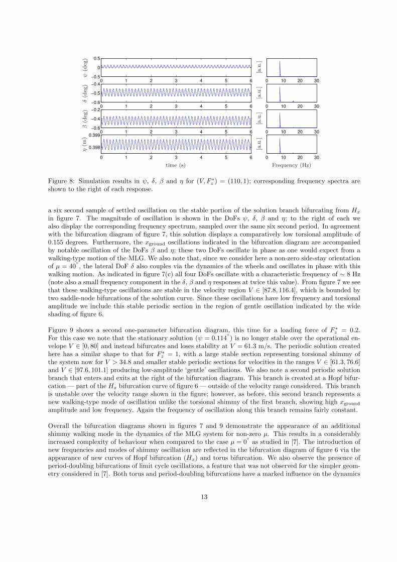
An example of this walking motion is illustrated in the time series of figure 8. Here we show, for V = 110 m/s,

12

0 10 20 30

0 10 20 30

0 10 20 30

0 10 20 30

0 1 2 3 4 5 6−0.5

0

0.5

0 1 2 3 4 5 6−0.6

−0.5

−0.4

0 1 2 3 4 5 6−0.6

−0.4

−0.2

0 1 2 3 4 5 6

0.398

0.399

time (s) Frequency (Hz)

ψ(deg)

δ(deg)

β(deg)

η(m

)

[a.u.]

[a.u.]

[a.u.]

[a.u.]

Figure 8: Simulation results in ψ, δ, β and η for (V, F ∗z ) = (110, 1); corresponding frequency spectra are

shown to the right of each response.

a six second sample of settled oscillation on the stable portion of the solution branch bifurcating from Hx

in figure 7. The magnitude of oscillation is shown in the DoFs ψ, δ, β and η; to the right of each wealso display the corresponding frequency spectrum, sampled over the same six second period. In agreementwith the bifurcation diagram of figure 7, this solution displays a comparatively low torsional amplitude of0.155 degrees. Furthermore, the xground oscillations indicated in the bifurcation diagram are accompaniedby notable oscillation of the DoFs β and η; these two DoFs oscillate in phase as one would expect from awalking-type motion of the MLG. We also note that, since we consider here a non-zero side-stay orientationof µ = 40

, the lateral DoF δ also couples via the dynamics of the wheels and oscillates in phase with this

walking motion. As indicated in figure 7(c) all four DoFs oscillate with a characteristic frequency of ∼ 8 Hz(note also a small frequency component in the δ, β and η responses at twice this value). From figure 7 we seethat these walking-type oscillations are stable in the velocity region V ∈ [87.8, 116.4], which is bounded bytwo saddle-node bifurcations of the solution curve. Since these oscillations have low frequency and torsionalamplitude we include this stable periodic section in the region of gentle oscillation indicated by the wideshading of figure 6.

Figure 9 shows a second one-parameter bifurcation diagram, this time for a loading force of F ∗z = 0.2.

For this case we note that the stationary solution (ψ = 0.114) is no longer stable over the operational en-

velope V ∈ [0, 80] and instead bifurcates and loses stability at V = 61.3 m/s. The periodic solution createdhere has a similar shape to that for F ∗

z = 1, with a large stable section representing torsional shimmy ofthe system now for V > 34.8 and smaller stable periodic sections for velocities in the ranges V ∈ [61.3, 76.6]and V ∈ [97.6, 101.1] producing low-amplitude ‘gentle’ oscillations. We also note a second periodic solutionbranch that enters and exits at the right of the bifurcation diagram. This branch is created at a Hopf bifur-cation — part of the Hx bifurcation curve of figure 6 — outside of the velocity range considered. This branchis unstable over the velocity range shown in the figure; however, as before, this second branch represents anew walking-type mode of oscillation unlike the torsional shimmy of the first branch, showing high xgroundamplitude and low frequency. Again the frequency of oscillation along this branch remains fairly constant.

Overall the bifurcation diagrams shown in figures 7 and 9 demonstrate the appearance of an additionalshimmy walking mode in the dynamics of the MLG system for non-zero µ. This results in a considerablyincreased complexity of behaviour when compared to the case µ = 0

as studied in [7]. The introduction of

new frequencies and modes of shimmy oscillation are reflected in the bifurcation diagram of figure 6 via theappearance of new curves of Hopf bifurcation (Hx) and torus bifurcation. We also observe the presence ofperiod-doubling bifurcations of limit cycle oscillations, a feature that was not observed for the simpler geom-etry considered in [7]. Both torus and period-doubling bifurcations have a marked influence on the dynamics

13

0 20 40 60 80 100 120 140 160 180 200−0.5

−0.4

−0.3

−0.2

−0.1

0

0.1

0.2

0.3

0.4

0.5

V (m/s)

ψ(deg)

0 20 40 60 80 100 120 140 160 180 2000.326

0.327

0.328

0.329

0.33

0.331

0.332

0.333

0.334

V (m/s)

xgro

und(m

)

0 20 40 60 80 100 120 140 160 180 2000

5

10

15

20

25

30

V (m/s)

Frequen

cy(H

z)(a)

(b)

(c)

Figure 9: One-parameter bifurcation diagram in V for F ∗z = 0.2 and y

fp= 1 mm. The minimum and

maximum amplitude of solutions are expressed in ψ (a), xground (b), and frequency (c).

14

of the system, leading to the creation of higher-period and quasi-periodic oscillations. Such phenomena havealso been observed in the studies of other physical systems prone to shimmy instability [23].

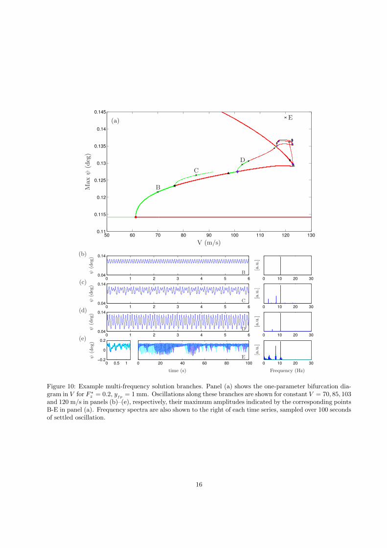
4.2 Multiple-frequency oscillation

To illustrate the influence of the torus and period-doubling bifurcations we again focus on the dynamics of thesystem for a loading force of F ∗

z = 0.2; see the one-parameter bifurcation diagram in figure 10(a). For claritywe now consider only the maximum ψ-amplitude of solution curves; in addition to the periodic solutionbranches indicated previously, we also show period-doubled solution branches. These bifurcate in a sequenceof period-doubling bifurcations starting at V = 101.1 as shown. Along with the torus bifurcations presentin the system, this results in a rich variety of observable dynamics. In a series of four numerical simulationsin panels (b)–(e) of figure 10 we highlight, for F ∗

z = 0.2 and constant V , examples of the behaviour thatmay be observed over the parameter range shown. In each case we show both a simulated time series in ψcovering 6 seconds of the settled response, as well as the corresponding frequency spectrum sampled over100 seconds; this longer sampling period is necessary to obtain precise locations of the dominant frequenciesin the response. The maximum amplitudes of each example oscillation are also marked by the points B-Eon the bifurcation diagram of figure 10(a).Figure 10(b) shows the time series in ψ for a forward velocity of V = 70 m/s. We observe that theseoscillations are periodic with a single dominant frequency of 10.56 Hz. This oscillation is marked as pointB in panel (a), and we observe that this periodic orbit constitutes periodic motion on the stable oscillatorybranch that bifurcates from the stationary solution at V = 61.3. For a forward velocity of 85 m/s consideredin panel (c) we see a different response. Here we observe motion in ψ that appears quasi-periodic in naturewith multiple frequencies of oscillation of 2.94, 7.71 and 10.64 Hz. Looking to figure 10(a) we note thecorresponding maximum amplitude point C lies above an unstable section of the periodic solution curve,which is bounded by the torus bifurcations at V = 76.6 and V = 97.6. Given the nature of oscillationobserved in panel (c) it is likely that this point is part of a curve of invariant tori bifurcating from a nearbytorus bifurcation. However, such curves of tori cannot be continued directly. Therefore, to track this curvewe performed a series of numerical integrations while incrementing V , storing the maximum amplitude ofthe settled response in each case. The result is shown in figure 10(a), where a polynomial curve has beenfitted through the obtained points. In this way, an approximation of the attracting branch of multi-frequencyoscillations is obtained on which the observed dynamics of panel (c) lie. We see that, when tracked in thenegative V direction, this branch is found to emerge from the nearby torus bifurcation at V = 76.6.Another type of multiple-frequency solution is observed in figure 10(d) for a forward velocity of 103 m/s.Here the observed periodic orbit is characterised as having two dominant frequencies 5.264 and 10.528 Hz,one precisely double the other. We see that this oscillation (point D) lies on the period-doubled solutionbranch that bifurcates from the simple oscillatory solution at V = 101.1; see panel (a). This branch canbe continued numerically and we find that it is, in fact, one in a series of period-doubled branches. Eachperiod-doubling sees an increased complexity of the observed behaviour and this brings us to the simulatedcase for a forward velocity of 120 m/s shown in figure 10(e). This response shows considerable complexityand we present a longer time series of 100 seconds to capture the behaviour. We see that here the underlyingstructure of oscillation is very hard to discern by inspection as it shows no repetition over the time rangeconsidered. The light curves plotted in the background of panel (e) indicate the simulated response of thesystem given the same parameter values but with initial conditions truncated to seven significant figures.From the leftmost plot of panel (e) showing the first 1.2 seconds of simulation we see that this responsequickly diverges from the dark curve and remains distinct for the remainder of the simulated time frame.Therefore, these MLG oscillations display elements of chaotic motion, including a sensitive dependence onthe choice of initial condition. Looking at the frequency spectrum sampled over the same 100 seconds weobserve that, despite the differences between these responses, they represent the same limiting behaviourhaving near identical frequency components. In particular, they show multiple frequencies of oscillationsthat are less sharply defined than in the cases of panels (b) to (d). Again we show the maximal amplitudepoint, labelled E, in panel (a) and see that for this velocity all local solutions are unstable with the pointlying above these curves.

15

50 60 70 80 90 100 110 120 1300.11

0.115

0.12

0.125

0.13

0.135

0.14

0.145

V (m/s)

Maxψ

(deg)

(a)

B

C

D

E

0 1 2 3 4 5 60.04

0.14

0 10 20 30

0 1 2 3 4 5 60.04

0.14

0 10 20 30

0 1 2 3 4 5 60.04

0.14

0 10 20 30

0 10 20 300 20 40 60 80 1000 0.5 1−0.2

0

0.2

time (s) Frequency (Hz)

ψ(deg)

ψ(deg)

ψ(deg)

ψ(deg)

[a.u.]

[a.u.]

[a.u.]

[a.u.]

(b)

(c)

(d)

(e)

B

C

D

E

Figure 10: Example multi-frequency solution branches. Panel (a) shows the one-parameter bifurcation dia-gram in V for F ∗

z = 0.2, yfp

= 1 mm. Oscillations along these branches are shown for constant V = 70, 85, 103and 120 m/s in panels (b)–(e), respectively, their maximum amplitudes indicated by the corresponding pointsB-E in panel (a). Frequency spectra are also shown to the right of each time series, sampled over 100 secondsof settled oscillation.

16

0 200 400 600 800 1000 1200−0.2

0

0.2

114 115 116 117 118 119 120 121 122 123

0.134

0.136

0.138

0.14

0.142

0.144

0 1 2 3 4 5 6−0.2

0

0.2

0 10 20 30

V (m/s)

time (s)

time (s) Frequency (Hz)

ψ(deg)

ψ(deg)

Maxψ

(deg)

[a.u.]

(a)

(b)

(c)

Es

Es

Figure 11: Additional isolated periodic solution branch for F ∗z = 0.2, y

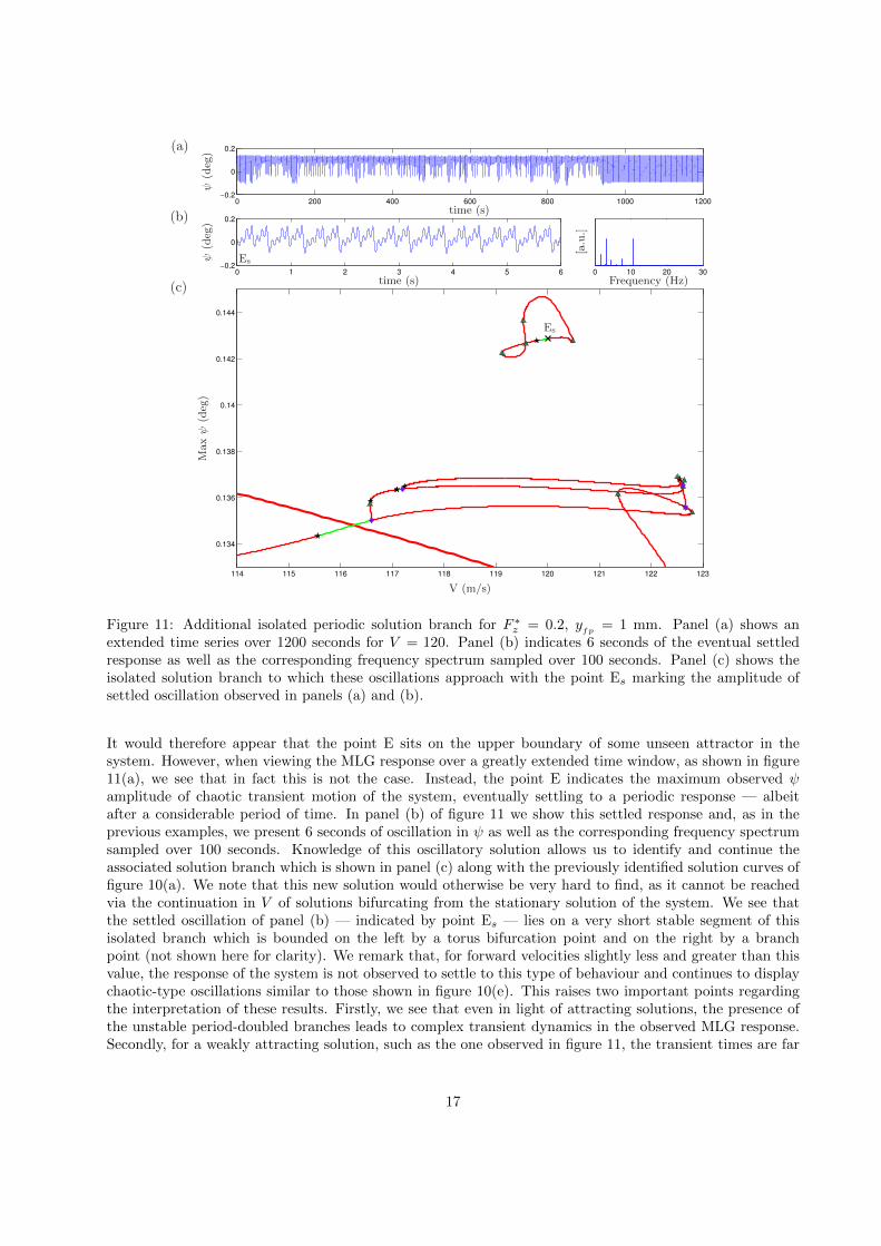
fp= 1 mm. Panel (a) shows an

extended time series over 1200 seconds for V = 120. Panel (b) indicates 6 seconds of the eventual settledresponse as well as the corresponding frequency spectrum sampled over 100 seconds. Panel (c) shows theisolated solution branch to which these oscillations approach with the point Es marking the amplitude ofsettled oscillation observed in panels (a) and (b).

It would therefore appear that the point E sits on the upper boundary of some unseen attractor in thesystem. However, when viewing the MLG response over a greatly extended time window, as shown in figure11(a), we see that in fact this is not the case. Instead, the point E indicates the maximum observed ψamplitude of chaotic transient motion of the system, eventually settling to a periodic response — albeitafter a considerable period of time. In panel (b) of figure 11 we show this settled response and, as in theprevious examples, we present 6 seconds of oscillation in ψ as well as the corresponding frequency spectrumsampled over 100 seconds. Knowledge of this oscillatory solution allows us to identify and continue theassociated solution branch which is shown in panel (c) along with the previously identified solution curves offigure 10(a). We note that this new solution would otherwise be very hard to find, as it cannot be reachedvia the continuation in V of solutions bifurcating from the stationary solution of the system. We see thatthe settled oscillation of panel (b) — indicated by point Es — lies on a very short stable segment of thisisolated branch which is bounded on the left by a torus bifurcation point and on the right by a branchpoint (not shown here for clarity). We remark that, for forward velocities slightly less and greater than thisvalue, the response of the system is not observed to settle to this type of behaviour and continues to displaychaotic-type oscillations similar to those shown in figure 10(e). This raises two important points regardingthe interpretation of these results. Firstly, we see that even in light of attracting solutions, the presence ofthe unstable period-doubled branches leads to complex transient dynamics in the observed MLG response.Secondly, for a weakly attracting solution, such as the one observed in figure 11, the transient times are far

17

0 0.2 0.4 0.6 0.8 1 1.2 1.4 1.6 1.8 2−0.4

−0.3

−0.2

−0.1

0

0.1

0.2

0.3

0.4

F ∗z

ψ(deg)

Figure 12: One-parameter diagram for ε = 0.1 mm and a freeplay of ±1 mm. F ∗z is the bifurcation parameter

and V is fixed at 50 m/s. The boundary of torsional freeplay is indicated by the dashed grey curve.

in excess of the time frame in which the aircraft would remain in the associated (V, F ∗z ) domain. Therefore,

despite the existence of periodic behaviour, in practice one would only observe the more complex transientbehaviour of figure 10(e).

As a final note we remark that apart from the variety of behaviour observed in figures 10 and 11, therealso exists a branch of stable high-frequency torsional shimmy oscillations for V > 34.8 outside of the regionshown; see figure 9. As in the cases of multi-stability observed thus far, a sufficient adverse perturbation ofthe system within this range may move the dynamics from one of these solutions to the other. For the caseof F ∗

z = 0.2 considered here this gives a rich variety of coexisting dynamics between which the system maymove, including stationary, periodic, quasi-periodic, chaotic-type oscillation and higher-frequency torsionalshimmy. It is therefore clear from the results of figures 10 and 11 that the presence of additional curvesof torus and period-doubling bifurcation has a profound influence on the MLG dynamics and represents amechanism through which additional complexity enters the system for non-zero µ.

4.3 Asymmetric effects

We now consider the loading force as a bifurcation parameter and construct the one-parameter bifurcationdiagram in F ∗

z . This is shown in figure 12 for a fixed forward velocity of V = 50 m/s. Solution curvesand points of bifurcation are indicated as in figures 7 and 9; in addition we also show the upper and lowerboundaries of torsional freeplay as dashed grey curves (recall that these vary with the applied loading force;see section 2.1).

Here we see a stable oscillatory branch spanning the entire loading range. This represents torsional shimmyof the system, and is separated from stationary rolling by an unstable section of the same branch. Non-oscillatory behaviour consists of a single stationary solution that is non-zero over the entire F ∗

z -range. Wenote here that this result is different to that observed for the µ = 0

study of [7], where stationary behaviour

consisted of a pitchfork structure with two symmetric non-zero stationary solutions bifurcating from a ψ = 0solution. Hence, for the case µ = 40

, symmetry about ψ = 0 is lost, which is a result of the asymmetric

geometry of the system for non-zero µ. We remark that, in practice, such behaviour is in fact typical of aMLG system: any real system is unlikely to be truly symmetric, even for µ = 0

. In particular, the left

and right tyres will not have precisely equal properties: even well balanced MLG will have slightly differ-ent inflation pressures, stiffness, and response characteristics between the wheels. Furthermore, asymmetricspin-up conditions will result in different temperature distributions in each tyre carcass, in turn affecting anumber of performance parameters [12, 13, 15]. Finally, all pneumatic tyres, including modern aircraft radial

18

0 0.2 0.4 0.6 0.8 1 1.2 1.4 1.6 1.8 20

0.02

0.04

0.06

0.08

0.1

0.12

0.14

0.16

0.18

0.2

F ∗z

ψ(deg)

Figure 13: One-parameter bifurcation diagram in F ∗z showing the MLG stationary solution (solid line) for a

non-smooth freeplay of ±1 mm. The boundary of torsional freeplay is shown by the dashed grey curve. Theblack dash-dot line indicates the boundaries of the loading range over which the stationary solution rests upagainst the boundary of torsional freeplay.

designs, produce a lateral force to one side even at zero slip due to effects such as ply-steer and conicity[3, 5]. These result from the asymmetric composite construction of the tyre carcass. Although dual tyresmay be mounted so that these forces cancel to a certain degree, effects such as ply-steer retain a constantdirection irrespective of which way round the tyre is mounted on the wheel rim. Therefore, in practice, itis very difficult, if not impossible, to fully cancel these lateral forces. Altogether, the effects detailed hereproduce forces asymmetric about zero ψ. Given the light restoring stiffness experienced within the freeplayregion, these have a tendency to move the yaw angle of the wheel axle to the upper or lower boundaries oftorsional freeplay.

4.4 Low-amplitude sensitivity to freeplay smoothing

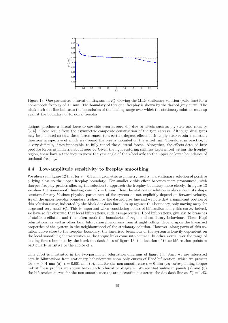
We observe in figure 12 that for ε = 0.1 mm, geometric asymmetry results in a stationary solution of positiveψ lying close to the upper freeplay boundary. For smaller ε this effect becomes more pronounced, withsharper freeplay profiles allowing the solution to approach the freeplay boundary more closely. In figure 13we show the non-smooth limiting case of ε = 0 mm. Here the stationary solution is also shown, its shapeconstant for any V since physical parameters of the system do not explicitly depend on forward velocity.Again the upper freeplay boundary is shown by the dashed grey line and we note that a significant portion ofthis solution curve, indicated by the black dot-dash lines, lies up against this boundary, only moving away forlarge and very small F ∗

z . This is important when considering points of bifurcation along this curve. Indeed,we have so far observed that local bifurcations, such as supercritical Hopf bifurcations, give rise to branchesof stable oscillation and thus often mark the boundaries of regions of oscillatory behaviour. These Hopfbifurcations, as well as other local bifurcation phenomena from straight rolling, depend upon the linearisedproperties of the system in the neighbourhood of the stationary solution. However, along parts of this so-lution curve close to the freeplay boundary, the linearised behaviour of the system is heavily dependent onthe local smoothing characteristics as the torque links come into contact. In other words, over the range ofloading forces bounded by the black dot-dash lines of figure 13, the location of these bifurcation points isparticularly sensitive to the choice of ε.

This effect is illustrated in the two-parameter bifurcation diagrams of figure 14. Since we are interestedhere in bifurcations from stationary behaviour we show only curves of Hopf bifurcation, which we presentfor ε = 0.01 mm (a), ε = 0.001 mm (b), and for the non-smooth case ε = 0 mm (c); corresponding torquelink stiffness profiles are shown below each bifurcation diagram. We see that unlike in panels (a) and (b)the bifurcation curves for the non-smooth case (c) are discontinuous across the dot-dash line at F ∗

z = 1.43.

19

0 200 400 6000

0.2

0.4

0.6

0.8

1

1.2

1.4

1.6

1.8

2

0 200 400 6000

0.2

0.4

0.6

0.8

1

1.2

1.4

1.6

1.8

2

0 200 400 6000

0.2

0.4

0.6

0.8

1

1.2

1.4

1.6

1.8

2

−2 −1 0 1 2−4

−2

0

2

4x 10

4

−2 −1 0 1 2−4

−2

0

2

4x 10

4

−2 −1 0 1 2−4

−2

0

2

4x 10

4

0.99 1 1.01 0.99 1 1.01 0.99 1 1.01

V (m/s) V (m/s)V (m/s)

ytlk (mm)ytlk (mm)ytlk (mm)

F∗ z

F∗ z

F∗ z

Force(N

)

Force(N

)

Force(N

)

(a) (b) (c)

ǫ = 1× 10−2 mm ǫ = 1× 10−3 mm non-smooth case

Figure 14: The Hopf bifurcation curves in the (V, F ∗z )-plane of the MLG for a freeplay of y

fp= 1 mm and

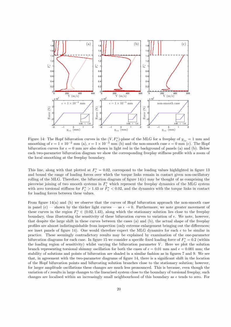
smoothing of ε = 1× 10−2 mm (a), ε = 1× 10−3 mm (b) and the non-smooth case ε = 0 mm (c). The Hopfbifurcation curves for ε = 0 mm are also shown in light red in the background of panels (a) and (b). Beloweach two-parameter bifurcation diagram we show the corresponding freeplay stiffness profile with a zoom ofthe local smoothing at the freeplay boundary.

This line, along with that plotted at F ∗z = 0.02, correspond to the loading values highlighted in figure 13

and bound the range of loading forces over which the torque links remain in contact given non-oscillatoryrolling of the MLG. Therefore, the bifurcation diagram of figure 14(c) may be thought of as comprising thepiecewise joining of two smooth systems in F ∗

z which represent the freeplay dynamics of the MLG systemwith zero torsional stiffness for F ∗

z > 1.43 or F ∗z < 0.02, and the dynamics with the torque links in contact

for loading forces between these values.

From figure 14(a) and (b) we observe that the curves of Hopf bifurcation approach the non-smooth casein panel (c) — shown by the thicker light curves — as ε → 0. Furthermore, we note greater movement ofthese curves in the region F ∗

z ∈ (0.02, 1.43), along which the stationary solution lies close to the freeplayboundary, thus illustrating the sensitivity of these bifurcation curves to variation of ε. We note, however,that despite the large shift in these curves between the cases (a) and (b), the actual shape of the freeplayprofiles are almost indistinguishable from inspection (only extreme enlargement bringing out the differences;see inset panels of figure 14). One would therefore expect the MLG dynamics for each ε to be similar inpractice. These seemingly contradictory results may be explained by examination of the one-parameterbifurcation diagrams for each case. In figure 15 we consider a specific fixed loading force of F ∗

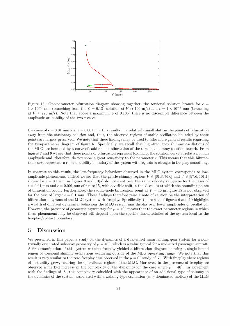
z = 0.2 (withinthe loading region of sensitivity) whilst varying the bifurcation parameter V . Here we plot the solutionbranch representing torsional shimmy oscillation for both the cases of ε = 0.01 mm and ε = 0.001 mm; thestability of solutions and points of bifurcation are shaded in a similar fashion as in figures 7 and 9. We seethat, in agreement with the two-parameter diagrams of figure 14, there is a significant shift in the locationof the Hopf bifurcation points and bifurcating solution branches close to the stationary solution; however,for larger amplitude oscillations these changes are much less pronounced. This is because, even though thevariation of ε results in large changes to the linearised system close to the boundary of torsional freeplay, suchchanges are localised within an increasingly small neighbourhood of this boundary as ε tends to zero. For

20

0 50 100 150 200 250

0.13

0.14

0.15

0.16

0.17

0.18

0.19

0.2

V (m/s)

Max

ψ(deg)

Figure 15: One-parameter bifurcation diagram showing together, the torsional solution branch for ε =1 × 10−2 mm (branching from the ψ = 0.13

solution at V ≈ 196 m/s) and ε = 1 × 10−3 mm (branching

at V ≈ 273 m/s). Note that above a maximum ψ of 0.135

there is no discernible difference between theamplitude or stability of the two ε cases.

the cases of ε = 0.01 mm and ε = 0.001 mm this results in a relatively small shift in the points of bifurcationaway from the stationary solution and, thus, the observed regions of stable oscillation bounded by thesepoints are largely preserved. We note that these findings may be used to infer more general results regardingthe two-parameter diagram of figure 6. Specifically, we recall that high-frequency shimmy oscillations ofthe MLG are bounded by a curve of saddle-node bifurcation of the torsional shimmy solution branch. Fromfigures 7 and 9 we see that these points of bifurcation represent folding of the solution curve at relatively highamplitude and, therefore, do not show a great sensitivity to the parameter ε. This means that this bifurca-tion curve represents a robust stability boundary of the system with regards to changes in freeplay smoothing.

In contrast to this result, the low-frequency behaviour observed in the MLG system corresponds to low-amplitude phenomena. Indeed we see that the gentle shimmy regions V ∈ [61.3, 76.6] and V ∈ [97.6, 101.1]shown for ε = 0.1 mm in figures 9 and 10(a) do not exist over the same velocity ranges as for the cases ofε = 0.01 mm and ε = 0.001 mm of figure 15, with a visible shift in the V -values at which the bounding pointsof bifurcation occur. Furthermore, the saddle-node bifurcation point at V = 40 in figure 15 is not observedfor the case of larger ε = 0.1 mm. These findings therefore raise a note of caution on the interpretation ofbifurcation diagrams of the MLG system with freeplay. Specifically, the results of figures 6 and 10 highlighta wealth of different dynamical behaviour the MLG system may display over lower amplitudes of oscillation.However, the presence of geometric asymmetry for µ = 40

means that the exact parameter regions in which

these phenomena may be observed will depend upon the specific characteristics of the system local to thefreeplay/contact boundary.

5 Discussion

We presented in this paper a study on the dynamics of a dual-wheel main landing gear system for a non-trivially orientated side-stay geometry of µ = 40

, which is a value typical for a mid-sized passenger aircraft.

A first examination of this system without freeplay yielded a bifurcation diagram showing a single boundregion of torsional shimmy oscillations occurring outside of the MLG operating range. We note that thisresult is very similar to the zero-freeplay case observed in the µ = 0

study of [7]. With freeplay these regions

of instability grew, entering the operational regime of the MLG. Moreover, in the presence of freeplay weobserved a marked increase in the complexity of the dynamics for the case where µ = 40

. In agreement

with the findings of [8], this complexity coincided with the appearance of an additional type of shimmy inthe dynamics of the system, associated with a walking-type oscillation (β, η dominated motion) of the MLG

21

system. This shimmy type was represented in the two-parameter results by the appearance of an additionalHopf bifurcation curve, from which branches of these oscillations bifurcate. We also observed new curves oftorus and period-doubling bifurcation, and together these features resulted in a wealth of different observabledynamics of the MLG system. In particular, the one-parameter bifurcation diagrams and simulation resultshighlighted the existence of multi-frequency periodic, quasi-periodic and chaotic-type oscillations. Further-more, these types of behaviour were found to coexist with higher amplitude torsional shimmy oscillations.We remark that such regions of multiple behaviour add a degree of uncertainty to the observed dynamics ofthe MLG in light of perturbing forces.

An additional point one may note is that a majority of these additional features were associated withrelatively small amplitude oscillation of the system. While these solutions may provide the seed of pertur-bation to higher amplitude phenomena, it is important to note that such small amplitude behaviour canalso be of direct significance from a physical perspective. Firstly, the results of the previous study [7] infer ascaling of these low amplitude phenomena with freeplay magnitude. One could therefore imagine a situationwhereby small scale oscillations of the MLG system could have a ‘loosening’ effect on the torque link assem-bly, gradually increasing the freeplay width; this in turn would produce larger oscillations still and thereforepresents a potential route to shimmy instability of greater severity. Although adequate maintenance checksof freeplay sources in the structure could alleviate such concerns, the accumulation of periodic instabilitycan still represent a source of structural fatigue. Secondly, the observed appearance of new shimmy modesand types of complex oscillation in this work introduce a range of additional frequencies into the system,any of which may potentially excite additional structural modes of the full aircraft + landing gear system.Possible adverse coupling can also arise via the interaction of these frequencies with the anti-skid and othercontrol systems. Whilst the detailed modelling of the entire aircraft structure, pertinent control systemsand longer-term ‘creep’ effects remains a challenge for future work, it is clear that the complex phenomenaobserved in this study, act to increase the susceptibility of the MLG system to shimmy instability.

We now consider the long and complex transient oscillation observed in the neighbourhood of weakly at-tracting solutions. When considering the variation of velocity V and loading force Fz during typical landingand take-off scenarios one realises that, in practice, the landing gear will not remain in the required (V, Fz)range for a sufficient length of time for these transients to settle down to the limiting behaviour. Therefore,despite the presence of attracting solutions, one would only expect to observe this transient motion. Simi-larly, we observed, both with and without freeplay, curves of Hopf bifurcation for very low Fz. These curvesappear within the operating region of the MLG and bound regions of low-amplitude shimmy oscillation.However, when considering the small range of light loading forces over which these oscillations exist, we notethat in practice, the MLG would pass very quickly through these regions, leaving insufficient time for suchoscillations to manifest themselves in the observed dynamics. Therefore, clearly a consideration of how theMLG system moves through the parameter space is important when interpreting these results.

A further consequence of the non-zero orientation µ = 40

was the introduction of geometric asymme-try into the system. This appeared in the dynamics as a lateral force perturbing the wheels from zero yaw.For the orientation studied, this resulted in a range of loading forces for which non-oscillatory behaviourrested close to the boundary of torsional freeplay. We found that, over this region, points of bifurcationfrom the stationary solution proved very sensitive to smoothing over the freeplay boundary. Specifically, weobserved large movement of the Hopf bifurcation curves of the system, even given very small changes in thesmoothing parameter ε. However, such small changes in ε yield very similar freeplay stiffness profiles and,in practice, one would expect the response of the system to remain largely the same for close ε values. Thisseemingly contradictory result was explained via examination of the bifurcation diagrams whereby we notedthat changes, although large, were localised about a small neighbourhood of the non-oscillatory solution;larger amplitude periodic solutions showed a greatly reduced sensitivity to the smoothing characteristicsover the freeplay region.

This observation prompted the introduction of the concept of robustness of stability boundaries. In par-

22

ticular, bifurcation curves comprising points of bifurcation along periodic solution branches of significantamplitude are robust with regards to localised changes to the freeplay region. This is a desirable propertyof the MLG model as factors such as the build-up of dirt, grease and corrosion mean that, in practice, onecannot be sure of the exact small-scale properties within the freeplay region of any real system; therefore,in the presence of this uncertainty these robust boundaries provide a greater degree of confidence in theparameter regions of instability.

Acknowledgements

The authors thank Duncan Pattrick and Phanikrishna Thota (Airbus in the UK) for useful discussions.This research was supported by a Knowledge Transfer Network (KTN) Mathematics CASE Award fromthe Engineering and Physical Sciences Research Council (EPSRC) in collaboration with Airbus in the UK.Simon Neild is supported by an EPSRC fellowship (EP/K005375/1).

References

[1] I. Besselink. Shimmy of aircraft main landing gears. PhD thesis, Delft University of Technology, 2000.

[2] F. Bohm and H. Willumeit. Dynamic behaviour of motorbikes. AGARD-R-800, 1996.

[3] R. Daugherty. A study of the mechanical properties of modern radial aircraft tires. Technical report,NASA/TM-2003-212415, Langley Research Center, Hampton, Virginia, 2003.

[4] M. Dengler, M. Goland, and G. Herrman. A bibliographic survey of automobile and aircraft wheelshimmy. Technical report, WADC 52-141, Midwest Research Institute, Kansas City, MO, USA, 1951.

[5] T. Gillespie. Fundamentals of vehicle dynamics. Society of Automotive Engineers, Inc., 1992.

[6] C. Howcroft. A bifurcation and numerical continuation study of aircraft main landing gear shimmy.PhD thesis, University of Bristol, 2013.

[7] C. Howcroft, B. Krauskopf, M. Lowenberg, and S. Neild. Effects of freeplay on dynamic stability of anaircraft main landing gear. Journal of Aircraft, 2013. doi: 10.2514/1.C032316.

[8] C. Howcroft, B. Krauskopf, M. Lowenberg, and S. Neild. Influence of variable side-stay geometry on theshimmy dynamics of an aircraft dual-wheel main landing gear. SIAM Journal on Applied DynamicalSystems, 12(3):1181–1209, 2013.

[9] P. Khapane. Simulation of landing gear dynamics using flexible multi-body methods. In 25th Interna-tional Congress of the Aeronautical Sciences, ISBN 0-9533991-7-6, 2006.

[10] R. Lernbeiss and M. Plochl. Simulation model of an aircraft landing gear considering elastic properties ofthe shock absorber. Proceedings of the Institute of Mechanical Engineers, Part K: Journal of Multi-bodyDynamics, 221:77–86, 2007.

[11] D. Limebeer, R. Sharp, and S. Evangelou. The stability of motorcycles under acceleration and braking.Proceedings of the Institute of Mechanical Engineers, Vol. 215, Part C, pages 1095–1109, 2001.

[12] Y-J. Lin and S-J. Hwang. Temperature prediction of rolling tires by computer simulation. Mathematicsand Computers in Simulation, 67(3):235–249, 2004.

[13] J. Mc Allen and A. Cuitino. Numerical investigation of the deformation characteristics and heat gener-ation in pneumatic aircraft tires: Part II. Thermal modeling. Finite Elements in Analysis and Design,23(2–4):265–290, 1996.

23

[14] H. Pacejka. Analysis of the shimmy phenomenon. Proceedings of the Institution of Mechanical Engineers:Automobile Division, 180(1):251–268, 1965.

[15] H. Pacejka. Mechanics of pneumatic tires, chapter Yaw and Camber Analysis, pages 757–839. US Dept.of Commerce, NBS Monograph Vol. 122, Washington, D.C., 1971.

[16] N. Plakhtienko and B. Shifrin. Critical shimmy speed of nonswiveling landing-gear wheels subject tolateral loading. International Applied Mechanics, 42(9):1077–1084, 2006.

[17] J. Pritchard. An overview of landing gear dynamics. Technical report, NASA/TM-1999-209143, 1999.

[18] B. Sateesh and D. Maiti. Non-linear analysis of a typical nose landing gear model with torsional freeplay.In Proc. IMechE Part G: J. Aerospace Engineering, volume 223(6), pages 627–641, 2009.

[19] S. Shaw and B. Balachandran. A review of nonlinear dynamics of mechanical systems in year 2008.Journal of System Design and Dynamics, 2(3):611–640, 2008.

[20] G. Somieski. Shimmy analysis of a simple aircraft nose landing gear model using different mathematicalmethods. Aerospace Science and Technology, 8:545–555, 1997.

[21] G. Stepan. Delay, nonlinear oscillations and shimmying wheels. In Application of nonlinear and chaoticdynamics in mechanics, volume 63 of Solid Mechanics and its Applications, pages 373–386. 1998.

[22] N. Sura and S. Suryanarayan. Lateral response of nonlinear nose-wheel landing gear models withtorsional free play. Journal of Aircraft, 44(6):1991–1997, 2007.

[23] D. Takacs and G. Stepan. Experiments on quasiperiodic wheel shimmy. Journal of Computational andNonlinear Dynamics, 4(3):031007, 2009.

[24] P. Thota, B. Krauskopf, and M. Lowenberg. Interaction of torsion and lateral bending in aircraft noselanding gear shimmy. Nonlinear Dynamics, 57(3):455–467, 2009.

[25] P. Thota, B. Krauskopf, and M. Lowenberg. Bifurcation analysis of nose landing gear shimmy withlateral and longitudinal bending. Journal of Aircraft, 47(1):87–95, 2010.

[26] R. Van der Valk and H. Pacejka. An analysis of a civil aircraft main gear shimmy failure. VehicleSystem Dynamics, 22(2):97–121, 1993.

[27] B. von Schlippe and R. Dietrich. Shimmying of a pneumatic wheel. Technical report, NACA TM 1365,1941.

[28] P. Woerner and O. Noel. Influence of nonlinearity on the shimmy behaviour of landing gear. AGARD-R-800, 1995.

24