Shifting and inhibition in cognitive control

Mario Gianni and Panagiotis Papadakis and Fiora PirriALCOR, Vision, Perception and Cognitive Robotics Laboratory

Department of Computer and System Sciences, University of Rome ‘La Sapienza‘, Italy{gianni, papadakis, pirri}@dis.uniroma1.it

Abstract— Shifting and inhibition are executive cognitivefunctions responding selectively to stimuli, so as to switchfrom one activity to a more compelling one or to inhibitinappropriate urges and preserve focus on the current task.In an autonomous system these cognitive skills are crucial toassess a well-regulated reactive behavior, which is of particularrelevance in critical circumstances. In this paper we develop anapproach to shifting and inhibition, as cost-response functions.These functions are defined within a rich probabilistic structuremodelling the stimuli and the way stimuli are taken into accountwhile the execution of a task. This is a preliminary account totask-switching in which we consider only the stimulus-responseside of the task switching, although to deem for the mainshifting and inhibition controls we have to introduce the conceptof tasks and related actions and constraints.

I. INTRODUCTION

Task switching is a crucial aspect of cognitive controlmodeling the human ability to adapt to changing circum-stances and stimuli. In fact, the ability to selectively respondto several stimuli, and to inhibit inappropriate urges, focusingon the task at hands, are well-known to exists in humansas shifting and inhibition executive functions [1], [2]).Theneuroscience theory of control uses inhibition to explainmany cognitive activities. First and foremost to explainhow a subject in the presence of several stimuli respondsselectively and is able to resist inappropriate urges (see[3]). Harnischfeger [4], [5] defines cognitive inhibition asa form of forgetting previously activated cognitive processesand harnessing interference from processes or contents notrelevant to the main current task. The executive functions ofinhibition and shifting explain the ability to flexibly switchbetween tasks, when a reconfiguration of memory is required,by disengaging from previous goals or task sets (see [6]). Ithas been observed that there is a switch cost that can beexplained by the previous task-set inhibition (see [7]).

Since the early work of Jersild [8] several studies in neuroand cognitive science have led to a better understanding ofmany of the variables affecting task switching in the contextof cognitive control (we refer the reader to [9]–[13] and thecitations therein).

These theories on executive control processes and taskswitching have strongly influenced cognitive robotics archi-tectures since the eighties, as for example the Norman andShallice [14] ATA schema and the principles of goal directedbehaviors in Newell [15] (for a review on these architecturesin the framework of the task switching paradigm see [16]).

However only recently the need to model task switchingand the cognitive functions of shifting and inhibition, under-

lying the cognitive control ability to switch, are becominga hot topic in cognitive robotics. Earliest studies have beencarried within brain-actuated interaction [17], mechatronic[18], learning [19] and planning [20]. Recently severalstudies have posed the need to model task switching tocope with adaptivity and ecological behaviors in a dynamicenvironment, such as [21]–[26].

Experts of task switching claim that the decision under-goes a switching cost. This cost results from the interplaybetween the time needed to reconfigure a mental state andthe time needed to resolve interference from a previous set[12].

In this paper we describe an approach to shifting andinhibition, based on the concept of a switching cost toreconfigure a mental state and the time needed to resolveinterference from a previous set [12] by modeling the re-configuration of a new task given the incoming stimuli andthe current state. The approach models how to compute thestimuli, the stimuli cost, measured according to the currenttask and, finally, the response. This preliminary model isembedded into a planning framework [27], [28] that we donot discuss here.

We consider stimuli occurring in time, and by attributinga cost to them we can decide whether the current actionsis to be interrupt if the stimuli is afforded, or if it shouldcontinue and the stimuli disregarded.

The paper is organized as follows. In the next Section IIwe introduce some preliminary concepts of the framework; inSection III, we introduce the measures to evaluate the stimulicost. Further we illustrate the response model in Section IVand in Section V we illustrate the method for choosing theminimal cost response, if this exists. The paper is concludedwith some indication on possible future directions.

II. PRELIMINARY DEFINITIONS

In this section we introduce some preliminary definitionsconcerning processes, the state of the system, the timelinesfor assessing both reaction times (RT) and the responsestimulus intervals, and the specification of a task. As reportedin the literature, task switching incurs into a switching cost.Monsell and colleagues [29] have studied what counts toreduce this cost, according to preparation – to the stimulusonset – and demonstrated that reaction time depends on thepreparation to task changes, namely mean RT is longer (anderror rate usually greater) when the task changes than whenthe same task is performed as on the previous trial. Still thereis a residual cost [30] [29]. This unavoidable cost is crucial to

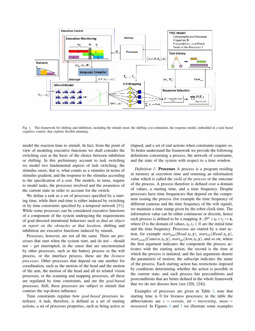
Fig. 1. The framework for shifting and inhibition, including the stimuli onset, the shifting cost estimation, the response model, embedded in a task basedcognitive control, that exploits flexible planning.

model the reaction time to stimuli. In fact, from the point ofview of modeling executive functions we shall consider theswitching cost at the basis of the choice between inhibitionor shifting. In this preliminary account to task switchingwe model two fundamental aspects of task switching, thestimulus onset, that is, what counts as a stimulus in terms ofstimulus gradient, and the response to the stimulus accordingto the specification of a cost. The models, in turns, requireto model tasks, the processes involved and the awareness ofthe current state in order to account for the switch.

We define a task as a set of processes specified by a start-ing time, while their end-time is either induced by switchingor by time constraints specified by a temporal network [31].While some processes can be considered executive functionsof a component of the system undergoing the requirementsof goal-directed intentional behaviors such as find an objector report on the obstacles at that location, shifting andinhibition are executive functions induced by stimuli.

Processes, however, are not all the same. There are pro-cesses that start when the system start, and do not – shouldnot – get interrupted, in the sense that are unconstrainedby other processes, such as the battery process or the wifiprocess, or the interface process, these are the livenessprocesses. Other processes that depend on one another forcoordination, such as the motion of the head and the motionof the arm, the motion of the head and all its related visionprocesses, or the scanning and mapping processes, all theseare regulated by time constraints, and are the goal-basedprocesses. Still, these processes are subject to stimuli thatcontrast the top-down influence.

Time constraints regulate how goal-based processes in-terleave. A task, therefore, is defined as a set of startingactions, a set of processes properties, such as being active or

elapsed, and a set of end actions when constraints require so.To better understand the framework we provide the followingdefinitions concerning a process, the network of constraints,and the state of the system with respect to a time window.

Definition 1: Processes A process is a program residingin memory at execution time and returning an informationvalue which is called the yield of the process or the outcomeof the process. A process therefore is defined over a domainof values, a starting time, and a time frequency. Despiteprocesses have time frequencies that depend on the compo-nent issuing the process (for example the time frequency ofdifferent cameras and the time frequency of the wifi signal),we maintain a time stamp given by the robot clock time. Theinformation value can be either continuous or discrete, henceeach process is defined to be a mapping π : Dm× t0× t f 7→ x,where D is the domain of values, t0, t f ∈R are the initial timeand the time frequency. Processes are started by a start ac-tion, for example startpan(Head, t0,y), starttilt(Head, t0,y),startzoom(Camera, t0,y), startup(Arm, t0,y), and so on, wherethe first argument indicates the component the process ac-tivates with the starting action, the second is the time atwhich the process is initiated, and the last arguments denotethe parameters of motion; the subscript indicates the nameof the process. Each starting action has restrictions imposedby conditions determining whether the action is possible inthe current state, and each process has preconditions andpostconditions that are better defined in the whole frameworkthat we do not discuss here (see [20], [24]).

Examples of processes are given in Table I, note thatstarting time is 0 for liveness processes; in the table theabbreviations are c = certain, int = interesting, meas =measured. In Figures 4 and 5 we illustrate some examples

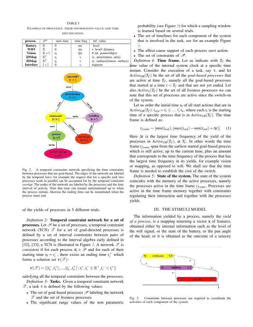
TABLE IEXAMPLE OF PROCESSES, THEIR INFORMATION VALUE AND TIME

SPECIFICATION.

process. Dm start time time freq inf. valueBattery R 0 ms levelWIFI R 0 ms s. level/ distanceVision R× I t0 fps # int. points/object

2DMap R2 tk s (c. area)/(meas. area)3DMap R2 tk s (c. surface)/(meas. surface)

Interface I× I 0 s requests

Fig. 2. A temporal constraints network specifying the time constraintsbetween processes that are goal-based. The edges of the network are labeledby the temporal laws; for example the request that for a specific task twoprocesses work in parallel can be accounted for by the temporal constraintoverlap. The nodes of the network are labeled by the processes and the timeinterval of activity. Note that time can remain uninstantiated up to whenthe process initiate, likewise the ending time can be instantiated when theprocess must end.

of the yields of processes in 5 different trials.

Definition 2: Temporal constraint network for a set ofprocesses. Let P be a set of processes, a temporal constraintnetwork (TCN) T for a set of goal-directed processes isdefined by a set of interval constraints between pairs ofprocesses according to the interval algebra early defined in[32], [33]; a TCN is illustrated in Figure 2. A network T isconsistent if for each process πi ∈P and for each of theirstarting time t0 = t−i , there exists an ending time t+i whichforms a solution set ν(T ):

ν(T ) = {[t−1 , t+1 ], ..., [t−n , t+n ] : t+i , t−i ∈ R+, t−i < t+i }

satisfying all the temporal constraints between the processes.Definition 3: Tasks. Given a temporal constraint network

T , a task τ is defined by the following values:• The set of goal-based processes P labeling the network

T and the set of liveness processes.• The significant range values of the non parametric

probability (see Figure 5) for which a sampling windowis learned based on several trials.

• The set of timelines for each component of the systemthat is involved in the task, see for an example Figure3.

• The effect-cause support of each process start action.• The set of constraints of P .Definition 4: Time frame. Let us indicate with TC the

time value of the internal system clock at a specific timeinstant. Consider the execution of a task, say τ , and letActiveGB(TC) be the set of all the goal-based processes thatare active at time TC, namely all the goal-based processesthat started at a time t < TC and that are not yet ended. Letalso ActiveL(TC) be the set of all liveness processes we cannote that this set of processes are active since the switch-onof the system.

Let us order the initial time t0 of all start actions that are inActiveGB(TC): tord = t1≤ . . .≤ tn, where each ti is the startingtime of a specific process that is in ActiveGB(TC). The timeframe is defined as:

t f rame = [min(tord),(max(tord)−min(tord)+∆t)] (1)

Here ∆t is the largest time frequency of the yield of theprocesses in ActiveGB(TC), at TC. In other words the timeframe t f rame span from the earliest started goal-based processwhich is still active, up to the current time, plus an amountthat corresponds to the time frequency of the process that hasthe largest time frequency in its yields, for example visionor mapping, as opposed to wifi. We shall see that the timeframe is needed to establish the cost of the switch.

Definition 5: State of the system. The state of the systemcoincides with the memory of the active processes, namelythe processes active in the time frame t f rame. Processes areactive in the time frame memory together with constraintsregulating their interaction and together with the processesyields.

III. THE STIMULI MODEL

The information yielded by a process, namely the yieldof a process, is a mapping returning a vector x of features,obtained either by internal information such as the level ofthe wifi signal, or the state of the battery, or the pan angleof the head; or it is obtained as the outcome of a sensory

Fig. 3. Constraints between processes are required to coordinate theactivities of each component of the system.

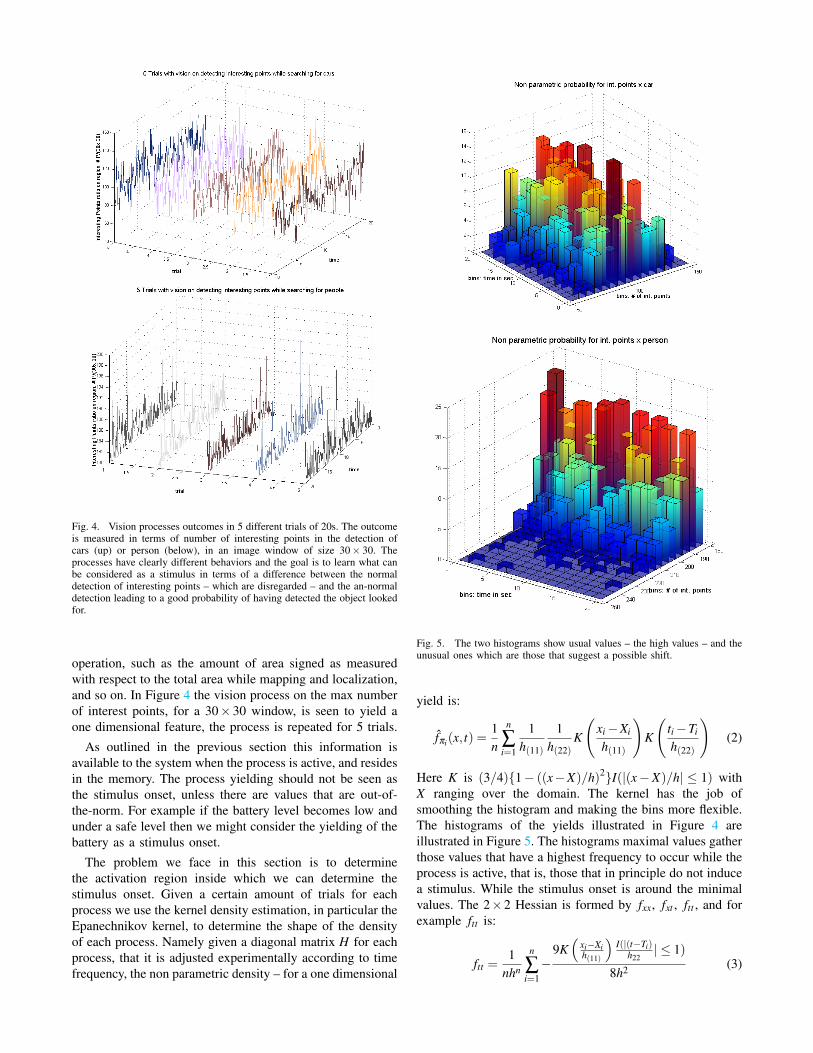
Fig. 4. Vision processes outcomes in 5 different trials of 20s. The outcomeis measured in terms of number of interesting points in the detection ofcars (up) or person (below), in an image window of size 30× 30. Theprocesses have clearly different behaviors and the goal is to learn what canbe considered as a stimulus in terms of a difference between the normaldetection of interesting points – which are disregarded – and the an-normaldetection leading to a good probability of having detected the object lookedfor.

operation, such as the amount of area signed as measuredwith respect to the total area while mapping and localization,and so on. In Figure 4 the vision process on the max numberof interest points, for a 30× 30 window, is seen to yield aone dimensional feature, the process is repeated for 5 trials.

As outlined in the previous section this information isavailable to the system when the process is active, and residesin the memory. The process yielding should not be seen asthe stimulus onset, unless there are values that are out-of-the-norm. For example if the battery level becomes low andunder a safe level then we might consider the yielding of thebattery as a stimulus onset.

The problem we face in this section is to determinethe activation region inside which we can determine thestimulus onset. Given a certain amount of trials for eachprocess we use the kernel density estimation, in particular theEpanechnikov kernel, to determine the shape of the densityof each process. Namely given a diagonal matrix H for eachprocess, that it is adjusted experimentally according to timefrequency, the non parametric density – for a one dimensional

Fig. 5. The two histograms show usual values – the high values – and theunusual ones which are those that suggest a possible shift.

yield is:

fπi(x, t) =1n

n

∑i=1

1h(11)

1h(22)

K

(xi−Xi

h(11)

)K

(ti−Ti

h(22)

)(2)

Here K is (3/4){1− ((x−X)/h)2}I(|(x−X)/h| ≤ 1) withX ranging over the domain. The kernel has the job ofsmoothing the histogram and making the bins more flexible.The histograms of the yields illustrated in Figure 4 areillustrated in Figure 5. The histograms maximal values gatherthose values that have a highest frequency to occur while theprocess is active, that is, those that in principle do not inducea stimulus. While the stimulus onset is around the minimalvalues. The 2×2 Hessian is formed by fxx, fxt , ftt , and forexample ftt is:

ftt =1

nhn

n

∑i=1−

9K(

xi−Xih(11)

)I(|(t−Ti)

h22| ≤ 1)

8h2 (3)

-3 -2 -1 0 1 2 3

0.0

0.2

0.4

0.6

0.8

1.0

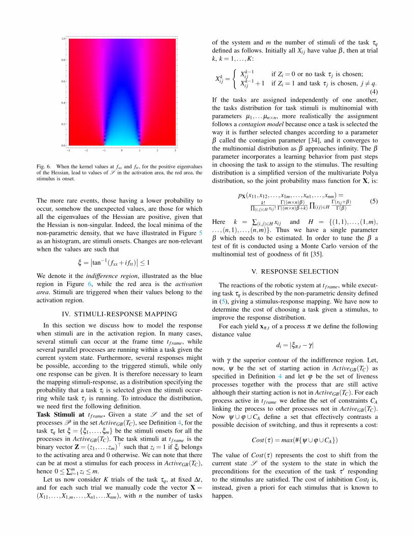
Fig. 6. When the kernel values at fxx and ftt , for the positive eigenvaluesof the Hessian, lead to values of S in the activation area, the red area, thestimulus is onset.

The more rare events, those having a lower probability tooccur, somehow the unexpected values, are those for whichall the eigenvalues of the Hessian are positive, given thatthe Hessian is non-singular. Indeed, the local minima of thenon-parametric density, that we have illustrated in Figure 5as an histogram, are stimuli onsets. Changes are non-relevantwhen the values are such that

ξ =∣∣tan−1( fxx + i ftt)

∣∣≤ 1

We denote it the indifference region, illustrated as the blueregion in Figure 6, while the red area is the activationarea. Stimuli are triggered when their values belong to theactivation region.

IV. STIMULI-RESPONSE MAPPING

In this section we discuss how to model the responsewhen stimuli are in the activation region. In many cases,several stimuli can occur at the frame time t f rame, whileseveral parallel processes are running within a task given thecurrent system state. Furthermore, several responses mightbe possible, according to the triggered stimuli, while onlyone response can be given. It is therefore necessary to learnthe mapping stimuli-response, as a distribution specifying theprobability that a task τi is selected given the stimuli occur-ring while task τ j is running. To introduce the distribution,we need first the following definition.Task Stimuli at t f rame. Given a state S and the set ofprocesses P in the set ActiveGB(TC), see Definition 4, for thetask τq let ξ = {ξ1, . . . ,ξm} be the stimuli onsets for all theprocesses in ActiveGB(TC). The task stimuli at t f rame is thebinary vector Z = (z1, . . . ,zm)

> such that zi = 1 if ξi belongsto the activating area and 0 otherwise. We can note that therecan be at most a stimulus for each process in ActiveGB(TC),hence 0≤ ∑

mi=1 zi ≤ m.

Let us now consider K trials of the task τq, at fixed ∆t,and for each such trial we manually code the vector X =(X11, . . . ,X1,m, . . . ,Xn1, . . .Xnm), with n the number of tasks

of the system and m the number of stimuli of the task τqdefined as follows. Initially all Xi j have value β , then at trialk, k = 1, . . . ,K:

Xki j =

{Xk−1

i j if Zi = 0 or no task τ j is chosen;Xk−1

i j +1 if Zi = 1 and task τ j is chosen, j 6= q.(4)

If the tasks are assigned independently of one another,the tasks distribution for task stimuli is multinomial withparameters µ1, . . .µn×n, more realistically the assignmentfollows a contagion model because once a task is selected theway it is further selected changes according to a parameterβ called the contagion parameter [34], and it converges tothe multinomial distribution as β approaches infinity. The β

parameter incorporates a learning behavior from past stepsin choosing the task to assign to the stimulus. The resultingdistribution is a simplified version of the multivariate Polyadistribution, so the joint probability mass function for X, is:

pX(x11,x12, . . . ,x1m, . . . ,xn1, . . . ,xnm) =k!

∏(i, j)∈H xi j!Γ((m×n)β )

Γ((m×n)β+k) ∏(i j)∈HΓ(xi j+β )

Γ(β )

(5)

Here k = ∑(i, j)∈H xi j and H = {(1,1), . . . ,(1,m),. . . ,(n,1), . . . ,(n,m)}. Thus we have a single parameterβ which needs to be estimated. In order to tune the β atest of fit is conducted using a Monte Carlo version of themultinomial test of goodness of fit [35].

V. RESPONSE SELECTION

The reactions of the robotic system at t f rame, while execut-ing task τq is described by the non-parametric density definedin (5), giving a stimulus-response mapping. We have now todetermine the cost of choosing a task given a stimulus, toimprove the response distribution.

For each yield xπ,t of a process π we define the followingdistance value

di = |ξπ,t − γ|

with γ the superior contour of the indifference region. Let,now, ψ be the set of starting action in ActiveGB(TC) asspecified in Definition 4 and let ϕ be the set of livenessprocesses together with the process that are still activealthough their starting action is not in ActiveGB(TC). For eachprocess active in t f rame we define the set of constraints CAlinking the process to other processes not in ActiveGB(TC).Now ψ ∪ ϕ ∪CA define a set that effectively contrasts apossible decision of switching, and thus it represents a cost:

Cost(τ) = max(#{ψ ∪ϕ ∪CA})

The value of Cost(τ) represents the cost to shift from thecurrent state S of the system to the state in which thepreconditions for the execution of the task τ ′ respondingto the stimulus are satisfied. The cost of inhibition CostI is,instead, given a priori for each stimulus that is known tohappen.

Given the specifications Ξ = {τ1, . . . ,τn} (see 3) of thesystem, we define a function F : Ξ→R as follows

F(τ) = w

(K

∑k=1

dkδk

)f (ψ) (6)

here w is the weight of the task and δk ∈ {0,1} selects whichdistances dk further weights the task according to the stimuli-response mapping.

The reaction to the stimuli occurrence is selected bysolving the following optimization problem

minimizeτi∈Ξ

F(τi)

subject to Cost(τ)≤CostI(ξ )i, i = 1, . . . ,n.

If no solution τi of the problem exists, then the stimuli isinhibited.

VI. CONCLUSION

In this paper we have introduced a preliminary model fortask switching facing the stimuli onset, the switch cost andfinally the response model. The topic is becoming of greatinterest in the cognitive robotics community, likewise in theattention and vision communities, as it faces an importantproblem: modeling processes as means for inducing changesin goal-based behaviors so as to ensure adaptation to achanging environment. Clearly, we face different scenarios,from those devised by neuroscience, and thus our paradigmsare slightly different. Still, the main difficulty concerns all theimplications of shifting and inhibition, in terms of responsetime and intervals as studied in deep details in neuroscience;on the other hand there is the need of the modeling thecomplete framework on which task-switching can be based,since the definition of the cost requires a clear understandingof all the connections of a process with other ones, like futureprocesses, linked to the present ones, by constraints. This are,indeed, the aims of the ongoing research.

REFERENCES

[1] E. Miller and J. Cohen, “An integrative theory of prefrontal cortexfunction,” Annual Rev. Neuroscience, vol. 24, pp. 167 – 202, 2007. 1

[2] A. R. Aron, “The neural basis of inhibition in cognitive control,” TheNeuroscientist, vol. 13, pp. 214 – 228, 2007. 1

[3] S. P. Tipper, “Does negative priming reflect inhibitory mechanisms?a review and integration of conflicting views,” Quarterly Journal ofExperimental Psychology, vol. 54, pp. 321 – 343, 2001. 1

[4] K. K. Harnishfeger and D. F. Bjorklund, The evolution of inhibitionmechanisms and their role in human cognition and behavior., 1995,pp. 141 – 173. 1

[5] K. Kipp and R. S. Pope, “Intending to forget: The development ofcognitive inhibition in directed forgetting,” Journal of ExperimentalChild Psychology, vol. 62, pp. 292 – 315, 1996. 1

[6] U. Mayr and S. Keele, “Changing internal constraints on action: therole of backward inhibition.” Journal of Experimental Psychology, vol.129, no. 1, pp. 4–26, 2000. 1

[7] A. Philipp and I. Koch, “Task inhibition and task repetition in taskswitching,” The European Journal of Cognitive Psychology, vol. 18,no. 4, pp. 624–639, 2006. 1

[8] A. Jersild, “Mental set and shift.” Archives of Psychology, vol. 89, pp.5–82, 1927. 1

[9] R. Rogers and S. Monsell, “The costs of a predictable switch betweensimple cognitive tasks,” J. of Exp. Psychology: General, vol. 124, pp.207–231, 1995. 1

[10] Thea and Ionescu, “Exploring the nature of cognitive flexibility,” NewIdeas in Psych., vol. 30, no. 2, pp. 190 – 200, 2012. 1

[11] C. Chamberland and S. Tremblay, “Task switching and serial memory:Looking into the nature of switches and tasks,” Acta Psych., vol. 136,pp. 137–147, 2011. 1

[12] S. Monsell, “Task switching,” Trends in Cognitive Sciences, vol. 7,no. 3, pp. 134 – 140, 2003. 1

[13] J. Rubinstein, D. Meyer, and E.Jeffrey, “Executive control of cognitiveprocesses in task switching.” J. of Exp. Psych.: Human Perception andPerformance, vol. 27, no. 4, pp. 763–797, 2001. 1

[14] D. A. Norman and T. Shallice, Consciousness and Self-Regulation:Advances in Research and Theory. Plenum Press, 1986, vol. 4, ch.Attention to action: Willed and automatic control of behaviour. 1

[15] A. Newell, Unified theories of cognition. Harvard University Press,1990. 1

[16] J. Rubinstein, E. Meyer, and J. E. Evans, “Executive control of cogni-tive processes in task switching,” Journal of Experimental Psychology:Human Perception and Performance, vol. 27, no. 4, pp. 763–797, 2001.1

[17] J. d. R. Milln, F. Renkens, J. Mourio, and W. Gerstner, “Brain-actuatedinteraction,” Artificial Intelligence, vol. 159, pp. 241–259, 2004. 1

[18] G. Capi, “Robot task switching in complex environments,” in Ad-vanced intelligent mechatronics, 2007 IEEE/ASME international con-ference on, 2007, pp. 1 –6. 1

[19] M. Ito, K. Noda, Y. Hoshino, and J. Tani, “Dynamic and interactivegeneration of object handling behaviors by a small humanoid robotusing a dynamic neural network model,” Neural Networks, vol. 19,pp. 323–337, 2006. 1

[20] A. Finzi and F. Pirri, “Representing flexible temporal behaviors in thesituation calculus,” in In Proc. of IJCAI, 2005. 1, 3

[21] G. Capi, G. Pojani, and S.-I. Kaneko, “Evolution of task switchingbehaviors in real mobile robots,” in Innovative Computing Informationand Control, 2008. ICICIC ’08. 3rd International Conference on, 2008,p. 495. 1

[22] S. Suzuki, T. Sasaki, and F. Harashima, “Visible classification oftask-switching strategies in vehicle operation,” in Robot and HumanInteractive Communication, 2009. RO-MAN 2009. The 18th IEEEInternational Symposium on, 2009, pp. 1161 –1166. 1

[23] J. Wawerla and R. Vaughan, “Robot task switching under diminish-ing returns,” in Intelligent Robots and Systems, 2009. IROS 2009.IEEE/RSJ International Conference on, 2009, pp. 5033 –5038. 1

[24] A. Finzi and F. Pirri, “Switching tasks and flexible reasoning in thesituation calculus,” DIS Sapienza Universita di Roma, Tech. Rep. 7,2010. 1, 3

[25] K. Durkee, C. Shabarekh, C. Jackson, and G. Ganberg, “Flexibleautonomous support to aid context and task switching,” in CognitiveMethods in Situation Awareness and Decision Support (CogSIMA),2011 IEEE First International Multi-Disciplinary Conference on,2011, pp. 204 –207. 1

[26] D. D’Ambrosio, J. Lehman, S. Risi, and K. Stanley, “Task switchingin multirobot learning through indirect encoding,” in Intelligent Robotsand Systems (IROS), 2011 IEEE/RSJ International Conference on,2011, pp. 2802 –2809. 1

[27] A. Finzi, F. Pirri, Ray, and R. Reiter, “Open world planning in thesituation calculus,” in In Proc. of (AAAI-2000). AAAI Press, 1999,pp. 754–760. 1

[28] F. Pirri and R. Reiter, “Some contributions to the metatheory of thesituation calculus,” J. ACM, vol. 46, no. 3, pp. 325–361, 1999. 1

[29] S. Nieuwenhuis and S. Monsell, “Residual cost in task switching:Testing the failure to engage hypothesis,” Psychonomic Bulletin andReview, vol. 1, no. 9, pp. 86 – 92, 2002. 1

[30] R. Rogers and S. Monsell, “osts of a predictable switch between simplecognitive tasks,” Journal of Experimental Psychology: General, no.124, pp. 207 – 231, 1995. 1

[31] I. Meiri, “Combining qualitative and quantitative constraints in tem-poral reasoning,” J. Art. Intel., pp. 260–267, 1996. 2

[32] R. Dechter, I. Meiri, and J. Pearl, “Temporal constraint networks,”Artif. Intell., vol. 49, no. 1-3, pp. 61–95, 1991. 3

[33] M. Vilain, H. Kautz, and P. Beek, “Constraint propagation algorithmsfor temporal reasoning,” in Readings in Qualitative Reasoning aboutPhysical Systems. Morgan Kaufmann, 1986, pp. 377–382. 3

[34] P. Kvam and D. Day, “The multivariate polya distribution in combatmodeling,” Naval Res. Logistics, vol. 48, no. 1, pp. 1–17, 2001. 5

[35] J. R. Taylor, An introduction to error analysis. USB, 1997. 5