Shielding Store Brands: A Large–Scale Field Experiment

Eric T. Anderson

Kellogg School of Management

Northwestern University

eric-anderson@kellogg.northwestern.edu

Karsten T. Hansen

Rady School of Management

UC San Diego

k4hansen@ucsd.edu

Duncan Simester

Sloan School of Management

MIT

simester@mit.edu

June 15, 2012

1

Abstract

In this paper, we report on the results of a large-scale field experiment that was

designed to investigate whether store brands should be discounted when a national brand

is promoted (a retail practice called “shielding”). Our experiment focuses on 28 “copycat”

store brands and the corresponding national brand that are sold in a large number of stores

of a national retailer. On weeks where the national brand is promoted we experimentally

vary the price level of the copycat store brand. The experimental design includes a

control with no store brand discount and five additional conditions in which the store

brand was discounted by as much as 40%. Since prices are randomized among only six

geographic regions, we develop an econometric model that integrates historical data and

experimental data in a unified framework. This allows us to recover treatment effects and

investigate how to optimally shield store brands against national brand price promotions.

We find that shielding the store brand from national brand promotions leads to both a

substitution effect and a category expansion effect. While the category expansion effect

on average dominates the substitution effect, we find heterogeneity in the size of the

two effects across categories. Our findings indicate that – in general – it is preferable to

engage in shielding. Across the 28 categories in the sample, the average optimal shielding

level is a 17 percent discount off the regular price. This leads to an average increase in

category profit of 21.6 percent compared to a strategy of no shielding. We also investigate

the extent to which simple managerial shielding heuristics can mimic optimal shielding

levels. We find that following a simple “price gap maintenance” heuristic, a manager can

on average increase profits by 7.9 percent compared to a strategy of no shielding. This

is a little more than a third of the profit increase achieved from an optimal shielding

strategy.

Key words: Store Brands, Pricing, Retail, Field Experiment.

2

1 Introduction

National brands spent over $176 billion in 2010 to promote their brands in retail stores. A

large part of these dollars are directed at reducing the national brand price. Recently there

has been an active debate in the marketing literature about whether or not retailers react

to these trade promotions by lowering the prices of competing products (Besanko, Dube and

Gupta (2005), McAlister (2007), Dube and Gupta (2005)). A simple category pricing model

suggests that this should occur: if a promotion on one item affects demand for other items it

will generally be profitable to change the prices of all affected items. This is particularly true

when the promoted item is a national brand and the affected item is a store brand/private

label brand for which the retailer enjoys a larger profit margin.1 If the price of the store

brand is left unchanged, the promotion on the national brand may cannibalize sales from the

store brand and lower overall profits. To avoid this, some retailers engage in a practice called

shielding. This amounts to lowering the price of the store brand during weeks of national

brand promotions. This will potentially mitigate the negative impact of the national brand’s

lower price.

In this paper, we report on the results of a large-scale field experiment that was designed

to investigate how store brands should be priced when a national brand is promoted. Our

experiment focuses on 28 “copycat” store brands and the corresponding national brand (see

Kumar and Steenkamp (2007)) that are sold in a very large number of stores of a national

retailer. On weeks where the national brand is promoted we experimentally vary the price

level of the copycat store brand. The experimental design includes a control with no store

brand discount and five additional conditions in which the store brand was discounted by

as much as 40%. This allows us to investigate how to optimally price the store brand (i.e.,

“shield” the store brand) during national brand price promotion weeks.

We show that the shielding decision is an important managerial decision from an economic

perspective, since a large amount of category volume and revenue is generated during promo-

tion weeks. Furthermore, we show that identifying shielding effects from historical sales and

price data for a category is quite hard: In our data we observe between one to seven national

brand promotion events per category over a 30 week time period. Since shielding effects

are defined during promotion weeks, this leaves us with very little data. In addition, both

national brand price and the store brand price often move together during promotion weeks,

making the identification of store brand price promotions even harder. We show that due to

the data limitations in historical data, a standard demand model provides fairly unrealistic

effects of shielding for many categories. This leads us to use a field experiment to identify

shielding effects.

Our analysis proceeds in several steps that integrate historical data and experimental data

1In the following we use “store brand” and “private label brand” interchangeably.

3

in a unified framework. Importantly, we illustrate the value of combining historical data with

experimental data. We demonstrate this through three phases of analysis. In the first phase,

we estimate a standard demand model that utilizes only historical data (pre-experiment). We

show that there is limited direct information in the historical data about shielding effects,

and as a result, the predictions from the demand model are based on extrapolations that fall

outside the historical variation in the data. Relying on these extrapolations for managerial

decision making requires a lot of faith in the structure of the estimated demand model.

Next, we move to a model that utilizes only the experimental data and ignores historical

data. This essentially amounts to a simple comparison of means across treatment conditions,

which avoids the pitfalls of a misspecified demand model (by not relying on a model at

all). However, while we have a large number of stores in the experiment, the retailer’s

systems do not allow random variation of prices across each individual store. Instead, the

unit of randomization is an individual region, and so while all stores in the same geographic

region have the same prices, these prices vary across the retailer’s six geographic regions.

This reflects a common challenge when conducting experiments in the field. Organizational

obstacles often require experimental variation at a more aggregate level than we might wish.

Because there are only six regions, randomization is not sufficient to control for any differences

between the regions. Instead, we use transaction data from the weeks prior to the experiments

to econometrically control for region differences. This approach effectively combines the

historical data with the experimental data. The historical data can be used as an implicit

control for pre-treatment unobserved heterogeneity, and we show that this analysis leads to

treatment effects estimates that are much more reasonable. to the Introduction.

Our empirical findings are as follows. We find large effects of shielding on store brand

sales. When converted to elasticities, the estimated shielding effects imply elasticities between

-2 to -4 for most categories. For about two thirds of the 28 categories, we find fairly small

effects of shielding on national brand sales. For these categories the practice of shielding does

not lead to substitution away from the national brand, but rather to an expansion of the

category. For the remaining one third of categories, the expansion of the category is minor

and the substitution towards the store brand in stronger. However, on average the category

expansion effect dominates: Across the 28 categories, total category unit sales is about 25

percent bigger at the highest shielding level compared to no shielding.

Using the estimated shielding effects, we compute optimal shielding levels by predicting

profit at different shielding levels. For most categories we find that moderate amounts of

shielding is optimal. The average optimal shielding level is a 17 percent discount off the

regular store brand price. However, for some categories no shielding is optimal, while for

others shielding above 30 percent is recommended. Our results imply that following a strategy

of optimal shielding increases profit by an average of 21.6 percent compared to a strategy

of no shielding. For some categories the incremental gain in profit is above 80 percent. We

4

explore which category factors are predictive of the optimal shielding level. We find that the

store brand elasticity is highly correlated with optimal shielding levels.

We also evaluate two managerial shielding heuristics. These are based on matching the

discount of the national brand – either in percentage terms (percent gap maintenance) or

in absolute dollar terms (dollar gap maintenance). We find that following a dollar gap

maintenance strategy results in a 7.9 percent increase in profit compared to no shielding, while

a percent gap heuristic increases profit by 6.1 percent on average. This is to be compared to

the 21.6 percent increase in profit from following the optimal shielding strategy.

We start the paper with a literature review in Section 2. Section 3 provides a definition of

shielding effects, while Section 4 discusses the identification of shielding effects from historical

data. In Section 5 we present the field experiment used for the main results in the paper.

Section 6 outlines the econometric strategy underlying our empirical results. In Section 7 we

present and discuss the main findings, while Section 8 contains results for optimal shielding

and evaluation of managerial heuristics. Section 9 concludes.

2 Literature Review

Our findings contribute to the literatures on private label brands and category management.

2.1 Category Pricing

Category management is a complex process that is of considerable importance to retailers.

One key to successful retail category management is correctly pricing multiple brands within

a category. This task is analogous to the manufacturer problem of pricing a product line (e.g.,

Zenor (1994)). There is an extensive theoretical literature on category pricing. We focus on

situations where a retailer sells a portfolio of substitute products (Mussa and Rosen (1978)).

If products have positive cross-price elasticities, then price changes on one item necessitate

contemporaneous price changes on competing items (see for example Simester (1997) Lee and

Staelin (1997), Shugan and Desiraju (2001) and Moorthy (2005). Recent empirical research

estimate these cross-price elasticities and illustrate the category pricing problem. Examples

include Besanko, Gupta and Jain (1998), Villas-Boas and Zhao (2005), Meza and Sudhir

(2006) and Villas-Boas (2007).

A debate recently surfaced about whether cross-brand pass-through exists in practice.

Besanko, Dube and Gupta (2005) use a sample of the Dominick’s Finer Foods database and

find significant evidence that cross-brand pass-through exists and depends upon the relative

size and shares of the brands. These findings were later criticized by McAlister (2007), who

argued that the analysis did not account for the inter-dependence of prices across pricing

zones. In a follow-up paper, Dube and Gupta (2005) respond to this criticism by reanalyzing

5

their data using a different methodology, and supplementing it with a longer series of more

aggregate data. Their findings confirm the original Besanko, Dube and Gupta (2005) results,

although the magnitude of the effects are smaller. In our paper the focus shifts from whether

retailers engage in cross-brand pass-through of trade promotions to an evaluation of the

profitability of pass-through strategies.

2.2 Private Label/Store Brand

Over the last thirty years, private label or store brands have steadily grown and now represent

a substantial fraction of sales. In 2009, private label share in the UK was 43% while in

the more fragmented U.S. retail market private label garnered 17% share2. Tesco touts its

Finest brand as the largest food brand in the UK while Walmart’s Great Value brand is

the largest global brand. Private label brands have extended beyond lower quality/lower

priced alternatives that were originally introduced in the late 1970’s. Today, private label

brands can be categorized into three broad groups: national brand copycats (e.g. Walgreen’s

Wal-dryl and Benedryl), premium private label (Target’s Archer Farms) and value innovators

like Ikea (Kumar and Steenkamp (2007)). As private label brands have grown in importance

retailers have added organizational capabilities. Leading retailers like Walmart, Target and

Office Max have recently created private label brand management groups. The result of these

changes is that private label brands have grown in both importance and scope.

Recent academic research has sought to understand why consumers are willing to pay

a premium for national brands vs. store brand alternatives. Steenkamp, Van Heerde and

Geyskens (2010) find that if store brands are in the early stages of growth then advertising

and package design can influence the premium that customers will pay for a national brand.

However, as private labels mature, manufacturing and innovation become relatively more

important. This builds on earlier findings by Sethuraman and Cole (1999), who show that

12% of the national brand vs. private label price gap is explained by quality perceptions.

Similarly, Hoch and Lodish (1998) design a field experiment to study the effect of the price gap

between store brands and national brands. They find that private label sales are somewhat

insensitive to the size of the price gap. Our paper extends this literature as we consider more

than twenty categories and find that for many categories the price gap has a considerable

effect on both private label and category demand.

A series of related papers has sought to understand national brand and private label price

and promotion elasticities. Cotterill, Putsis and Dhar (2000) show that private label own

price elasticity is slightly lower than national brand price elastictity. Raju, Sethuraman and

Dhar (1995) show that when national brands have low price sensitivity store brand market

share tends to be higher. Sivakumar and Raj (1997) investigate possible asymmetric effect of

2“The Rise of the Value-Conscious Shopper”, The Nielsen Company, 2011.

6

price changes and find that private label brand are less sensitive to price decreases compare

to national brands. The possibility of asymmetric price elasticies was pioneered by Blattberg

and Wisniewski (1989), who found asymmetric patterns of switching among price-quality

tiers. We study copycat private label brands that are on average perceived to be lower

priced-lower quality alternatives to the national brand. We recover cross-price elasticities

that replicate findings from Blattberg and Wisniewski.

Researchers have also looked at how private label brands provide bargaining power for

retailers in their discussions with manufacturers (Scott Morton and Zettelmeyer (2004)).

Empirical research by Ailawadi and Harlam (2004) confirm that retail margins on national

brands increase when private label brands have more market share and hence more bargaining

power. Related research by Dhar and Hoch (1997), Hoch and Banerji (1993) and Sethuraman

(1992) shows that private label share is larger in categories that are promoted less frequently

and have fewer brands.

3 Defining Shielding Effects

To clarify terminology and set the stage for our empirical approach, this section defines

shielding effect through a category demand system. In our application, we consider the

leading national brand and copycat store brand as a category. While clearly there are more

products in the category, this decision was largely dictated by managerial factors. If the

products contained variants, such as different flavors or colors, we aggregated across all

of the variants. In designing the experiment, we asked managers whether they wanted to

investigate the impact of shielding on the broader category. They emphatically stated that

in this application all of the relevant effects were between the store brand and leading national

brand. Given this belief, our demand system and analysis will consider a category with two

products. We note, however, that our empirical approach can be extended to include more

products.

We consider a population of stores selling a nationally branded product and a store brand

product in a given product category. Since we will be analyzing effects that are defined only

in promotion weeks, we will start by defining a demand system characterized by two separate

“regimes”: a regular non-promotion regime and a promotion regime. Let

qR(pnb, psb) =

(qRnb(pnb, psb)

qRsb(pnb, psb)

)(1)

be the demand vector in the regular regime at prices (pnb, psb), where “nb” and “sb” refers

national and store brand, resp. In weeks characterized by this regime there are no price

promotions. Elasticities derived from (1) are regular price elasticities. This system is the

relevant system for long-run regular price optimization.

7

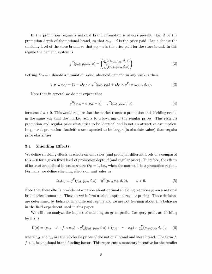
In the promotion regime a national brand promotion is always present. Let d be the

promotion depth of the national brand, so that pnb − d is the price paid. Let s denote the

shielding level of the store brand, so that psb− s is the price paid for the store brand. In this

regime the demand system is

qP (pnb, psb, d, s) =

(qPnb(pnb, psb, d, s)

qPsb(pnb, psb, d, s)

)(2)

Letting DP = 1 denote a promotion week, observed demand in any week is then

q(pnb, psb) = (1−DP )× qR(pnb, psb) +DP × qP (pnb, psb, d, s). (3)

Note that in general we do not expect that

qR(pnb − d, psb − s) = qP (pnb, psb, d, s) (4)

for some d, s > 0. This would require that the market reacts to promotion and shielding events

in the same way that the market reacts to a lowering of the regular prices. This restricts

promotion and regular price elasticities to be identical and is not an attractive assumption.

In general, promotion elasticities are expected to be larger (in absolute value) than regular

price elasticities.

3.1 Shielding Effects

We define shielding effects as effects on unit sales (and profit) at different levels of s compared

to s = 0 for a given fixed level of promotion depth d (and regular price). Therefore, the effects

of interest are defined in weeks where DP = 1, i.e., when the market is in a promotion regime.

Formally, we define shielding effects on unit sales as

∆q(s) ≡ qP (pnb, psb, d, s)− qP (pnb, psb, d, 0), s > 0. (5)

Note that these effects provide information about optimal shielding reactions given a national

brand price promotion. They do not inform us about optimal regular pricing. Those decisions

are determined by behavior in a different regime and we are not learning about this behavior

in the field experiment used in this paper.

We will also analyze the impact of shielding on gross profit. Category profit at shielding

level s is

Π(s) = (pnb − d− f × cnb)× qPnb(pnb, psb, d, s) + (psb − s− csb)× qPsb(pnb, psb, d, s), (6)

where cnb and csb are the wholesale prices of the national brand and store brand. The term f ,

f < 1, is a national brand funding factor. This represents a monetary incentive for the retailer

8

to actually run the national brand price promotion and corresponds to a lower wholesale price

on any units sold in the promotion week. We can calculate (6) at different shielding levels to

obtain the effects on category profits. The shielding impact on profits is a complex function

of relative margins between the national brand and store brand in the promotion week and

of the substitution patterns in the demand system.

In the next section we discuss the importance of shielding effects for the retailer and the

identification of shielding effects from historical data.

4 Identifying Shielding Effects from Historical Data

The data used in this paper comes from a national chain of convenience stores that sell a

typical array of private label and national brand products in the grocery, health and beauty

and general merchandize categories. This chain has a very large number of store locations

throughout the United States with most concentration in the Midwest and East Coast region.

In our analysis we use data for 28 products. For reasons of confidentiality we do not disclose

the specific product names. A general classification of the types of product categories used

is given in Table 1 along with the index used in the data analysis. For each of these products

we have unit sales and price data at the store level for the leading national brand and the

corresponding “copy-cat” store brand for 30 weeks. In addition, we have cost data for both

the national brand and the store brand. Summary statistics on the products are discussed

below.

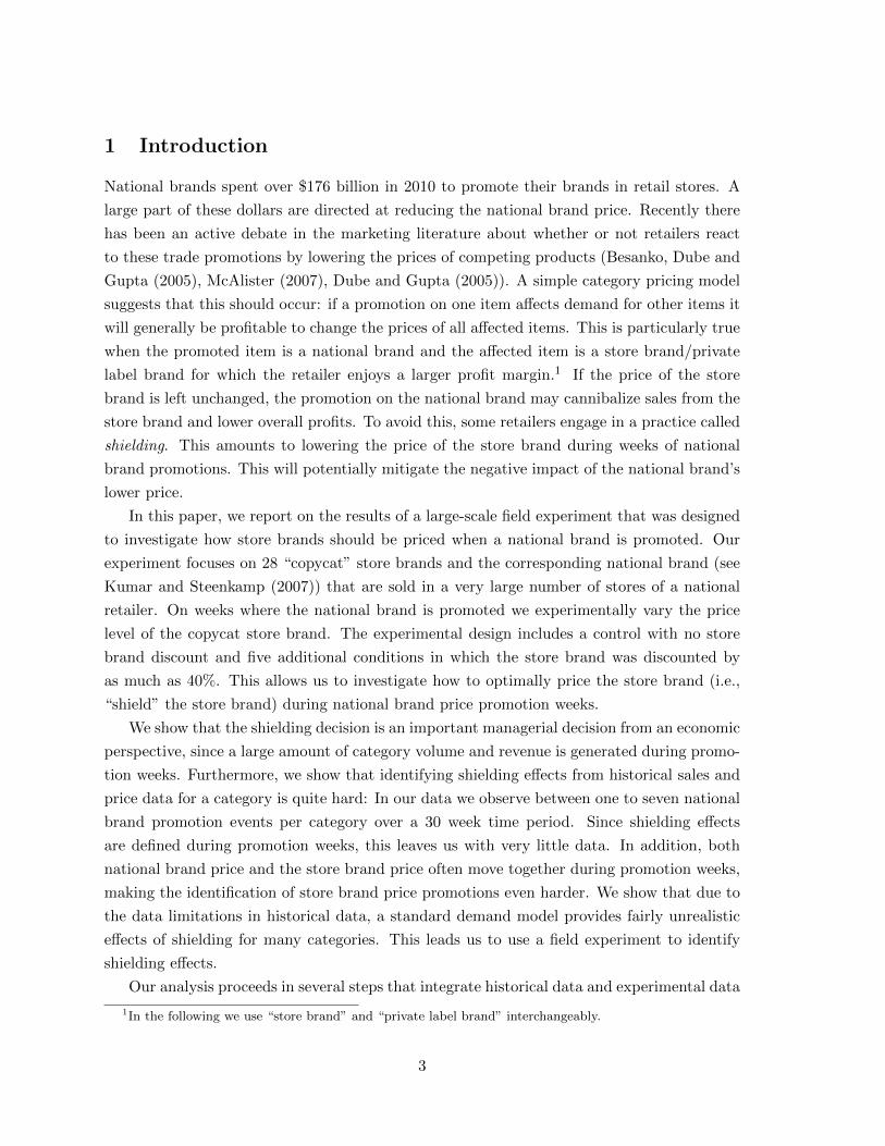
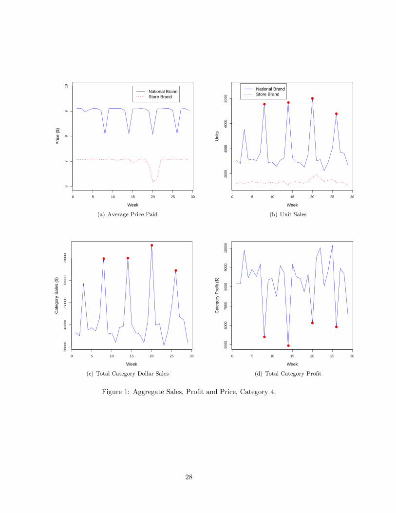
We start by illustrating the managerial importance of studying shielding effects. Fig.1(a)

shows the average price paid for the national brand (and store brand) over time for one of the

product categories in our data. The national brand had four promotions over the observation

period – these took place in week 8, 14, 20 and 26.3 Not surprisingly, these promotions gen-

erated a substantial lift in unit sales of the national brand (Fig.1(b)). While this is clearly

beneficial for the manufacturer of the national brand, the retailer cares primarily about cat-

egory impact, e.g., category revenue and profit. The national brand price promotion has

two effects on category profits. First, the national brand price promotion leads to a direct

decrease in the retailer’s margin for the national brand. Depending on the size of the price

elasticity, this may either increase or decrease the national brand’s contribution to category

profit. Second, the national brand price promotion makes the national brand increasingly at-

tractive to customers compared to the store brand. This raises the probability that customers

will substitute towards the national brand. This second effect is very problematic for the re-

tailer: In non-promotion weeks, the store brand’s margin is already much higher than the

3This plot shows data for the first 29 weeks of the 30 week observation period. In fact, the was a fifth

national brand promotion in the 30th week, but for reasons that will become apparent below we have not

included this data point in the plots.

9

national brand. In promotion weeks this discrepancy is even higher. For the product shown

in Fig.2, the national brand’s margin is already 75% lower than the store brand margin in

non-promoted weeks. In weeks where the national brand is on promotion the corresponding

number is an astounding 98%. The substitution from a high margin product to a low margin

product will lead to an unambiguous negative contribution to category profit. In Fig.1(d) we

see that the overall effect is a substantial decrease in category profits in the promoted weeks.

In order to mitigate the loss in category profits arising from the national brand’s price

promotion, the retailer may try to shield the store brand. In fact, looking at Fig.1(a), we can

see that for this category the retailer did this for the promotion in week 20. This makes the

store brand relatively less unattractive than it would otherwise be. This also means that the

effect we see on category profits in Fig.1(d) in week 20 is smaller than it would have been had

the retailer not shielded the store brand in that week. A couple of natural questions to ask

are then: what is the true effect of shielding? what is the optimal amount of shielding? which

factors determine the optimal amounts of shielding? A quick glance at Fig.1 reveals that these

are not trivial questions to answer. The only data points informative about shielding effects

are national brand promotion weeks (at least without making further assumptions about the

demand structure in the market). This gives us four data points for this category. However,

even these four observations are not very informative about the effects of shielding: We only

have one observation in the data where the retailer actually is observed to shield the store

brand – in the other three weeks there is no shielding. This leaves us with essentially two

observations on which to estimate an effect. It is simply not possible to learn much about

shielding effects from this. What we need is variation in the shielding level, conditional on a

national brand price promotion.

Table 2 demonstrates that the difficulty in identifying effects of shielding from historical

data is not unique to the category shown in Fig.1: For the 28 categories in our data, the

number of national brand promotion weeks ranges from 1 to 8, with an average of 4.1. So – on

average – we have about four observations per category on which to identify shielding effects.

The average depth of the national brand promotion across categories is around 20% with a

minimum of 11% and maximum of 31%. Table 2 also shows that the variation in store brand

price during national brand promotion weeks is small for many categories. About a third

of the categories have essentially no variation in store brand price during promotion weeks.

The table also demonstrates that for the overwhelming majority of categories, total category

sales volume is significantly higher during promotion weeks. Since all categories (except for

one) have substantially higher store brand margins compared to national brand margins, this

increased volume in weeks where customers substitute to the low margin brand underlines

the general managerial problem induced by the national brand promotion. Overall, Table 2

underlines that this is an important issue to retailers and that without further information

or assumptions, the historical data cannot precisely identify the effects of shielding, let alone

10

tell us what the optimal amount of shielding is.

4.1 A Demand Model

Recall from above that we defined shielding effects as the effects of lowering the store brand

price conditional on a national brand price promotion. There are at least two ways in which

we can learn about the size of shielding effects. One is simply to look at the observed

historical variation in the store brand price during national brand promotion weeks and then

compare this to changes in demand. The section above showed that this variation is too

small and infrequent to reliably estimate any effects. An alternative approach is to use the

entire observation period including both non-promotion and promotion weeks to estimate a

demand model and then infer shielding effects from the estimated demand model. Note that

this approach assumes that the observed price changes (and associated changes in demand)

between promotion and non-promotion weeks are informative about shielding effects and,

therefore, must assume some version of condition (4). It should be clear that this requires

that we put a fair amount of trust in the estimated demand model, since in the historical

data, we observe either no shielding or shielding at a generally constant level. In order to

believe in the shielding effects derived from the demand model, we have to assume that

the model holds up to extrapolation into a data range not observed in the historical data.

In contrast to Section 3, we are here assuming a “one-regime” world for the structure of

demand: The only difference between promotion and non-promotion weeks are changes in

prices, and this assumption allows us to pool data for the promoted and non-promoted weeks.

The formulation and estimation of a stable demand model is, of course, a fairly conventional

thing to do in both marketing and economics. However, as we will demonstrate below, this

approach is poorly suited as a general methodology for identifying shielding effects.

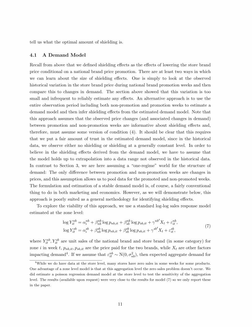
To explore the viability of this approach, we use a standard log-log sales response model

estimated at the zone level:

log Y nbit = αnbi + βnbnb log pnb,it + βnbsb log psb,it + γnb

′Xt + εnbit ,

log Y sbit = αsbi + βsbnb log pnb,it + βsbsb log psb,it + γsb

′Xt + εsbit ,

(7)

where Y nbit , Y

sbit are unit sales of the national brand and store brand (in some category) for

zone i in week t, pnb,it, psb,it are the price paid for the two brands, while Xt are other factors

impacting demand4. If we assume that εnbit ∼ N(0, σ2nb), then expected aggregate demand for

4While we do have data at the store level, many stores have zero sales in some weeks for some products.

One advantage of a zone level model is that at this aggregation level the zero sales problem doesn’t occur. We

did estimate a poisson regression demand model at the store level to test the sensitivity of the aggregation

level. The results (available upon request) were very close to the results for model (7) so we only report these

in the paper.

11

the national brand is

Qnb(pnb, psb) =

6∑i=1

exp{αi + βnbnb log pnb + βnbsb log psb + γnb

′X +

1

2σ2nb

}. (8)

A similar equation holds for the store brand.

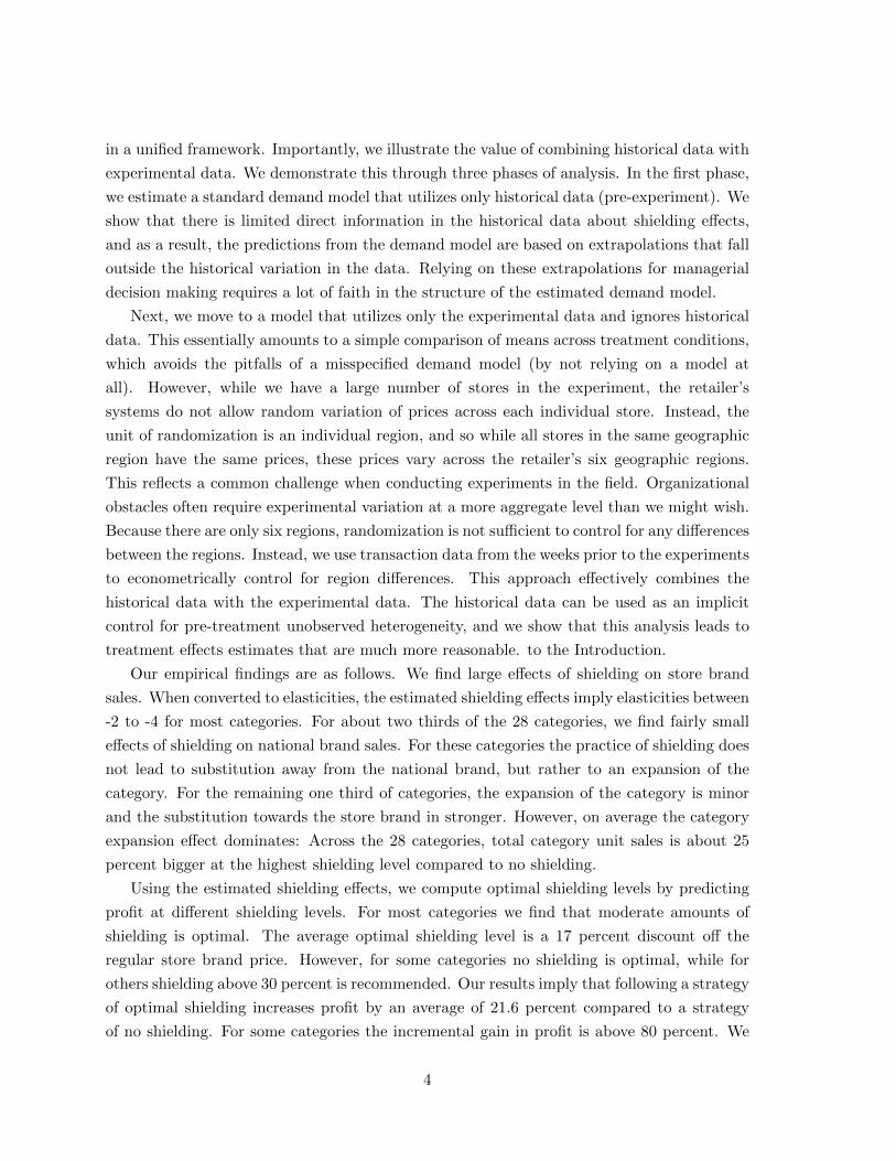
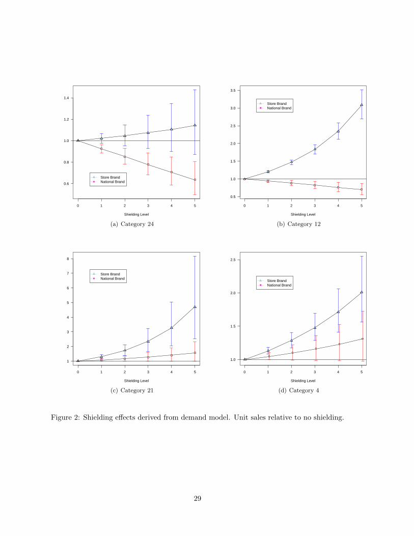
We estimated the parameters of (7) and computed shielding effects based on (8).5 Fig.

2 shows the estimated shielding effects for four of the over-the-counter medicine categories

in the data. The effects were computed based on national brand promotions of depth 20%,

32%, 29% and 16%, respectively for Fig.2(a)-2(d). Each sub-figure shows shielding effects

on the store brand and national brand relative to the no-shielding condition (labeled “0”).

The shielding levels were varied from very low (shielding level 1) to very high (level 5). For

shielding level 1 the store brands were shielded by 7%, 8%, 6% and 5%, respectively. Shielding

at the highest level was set at 33%, 39%, 30% and 27%.6 Fig.2(a) shows that shielding the

store brand in category 24 leads to only moderate increases in the demand for the store

brand compared to no shielding. The highest shielding level leads to an increase in unit sales

of the store brand relative to no shielding of around 10 percent (although this effect is not

estimated precisely). However, the shielding effects on the national brand are much larger.

The lowest level of shielding leads to a decrease in sales of the national brand compared to

no shielding of 8 percent. The highest level of shielding leads to a decrease of almost 40

percent. For this category shielding causes the national brand promotion to be much less

effective in terms of national brand sales, but has little impact on store brand sales. For

category 12, this pattern is reversed: Shielding has very large effects on store brand sales

(the effect is close to 200 percent at the highest shielding level), but fairly small effects on

national brand sales. In these categories the signs of the effects are what we would expect.

The remaining two categories are more troubling. For these categories shielding actually

increases demand for the national brand compared to no shielding. This is hard to explain.

In addition, the effects on the store brand in category 21 appears unrealistically large. This

illustrates part of the problem with identifying shielding effects using the historical data in

conjunction with a demand model: We showed above that the retailer historically has either

not shielded the store brand or only shielded it at lower levels. Therefore we are forced to

rely on extrapolation of a parametric demand model to inform us about shielding. Based on

Fig.2(b) and 2(d) there is some indication that this leads to unrealistic effects both in terms

of sign and magnitude.

5We estimated the model using a standard Gibbs sampling algorithm with proper but non-informative

priors on all parameters. We estimated both a “shrinkage” version where it was assumed that αi ∼ N(µ, τ)

with a prior on µ and τ , and a non-shrinkage version where the αi’s were given independent normal priors

with wide dispersion. The results were very similar and we show only the results for the shrinkage version.

Details on the estimation procedure is available from the authors upon request.6The reason for the choice of these specific numbers will be explained below.

12

We recognize that in our historical analysis, we only have access to 30 weeks of data. Many

published studies consider 1-2 years of historical data, which is an additional 20-70 weeks.

This additional data will clearly provide many more weeks in which the national brand is

promoted. If we extrapolate from our average of 4 promotion events in our data, we may

expect to observe 2-9 more promotion events with a longer time series. Note, however, that

this is unlikely to address the problems that we identified above. If we rely on the promotion

weeks to identify shielding effects, we still require variation in the store brand price during

those weeks. We have already shown that this variation is quite limited.

5 Field Experiment

Above we showed that identifying shielding effects through historical data and a demand

model was problematic for some products. In this section we will take another approach. In

collaboration with the retailer, we implemented a field test where shielding levels were varied

experimentally throughout the entire retail chain. The field test focused on 28 national brand

promotions. The promotions each lasted one week, and occurred over five contiguous weeks

in February and March 2008. The data we used above consisted of the 29 weeks prior to the

experiment. During the promotion weeks the prices of the national brands were temporarily

reduced, and these discounts were highlighted in the retailers’ weekly advertising and at the

point of sale. The 28 promotions were selected for the test because the retailer offered private

label items that competed directly with these national brands.

The design of the field test included six experimental conditions. These included a “no

shielding” condition, in which the price of the store brand was left unchanged (at its regular

price level) during the week that the national brand was promoted. In the other five conditions

the prices of the store brand were discounted during the promotion week. The depth of the

discounts varied across the five conditions, depending upon the regular price of the store

brand, with bigger discounts on SKUs that had higher regular prices. The actual price

treatments are summarized in Table 3.

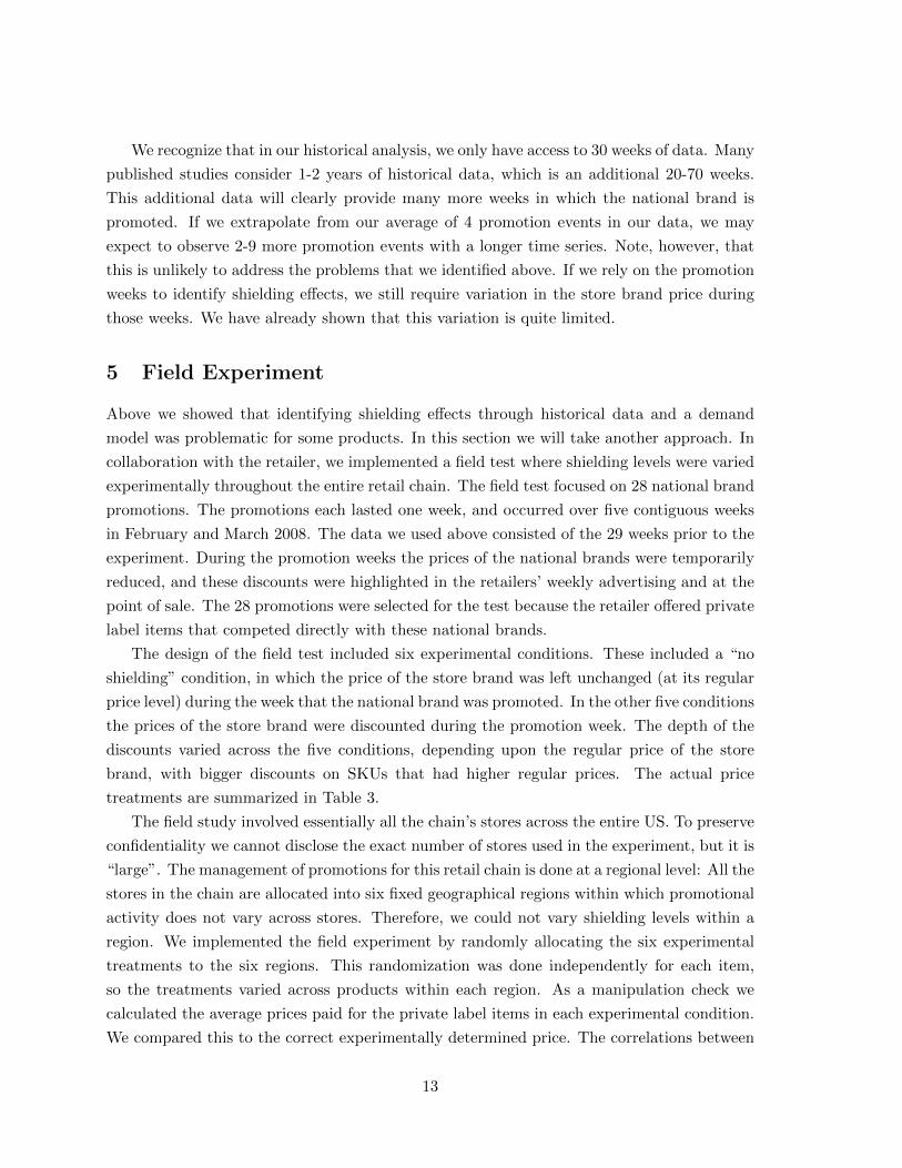
The field study involved essentially all the chain’s stores across the entire US. To preserve

confidentiality we cannot disclose the exact number of stores used in the experiment, but it is

“large”. The management of promotions for this retail chain is done at a regional level: All the

stores in the chain are allocated into six fixed geographical regions within which promotional

activity does not vary across stores. Therefore, we could not vary shielding levels within a

region. We implemented the field experiment by randomly allocating the six experimental

treatments to the six regions. This randomization was done independently for each item,

so the treatments varied across products within each region. As a manipulation check we

calculated the average prices paid for the private label items in each experimental condition.

We compared this to the correct experimentally determined price. The correlations between

13

actual prices paid and the experimental price within product ranged from 96% to 100%. We

also calculated the average deviance across conditions between prices paid and the experiment

price as a percent of the experimental price7. The average deviance was 4% and except for

two products out of the total 28 products these deviances were all below 6%. In light of the

significant logistical challenge of implementing a price test of this scale, we conclude that the

field experiment was implemented successfully.

In the next section we discuss the identification of the shielding effects using the field

experiment.

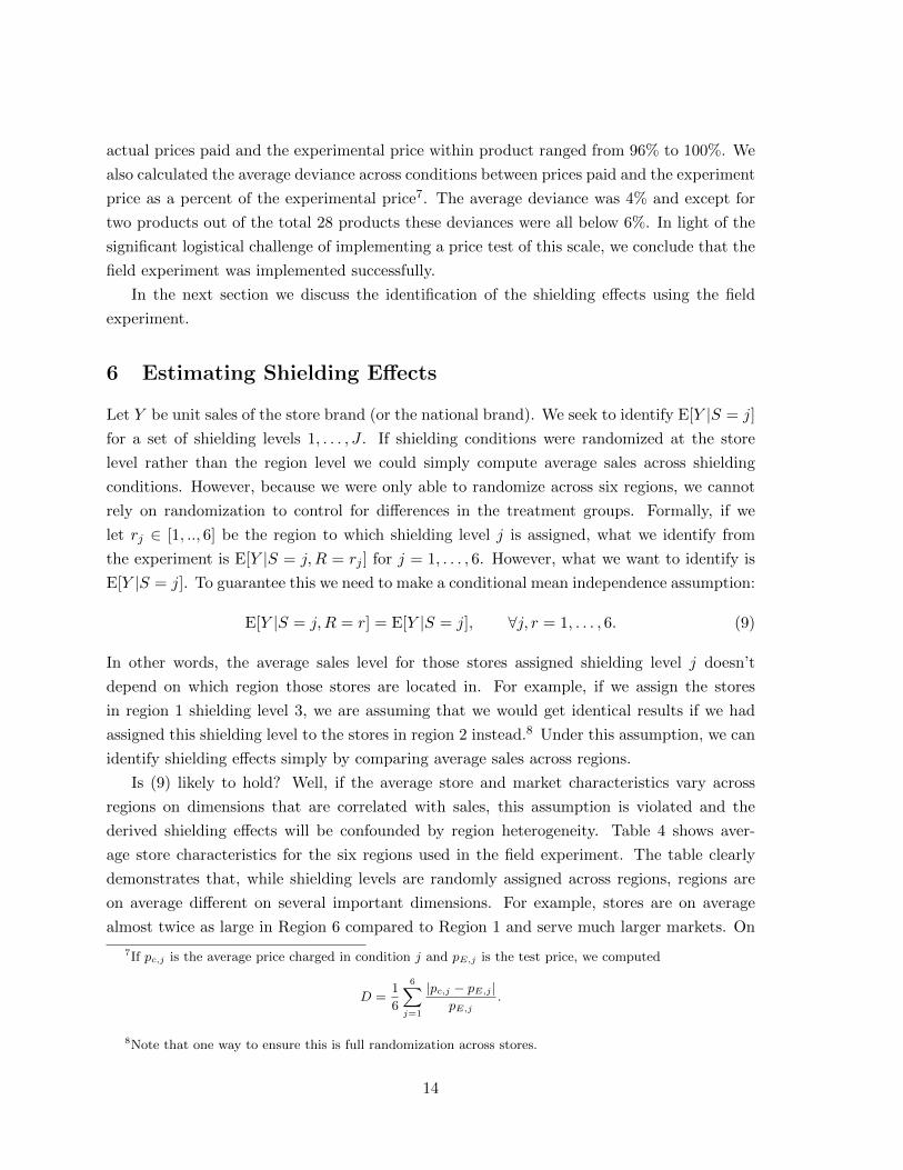
6 Estimating Shielding Effects

Let Y be unit sales of the store brand (or the national brand). We seek to identify E[Y |S = j]

for a set of shielding levels 1, . . . , J . If shielding conditions were randomized at the store

level rather than the region level we could simply compute average sales across shielding

conditions. However, because we were only able to randomize across six regions, we cannot

rely on randomization to control for differences in the treatment groups. Formally, if we

let rj ∈ [1, .., 6] be the region to which shielding level j is assigned, what we identify from

the experiment is E[Y |S = j, R = rj ] for j = 1, . . . , 6. However, what we want to identify is

E[Y |S = j]. To guarantee this we need to make a conditional mean independence assumption:

E[Y |S = j, R = r] = E[Y |S = j], ∀j, r = 1, . . . , 6. (9)

In other words, the average sales level for those stores assigned shielding level j doesn’t

depend on which region those stores are located in. For example, if we assign the stores

in region 1 shielding level 3, we are assuming that we would get identical results if we had

assigned this shielding level to the stores in region 2 instead.8 Under this assumption, we can

identify shielding effects simply by comparing average sales across regions.

Is (9) likely to hold? Well, if the average store and market characteristics vary across

regions on dimensions that are correlated with sales, this assumption is violated and the

derived shielding effects will be confounded by region heterogeneity. Table 4 shows aver-

age store characteristics for the six regions used in the field experiment. The table clearly

demonstrates that, while shielding levels are randomly assigned across regions, regions are

on average different on several important dimensions. For example, stores are on average

almost twice as large in Region 6 compared to Region 1 and serve much larger markets. On

7If pc,j is the average price charged in condition j and pE,j is the test price, we computed

D =1

6

6∑j=1

|pc,j − pE,j |pE,j

.

8Note that one way to ensure this is full randomization across stores.

14

the other hand, customers living in Region 1 are on average more affluent than the other

regions. These summary measures indicate that direct comparison of sales and profit across

conditions might lead to very misleading estimates of shielding effects. Below we provide

direct empirical evidence of this.

6.1 Controlling for store heterogeneity

As documented above, the assumption in (9) needed for the validity of direct comparisons of

test conditions is unrealistic in our context. However, suppose we can find a set of observable

variables Z such that

E[Y |S = j, R = rj , Z = z] = E[Y |S = j, Z = z], j = 1, . . . , 6. (10)

This condition requires that we get the same average sales level if we assign shielding level

j to stores with Z = z located in region 1 (for example) as we would have if we instead

had assigned shielding level j to stores with Z = z in region 2 (for example). With this

assumption we can “condition our way out” of the problem of regions being heterogenous

before the experiment. As long as we can find enough stores in different regions with the

same Z = z, we can calculate shielding effects for this segment of stores. Average effects can

then be calculated by weighted averages of the Z distribution.

Under assumption (10) and access to enough data we can control for store heterogeneity

by simply defining treatment cells very finely.9 However, when Z is high dimensional an

abnormally large amount of data is required for a full non-parametric approach10. An al-

ternative approach is to match stores across conditions using Rosenbaum-Rubin Propensity

Score Matching (cf., Rosenbaum and Rubin (1983)). However, this approach is not easy

to implement in situations with more than one treatment due to the need for identifying

matched stores across all conditions.

Overall, assumption (10) is clearly preferable to (9). However, it does require that there

are no remaining unobservable store or market characteristics that vary across regions and

are correlated with sales. In relying on (10) we have to feel confident that we have conditioned

on all information that may cause pre-experiment heterogeneity in sales. In the next section

we show how we may use historical sales data at the store level to control for unobservable

heterogeneity in sales.

9For example, if region heterogeneity was contained to store size only, we could simply compute effects for

different sizes, e.g., small, medium and large stores.10Consider the following example. Suppose we only had three Z variables, each of which had four levels.

This gives us 12 cells and for each of these 12 cells we need to estimate 6 conditional means. This is a total

of 72 conditional means. This requires a large number of stores evenly distributed across all 72 groups.

15

6.2 Controlling for unobserved heterogeneity

Assumption (10) implies that the researcher observes all variables that cause pre-experiment

heterogeneity in sales across regions. This is a strong assumption. Suppose instead that we

decompose the Z vector into Z = (Z̃, Z∗), where Z̃ is an observed vector of covariates and Z∗

is a vector of unobserved covariates impacting sales. We assume that an augmented version

of (10) holds:

E[Y |S = j, R = rj , Z̃ = z̃, Z∗ = z∗] = E[Y |S = j, Z̃ = z̃, Z∗ = z∗], j = 1, . . . , 6. (11)

Note that this is a much less restrictive assumption than (10), since we are now assuming

the existence of some unobservable heterogeneity vector such that conditional on it (and

other observable covariates), mean sales at some shielding level j does not depend on which

region is assigned that shielding level. Clearly, (11) is not of much direct use in terms of

non-parametric estimation, since we can only condition on what we can observe. Therefore,

we can ask what would happen if (11) is true, but we assume that (10) holds:

E[Y |S = j, R = rj , Z̃ = z̃] = E[Y |S = j, Z̃ = z̃], j = 1, . . . , 6. (12)

Under what condition is (12) true, if (11) is true? It is straightforward to show that this

requires that the distribution of unobserved heterogeneity Z∗ conditional on Z̃ is identical

across regions. Again, this seems like a very strong assumption.

To accommodate unobservable heterogeneity without assuming the distribution of it is

identical across regions, we will rely on historical sales data at the store level. This allows us

to control for time invariant unobservable heterogeneity in sales without requiring (12). The

price we must pay for this is a required assumption on the dimensionality of unobservable

heterogeneity and the specific way it impacts both historical sales and sales in the test week at

the store level. As mentioned above, we are doing this because we were only able to randomize

at the region level rather than the store level. If it was, each experimental condition would

consist of stores with similar observable and unobservable heterogeneity and we could simply

compare average outcomes across conditions. Our empirical approach will correct for the fact

that this is not the case.

Contrary to the demand model estimated in Section 4, we now need to analyze the data

at the store level.11 A complicating factor of the store level data is that unit sales at the

store level are typically quite small for most stores. Many stores have zero sales in several

weeks for some categories. This makes use of a linear or log linear model impossible. To

11Since treatments only vary at the region level, analysis at the region level would give us only one observation

per treatment.

16

accommodate zero sales observations, we will use a Mixed Poisson regression model:

Y sbit ∼ Poi(λsbit ), t = 1, . . . , T ; i = 1, . . . , N,

log λsbit ∼ N(αsbi + βsbnbDnb,t + βsbsbDsb,t + γsb

′Xt +

L∑l=1

βsbl Dilt, 1/τsbt

),

αsbi ∼ N(µsbα , 1/τsbα ),

(13)

where Y sbit are unit sales of the store brand for store i in week t for a product category,

αsbi captures unobservable heterogeneity for store i, Dnb,t(Dsb,t) is one if the national brand

(store brand) is promoted in week t, Xt are other time varying factors impacting sales and

Dilt = 1 in the test week if shielding level l is assigned to store i. Assigning a distribution

of λsbit allows for overdispersion of zeros compared to a standard Poisson regression model.

The store brand and national brand promotion dummies enable us to get a clean estimate

of αi using historical sales data. In the empirical specification used below, Xt consists of a

quadratic trend since some categories exhibit general increasing or decreasing sales over the

observation period. We estimate a model similar to (13) for national brand sales. This allows

us to estimate shielding effects on overall category profit12. From (13) we can derive both

store level and aggregate shielding effects for store brand and national brand sales as well as

category profits.

7 Results

7.1 Mean Comparisons

We start by illustrating the importance of controlling for pre-experiment heterogeneity when

dealing with a field experiment where the unit of randomization is at an aggregate level. In our

case, there are a large number of stores, but the randomization is at the region level, yielding

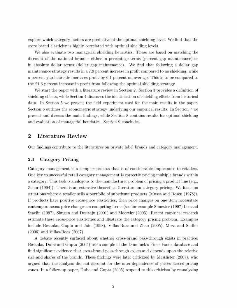
just six treatment groups. Fig.3 shows shielding effects based on simple mean comparisons

of store brand sales across test cells (i.e., regions) for two of the 28 categories. The figures

compares unit store brand sales across shielding levels normalized by a benchmark of no

shielding (denoted by shielding level 0). We would expect store brand sales to be increasing

in the shielding level, but this is not what we see. For example, for the first category we see

that shielding at the lowest level (shielding level 1) increases sales by 100 percent compared

to no shielding, while shielding at the next level (level 2) reduces sales back to the benchmark

level. Sales then increase moderately at the higher shielding levels. The shielding effects are

12We estimate the model using a Markov Chain Monte Carlo algorithm. The precision parameters

τsbt , τα, τnbt are given Gamma priors with a mean of 1 and variance of 50. The remaining parameters are

given normal priors with mean zero and variance of 100. Details on the estimation procedure can be obtained

from the authors upon request.

17

even more absurd for the second category where sales first increase with shielding and then

fall at the highest level of shielding. These results are not surprising in light of the large

differences across regions shown in Table 4. A result of this is that when we are comparing

sales outcomes across shielding levels we are not on average “holding everything else fixed”.

This highlights the need for controlling for store heterogeneity in the current context since

we cannot rely on randomization to do the job for us.

7.2 Controlling for unobservable heterogeneity

We estimated the model in (13) separately for both store brand sales and national brand

sales. Table 5 and 6 shows the estimated coefficients for store brand sales. Except for a

few categories, the estimated signs and sizes are as expected. In 22 out of 28 categories, the

βsbnb parameter is negative implying that national brand promotions lower sales of the store

brand. For example, for category 1, the posterior mean estimate of the parameter is -0.23,

which translates to a 20.5 percent decrease in the mean of the implied Poisson distribution.

We also see large positive effects of store brand promotions in the historical period (βsbsb) for

26 out of 28 categories. Again, for the first category, the estimated parameter translates to

a 39 percent increase in store brand sales.

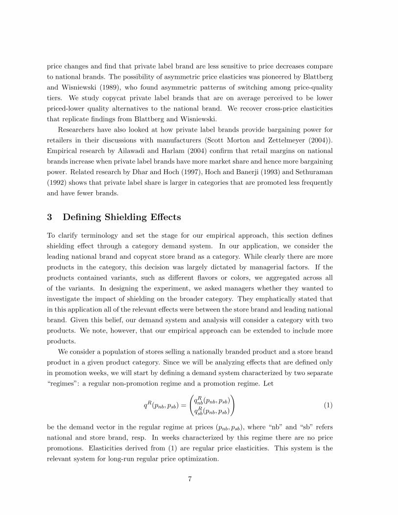
The shielding effects are captured by the parameters βsbl , l = 1, . . . , 6. While there is a

lot of variation across categories, in general, the signs and magnitudes make sense: Shielding

matters and higher levels of shielding are consistent with higher store brand sales. Note that

the total impact on store brand sales in the test week is the sum of the impact of the national

brand promotion (βnb) and the shielding coefficient βsh,j (since shielding is done in the same

week as the national brand promotion). Fig.4 plots the posterior mean estimates of this

sum for all 28 categories along with the average for all categories (represented by the solid

line). Not surprisingly, most categories display a negative impact with no shielding. Even

shielding at the lowest level (level 1) results in a negative impact on store brand sales for

most categories. At shielding level 2 we see that – on average across the 28 categories – the

national brand promotion has been off-set by shielding the store brand. At the highest level

of shielding, all categories (except for one) have increased store brand sales compared to no

shielding.13

To show that the model in (13) leads to much more reasonable shielding effects compared

to simple mean comparisons, Fig.5 shows implied shielding effects for the same two categories

shown in Fig.3. As expected from theory, the shielding effects on store brand sales are

increasing in shielding level. Category 1 shows very large effects with a 200 percent increase

in store brand sales at the highest shielding level compared to no shielding. The second

13For readability reasons we have not included measures of parameter uncertainty in Fig.4. Also note that

it is somewhat misleading to average parameters across categories since the percentage changes in shielding

levels are not identical across categories.

18

category shows more moderate effects with an about 25 percent increase in store brand sales

at the highest shielding level.

To summarize and compare the estimated shielding effects for all 28 categories, we com-

pute the implied shielding elasticities. Since we have not imposed a constant elasticity re-

striction on the model, the shielding elasticity will in general vary with store brand price

value. To provide a parsimonious measure of shielding elasticity, we compute the average

elasticity across the prices used in the experiment:

ε̄(θ) =1

5

5∑j=1

εj(θ), (14)

where εj is defined as

εj(θ) =

qj+1(θ)−qj(θ)(qj+1(θ)+qj(θ))/2

pj+1−pj(pj+1+pj)/2

, j = 1, . . . , 5, (15)

and p1 > p2 > · · · > p6 are the store brand test prices, qj(θ) is predicted aggregate sales

derived from (13) when the national brand promotion dummy is one, the dummy for store

brand shielding at level j is one, and θ denotes the parameter vector.14 Fig.6(a) shows the

estimated shielding elasticities on store brand sales for all 28 categories. The majority of the

estimated elasticities fall in the minus 2 to minus 4 range. One category has an elasticity

close to zero and several are less than in one in absolute value. As mentioned above we also

estimated the model for national brand sales. Fig.6(b) shows the estimated cross shielding

elasticities on national brand sales. These are much smaller, falling primarily in the -0.5 to

0.5 range. Together Fig.6(a) and (b) indicate that shielding the store brand will for most

categories lead to a lift in store brand sales, but only minimal changes in national brand

sales. To complete the visual representation of the full 2× 2 cross-price elasticity matrix, we

also computed implied price elasticities for the national brand price.15 These are shown in

Fig.6(c) and 6(d). We see that the national brand price elasticities on store brand sales are, in

general, much larger than the other reverse cross price elasticity (in Fig.6(b)) with about half

of the categories having elasticities bigger than 1. The national brand’s own price elasticity

is also substantial with most categories having elasticities between -2 and -6. Overall, the

results in Fig.6 can be taken to corroborate the asymmetric “price-tier” finding in Blattberg

14While ε̄(θ) has the advantage of capturing price sensitivity with just one number, it will be somewhat

misleading if there are large changes in price elasticity across the demand curve. Note also that ε̄(θ) is a

not a standard price elasticity – it is a pass-through elasticity. In other words, it measures the sensitivity to

discounting the store brand conditional on a discount of the national brand.15Since we only have a dummy representing a national brand price promotion in the model, we computed

the price elasticities by comparing the incremental in sales implied by the dummy coefficient to the average

size of the national brand price promotion in the sample.

19

and Wisniewski (1989): Promotions for the high priced brand impacts the lower priced brand,

but the reverse effect is much smaller.

7.3 Comparison to Demand Model

To compare our estimated shielding effects to those obtained from a more conventional ap-

proach, we can contrast the estimates using the field experiment to the ones obtained for

the demand model in Section 4 using only the historical data. Both approaches yield predic-

tions about the effects of shielding, but they do so from two very different perspectives. The

demand model (7) embodies a certain “stationarity” assumption about market responses to

price changes. In particular, as we change pnb and psb it is assumed that we can extrapolate

the effects by relying on the parameter values and functional form in (7). In other words, (7)

is assumed to be a structural model.16 Thus, we are relying on historical price variation to

estimate the parameters in (7) and assuming that the same functional form and parameter

values can be used to predict shielding effects. This is very different from the specification

in (13), which is simply a statistical model used to correct for the fact that we were only

able to randomize at the region level (rather than the store level). Ideally, we would just

have calculated mean comparisons to obtain shielding effects for the experiment, which would

make the contrast to (7) even stronger.

Fig.7 compares the estimated effects using the field experiment to those obtained from

the model above for the same four categories shown in Fig.2. We focus on the effects on store

brand sales. For category 24 we see that the model vastly underestimates the effects from

the field experiment, while for category 21 the model hugely overestimates the experimental

effect. For category 12 we see that for the lowest amounts of shielding, the model results are

close to the field experiment, but the model does not capture the drop-off in effect size at the

highest shielding levels. Finally, for category 4 the estimated effects are largely similar.

7.4 Decomposing Effects of Shielding

We argued in the introduction that the main objective of shielding is to drive demand away

from the promoted (national) brand towards the higher margin (store) brand. However, the

elasticities shown in Fig.6 indicated that the shielding effects on national brand sales were

relatively small. To expand on this finding, Fig.8 shows the average shielding effects on sales

of both the national and store brand as well as total category sales (i.e., the sum of the two

16It has become commonplace in empirical marketing to refer to “structural models” as models that are

derived from first principles, i.e., utility or profit maximization. However, originally, a structural econometric

model was an empirical model whose basic formulation (i.e, parameters and functional form) was assumed

invariant to certain changes in the exogenous variables. This is the definition we are using here (see Heckman

and Vytlacil (2007)).

20

brands). This figure clearly illustrates that – on average across the 28 categories – shielding

does not drive sales away from the national brand. We do see a small decline in national

brand sales, but, more importantly, we see a huge increase in sales of the store brand as

the shielding level increases. This large increase leads to a category expansion effect: Total

category sales are on average about 25 percent larger at the highest shielding level compared

to no shielding. This cannot be explained by a pure substitution effect away from the national

brand. Shielding does increase sales of the store brand dramatically, but not at the cost of

national brand sales.

To see that the effect in Fig.8 is an average over a set of more nuanced effects, Fig.9

shows shielding effects on unit sales for two individual categories. For the category in Fig.9(a)

shielding induces primarily a substitution effect: Overall category sales are flat and shielding

serves to crowd out national brand sales by shifting demand towards the store brand. This is

a category where the cross-brand elasticity matters. In Fig.9(b) shielding leads to a category

expansion effect. Here the shielding effects are closer to the average effects shown in Fig.8

where national brand sales is largely unaffected by shielding. For this category the cross-

brand elasticity is minor.

To get an overall sense of which effect dominates for all the 28 categories, Fig.10 plots the

cross-brand elasticity, category elasticity and the store brand own price elasticity (indicated

by the size of the points in the plot). Categories located near the horizontal line are categories

with no category expansion. Roughly one third of the 28 categories can be said to have very

little to no category expansion and these tend to be those categories with the biggest cross-

brand elasticities (the “north-east” region of the plot). The remaining categories have large

category expansion effects and – in general – these tend to have small cross-brand elasticities

and large store brand own price elasticities.

Can we explain what type of categories have large cross price elasticities? Fig.11 plots

the cross price elasticity versus the relative price of the national brand and the relative size

of the store brand. We see that the there is tendency for bigger cross price elasticities the

smaller the price gap is between the two brands. We also see that that the bigger the store

brand is compared to the national brand, the bigger is the cross price elasticity. Both of these

findings have intuitive appeal: In categories where the store brand is popular and priced close

to the national brand, we see the biggest cross-price effects of shielding. One interpretation

of this is that these are categories where the copy-cat store brand is of comparable quality

and therefore constitutes a viable substitute for the national brand.

8 Shielding: Optimality and Heuristics

In this section we use the estimated shielding effects to compute optimal shielding effects

and compare these to two types of manager heuristics. The two heuristics we evaluate are

21

“dollar gap maintenance” and “percent gap maintenance”. Under dollar gap maintenance

the manager reacts to the national brand discount by lowering the store brand price by an

equal dollar amount, while under percent gap maintenance the store brand’s price is lowered

by a percent equal to the percent discount in the national brand. Therefore, under price

gap maintenance the original dollar price gap between the national brand and store brand

is preserved, while under percent gap maintenance the original price gap in percent between

the national brand and store brand is preserved.17

We will evaluate the two heuristics by comparing them to the optimal level of shielding.

To compute optimal shielding, we first define category profits as

Π(s; θ) = (pnb − d− f × cnb)× Q̄nb(s; θ) + (psb − s− csb)× Q̄sb(s; θ), (16)

where pnb, psb, cnb, csb are price and marginal cost for the national brand and store brand,

and Q̄nb(s; θ), Q̄sb(s; θ) are expected sales of the national and store brand at shielding level

s given the parameter vector θ (as derived from (13)). The factor f is the level of funding

the retailer receives from the manufacturer to run the promotion. This is observable data

provided to us by the retailer. For example, a funding factor of 0.90 implies that the level of

funding received from the manufacturer per unit sold amounts to 10 percent of the original

wholesale price.

We compute the optimal shielding level by maximizing the posterior expected profit con-

ditional on a given national brand price promotion d. In particular, we compute

Π̂(s) ≡ E[Π(s; θ)] =

∫Π(s; θ)p(θ|y)dθ, s = s1, . . . , s6, (17)

where p(θ|y) is the posterior distribution of θ. The optimal shielding level is the sj , j =

1, . . . , 6, that maximizes Π̂(s). In a similar fashion we can compute the posterior expected

profit of the two heuristics by simply evaluating the posterior expectation of (16) at the

relevant prices.

8.1 Optimal Shielding

To get a sense of the overall optimal level of shielding across categories, we computed the

optimal shielding as a percentage of the benchmark (no-shielding) store brand price. Fig.12

shows the result for all 28 categories. The recommended optimal shielding level is between

10 and 30 percent for most categories. The average optimal shielding level is 17 percent.

For three categories the recommended shielding level is zero. For five categories the optimal

shielding percentage is 30 percent or above. We conclude that for most categories it is optimal

to engage in shielding of the store brand during national brand promotions.

17It is easy to verify that if both the national brand and store brand is lowered by x%, then the price gap

measured in percent between the national brand and store brand is preserved.

22

The optimal shielding level is a complex function of the depth of the national brand

promotion, the level of funding provided by the manufacturer, the relative margins of na-

tional versus store brand and the cross price and own price shielding elasticities. Since these

factors are likely to interact with each other in explaining the optimal shielding level, it is

a non-trivial matter to break out how much each factor explains of the overall variation in

optimal shielding. Fig.13 shows simple scatter plots between optimal shielding and two of

these factors: The depth of national brand promotion in the test week( Fig.13(a)), and the

store brand shielding elasticity (Fig.13(b)). Fig.13(a) shows that while there is some ten-

dency for deeper national brand promotions to require deeper shielding, the relationship is

not strong and there are several outliers. For example, the three categories for which optimal

shielding is zero, have fairly large promotion depths (23, 29 and 33 percent). A clue as to why

this is can be seen from Fig.6(a): These three categories have three of the four smallest (in

absolute value) shielding elasticities shown in the figure (-0.05 ,-1.17 and -0.66). For these cat-

egories we cannot generate incremental lift in store brand volume by shielding. This suggests

that shielding elasticities may be quite important in determining optimal shielding. This is

confirmed in Fig.13(b) which shows a strong negative correlation between optimal shielding

percentages and shielding elasticities. This is an implication of the category expansion effect

of shielding documented above.

8.2 Model and Experiment revisited

In Fig.14 we plot the posterior expected profit for two categories for both the experiment

and model. For category 13 we see that the experiment and model based profit functions

share a common maximum. For this category both approaches indicates optimal shielding at

the second lowest level. On the other hand, for category 3 we see that the field experiment

indicates optimal shielding at the highest level of shielding, while the model based profit

function suggests a no-shielding strategy. This again illustrates the potential danger in only

relying on the fitted demand model.

8.3 Evaluating Heuristics

By definition, implementing the optimal shielding level will lead to the highest possible cat-

egory profit. How close can we get to this level by using a heuristic? To answer this we

computed the realized category profit from following the two heuristics defined above. We

also calculated the profit resulting from using a third heuristic: doing nothing. This amounts

to leaving the store brand price unchanged when the national brand is on promotion. We eval-

uate optimal shielding, dollar gap maintenance and percent gap maintenance by comparing

the profit from these strategies to the profit realized if no shielding is done.

Fig. 15 shows the profit for the three heuristics as a percent of the optimal shielding

23

profit. The categories have been plotted in order of the magnitude in incremental profit from

optimal shielding versus no shielding. We see that there are substantial gains to be made

from optimal shielding versus no shielding. On average a strategy of no shielding only leads

to a profit of 83.9 percent of the optimal profit. For several categories this number is less

than 70 percent. The figure also illustrates that for most categories, following a heuristic is

better than doing nothing. This is not true for all categories: For those categories where

little to no shielding is optimal, it is naturally better to do nothing than follow a heuristic

of matching the national brand price promotion. Following the dollar gap heuristic will on

average lead to a profit equal to 88.6 percent of the optimal shielding profit. For the percent

gap heuristic this number is 87.4 percent.

We can make an alternative evaluation of these strategies. Rather than comparing them

to the optimal shielding strategy, we can ask how much better the heuristics and the optimal

strategy is compared to doing no shielding. Table 7 contains a numerical summary of this

statistic. On average for the 28 categories, optimal shielding increases category profit by 21.6

percent compared to no shielding. There is considerable variation across categories as docu-

ment by the standard deviation of 19 percent, and the maximal benefit in any category is 86.9

percent. Following a dollar gap maintenance heuristic results in a 7.9 percent improvement

in profit compared to no shielding. For the percent gap heuristic this is 6.1 percent. Using

this metric, the suggested heuristics will on average give a manager about one third of the

full profit potential realized by following the optimal shielding strategy. This is not bad, but

this is an average. Table 7 (and Fig.15) demonstrates that for some categories the heuristics

perform worse than doing nothing. By construction this tends to happen in categories where

the optimal shielding level is small or zero.

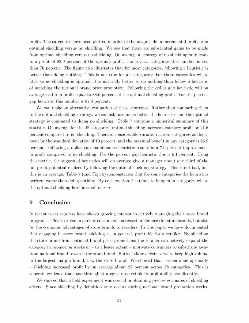
9 Conclusion

In recent years retailers have shown growing interest in actively managing their store brand

programs. This is driven in part by consumers’ increased preferences for store brands, but also

by the economic advantages of store brands to retailers. In this paper we have documented

that engaging in store brand shielding is, in general, profitable for a retailer. By shielding

the store brand from national brand price promotions the retailer can actively expand the

category in promotion weeks or – to a lesser extent – motivate consumers to substitute away

from national brand towards the store brand. Both of these effects serve to keep high volume

in the largest margin brand, i.e., the store brand. We showed that - when done optimally

– shielding increased profit by on average about 22 percent across 28 categories. This is

concrete evidence that pass-through strategies raise retailer’s profitability significantly.

We showed that a field experiment was crucial in obtaining precise estimates of shielding

effects. Since shielding by definition only occurs during national brand promotion weeks,

24

historical data has limited information about the effects of shielding on sales. We illustrated

this by estimating a standard demand model which led to effects that – for some categories

– differed quite dramatically from the experimentally derived effects. On the other hand,

we also argued that the field experiment itself was not enough to obtain reliable estimates

of shielding. A major obstacle to using field experiments are the logistical challenges in

randomizing treatments in actual markets. We established that merging historical price and

sales data with experimental evidence in a common econometric framework provided us with

the best of both approaches.

We readily admit to several caveats to the results in this paper. First of all, our products

are almost all drawn from the consumer health care and personal care product categories. It

is possible that we would get different findings in other product categories. Second, we did not

consider the dynamic effects of shielding. It is possible that post-promotion dynamic effects

would change the optimal shielding levels. Finally, all of our data was at the store level. We

do not have access to customer level data for the retailer that provided the data. However,

to develop a more detailed understanding of the substitution and category expansion effect,

it would be interesting to estimate shielding effects at the customer level. We leave this for

further research.

25

References

Ailawadi, K. and Harlam, B. (2004), ‘An empirical analysis of the determinants of retail

margins: The role of store-brand share’, Journal of Marketing 68(1), 147–165.

Besanko, D., Dube, J.-P. and Gupta, S. (2005), ‘Own-brand and cross-brand retail

passthrough’, Marketing Science 24, 123–137.

Besanko, D., Gupta, S. and Jain, D. (1998), ‘Logit demand estimation under competitive

pricing behavior: An equilibrium framework’, Management Science 44(11, Part 1), 1533–

1547.

Blattberg, R. and Wisniewski, K. (1989), ‘Price-Induced Patterns of Competition’, Marketing

Science 8(4), 291–309.

Cotterill, R., Putsis, W. and Dhar, R. (2000), ‘Assessing the competitive interaction between

private labels and national brands’, Journal of Business 73(1), 109–137.

Dhar, S. and Hoch, S. (1997), ‘Why store brand penetration varies by retailer’, Marketing

Science 16(3), 208–227.

Dube, J.-P. and Gupta, S. (2005), ‘Cross-brand pass-through in supermarket pricing’, Mar-

keting Science 27, 324–333.

Heckman, J. J. and Vytlacil, E. J. (2007), ‘Econometric evaluation of social programs, part i:

Causal models, structural models and econometric policy evaluation’, Handbook of Econo-

metrics, Vol.6b, Elsevier .

Hoch, S. and Banerji, S. (1993), ‘When do private labels succed?’, Sloan Management Review

34(4), 57–67.

Hoch, S. and Lodish, L. (1998), ‘Store brands and category management’, Working Paper,

The Wharton School .

Kumar, N. and Steenkamp, J.-B. E. (2007), Private Label Strategy, Harvard Business School

Press.

Lee, E. and Staelin, R. (1997), ‘Vertical strategic interaction: Implications for channel pricing

strategy’, Marketing Science 16, 185–207.

McAlister, L. (2007), ‘Cross-brand pass-through: Fact or artifact’, Marketing Science

pp. 876–898.

Meza, S. and Sudhir, K. (2006), ‘Pass-through timing’, Quantitative Marketing and Eco-

nomics 4(4), 351–382.

26

Moorthy, S. (2005), ‘A general theory of pass-through in channels with category management

and retail competition’, Marketing Science 24(1), 110–122.

Mussa, M. and Rosen, S. (1978), ‘Monopoly and product quality’, Journal of Economic

Theory 18, 301–317.

Raju, J., Sethuraman, R. and Dhar, S. (1995), ‘The Introduction and Performance of Store

Brands’, Management Science 41(6), 957–978.

Scott Morton, F. and Zettelmeyer, F. (2004), ‘The strategic positioning of store brands in

retailer-manufacturer negotiations’, Review of Industrial Organization 24, 161–194.

Sethuraman, R. (1992), ‘Understanding Cross-Category Differences in Private Label Shares

of Grocery Products’, Marketing Science Institute, Report No. 92128. .

Sethuraman, R. and Cole, C. (1999), ‘Factors influencing the price premiums that consumers

pay for national brands over store brands’, Journal of Product and Brand Management

(8), 340–351.

Shugan, S. and Desiraju, R. (2001), ‘Retail product-line pricing strategy when costs and

products change’, Journal of Retailing 77(1), 17–38.

Simester, D. (1997), ‘Optimal promotion strategies: A demand-sided characterization’, Man-

agement Science 43, 251–256.

Sivakumar, K. and Raj, S. (1997), ‘Quality tier competition: How price change influences

brand choice and category choice’, Journal of Marketing 61(3), 71–84.

Steenkamp, J.-B. E. M., Van Heerde, H. J. and Geyskens, I. (2010), ‘What Makes Consumers

Willing to Pay a Price Premium for National Brands over Private Labels?’, Journal of

Marketing Research 47(6), 1011–1024.

Villas-Boas, J. and Zhao, Y. (2005), ‘Retailer, manufacturers, and individual consumers:

Modeling the supply side in the ketchup marketplace’, Journal of Marketing Research

42(1), 83–95.

Villas-Boas, S. B. (2007), ‘Vertical relationships between manufacturers and retailers: Infer-

ence with limited data’, Review of Economic Studies 74(2), 625–652.

Zenor, M. J. (1994), ‘The Profit Benefits of Category Management’, Journal of Marketing

Research 31(2), 202–213.

27

0 5 10 15 20 25 30

67

89

10

Week

Pric

e ($

)

National BrandStore Brand

(a) Average Price Paid

0 5 10 15 20 25 30

2000

4000

6000

8000

Week

Uni

ts

●●

●

●

National BrandStore Brand

(b) Unit Sales

0 5 10 15 20 25 30

3000

040

000

5000

060

000

7000

0

Week

Cat

egor

y S

ales

($)

● ●

●

●

(c) Total Category Dollar Sales

0 5 10 15 20 25 30

5000

6000

7000

8000

9000

1000

0

Week

Cat

egor

y P

rofit

($)

●

●

●

●

(d) Total Category Profit

Figure 1: Aggregate Sales, Profit and Price, Category 4.

28

0 1 2 3 4 5

0.6

0.8

1.0

1.2

1.4

Shielding Level

Store BrandNational Brand

(a) Category 24

0 1 2 3 4 5

0.5

1.0

1.5

2.0

2.5

3.0

3.5

Shielding Level

Store BrandNational Brand

(b) Category 12

0 1 2 3 4 5

1

2

3

4

5

6

7

8

Shielding Level

Store BrandNational Brand

(c) Category 21

0 1 2 3 4 5

1.0

1.5

2.0

2.5

Shielding Level

Store BrandNational Brand

(d) Category 4

Figure 2: Shielding effects derived from demand model. Unit sales relative to no shielding.

29

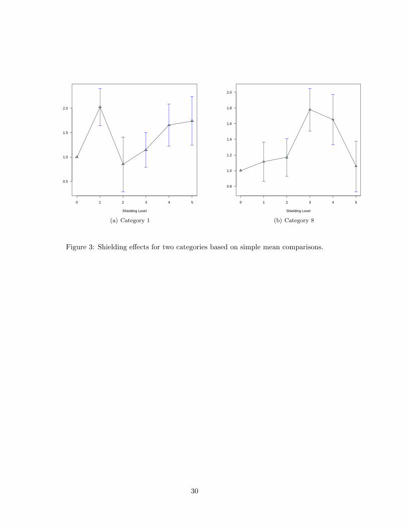
0 1 2 3 4 5

0.5

1.0

1.5

2.0

Shielding Level

(a) Category 1

0 1 2 3 4 5

0.8

1.0

1.2

1.4

1.6

1.8

2.0

Shielding Level

(b) Category 8

Figure 3: Shielding effects for two categories based on simple mean comparisons.

30

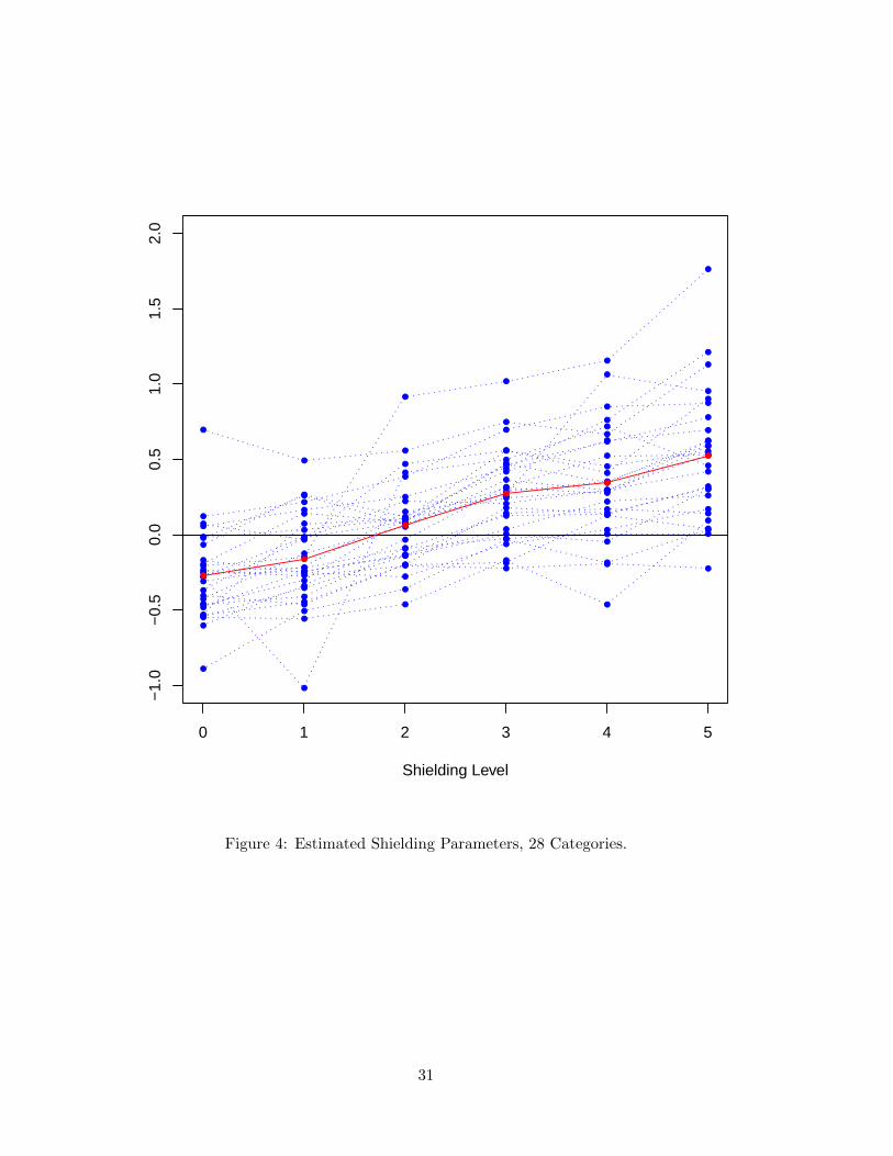
0 1 2 3 4 5

−1.

0−

0.5

0.0

0.5

1.0

1.5

2.0

Shielding Level

●

●●

●●

●

●

●

●

●

●●

●

●

●

●

●

●

● ●

●

●

●●

●●

● ●●

●

●

●

●

●

●

●

●

●

●

●

●

●

● ●

●

●● ●

●

●

●

●

●

●

●●

●

● ●

●

●

●●

●

●

●

●

●

●

●●

●

●

●

● ●

●

●

●

●

●

●

●

●

●

●

●

●

●

●

●

●

●

●

●

●

●

●

●

●

●

●

● ●

●

●

●

●

●●

●

●

●

●

●

●

● ●

●

●

●

●

●

●●

●

●

●

●

●

●

●

●

●

●

●●

●

●

●

●

●●

●

●

●

●

●

●

●

●

●

●

●

●

●

●

●

●

●

● ●

●

●

●

●

●

●

●

●

●

●

●

●

Figure 4: Estimated Shielding Parameters, 28 Categories.

31

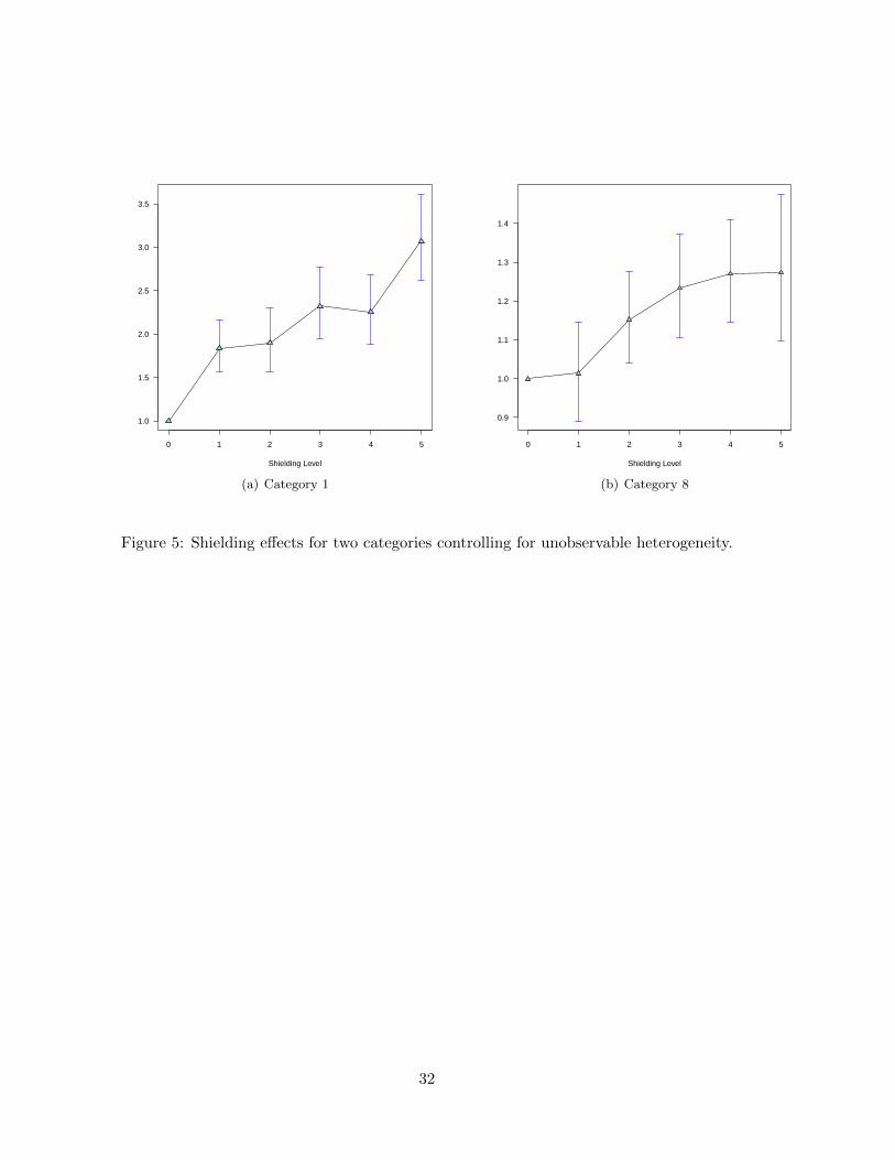
0 1 2 3 4 5

1.0

1.5

2.0

2.5

3.0

3.5

Shielding Level

(a) Category 1

0 1 2 3 4 5

0.9

1.0

1.1

1.2

1.3

1.4

Shielding Level

(b) Category 8

Figure 5: Shielding effects for two categories controlling for unobservable heterogeneity.

32

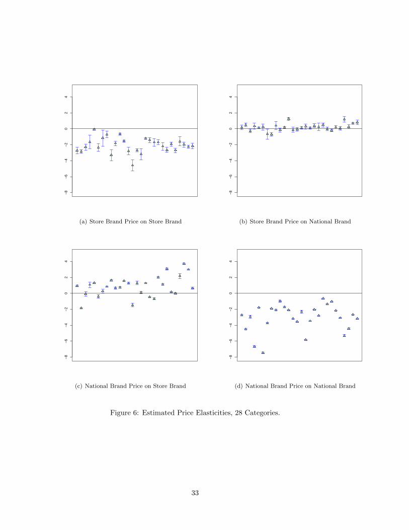
−8

−6

−4

−2

02

4

(a) Store Brand Price on Store Brand

−8

−6

−4

−2

02

4

(b) Store Brand Price on National Brand

−8

−6

−4

−2

02

4

(c) National Brand Price on Store Brand

−8

−6

−4

−2

02

4

(d) National Brand Price on National Brand

Figure 6: Estimated Price Elasticities, 28 Categories.

33

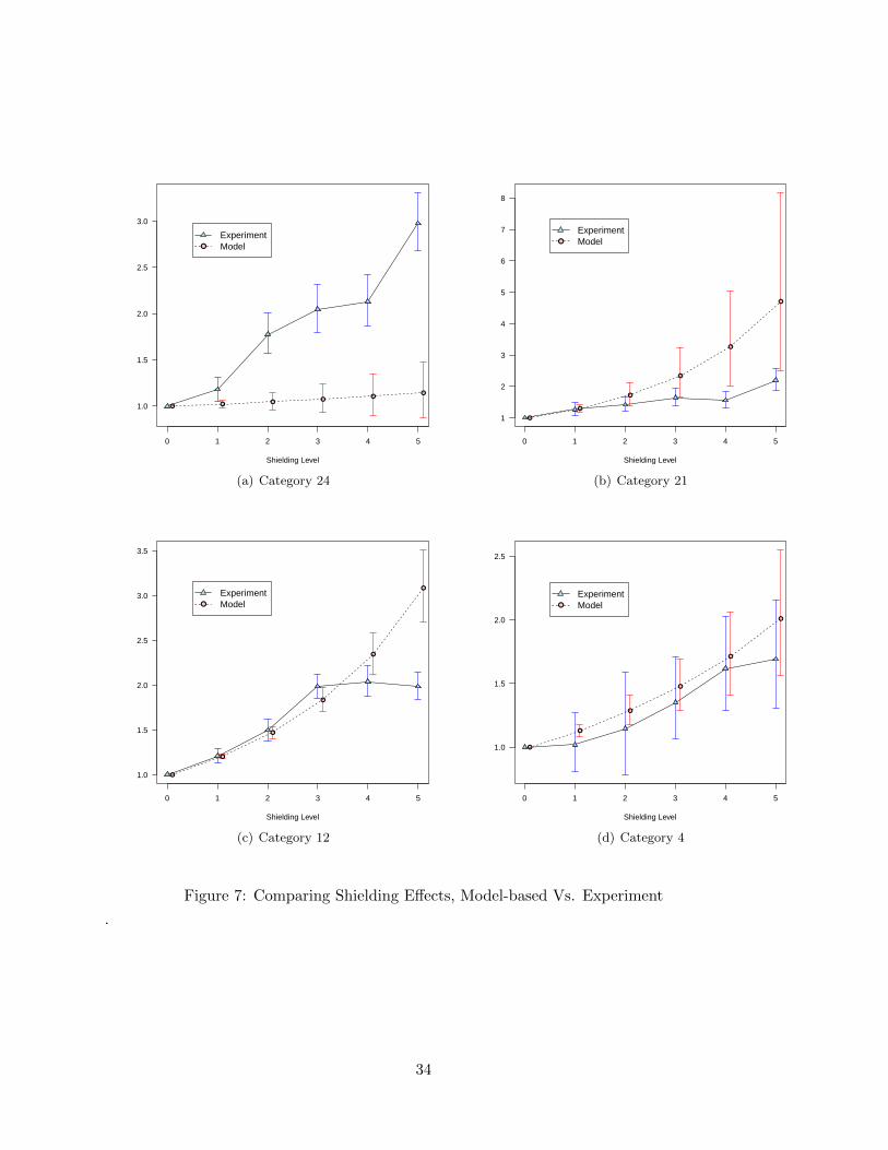
0 1 2 3 4 5

1.0

1.5

2.0

2.5

3.0

Shielding Level

● ● ●●

●●

●

ExperimentModel

(a) Category 24

0 1 2 3 4 5

1

2

3

4

5

6

7

8

Shielding Level

●

●

●

●

●

●

●

ExperimentModel

(b) Category 21

0 1 2 3 4 5

1.0

1.5

2.0

2.5

3.0

3.5

Shielding Level

●

●

●

●

●

●

●

ExperimentModel

(c) Category 12

0 1 2 3 4 5

1.0

1.5

2.0

2.5

Shielding Level

●

●

●

●

●

●

●

ExperimentModel

(d) Category 4

Figure 7: Comparing Shielding Effects, Model-based Vs. Experiment

.

34

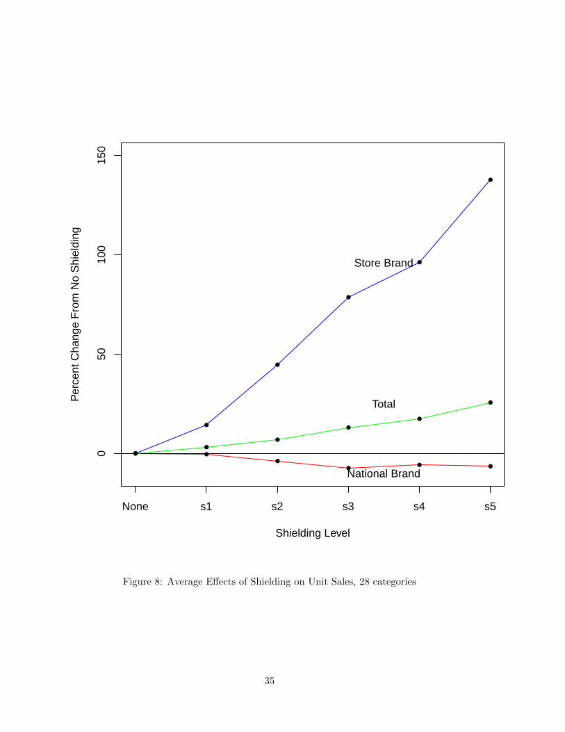
Shielding Level

Per

cent

Cha

nge

Fro

m N

o S

hiel

ding

050

100

150

None s1 s2 s3 s4 s5

●

●

●

●

●

●

●

●

●

●

●

●

● ●

●

●● ●

Store Brand

Total

National Brand

Figure 8: Average Effects of Shielding on Unit Sales, 28 categories

35

●

●

●

●

●

●

●

●

●

●

● ●

●

●

●

●

●

●

1000

020

000

3000

040

000

5000

060

000

Uni

t Sal

es

None s1 s2 s3 s4 s5Shielding Level

NB

SB

NB+SB

(a) Category 27

●

●

●

●●

●

●

●

●

●

●

●

●

●

●

●

●

●

2000

030

000

4000

050

000

Uni

t Sal

es

None s1 s2 s3 s4 s5Shielding Level

NB

SB

NB+SB

(b) Category 23

Figure 9: Average Effects of Shielding on Unit Sales, Two Categories.

36

●

●

●

●

●

●

●

●

●●

● ●

●

●

●

●

●

●

●

●

●

●

●

●

●

●

●

●

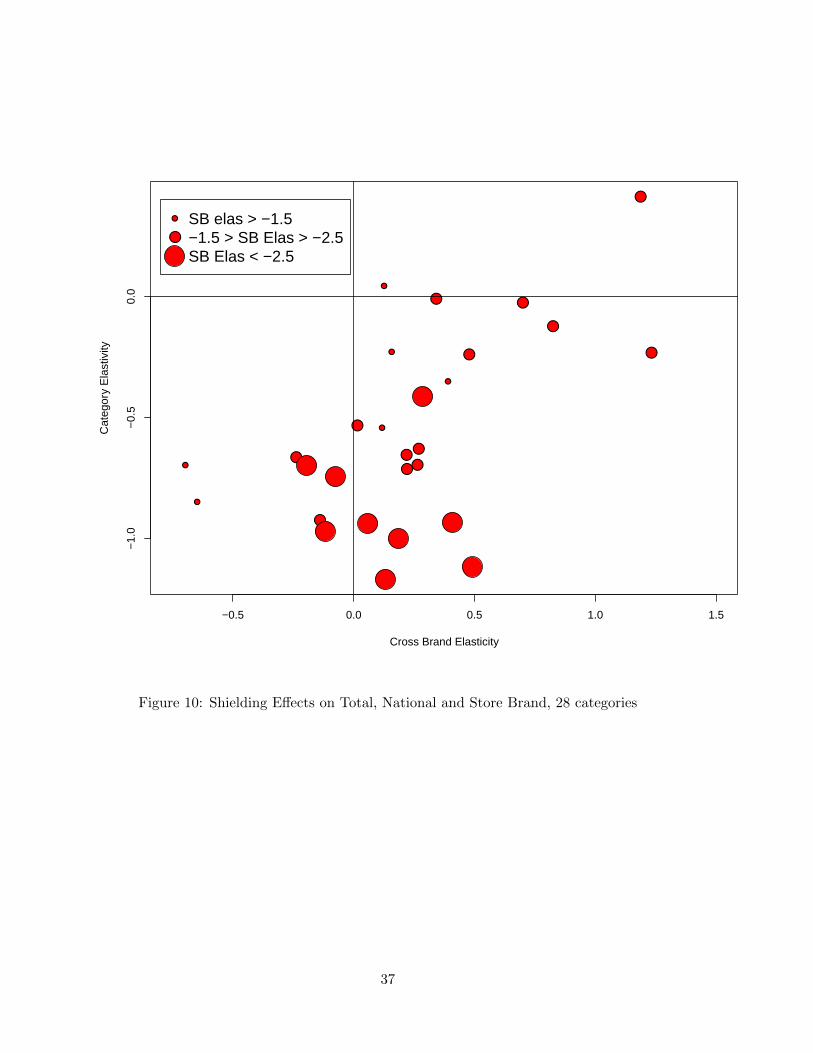
−0.5 0.0 0.5 1.0 1.5

−1.

0−

0.5

0.0

Cross Brand Elasticity

Cat

egor

y E

last

ivity

●

●●

●

●

●

●

● ●

●

●

●

●

●

●

●

●

●

●

●

●

SB elas > −1.5−1.5 > SB Elas > −2.5SB Elas < −2.5

Figure 10: Shielding Effects on Total, National and Store Brand, 28 categories

37

●

●

●

●

●

●

●●

●

●

●

●

●●

●

●

●

●

●

●

●

●

●

●

●

●

●

●

1.25 1.30 1.35 1.40 1.45

−0.

50.

00.

51.

0

Price_NB/Price_SB

Cro

ss P

rice

Ela

stic

ity

Correlation= −0.34

(a) Relative Price of National Brand and Cross Price Elas-

ticity

●

●

●

●

●

●

●●

●

●

●

●

●●

●

●

●

●

●

●

●

●

●

●

●

●

●

●

0.5 1.0 1.5 2.0

−0.

50.

00.

51.

0

SB Market Share/NB Market Share

Cro

ss P

rice

Ela

stic

ity

Correlation= 0.44

(b) Relative Store Brand Market Share and Cross Price

Elasticity

Figure 11: Explaining Cross Price Elasticities, 28 Categories.

38

●

●

●

●

●

●

●

●

●

●

●

●

●

●

●

●

●

●

●

●

●

●

●

●

●

●

●

●

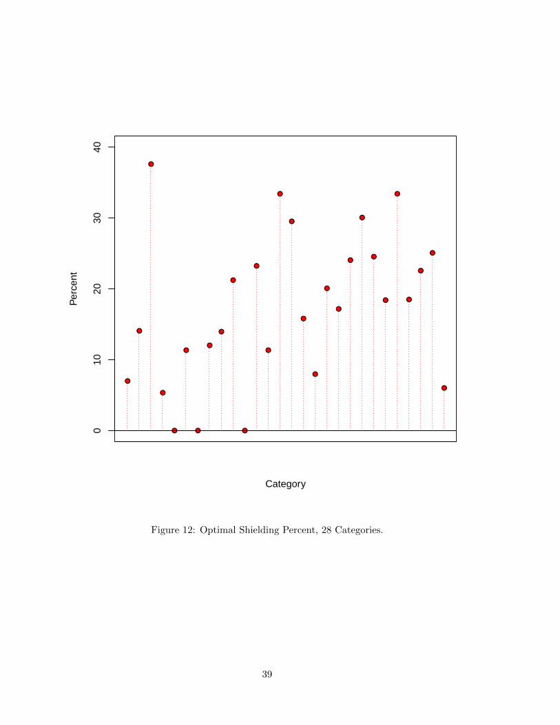
010

2030

40

Category

Per

cent

Figure 12: Optimal Shielding Percent, 28 Categories.

39

●

●

●

●

●

●

●

●

●

●

●

●

●

●

●

●

●

●

●

●

●

●

●

●

●

●

●

●

0 10 20 30 40

010

2030

40

NB Promotion Depth (Percent)

Opt

imal

Shi

eldi

ng P

erce

nt

Correlation= 0.12

(a) Optimal Shielding and Promotion Depth

●

●

●

●

●

●

●

●

●

●

●

●

●

●

●

●

●

●

●

●

●

●

●

●

●

●

●

●

−4 −3 −2 −1 0

010

2030

Store Brand Shielding Elasticity

Opt

imal

Shi

eldi

ng P

erce

nt

Correlation= −0.51

(b) Optimal Shielding and Store Brand Shielding Elasticity

Figure 13: Explaining Optimal Shielding.

0 1 2 3 4 5

6500

7000

7500

8000

8500

9000

9500

Shielding Level

Pro

fit

Profit (Experiment)Profit (Model)

(a) Category 13

0 1 2 3 4 5

8000

8500

9000

9500

Shielding Level

Pro

fit (

Exp

erim

ent)

1050

011

000

1150

012

000

Pro

fit (

Mod

el)

Profit (Experiment)Profit (Model)

(b) Category 3

Figure 14: Posterior Expected Profit for two categories.

40

0 5 10 15 20 25

Categories

Per

cent

5060

7080

9010

0

●

●

●

●

●●

●

●

●

●● ●

● ● ● ● ●●

● ● ●

●

●

●●

● ● ●

●

OptimalNo ActionDollar Gap MaintenancePercent Gap Maintenance

Figure 15: Evaluating Shielding Heuristics. Profit as a Percent of Profit from Optimal

Shielding.

41

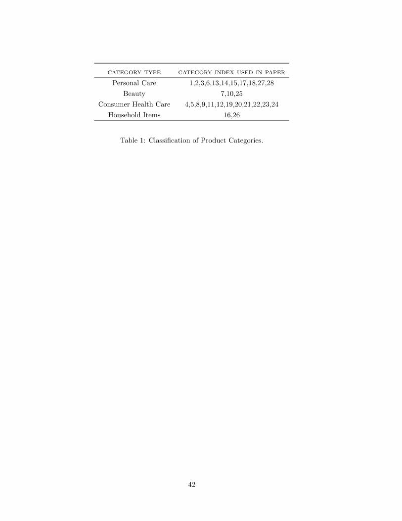
category type category index used in paper

Personal Care 1,2,3,6,13,14,15,17,18,27,28

Beauty 7,10,25

Consumer Health Care 4,5,8,9,11,12,19,20,21,22,23,24

Household Items 16,26

Table 1: Classification of Product Categories.

42

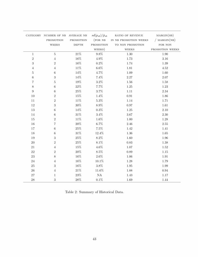
category number of nb average nb sd(psb)/p̄sb ratio of revenue margin(sb)

promotion promotion (for nb in nb promotion weeks / margin(nb)

weeks depth promotion to non promotion for non

weeks) weeks promotion weeks

1 5 21% 9.8% 1.30 1.90

2 4 16% 4.9% 1.73 3.16

3 2 16% 0.2% 1.74 1.39

4 4 11% 6.6% 1.81 4.52

5 6 14% 4.7% 1.09 1.60

6 3 14% 7.4% 2.27 2.07

7 5 19% 3.2% 1.56 1.58

8 6 22% 7.7% 1.25 1.23

9 6 25% 3.7% 1.11 2.34

10 2 15% 1.4% 0.91 1.86

11 2 11% 5.3% 1.14 1.71

12 3 30% 8.9% 0.97 1.61

13 6 14% 0.3% 1.25 2.10

14 6 31% 3.4% 3.67 2.30

15 2 11% 1.6% 1.00 1.28

16 7 20% 6.7% 2.46 2.55

17 6 25% 7.5% 1.42 1.41

18 6 31% 12.4% 1.36 1.65

19 3 25% 8.2% 1.60 1.96

20 2 25% 8.1% 0.83 1.38

21 4 15% 4.6% 1.07 1.52

22 2 20% 8.5% 0.89 1.15

23 8 16% 2.6% 1.06 1.91

24 4 16% 10.1% 1.28 1.79

25 3 16% 3.8% 1.95 1.99

26 4 21% 11.6% 1.88 0.94

27 1 23% NA 1.43 1.17

28 3 28% 0.1% 1.69 1.44

Table 2: Summary of Historical Data.

43

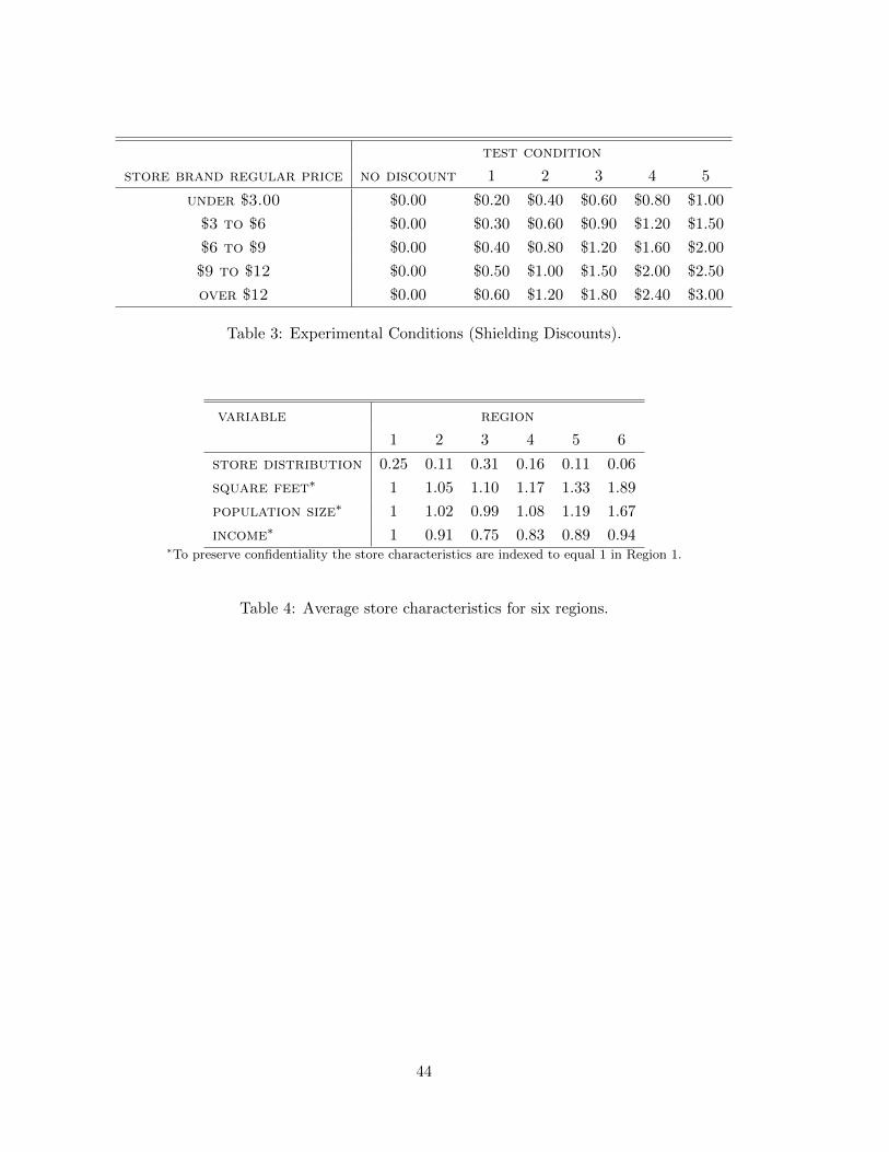
test condition

store brand regular price no discount 1 2 3 4 5

under $3.00 $0.00 $0.20 $0.40 $0.60 $0.80 $1.00

$3 to $6 $0.00 $0.30 $0.60 $0.90 $1.20 $1.50

$6 to $9 $0.00 $0.40 $0.80 $1.20 $1.60 $2.00

$9 to $12 $0.00 $0.50 $1.00 $1.50 $2.00 $2.50

over $12 $0.00 $0.60 $1.20 $1.80 $2.40 $3.00

Table 3: Experimental Conditions (Shielding Discounts).

variable region

1 2 3 4 5 6

store distribution 0.25 0.11 0.31 0.16 0.11 0.06

square feet∗ 1 1.05 1.10 1.17 1.33 1.89

population size∗ 1 1.02 0.99 1.08 1.19 1.67

income∗ 1 0.91 0.75 0.83 0.89 0.94∗To preserve confidentiality the store characteristics are indexed to equal 1 in Region 1.

Table 4: Average store characteristics for six regions.

44

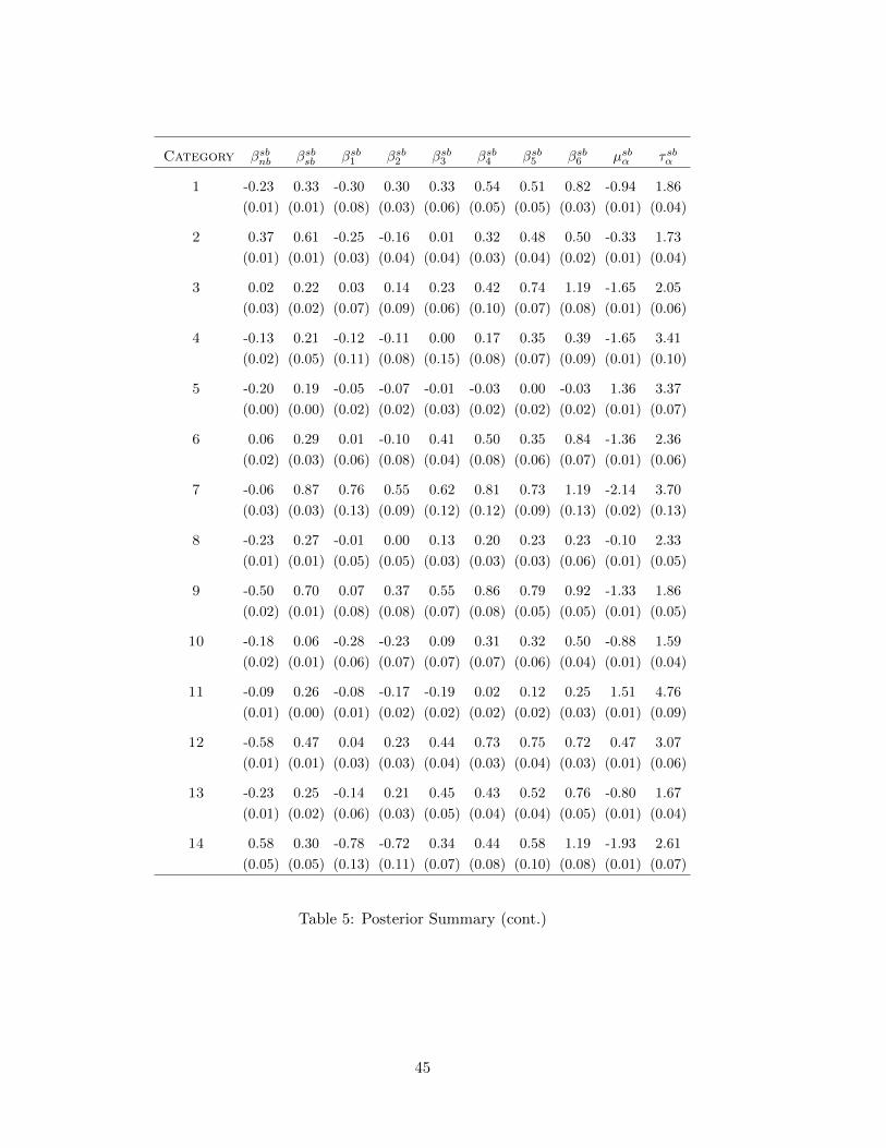
Category βsbnb βsbsb βsb1 βsb2 βsb3 βsb4 βsb5 βsb6 µsbα τsbα

1 -0.23 0.33 -0.30 0.30 0.33 0.54 0.51 0.82 -0.94 1.86

(0.01) (0.01) (0.08) (0.03) (0.06) (0.05) (0.05) (0.03) (0.01) (0.04)

2 0.37 0.61 -0.25 -0.16 0.01 0.32 0.48 0.50 -0.33 1.73

(0.01) (0.01) (0.03) (0.04) (0.04) (0.03) (0.04) (0.02) (0.01) (0.04)

3 0.02 0.22 0.03 0.14 0.23 0.42 0.74 1.19 -1.65 2.05

(0.03) (0.02) (0.07) (0.09) (0.06) (0.10) (0.07) (0.08) (0.01) (0.06)

4 -0.13 0.21 -0.12 -0.11 0.00 0.17 0.35 0.39 -1.65 3.41

(0.02) (0.05) (0.11) (0.08) (0.15) (0.08) (0.07) (0.09) (0.01) (0.10)

5 -0.20 0.19 -0.05 -0.07 -0.01 -0.03 0.00 -0.03 1.36 3.37

(0.00) (0.00) (0.02) (0.02) (0.03) (0.02) (0.02) (0.02) (0.01) (0.07)

6 0.06 0.29 0.01 -0.10 0.41 0.50 0.35 0.84 -1.36 2.36

(0.02) (0.03) (0.06) (0.08) (0.04) (0.08) (0.06) (0.07) (0.01) (0.06)

7 -0.06 0.87 0.76 0.55 0.62 0.81 0.73 1.19 -2.14 3.70

(0.03) (0.03) (0.13) (0.09) (0.12) (0.12) (0.09) (0.13) (0.02) (0.13)

8 -0.23 0.27 -0.01 0.00 0.13 0.20 0.23 0.23 -0.10 2.33

(0.01) (0.01) (0.05) (0.05) (0.03) (0.03) (0.03) (0.06) (0.01) (0.05)

9 -0.50 0.70 0.07 0.37 0.55 0.86 0.79 0.92 -1.33 1.86

(0.02) (0.01) (0.08) (0.08) (0.07) (0.08) (0.05) (0.05) (0.01) (0.05)

10 -0.18 0.06 -0.28 -0.23 0.09 0.31 0.32 0.50 -0.88 1.59

(0.02) (0.01) (0.06) (0.07) (0.07) (0.07) (0.06) (0.04) (0.01) (0.04)

11 -0.09 0.26 -0.08 -0.17 -0.19 0.02 0.12 0.25 1.51 4.76

(0.01) (0.00) (0.01) (0.02) (0.02) (0.02) (0.02) (0.03) (0.01) (0.09)

12 -0.58 0.47 0.04 0.23 0.44 0.73 0.75 0.72 0.47 3.07

(0.01) (0.01) (0.03) (0.03) (0.04) (0.03) (0.04) (0.03) (0.01) (0.06)

13 -0.23 0.25 -0.14 0.21 0.45 0.43 0.52 0.76 -0.80 1.67

(0.01) (0.02) (0.06) (0.03) (0.05) (0.04) (0.04) (0.05) (0.01) (0.04)

14 0.58 0.30 -0.78 -0.72 0.34 0.44 0.58 1.19 -1.93 2.61

(0.05) (0.05) (0.13) (0.11) (0.07) (0.08) (0.10) (0.08) (0.01) (0.07)

Table 5: Posterior Summary (cont.)

45

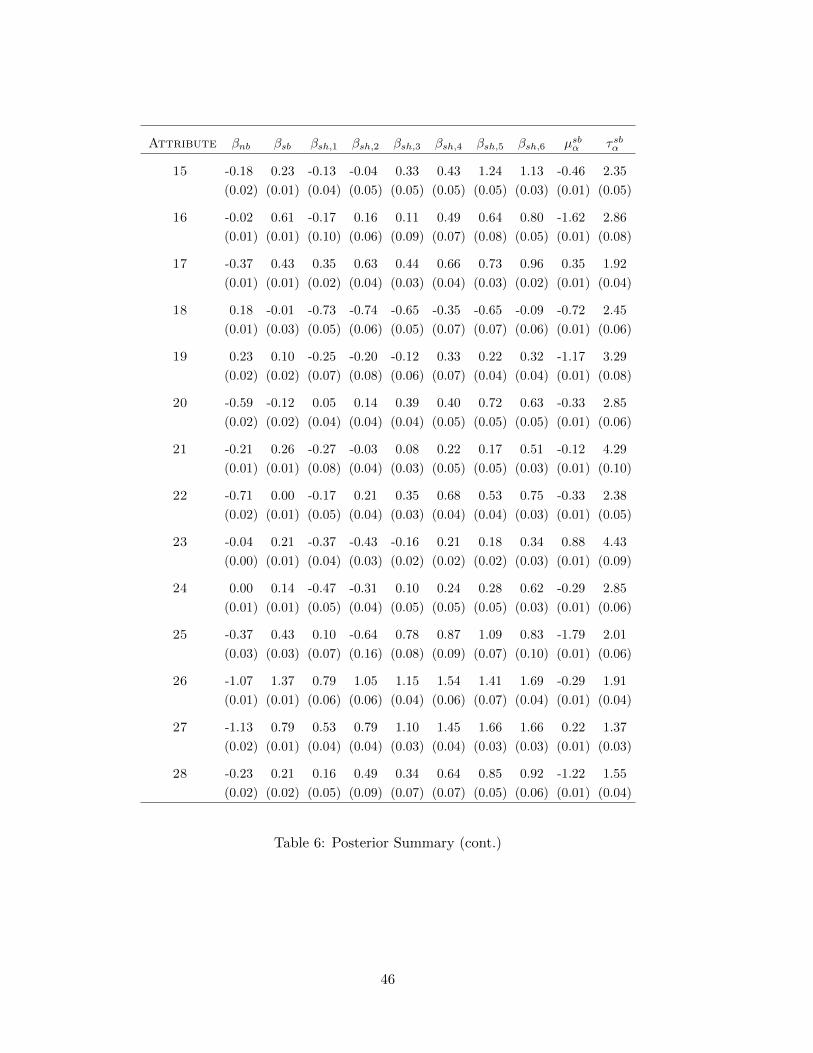
Attribute βnb βsb βsh,1 βsh,2 βsh,3 βsh,4 βsh,5 βsh,6 µsbα τsbα

15 -0.18 0.23 -0.13 -0.04 0.33 0.43 1.24 1.13 -0.46 2.35

(0.02) (0.01) (0.04) (0.05) (0.05) (0.05) (0.05) (0.03) (0.01) (0.05)

16 -0.02 0.61 -0.17 0.16 0.11 0.49 0.64 0.80 -1.62 2.86

(0.01) (0.01) (0.10) (0.06) (0.09) (0.07) (0.08) (0.05) (0.01) (0.08)

17 -0.37 0.43 0.35 0.63 0.44 0.66 0.73 0.96 0.35 1.92

(0.01) (0.01) (0.02) (0.04) (0.03) (0.04) (0.03) (0.02) (0.01) (0.04)

18 0.18 -0.01 -0.73 -0.74 -0.65 -0.35 -0.65 -0.09 -0.72 2.45

(0.01) (0.03) (0.05) (0.06) (0.05) (0.07) (0.07) (0.06) (0.01) (0.06)

19 0.23 0.10 -0.25 -0.20 -0.12 0.33 0.22 0.32 -1.17 3.29

(0.02) (0.02) (0.07) (0.08) (0.06) (0.07) (0.04) (0.04) (0.01) (0.08)

20 -0.59 -0.12 0.05 0.14 0.39 0.40 0.72 0.63 -0.33 2.85

(0.02) (0.02) (0.04) (0.04) (0.04) (0.05) (0.05) (0.05) (0.01) (0.06)

21 -0.21 0.26 -0.27 -0.03 0.08 0.22 0.17 0.51 -0.12 4.29

(0.01) (0.01) (0.08) (0.04) (0.03) (0.05) (0.05) (0.03) (0.01) (0.10)

22 -0.71 0.00 -0.17 0.21 0.35 0.68 0.53 0.75 -0.33 2.38

(0.02) (0.01) (0.05) (0.04) (0.03) (0.04) (0.04) (0.03) (0.01) (0.05)

23 -0.04 0.21 -0.37 -0.43 -0.16 0.21 0.18 0.34 0.88 4.43

(0.00) (0.01) (0.04) (0.03) (0.02) (0.02) (0.02) (0.03) (0.01) (0.09)

24 0.00 0.14 -0.47 -0.31 0.10 0.24 0.28 0.62 -0.29 2.85

(0.01) (0.01) (0.05) (0.04) (0.05) (0.05) (0.05) (0.03) (0.01) (0.06)

25 -0.37 0.43 0.10 -0.64 0.78 0.87 1.09 0.83 -1.79 2.01

(0.03) (0.03) (0.07) (0.16) (0.08) (0.09) (0.07) (0.10) (0.01) (0.06)

26 -1.07 1.37 0.79 1.05 1.15 1.54 1.41 1.69 -0.29 1.91

(0.01) (0.01) (0.06) (0.06) (0.04) (0.06) (0.07) (0.04) (0.01) (0.04)

27 -1.13 0.79 0.53 0.79 1.10 1.45 1.66 1.66 0.22 1.37

(0.02) (0.01) (0.04) (0.04) (0.03) (0.04) (0.03) (0.03) (0.01) (0.03)

28 -0.23 0.21 0.16 0.49 0.34 0.64 0.85 0.92 -1.22 1.55

(0.02) (0.02) (0.05) (0.09) (0.07) (0.07) (0.05) (0.06) (0.01) (0.04)

Table 6: Posterior Summary (cont.)

46

profit increase

action mean sd min max

optimal shielding 21.6% 19.5% 0.0% 86.9%

dollar gap maintenance 7.9% 22.8% -33.8% 86.9%

percent gap maintenance 6.1% 19.4% -22.7% 86.9%

Table 7: Profit Increase Compared to No Shielding. Summary for 28 Categories.

47