Sheet Pile Wall
27
COMPUTATIONAL GEOMECHANICS Arnold Verruijt Kluwer Academic Publishers Dordrecht/Boston/London 1995 ISBN 0-7923-3407-8
-
Upload
giovanni-govdon-bugli -
Category
Documents
-
view
98 -
download
0
Transcript of Sheet Pile Wall
COMPUTATIONALGEOMECHANICS
Arnold Verruijt
Kluwer Academic Publishers
Dordrecht/Boston/London
1995
ISBN 0-7923-3407-8

CONTENTS
1 Soil Properties . . . . . . . . . . . . . . . . . . . . . . . . . . . . . . . . . . . . . . . . . . . . . . . . . . . . . . . . . . . . 1
2 Theory of Consolidation . . . . . . . . . . . . . . . . . . . . . . . . . . . . . . . . . . . . . . . . . . . . . . . . . . . 8
3 Sea Bed Response to Cyclic Loads . . . . . . . . . . . . . . . . . . . . . . . . . . . . . . . . . . . . . . . . 35
4 Beams on Elastic Foundation . . . . . . . . . . . . . . . . . . . . . . . . . . . . . . . . . . . . . . . . . . . . . 53
5 Sheet Pile Walls . . . . . . . . . . . . . . . . . . . . . . . . . . . . . . . . . . . . . . . . . . . . . . . . . . . . . . . . . . 67
6 Axially Loaded Piles . . . . . . . . . . . . . . . . . . . . . . . . . . . . . . . . . . . . . . . . . . . . . . . . . . . . . 78
7 Development of Pile Plug . . . . . . . . . . . . . . . . . . . . . . . . . . . . . . . . . . . . . . . . . . . . . . . 106
8 Laterally Loaded Piles . . . . . . . . . . . . . . . . . . . . . . . . . . . . . . . . . . . . . . . . . . . . . . . . . . 122
9 Pile in Layered Elastic Material . . . . . . . . . . . . . . . . . . . . . . . . . . . . . . . . . . . . . . . . . 151
10 Waves in Piles . . . . . . . . . . . . . . . . . . . . . . . . . . . . . . . . . . . . . . . . . . . . . . . . . . . . . . . . . . 167
11 Gravity Foundations . . . . . . . . . . . . . . . . . . . . . . . . . . . . . . . . . . . . . . . . . . . . . . . . . . . . 194
12 Slope Stability . . . . . . . . . . . . . . . . . . . . . . . . . . . . . . . . . . . . . . . . . . . . . . . . . . . . . . . . . . 204
13 Finite Elements for Plane Groundwater Flow . . . . . . . . . . . . . . . . . . . . . . . . . . . . 219
14 Finite Elements for Plane Strain Elastostatics . . . . . . . . . . . . . . . . . . . . . . . . . . . . ??
15 Finite Elements for Plane Strain Elasto-plasticity . . . . . . . . . . . . . . . . . . . . . . . . 266
16 Finite Elements for One-dimensional Consolidation . . . . . . . . . . . . . . . . . . . . . . 280
17 Finite Elements for Two-dimensional Consolidation . . . . . . . . . . . . . . . . . . . . . . 291
18 Transport in Porous Media . . . . . . . . . . . . . . . . . . . . . . . . . . . . . . . . . . . . . . . . . . . . . . 308
19 Adsorption and Dispersion . . . . . . . . . . . . . . . . . . . . . . . . . . . . . . . . . . . . . . . . . . . . . . 337
Appendix A. Integral Transforms . . . . . . . . . . . . . . . . . . . . . . . . . . . . . . . . . . . . . . . . . 356
Appendix B. Solution of Linear Equations . . . . . . . . . . . . . . . . . . . . . . . . . . . . . . . . 365
References . . . . . . . . . . . . . . . . . . . . . . . . . . . . . . . . . . . . . . . . . . . . . . . . . . . . . . . . . . . . . . . . 375
Index . . . . . . . . . . . . . . . . . . . . . . . . . . . . . . . . . . . . . . . . . . . . . . . . . . . . . . . . . . . . . . . . . . . . . . 380
1
Chapter 4
BEAMS ON ELASTIC FOUNDATION
In this chapter a numerical method for the solution of the problem of a beam on anelastic foundation is presented. Special care will be taken that the program can beused for beams consisting of sections of unequal length, as the program is to be usedas a basis for a sheet pile wall program, and for a program for a laterally loaded pilein a layered soil.
4.1 Beam theory
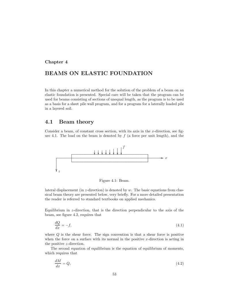
Consider a beam, of constant cross section, with its axis in the x-direction, see fig-ure 4.1. The load on the beam is denoted by f (a force per unit length), and the
.....................................................................................................................................................................................................................................................................................................................................................................................................................................................................................................................
.....................................................................................................................................................................................................................................................................................................................................................................................................................................................................................................................
........
........
........
........
........
........
...
........
........
........
........
........
........
...
............................................................................................................................................................................................................................................................................................................................................................................................................................................................................................................................................................................................................................................................................................................................................. ................................................................................................................
........................
................................................
................................................
................................................
..................................................
.....................................................
..........................................................
...............................................................
....................................................................
x
z
f
Figure 4.1: Beam.
lateral displacement (in z-direction) is denoted by w. The basic equations from clas-sical beam theory are presented below, very briefly. For a more detailed presentationthe reader is referred to standard textbooks on applied mechanics.
Equilibrium in z-direction, that is the direction perpendicular to the axis of thebeam, see figure 4.2, requires that
dQ
dx= −f, (4.1)
where Q is the shear force. The sign convention is that a shear force is positivewhen the force on a surface with its normal in the positive x-direction is acting inthe positive z-direction.
The second equation of equilibrium is the equation of equilibrium of moments,which requires that
dM
dx= Q, (4.2)
53

54 4. BEAMS ON ELASTIC FOUNDATION
........
........
........
........
........
........
........
........
........
........
........
........
........
........
........
........
........
........
........
........
........
........
........
........
........
..................................................................................................................................................................................................................................................................................................................................................................................................................... . . . . . . . . . .. . . . . . . . . .. . . . . . . . . . .. . . . . . . . . .. . . . . . . . . . .. . . . . . . . . .. . . . . . . . . . .. . . . . . . . . .. . . . . . . . . . .. . . . . . . . . .. . . . . . . . . . .. . . . . . . . . .. . . . . . . . . . .. . . . . . . . . .. . . . . . . . . . .. . . . . . . . . .. . . . . . . . . . .. . . . . . . . . .. . . . . . . . . . .. . . . . . . . . .. . . . . . . . . . .. . . . . . . . . .. . . . . . . . . . .. . . . . . . . . .. . . . . . . . . . .. . . . . . . . . .. . . . . . . . . . .. . . . . . . . . .. . . . . . . . . . .. . . . . . . . . .. . . . . . . . . . .. . . . . . . . . .. . . . . . . . . . .. . . . . . . . . .. . . . . . . . . . .. . . . . . . . . .. . . . . . . . . . .. . . . . . . . . .. . . . . . . . . . .. . . . . . . . . .. . . . . . . . . . .
..................................................................................................................................................................................................................................................................................................................................................................................................................................................................................................................................... .......................................................................................................................................................................................................
........
........
........
........
........
........
........
........
........
........
........
........
........
........
........
........
........
........
.......................
................
.................................................................................................................................................................................................
.........................................................................
.........................................................................
.........................................................................
.........................................................................
..................
........................................................................................................................
..................................................................................................................................
...............
............................................... ...........
....................................
..................................................................................................................... ................ .....................................................................................................................................
..............................
..............................
x
z
f
Q
Q + ∆Q
M M + ∆M
∆x
Figure 4.2: Element of beam.
where M is the bending moment. The sign convention is that a positive bendingmoment corresponds to a positive stress (tension) on the positive side of the axis ofthe beam.
The two equations of equilibrium can be combined to give
d2M
dx2= −f. (4.3)
This is the first basic equation of the theory of bending of beams.The second basic equation can be derived from a consideration of the deforma-
tions of the beam. When it is assumed that plane cross sections of the beam remainplane after deformation (Bernoulli’s hypothesis), and that the rotation dw/dx issmall compared to 1, one obtains
EId2w
dx2= −M, (4.4)
where EI is the flexural rigidity of the beam.The two basic equations (4.3) and (4.4) can be combined to give
EId4w
dx4= f. (4.5)
This is a fourth order differential equation for the lateral displacement, the basicequation of the classical theory of bending of beams.
Equation (4.5) can be solved analytically or numerically, subject to the appro-priate boundary conditions.
4.2 Beam on elastic foundation
For a beam on an elastic foundation the lateral load consists of the external load,and a soil reaction. As a first approximation the soil reaction is assumed to be

4.2. Beam on elastic foundation 55
.....................................................................................................................................................................................................................................................................................................................................................................................................................................................................................................................
.....................................................................................................................................................................................................................................................................................................................................................................................................................................................................................................................
........
........
........
........
........
........
...
........
........
........
........
........
........
...
............................................................................................................................................................................................................................................................................................................................................................................................................................................................................................................................................................................................................................................................................................................................................. ................................................................................................................
........................
. . . . . . . . . . . . . . . . . . . . . . . . . . . . . . . . . . . . . . . . . . . . . . . . . . . . . . . . . . . . .. . . . . . . . . . . . . . . . . . . . . . . . . . . . . . . . . . . . . . . . . . . . . . . . . . . . . . . . . . . .. . . . . . . . . . . . . . . . . . . . . . . . . . . . . . . . . . . . . . . . . . . . . . . . . . . . . . . . . . . . .. . . . . . . . . . . . . . . . . . . . . . . . . . . . . . . . . . . . . . . . . . . . . . . . . . . . . . . . . . . .. . . . . . . . . . . . . . . . . . . . . . . . . . . . . . . . . . . . . . . . . . . . . . . . . . . . . . . . . . . . .. . . . . . . . . . . . . . . . . . . . . . . . . . . . . . . . . . . . . . . . . . . . . . . . . . . . . . . . . . . .
................................................
................................................
................................................
..................................................
.....................................................
..........................................................
...............................................................
....................................................................
x
z
f
Figure 4.3: Beam on elastic foundation.
proportional to the lateral displacement. The basic differential equation now is
EId4w
dx4= f − kw, (4.6)
where k is the subgrade modulus.Various analytical solutions of this differential equation have been obtained, see
Hetenyi (1946). The homogeneous equation, obtained if f = 0, has solutions of theform
w = C1 exp(x/λ) sin(x/λ) + C2 exp(x/λ) cos(x/λ) +C3 exp(−x/λ) sin(x/λ) + C4 exp(−x/λ) cos(x/λ), (4.7)
where λ4 = 4 EI/k. These solutions play an important role in the theory. It shouldbe noted that a characteristic wave length of the solutions is 2πλ. In a numericalsolution it is advisable to take care that the interval length is small compared tothis wave length.
In this chapter a numerical solution method will be presented. In solving the dif-ferential equation (4.6) by a numerical method it has to be noted that the bendingmoment M is obtained as the second derivative of the variable w, and the shear forceQ as the third derivative. This means that, if the problem is solved as a problemin the variable w only, much accuracy will be lost when passing to the bending mo-ment and the shear force. As these are important engineering quantities some othertechnique may be more appropriate. For this purpose it is convenient to return tothe basic equations as they were derived in the previous section. Thus the basicequations are considered to be
d2M
dx2= −f + kw. (4.8)
and
EId2w
dx2= −M. (4.9)
Although this system of two second order differential equations is of course com-pletely equivalent to the single fourth order equation (4.6), in a numerical approachit may be more accurate to set up the method in terms of the two variables w andM . This will be elaborated in the next section.
56 4. BEAMS ON ELASTIC FOUNDATION
4.3 Numerical model
In order to derive the equations describing the numerical model, special attentionwill be paid to the physical background of the equations. In this respect it is con-sidered more important, for instance, that the equilibrium equations are satisfied asaccurately as possible, rather than to use a strictly mathematical elaboration of thedifferential equations.
4.3.1 Basic equations
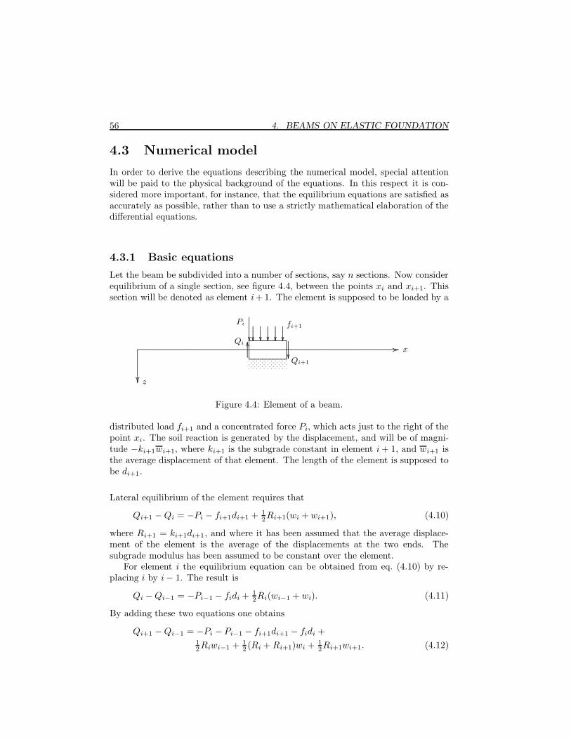
Let the beam be subdivided into a number of sections, say n sections. Now considerequilibrium of a single section, see figure 4.4, between the points xi and xi+1. Thissection will be denoted as element i + 1. The element is supposed to be loaded by a
.....................................................................................................
.....................................................................................................
........
........
........
........
........
........
...
........
........
........
........
........
........
...
............................................................................................................................................................................................................................................................................................................................................................................................................................................................................................................................................................................................................................................................................................................................................. ................................................................................................................
........................
. . . . . . . . . . .. . . . . . . . . .. . . . . . . . . . .. . . . . . . . . .. . . . . . . . . . .. . . . . . . . . .
............................................................
............................................................
............................................................
............................................................
............................................................
........
........
........
........
........
............
...............................................................................
.....................................................................................
x
z
fi+1
Qi
Qi+1
Pi
Figure 4.4: Element of a beam.
distributed load fi+1 and a concentrated force Pi, which acts just to the right of thepoint xi. The soil reaction is generated by the displacement, and will be of magni-tude −ki+1wi+1, where ki+1 is the subgrade constant in element i + 1, and wi+1 isthe average displacement of that element. The length of the element is supposed tobe di+1.
Lateral equilibrium of the element requires that
Qi+1 − Qi = −Pi − fi+1di+1 + 12Ri+1(wi + wi+1), (4.10)
where Ri+1 = ki+1di+1, and where it has been assumed that the average displace-ment of the element is the average of the displacements at the two ends. Thesubgrade modulus has been assumed to be constant over the element.
For element i the equilibrium equation can be obtained from eq. (4.10) by re-placing i by i − 1. The result is
Qi − Qi−1 = −Pi−1 − fidi + 12Ri(wi−1 + wi). (4.11)
By adding these two equations one obtains
Qi+1 − Qi−1 = −Pi − Pi−1 − fi+1di+1 − fidi +12Riwi−1 + 1
2 (Ri + Ri+1)wi + 12Ri+1wi+1. (4.12)

4.3. Numerical model 57
This can, of course, also be considered as the equation of equilibrium of the twoelements i and i + 1 together.
Equilibrium of moments of element i + 1 about its center requires that
Mi+1 − Mi = 12 (Qi+1 + Qi)di+1 − 1
2Pidi+1. (4.13)
Replacing i by i − 1 gives the equation of moment equilibrium for element i,
Mi − Mi−1 = 12 (Qi + Qi−1)di − 1
2Pi−1di. (4.14)
Elimination of Qi from (4.13) and (4.14) gives
1di+1
Mi+1 − (1
di+1+
1di
)Mi +1di
Mi−1 =
12 (Qi+1 − Qi−1 − Pi + Pi−1), (4.15)
or, with (4.12),
1di+1
Mi+1 − (1
di+1+
1di
)Mi +1di
Mi−1
−14Ri+1wi+1 − 1
4(Ri + Ri+1)wi − 14Riwi−1 =
−12(difi + di+1fi+1) − Pi. (4.16)
This is the first basic equation of the numerical model. It is the numerical equiv-alent of eq. (4.8). All terms can easily be recognized, but the precise value of allthe coefficients is not immediately clear. For this purpose the complete derivationpresented above has to be processed.
The second basic equation must be the numerical equivalent of equation (4.9). Thiscan be obtained as follows. Consider the two elements to the left and to the rightof point xi. In the element to the left (element i) we have
x < xi : EId2w
dx2= −1
2(Mi−1 + Mi), (4.17)
where it has been assumed that the bending moment in this element is the averageof the values at the two ends. On the other hand we have in element i + 1,
x > xi : EId2w
dx2= −1
2(Mi + Mi+1). (4.18)
These two equations can be integrated, assuming that the right hand side is constant,to give
x < xi : EIw = −14(Mi−1 + Mi)(x − xi)2 +
A(x − xi) + EIwi, (4.19)

58 4. BEAMS ON ELASTIC FOUNDATION
and
x > xi : EIw = −14(Mi + Mi+1)(x − xi)2 +
A(x − xi) + EIwi, (4.20)
where the integration constants have been chosen such that for x = xi the displace-ment is always wi and the slope is continuous at that point (namely A/EI).
Substituting x = xi−1 in eq. (4.19) and x = xi+1 into eq. (4.20) gives two expressionsfor A. After elimination of A one obtains, finally,
EI
di+1wi+1 − (
EI
di+1+
EI
di)wi +
EI
diwi−1
+14di+1Mi+1 + 1
4(di+1 + di)Mi + 1
4diMi−1 = 0. (4.21)
This is the second basic equation of the numerical model, the numerical equivalentof the differential equation (4.9). Its form is very similar to the first basic equation,eq. (4.16). When all the elements have the same size d, and all the coefficients in thesecond part of the equation are lumped together, a simplified form of this equationis
EI
d2wi+1 −
2EI
d2wi +
EI
d2wi−1 + Mi = 0. (4.22)
This is a well known approximation of eq. (4.4) by central finite differences. Therefinements in eq. (4.21) are due to the use of unequal intervals and a more refinedapproximation of the bending moment.
4.3.2 Boundary conditions
The boundary conditions must also be expressed numerically. This requires somecareful consideration, as it is most convenient if the two boundary conditions ateither end of the beam can be expressed in terms of w and M in these points. Thisis very simple in the case of a hinged support (then w = 0 and M = 0). For otherboundary conditions, such as a clamped boundary or a free boundary, the boundaryconditions must be somewhat manipulated in order for them to be expressed in thetwo basic variables. If the left end of the beam is free the boundary conditions are
M0 = −M`, (4.23)
Q0 = −F`, (4.24)
where M` is a given external moment, and F` is a given force. The first boundarycondition can immediately be incorporated into the system of equations, but thesecond condition needs some special attention, because the shear force has beeneliminated from the system of equations. In this case equation (4.10) gives, withi = 0,
Q1 = −F` − f1d1 + 12R1(w0 + w1). (4.25)

4.3. Numerical model 59
This equation expresses lateral equilibrium of the first element. On the other hand,the equation of equilibrium of moments of the first element gives, with (4.13) fori = 0,
M1 − M0 = 12(Q1 − F`)d1. (4.26)
Elimination of Q1 from these two equations gives
12R1w0 + 1
2R1w1 +2d1
M0 − 2d1
M1 = f1d1 + 2F`. (4.27)
In this form the boundary condition (4.24) can be incorporated into the systemof algebraic equations. It gives a relation between the bending moments and thedisplacements in the first two points.
If the left end of the beam is fully clamped the boundary conditions are
w0 = 0, (4.28)
x = 0 :∂w
∂x= 0. (4.29)
The first condition can immediately be incorporated into the system of equations.The second condition can best be taken into account by considering equation (4.22)for i = 0,
EI
d2w1 −
2EI
d2w0 +
EI
d2w−1 + M0 = 0. (4.30)
The boundary condition (4.29) can be assumed to be satisfied by the symmetrycondition w−1 = w1, and thus, because w0 = 0,
2EI
d2w1 + M0 = 0. (4.31)
The distance d in this equation must be interpreted as the length of the first ele-ment. The condition (4.31) can easily be incorporated into the system of algebraicequations.
The boundary conditions at the right end of the beam can be taken into accountin a similar way as those at the left end.
4.3.3 Computer program
An elementary computer program, in Turbo Pascal, is reproduced below, as theprogram WINKLER. The program applies to a beam consisting of a number ofsections. Each section can have a different load, and have a different subgradeconstant. In the points separating two sections concentrated loads can be applied.The two boundaries can be clamped, hinged or free. Output is given in the form ofa list on the screen.
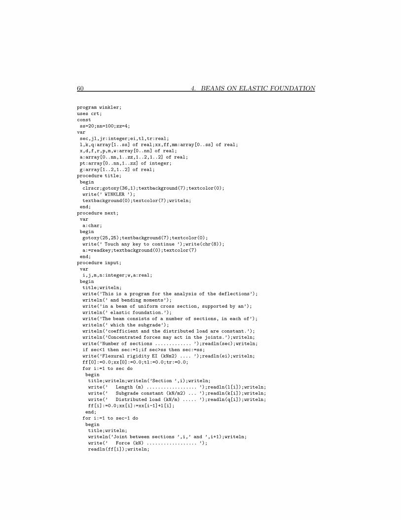
60 4. BEAMS ON ELASTIC FOUNDATION
program winkler;
uses crt;
const
ss=20;nn=100;zz=4;
var
sec,jl,jr:integer;ei,tl,tr:real;
l,k,q:array[1..ss] of real;xx,ff,mm:array[0..ss] of real;
x,d,f,r,p,m,w:array[0..nn] of real;
a:array[0..nn,1..zz,1..2,1..2] of real;
pt:array[0..nn,1..zz] of integer;
g:array[1..2,1..2] of real;
procedure title;
begin
clrscr;gotoxy(36,1);textbackground(7);textcolor(0);
write(’ WINKLER ’);
textbackground(0);textcolor(7);writeln;
end;
procedure next;
var
a:char;
begin
gotoxy(25,25);textbackground(7);textcolor(0);
write(’ Touch any key to continue ’);write(chr(8));
a:=readkey;textbackground(0);textcolor(7)
end;
procedure input;
var
i,j,m,n:integer;w,a:real;
begin
title;writeln;
write(’This is a program for the analysis of the deflections’);
writeln(’ and bending moments’);
write(’in a beam of uniform cross section, supported by an’);
writeln(’ elastic foundation.’);
write(’The beam consists of a number of sections, in each of’);
writeln(’ which the subgrade’);
writeln(’coefficient and the distributed load are constant.’);
writeln(’Concentrated forces may act in the joints.’);writeln;
write(’Number of sections ............. ’);readln(sec);writeln;
if sec<1 then sec:=1;if sec>ss then sec:=ss;
write(’Flexural rigidity EI (kNm2) .... ’);readln(ei);writeln;
ff[0]:=0.0;xx[0]:=0.0;tl:=0.0;tr:=0.0;
for i:=1 to sec do
begin
title;writeln;writeln(’Section ’,i);writeln;
write(’ Length (m) .................. ’);readln(l[i]);writeln;
write(’ Subgrade constant (kN/m2) ... ’);readln(k[i]);writeln;
write(’ Distributed load (kN/m) ..... ’);readln(q[i]);writeln;
ff[i]:=0.0;xx[i]:=xx[i-1]+l[i];
end;
for i:=1 to sec-1 do
begin
title;writeln;
writeln(’Joint between sections ’,i,’ and ’,i+1);writeln;
write(’ Force (kN) .................. ’);
readln(ff[i]);writeln;

4.3. Numerical model 61
end;
title;writeln;
writeln(’Boundary condition at left end’);writeln;
writeln(’ 1 : Fully clamped support’);writeln;
writeln(’ 2 : Hinged support’);writeln;
writeln(’ 3 : Free end’);writeln;
write(’Enter option number : ’);readln(jl);writeln;
if jl<1 then jl:=1;if jl>3 then jl:=3;
if jl>2 then
begin
write(’ Force (kN) .................. ’);
readln(ff[0]);writeln;
end;
if jl>1 then
begin
write(’ Moment (kNm) ................ ’);
readln(tl);writeln;
end;
title;writeln;
writeln(’Boundary condition at right end’);writeln;
writeln(’ 1 : Fully clamped support’);writeln;
writeln(’ 2 : Hinged support’);writeln;
writeln(’ 3 : Free end’);writeln;
write(’Enter option number : ’);readln(jr);writeln;
if jr<1 then jr:=1;if jr>3 then jr:=3;
if jr>2 then
begin
write(’ Force (kN) .................. ’);
readln(ff[sec]);writeln;
end;
if jr>1 then
begin
write(’ Moment (kNm) ................ ’);
readln(tr);writeln;
end;
x[0]:=0.0;p[0]:=ff[0];j:=0;for i:=1 to sec do
begin
w:=xx[i]-xx[i-1];n:=round((w/xx[sec])*nn);if n<1 then n:=1;
if j+n>nn then n:=nn-j;a:=w/n;
for m:=j+1 to j+n do
begin
x[m]:=x[m-1]+a;d[m]:=a;r[m]:=k[i]*a;
f[m]:=q[i]*a;p[m]:=0.0;
end;
j:=m;p[j]:=ff[i];
end;
end;
procedure matrix;
var
i,j,k,l:integer;a1,a2,b1,b2,c1:real;
begin
for i:=0 to nn do for j:=1 to zz do
begin
pt[i,j]:=0;
for k:=1 to 2 do for l:=1 to 2 do a[i,j,k,l]:=0;
end;

62 4. BEAMS ON ELASTIC FOUNDATION
for i:=1 to nn-1 do
begin
pt[i,1]:=i;pt[i,2]:=i-1;pt[i,3]:=i+1;pt[i,zz]:=3;
end;
pt[0,1]:=0;pt[0,2]:=1;pt[0,zz]:=2;
pt[nn,1]:=nn;pt[nn,2]:=nn-1;pt[nn,zz]:=2;
for i:=1 to nn-1 do
begin
a1:=1.0/d[i+1];a2:=1.0/d[i];
a[i,1,1,1]:=-a1-a2;a[i,2,1,1]:=a2;a[i,3,1,1]:=a1;
a[i,1,1,2]:=-(r[i]+r[i+1])/4.0;a[i,2,1,2]:=-r[i]/4.0;
a[i,3,1,2]:=-r[i+1]/4.0;
a[i,zz,1,1]:=-(f[i]+f[i+1])/2.0-p[i];
a[i,1,2,2]:=-a1-a2;a[i,2,2,2]:=a2;a[i,3,2,2]:=a1;
a[i,1,2,1]:=(d[i]+d[i+1])/(4.0*ei);
a[i,2,2,1]:=d[i]/(4.0*ei);a[i,3,2,1]:=d[i+1]/(4.0*ei);
end;
a[0,1,1,1]:=1.0;a[0,1,2,2]:=1.0;
if jl=1 then a[0,2,1,2]:=2.0*ei/(d[1]*d[1]);
if jl=2 then a[0,4,1,1]:=-tl;
if jl=3 then
begin
a[0,4,1,1]:=-tl;a[0,1,2,2]:=0.5*r[1];
a[0,2,2,2]:=0.5*r[1];a[0,1,2,1]:=2.0/d[1];
a[0,2,2,1]:=-2.0/d[1];a[0,4,2,2]:=f[1]+2.0*ff[0];
end;
a[nn,1,1,1]:=1.0;a[nn,1,2,2]:=1.0;
if jr=1 then a[nn,2,1,2]:=2.0*ei/(d[nn]*d[nn]);
if jr=2 then a[nn,4,1,1]:=tr;
if jr=3 then
begin
a[nn,4,1,1]:=tr;a[nn,1,2,2]:=0.5*r[nn];
a[nn,2,2,2]:=0.5*r[nn];a[nn,1,2,1]:=2.0/d[nn];
a[nn,2,2,1]:=-2.0/d[nn];a[nn,4,2,2]:=f[nn]+2.0*ff[sec];
end;
end;
procedure solve;
var
i,j,k,l,ii,ij,ik,jj,jk,jl,jv,kc,kv,lv:integer;
cc,aa:real;
begin
for i:=nn downto 0 do
begin
kc:=pt[i,zz];for kv:=1 to 2 do
begin
if a[i,1,kv,kv]=0.0 then
begin
writeln(’Error : no equilibrium possible’);halt;
end;
cc:=1.0/a[i,1,kv,kv];
for ii:=1 to kc do for lv:=1 to 2 do
begin
a[i,ii,kv,lv]:=cc*a[i,ii,kv,lv];
end;
a[i,zz,kv,kv]:=cc*a[i,zz,kv,kv];
for lv:=1 to 2 do if (lv<>kv) then

4.3. Numerical model 63
begin
cc:=a[i,1,lv,kv];
for ii:=1 to kc do for ij:=1 to 2 do
begin
a[i,ii,lv,ij]:=a[i,ii,lv,ij]-cc*a[i,ii,kv,ij];
end;
a[i,zz,lv,lv]:=a[i,zz,lv,lv]-cc*a[i,zz,kv,kv];
end;
end;
if kc>1 then
begin
for j:=2 to kc do
begin
jj:=pt[i,j];l:=pt[jj,zz];jk:=l;
for jl:=2 to l do begin if pt[jj,jl]=i then jk:=jl;end;
for kv:=1 to 2 do for lv:=1 to 2 do g[kv,lv]:=a[jj,jk,kv,lv];
pt[jj,jk]:=pt[jj,l];pt[jj,l]:=0;
for kv:=1 to 2 do for lv:=1 to 2 do
begin
a[jj,jk,kv,lv]:=a[jj,l,kv,lv];a[jj,l,kv,lv]:=0;
a[jj,zz,lv,lv]:=a[jj,zz,lv,lv]-g[lv,kv]*a[i,zz,kv,kv];
end;
l:=l-1;pt[jj,zz]:=l;
for ii:=2 to kc do
begin
ij:=0;
for ik:=1 to l do
begin
if pt[jj,ik]=pt[i,ii] then ij:=ik;
end;
if ij=0 then
begin
l:=l+1;ij:=l;pt[jj,zz]:=l;pt[jj,ij]:=pt[i,ii];
end;
for kv:=1 to 2 do for lv:=1 to 2 do for jv:=1 to 2 do
a[jj,ij,kv,lv]:=a[jj,ij,kv,lv]-g[kv,jv]*a[i,ii,jv,lv];
end;
end;
end;
end;
for j:=0 to nn do
begin
l:=pt[j,zz];if l>1 then
begin
for k:=2 to l do
begin
jj:=pt[j,k];
for kv:=1 to 2 do for lv:=1 to 2 do
a[j,zz,kv,kv]:=a[j,zz,kv,kv]-a[j,k,kv,lv]*a[jj,zz,lv,lv];
end;
end;
end;
for i:=0 to nn do
begin
m[i]:=a[i,zz,1,1];w[i]:=a[i,zz,2,2];
end;
64 4. BEAMS ON ELASTIC FOUNDATION
end;
procedure output;
var
i,j,k:integer;
begin
k:=0;title;
writeln(’ i x w M’);writeln;
for i:=0 to nn do
begin
if k<=20 then
begin
writeln(i:6,x[i]:13:6,w[i]:13:6,m[i]:13:6);k:=k+1;
end
else if i<nn then
begin
next;k:=0;i:=i-2;title;
writeln(’ i x w M’);writeln;
end;
end;
next;
end;
begin
input;
matrix;
solve;
output;
title;
end.
Program WINKLER.
The program runs interactively, and will present information about its operationand input data automatically. More advanced features, such as graphical outputfacilities, may be added by the user.
The program uses a wave front technique to solve the system of linear equations.In order to make full use of the banded structure of the system of equations thenon-zero coefficients are stored in a four-dimensional matrix aijkl. The system ofequations is written in the form
n∑
j=1
2∑
l=1
aijklujl = bik, i = 1, 2, . . . , n, k = 1, 2, (4.32)
where uj1 represents the bending moment at node j, and uj2 represents the displace-ment at node j. Similarly, bi1 and bi2 represent the right hand sides of the basicnumerical equations (4.16) and (4.21), respectively. In the computer program thevalues on the main diagonal (i.e. for j = i) are stored in the first column of the ma-trix (a[i,1,k,l]), the values to the left of the main diagonal (i.e. for j = i− 1) arestored in the second column of the matrix (a[i,2,k,l]), and the values to the rightof the main diagonal (i.e. for j = i+1) are stored in the third column (a[i,3,k,l]).The fourth column of the matrix (a[i,4,k,l]) is used to store the right hand sidesof the equations, bkl. By storing the coefficients of the system of equations in this
Problems 65
way the program can make use of a standard wave front algorithm for the solutionof the linear equations.
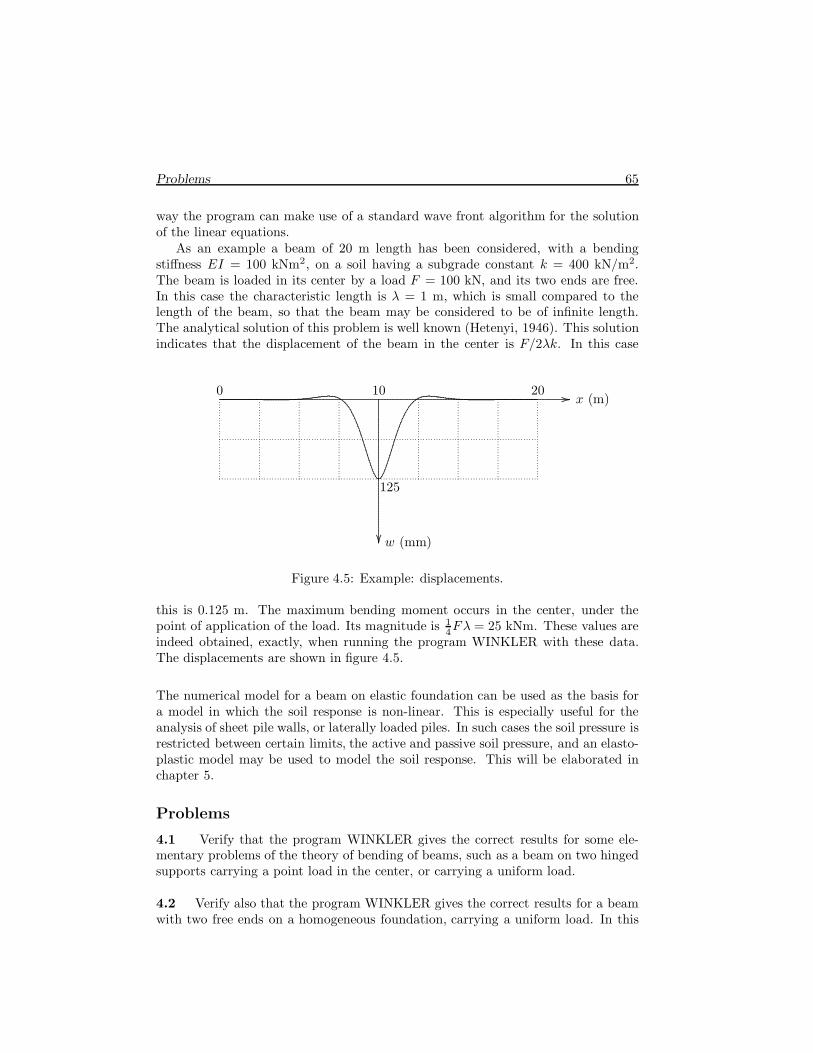
As an example a beam of 20 m length has been considered, with a bendingstiffness EI = 100 kNm2, on a soil having a subgrade constant k = 400 kN/m2.The beam is loaded in its center by a load F = 100 kN, and its two ends are free.In this case the characteristic length is λ = 1 m, which is small compared to thelength of the beam, so that the beam may be considered to be of infinite length.The analytical solution of this problem is well known (Hetenyi, 1946). This solutionindicates that the displacement of the beam in the center is F/2λk. In this case
..................................................................................................................................................................................................................................................................................................................................................................................................................................................................................................................................................................................................................................................................................................... ...............................................................................................................................................................................................................................................................................................................................
x (m)
w (mm)
0 10 20
125
............................................................................................................................................................................................................................................................................................................................................................................................................................................................................................................................................................................................................................................................................................................................................................................................................................................................................................................................................................................................................
........................................................................................................................
..........................................................................................................................
..
..
..
..
..
..
..
..
..
..
..
..
..
..
..
..
..
..
..
..
..
..
..
..
..
..
..
..
..
..
..
..
..
..
..
..
..
..
..
..
..
..
..
..
..
..
..
..
..
..
..
..
..
..
..
..
..
..
..
..
..
..
..
..
..
..
..
..
..
..
..
..
..
..
..
..
..
..
..
..
..
..
..
..
..
..
..
..
..
..
..
..
..
..
..
..
..
..
..
..
..
..
..
..
..
..
..
..
..
..
..
..
..
..
..
..
..
..
..
Figure 4.5: Example: displacements.
this is 0.125 m. The maximum bending moment occurs in the center, under thepoint of application of the load. Its magnitude is 1
4Fλ = 25 kNm. These values are
indeed obtained, exactly, when running the program WINKLER with these data.The displacements are shown in figure 4.5.
The numerical model for a beam on elastic foundation can be used as the basis fora model in which the soil response is non-linear. This is especially useful for theanalysis of sheet pile walls, or laterally loaded piles. In such cases the soil pressure isrestricted between certain limits, the active and passive soil pressure, and an elasto-plastic model may be used to model the soil response. This will be elaborated inchapter 5.
Problems
4.1 Verify that the program WINKLER gives the correct results for some ele-mentary problems of the theory of bending of beams, such as a beam on two hingedsupports carrying a point load in the center, or carrying a uniform load.
4.2 Verify also that the program WINKLER gives the correct results for a beamwith two free ends on a homogeneous foundation, carrying a uniform load. In this

66 Problems
case the bending moments must be zero, and the displacement must be constant,also if the beam is considered to consist of a number of sections of unequal length.
4.3 Compare the results obtained by the program WINKLER with analyticalsolutions for the case of a long beam on a homogeneous elastic foundation, with aforce or a moment at its end.
4.4 Modify the program WINKLER so that it shows the deflection curve and thebending moment in the form of a graph on the screen.
æ
Chapter 5
SHEET PILE WALLS
An interesting application of the theory of beams on elastic support, presented inthe previous chapter, is the analysis of a sheet pile wall. This requires an extensionof the theory to elasto-plastic supporting springs. The analysis is presented in thischapter, together with a simple computer program.
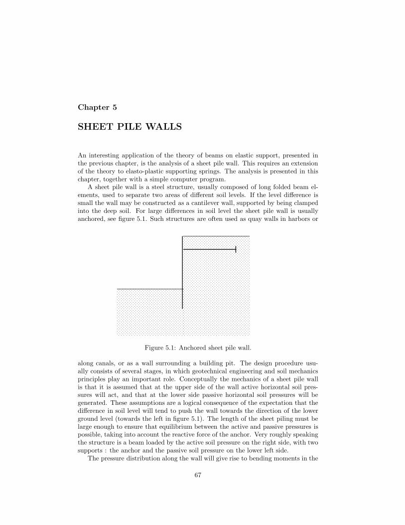
A sheet pile wall is a steel structure, usually composed of long folded beam el-ements, used to separate two areas of different soil levels. If the level difference issmall the wall may be constructed as a cantilever wall, supported by being clampedinto the deep soil. For large differences in soil level the sheet pile wall is usuallyanchored, see figure 5.1. Such structures are often used as quay walls in harbors or
...........................................................................................................................................................................................................................................................
...........................................................................................................................................................................................................................................................
. . . . . . . . . . . . . . . . . . . . . . . . .. . . . . . . . . . . . . . . . . . . . . . . . . .. . . . . . . . . . . . . . . . . . . . . . . . .. . . . . . . . . . . . . . . . . . . . . . . . . .. . . . . . . . . . . . . . . . . . . . . . . . .. . . . . . . . . . . . . . . . . . . . . . . . . .. . . . . . . . . . . . . . . . . . . . . . . . .. . . . . . . . . . . . . . . . . . . . . . . . . .. . . . . . . . . . . . . . . . . . . . . . . . .. . . . . . . . . . . . . . . . . . . . . . . . . .. . . . . . . . . . . . . . . . . . . . . . . . .. . . . . . . . . . . . . . . . . . . . . . . . . .. . . . . . . . . . . . . . . . . . . . . . . . .. . . . . . . . . . . . . . . . . . . . . . . . . .. . . . . . . . . . . . . . . . . . . . . . . . .. . . . . . . . . . . . . . . . . . . . . . . . . .. . . . . . . . . . . . . . . . . . . . . . . . .. . . . . . . . . . . . . . . . . . . . . . . . . .. . . . . . . . . . . . . . . . . . . . . . . . .. . . . . . . . . . . . . . . . . . . . . . . . . .. . . . . . . . . . . . . . . . . . . . . . . . .. . . . . . . . . . . . . . . . . . . . . . . . . .. . . . . . . . . . . . . . . . . . . . . . . . .. . . . . . . . . . . . . . . . . . . . . . . . . .. . . . . . . . . . . . . . . . . . . . . . . . .. . . . . . . . . . . . . . . . . . . . . . . . . .. . . . . . . . . . . . . . . . . . . . . . . . .. . . . . . . . . . . . . . . . . . . . . . . . . .. . . . . . . . . . . . . . . . . . . . . . . . .. . . . . . . . . . . . . . . . . . . . . . . . . .. . . . . . . . . . . . . . . . . . . . . . . . .. . . . . . . . . . . . . . . . . . . . . . . . . .. . . . . . . . . . . . . . . . . . . . . . . . .. . . . . . . . . . . . . . . . . . . . . . . . . .. . . . . . . . . . . . . . . . . . . . . . . . .. . . . . . . . . . . . . . . . . . . . . . . . . .
. . . . . . . . . . . . . . . . . . . . . . . . .. . . . . . . . . . . . . . . . . . . . . . . . . .. . . . . . . . . . . . . . . . . . . . . . . . .. . . . . . . . . . . . . . . . . . . . . . . . . .. . . . . . . . . . . . . . . . . . . . . . . . .. . . . . . . . . . . . . . . . . . . . . . . . . .. . . . . . . . . . . . . . . . . . . . . . . . .. . . . . . . . . . . . . . . . . . . . . . . . . .. . . . . . . . . . . . . . . . . . . . . . . . .. . . . . . . . . . . . . . . . . . . . . . . . . .. . . . . . . . . . . . . . . . . . . . . . . . .. . . . . . . . . . . . . . . . . . . . . . . . . .. . . . . . . . . . . . . . . . . . . . . . . . .. . . . . . . . . . . . . . . . . . . . . . . . . .. . . . . . . . . . . . . . . . . . . . . . . . .. . . . . . . . . . . . . . . . . . . . . . . . . .. . . . . . . . . . . . . . . . . . . . . . . . .. . . . . . . . . . . . . . . . . . . . . . . . . .. . . . . . . . . . . . . . . . . . . . . . . . .. . . . . . . . . . . . . . . . . . . . . . . . . .. . . . . . . . . . . . . . . . . . . . . . . . .. . . . . . . . . . . . . . . . . . . . . . . . . .. . . . . . . . . . . . . . . . . . . . . . . . .. . . . . . . . . . . . . . . . . . . . . . . . . .. . . . . . . . . . . . . . . . . . . . . . . . .. . . . . . . . . . . . . . . . . . . . . . . . . .. . . . . . . . . . . . . . . . . . . . . . . . .. . . . . . . . . . . . . . . . . . . . . . . . . .. . . . . . . . . . . . . . . . . . . . . . . . .. . . . . . . . . . . . . . . . . . . . . . . . . .. . . . . . . . . . . . . . . . . . . . . . . . .. . . . . . . . . . . . . . . . . . . . . . . . . .. . . . . . . . . . . . . . . . . . . . . . . . .. . . . . . . . . . . . . . . . . . . . . . . . . .. . . . . . . . . . . . . . . . . . . . . . . . .. . . . . . . . . . . . . . . . . . . . . . . . . .. . . . . . . . . . . . . . . . . . . . . . . . .. . . . . . . . . . . . . . . . . . . . . . . . . .. . . . . . . . . . . . . . . . . . . . . . . . .. . . . . . . . . . . . . . . . . . . . . . . . . .. . . . . . . . . . . . . . . . . . . . . . . . .. . . . . . . . . . . . . . . . . . . . . . . . . .. . . . . . . . . . . . . . . . . . . . . . . . .. . . . . . . . . . . . . . . . . . . . . . . . . .. . . . . . . . . . . . . . . . . . . . . . . . .. . . . . . . . . . . . . . . . . . . . . . . . . .. . . . . . . . . . . . . . . . . . . . . . . . .. . . . . . . . . . . . . . . . . . . . . . . . . .. . . . . . . . . . . . . . . . . . . . . . . . .. . . . . . . . . . . . . . . . . . . . . . . . . .. . . . . . . . . . . . . . . . . . . . . . . . .. . . . . . . . . . . . . . . . . . . . . . . . . .. . . . . . . . . . . . . . . . . . . . . . . . .. . . . . . . . . . . . . . . . . . . . . . . . . .. . . . . . . . . . . . . . . . . . . . . . . . .. . . . . . . . . . . . . . . . . . . . . . . . . .. . . . . . . . . . . . . . . . . . . . . . . . .. . . . . . . . . . . . . . . . . . . . . . . . . .. . . . . . . . . . . . . . . . . . . . . . . . .. . . . . . . . . . . . . . . . . . . . . . . . . .. . . . . . . . . . . . . . . . . . . . . . . . .. . . . . . . . . . . . . . . . . . . . . . . . . .. . . . . . . . . . . . . . . . . . . . . . . . .. . . . . . . . . . . . . . . . . . . . . . . . . .. . . . . . . . . . . . . . . . . . . . . . . . .. . . . . . . . . . . . . . . . . . . . . . . . . .. . . . . . . . . . . . . . . . . . . . . . . . .. . . . . . . . . . . . . . . . . . . . . . . . . .. . . . . . . . . . . . . . . . . . . . . . . . .. . . . . . . . . . . . . . . . . . . . . . . . . .. . . . . . . . . . . . . . . . . . . . . . . . .. . . . . . . . . . . . . . . . . . . . . . . . . .. . . . . . . . . . . . . . . . . . . . . . . . .. . . . . . . . . . . . . . . . . . . . . . . . . .. . . . . . . . . . . . . . . . . . . . . . . . .. . . . . . . . . . . . . . . . . . . . . . . . . .
Figure 5.1: Anchored sheet pile wall.
along canals, or as a wall surrounding a building pit. The design procedure usu-ally consists of several stages, in which geotechnical engineering and soil mechanicsprinciples play an important role. Conceptually the mechanics of a sheet pile wallis that it is assumed that at the upper side of the wall active horizontal soil pres-sures will act, and that at the lower side passive horizontal soil pressures will begenerated. These assumptions are a logical consequence of the expectation that thedifference in soil level will tend to push the wall towards the direction of the lowerground level (towards the left in figure 5.1). The length of the sheet piling must belarge enough to ensure that equilibrium between the active and passive pressures ispossible, taking into account the reactive force of the anchor. Very roughly speakingthe structure is a beam loaded by the active soil pressure on the right side, with twosupports : the anchor and the passive soil pressure on the lower left side.
The pressure distribution along the wall will give rise to bending moments in the
67

68 5. SHEET PILE WALLS
structure, and the steel profile of the wall must be chosen such that it can withstandthese bending moments. This involves an elementary calculation of the maximumstresses due to bending, and comparison of these stresses with the allowable stressesin various steel beam profiles.
The third phase of the design is the choice of the anchor, on the basis of theforce needed to maintain equilibrium. This involves the choice of the distance of theanchors, the length and depth of the individual anchors and the dimensions of theanchoring plates.
Various simplified calculation methods have been developed in geotechnical en-gineering, such as Blum’s method (Blum, 1931). In this chapter a more refinedmethod of analysis, using the theory of beams on an elasto-plastic foundation, ispresented.
It should be noted that in engineering design an important feature is the use ofsafety factors. These will not be considered here.
5.1 Description of the model
A numerical model for the analysis of a sheet pile wall can be developed from thenumerical model for a beam on elastic foundation, as presented in chapter 4. Thesoil response on both sides of the sheet pile wall is considered to consist of twoparts : one part proportional to the lateral displacement, and another constantpart. This enables to let the lateral soil pressure increase or decrease with thelateral displacement, with two limiting values : the active soil pressure as the lowerlimit, and the passive soil pressure as the upper limit.
The reaction of the soil is supposed to be elasto-plastic, as illustrated in figure 5.2.This figure represents the soil reaction from the soil to the right of the sheet pile
......................................................................................................................................................................................................................................................................................................................................................................................................................................................................................................................................................................................................................................... ...........................................................................................................................................................................................................................................................................................................
...................................................................................................................................... ................................................................................................................ ........... ................................................................................................................................................................................
..................................................................................................................................................................
........
........
........
........
........
........
..............
...........
.........................................................................
........
........
........
........
........
........
........
........
........
........
........
........
........
........
........
........
........
........
........
........
........
........
........
........
........
............
...........
...............................................................................................................................................................................................................................
....................................................................................... ........... ..................................................................................................
............
........................................
........
........
........
........
........
........
........
........
........
........
........
........
........
........
........
........
........
........
........
........
........
........
........
........
vi
Ri
Kaσ′v − 2c
√Ka
Kpσ′v + 2c
√Kp
∆v
Figure 5.2: Elasto-plastic soil response, right side.
wall, assuming that the positive direction of the displacements is towards the right.The soil reaction is elastic if the displacement of the wall is small, and plastic ifthe displacement exceeds a certain value, generating active earth pressure if the

5.1. Description of the model 69
displacement is to the left, and passive earth pressure if the displacement is to theright. In repeated loading and unloading the elastic branch of the soil response isrelocated, depending upon the accumulated plastic deformation. In general the soilresponse may be written as
Ri = Si(vi − vi) + Ti, (5.1)
where vi is the displacement of element i, which may be related to the displacementsof the nodes by
vi = 12(ui + ui−1). (5.2)
In eq. (5.1) vi is the accumulated plastic displacement, which must be updated duringthe deformation process. The coefficient Si represents the slope of the response curve,which is zero in the plastic branches. The term Ti is zero in the elastic branch, andmay be used to represent the plastic soil response in the plastic branches.
The maximum lateral earth pressure is the passive earth pressure, for whichelementary soil mechanics gives the value
σ′p = Kpσ
′v + 2c
√Kp, (5.3)
where σ′v is the vertical effective stress, c is the cohesion, and Kp is the passiveearth pressure coefficient, which is related to the friction angle φ by the relation
Kp =1 + sin φ
1 − sin φ. (5.4)
The minimum lateral earth pressure is the active earth pressure, which is given inbasic soil mechanics texts as
σ′a = Kaσ′
v − 2c√
Kp. (5.5)
Here Ka is the passive earth pressure coefficient,
Ka =1 − sin φ
1 + sin φ. (5.6)
Usually the active earth pressure is limited from below by requiring that the effectivestress cannot be negative,
σ′a ≥ 0. (5.7)
The lateral pressure in the case of zero displacement is assumed to be defined by thecoefficient of neutral earth pressure K0,
σ′0 = K0σ
′v. (5.8)
It should be noted that there is also a response on the other side of the wall.This is of the same type as the response on the right side, except for the sign, seefigure 5.3. Initially, for very small displacements, the two responses will both be inthe elastic range, and this simply means that the stiffnesses can be added. After
70 5. SHEET PILE WALLS
......................................................................................................................................................................................................................................................................................................................................................................................................................................................................................................................................................................................................................................... ...........................................................................................................................................................................................................................................................................................................
................................................................... ........................................................................................................................... ........... .........
.........................................................................................................................................................................................................................................................................................................................................
........
........
........
........
........
........
........
........
........
........
........
........
........
........
........
........
........
........
........
........
........
........
........
........
........
............
...........
...............................................................................................................................................................................................................................
........
........
........
........
........
........
..............
...........
.........................................................................
....................................................................................... ........... ..................................................................................................
.......................
................................... ........................................................................................................................................
........
........
........
........
........
........
........
vi
−Ri
Kpσ′v + 2c
√Kp
Kaσ′v − 2c
√Ka
∆v
Figure 5.3: Elasto-plastic soil response, left side.
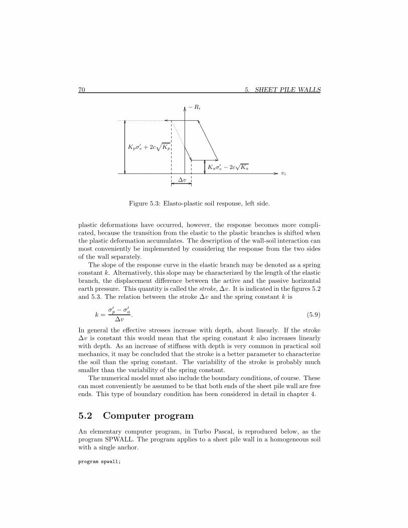
plastic deformations have occurred, however, the response becomes more compli-cated, because the transition from the elastic to the plastic branches is shifted whenthe plastic deformation accumulates. The description of the wall-soil interaction canmost conveniently be implemented by considering the response from the two sidesof the wall separately.
The slope of the response curve in the elastic branch may be denoted as a springconstant k. Alternatively, this slope may be characterized by the length of the elasticbranch, the displacement difference between the active and the passive horizontalearth pressure. This quantity is called the stroke, ∆v. It is indicated in the figures 5.2and 5.3. The relation between the stroke ∆v and the spring constant k is
k =σ′
p − σ′a
∆v. (5.9)
In general the effective stresses increase with depth, about linearly. If the stroke∆v is constant this would mean that the spring constant k also increases linearlywith depth. As an increase of stiffness with depth is very common in practical soilmechanics, it may be concluded that the stroke is a better parameter to characterizethe soil than the spring constant. The variability of the stroke is probably muchsmaller than the variability of the spring constant.
The numerical model must also include the boundary conditions, of course. Thesecan most conveniently be assumed to be that both ends of the sheet pile wall are freeends. This type of boundary condition has been considered in detail in chapter 4.
5.2 Computer program
An elementary computer program, in Turbo Pascal, is reproduced below, as theprogram SPWALL. The program applies to a sheet pile wall in a homogeneous soilwith a single anchor.
program spwall;
5.2. Computer program 71
uses crt;
const
nn=100;zz=4;ni=100;
var
len,dep,anc,stf,wht,act,pas,neu,coh,stk,ei,ft,dz,cp:real;
n,i,ll,lp,nerr,mp,mq,plast,it:integer;
z,s,d,f,u,q,ul,ur,m,ff:array[0..nn] of real;
asl,psl,sll,pal,ppl,pnl:array[1..nn] of real;
asr,psr,slr,par,ppr,pnr:array[1..nn] of real;
p:array[0..nn,1..zz,1..2,1..2] of real;
kk:array[0..nn,1..zz] of integer;
g:array[1..2,1..2] of real;
tr,tl:array[0..nn] of integer;
fs,wt:array[0..100] of real;data:text;
procedure title;
begin
clrscr;gotoxy(37,1);textbackground(7);textcolor(0);write(’ SPWALL ’);
textbackground(0);textcolor(7);writeln;writeln;
end;
procedure next;
var
a:char;
begin
gotoxy(25,25);textbackground(7);textcolor(0);
write(’ Touch any key to continue ’);write(chr(8));
a:=readkey;textbackground(0);textcolor(7)
end;
procedure input;
begin
title;
writeln(’This is a program for the analysis of a sheet pile wall.’);
writeln;
write(’Length of the wall (m) ......... ’);readln(len);
write(’Depth of excavation (m) ........ ’);readln(dep);
write(’Depth of anchor point (m) ...... ’);readln(anc);
write(’Stiffness of anchor (kN/m) ..... ’);readln(stf);
write(’Unit weight of soil (kN/m3) .... ’);readln(wht);
write(’Active pressure coefficient .... ’);readln(act);
write(’Passive pressure coefficient ... ’);readln(pas);
write(’Neutral pressure coefficient ... ’);readln(neu);
write(’Cohesion (kN/m2) ............... ’);readln(coh);
write(’Total stroke (m) ............... ’);readln(stk);
write(’Stiffness EI (kNm2) ............ ’);readln(ei);
write(’Number of elements (max. 100) .. ’);readln(n);
if n<10 then n:=10;if n>nn then n:=nn;
if act>1 then act:=1;if pas<1 then pas:=1;
if neu<act then neu:=act;if neu>pas then neu:=pas;
ft:=0;dz:=len/n;z[0]:=0;u[0]:=0;m[0]:=0;ul[0]:=0;ur[0]:=0;
for i:=1 to n do
begin
z[i]:=z[i-1]+dz;d[i]:=dz;tr[i]:=0;tl[i]:=0;
u[i]:=0;m[i]:=0;ul[i]:=0;ur[i]:=0;
end;
end;
procedure constants;
var

72 5. SHEET PILE WALLS
szr,szl,e:real;
begin
for i:=1 to n do
begin
e:=0.001;szr:=wht*(z[i]-d[i]);if szr<e then szr:=e;
par[i]:=act*szr-2*coh*sqrt(act);if par[i]<0 then par[i]:=0;
pnr[i]:=neu*szr;ppr[i]:=pas*szr+2*coh*sqrt(pas);
if ppr[i]<par[i]+e then ppr[i]:=par[i]+e;
asr[i]:=(pnr[i]-par[i])*stk/(ppr[i]-par[i]);
psr[i]:=(ppr[i]-pnr[i])*stk/(ppr[i]-par[i]);
slr[i]:=(ppr[i]-par[i])/stk;
szl:=wht*(z[i]-d[i]-dep);if szl<e then szl:=e;
pal[i]:=act*szl-2*coh*sqrt(act);if pal[i]<0 then pal[i]:=0;
pnl[i]:=neu*szl;ppl[i]:=pas*szl+2*coh*sqrt(pas);
if ppl[i]<pal[i]+e then ppl[i]:=pal[i]+e;
asl[i]:=(pnl[i]-pal[i])*stk/(ppl[i]-pal[i]);
psl[i]:=(ppl[i]-pnl[i])*stk/(ppl[i]-pal[i]);
sll[i]:=(ppl[i]-pal[i])/stk;
end;
end;
procedure springs;
var
i,nr,ll:integer;
um,sp,eps,sx:real;
begin
nerr:=0;plast:=0;eps:=0.000001;ll:=0;
for i:=1 to n do
begin
um:=(u[i]+u[i-1])/2;if um-ul[i]>asl[i]+eps then
begin sx:=pal[i];sp:=0;nr:=1;plast:=plast+1;end
else if um-ul[i]<-psl[i]-eps then
begin sx:=ppl[i];sp:=0;nr:=-1;plast:=plast+1;end
else begin sp:=sll[i];sx:=pnl[i]+sp*ul[i];nr:=0;end;
f[i]:=sx*d[i];s[i]:=sp*d[i];
if tl[i]<>nr then begin tl[i]:=nr;nerr:=nerr+1;end;
if um-ur[i]<-asr[i]-eps then
begin sx:=par[i];sp:=0;nr:=1;plast:=plast+1;end
else if um-ur[i]>psr[i]+eps then
begin sx:=ppr[i];sp:=0;nr:=-1;plast:=plast+1;end
else begin sp:=slr[i];sx:=pnr[i]-sp*ur[i];nr:=0;end;
f[i]:=f[i]-sx*d[i];s[i]:=s[i]+sp*d[i];
if tr[i]<>nr then begin tr[i]:=nr;nerr:=nerr+1;end;
if (z[i]>anc-d[i]/2) and (ll=0) then
begin ll:=1;s[i]:=s[i]+stf;end;
end;
end;
procedure matrix;
var
i,j,k,l:integer;a1,a2,b1,b2,c1:real;
begin
for i:=0 to n do for j:=1 to zz do
begin
kk[i,j]:=0;
for k:=1 to 2 do for l:=1 to 2 do p[i,j,k,l]:=0;
end;
for i:=1 to n-1 do

5.2. Computer program 73
begin
kk[i,1]:=i;kk[i,2]:=i-1;kk[i,3]:=i+1;kk[i,zz]:=3;
end;
kk[0,1]:=0;kk[0,2]:=1;kk[0,zz]:=2;
kk[n,1]:=n;kk[n,2]:=n-1;kk[n,zz]:=2;
for i:=1 to n-1 do
begin
a1:=1/d[i+1];a2:=1/d[i];
p[i,1,1,1]:=-a1-a2;p[i,2,1,1]:=a2;p[i,3,1,1]:=a1;
p[i,1,1,2]:=-(s[i]+s[i+1])/4;p[i,2,1,2]:=-s[i]/4;
p[i,3,1,2]:=-s[i+1]/4;
p[i,zz,1,1]:=-(f[i]+f[i+1])/2;
p[i,1,2,2]:=-a1-a2;p[i,2,2,2]:=a2;p[i,3,2,2]:=a1;
p[i,1,2,1]:=(d[i]+d[i+1])/(4*ei);
p[i,2,2,1]:=d[i]/(4*ei);p[i,3,2,1]:=d[i+1]/(4*ei);
end;
p[0,1,1,1]:=1;p[0,zz,1,1]:=0;
p[0,1,2,2]:=1;p[0,2,2,2]:=s[1]/2;
p[0,1,2,1]:=2/d[1];p[0,2,2,1]:=-2/d[1];
p[0,zz,2,2]:=f[1];
p[n,1,1,1]:=1;p[n,zz,1,1]:=0;
p[n,1,2,2]:=s[n]/2;p[n,2,2,2]:=s[n]/2;
p[n,1,2,1]:=2/d[n];p[n,2,2,1]:=-2/d[n];
p[n,zz,2,2]:=f[n];
end;
procedure solve;
var
i,j,k,l,ii,ij,ik,jj,jk,jl,jv,kc,kv,lv:integer;
cc,aa:real;
begin
for i:=n downto 0 do
begin
kc:=kk[i,zz];for kv:=1 to 2 do
begin
if p[i,1,kv,kv]=0 then
begin
writeln(’Error : no equilibrium possible’);halt;
end;
cc:=1.0/p[i,1,kv,kv];
for ii:=1 to kc do for lv:=1 to 2 do
begin
p[i,ii,kv,lv]:=cc*p[i,ii,kv,lv];
end;
p[i,zz,kv,kv]:=cc*p[i,zz,kv,kv];
for lv:=1 to 2 do if (lv<>kv) then
begin
cc:=p[i,1,lv,kv];
for ii:=1 to kc do for ij:=1 to 2 do
begin
p[i,ii,lv,ij]:=p[i,ii,lv,ij]-cc*p[i,ii,kv,ij];
end;
p[i,zz,lv,lv]:=p[i,zz,lv,lv]-cc*p[i,zz,kv,kv];
end;
end;
if kc>1 then
begin

74 5. SHEET PILE WALLS
for j:=2 to kc do
begin
jj:=kk[i,j];l:=kk[jj,zz];jk:=l;
for jl:=2 to l do begin if kk[jj,jl]=i then jk:=jl;end;
for kv:=1 to 2 do for lv:=1 to 2 do g[kv,lv]:=p[jj,jk,kv,lv];
kk[jj,jk]:=kk[jj,l];kk[jj,l]:=0;
for kv:=1 to 2 do for lv:=1 to 2 do
begin
p[jj,jk,kv,lv]:=p[jj,l,kv,lv];p[jj,l,kv,lv]:=0;
p[jj,zz,lv,lv]:=p[jj,zz,lv,lv]-g[lv,kv]*p[i,zz,kv,kv];
end;
l:=l-1;kk[jj,zz]:=l;
for ii:=2 to kc do
begin
ij:=0;
for ik:=1 to l do
begin
if kk[jj,ik]=kk[i,ii] then ij:=ik;
end;
if ij=0 then
begin
l:=l+1;ij:=l;kk[jj,zz]:=l;kk[jj,ij]:=kk[i,ii];
end;
for kv:=1 to 2 do for lv:=1 to 2 do for jv:=1 to 2 do
p[jj,ij,kv,lv]:=p[jj,ij,kv,lv]-g[kv,jv]*p[i,ii,jv,lv];
end;
end;
end;
end;
for j:=0 to n do
begin
l:=kk[j,zz];if l>1 then
begin
for k:=2 to l do
begin
jj:=kk[j,k];
for kv:=1 to 2 do for lv:=1 to 2 do
p[j,zz,kv,kv]:=p[j,zz,kv,kv]-p[j,k,kv,lv]*p[jj,zz,lv,lv];
end;
end;
end;
for i:=0 to n do begin m[i]:=p[i,zz,1,1];u[i]:=p[i,zz,2,2];end;
q[0]:=0;ff[0]:=0;for i:=1 to n do
begin
aa:=(m[i]-m[i-1])/d[i];
q[i]:=-q[i-1]+2*aa;ff[i]:=(q[i-1]-q[i])/d[i];
end;
end;
begin
input;constants;title;springs;it:=0;
repeat
matrix;solve;springs;
writeln(’Number of plastic springs .......... ’,plast);
writeln(’Displacement at the top (m) ........ ’,u[0]:8:6);
if plast=2*n then begin writeln(’Pile failed’);nerr:=0;end;
it:=it+1;if it=ni then

5.2. Computer program 75
begin
writeln(’Warning : no convergence ’);writeln;nerr:=0;
end;
until nerr=0;
if plast<2*n then
begin
title;ll:=0;
writeln(’ z u M Q f’);
for i:=0 to n do
begin
writeln(z[i]:8:3,u[i]:10:3,m[i]:10:3,q[i]:10:3,ff[i]:10:3);
ll:=ll+1;if (ll=20) then
begin
next;title;ll:=0;
writeln(’ z u M Q f’);
end;
end;
next;title;
end;
end.
Program SPWALL.
The program runs interactively, and will present information about its operationand input data automatically. The program is a straightforward extension of theprogram WINKLER, presented in chapter 4. The main extension is that the soilreaction consists of reactions on the left side as well as the right side. It is assumedin the program that the soil is fully homogeneous, and that the soil surface at theleft side is lowered by excavation. The program calculates the deformations due tothis excavation. In the program the parameters tr[i] and tl[i] indicate the stateof the springs in node i at the right side and the left side, respectively. If its valueis 0 the spring is in the elastic range, if its value is +1 the spring is in the activestate, and if its value is -1 the spring is in the passive state. Initially all springs areassumed to be in the elastic range. After calculating all displacements the programchecks whether these assumptions were correct, and if necessary corrects them andrepeats the calculations.
The soil response is characterized by the neutral, active and passive soil pressurecoefficients, the cohesion, the weight of the material, and a characteristic displace-ment, the stroke, which represents the displacement difference between the states ofactive and passive lateral stress, see also figures 5.2 and 5.3. Output consists of alist on the screen of the lateral displacement, the bending moment, the shear force,and the resultant lateral load, all as a function of depth. More advanced outputfeatures, such as graphical facilities, may be added by the user.
Example
As an example some results are shown for a sheet pile wall with the following data.
len = 15
dep = 10

76 5. SHEET PILE WALLS
anc = 2
stf = 10000
wht = 20
act = 0.3333
pas = 3.0000
neu = 1.0000
coh = 0
stk = 0.02
ei = 100000
n = 100
Data for example 1.
This example refers to an excavation of 10 m depth in sand. The length of the sheetpile wall is 15 m, and the anchor is located at a depth of 2 m. The data for the soil,the sheet pile wall and the anchor are given in the table. Some of the results areshown in figure 5.4, in the form of a graph of the resultant horizontal stresses acting
............................................................................................................................................................................................................................................................................................................................................................................................................................................................................................................................................................................................................................................................................................................................................................................................... .............................................................................................................................................................................................................................................................................................................................................................................................................................................................................................................................................................................................................
f (kN/m2)
z (m)
−100 0 100 200 300
5
10
15
...................................................................................................................................................................................................................................................................................................................................................................................................................................................................................................................................................................................................................................................................................................................................................................................................................................................................................................................................................................................................................................................................................................................................................................................................................................................................................................................................................................................................................................................................
.......................................................................................................................................
.......................................................................................................................................
.......................................................................................................................................
.......................................................................................................................................
.......................................................................................................................................
.......................................................................................................................................
.......................................................................................................................................
.......................................................................................................................................
.......................................................................................................................................
.......................................................................................................................................
.......................................................................................................................................
.......................................................................................................................................
.......................................................................................................................................
.......................................................................................................................................
.......................................................................................................................................
..........................................................................................
..........................................................................................
..........................................................................................
..........................................................................................
..........................................................................................
..........................................................................................
..........................................................................................
..........................................................................................
..........................................................................................
Figure 5.4: Resultant horizontal stresses.
on the wall. It appears that in the top 10 meters the lateral soil pressure is theactive soil pressure from the right, and below that level the passive pressure fromthe left starts to dominate, as seems natural. In the top part of the wall the pressureappears to be somewhat larger. The displacements of the stiff wall are to the rightthere, because of the effect of the anchor, so that larger horizontal pressures aregenerated. At the lower end of the wall it appears that a very high pressure fromthe right side of the wall is generated. Again this must be due to deformations
Problems 77
towards the right. This phenomenon is taken into account in Blum’s simplifiedmethod, by an equivalent concentrated force (Blum, 1931). The occurrence of thisforce at the bottom of the sheet pile wall in the numerical model may be consideredas a confirmation of the validity of Blum’s original assumption.
The program SPWALL may be used as the basis of programs with more ad-vanced features, such as a sheet pile wall with several anchors in a layered soil, withcomplex loading and excavation histories. Such programs are distributed by variouscompanies and institutes.
Problems
5.1 Run the program SPWALL with the data of example 1, given above. Alsorun the program with modified data, for instance by taking a different value for thestroke. Show that Blum’s concentrated force occurs only if the stroke is relativelysmall, which indicates a stiff soil.
5.2 Compare the results obtained by the program SPWALL with results obtainedby Blum’s method, if this method is available.
5.3 Modify the program SPWALL so that it shows the deflection curve, the bend-ing moment, the shear force, and the lateral stress in the form of graphs on the screen.
æ