Shear-flexible finite-element models of laminated ... · nasa technical note d a 0 7 n z c -loan...

N A S A TECHNICAL NOTE

d a 0 7 n z c

-LOAN COPY: RETURN TO 4 FWL TECHNICAL LIBRARY

KIRTLAND AFB, M. M.

SHEAR-FLEXIBLE FINITE-ELEMENT MODELS OF LAMINATED COMPOSITE PLATES A N D SHELLS

Ahmed K . Noor utzd Michael D. Mnthers

Lnrzgley Reseccrch Ceizter Hu?~pto 12, vu. 23 665

N A T I O N A L AERONAUTICS A N D SPACE A D M I N I S T R A T I O N W A S H I N G T O N , D. C. DECEMBER 1975

I

https://ntrs.nasa.gov/search.jsp?R=19760007434 2018-08-31T18:54:02+00:00Z

- -_ - . . . -~ 2. Sovernment Accession No.

- - 5. Report Date , December 1975

1 L-10414

1 q e w r t No

~

NASA TN D-8044 4. Title and Subtitle

SHEAR-FLEXIBLE FINITE-ELEMENT MODELS O F 6. Performing Organization Code

LAMINATED COMPOSITE PLATES AND SHELLS . ._ ~

7. Author(s) 8. Performing Organizdticn Report No.

. .~ - Ahmed K. Noor and Michael D. Mathers .... . " _ .. ~ 10. Work Unit No.

9. Performing OrydniLarim Ndmr dnd Addre; . . 506-17-21-02 .. ______-

Contract or Grant No.

_ _ ,

NASA Langley Research Center Hampton, Va. 23665

. . . ~ . . . _ 15. Sbpplementary Notes

Ahmed K. Noor and Michael D. Mathers: The George Washington University, Joint Institute for Acoustics and Flight Sciences.

.___ . .. . . ~ ~. . . . ~ ._ - . -_ ~- . 16 Abstrdct

13. Type of Report dnd Period Covered

Technical Note - . . . . . . . . __ ._

14. Sponsoring Ayeniy %de

. - - . . . -.

12 S&wiwring Ayeniy Name and Address

National Aeronautics and Space Administration

Several finite-element models are applied to the linear static, stability, and vibration analysis of laminated composite plates and shells. shallow-shell theory, with the effects of shear deformation, anisotropic material behavior, and bending-extensional coupling included. finite-element models are considered. Discussion is focused on the effects of shear deformation and anisotropic material behavior on the accuracy and convergence of different finite-element models. of (a) increasing the order of the approximating polynomials, (b) adding internal degrees of freedom, and (c) using derivatives of generalized displacements as nodal parameters.

The study is based on linear

Both stiffness (displacement) and mixed

Numerical studies are presented which show the effects

20. Security Classif. (of this page)

Unclassified -- I 19. Security Classif. (of this report)

Unclassified

- . . 17. Key-Words (Suggested by Author(s) )

Finite elements Laminates

21. NO. of Pages 22. Price'

111 $5.25

- - 18. Distribution Statement c Unclassified -- Unlimited

I Fibrous composites Stress analysis Anisotropy Stability - _ Shells Plates I Vibrations

Shear deformation Subject Category 3 9

For sale by the National Technical Information Service, Springfield, Virginia 221 61

CONTENTS

SUMMARY . . . . . . . . . . . . . . . . . . . . . . . . . . . . . . . . 1

INTRODUCTION . . . . . . . . . . . . . . . . . . . . . . . . . . . . . 1

SYMBOLS AND NOTATION . . . . . . . . . . . . . . . . . . . . . . . . 2

MATHEMATICAL FORMULATION . . . . . . . . . . . . . . . . . . . . . . 6 FINITE-ELEMENT DISCRETIZATION . . . . . . . . . . . . . . . . . . . . 8 ELEMENT-BEHAVIOR REPRESENTATION . . . . . . . . . . . . . . . . . 9 FINITE-ELEMENT EQUATIONS . . . . . . . . . . . . . . . . . . . . . . 10 BOUNDARY CONDITIONS . . . . . . . . . . . . . . . . . . . . . . . . 11 ASSEMBLY AND SOLUTION OF EQUATIONS . . . . . . . . . . . . . . . 13 EIGENVALUE EXTRACTION TECHNIQUES . . . . . . . . . . . . . . . . . 14 EVALUATION OF STRESS RESULTANTS . . . . . . . . . . . . . . . . . 14

NUMERICALSTUDIES . . . . . . . . . . . . . . . . . . . . . . . . . . . 15 PLATE EVALUATION RESULTS . . . . . . . . . . . . . . . . . . . . . 15

Square Plates . . . . . . . . . . . . . . . . . . . . . . . . . . . . . 16 Simply Supported Orthotropic Plates . . . . . . . . . . . . . . . . . . 16 Clamped Plates . . . . . . . . . . . . . . . . . . . . . . . . . . . 20 Anisotropic Plates . . . . . . . . . . . . . . . . . . . . . . . . . . . 20

Skew Plates . . . . . . . . . . . . . . . . . . . . . . . . . . . . . . 21 SHELL EVALUATION RESULTS . . . . . . . . . . . . . . . . . . . . . 22

Shallow Spherical Shells . . . . . . . . . . . . . . . . . . . . . . . . . 22

__

Orthotropic Shallow Shells . . . . . . . . . . . . . . . . . . . . . . . 23 Anisotropic Shallow Shells . . . . . . . . . . . . . . . . . . . . . . . 24 Rigid Body Modes . . . . . . . . . . . . . . . . . . . . . . . . . . 24

Cylindrical Shells . . . . . . . . . . . . . . . . . . . . . . . . . . . . 25

Orthotropic Cylinders . . . . . . . . . . . . . . . . . . . . . . . . . 26 Anisotropic Cylinders . . . . . . . . . . . . . . . . . . . . . . . . . 27

CONCLUDING REMARKS . . . . . . . . . . . . . . . . . . . . . . . . . 27

. __ Isotropic Cylinder With a Circular Cutout . . . . . . . . . . . . . . . . 25

APPENDIX A . FUNDAMENTAL EQUATIONS OF SHEAR-DEFORMATION . . . . .. __ .

SHALLOW-SHELL THEORY . . . . . . . . . . . . . . . . . . . . . . . . 29 STRAIN-DISPLACEMENT RELATIONSHIPS I . . . . . . . . . . . . . . . . 29 CONSTITUTIVE RELATIONS O F THE SHELL . . . . . . . . . . . . . . . 29

... 111

I

APPENDIX-B _- ELASTIC- COEFFICIENTS O F LAMINATED SHELLS . ELASTIC STIFFNESSES O F THE LAYERS . . . . . . . . . . . ELASTIC COEFFICIENTS OF THE SHELL . . . . . . . . . . .

APPENDIX C . SHAPE FUNCTIONS-USED IN PRESENT STUDY . . QUADRILATERAL ELEMENTS . . . . . . . . . . . . . . . .

Bilinear Shape Functions . . . . . . . . . . . . . . . . . . Quadratic Shape Functions . . . . . . . . . . . . . . . . . Cubic Shape Functions . . . . . . . . . . . . . . . . . . . Hermitian Shape Functions . . . . . . . . . . . . . . . . .

Elements SQ5 and SQ9 . . . . . . . . . . . . . . . . . . Elements SQ7 and SQ11 . . . . . . . . . . . . . . . . .

TRIANGULAR ELEMENTS . . . . . . . . . . . . . . . . . . Linear Shape Functions . . . . . . . . . . . . . . . . . . . Quadratic Shape Functions . . . . . . . . . . . . . . . . . Cubic Shape Functions . . . . . . . . . . . . . . . . . . .

EQUATIONS FOR INDIVIDUAL ELEMENTS . . . . . . . . . .

__ .

Shape Functions Associated With Nodeless . . Variables (Bubble Modes) ___ .

..

APPENDIX D :FORMULAS FOR CO_EFFICIENTS IN- GOVERNING

. . . . .

REFERENCES . . . . . . . . . . . . . . . . . .

TABLES . . . . . . . . . . . . . . . . . . . .

FIGURES . . .

. . . . . . .

. . . . . . .

. . . . . . . . . . . . . . . . . . . . . . . .

. . . . . . 31

. . . . . . 31

. . . . . . 32

. . . . . . 34

. . . . . . 34

. . . . . . 34

. . . . . . 34

. . . . . . 35

. . . . . . 35

. . . . . . 36

. . . . . . 36

. . . . . . 37

. . . . . . 37

. . . . 37

. . . . 37

. . . . . . 38

. . . . . . 39

. . . . . . 42

. . . . . . 46

. . . . . . 67

iv

SHEAR-FLEXIBLE FINITE-ELEMENT MODELS OF LAMINATED

COMPOSITE PLATES AND SHELLS

Ahmed K. Noor* and Michael D. Mathers" Langley Research Center

SUMMARY

Several finite-element models are applied to the linear static, stability, and vibration analy- The study is based on linear shallow-shell theory, sis of laminated composite plates and shells.

with the effects of shear deformation, anisotropic material behavior, and bending-extensional coupling included. Discussion is focused on the effects of shear deformation and anisotropic material behavior on the accuracy and convergence of different finite-element models. Numerical studies are presented which show the effects of (a) increasing the order of the approximating polynomials, (b) adding internal degrees of freedom, and (c) using derivatives of generalized displacements as nodal parameters.

Both stiffness (displacement) and mixed finite-element models are considered.

IbJTRODUCTION

Although the finite-element analysis of isotropic plates and shells has received considerable attention in the literature, investigations of laminated composite plates and shells are rather limited in extent. fibrous composite plates and shells often requires inclusion of the transverse shear effects in their mathematical models. This fact has been amply documented for linear static, stability, and dynamic problems. (See, for example, refs. 1 to 5 . )

The reliable prediction of the response characteristics of high-modulus

At present there are three approaches for developing plate and shell finiteelement models which account for shear deformation. dimensional isoparametric solid elements which automatically include the shear-distortion mecha- nism (refs. 6 and 7). The second approach employs two-dimensional elements used with independent shape (or interpolation) functions for displacements and rotations (refs. 8 and 9). The third approach is based on the addition of effects of shear deformation to two-dimensional classical plate or shell elements through the use of equilibrium equations (refs. 10 and 11). Although it is desirable to have an element which gives accurate results regardless of how important the shear deformation is, most of the existing elements do not satisfy this requirement.

The first approach is based on the use of three-

.

*The George Washington University, Joint Institute for Acoustics and Flight Sciences.

In the context. of the stiffness method, the first approach has the major disadvantage that it leads to a stiffness matrix which is (1) very large for laminated composites consisting of many layers and (2) highly ill conditioned for thin plates or shells. tion polynomials are used, the second approach leads to overly stiff elements for very thin plates and shells. Although the aforementioned drawbacks have been recognized and some improvements have been suggested, the difficulties have not been overcome. refs. 12 to 17.) The range of validity of the third approach has not been explored. Since the second approach provides flexibility and simplicity in fulfilling the interelement compati- bility conditions and does not result in as large a stiffness matrix as in the first approach, it was adopted in the present study.

If low-order interpola-

(See, e.g.,

The first objective of this paper is to assess the relative merits of a number of displacement and mixed shear-flexible finite elements when applied to the linear static, stability, and vibration problems of laminated plates and shells. Emphasis is focused on the effects of shear deformation and anisotropic material behavior on the accuracy and convergence of the different models. The second objective is t o study the effects of increasing the order of approximating polynomials, adding internal degrees of freedom, and using derivatives of generalized displacements as nodal parameters on the accuracy and rate of convergence of the different models. To the authors’ knowledge no publication exists in which the aforementioned effects are studied in any detail.

The analytical formulation is based on a form of the shallow-shell theory modified to include the effects of shear deformation and rotary inertia. au t this paper since it is particularly useful in identifying the symmetries and, consequently, simplifies the element development.

of the fundamental unknowns).

Indicia1 notation is used through-

Both triangular and quadrilateral elements are considered. The elements are conforming and satisfy continuity requirements of the type C 0 (continuity

SYMBOLS AND NOTATION

Aaprp 9Aa3p3’ shell compliance coefficients, inverse of shell stiffnesses

B@YP,G&P i a side length of plate or shallow shell

extensional stiffnesses of shell ColpYP

transverse shear stiffnesses of shell ca3p3

stiffness coefficients of kth layer of shell

portions of shell boundary over which tractions and displacements are prescribed

bending stiffnesses of shell

elastic modulus of isotropic materials

error index (see eq. (36))

elastic moduli in direction of fibers and normal to it, respectively

stiffness interaction coefficients of shell

rise of shallow shells

shear moduli in plane of fibers and normal to it, respectively

nodal stress resultants

local thickness of shell

distances from reference (middle) surface to top and bottom surfaces of kth layer, respectively

stiffness coefficients of shell element

geometric or initial stress stiffness coefficients of shell element

curvatures and twist of shell reference surface

direction cosines, cos(xa,xal)

consistent mass coefficients of shell element

bending-moment stress resultants

number of shape functions

densitv parameters of shell

3

I1

- n

P f

PO

Qa

R

r

ij -ij s- s - IJ’ IJ

T

U

UC

UO

‘shyUa

shape or interpolation functions

extensional (in-plane) stress resultants

relative magnitudes of prestress components

total number of elements in X I - or x2direction

total number of nodes in finite-element model

unit outward normal to shell boundary

consistent nodal load coefficients

external load intensities in coordinate directions

intensity of uniform pressure loading

transverse shear stress resultants

radius of curvature

radial coordinate in circular cylindrical shell (see fig. 24)

“generalized” stiffness coefficients of shell element

kinetic energy of shell

strain energy of shell

complementary energy of shell

strain energy due to prestress

measures of shear deformation and degree of anisotropy

displacement components in coordinate directions

work done by internal forces

4

W,W work done by external forces

orthogonal curvilinear coordinate system (see fig. 1 ) xQI,x3

1 xor nodal values of x,

- P dimensionless eigenvalues of stiffness matrix

relative size of rth element in variable grid (eq. (37))

dummy coordinates of ends of rth element

e fiber orientation, angle between fiber direction and x1 -axis

constant defined in appendix D K

h in-plane loading parameter

- - - __ __ nondimensional frequency ( w \i pa ET for plates; w \/ph2/ET for shallow

spherical segments; o \/*; for circular cylinders)

- x

Poisson’s ratio for isotropic materials V

Poisson’s ratio measuring strain in T-direction (transverse) due to uniaxial normal stress in L-direction (direction of fibers)

LT

natural coordinates of node i

natural (dimensionless) coordinate system in element domain

functionals defined in equations (1) and (2)

density of plate or shell material

density of kth layer of laminated shell

uniform extensional stress . in cylindrical shell

rotation components

5

_. . .. . .

nodal displacement parameters 4 s2 shell domain

0 circular frequency of vibration of shell

Range of indices:

Lowercase Latin indices 1 to m

Uppercase Latin indices: I,J 1 to 5 I,J 1 to 8 - -

Greek indices 1,2

Finite-element-model notation:

SQN stiffness formulation, quadrilateral element, N shape functions per fundamental unknown

STN

MQN

MTN

SQH

stiffness formulation, triangular element, N shape functions per fundamental unknown

mixed formulation, quadrilateral element, N shape functions per fundamental unknown

mixed formulation, triangular element, N shape functions per f~indamental unknown

stiffness formulation, quadrilateral element, Hermitian interpolation functions

The analytical formulation is based on a form of the shallow-shell theory, with the effects of shear deformation, anisotropic material behavior, rotary inertia, and bending- extensional coupling included. (See appendix A and ref. 18.) For stability problems, the prebuckling stresses are assumed to be given by the momentless (membrane) theory. Two finite-element formulations are considered. In the first formulation (displacement model) the

6

fundamental unknowns consist of the displacement and rotation components of the shell reference (middle) surface, and the stiffness matrix is obtained by using Hamilton's principle (which for static problems reduces to the principle of minimum potential energy). mental unknowns in the second formulation (mixed model) consist of the 13 shell quantities: generalized displacements u,, w, and @, and stress resultants Nap, Map, and Q,. (See fig. 1 for sign convention.) The generalized stiffness matrix is obtained by using a modified form of the Hellinger-Reissner mixed variational principle.

The funda-

The functionals used in the development of displacement and mixed models are given by the following equations:

Displacement models

IT(uayw,@a) = U + Uo - W - T

Mixed models

~R(N,~,M,~,Q,,u,,w,@,) = V + Uo - Uc - W - W - T

where

In equations (3) to are extensional stiffnesses, bend- (91, Capyp, Dapyp, and Fapyp ing stiffnesses, and stiffness interaction coefficients of the shell; Ca3p3 are transverse shear

7

stiffnesses of the shell; &prp, B,pyp, Gaprp, and A,3p3 are shell compliance coefficients (see appendix A); IC,, are the initial stress resultants (prestress field) which are proportional to the in-plane load fac- tor A; pa and p are the external load components in the orthogonal coordinate directions x, and x3, respectively; mo, m l , and m2 are density parameters of the shell defined in appendix B; w is the circular frequency of vibration of the shell; s2 is the shell domain; co and cu are portions of the boundary over which tractions and displacements are prescribed; is the unit normal to the boundary; the quantities with a tilde denote prescribed boundary stress resultants and displacements; and a, -

are the curvature components and twist of the shell surface; XNZp

na a ax;

FINITE-ELEMENT DISCRETIZATION

The shell region is decomposed into finite elements d e ) connected at appropriate nodes, where the superscript e refers to the element. model and the fundamental unknowns are approximated by expressions of the form:

A typical element is isolated from the

Displacement models

Mixed models

In addition to the approximations of the generalized displacements (eqs. (10) to (12)), the stress resultants are approximated by

where superscripts identify the location and subscripts designate the ordering of nodal unknowns; N1 placement parameters (including, possibly, nodeless variables);

i $J are the shape (or interpolation) functions; (i = 1 to m, J = 1 to 5) are nodal dis-

f = 1 to 8) i J

H- (i = 1 to m,

8

are nodal stress-resultant parameters; m equals the number of shape functions in the approximation; Greek indices take the values 1,2; and a repeated lowercase Latin index denotes summation over the range 1 to m.

ELEMENT-BEHAVIOR REPRESENTATION

A number of displacement and mixed finite elements having both triangular and quadrilateral shapes were developed in the present study. conditions required by the variational principles on which they are based. Within each family of elements, different shape (or interpolation) functions are used for approximating the fundamental unknowns. table 1 and are referred to frequently in the subsequent sections.

All the elements satisfy the continuity

The characteristics and designations of these elements are summarized in

All the triangular elements developed are based on complete polynomial approximations of the fundamental unknowns, thus ensuring that the functional variation is independent of coordinate transformations. are of the serendipity type (refs. 19 and 20), that is, with their nodes located along the element boundaries. The polynomial approximations used in these elements include terms which are of higher order than the complete expansion, and therefore, the functional variation is dependent on coordinate transformation.

Most of the quadrilateral elements considered in the present study

In each element, the same set of shape functions is used for approximating all the fundamental unknowns and the nodal parameters are selected to be the values of the fundamental unknowns at the different nodes. However, in one of the elements (SQ8-4 element), polynomials of different degree were used for approximating different sets of fundamental unknowns (lower degree polynomials were used for approximating the rotations); in the SQH element, products of first-order Hermitian polynomials were chosen as shape functions and the nodal parameters consisted of the generalized displacements, their first derivatives, and mixed second derivative with respect t o the dimensionless local coordinates t1 and E * . (See appendix C.) aries.

Continuity of these derivatives is enforced along the interelement bound- Since this is not required by the variational principle, the element is overconforming.

For the two quadrilateral stiffness elements with four and eight nodes, internal degrees of freedom are added through the addition of displacement modes which vanish along the edges of the element. The shape functions associated with the internal degrees of freedom are products of the equations of the element boundaries times another polynomial, with the product representing bubble or internal displacement modes (elements SQS, SQ7, SQ9, and SQ11). (SQS and SQ9) corresponds to zero degree of the latter polynomial. (See table 1 and appendix C.)

Those modes are usually called bubble functions (ref. 21).

The case of one internal mode

9

In all the elements developed, the rigid body modes that cause no straining have not been included explicitly in the displacement fields; rather, implicit representation of these modes was made. A quantitative estimate of the accuracy of rigid-body-mode representation was made by evaluating the six lowest eigenvalues of the element stiffness matrix. ther in connection with the numerical studies.

This is discussed fur-

For modeling shells with curved boundaries, isoparametric elements were used in which the element boundary curves are approximated by the same shape functions used in approximating the behavior functions, that is,

xa = Nix:

where xk are the nodal values of xa. Numerical results obtained with the use of isoparametric SQ12 elements are presented in the next main section.

FINITE-ELEMENT EQUATIONS

The governing equations for each element are obtained by first replacing the fundamental unknowns by their expressions in terms of the shape functions (eqs. (10) to (15)) in the appropriate functional (action integral for displacement models and Hellinger-Reissner functional for mixed models) and then applying the stationary conditions of that functional. to a set of equations for each element of the following form:

This leads

Displacement models

, J L

Mixed models

.

and

ij where KiJ and are stiffness and geometric, or initial stress, stiffness coefficients; M ij are consistent mass coefficients; S- and $ are “generalized” stiffness coefficients;

and P’ are consistent load coefficients. The formulas for the aforementioned stiffness, mass,

IJ IJ ij IJ . IJ IJ

I

10

and load coefficients are given in appendix D. bifurcation-buckling problems,

For stress-analysis problems, h = w = 0; for i w = P’ = 0; and for free-vibration problems, h = P = 0. I I

In equations (17) and (18) the range of the lowercase Latin superscripts is 1 to m; the range of the uppercase Latin subscripts (1,J) and (i,j) is 1 to 5 and 1 to 8, respectively. The K, M, and S terms are completely symmetric under the interchange of one pair of indices for another, each pair of indices consisting of a superscript and a subscript just beneath it.

To write equations (17) and (18) in matrix form, the first superscript-subscript pair of each of the K, S, and M terms defines the row number and the second pair defines the column number. For example, in equations (17) the term K:J is located in the [S(i-1) + 13th row and the L5U-1) + J] th column of the element stiffness matrix.

In the stress-analysis problems, the internal degrees of freedom (nodal parameters associated with bubble modes) can be eliminated without any loss of accuracy by using the static condensation procedure (ref. 22). In stability and vibration problems, this is not done since it results in approximate elemental matrices.

The integrals in the expressions for the stiffness, mass, and load coefficients (appendix D) are evaluated by means of the numerical quadrature formulas presented in references 20 and 23. In each case, the quadrature formula selected had the least number of points required to ensure exact evaluation of the integrals (depending on the degree of the interpolation polynomials). Exceptions to this are the cases of general quadrilateral or isoparametric elements based on the displacement models in which the stiffness and geometric stiffness coefficients contain fractional rational functions that are approximated by - polynomials in the numerical quadrature process. Each entry in the elemental matrices S and of the mixed models (eqs. (18)) contains just a single term. (See appendix D.) In contrast, the entries of the matrix K of the displacement models (eqs. (1 7)) are linear combinations of at least four terms, as implied by the repeated (dummy) subscripts of the coefficients K in appendix D. In view of this, the formation of the elemental matrices for the mixed models is simpler and was found t o be less time consuming than for the displacement models.

BOUNDARY CONDITIONS

In the displacement models, only kinematic (geometric) boundary conditions need to be satisfied. Force (stress) boundary conditions can also be satisfied if displacement derivatives are chosen as nodal parameters (e.g., SQH element). boundary conditions on the accuracy of solutions is discussed in the examples in the section “Numerical Studies.”

The effect of introducing the stress

11

In the mixed models, both kinematic and force (stress) boundary conditions must be satisfied. The boundary conditions used in the present study are listed in table 2. numeral 1 in this table indicates that the nodal parameter is retained and 0 indicates that the nodal parameter is set to zero.

The

For inclined (or curved) boundaries, it is convenient t o use a modified set of nodal parameters including normal and tangential components of displacements and stress resultants at the boundary points, that is, u,’, Narpr, M,rpr, and Q,’ (see fig. 2), where

The element equations at that boundary point are modified accordingly. tions (17) are modified as follows:

For example, equa-

ij where the relations between K?rJr and KIJ are given by

12

.. K:131 = K i 3

ij K:,a’+3 = Qa,a) K3,a+3

Kij and M t J J I . I’J’

with similar relations for

ASSEMBLY AND SOLUTION OF EQUATIONS

If the elemental matrices are assembled and the boundary conditions are incorporated, the resulting finite-element field equations can be represented in the following compact form:

Displacement models

Mixed models

where &), [E], [MI , and (P) contain the stiffness, geometric stiffness, mass, and load distributions; [S) and [s] contain the “generalized” stiffness distributions; ($) and (9

I); and H’- at the various J are the vectors of nodal unknowns composed of the subvectors nodes; and the superscript T denotes transposition. Note that in the mixed models (eqs. (31)), the stress resultants are assembled first.

matrices. [M] and [-z] are banded symmetric; and the matrix [i) is sparse.

ment models (eqs. (30)) can be solved by any of the efficient direct techniques published in the literature. mixed models can best be solved by the hypermatrix Gaussian elimination scheme. ref. 27.)

The matrices TK) and (S] are symmetric, positive definite, and can be banded; the

For stress-analysis problems, that is,

(See, e.g., refs. 24 to 26.)

X = w = 0, the governing equations of the displace-

On the other hand, the governing equations of the (See

13

For eigenvalue problems, (eqs. (31)) by first eliminating in the following form:

it is convenient to modify the equations of the mixed models the stress resultants and then rewriting the resulting equations

where

The matrix [XI is positive definite.

EIGENVALUE EXTRACTION TECHNIQUES

,. In the absence of the external load vector (P), equations (30) and (31) define an alge-

braic eigenvalue problem. are obtained by applying the subspace iteration technique presented in reference 28 t o the equations of the displacement model.

For free-vibration problems X = (9) = 0, the natural frequencies

The technique is based on the use of simultaneous inverse iteration with Gram-Schmidt orthogonalization. vectors required, but much less than the dimensions of the matrices considered.

The number of vectors used in the iteration process is more than the eigen-

For the mixed models, the natural frequencies are obtained by applying the Sturm sequence technique with iterations to the modified equations (eqs. (32)). the desired roots are first isolated by Sturm sequence procedure, then the inverse iteration technique is applied for the determination of individual roots along with their eigenvectors. ref. 29.)

In this technique

(See

For bifurcation-buckling problems, where only the minimum buckling load parameter is required, it is more efficient to use the inverse-power method presented in reference 30 for both the displacement and mixed models.

EVALUATION OF STRESS RESULTANTS

In the mixed models, once the problem is solved, all the stress resultants are readily available. from the nodal displacement parameters by using the following relations:

On the other hand, in the displacement models the stress resultants are obtained

14

Qa = ca3p3 (apNi$i + Ni$i+p) (35)

The stress resultants obtained from equations (34) and (35) generally violate both the

Therefore, in the present study the customary procedure of interior differential equilibrium and the stress-resultant boundary conditions and generate discontinuities at the element nodes. averaging contributions of contiguous elements at common nodes is followed. is not needed for the SQH element.

Such averaging

Other techniques have been suggested to improve the accuracy of the stress calculations. These include the integral stress technique (ref. 31), which is based on least-squares minimiza- tion of the stress error function within each element, and the conjugate stress method (ref. 32), which uses biorthogonal expansion to the displacement approximation. Both these approaches involve additional computational efforts and are not used in the present study.

NUMERICAL STUDIES

To assess the relative merits of the different displacement and mixed finite-element models developed in this study (table l ) , a large number of linear stress-analysis, free-vibration, and bifurcation-buckling problems are solved by these finitc-element models. Particular emphasis is placed on the effects of shear deformation and anisotropic material behavior on the accuracy and rate of convergence of the different models.

The numerical examples are aimed a t clarifying a number of questions concerning each of the following effects on the accuracy and rate of convergence of finite-element solutions: (a) an increase in the order of approximating polynomials, (b) addition of internal degrees of freedom, and (c) use of derivatives of generalized displacements as nodal parameters.

PLATE EVALUATION RESULTS

Four sets of plate problems are solved which contain some of the characteristics typical

In one of the problems, comparison is made with experimental results. of practical problems and at the same time are problems for which an essentially exact solution can be obtained. The problems examined are

(a) Stress, free vibration, and bifurcation buckling of laminated orthotropic square plates with simply supported edges

(b) Stress analysis of orthotropic square plates with clamped edges

(c) Stress and bifurcation-buckling analysis of square anisotropic plates with simply supported edges

(d) Stress analysis of cantilevered skew plates

15

All the models in table 1 are applied to problems (a) and (b). The higher order displacement and mixed elements are applied t o problem (c). placement models SQH and SQ12 are applied to problem (d). discussed subsequently.

The higher order quadrilateral dis- The results of these studies are

Square Plates -

The first set of problems considered is that of the stress, free vibration, and bifurcation buckling of orthotropic and anisotropic square plates. section are for the symmetrically laminated nine-layered graphite-epoxy plates shown in figure 3. For these plates two fiber orientations are analyzed:

Most of the results presented in this

(a) Orthotropic plates with fiber orientation (0/90/0/90/0/90/0/90/0)

(b) Anisotropic plates with fiber orientation (e / -e /e / -e /e / -e /e / -e /e ) , where

For orthotropic plates the total thickness of the 0' and 90' layers is the same, and for anisotropic plates the total thickness of the 8 and -6 layers is the same. Boundary conditions for both simply supported and clamped plates are considered.

0 < 8 5 - 45'

Simply Supported Orthotropic Plates

The orthotropic plate problems are selected because an exact (analytic) solution can be obtained, and therefore, a reliable assessment of the accuracy of the different finite-element models can be made. The various solutions obtained are listed first and are discussed subsequently. Since doubly symmetric deformations of the plate are considered, only one-quarter of the plate was analyzed, and the symmetric boundary conditions along the center line are listed in table 2.

For stress-analysis probiems, the plates were subjected to uniform loading p,. In addition to studying the accuracy of the maximum displacements and stress resultants obtained by the various displacement and mixed models, an error index introduced to provide a quantitative measure of the relative accuracy of the stress resultants and displacements obtained by the different models.

Ef (a function of f) has been

The error index is given by

where

f any of the stress resultants or generalized displacements

16

ly

fi, fi exact and approximate values, respectively, of the function a t the ith node

lfmaxl maximum absolute value of the exact function in the domain of interest (one-quarter of the plate)

- n total number of nodes in one-quarter of the plate

The error index (eq. (36)) is essentially a weighted root-mean-square error. error index model) is.

The smaller the Ef, the more accurate the approximate solution (obtained by the finite-element

To study the effect of shear deformation on the performance of the different finite- element models, three values of the thickness ratio h/a = 0.1, 0.01, and 0.001. the strain energy due t o transverse shears to the total strain energy was computed for the three plates. The results are shown in table 3 . tion is quite important for the first plate and is negligible for the latter. Table 4 gives the values of the error index for each of the stress resultants and generalized displacements obtained by some of the stiffness and mixed finite-element models for two plate thicknesses (h/a = 0.1 and 0.01) and three different grids. An indication of the accuracy and rate of convergence of the solutions obtained by the different models is given in figures 4 and 5, and the effect of h/a on the accuracy of the different models is shown in figure 6.

h/a of the plate were considered: As a quantitative measure of the shear deformation, the ratio of

As can be seen from this table, the shear deforma-

Ef

The doubly symmetric free-vibration modes of the plate are analyzed by the various element models. An indication of the accuracy and rate of convergence of the fundamental frequency obtained by different displacement and mixed models is given in table 5 and figure 7 for plates with thickness ratios h/a of 0.1 and 0.01. Figure 8 shows the effect of addition of internal degrees of freedom on the accuracy and rate of convergence of the four- and eight-node stiffness quadrilateral elements. Table 6 shows the rate of convergence of the three vibration frequencies w1,3, w3,1 , and w3,3 obtained by different stiffness models.

order models, the SQ12 and SQH elements were applied to the free-vibration problem of two-layered orthotropic plates. Results obtained by these two elements for the two plates with h/a = 0.1 and 0.01 are shown in table 7 along with the exact solutions.

To study the effect of the bending-extensional coupling on the accuracy of the higher

As a quantitative measure of the shear deformation, the exact frequencies obtained by the shear-deformation and classical theories are compared in tables 5, 6, and 7.

Since the accuracy of the different elements for buckling problems is expected to be

ANYl. The results similar to that for vibration problems, only the SQ12 and SQH elements were applied to the bifurcation buckling of a plate subjected to uniaxial edge compression

17

obtained using a 2 X 2 grid in the plate quarter are given in table 8 along with the exact solutions for the three thickness ratios h/a = 0.1, 0.01, and 0.001.

An examination of the results obtained for simply supported orthotropic plates reveals

(1) Although the convergence of the solutions obtained by all the displacement models is monotonic in character, the convergence of the lower order models is much slower than that of the higher order models. plates. (See figs. 4 and 7.)

This is particularly true for stress resultants and for thinner

(2) For the same total number of degrees of freedom, the higher order displacement

(See fig. 5.)

h/a = 0.1, the fundamental frequency obtained by the SQ12 and SQH elements and

models (e.g., SQ12 and SQH) lead to considerably more accurate results than the lower order models. The Same phenomenon is observed for vibration frequencies. As an example of this, for plates with 2 X 2 grid (corresponding to 99 and 108 degrees of freedom) agrees with the exact frequency to four significant digits. obtained by the SQ4 element and 5 X 5 grid (108 degrees of freedom) is approximately 2 percent. riorated much more rapidly than that of the higher order models. (See tables 5 and 6.)

(3) The accuracy of the solutions obtained by the lower order displacement models

This is particularly true for stress resultants and for thinner plates.

(See table 5.) In contrast, the error in the fundamental frequency

For higher frequencies and thinner plates, the accuracy of the SQ4 element dete-

(SQ4 element) is very sensitive t o variations in the thickness ratio of the plate. plates, the accuracy of this element was found to be very poor. This is because the assumed displacement functions require that the element edges remain straight, and the predominant bending deformation in thin plates is therefore poorly represented. This fact has been recognized by previous investigarors and improvements have been suggested. (See, e.g., refs. 12, 14, 15, and 33.) However, no procedure exists to improve the accuracy of the element for all ranges of thickness ratio of the plate.

For thinner (See tables 4 , 5, and 6.)

(4) The SQ8-4 element, with different-order polynomial approximations for displacements and rotations, although considerably more accurate than the SQ4 element, is found to be less accurate than the SQ8 element. For thin plates (h/a = O.OOl), the performance of the SQ8-4 element was found to be unsatisfactory. (See fig. 6.)

(See fig. 4.)

( 5 ) Of all the finite-element models considered, the most accurate results for a given total

The SQH element has the added advantage that the stress resultants are continuous number of degrees of freedom were obtained with the SQH element. and 6.) along the interelement boundaries and no averaging is needed in their evaluation. the presence of concentrated loads or discontinuities in the geometric or material characteristics, Some of the nodal parameters are discontinuous and a special treatment is needed. (See, e.g., ref. 34.)

(See fig. 5 and tables 5

However, in

18

(6) Bending-extensional coupling does not appear to have any adverse effect on the accuracy of the higherorder displacement models. (See table 7.)

(7) The addition of internal degrees of freedom (bubble modes) t o the displacement models results, in general, in improving the performance of the element. and fig. 8.) In stress-analysis problems where the internal degrees of freedom can be eliminated by static condensation techniques, this is an effective way of improving the accuracy of the element, without affecting the accuracy of the solution. For free-vibration problems, the addition of internal degrees of freedom is less effective than the addition of nodes to the element. An exception t o this is the case of the SQ8 element when applied t o the analysis of higher vibration modes of plates. In this case addition of higher order polynomial terms associated with internal degrees of freedom has a more pronounced effect on the accuracy than the addition of nodes. n = 3 in table 6.)

(See tables 4 , 5, and 6

(Compare the frequencies obtained by SQ9 and SQ12 elements for the case m = 3,

(8) Whereas for the SQ4 element addition of a single internal degree of freedom results in considerable improvement in accuracy, for the SQ8 element three internal degrees of freedom have to be added before a pronounced effect on accuracy can be observed. An exception t o this is the case of higher vibration modes, where the addition of a single internal degree of freedom improves the accuracy of the SQ8 element substantially.

(See fig. 8.)

(See table 6.)

(9) The solutions obtained by the mixed models are more accurate and less sensitive t o variations in the thickness ratio of the plate than those obtained by the displacement models based on the same shape functions. convergence of the solutions obtained by the lower order mixed models (MT3 and MQ4) is slow and oscillatory in character. racy of the solutions obtained by mixed models is lower than that obtained by higher order displacement models (SQH, STlO, and SQ12). (See fig. 5.)

(See tables 4 and 5 and figs. 4 , 5, and 6.) However, the

Also, for a given number of degrees of freedom, the accu-

Two other conclusions were found but the solutions on which they are based are not reported herein. These are

( I O ) The accuracy of the solutions obtained by the triangular elements was found to be sensitive to the choice of their orientation. The best accuracy was obtained when the displacement models (ST6 and STlO) had opposite orientation to that of the mixed models (MT3 and MT6). The results shown in tables 4, 5, and 6 and in figures 4 , 5, 6 , and 7 were obtained for the aforementioned choice.

(See fig. 4.)

(1 1) The effect of satisfying the force boundary conditions for the SQH element (in addition to the kinematic conditions). was found to be insignificant. the fourth significant digit.

Differences occurred only in

19

Before closing this section, a coniparison of the elements developed in the present study with those previously reported in the literature is in order. Since most of the latter elements do not include shear deformation, the problem of an isotropic square plate with h/a = 0.01, for which the shear deformation is negligible, was selected. The plate had simply supported edges and was subjected to uniform loading The convergence of solutions obtained by several classical plate elements was reported in reference I 1. Figure 9(a), which is reproduced from reference 11, is contrasted with figures 9(b), (c), and (d), which show the convergence of the center displacement w, center bending moment M11, and strain energy U obtained by a number of displacement and mixed shear-flexible elements. Except for very coarse grids (2 X 2 or less in the plate quarter), the higher order elements developed in the present study are competitive with the refined elements previously reported in the literature. of the thin isotropic plate represents a rather severe test for the accuracy of the shear-flexible elements, since the accuracy of such elements reduces with the diminishing of shear deformation.

po.

The problem

Clamped Plates

To study the effect of clamped edges as boundary conditions on the accuracy of the different stiffness models, the edges of the orthotropic plates considered in the previous subsection were assumed to be totally clamped and the plates were analyzed by the different stiffness and mixed models. The standard of comparison was taken to be the solution obtained by the SQH element and a 6 X 6 grid in the plate quarter for h/a = 0.1, and an 8 X 8 grid for and 0.001. An indication of the accuracy and rate of convergence of displacements and stress resultants obtained by the different models is given in figure 10 for three plate thicknesses, namely, h/a = 0.1, 0.01, and 0.001. Also, figure 11 shows the distribution of the transverse displacement w and the bending moment M l l for the thinner plates (with h/a = 0.01 and 0.001) obtained by the higher order displacement models SQ12 and SQH and the mixed model MQ8 with a 2 X 2 grid in the plate quarter. As can be seen from figure 10, the solutions obtained by the different displacement and mixed models were, in general, less accurate than those for simply supported edges (fig. 6). This is particularly true for thinner plates. An exception to this is the SQH element, which exhibited very high accuracy and fast convergence for all thickness ratios. Also, the remarks made in the previous subsection regarding the effect of h/a on the accuracy and convergence of the solutions obtained by different models were found to apply in this case, as well.

The plates were subjected to uniform loading of intensity

h/a = 0.01

po.

Anisotropic Plates

To study the effect of anisotropy on the performance of the higher order displacement models, the fiber orientations of the graphite-epoxy plate shown in figure 3 were chosen to be (8/-I9lI9/-I9/I9/-I9/0/-8/8~ with 0 < 19 I: - 45'. The plate had simply supported edges and was subjected to uniform loading of intensity po.

20

Before the numerical studies were conducted, the effects of variations of 8 on the Also, an attempt was made to introduce a quantitative response of the plate were studied.

measure of the degree of anisotropy of the plate. (with Q( f 0) and Capyp, Fapyp, and Dapyp (with either a = /3 and y # p or

a # p anisotropic plates, it seems reasonable to take their contribution to the total strain energy of the plate as a quantitative estimate of its degree of anisotropy. of the anisotropic coefficients to the total strain energy will be referred to as

Since the elastic coefficients (2,303

and y = p) vanish for orthotropic (and isotropic) plates and are nonzero only for

Henceforth, the contributions

Ua. Figure 12 shows the effect of variations in 8 on the values of the displacement w

a t the center of the plate as well as on the strain and the bending-moment resultant M11 energies U, Ua, and ush. An examination of figure 12(c) reveals that the case 8 = 45' leads to the highest degree of anisotropy and the maximum value of the shear deformation. Therefore, the anisotropic plate with was adopted fur the convergence studies. 8 = 45'

An indication of the accuracy and convergence of the higher order displacement models STIO, SQ12, and SQH and the mixed model MQ8 is given in figure 13 for the plate tliick- nesses h/a = 0.1, 0.01, and 0.001. to be the solution obtained by the SQH element and an 8 X 8 grid in the whole plate. Fig- lire 14 shows the distribution of the transverse displacement w and the stress resultant M11 for the thinner plates (h/a = 0.01 and 0.001) obtained by the SQ12 and SQH elements with a 4 X 4 grid, along with the converged solutions. As in the cases of simpIy supported and clamped orthotropic plates, the fastest convergence was obtained by using the SQH elements. The only adverse effect of the anisotropy o n the performance of the elements is in the non- monotonic character of the convergence of stress resultants.

The standard of comparison (converged solution) was taken

.~ -

(See fig. 13(b).)

As a further check on the accuracy of the SQH elements in the case of anisotropic plates, the bifurcation-buckling problem of the eight-layered anisotropic plate shown in figure 15 was analyzed. The plate is subjected to combined compressive and shear edge loading. The same plate was analyzed in reference 35 using Galerkin's method. The results obtained using three grid sizes of SQH elements (in the whole plate) are given in table 9 along with those of reference 35. Also, the buckling mode shapes are shown in figure 15.

Skew Plates

The next problem considered is that of the stress analysis of an isotropic skew plate subjected t o uniform transverse loading (fig. 16). a more complex set of boundary conditions and stress patterns than the ones previously considered.

The problem was selected because it includes

For this plate and these boundary conditions, an unbounded bending moment and a stress singularity occur at point B. even when the shear-deformation theory (ref. 37) is used.

(See ref. 36.) The nature of the singularity remains unaltered

21

Analytical and experimental studies of this problem were reported in reference 38. analytic solution was obtained by applying the mixed Hellinger-Reissner formulation in conjunc- tion with direct variational methods t o the classical plate theory (with shear deformation neglected).

The

The plate was analyzed with both the SQ12 and SQH elements. An indication of the accuracy and convergence of solutions obtained by both elements is given in figures 16(a) and (b). Shown in figures 16(c) and (d) are the experimental and analytical solutions of reference 38 compared with the present solutions.

An examination of figures 16(c) and (d) reveals that the solutions obtained by both the SQH and SQ12 elements, in addition t o having fast monotonic convergence, exhibit clearly the sharp gradient (singularity) of the bending-moment resultant M22 at point B. Of the two finite-element solutions, the SQH solution has a faster convergence and appears to be more accurate. Moreover, for a 4 X 4 or finer grid, the total number of degrees of freedom in the SQH solution is less than those in the corresponding SQ12 solution.

SHELL EVALUATION RESULTS

Five sets of shell problems are solved by the displacement models developed jn the pres- Comparison is made with exact and other approximate solutions whenever available. ent study.

These problems are

(a) Stress and free-vibration analysis of orthotropic shallow spherical segments

(b) Stress analysis of anisotropic shallow spherical segments

(c) Stress analysis of an isotropic cylindrical shell with a circular cutout

(d) Free vibrations of an orthotropic cylindrical shell

(e) Free vibrations of an anisotropic cylindrical shell

All the displacement models listed in table 1 are applied to problem (a). Only the higher order models are applied to problem (b). to problem (c), and the SQH element is applied to problems (d) and (e). The results of these studies are discussed subsequently.

The isoparametric SQ12 element is applied

Shallow Spherical Shells

As a first application to a shallow-shell problem, consider the stress and free-vibration analyses of simply supported, nine-layered, graphite-epoxy spherical segments. and material characteristics of the shell are shown in figure 17. examined in the previous subsections, shallow shells with two fiber orientations have been analyzed:

The geometric As for the laminated plates

22

(a) Orthotropic shells with fiber orientation (0/90/0/90/0/90/0/90/0)

(b) Anisotropic shells with fiber orientation (e / -e /e / -e /e / -e /e / -e /e ) , with 0 < 8 I: - 4.5'

Orthotropic Shallow Shells

For the orthotropic shells considered, analytic solutions were obtained and used as a standard for comparing the different finite-element solutions. of the shell were considered, and therefore, only onequarter of the shell was analyzed.

Doubly symmetric deformations

For stress-analysis problems, the shells were subjected to uniform loading po. The different displacement models were used to obtain solutions for three thickness ratios of the shell (h/a = 0.1, 0.01, and 0.001). ratios of the strain energy due t o transverse shear to the total strain energy of the shell were computed for the three shells. Results are given in table 10, and as for orthotropic plates, the shear deformation is quite important for the thickest shell and is negligible for the two thinner shells.

As a quantitative measure for the shear deformation, the

An indication of the accuracy and rate of convergence of the solutions obtained by the different models is given in figure 18 for the shell with h/a = 0.1. The effect of h/a on the accuracy of the different finite-element solutions is shown in figure 19. The distributions of the transverse displacement w and the stress resultants N22 and M11 obtained by the higher order elements SQ12 and SQH with a 2 X 2 grid in the shell quarter are shown in figure 20 along with the exact solutions for the two thinner shells (h/a = 0.01 and 0.001).

The first four doubly symmetric vibration frequencies obtained by the different displacement models are listed in table 1 1 along with the exact frequencies for two thickness ratios (h/a = 0.1 and h/a = 0.01). The solutions obtained using the SQ4 element were, in general, far removed from the exact solutions and are not reported herein.

The orientation of the ST6 and STlO elements, for optimum accuracy, was found to be the same as that for orthotropic plate problems. (See fig. 4.)

An examination of figures 18, 19, and 20 and table 11 reveals that the remarks made in connection with the orthotropic-plate problems regarding the effectiveness of the higher order models (STlO, SQ12, and SQH elements) and the effect of internal degrees of freedom, apply in this case as well. case of very thin shells (with h/a = 0.001) is due t o the boundary-layer effects exhibited by the stress resultants (see fig. 20), hence the difficulties (and nonmonotonicity) in convergence observed in figure 19. The convergence of the total energy obtained by the higher order models was fast and monotonic, even for the very thin shell. (See fig. 19(d).)

The apparent poor performance of the different models for the

23

Anisotropic Shallow Shells

For anisotropic shells the fiber orientations were chosen to be (e/-e/e/-8/8/-8/e/-8/8) with 0 < 8 I: - 45'. The shells were subjected to uniform loading of intensity po. The quantitative measures for the degree of anisotropy and amount of shear deformation introduced for anisotropic plates were used for the anisotropic shallow shells as well.

Figure 21 shows the effect of variations in 8 on the values of the center displacement w and the center stress resultants N22 and M11 for two thickness ratios of the shell (h/a = 0.1 and 0.01). Also shown (fig. 21(d)) are the strain energies U, Ua, and ush. The maximum values of U,h/u and Ua/U occur a t different values of 8. This is to be contrasted with the anisotropic plates, for which the maximum values occurred at

The accuracy and convergence studies were conducted for shells with

6' = 45'.

8 = 45'. Fig- ure 22 gives an indication of the accuracy and convergence of the center displacement w and the strain energy U obtained by the higher order displacement models (ST10, SQ12, and SQH) for the three thickness ratios verged solutions) were taken to be the solutions obtained by the SQH elements. An 8 X 8 grid was used for shells with h/a = 0.1 and 0.01, and a 10 X 10 grid was used for shells with h/a = 0.001. The distributions of the normal displacement w and the stress resultants N22 and M11 obtained by the SQ12 and SQH elements with a 4 X 4 grid for the thinner shells (with solutions. As in all the previous problems, the SQH solutions had the fastest convergence. The degradation of accuracy due to anisotropy for very thin shells, though not pronounced for higher order displacement models, can be clearly seen by comparing the results in figures 20 and 23.

h/a = 0.1, 0.01, and 0.001. The standards of comparison (con-

h/a = 0.01 and 0.001) are shown in figure 23 along with the converged

Rigid Body Modes

For shallow shells, the rigid body modes are trigonometric in character and therefore are only approximated by the polynomial shape functions used in the present study. the accuracy of the approximation, the eigenvalues of the stiffness matrices of the various displacement models were computed for the three anisotropic shallow shells with and 0.001. The lowest six eigenvalues correspond to rigid body modes; the higher modes are straining modes. Table 12 summarizes the lowest seven eigenvalues, the maximum eigenvalues, and the traces of the stiffness matrices for the various models. In all cases the ratio &/pg was greater than 1 05, which indicates that the rigid body modes are satisfactorily represented in these models.

To assess

h/a = 0.1, 0.01,

24

Cylindrical Shells

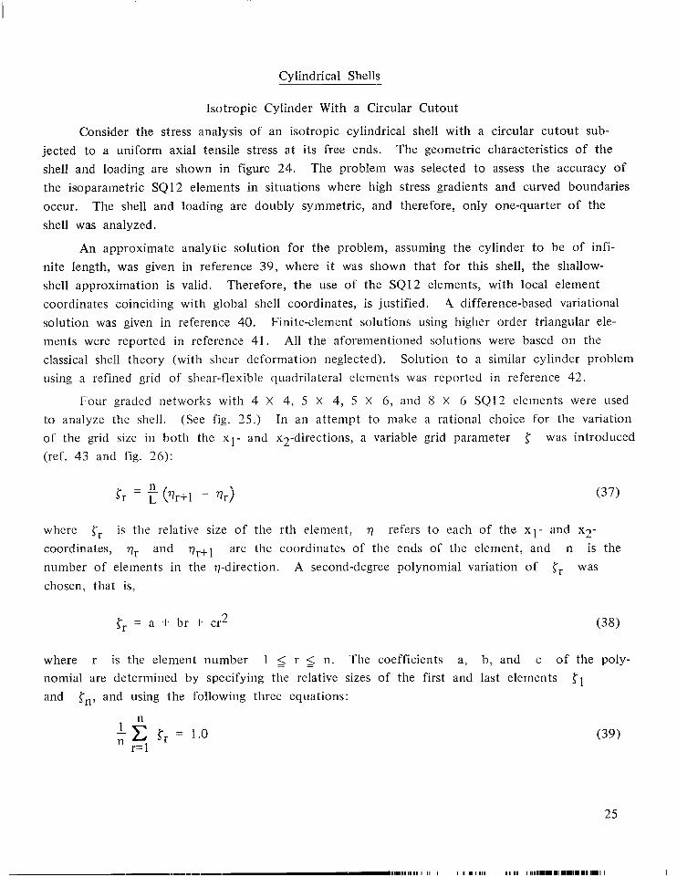
Isotropic Cylinder With a Circular Cutout

Consider the stress analysis of an isotropic cylindrical shell with a circular cutout sub- The geometric characteristics of the jected to a uniform axial tensile stress at its free ends.

shell and loading are shown in figure 24. The problem was selected to assess the accuracy of the isoparametric SQ 12 elements in situations where high stress gradients and curved boundaries occur. shell was analyzed.

The shell and loading are doubly symmetric, and therefore, only one-quarter of the

An approximate analytic solution for the problem, assuming the cylinder to be of infi- nite length, was given in reference 39, where it was shown that for this shell, the sliallow- shell approximation is valid. Therefore, the use of the SQ12 elements, with local element coordinates coinciding with global shell coordinates, is justified. solution was given in reference 40. ments were reported in reference 41. classical shell theory (with shear deformation neglected). Solution to a similar cylinder problem using a refined grid of shear-flexible quadrilateral elements was reported in reference 42.

4 difference-based variational Finite-element solutions using higher order triangular ele-

All the aforementioned solutions were based on the

Four graded networks with 4 X 4, 5 X 4, 5 X 6, and 8 X 6 SQ12 elements were used to analyze the shell. (See fig. 25.) In an attempt to make a rational choice for the variation of the grid size in both the X I - and x2-directions, a variable grid parameter was introduced (ref. 43 and fig. 26):

{

where cr is the relative size of the rth element, 77 refers t o each of the X I - and x2- coordinates, q. and vr+l are the coordinates of the ends of the element, and n is the number of elements in the 77-direction. A second-degree polynomial variation of Cr was chosen, that is,

Cr = a + br + cr2 (38)

where r is the element number 1 5 r 5 n. The coefficients a, b, and c of the polynomial are determined by specifying the relative sizes of the first and last elements and

c l Cn, and using the following three equations:

n

r= 1 1 n - c Cr = 1.0 (39)

25

--..----- 111111111 I1 111 I I I I I I I 1 I 111 I I 111 I 1111111.11 111 1111.111 1111 I I I

{ 1 = a + b + c

The characteristics of the grids used in the present study are shown in figure 26.

The maximum stress concentrations 01 1/u0 grids are given in table 13 along with results of previous investigators. tributions obtained by the 4 X 4 and 8 X 6 grids are shown in figure 27. The high accuracy and rapid convergence of the solutions obtained by the isoparametric SQ12 elements are clearly demonstrated by this example.

and strain energies obtained by the four Membrane stress dis-

Orthotropic Cylinders

The natural frequencies and mode shapes of orthotropic, two-layered, simply supported circular cylinders without axial restraint are studied. The problems are selected to assess the accuracy of the SQH elements when applied t o laminated closed cylinders with high bending- extensional coupling. Shells with fiber orientation (9010) are analyzed.

The geometric characteristics of the shells studied are shown in figure 28.

For these cylinders an analytic solution is obtained and is used as a basis for comparison of the finite-element solutions. It is found that for this shell, the shallow-shell (Donnell’s) theory approximation is valid. The doubly symmetric vibration modes of the cylinders are analyzed and the symmetric boundary conditions along three of the edges are applied. eliminates the axial rigid body mode of the cylinder and allows obtaining the vibration modes having odd values of m (axial direction) and even values of n (circumferential direction). InitialIy a uniform grid with 2 X 2 SQH elements was used to model one octant of the cylinder (grid 1, fig. 29); however, this resulted in poor accuracy for the frequencies and mode shapes with n 2 - 4. Subsequently, the 2 X 2 grid was modified to cover only one-eighth of the circumference (grid 2, fig. 29). This resulted in considerable improvement in the accuracy of the frequencies for The frequencies obtained by the two grids are given in table 14 along with the analytic solutions obtained by both the shear-deformation and classical shallow- shell theories. increases in the circumferential direction, as indicated by the increase of Numerically, the error increases from less than 0.5 percent for m = 1 , n = 2 to approximately 25 percent for m = 1, n = 4. The increased stiffness of the finite-element model due to the larger element size-to-wavelength ratio has caused a greater increase in the error of the finite-element analysis between the two modes. very accurate frequencies provided the element size is less than half the wavelength of the vibration mode.

This

n = 4.

This table shows the decrease in accuracy as the element size-to-wavelength ratio n.

The present example shows that the SQH elements lead to

26

Anisotropic Cylinders

As a final example, consider the free-vibration analysis of anisotropic two-layered circular cylinders. cussed in the preceding subsection, except for the fiber orientation, which is chosen to be

The shells have the same characteristics as those for the orthotropic cylinders dis-

(45/-45).

Solutions are obtained using three grids with 2 X 4, 4 X 8, and 6 X 12 SQH elements (See fig. 30.) In order to eliminate the axial rigid body mode of the in the whole cylinder.

cylinder, u1 and associated mode shapes are shown in figure 31. obtained by the SQH elements is clearly demonstrated by this example.

is set equal to zero a t the center of each grid. The fundamental frequency The rapid convergence of the solutions

CONCLUDING REMARKS

Several shear-flexible finite-element models are applied to the linear static, stability, and vibration problems of plates and shells. The study is based on the shallow-shell theory with effects of shear deformation, anisotropic material behavior, and bending-extensional coupling included. Both stiffness (displacement) and mixed finite-element models are considered. All the elements examined are conforming, satisfactorily represent the rigid body modes, and exhibit uniform convergence for stress-analysis, free-vibration, and buckling problems. Primary attention in t h s study is given to the effects of shear deformation and anisotropic material behavior on the accuracy and convergence of different finite-element models.

On the basis of the present study, the following conclusions seem t o be justified:

1. Higher order displacement models (with cubic or bicubic interpolation polynomials) have the following advantages over lower order models:

(a) The total number of unknowns required for a prescribed level of accuracy is less in the higher order than in the lower order models. This is particularly true for stress resultants and for thinner plates (with negligible shear deformation).

(b) The performance of the higher order models is considerably less sensitive to variations in the thickness ratio and shear deformation than that of the lower order models.

2. The use of derivatives of displacements as nodal parameters (SQH element) has the obvious advantage that the stress resultants are defined directly a t the nodes and no averaging is needed. In addition, this results in improving the performance of the element. in the presence of concentrated loads or discontinuities in the geometric or elastic characteristics of the shell, some of the parameters will be discontinuous and a special treatment is needed.

However,

27

3. The addition of internal degrees of freedom (bubble modes) to displacement models results, in most cases, in improving the performance of the element. where the internal degrees of freedom can be eliminated by static condensation techniques, this is an effective way of improving the accuracy of plate and shell elements without affecting the accuracy of the solution. For free-vibration (and buckling) problems, the addition of internal degrees of freedom is less effective than the addition of nodes to the element. exception to this is the case of the eight-node quadrilateral element when applied to the analysis of higher vibration modes. a much more pronounced effect on the accuracy than the addition of nodes.

In stress-analysis problems

An

In this case, addition of internal degrees of freedom has

4. If mixed models are contrasted with displacement models, the following can be noted:

(a) The development of mixed models involves considerably less algebra than the development of displacement models.

(b) The performance of mixed models is, in general, insensitive to variations in the thickness ratio and shear deformation.

(c) Use of lower order interpolation functions (linear or bilinear) leads to a medi- ocre type of performance. using quadratic shape functions.

Considerable improvement in the performance is achieved by

(d) For a given number of degrees of freedom, the higher order displacement models (with cubic or bicubic interpolation polynomials) lead to higher accuracy than the mixed models with quadratic shape functions. The effective use of mixed models requires the development of efficient equation-handling techniques (e.g., based on hypermatrix stor- age schemes).

5. Whereas material anisotropy was shown to have an adverse effect on the performance of different displacement and mixed elements, the bending-extensional coupling does not seem to have any pronounced effect on the accuracy and convergence of these elements.

Langley Research Center National Aeronautics and Space Administration Hampton, Va. 23665 November 10, 1975

28

APPENDIX A

FUNDAMENTAL EQUATIONS OF SHEAR-DEFORMATION SHALLOW-SHELL THEORY ~ _ _ _ _

The fundamental equations of the shallow-shell theory are given in this appendix.

STRAIN-DISPLACEMENT RELATIONSHIPS

The relationships between strain and displacement are

eap = y(aaup 1 + 3~~1,) + kap w

where ea, are the extensional strains of the reference surface of the shell; ~p are the curvature changes and twist; and 2ea3 are the transverse shearing strain components.

CONSTITUTIVE RELATIONS OF THE SHELL

The relations between the stress resultants and strain Components of the shell are

Qa = ca3p3 2Ep3

The inverse relations are given by

- ‘4 - A&P NYP + B@TP Mw

29

APPENDIX A

w=B @YP NrP + GorPrp Mw

The C, F, and D coefficients are shell stiffnesses and the A, B, and G coefficients are shell compliances defined in appendix B.

30

APPENDIX B

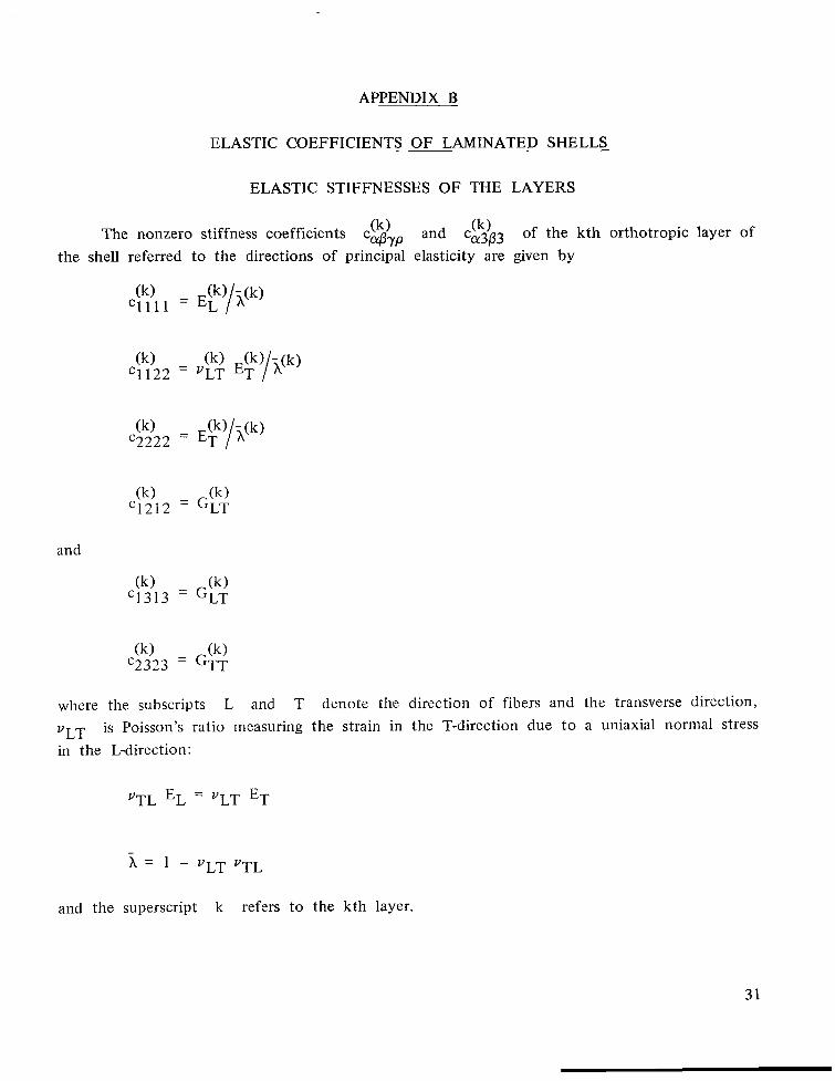
ELASTIC COEFFICIENTS OF LAMINATED SHELLS

ELASTIC STIFFNESSES OF THE LAYERS

(k) The nonzero stiffness coefficients caprp (k) and ca3p3 of the kth orthotropic layer of the shell referred to the directions of principal elasticity are given by

and

where the subscripts L and T denote the direction of fibers and the transverse direction,

VLT is Poisson's ratio measuring the strain in the T-direction due t o a uniaxial normal stress in the L-direction:

"TL E~ = ~ L T ET

and the superscript k refers to the kth layer.

31

APPENDIX B

The stiffness coefficients caprp and ca3p3 satisfy the following symmetry relationships:

If the coordinates x, are rotated, the elastic coefficients caPW and ca3p3 trans- The transformation law form as components of fourth- and second-order tensors, respectively.

of these coefficients is expressed as follows:

Ca‘p‘y’p’ = capyp Qo1,oo Qp,p’ Qy,y‘ Qp,p’

and

where c , ~ p ~ y ~ p ~ and car3pr3 are the stiffness-coefficients referred to the new coordinate system xa‘ and

Q,,,’ = COS( xa,x,’)

ELASTIC COEFFICIENTS OF THE SHELL

The equivalent elastic stiffnesses of the shell are given by

and

k= 1

where NL is the total number of layers of the shell and hk and hk-1 are the distances from the reference surface t o the top and bottom surfaces of the kth layer, respectively. The elastic compliances of the shell B,prp, Gaprp, and Aar3p3 are obtained by inver- sion of the matrix of the elastic stiffnesses. (See ref. 18.)

32

APPENDIX B

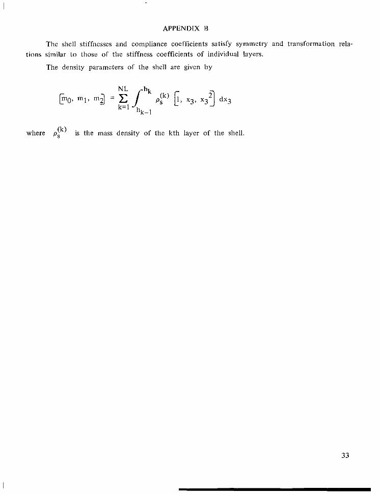
The shell stiffnesses and compliance coefficients satisfy symmetry and transformation relations similar to those of the stiffness coefficients of individual layers.

The density parameters of the shell are given by

where pik) is the mass density of the kth layer of the shell.

33

APPENDIX C

SHAPE FUNCTIONS_U_SED IN PRESENT STUDY

QUADRILATERAL ELEMENTS

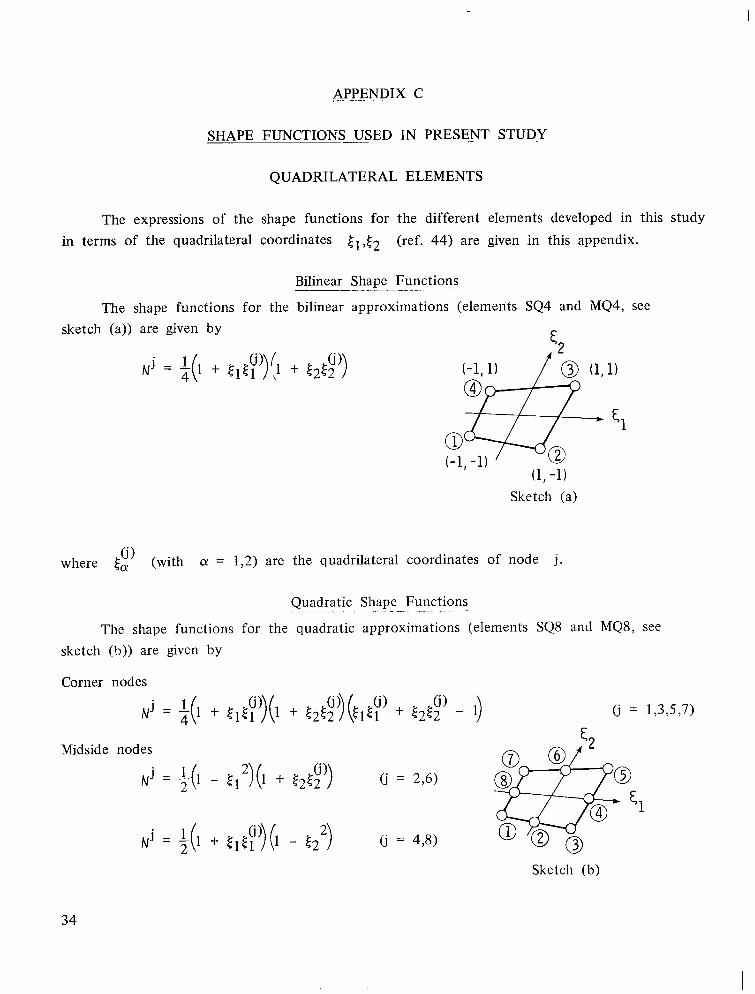
The expressions of the shape functions for the different elements developed in this study in terms of the quadrilateral coordinates (,,E2 (ref. 44) are given in this appendix.

Bilinear Shape Functions

The shape functions for the bilinear approximations (elements SQ4 and MQ4, see __ - -. . - .

sketch (a)) are given by $9

0 (1 , l )

0 (-1, -1)

(1, -1) Sketch (a)

where (with CY = 1,2) are the quadrilateral coordinates of node j .

Quadratic Shape __ _- Functions .

The shape functions for the quadratic approximations (elements SQ8 and MQ8, see sketch (b)) are given by

Corner nodes

Midside nodes

(j = 2,6)

(j = 4,8)

(j = 1,3,5,7) c

Sketch (b)

34

APPENDIX C

Cubic Shape Functions

The shape functions for the cubic approximations (element SQ12, see sketch (c)) are given by

Corner nodes

0' = 1,4,7,10)

$9 Other nodes

Sketch (c)

Hermitian Shape Functions

The Hermitian shape functions (element SQH, sketch (d)) used in products of the following set of first-order Hermite polynomials (sketch

C

Hermitian Shape Functions

The Hermitian shape functions (element SQH, sketch (d)) used in products of the following set of first-order Hermite polynomials (sketch

f1({) = +({3 - 3{ + 2)

f2({) = i ( P 3 - r2 - { + 11

f 3 ( 0 = - l q(C 3 - 3( - 2)

\

0 0

the present (e)):

study were

Sketch (e)

35

APPENDIX C

av av If the order of the nodal parameters at each node is chosen to be v, -- -- * at( at2’

.~

... . j 1 5 9

13

and -__ a”v where v denotes any of the fundamental unknowns, then the shape func- a t 1 at2’

i Q !

~ - ---I-/ 1 3 1 ‘ 3 3 1 3

tions are given by

where the subscripts i and Q are functions of j as follows:

Shape Functions Associated With Nodeless Variables (Bubble Modes) -. - . . . - - . . ~~

Elements SQ5 and SQ9

These elements have one bubble mode given by

/j = 5 for 1

APPENDIX C

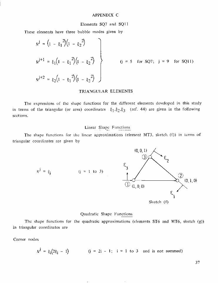
Elements SQ7 and SQ11

These elements have t h e e bubble modes given by

(j = 5 for SQ7; j = 9 for SQ11)

TRIANGULAR ELEMENTS

The expressions of the shape functions for the different elements developed in this study in terms of the triangular (or area) coordinates sections.

E I , E ~ , E ~ (ref. 44) are given in the following

Linear Shape Functions . . . - ~ . _ - -.

The shape functions for the linear approximations (element MT3, sketch (0) in terms of triangular coordinates are given by

(j = 1 to 3)

1 , O )

Sketch (f)

Quadratic Shape Functions

The shape functions for the quadratic approximations (elements ST6 and MT6, sketch (g)) in triangular coordinates are

Corner nodes

Nj = Ei(2Ei - 1) (j = 2i - 1 ; i = 1 to 3 and is not summed)

37

APPENDIX C

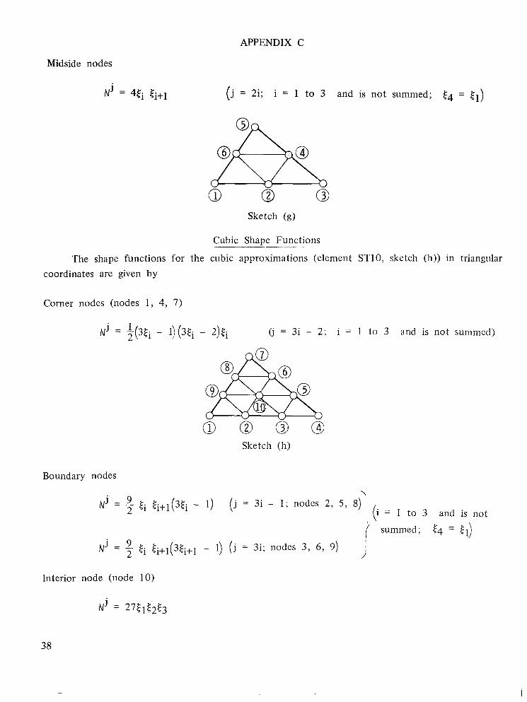
Midside nodes

N~ = 4ti ti+1 (j = 2i; i = 1 to 3 and is not summed; t4 = t l )

Sketch (g)

Cubic Shape Functions .

The shape functions for the cubic approximations (element STlO, sketch (h)) in triangular coordinates are given by

Corner nodes (nodes 1 , 4 , 7)

Sketch (h)

Boundary nodes

\

N j - 9 - - ,ei ,ei+1(3,$i - 1) ( j = 3i - 1; nodes 2, 5 , 8) 2 (i = 1 to 3 and is not

summed; E4 = [I) j - 9 I

j N - 5 ti+1(3ti+] - 1) ( j = 3i; nodes 3, 6, 9)

Interior node (node 10)

38

APPENDIX D

FORMULAS FOR COEFFICIENTS IN GOVERNING

EQUATIONS FOR INDIVIDUAL ELEMENTS

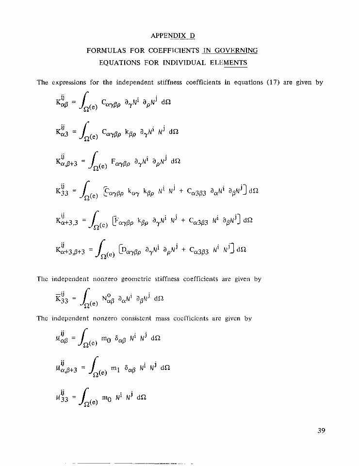
The expressions for the independent stiffness coefficients in equations (17) are given by

The independent nonzero geometric stiffness coefficients are given by

The independent nonzero consistent mass coefficients are given by

39

-- . . , , , ..

APPENDIX D

where 6.p is the Kronecker delta on a and p. The expressions for the “generalized” stiffness coefficients in equations ( 1 8) are given by

Ni N j dS2 ij

sa+6,p+6 = L ( e ) Aa3P3

The consistent nodal load coefficients are given by

P i = Ni N j pj d f l

40

APPENDIX D

In the above equations the contributions of the line integrals have been neglected for simplicity; K is a constant equal to 1 when CY f p and 1/2 when (Y = 0; the range of the lowercase Latin indices is 1 to m, where m is the number of shape functions; the range of the Greek indices is range of the index.

1,2; and a repeated index denotes summation over the full

It should be mentioned that for elements with internal degrees of freedom (SQS, SQ7, SQ9, and S Q l l ) , the indices i j in the expressions for Pk and P; were assumed to have a range equal to the number of nodes in the element (Le., 4 for S Q S and SQ7 elements, and 8 for So9 and SQll elements). of these elements and no loading was associated with internal degrees of freedom.

This means that the loading was distributed on the nodes

41

REFERENCES

1. Whitney, J. M.; and Pagano, N. J.: Shear Deformation in Heterogeneous Anisotropic Plates. Trans. ASME, Ser. E: J. Appl. Mech., vol. 37, no. 4, Dec. 1970, pp. 1031-1036.

2. Srinivas, S.; and Rao, A. K.: Bending, Vibration and Buckling of Simply Supported Thick Orthotropic Rectangular Plates and Laminates. Int. J . Solids & Struct., vol. 6, no. 11, NOV. 1970, pp. 1463-1481.

3. Pagano, N. J.; and Hatfield, Sharon J.: Elastic Behavior of Multilayered Bidirectional Com- posites. AIAA J., vol. 10, no. 7, July 1972, pp. 931-933.

4. Noor, Ahmed K.: Free Vibrations of Multilayered Composite Plates, AIAA J., vol. 11, no. 7, July 1973, pp. 1038-1039.

5. Noor, Ahmed K.; and Rarig, Pamela L.: Three-Dimensional Solutions of Laminated Cylin- ders. Comput. Methods Appl. Mech. & Eng., vol. 3, no. 3, May 1974, pp. 319-334.

Three-Dimensional Finite-Element Comput. & Struct., vol. 2, nos. 5/6, Dec. 1972,

6. Barker, Richard M.; Lin, Fu-Tien; and Dana, Jon R.: Analysis of Laminated Composites. pp. 10 13-1 029.

7. Mau, S. T.; Tong, P.; and Pian, T. H. H.: Finite Element Solutions for Laminated Thick J. Compos. Mater., vol. 6, Apr. 1972, pp. 304-31 1.

8. Argyris, J . H.; and Scharpf, D. W.:

Plates.

Finite Element Theory of Plates and Shells Including Shear Strain Effects. B. Fraeijs de Veubeke, ed., Univ. de Lilge, 1971, pp. 253-292.

High Speed Computing of Elastic Structures, Volume 61 ,

9. Key, Samuel W.; and Beisinger, Zelma E.: The Analysis of Thin Shells With Transverse Shear Strains by the Finite Element Method. Proceedings of the Second Conference on Matrix Methods in Structural Mechanics, AFFDL-TR-68-150, U.S. Air Force, Dec. 1969, pp. 667-710.

10. Irons, Bruce M.; and Razzaque, Abdur: Introduction of Shear Deformations Into a Thin Plate Displacement Formulation. A I M J., vol. 11, no. 10, Oct. 1973, pp. 1438-1439.

1 1. Narayanaswami, R.: New Triangular and Quadrilateral Plate-Bending Finite Elements. NASA TN D-7407, 1974.

12. Zienkiewicz, 0. C.; Taylor, R. L.; and Too, J. M.: Reduced Integration Technique in General Analysis of Plates and Shells. Apr.-June 1971, pp. 275-290.

Int. J. Numerical Methods Eng., vol. 3, no. 2,

13. Fried, Isaac: Shear in Co and C1 Bending Finite Elements. Int. J. Solids & Struct., vol. 9, no. 4, Apr. 1973, pp. 449-460.

14. Fried, Isaac: Residual Energy Balancing Technique in the Generation of Plate Bending Finite Elements. Comput. & Struct., vol. 4, no. 4, Aug. 1974, pp. 771-778.

42

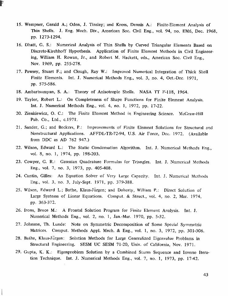
15. Wempner, Gerald A.; Oden, J. Tinsley; and Kross, Dennis A.: Finite-Element Analysis of Thin Shells. J. Eng. Mech. Div., American SOC. Civil Eng., vol. 94, no. EM6, Dec. 1968, pp. 1273-1 294.

16. Dhatt, G . S.: Numerical Analysis of Thin Shells by Curved Triangular Elements Based on Discrete-Kirchhoff Hypothesis. ing, William H. Rowan, Jr., and Robert M. Hackett, eds., American SOC. Civil Eng.,

Application of Finite Element Methods in Civil Engineer-

NOV. 1969, pp. 255-278.

17. Pawsey, Stuart F.; and Clough, Ray W.: Improved Numerical Integration of Thick Shell Finite Elements. Int. J. Numerical Methods Eng., vol. 3, no. 4, 0ct.-Dec. 1971, pp. 575-586.

18. Ambartsumyan, S. A.: Theory of Anisotropic Shells. NASA TT F-118, 1964.

19. Taylor, Robert L.: On Completeness of Shape Functions for Finite Element Analysis. Int. J . Numerical Methods Eng., vol. 4, no. 1, 1972, pp. 17-22.

20. Zienkiewicz, 0. C.: The Finite Element Method in Engineering Science. McGraw-Hill Pub. Co., Ltd., c.1971'.

21. Sander, G.; and Beckers, P.: Improvements of Finite Element Solutions for Structural and Nonstructural Applications. AFFDL-TR-72-94, U.S. Air Force, Dec. 1972. (Available from DDC as AD 762 947.)

22. Wilson, Edward L.: The Static Condensation Algorithm. Int. J . Numerical Methods Eng., vol. 8 , no. 1, 1974, pp. 198-203.

23. Cowper, G. R.: Gaussian Quadrature Formulas for Triangles. Int. J . Numerical Methods Eng., vol. 7, no. 3, 1973, pp. 405-408.

24. Cantin, Gilles: An Equation Solver of Very Large Capacity. Int. J . Numerical Methods Eng., vol. 3, no. 3, July-Sept. 1971, pp. 379-388.

25. Wilson, Edward L.; Bathe, Klaus-Jurgen; and Doherty, William P.: Direct Solution of Comput. & Struct., vol. 4, no. 2, Mar. 1974, Large Systems of Linear Equations.

pp. 363-372.

26. Irons, Bruce M.: A Frontal Solution Program for Finite Element Analysis. Int. J. Numerical Methods Eng., vol. 2, no. 1, Jan.-Mar. 1970, pp. 5-32.

Note on Symmetric Decomposition of Some Special Symmetric 27. Johnson, Th. Lunde: Matrices. Comput. Methods Appl. Mech. & Eng., vol. 1, no. 3, 1972, pp. 301-306.

28. Bathe, Klaus-Jurgen: Solution Methods for Large Generalized Eigenvalue Problems in Structural Engineering. SESM UC SESM 71-20, Univ. of California, Nov. 1971.

29. Gupta, K. K.: Eigenproblem Solution by a Combined Sturm Sequence and Inverse Itera- tion Technique. Int. J. Numerical Methods Eng., vol. 7, no. 1, 1973, pp. 1742 .

43

30. Anderson, M. S.; Fulton, R. E.; Heard, W. L., Jr.; and Walz, J . E.: Stress, Buckling, and Vibration Analysis of Shells of Revolution. Comput. & Struct., vol. 1, nos. 1/2, Aug. 1971, pp. 157-192.

31. Argyris, J. H.; and Willam, K. J.: Some Considerations for the Evaluation of Finite Ele- ment Models. Nucl. Eng. & Des., vol. 28, no. I , 1974, pp. 76-96.

32. Oden, J . T.; and Brauchli, H. J.: On the Calculation of Consistent Stress Distributions in Finite Element Approximations. Int. J. Numerical Methods Eng., vol. 6, 197 1, pp. 317-325.

33. Wilson, E. L.; Taylor, R. L.; Doherty, W.; and Ghaboussi, J.: Incompatible Displacement Models. Nicholas Perrone, Arthur R. Robinson, and William C. Schnobrich, eds., Academic Press, Inc., 1973, pp. 43-57.

Numerical and Computer Methods in Structural Mechanics, Steven J. Fenves,

34. Bell, Kalbein: On the Quintic Triangular Plate Bending Element. Div. Struct. Mech., Norwegian Inst. Technol., Univ. of Trondheim, Norway, June 1972.

35. Chamis, Christos C.: Buckling of Anisotropic Composite Plates. J. Struct. Div., American SOC. Civil Eng., vol. 95, no. STlO, Oct. 1969, pp. 21 19-2139.

36. Morley, L. S. D.: Skew Plates and Structures. Macmillan Co., 1963.

37. Williams, M. L. : Surface Stress Singularities Resulting From Various Boundary Conditions in Angular Corners of Plates Under Bending. GALCIT Publ. No. 330, [ 19541. (Re- printed from ASME Proceedings of the First National Congress of Applied Mechanics.)

Application of Reissner’s Variational 38. Plass, H. J., Jr.; Gaines, J. H.; and Newsom, C. D.: Principle to Cantilever Plate Deflection and Vibration Problems. vol. 29, Mar. 1962, pp. 127-135.

J. Appl. Mech.,

39. Eringen, A. C.; Naghdi, A. K.; and Thiel, C. C.: State of Stress in a Circular Cylindrical Tech. Rep. No. 3-6 (Contract NObs-78866), General Tech- Shell With a Circular Hole.

nology Corp., Aug. 1964.

40. Johnson, Donald E.: A Difference-Based Variational Method for Shells. Int. J. Solids & Struct., vol. 6, no. 6, June 1970, pp. 699-724.

41. Lindberg, Garry M.; and Olson, Mervyn D.: A High-Precision Triangular Cylindrical Shell Finite Element. AIAA J., vol. 9, no. 3, Mar. 1971, pp. 530-532.

42. Key, Samuel W.: The Analysis of Thin Shells With a Doubly Curved Arbitrary Quadrilat- eral Finite Element. Comput. & Struct., vol. 2, no. 4, Sept. 1972, pp. 637-673.

43. Noor, A. K.; and Khandelwal, V. K.: Improved Finite-Difference Variant for the Bending UNICIV Rep. No. R-58, Univ. of New South Analysis of Arbitrary Cylindrical Shells.

Wales, Dec. 1969.

44

44. Desai, Chandrakant S.; and Abel, John F.: Introduction to the Finite Element Method. Van Nostrand Reinhold Co., c. 1972.

45

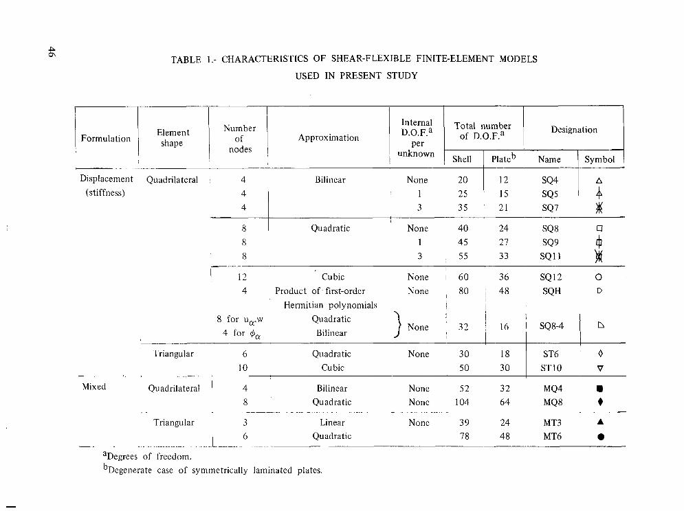
P m

Internal

Per unknown

D.O.F.a Number of

nodes Approximation Element

shape Formulation

I

TABLE 1 .- CHARACTERISTICS OF SHEAR-FLEXIBLE FINITE-ELEMENT MODELS

USED IN PRESENT STUDY

Designation Total number of D.o.F.~

Shell Plateb Name -

Displacement Quadrilateral 4 Bilinear None 20 1 25

4 3 ' 35 (stiffness)

Symbol

12 SQ4 15 SQ5 21 SQ7

I

8 1 Quadratic None 40 24 SQ8 0

8 1 45 27 SQ9 4 8 3 55 33 SQ11 b#

I 12 Cubic None I 60 36 SQ12 0 4 Product of first-order None , SQH D

8o ~ 48 Hermitian polynomials ! I

Triangular 6 Quadratic None 30 18 ST6 ' 0 10 Cubic 5 0 30 I STlO V

- . L - . ~ _ _ _ -

4 Bilinear None 5 2 32 MQ4 a + 8 Quadratic None 104 64 MQ8

Triangular 3 Linear None 39 24 MT3 A 6 Quadratic 78 48 MT6 0

c

Mixed Quadrilateral I , . _ - .... . . . . . . . . + ................ . . . . -

-. ..... . . .__I . .

"Degrees of freedom. bDegenerate case of symmetrically laminated plates.

TABLE 2.- BOUNDARY CONDITIONS USED IN PRESENT STUDY

@ denotes suppressed degree of freedom; 1 , free (unrestrained]

U 3-a 0

0

1

Boundary xa = Const

' Simple support

Clamped I I Line of symmetry

@a 0 1 0

0 0 0

1 0 1

-- (b) Force boundary conditions Boundary xa = Const %,a N 3-a,3-a N12 Ma,, M3-a, 3-a

K~ = 1 for anisotropic shells and 0 for isotropic or orthotropic shells. a

Clamped 1 1 1

Free 0 1 0

Line of symmetry 1 1 0

M12 Qa Q3-a

1 1

0 1

1 1

1 1 1 a K a ,

1 1

0 0

0 0

a Ka

1

1

P 00

TABLE 2.- Concluded

(c) Boundary conditions for SQH element along edge x, = Const I I i

fsplacement

I ucY

W !

Simple support Clamped Line of symmetry I I

0 1

1

t I

1

f a a,f a3-af 1 bK 1

0 1 0 1 1 0 : 1 0

' 1 ' 0 0 1 1 I

0 1 I

a f stands for any of the generalized displacements b -

ucY, w, $u K - 0 if force boundary conditions are imposed and 1 otherwise.

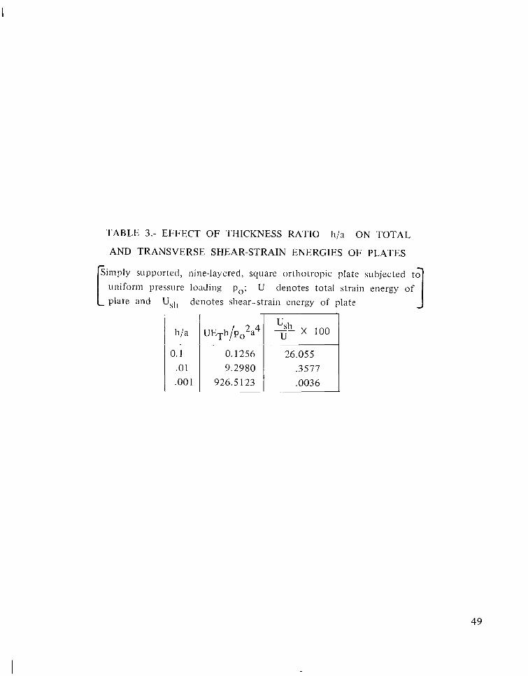
TABLE 3.- EFFECT OF THICKNESS RATIO 11/a ON TOTAL

AND TRANSVERSE SHEAR-STRAIN ENERGIES OF PLATES

supported, nine-layered, square orthotropic plate subjected to 3 uniform pressure loading p,; U denotes total strain energy of plate and Usll denotes shear.-strain energy of plate

h/a

0.1 .01 .oo 1

0.1256 26.055 9.2980 .3577

926.5 123

49

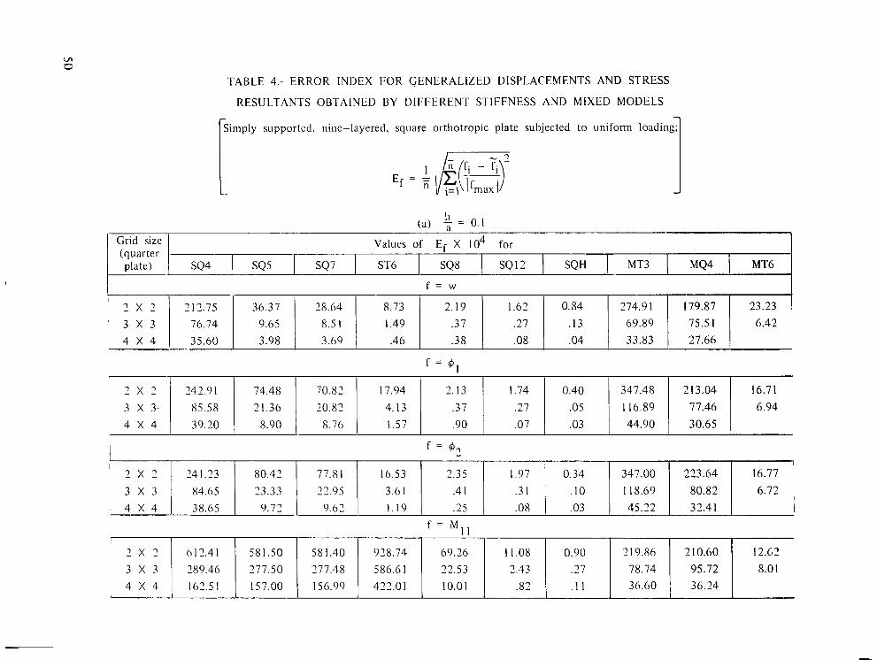
TABLE 4.- ERROR INDEX FOR GENERALlZED DISPLACEMENTS AND STRESS

RESULTANTS OBTAINED BY DlFFERE,NT STIFFNESS AND MIXED MODELS

supported, nine-layered. square orthotropic plate subjected to unifonn loading; 1

2 x 3 2 12.75 , 3 x 3 76.74

4 x 4 35.60

I

36.37 28.64 8.73 2.19 1.62 0.84 274.9 1 179.87 23.23 9.65 8.5 1 1.49 .37 .27 .13 69.89 75.5 1 6.42 3.98 3.69 .46 .38 .08 .04 33.83 27.66

I1 ( a ) ;1 = 0.1

I Grid size I Values of E~ x 104 for

2 X 2 242.91 74.48 70.81 17.94 2. I3

3 x 3- 85.58 21.36 30.81 4.13 .37 4 x 4 39.20 8.90 8.76 I .57 .90

1.74 0.40 347.45 2 13.04 16.7 1 .27 .05 116.89 77.46 6.94 .07 .03 44.90 30.65

I 2 x 3 3 x 3 4 x 4

1

741.23 80.42 77.81 16.53 3.35 1.97 0.34 347.00 223.64 16.77

84.05 23.33 33.95 3.6 1 .4 1 .3 1 .10 118.69 80.82 6.72

38.05 9.72 9.63 1.19 .25 .08 .03 45.22 32.4 1 1

I

2. X 2 3 x 3 4 x 4 - -J

12.62 78.74 95.72

612.41 58 1 S O 58 1.40 928.74 69.36 11.08 289.46 277.50 277.48 586.6 1 22.53 2.43 .27 162.5 I 157.00 156.99 422.0 1 10.0 1 .82 36.60 36.24

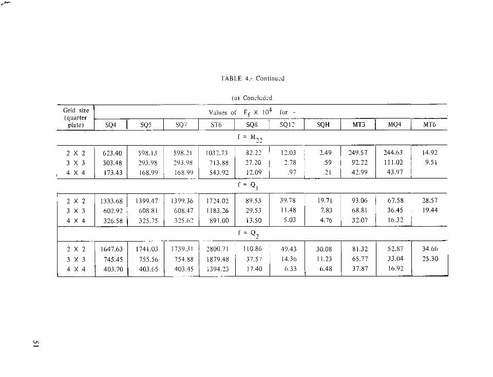
TABLE 4.- Continued

( a ) ConclLlded

Grid size (quarter

plate)

values of E~ x 104 for - - SQ4 I SQS I SQ7 I ST6 I SQ8 I SQI2 SQH 1 MT3 MQ4 1 MT6

2 x 2 3 x 3

, 4 x 4

623.40 598.13 598.21 1032.73 82.22 ' 12.03 2.49 249.57 244.63 14.92 303.48 293.98 293.98 713.88 27.20 I 2.78 .59 92.22 1 1 1.02 9.5 1 173.43 168.99 168.99 543.92 12.09 1 .97 .21 42.99 43.97

2 X 2 1333.68 1399.47 1399.36 1724.02 89.53 39.78 19.71 93.06

3 x 3 602.92 608.8 1 608.47 1 183.26 29.53 11.48 7.83 68.81

4 x 4 326.58 325.75 325.62 891.00 13.50 5.03 4.76 32.07

67.58 28.57 36.45 19.44 16.32

2 X 2

3 x 3 4 x 4

1647.63 1741.03 1739.31 2800.71 110.86 ' 49.43 30.08 81.32 52.87 34.66 745.45 755.56 754.88 1879.48 37.57 14.36 11.23 65.77 33.04 25.30 403.70 403.65 403.45 1394.23 17.40 6.33 6.48 37.87 16.92

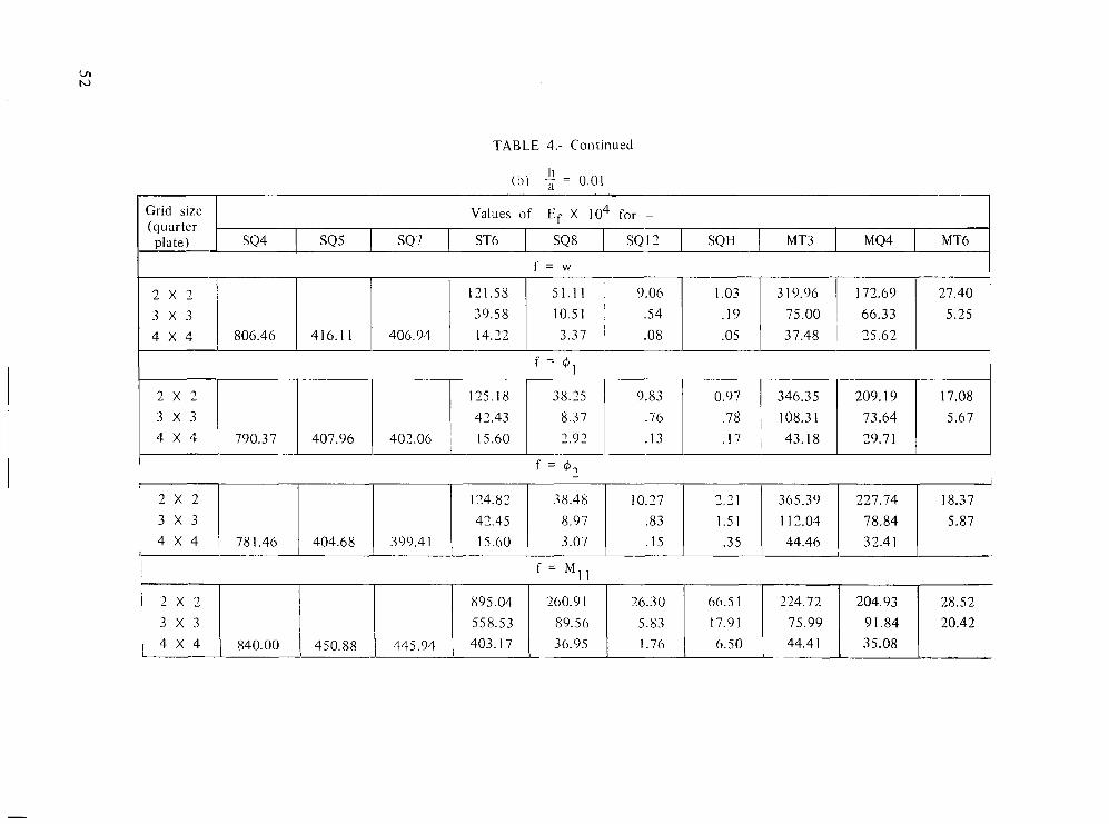
TABLE 4.- Continued

I1 (11) 3 = 0.01

2 x 2 121.58 51.11 9.06 1.03 3 x 3 39.58 10.5 1 .54 . I9 4 x 4 806.46 416.1 1 406.94 14.22 3.37 .08 .os

-

Values of E~ x 104 for -

3 19.96 172.69 27.40 75.00 66.33 5.25 37.48 25.62

2 x 2 3 x 3 4 x 4 790.37 407.96

1 f = $

125.18 38.25 9.83 0.97 346.35 209.19 17.08 42.43 8.37 .76 .78 108.3 1 73.64 5.67

403.06 15.60 2.92 . I 3 . I 7 43.18 29.7 1

134.82

4 x 4 15.60

38.48 10.27 2.2 1 365.39 227.74 18.37 8.97 .83 1.51 112.04 78.84 5.87 3.07 .15 .35 44.46 32.41

345.94

895.04 260.9 1 36.30 66.5 1 324.72 204.93 28.52 558.53 89.50 5.83 17.91 75.99 91.84 20.42

30.95 I .70 0.50 44.4 1 35.08 -

403.17

1 2 x 2 3 x 3

1 4 X 4 840.00 I 450.88

Grid size ( q liar ter

plate)

values of ~f x 104 for

SQ4 SQ5 SQ 7 ST6 SQ8 SQI2 SQH MT3 MQ4 MT6

2 x 2 965.51 309.37 37.40 76.21 279.10 258.03 089.66 1 17.78 9.40 22.58 99.72 114.38

4 x 4 859.45 462.04 457.63 531.80 52.16 3.00 8.83 52.92 46.04

33.35 26.88

2 x 2 106803.72 3674.66 , 1812.85 838.56 100.53 57.10 3 x 3 77899.77 1514.77 329.35 227.36 80.35 37.56 4 X 4 4989.61 14280.28 14775.74 60490.19 853.06 91.98 84.28 49.39 16.93

60.86 62.63

180688.96 4254.03 1306.80 1387.85 97.70 27.27 178160.13 1638.37 431.93 390.99 94.43 38.84

130.24 148.15 59.50 19.4 1

68.30 78.48

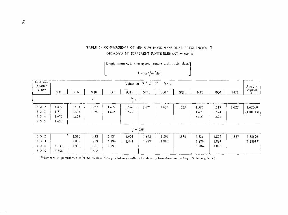
TABLE 5.- CONVERGENCE OF MINIMUM NONDIMENSIONAL FREQUENCIES X OBTAINED BY DIFFERENT FINITE-ELEMENT MODELS

Grid size (quarter

plate)

supported, nine-layered, square orthotropic plate; 1 Values of X: x 10-l for -

Analytic s o h tion

SQ4 I ST6 I SQ8 1 SQ9 SQI I STlO SQ12 ! SQH I MT3 I MQ4 I MT6 (a)

1

2 x 2 ~ 3 x 3

4 x 4 5 x 5

J

1.827 1.633 1.627 1.627 1.626 1.625 1.625 1.625 1.587 1.619 1.625 1.62500 1.714 1.627 1.675 1.625 1.625 1.620 1.624 (1.88913) 1 1.675 1.626 1.623 1.625 I .657

2 x 2 3 x 3 4 x 4 5 x 5

I

'Numbers i n parentheses refer to classical-theory solutions (with both shear deformation and rotary inertia neglected).

2.010 1.932 1.921 1.905 1.892 I .896 1.886 1.836 I .877 1.887 1.88576 1.939 1.899 1.898 1.891 1.887 1.887 1.879 1.884 (1.88913)

4.131 1.910 1.891 I .89 I 1.884 1.885 3.558 I .888 UL

TABLE 6.- CONVERGENCE OF NONDIMENSIONAL FREQUENCIES Xm,n OBTAINED BY DIFFERENT STIFFNESS MODELS

Simply supported, nine-layered, square orthotropic plate; r -

(quarter plate)

h (a) a = 0.1

soultion '

SQH (a) SQ4 ST6 SQ8 SQ9 SQ11 STlO SQ12

Grid .

size

8.111 6.100 i 6.094 6.088 ' 5.971 6.989 5.972 5.959 5.959 ' 5.931 6.519 5.934 j

Values of Xm,-, for -

5.937 5.933 5.930 5.92149 5.923 5.922 (10.500)

Analytic

2 x 2 8.191 1 6.404 i 6.393 6.388 6.280 6.249 6.245 6.242 3 x 3 7.208 6.281 , I 6.269 6.267 6.242 6.235 6.235 4 x 4 6.78 1 6.250 6.345 6.245

6.23387 (12.9354)

2 x 2 3 x 3 4 x 4

2 x 2 3 x 3 4 x 4

~

8.466 19 8.517 8.484 8.479 8.488 ( 17.0022)

11.380 9.197 9.052 8.694 8.559 8.595 8.768 8.478 9.901 8.710 8.542

8.558 8.487 8.483

aNumbers in parentheses refer to classical-theory solutions (with both shear deformation and rotary inertia neglected).

TABLE 6.- Concluded

(1.)) ; = 0.0 1

ST6 SQ8

Values of Xm,* for -

SQH , (a) SQ9 SQ11 STlO SQ12

I I Analytic

1.324 1.278 1.150 1.1 12

4 x 4 2.885 1.087 1.070

1.239 1.110 1.072 1.042 (1.0500) 1.070

1.638 1.383

4 x 4 2.985 1.318 ..

1.530 1.499 1.390 1.303 1.305 1.292 1.2720 1 ' 1.349 1.347 1.303 1.276 1.275 (1.29354) 1.303 1.303

aNumbers in parentheses refer to classical- theory solutions (with both shear deformation and rotary inertia neglected).

4.146

2.942 3.856 1.975 1.825 1.902 2.297 1.703 1.67351 2.242 1.926 1.775 1.718 1.709 1.782 (1.70022) 1.935 1.734 1.716

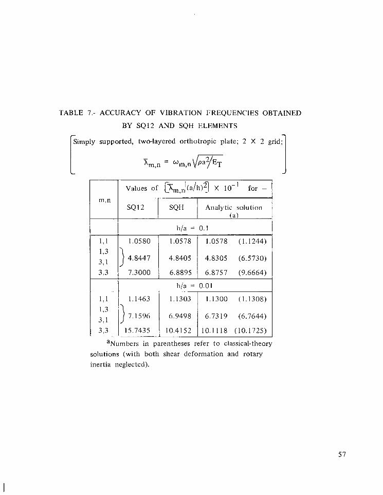
TABLE 7.- ACCURACY OF VIBRATION FREQUENCIES OBTAINED

BY SQ12 AND SQH ELEMENTS

1 7 1 1’3 321 373

supported, two-layered orthotropic plate; 2 X 2 grid; 1

1 .OS80 1.0.578 1.0578 (1.1244)

} 4.8447 4.8405 4.8305 (6.5730)

7.3000 6.8895 6.8757 (9.6664)

h/a = 0.01

c

1,1 1’3 3,1

Analytic solution

h/a = 0.1

1.1463 1.1303 1.1300 (1.1308)

6.9498 6.73 19 (6.7644) } 7.1596

3,3 I 15.7435 1 10.4152 I 10.1118 (10.1725) 1 aNumbers in parentheses refer to classical-theory

~~

solutions (with both shear deformation and rotary inertia neglected).

57

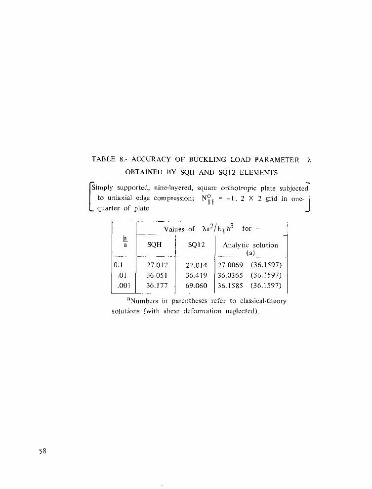
TABLE 8.- ACCURACY OF BUCKLING LOAD PARAMETER h

OBTAINED BY SQH AND SQ12 ELEMENTS

supported, nine-layered, square orthotropic plate subjected 1 to uniaxial edge compression; quarter of plate

NY1 = - 1 ; 2 X 2 grid in one-

s Q ~ a l u e s c 4 a 2 [ E ~ h 3 for - - Analytic solution

_ _ _ _ ~ ~ (a) -. 27.012 27.014 27.0069 (36.1597) 36.05 1 36.4 19 36.0365 (36.1597)

.001 36.177 69.060 36.1585 (36.1597)

58

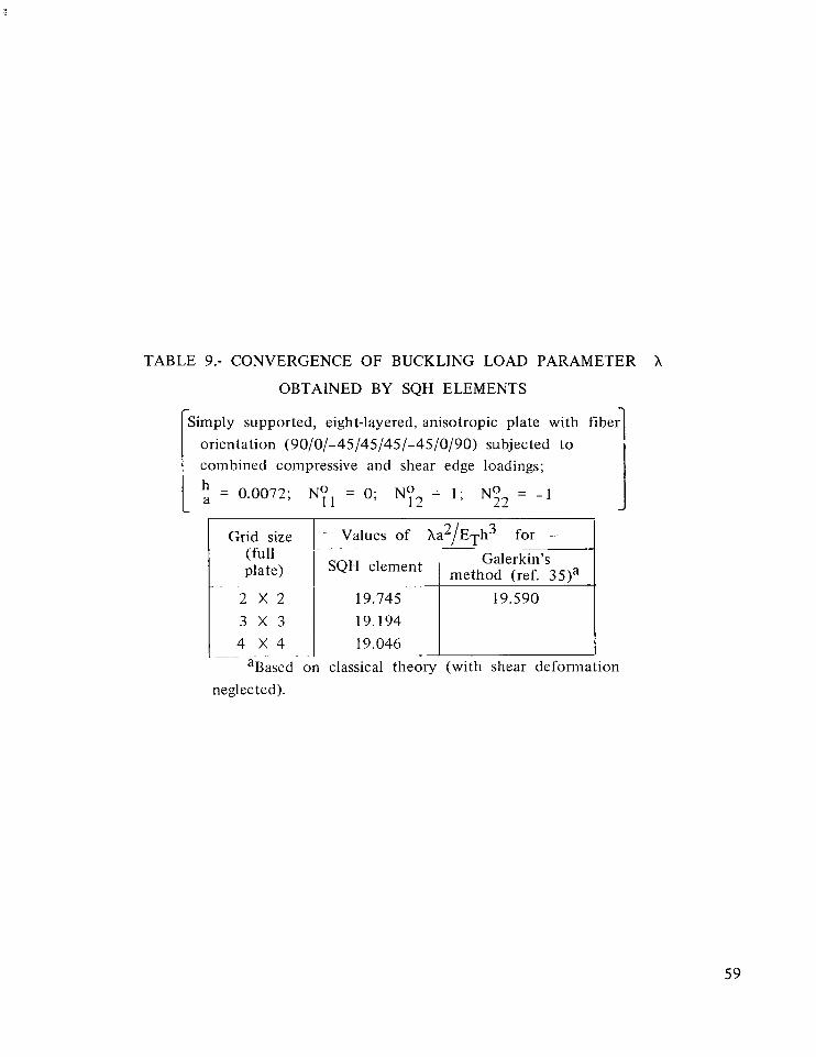
TABLE 9.- CONVERGENCE OF BUCKLING LOAD PARAMETER h

Grid size L Values Of h a 2 / E ~ h 3 for - I saH Galerkin’s plate) method (ref. 35)a

. .. - - . .

2 x 2 19.745 19.590 3 x 3 19.194 4 x 4 19.046

OBTAINED BY SQH ELEMENTS

[Simply supported, eight-layered, anisotropic plate with fiber 1 I orientation (90/0/-45/45/45/-45/0/90) subjected to 1 combined compressive and shear edge loadings;

!-- - . 1 I

aBased on classical theory (with shear deformation neglected).

59

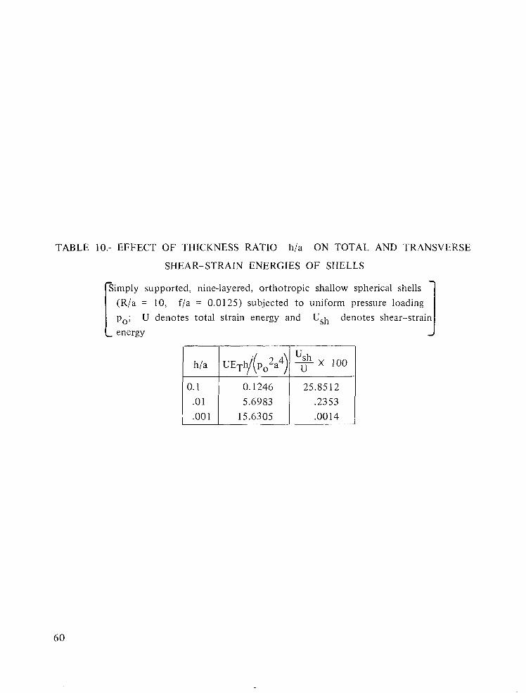
TABLE 10.- EFFECT OF THICKNESS RATIO li/a ON TOTAL AND TRANSVERSE

SHEAR-STRAIN ENERGIES OF SHELLS

po; U denotes total strain energy and Ush denotes shear-strain (R/a = 10, f/a = 0.0125) subjected to uniform pressure loading 1 supported, nine-layered, orthotropic shallow spherical shells

0.1246 25.85 12 .2353 .0014

- - - .oo 1 15.6305

60

TABLE 1 1 .- CONVERGENCE OF NONDIMENSIONAL FREQUENCIES xnl,,, OBTAINED BY DIFFERENT STIFFNESS MODELS

supported, nine-layered, orthotropic shallow 1 R f spherical shell ( 2- = I O . ;1 = 0.0125);

(qiiarter SQ9 SQI 1 STI 0 5q12 SQH

Grid ~ size 1

solution '

(a)

Values of XI,,,, X 10 for

2 x 2

3 x 3 4 x 4

Analytic

1.039 1.633 1.632 1.631 1.63 1 1.63 1 1.630 1.630

1.632 1.63 I 1.63 1

1.630 ( 1.893)

2 x 2

3 x 3

4 x 4

6. 104 0.00 0 6.09 1 5.913 5.939 5.935 5.932 5.924

5.914 5.00 1 5.96 1 5.930 ( 10.496

2 x 2

3 x 3

4 x 4

1 in = 3. n = 1

6.408 0.3 9 5 6.390 6.281 6.251 6.346 6.744 6.236

0.283 6.21 1 0.270

0.241

2 x 2 0.20 1 9.055 8.695 8.560 8.595 8.770 8.478

3 x 3 8.71 1 8.543 8.518

4 x 4 8.487

8.467

(17.001)

TABLE 11.- Concluded

Grid size

(quarter shell) ST6 SQ8 SQ9 SQ11 STlO 5q12 SQH

Values of Xm,n x 102 for - Analytic solution

(a)

j 2 x 2 1.66 1 1.55 1 1.520 1.409

~ 4 x 4 1.323 3 x 3 1.403 1.368 1.367

0.2538 0.2452 0.2443 0.2428 0.24 17 0.2419 0.24 12 .2459 .2422 .2422

.24 16

1.292

(1.3 13)

0.241 1

(0.2414)

I m = 3 , n = 3

2 x 2 1.350 1.303 1.265 1.182 1.094 1.099 1.084 ~ 3 x 3 1.173 1.136 1.134 1 4 x 4 1.094

1.063

( 1.074)

aNumbers in parentheses refer to classical-theory solution (with shear deformation and rotary inertia neglected).

I

' 2 x 2 2.955 3.862 3 x 3 2.250 1.933 4 x 4 1.741

1.680 1.986 1.833 1.909 2.303 1.709 1.783

TABLE 12.- EIGENVALUES O F THE STIFFNESS MATRICES FOR VARIOUS DISPLACEMENT MODELS

flia = 0.0125: side length of element in coordinate directions orientation ~451-45/45/-45/45/-45/45/-45/45); R/a = I O ; 1 shallow spherical shell with fiber

ST6 SQ8 SQ9 SQ11 STIO SQ12 i SQH

1.132 X 1.251 X 1.338 X 5.165 X

~ P7 4.278 X 5.890 X 5.890 X i 5.183 X

P6 i Straining Bmax 9.389 6.276 1.175 X I O 1 1.175 X I O ’

Trace 2.170 X 10’ 3.010 X 10’ 4.245 X 10’ 5.162 X 10’ i

1.681 X 1.250 X 5.094 X I O - ”

1.549 X 3.969 X 7.870 X

2.047 X I O 1 1.232 X 10’ 2.679

6.522 X 10’ 8.614 X 10’ 1.233 X 10’

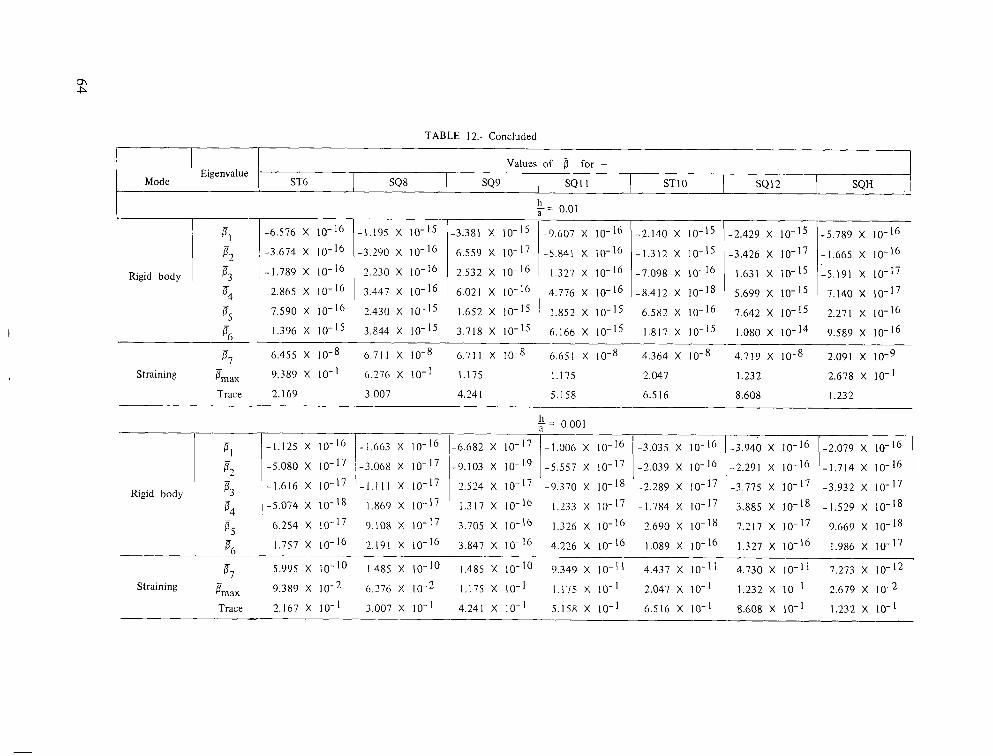
ch P

Eigenvalue Mode

i

Values of for - -

ST6 SQ8 SQ9 SQl I STlO SQl2 SQH ,

-1.195 x 10-15

-3.290 X

2.230 X

3.447 x 10-16 Rigid body

8, 1-6.576 X

/-3,674 X

-1.789 X P; 7.590 X 2.430 X 1 1.652 X ~ 1.852 X 6.582 X 7.642 X

1.396 X IO-" 3.844 X 3.718 X 6.166 X 1.817 X 1.080 X 4

$7

'6

6.455 X 6.711 X 6.711 X 6.651 X 4.364 X 4.719 X

Straining Emax 9.389 X I O - ' 6.276 X 10-1 1.175 1.175 2.047 1.232

Trace 2.169 3.007 4.241 5.158 6.516 8.608

-3.381 X

6.559 X

2.532 X

6.021 X

-5.789 X

-1.665 X

-5.191 x 10-17 7.140 X

2.271 X

9.589 X

-9.607 X

-5.841 X 10-l6

1.327 X

4.776 X

2.091 X

2.678 X I O - 1

1.232

-1.125 x 10-16

E2 -5.080 x 10-17 PI

6.254 x 10-17 E5 P;, 1.757 X

-1.663 X

-3.068 x 10-17 - 1 . 1 1 1 x 10-17 1.869 X

9.108 X

2.191 X

-6.682 X

-9.103 x 10-19 2.524 x 10-17 1.317 X

3.705 X

3.847 X

= 0.001

-1.006 X

-5.557 x 10-17

1.233 x 10-17 -9.370 X

1.326 X

4.226 X

-3.035 X

-2.039 X

-2.289 x 10-17 -1.784 x 10-17 2.690 X

1.089 X

-3.940 X -2.079 X

-2.291 X ,-1.714 X

-3.775 x 10-17 -3.932 x 10-17 3.885 X -1.529 X I O W i 8

7.217 X 9.669 X

1.327 X 1.986 X

5.995 X lo-'' 1.485 X IO-" 1.485 X IO-" 9.349 X 4.437 X I O - ' ' 4.730 X 7.273 X

Straining 9.389 X 6.7-76 X IO-* 1.175 X I O - ' 1.175 X IO- ' 2.047 X I O - ' 1.232 X 10-1 2.679 X E7

Trace 2.167 X I O - ' 3.007 X I O - ' 4.241 X I O - ' 5.158 X I O - ' 6.516 X I O - ' 8.608 X I O - ' 1.232 X 10-1

TABLE 13.- COMPARISON OF SOLUTIONS OBTAINED BY ISOPARAMETRIC SQ12

degrees of freedom

525

640

920

ELEMENTS WITH THOSE OF PREVIOUS INVESTIGATORS

kircular cylindrical shell with a circular cutout loaded in tension 3

Membrane

3.643

3.691

3.7 12

L

Grid

4 x 4

5 x 4

5 x 6

8 x 6

Finite differences (ref. 40)a

Finite elements (ref. 41)a

(ref. 391a Analytic solution

Number of

I

1415 3.666

3.603 753 I

I

3.690

3.658 367 I

1

-

Membrane + bending

4.268

4.252

4.257

4.223

4.096

4.249

bE/(uo2h3d X

(b) - 4.73495 1

4.735373

4.7 1 1623

4.724903

4.729269

4.180 L aBased on the classical theory (with shear deformation neglected). bStrain energy in one-quarter of the shell.

65

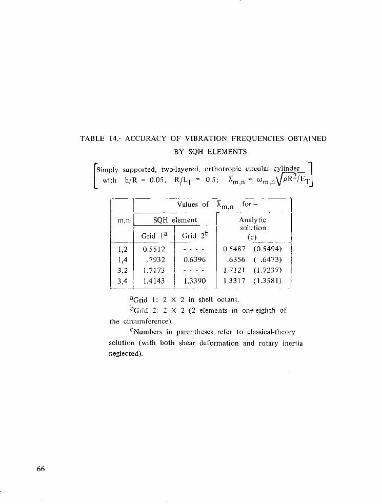
TABLE 14.- ACCURACY OF VIBRATION FREQUENCIES OBTAINED

BY SQH ELEMENTS

Simply supported, two-layered, orthotropic circular - with h/R = 0.05, R/L1 = 0.5; Xm,-, - c

m,n

Values of I SQH element

Grid l a Grid 2b

1,2 0.5512 1,4 .7932 3,2 1.7173 3,4 , 1.4143

I

___ _ _ _ _ _ for -

xm,n .. j Analytic solution

(c) 0.5487 (0.5494)

.6356 ( .6473) 1.7121 (1.7237)

~- I - _ - -

0.6396 - - - -

1.3390 - ..

1 1.3317 (1.3581) .-

aGrid 1: 2 X 2 in shell octant. bGrid 2: 2 X 2 (2 elements in one-eighth of

‘Numbers in parentheses refer to classical-theory the circumference).

solution (with both shear deformation and rotary inertia neglected).

66

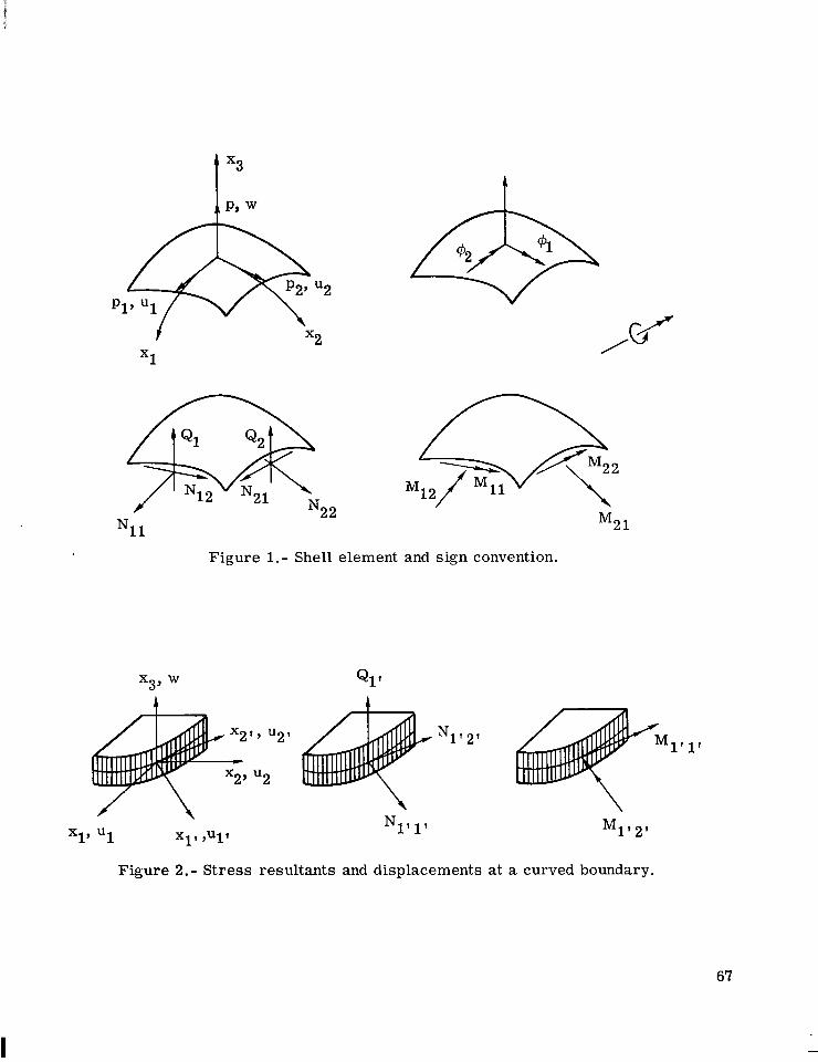
P1' mu2 u1

x1

N1 1 LL

Figure 1. - Shell element and s ign convention.

M 2 1

1' 1' N 1 ' 2 '

xl' u1 XI1 'U l '

F igu re 2.- S t r e s s resul tants and displacements a t a curved boundary.

67

I' --- .......

Figure 3. - Charac ter i s t ics of laminated graphite-epoxy plates used i n present study.

68

Q. A x2 1.20

1.15

1.10

1.05 cd 3

3 > 1.00

.9 5

.90

4 W = 5.848 x 'oa exact MT3 f 3

ETh

\A

.8 5 1 2 3 4 5

Number of elements per side (quarter plate) (a) w at point A.

1.30 -

1.20 I MT3 @2,exact

ST6, STlO I I \

B k--a/2-4 A

a J m

I D

* : 3J.10 N a \ a"

1.00

.90

3 a = 1.533 x P,

ETh3

1 2 3 4 5

Number of elements per side (quarter plate)

(b) q52 at point B.

Figure 4.- Convergence of s t r e s s resultants and generalized displacements with grid refinement. Simply supported, nine-layered, orthotropic square plate with = 0.1.

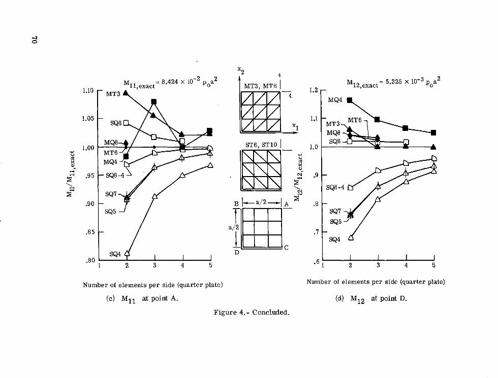
2 X I

1.10

1.05

1.00 U V cd x a!!

‘2l

rl $ .95

x- .90

.85

2 = 8.424 x IO- poa2 M1 I, exact

’ MT3 4

I I I 1 2 3 4 5 .80

e 1 MT3, MT6 I

ST6, STlO I

x B A

2 = 5.325 x p,a M1 2, exact 1.2 r

1.1

1.0

- *6 1 2 3 4 5

Number of elements per side (quarter plate) Number of elements per side (quarter plate)

(c) Mll at point A. (d) M12 at point D.

Figure 4. - Concluded.

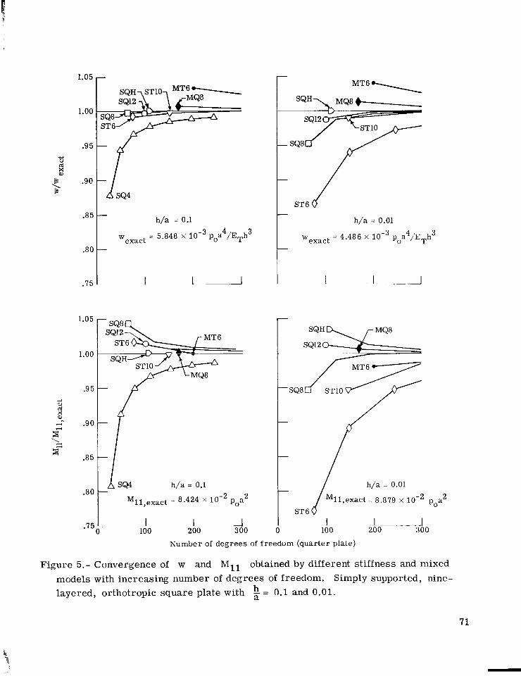
1.05

1.00

.9 5

.9@

.85

.80

.75

1.05

1.00

.9 5

.9 0

.85

.80

.75

f’

- h/a = 0.1

3 4 3 - 5.848 X 10- P0a /ETh exact - W

-

I 1 1

- 4 4

h/a = 0.1

M1l,exact = 8.424 x poa2 -

I , 100 200 300

4 -

ST6 -

h/a = 0.01

Wexact - - 4.486 x poa4/ETh3

I 1 2

h/a = 0.01

M11,exact = 8.879 x 10-2 POa 2 ST 6 u 200 300

- 4 1

100 Number of degrees of freedom (quarter plate)

F igu re 5.- Convergence of w and MI1 obtained by different st iffness and mixed Simply supported, nine- models with increasing number of deg rees of f reedom.

layered, orthotropic squa re plate with : = 0.1 and 0.01.

71

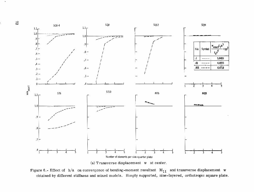
SQ8-4

.6 t

.5 -

.4 - .3 - .2 -

/' .1 - /'

0 . I 1 1 /'

.7 I-

.6 1 I I I I 1 2 3 4 5

.7 '- I

.6 - i i

I

I i .5 -

I

.4 ' I I I J

ST10

I-

I I I I I 1 2 3 4 5

I - I i

I -

I I - ;

c

SQ12

MT6 r

hla Symbol -

-01 I ---- I 4.4855 I

I, I I I I 1 2 3 4 5

I I I I 1 1 2 3 4 5


(a) T r a n s v e r s e displacement w at center.

F igure 6.- Effect of h/a on convergence of bending-moment resultant MI1 and t r ansve r se displacement w obtained by different stiffness and mixed models. Simply supported, nine-layered, orthotropic squa re plate.

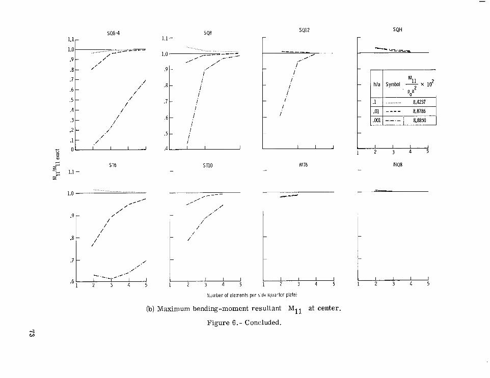
4 w

1.0

.9

.8

.7

SQ8-4 1.1

, , . . . . . .

.................................. .- ,---- .' /'

/ /' /

/- ,' / - /'

/ - / /

/ /

/ /

- /

- / / '

./ ' -.

::I (. ,,; , .3

.2 /.

.1 0

/.

S T6 A

s- s- -- 1.1 -

S Q8 1.1 -

1.0 .. ..... . .........._..,... ....._ ....

0----- ,e.-.- , .' / /'

/'

i i i i i

I

/ .5 .6L .4

5912

I i i i

I I'

-.-.- I 8.8850

I I I I 1 2 3 4 5

MT6 MQ8


(b) Maximum bending-moment resultant Mll at center.

Figure 6.- Concluded.

I I I I 2 3 4 5

1.15

1.12 1 SQ4\ w exact - - 1 . 6 2 5 0 4 3

1.03 1 1 ST61

2 3 . 4 5 .97 1


(a) h - = 0.1. a

1.09 ST6,STlO I

I

1.06

1.03 B I

1.00

.9 7 MT 3 -& 2 3 4 5


(b) $ = 0.01.

Figure 7.- Convergence of fundamental frequency obtained by different st iffness and mixed models with gr id refinement. Simply supported, nine-layered, orthotropic square plate.

m = 1, n = 3

1.4

1.3

1.2

1.1

1.0

.9 4 2 0 Ld x a,

3 3

m = 1, n = 1

2 - w = 1.6250 dl3 d p a exact

""\ SQ5

- . SQ7

1 1 I J

m = 3 , n = l "c 1.3 sQ4\ D 1.2 \ u exact = 6.23394ET/pa2

1.1

1.0 F: I

t

r

I - I I 1

m = 3 , n = 3

I': I

I I I 1 1 3 4 5 1 2 3 4 5

.9 I I ~ 2 1

Number of e l emen t s p e r side (quar te r plate)

(a) = 0.1; four-node quadri la terals .

F igu re 8.- Effect of internal deg rees of f reedom on accuracy and convergence of vibration frequencies. Simply supported, nine-layered, orthotropic s q u a r e plate.

75

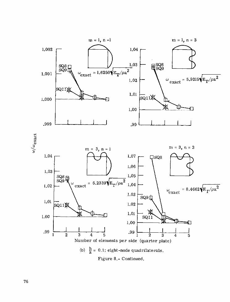
m = 1, n =1 m = 1, n = 3

1.002

1.00 1

1,000

.999

4 0 cd x

\ 3 z?

1.04

1.03

1.02

1.01

1.00

m = 3 , n = l m = 3 , n = 3

1 2 3 4 5 .99

1.04

1.03

1.02

1.01

1.00

I- \ - 2 3 4 5

.99

Number of e lements p e r s ide (qua r t e r plate)

(b) h - = 0.1; eight-node quadri la terals , a Figure 8. - Continued.

76

m = 1. n = 1

I

m = l , n = 3

.9 5

1.04

1.03

1.02

1.01

1.00

I I 1 I I I I .95 1

r 1.25

1.20

= 0 . 1 8 8 5 8 d g 1-15

1.10

1.05

exact

1.00 I U u cd x a

3 3

1.25

1.20

1.15

1.10

1.05

1.00

-

1.05

m = 3 , n = 3

2.3039

W = 1 exact ..6736

77

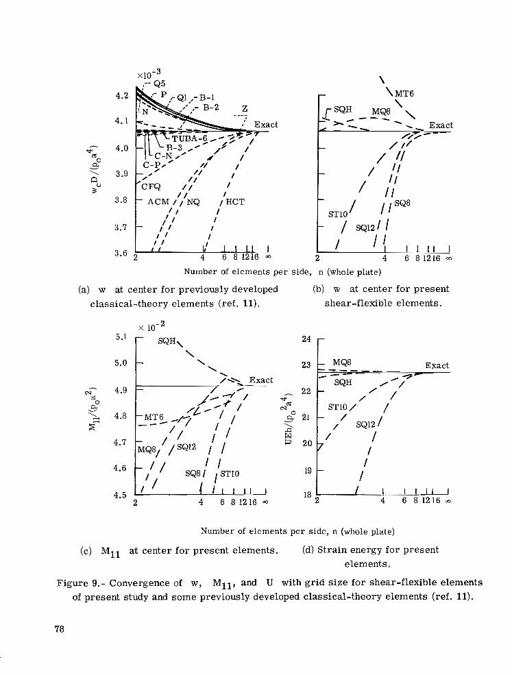
x ~ o - ~

4.2

4.1

h 4.0

‘ 3.9

B

cd a 0 v

4 3.8

3.7

3.6

\ \ MT6

Number of elements per side, n (whole plate)

(a) w at center for previously developed (b) w at center for present

classical-theory elements (ref. 11). s h e a r -flexible elements.

h

w cd

a 0

5 z-

5.1

5.0

4.9

4.8

4.7

4.6

\ -

-MT6 --- - /

23

h 22 9

@a cd

v a0 21 ... s 20

19 t I I 1 --u h 4 6 8 1216 m

/ ’ i l I I J I 4.5 2 4 6 8 1216 00

Number of elements per side, n (whole plate)

(c) MI1 at center for present elements. (d) S t ra in energy for present elements.

F igure 9.- Convergence of w, M l l , and U with gr id size for shear-flexible e lements of present study and some previously developed classical- theory elements (ref. 11).

78

SQ8-4 - 1.1 r 1.0

.9

.8

.7

.6

.5

.4

.3

.2

.1 'CI

g o al

SQ12 r

/ ..Z""" ................. --- . ...'..7

/ ; i

./ /

/ /

_/r- .... - / /. / - /.

/. / /

/ + /

._.. - /

- / - ; - / /.'. /

- - I' /

-

- i ; ; I'

- /'

/ /

/ - - - / - - i / -

/ - / / / ; -

/ - -

/' - /. ; -

- ; - i ; i

/ ;

/' - - /' /'

- - /' /'

- - - / ' /' - /. - -

/.'; I I t I I I I I I I I I I 1 1 2 3 4 5

SQH r

5 1.1

1.0 1

.9

.8

.7

.6

.5

4 - .3

.2

.1

0

- - ----_ - ............

i ......................... __--

.... //------ - /.* L /.

i - - /'

/' /

- /

/' /' /' -

- /

- /

- /' / - / - -

- / - - /

/' - -

/. /'

- - - /. -

/' - -

/' ./. - - - /' , I I I I I I I I I I

1 2 3 4 5 1 2 3 4 5 1 2 3 4 5

(a) Transverse displacement w at center.

wE,h3 1

Figure 10.- Effect of h/a on convergence of bending-moment resultant Mll and t ransverse displacement w 4 obtained by different stiffness and mixed models. Clamped, nine-layered, orthotropic square plate. CD

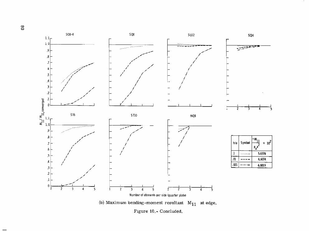
L 0

0.

S T6 + z- 1 1

.4

.3

.2

.1

0

L 0

0.

S T6 + z-

,,_..._.... .... ,. , . . ...‘

/- - / /

- /’

- /. /.

/ ‘ -

/

//’ I I

SQ12

r

l-

1-

STlO

- - -

I I I 1 1 2 3 4 5


(b) Maximum bending-moment resultant M11 at edge.

F igure 10.- Concluded.

l-

hla Symbol 7 x 10

.1 .. .. . .. ... 5.6376

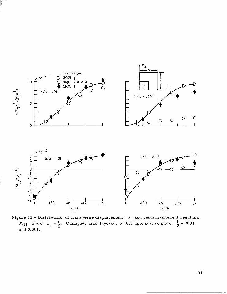
* cd a \

s!

w B

0 v

C-Y

F l:/

0 -

- converged 10-4 D SQH

h/a = .01

q a xl/a

Figure 11. - Distribution of t r a n s v e r s e displacement w and bending-moment resul tant Clamped, nine-layered, orthotropic squa re plate. $ = 0.01 M11 along x2 = a

2' and 0.001.

81

h -+ cd 0 a u \ 42 b w 3

c3

fiber orientation ( e / - e / e / - e / e / - e / e / - e / e /)

2 l-

14

12

10

8

6

4

-2 x 10 r

1 - 2 -

I I I I I I I I 1 I I I I I I I I 1 0 5 10 15 20 25 30 35 40 45 0 5 10 15 20 25 30 35 40 45

e , degrees (a) T r a n s v e r s e displacement w at center of plate. (b) Bending-moment resultant M11 at

center of plate.

F igure 12. - Effect of fiber orientation on response of simply supported, nine-layered, square anisotropic plate subjected to uniform normal p re s su re loading.

03 W

5'00

.05

5 10 15 20 25 30 35 40 45 0

.15 9.0

h

.13 8.0 cd

a

k

cu 0

5 w' 3 .ll 7.0

.09 6.0

.39 - h/a = 0.1

.37 - h/a = 0.01

3 / \ '35 0 5 10 15 20 25 30 35 40 45 G

3* .0070

h/a = 0.1

.0065

.0060 5 10 15 20 25 30 35 40 45

0, degrees

r h/a = 0.01 - 5 10 15 20 25 30 35 40 45

(c) Strain energy and measures of shear deformation and degree of anisotropy in plate as a function of fiber orientation.


:: [ .1

SQ12

/ i i i

/

- 3 1 .2 , I /*

.1

O 1 2 3 4 5

STlO

SQH

r

I 3 I h/a I Symbol I [wETh3/(poaI x 10 1 I I I

-1 ............. 3.7323 I I .01 I - - - - I 2.4079 I I .001 I ----- I 2.3943 I

t I 1 1 I

1 2 3 4 5

Number of elements pe r side (whole plate)

(a) T r a n s v e r s e displacement w at center .

F igure 13.- Effect of h/a on convergence of bending-moment resultant M11, t r a n s v e r s e displacement w, and s t ra in energy U obtained by higher o r d e r st iffness and mixed models. squa re plat e (4 5/- 45 /45 /- 4 5 /45 /-4 5 /4 5 /- 4 5/4 5).

Simply supported, nine-layered, anisotropic

84

MQ8 1.50 1- \ \

-

I I I I

I- SQ12 SQH

2 3 4 5 1 2 3 4 5 0 1

Number of elements per side (whole plate)

(b) Bending-moment resultant M11 at center.

Figure 13.- Continued.

MQ8 r

F

1.0

.9

.8

.7

.6

.5

.4

.3

.2

.1

0

h/a Symbol UETh/po 2 4 a

t-

c , 1 2 3 4 5

SQ12 r

e /

c i

.C /‘

i /’

/ *

/ * I

i 1 2 3 4 5

Number of elements per side (whole plate)

(c) Strain energy U in plate.


SQH r I-

I k I I

8.2997 X 1 f I e l I ........... I -- 1 I - - --Ii 5.1141 1

5.0809 X 10 -.-.- -

’ 1 2 3 4 5

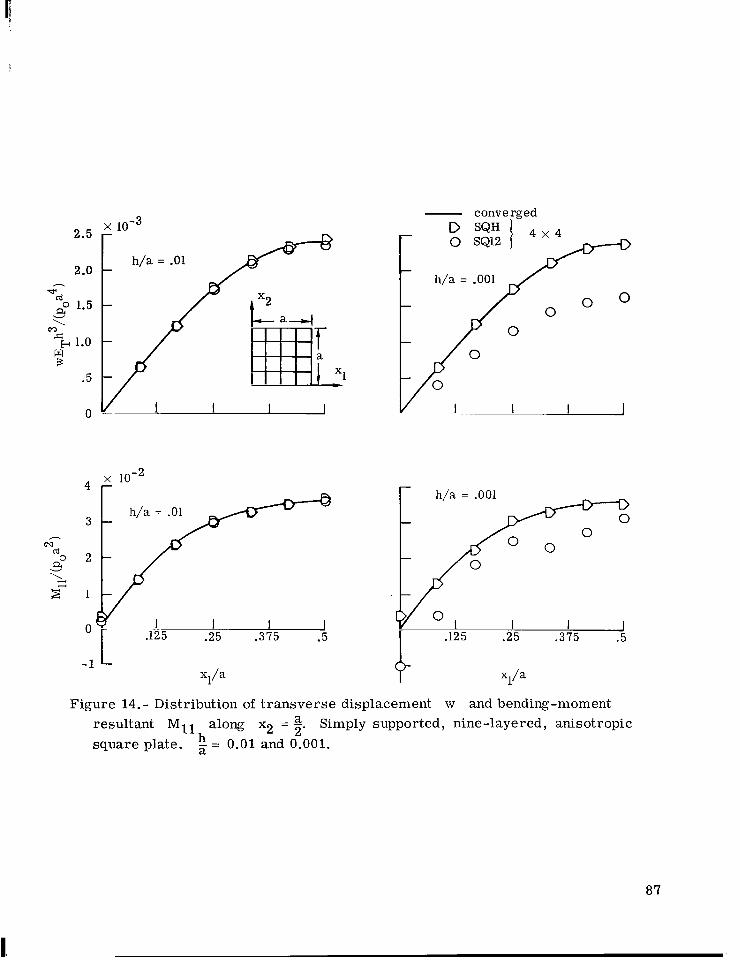
2.5

2.0

x 10-3 _.

h/a = .01

w cd

1.5

c F 1.0 w B

.5

7 m

V I I I 0 - I

x 4 r

h

c\1 cd a 0

T 2-

- converged

L- h/a = .001

I /- 0

. cp I I I

.25 .375 . 5 v O 1

I .125

Q Figure 14.- Distribution of t r a n s v e r s e displacement w and bending-moment

resultant Ml l along x2 = a Simply supported, nine-layered, anisotropic squa re plate.

2' = 0.01 and 0.001.

87

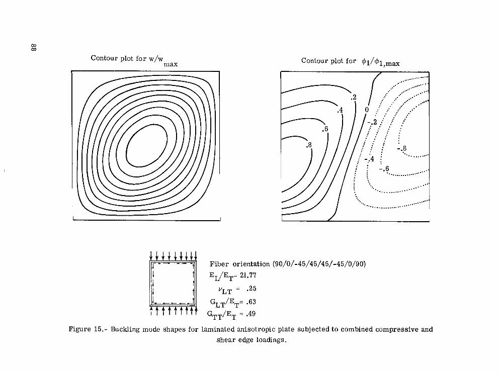
03 03

1 I 1 t 1 t

Contour plot fo r +l/$l,max

EL/ET= 21.77

vLT .25

F ibe r orientation (90/0/-45/4 5/4 5/-45/0/90)

GLT/ET= .63

' GTT/ET = .49

Figure 15.- Buckling mode shapes for laminated anisotropic plate subjected to combined compressive and shea r edge loadings.

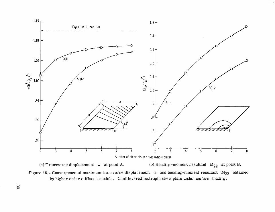
1.15

1.10

1.05

0 ==fm

= ̂ 1.00 m .c W 3

.95

.90

I

.85

Exper imen t ( re f . 38)

I 1 1 1 I J 3 4 5 6 7 8

1.5 -

1.4 -

1.3 -

1.2 -

N- 1.1 - 0

N

m a - .....

sN 1.0-

I I I I I 1 2 3 4 5 6 7 8

N u m b e r of e lements per side (whole plate)

(a) Transverse displacement w at point A. (b) Bending-moment resultant M22 at point B.

Figure 16. - Convergence of maximum transverse displacement w and bending-moment resultant M22 obtained by higher order st iffness models. Cantilevered isotropic skew plate under uniform loading.

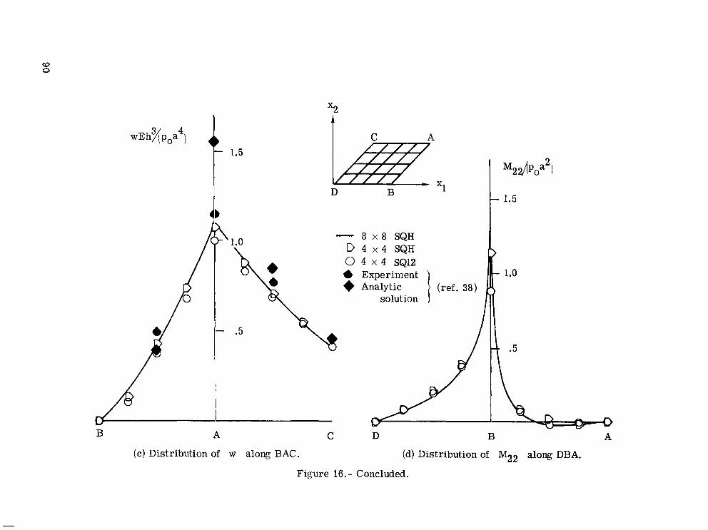
x2

D k$i53 B x1

8 x 8 SQH D 4 x 4 SQH 0 4 X 4 SQ12 6 Experiment

Analytic solution

-

(ref. 38)

b

- 1.0

I

A C D B A B

( c ) Distribution of w along BAC. (d) Distribution of M22 along DBA.


1 X

R/a = 10 f/a = 0.0125

E ~ / E ~ = 40 GLT/ET = 0.60

GTT/ET = 0.50

vLT = 0.25

Figure 17.- Charac te r i s t i c s of laminated graphite-epoxy shallow she l l s used in present study.

9 1

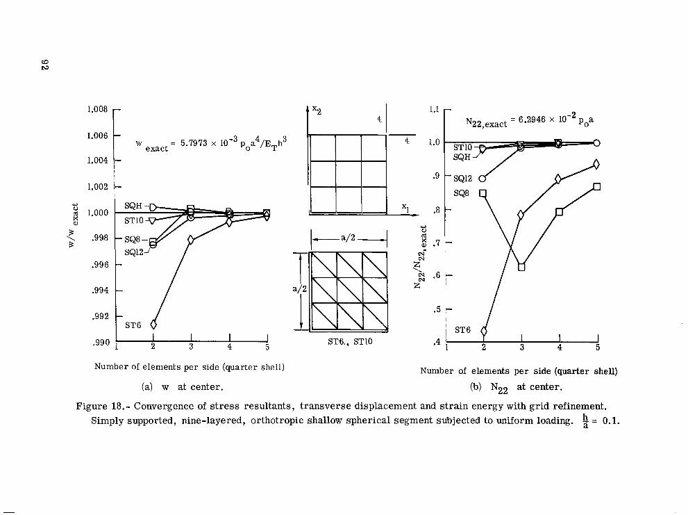
1.008

1.006

1.004

1.002

U ; 1.000 a,

3 \ .998 3

.996

.994

.992

.990

= 5.7973 x poa4/ETh 3 r w exact

t ,T6 d , I I I 1 1 2 3 4 5

Number of elements per side (quarter shell)

(a) w at center.

1"

ST6,, STlO

1.1

1.0

.9

.8

.7

.6

.5

.4

= 6.2946 x 10- 2 p,a N22, exact

1 c

1 c

1

' ST6

1 2 3 4 5 1 1 1


(b) NZ2 at center.

Figure 18. - Convergence of stress resultants, t r ansve r se displacement and s t ra in energy with grid refinement. Simply supported, nine-layered, orthotropic shallow spher ica l segment subjected to uniform loading. = 0.1.

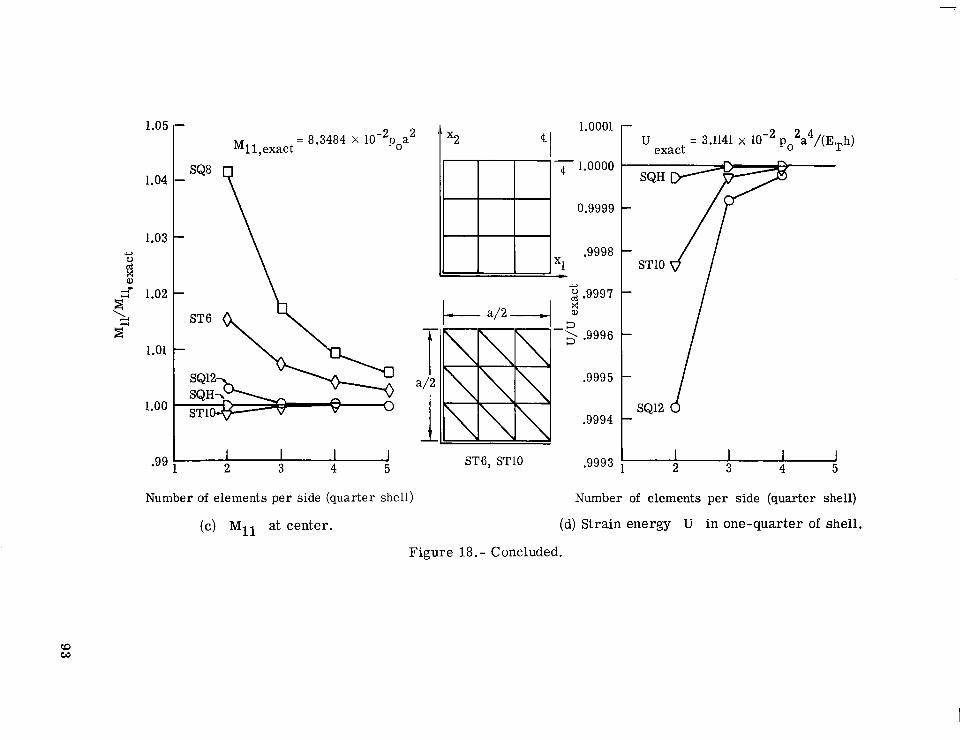
1.05 1.0001 - MI 1 ,exact poa t x 2 = 8.3484 x 10-

- g 1.0000

0.9999

.9998 x1 &

.99 , 2 3 4 5

I I -5 > .9996

.9995

2 2 4 U = 3.1141 x 10- p, a /(ETh) exact

t .9994 SQ12 d

5 ST6, STlO .9993 1 2 3 4 5

Number of elements per side (quarter shel l ) Number of elements per side (quarter shell)

(c) Mll at center. (d) Strain energy U i n one-quarter of shell.


1.10

1.05

1.00

.95

.90 c U

x m

SQ12

... . . . . . . . . . . . ___- - - - .._..... ..' /Y -...

0° \.-.-. /

I 1

S T6

.90 *95L 1

I I

/- /

/ /

/ V I 1 1 2 3 4 5

I I 1 I

S T l O


(a) T r a n s v e r s e displacement w a t center.

/=

I I I I 2 3 4 5

Figure 19. - Effect of h/a on convergence of t r a n s v e r s e displacement, s t r e s s resul tants , and s t r a i n energy obtained by different st iffness models. Simply supported, nine - laye r ed, orthot ropic shallow - spher ica l segment .

94

SQ12 1.2

1.0

.a

.6

.4

.2

c z o o? N N z -... N

zN 1.2

1.0

.8

.6

.4

.2

0

I I

I I 1 I I I

S T6

I 1 I I 2 3 4 5

I I I J

sno

- 2 3 4 5


(b) Membrane s t r e s s resul tant NZ2 at center .

F igu re 19.- Continued.

95

1.2

1.0

.8

.6

.4

.2

$ 0 m.

.-I-

.-I

I - 4

f 1.2

1.0

.8

.6

.4

.2

0

\. -

\ ...... ................................

\. /'

\ ,.'

./ a i -

/ /.

!

- \ .'.

-

-

-

I I 1 I

S T6

SQ12

I

I I

I I

I I 1 - I

sno

.... __---------

/' i

I I 1 I 2 3 4 5

SQH

i\. --- -j- - -- 1

i \. \.

i i i i i i i i i

I 1 1 I 2 3 4 s

hla I Symbol I 3 1 .1 8.3484~ lo-'

5.2390 x lo-' .01 ----

..........

I 7.3027x low4 I .001

Number of elements per side (quarter shel l )

(c) Bending-moment resul tant M11 at center .

F igure 19.- Continued.

96

1.02

1.00

L) .98 0 cd 2

3 \ 3

.96

.94

STlO

I 1 I

SQ12 -

I i i

I I

I

I I

.9 2 1


(d) Strain energy U in one-quarter of shell.


I I I I 1 2 3 4 5

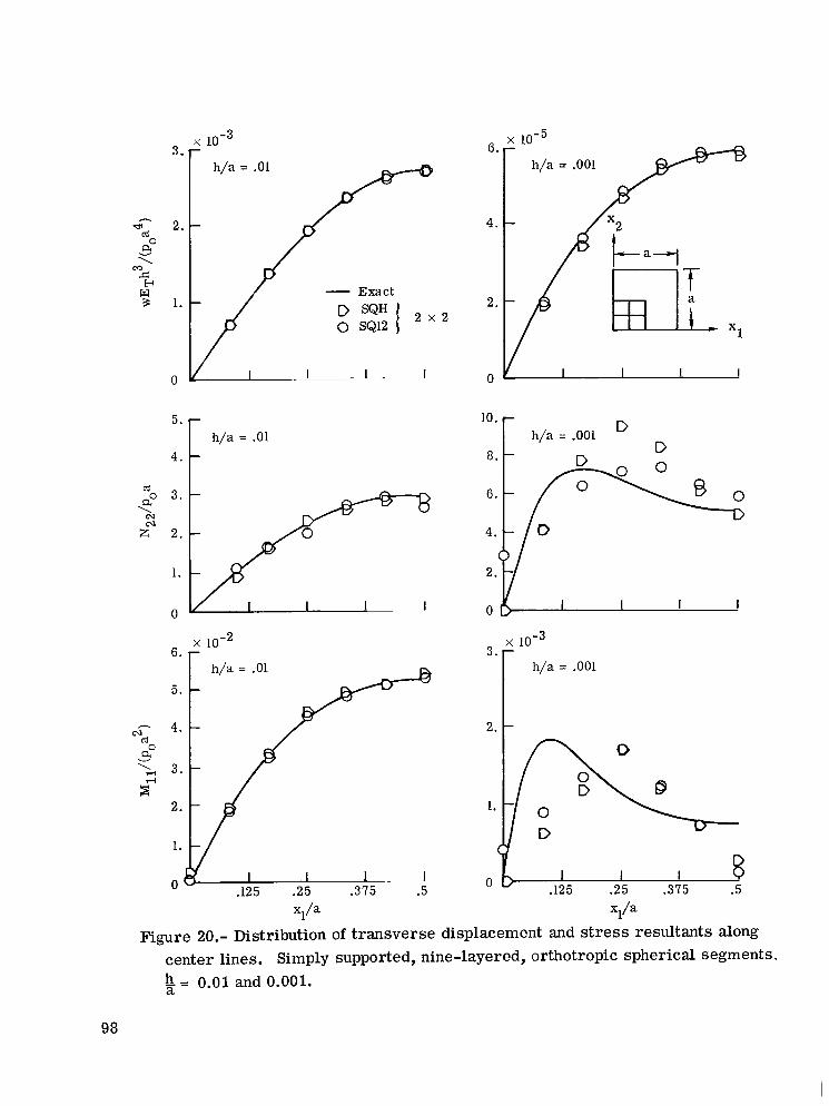
3.

h

w 2. cd a" 7

cc) s H w B 1.

0

. h/a = .01

- Exact

-P I I - - 1 , I

/

4 . 5* F h/a = aol

x 10-2 6. r

h

m d a 0 v

'+

6.

4.

2.

0 I I 1 I

h/a = .001

2.

I I I .125 .25 .375 .5 0

Figure 20.- Distribution of t r a n s v e r s e displacement and s t r e s s resul tants along center l ines , Simply supported, nine-layered, orthotropic spher ica l segments . h_ = 0.01 and 0.001. a

98

x 7 I-

- G '

4 %

I \ c E w

B

m

0 5 10 15 20 25 30 35 40 45 0 , degrees

(a) Transverse displacement w at center of shell.

Figure 21.- Effect of fiber orientation on response of a simply supported nine-layered, anisotropic spherical segment with a square planform subjected to uniform loading.

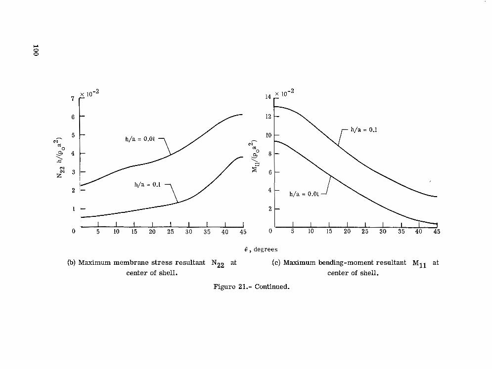
CJ h l- /

1 t 1 I I I 1 I

0 5 10 15 20 25 30 35 I I 1 I I I I

0 5 10 15 20 25 30 35 40 45 u

40 45

8 , degrees

(b) Maximum membrane stress resultant N22 at center of shell.

IC) Maximum bending-moment resultant Mll at center of shell.

Figure 21.- Continued.

.04 c .17 10 , .16 9

.15

.14

vn .13 cd

S I 0 $ .12

@ g .I1

.IO

.09

.08

0 5 10 15 20 25 30 35 40 45 0

r s3* r

h/a = OS1 7 .36

\

5 10 15 20 25 30 35 40 45

9, degrees

I-

- '00250 5 10 15 20 25 30 35 4 0 4 5

(d) Strain energy and measures of shear deformation and degree of anisotropy in shell as a function of fiber orientation.


CL 0 CL

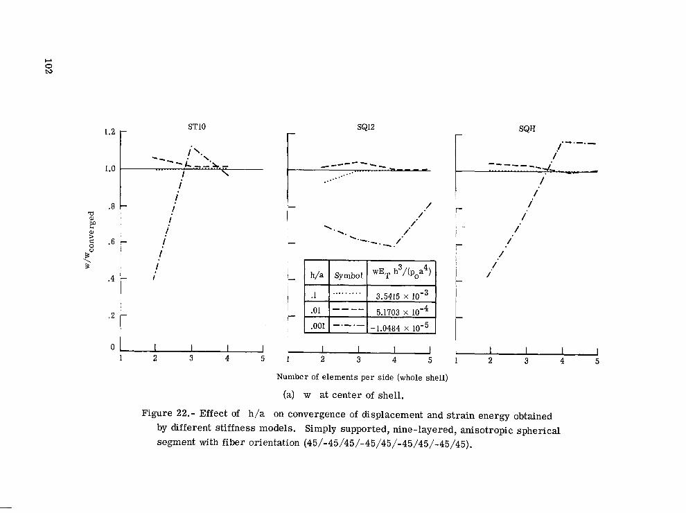
1.2

1.0

.8 a Q,

2

3*

5 .6

\ B

.4

.2

I I I I 1 2 3 4 5

Figure 22.- Effect of h/a

I I I I

I I I I I 1 2 3 4 5

1~ 1 2 3 4 5

Number of elements per side (whole shell)

(a) w a t center of shell.

on convergence of displacement and s t ra in energy obtained by different st iffness models. Simply supported, nine-layered, anisotropic spherical segment with f iber orientation (45/-45/45/-45/45/-45/45/-45/45).

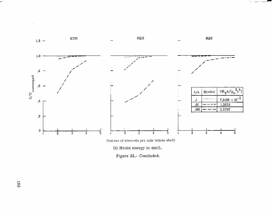
1.2 :- I

STlO

4-- 1.0

.2 t * 1 2 3 4 5

0

SQ12 I-

SQH

1 2 3 4 5 1 2 3 4 5

Number of elements per side (whole shell)

(b) Strain energy in shell.


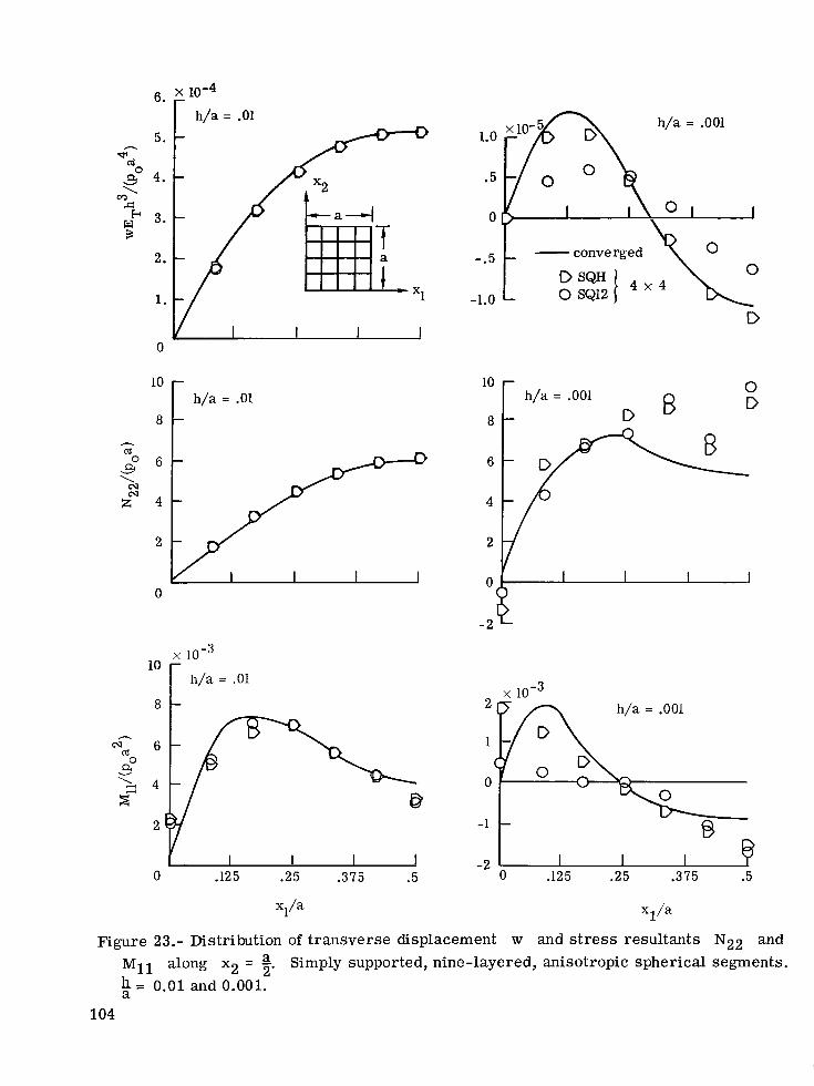
6. x 10-4 r h/a = .01

c dl cd

\ .so m .c k

w' 3

h

cd

a 0

x zm

5. t- '

4 * t Ax2 I RT; I I I

0

0

8

I I I I 0 .125 .25 .375 .5

1.0

.5

0

-.5

-1.0

1 I \ \

D

10 I- n

8 h/a = .001 8 D

v D

f? -1 nfi 4v 2

" I w/

-

-1 -

0 .125 .25 .375 .5

xl/a xl/a

Figure 23.- Distribution of t r a n s v e r s e displacement w and s t r e s s resul tants N22 and Simply supported, nine-layered, anisotropic spherical segments. M1 along x2 = a 2'

= 0.01 and 0.001.

104

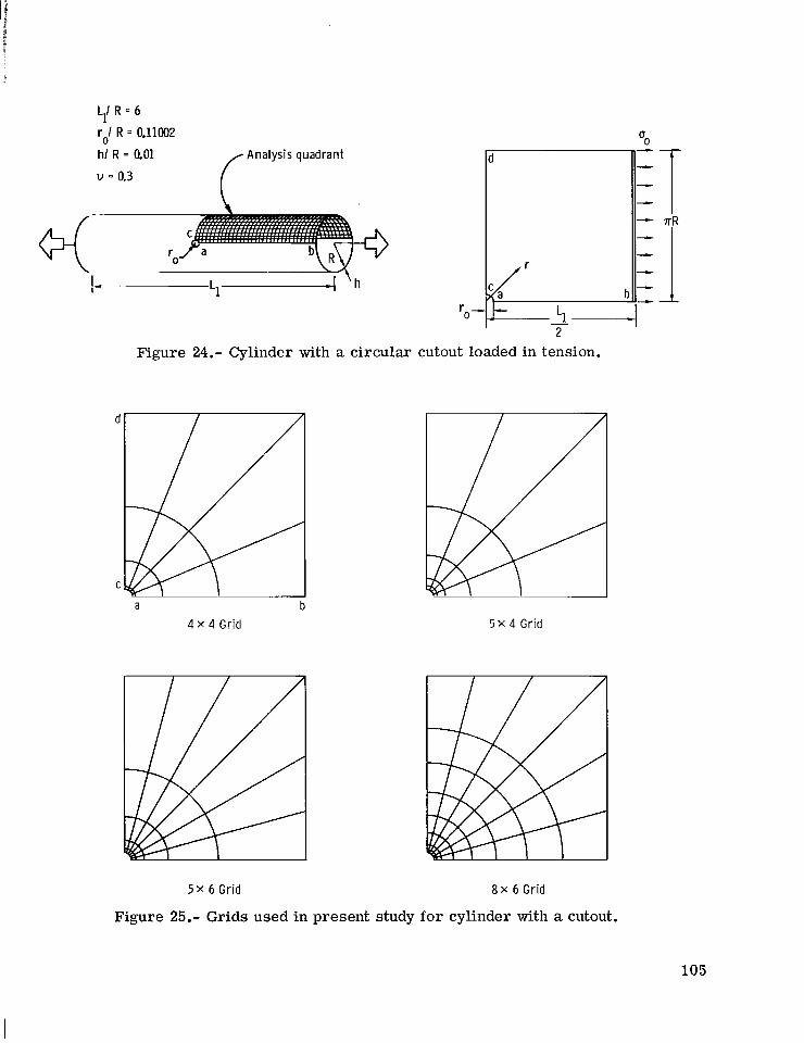
5 l R . 6 r d R = 0.11002 hl R = 0.01 v = 0.3

/Ana lys is quadrant

Figure 24.- Cylinder with a c i rcu lar cutout loaded in tension.

a b 4 x 4 Grid 5x 4 Grid

5x 6 Grid 8 x 6 Grid

Figure 25.- Gr ids used in p re sen t study for cylinder with a cutout.

105

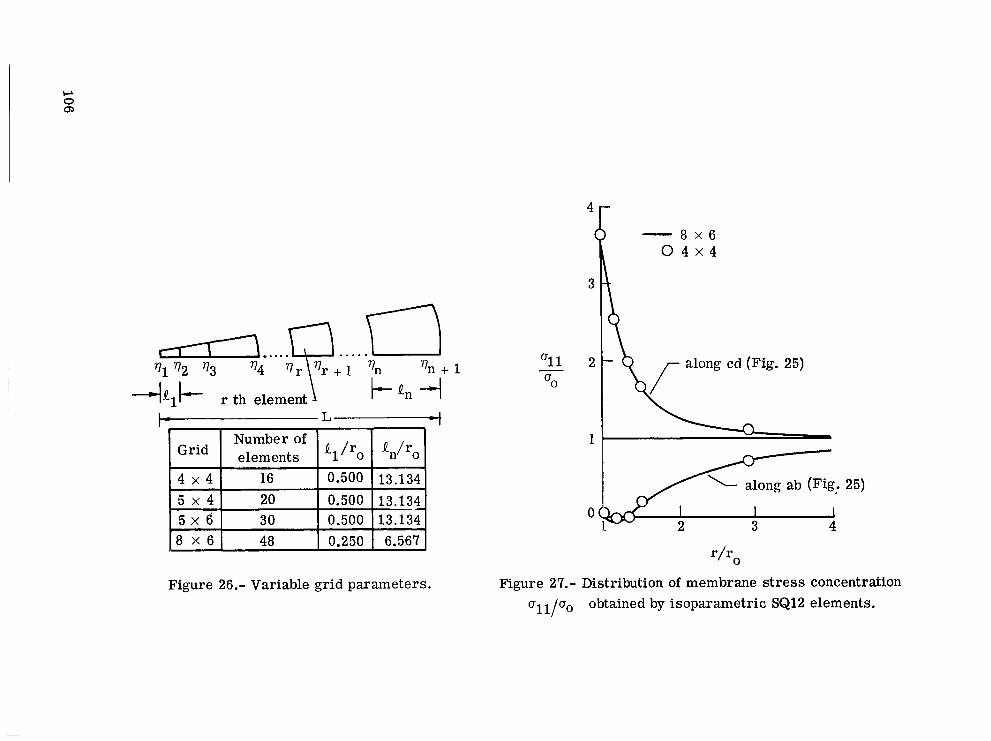
d .... \-I.. . . 771 772 773

d Q 1 b r th

77, 77, + b n -1

Grid Number of I elements

8 X 6

Figure 26.- Variable gr id parameters .

1

4l - 8 x 6

O 1 1

1 along ab (Fig. 25) I

0 I 1 I 2 3 4

Figure 27.- Distribution of membrane stress concentration

ul1/u0 obtained by i soparamet r ic SQ12 elements.

h/R = .05

Ll/R = 2

f' 1..

7rR/4

,Figure 28.- Charac te r i s t ics of two-layered graphite-epoxy cylinders.

@

-

@ -L 1/2 -

\Analysis octant

'm \ I \

\ I I I

n = 2 @

-L /2+ 1 4L

Grid 1

n = 4

Gr id 2

F igure 29.- Gr ids and modes for orthotropic cylinder.

107

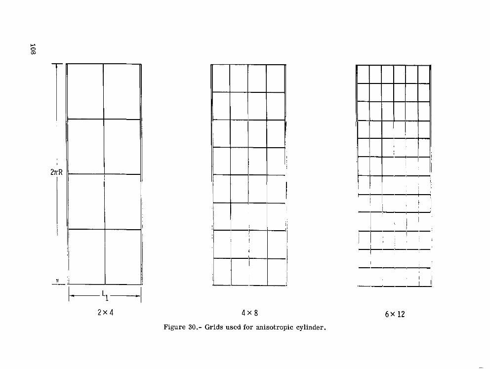
4x8

Figure 30.- Grids used for anisotropic cylinder.

6x 12

W

6 x 12

2 U

0.5816

Grid

I 4 x 8 I 0.6028 I

Figure 31.- Fundamental mode shapes and frequencies for simply supported, two-layered, anisotropic graphite - epoxy cylinder.

w 0 (D

WASHINGTON. - D.C. 20546 POSTAGE A N D FEES P A I D [S) NATIONAL AERONAUTICS AND SPACE ADMINISTRATION

N A T I O N A L AERONAUTICS A N D OFFICIAL BUSINESS SPACE A D M I N I S T R A T I O N

PENALTY FOR PRIVATE USE $300 SPECIAL FOURTH-CLASS RATE 451 U S M A I L

BOOK

169 0 0 1 C 1 U D ?+5C107 S00503DS DEPT O F THE AI9 F O R C E AF WEAPONS 1. A M G H A T O R Y A’T‘ Ih’ : T E C H N I C A L L I E R A H Y ( S U L ) K T P T L A N D 3 F U t4Pl 87117

. I . , , ? ’ POSTMASTER . - I ‘ I : If Un~elive‘rnble (Section 158 . - Postal hlariiiiil) Do Not Return :r-> ’ _ . . . . .,

, _ . . ’ :,, .

.*- * > ; :, --_ .I I

‘“The aeronautical and space activities of the United States shall be conducted so as to contribute . . . t o the expansion of hziman knowledge of phenomena in the atmosphere and space. T h e Administration shall provide for the widest practicable and appropriate dissemimtion of information concerning its pcjivities. and the results the;eo+f.”

- ~ A T I O N A L AERO~AUTICS AND S’PACI~’AACT OF 1958 .

NASA SCIENTIFIC AND TECHNICAL PUBLICATIONS TECHNICAL REPORTS: Scientific and technical information considered important, complete, and a lasting contribution to existing knowledge.

TECHNICAL NOTES: Information less broad in scope but nevertheless of importance as a contribution to existing knowledge.

TECHNICAL MEMORANDUMS : Information receiving limited distribution because of preliminary data, security classifica- tion, or other reasons. Also includes conference proceedings with either limited or unlimited distribution.

CONTRACTOR REPORTS: Scientific and technical information generated under a NASA contract or grant and considered an important contribution to existing knowledge.

-

TECHNICAL TRANSLATIONS: Information published in a foreign language considered to merit NASA distribution in English.

SPECIAL PUBLICATIONS: Information derived from or of value to NASA activities. Publications include final reports of major projects, monographs, data compilations, handbooks, sourcebooks, and special bibliographies.

TECHNOLOGY UTILIZATION PUBLICATIONS: Information on technology used by NASA that may be of particular interest in commercial and other- non-aerospace applications. Publications include Tech Briefs, Technology Utilization Reports and Technology Surveys.

Details on the availabilify of these publications may be obtained from:

SCIENTIFIC AND TECHNICAL INFORMATION OFFICE

N A T I O N A L A E R O N A U T I C S A N D SPACE A D M I N I S T R A T I O N Washington, D.C. 20546

Shear-flexible finite-element models of laminated ... · nasa technical note d a 0 7 n z c -loan...

Documents

Transcript of Shear-flexible finite-element models of laminated ... · nasa technical note d a 0 7 n z c -loan...