Shear centre eccentricity in SCIA EngineerDelft University of Technology

Gert Wilgenburg

June 2021

Preface

This thesis is the final project for the Bachelor Civil Engineering at the Delft Univer-sity of Technology, where I investigated an error in the framework analysis softwareSICA engineer regarding shear centre eccentricity.

I want to thank dr. ir. P.C.J. Hoogenboom for his support throughout this project.His experience and knowledge were extremely helpful. I also want to thank dr. M.Veljkovic for helping with the assessment. Finally, I want to thank Simon Top forturning my sketches into wonderful illustrations.

Delft, June 13, 2021Gert Wilgenburg

i

Summary

Torsional moments and shear stresses are not calculated correctly in the frameworkanalysis software SCIA Engineer for cross-sections with a shear centre eccentricity.The aim of this research is to analyze and solve this problem. This thesis is com-posed of five chapters. Chapter 1 is introductory and describes the solution strategyand observations done by others. Chapter 2 compares hand calculations with SCIAand also with the engineering software Ansys. All calculations are executed using acantilever beam with a channel section. Chapter 3 dives deeper into the calculationapproach in SCIA to get a better understanding of where the error arises withinthe program. Chapter 4 is an analysis of the safety risks. Conclusions are drawn inChapter 5.

It was established that Ansys calculates the correct results for the cantilever beamwith a shear centre eccentricity, whereas SCIA does not. SCIA has an option called’consider torsion due to shear centre eccentricity’ which was found to be workingcorrectly, also for statically indeterminate beams. However, the option can be con-fusing and is hidden within the calculation results. Also, it can only report shearstresses and no torsional moments or rotations. The author suggests that SCIAshould move the system line to the normal force centre. The self weight has to beapplied in the normal force centre as well.

ii

Contents

Preface i

Summary ii

1 Introduction 11.1 The problem . . . . . . . . . . . . . . . . . . . . . . . . . . . . . . . . . . 11.2 Solution strategy . . . . . . . . . . . . . . . . . . . . . . . . . . . . . . . . 11.3 Work by others . . . . . . . . . . . . . . . . . . . . . . . . . . . . . . . . . 2

2 Comparison 42.1 Cross-sectional properties . . . . . . . . . . . . . . . . . . . . . . . . . . . 42.2 Hand calculation . . . . . . . . . . . . . . . . . . . . . . . . . . . . . . . . 52.3 Results in SCIA . . . . . . . . . . . . . . . . . . . . . . . . . . . . . . . . 62.4 Results in Ansys . . . . . . . . . . . . . . . . . . . . . . . . . . . . . . . . 82.5 Conclusion . . . . . . . . . . . . . . . . . . . . . . . . . . . . . . . . . . . . 9

3 Stiffness Method 103.1 Stiffness matrix . . . . . . . . . . . . . . . . . . . . . . . . . . . . . . . . . 103.2 Results . . . . . . . . . . . . . . . . . . . . . . . . . . . . . . . . . . . . . . 113.3 Conclusion . . . . . . . . . . . . . . . . . . . . . . . . . . . . . . . . . . . . 15

4 Safety 164.1 Dangers . . . . . . . . . . . . . . . . . . . . . . . . . . . . . . . . . . . . . 164.2 Practical examples . . . . . . . . . . . . . . . . . . . . . . . . . . . . . . . 174.3 Conclusion . . . . . . . . . . . . . . . . . . . . . . . . . . . . . . . . . . . . 18

5 Conclusion and recommendations 195.1 Calculation comparison . . . . . . . . . . . . . . . . . . . . . . . . . . . . 195.2 Solution using the Stiffness Method . . . . . . . . . . . . . . . . . . . . . 195.3 Recommendations . . . . . . . . . . . . . . . . . . . . . . . . . . . . . . . 20

Bibliography 21

Appendices 23

A Hand calculations 24A.1 Cross-sectional properties . . . . . . . . . . . . . . . . . . . . . . . . . . . 24A.2 Shear centre and shear stresses . . . . . . . . . . . . . . . . . . . . . . . 28

iii

B Stiffness Method 31B.1 Solution strategy . . . . . . . . . . . . . . . . . . . . . . . . . . . . . . . . 31B.2 Maple file - hand calculation properties . . . . . . . . . . . . . . . . . . 36B.3 Maple file - SCIA properties . . . . . . . . . . . . . . . . . . . . . . . . . 40

iv

Chapter 1

Introduction

Beams and columns in constructions can be subjected to torsional moments. It wasfound that these moments are not calculated correctly in the framework analysissoftware SCIA Engineer (Drillenburg, 2017). The software engineers were notified,but the error was not removed. In this project we will continue the research on thisproblem.

1.1 The problem

We want to investigate what exactly goes wrong with the calculations in SCIA.Therefore, we first need to look into the problem in more detail.

Gravity acts through the normal force centre of a cross-section1. In cross-sectionswith only one axis of symmetry the normal force centre does not coincide with theshear centre. Forces which do not act through the shear centre will result in torsion.A cantilever with a channel section will therefore rotate around its axis (Welleman,2021). In SCIA however, this does not happen.

To investigate where the error arises within the program, Drillenburg consideredthree parameters to check for possible discrepancies: geometry of cross-sections,different boundary conditions and different load cases. It was established that theproblems with torsion only occur if there is an eccentricity of the shear centre.

1.2 Solution strategy

We will consider a channel section acting as a cantilever beam for every calculationthroughout this research. The dimensions are given in Figure 1.1 and are based onan UPE 220 steel profile, the length of the beam is 5 meters. The material proper-ties are listed in Table 1.1. In the next chapter we will compare hand calculationswith SCIA and another software package Ansys. Chapter 3 will revolve around thecomputational method SCIA uses and offers possible solutions for the error. Finallywe will investigate if this error could potentially lead to dangerous situations.

1Note that the normal force centre differs from the centre of gravity for an inhomogeneous cross-section. It is defined as the location where the normal force only causes strains and no curvatures.

1

y

z

xy

tw= 8

tf= 12

220

85

53.1825.77

z

NCSC

A

B

dimensionsin mm

Figure 1.1: Dimensions of a channel section

Table 1.1: Material properties

Parameter Symbol Value UnitDensity ρ 7850 kg/m3

Young’s Modulus E 210 GPaShear Modulus G 80769 MPaYield Strength σy 235 MPa

Ultimate Tensile Strength σult 360 MPa

1.3 Work by others

Drillenburg used an L-shaped cross-section for his research. He looked at SCIA’sresponse to different geometries, boundary conditions and load cases. His findingsare summarized and later on used for comparison.

2

SCIA’s behavior according to Drillenburg is summarized below. In the next chapterwe will check if these observations are valid or not.

Geometry

• Cross-sections which are symmetrical in two axes show no discrepancies com-pared with the expected values.

• Cross-sections which are symmetrical in one axis show no significant discrep-ancies compared with the expected values, only the position of the shear centrediffers slightly.

Boundary Conditions

• A single clamped cantilever beam loaded in pure torsion shows no discrepanciescompared with the expected values.

• A double clamped beam loaded in pure torsion shows no discrepancies com-pared with the expected values. This is also true if the torsional moment isapplied at different positions along the beam.

Loading

• A beam loaded in pure bending shows no discrepancies compared with theexpected values.

• A beam loaded with a point load in the normal force centre shows no torsionaldeformation and no internal moment around the x-axis. The shear stress inthis situation did not match the expected value.

• A beam loaded with a point load in the shear centre shows torsional deforma-tion, whereas pure bending is expected.

Additional

• Using the option ‘consider torsion due to shear centre eccentricity’ does notgive the correct magnitude for the torsional shear stress.

3

Chapter 2

Comparison

In this chapter we will compare hand calculations with SICA’s output and calcula-tions made with the engineering simulation software Ansys. Two situations will beconsidered: one where the self weight acts through the normal force centre and onewhere an equivalent line load acts through the shear centre of the channel section.All hand calculations are made using Maple and can be found in Appendix A.

2.1 Cross-sectional properties

From Appendix A.1 we obtain the cross-sectional properties. These properties arealso reported in Table 2.1. The cross-sectional properties that are obtained usingSCIA and Ansys are listed in this table as well. The location of the normal forcecentre is given with respect to point A in Figure 1.1 using a coordinate system asindicated in the same figure. The location of the shear centre is given with respectto the normal force centre and is obtained using Appendix A.2.

Table 2.1: Cross-sectional properties

Hand calculation SCIA AnsysNC (25.77 mm; -110 mm) (25.77 mm; 110 mm) (25.77 mm; 110 mm)A 3608 mm2 3608 mm2 3608 mm2

Iyy 2.55 ⋅ 106 mm4 2.55 ⋅ 106 mm4 2.55 ⋅ 106 mm4

Izz 2.71 ⋅ 107 mm4 2.71 ⋅ 107 mm4 2.71 ⋅ 107 mm4

Iyz 0 0 0It 1.24 ⋅ 105 mm4 1.25 ⋅ 105 mm4 1.26 ⋅ 105 mm4

SC (53.18 mm; 0) (52.89 mm; 0) (52.87 mm; 0)

The only noticeable differences in the table are the values for the torsional constantand the location of the shear centre. The torsional constant It for a channel sectioncan be calculated using approximation equations. Applying a simple thin-walledapproach would result in a value of 1.35 ⋅105 mm4 which is rather high compared tothe results of SCIA and Ansys. Using an extensive formula from the book Roark’sformulas for stress and strain gives a more pleasant result as can be seen in the table.The difference in the location of the shear centre is a result of a different calculationapproach. SCIA and Ansys calculate this location using the Finite Element method.For the hand calculation, a simple case of equilibrium is assumed (Appendix A.2).

4

2.2 Hand calculation

The hand calculation starts with the determination of the cross-sectional propertieswhich has been done in the previous section. Additional to the cross-sectional prop-erties from Table 2.1, the self weight of the beam is needed which can be calculatedusing Equation 2.1.

qz = A ⋅ ρ ⋅ g = 3608 ⋅ 7850 ⋅ 9.81 ⋅ 10−9 = 0.278 N/mm (2.1)

If the self weight would act through the shear centre, no torsional moment androtation can occur. The deflection of the beam can then be calculated using oneof the vergeet-mij-nietjes (’forget-me-nots’) for a single clamped beam, since it willonly deflect in the z-direction (Hartsuijker, 2016).

uz =qz ⋅ l4

8EIzz=

0.278 ⋅ 50004

8 ⋅ 5.69 ⋅ 1012= 3.81 mm (2.2)

In reality, the self weight of the beam acts through the centroid which coincides withthe normal force centre in this case. We know that for the channel section the normalforce centre and shear centre do not coincide, therefore a torsional moment will act onthe beam. The maximum torsional moment at the clamped edge can be calculatedby multiplying the self weight with the length of the beam and subsequently withthe shear centre eccentricity. The beam will now rotate around the x-axis due tothe presence of the torsional moment. The maximum rotation of a cantilever beamloaded with an uniform torque can be calculated using Equation 2.3 (James F.Lincoln Arc Welding Foundation, 2021).

ϕx =Mx ⋅ l

2 ⋅GIt=−7.39 ⋅ 104

⋅ 5000

2 ⋅ 80769 ⋅ 1.24 ⋅ 105= −18.45 mrad (2.3)

The beam will now also deflect in the y-direction because of the rotation. The totaldeflection in the y- and z-direction can be calculated by adding the contribution ofthe rotation to the earlier calculated deflections for pure bending. Small rotationsare assumed and axial deformation is neglected.

The results of the hand calculation are listed in Table 2.2. The displacements aregiven with respect to point B in Figure 1.1. The reader is encouraged to consultAppendix A for more detailed calculations.

Table 2.2: Hand calculation results

Loading in NC Loading in SCuy -2.03 mm 0uz 4.32 mm 3.81 mmϕx -18.45 mrad 0Mx −7.39 ⋅ 104 Nmm 0τtor 7.15 N/mm2 0

5

2.3 Results in SCIA

We construct the channel section in SCIA and change the local coordinate systemto the same coordinate system that has been used for the hand calculation. We thenadd the self weight as a line load to the beam so the position of this load can bechanged. We emulate the load in the shear centre by disabling the self weight of thestructure and moving the line load to the shear centre using an offset. SCIA cannow calculate and graphically display the displacements and stresses. For calculat-ing the shear stress, the option ’consider torsion due to shear centre eccentricity’ isleft unchecked for both load cases. The maximum value of the torsional shear stresswith this option enabled is given between parenthesis in Table 2.3.

Table 2.3: SCIA results

Loading in NC Loading in SCuy 0 2.01 mmuz 3.84 mm 4.33 mmϕx 0 18.20 mradMx 0 7.35 ⋅ 104 Nmmτtor 0 (−7.06 N/mm2

) 7.06 N/mm2(0)

We want to check Drillenburg’s statement that using the option ’consider torsion dueto shear centre eccentricity’ gives incorrect torsional shear stresses. By comparingTable 2.2 with Table 2.3 we can conclude that this is not the case for a cantileverbeam with a channel section. We will now add a fixed support at the other end ofthe beam to make it statically indeterminate and redo the calculation in SCIA.

Figure 2.1: Torsional shear stress due to the self weight with the option ’considertorsion due to shear centre eccentricity’ enabled

From Figure 2.1 we can observe that the maximum torsional shear stress at theflange equals 3.53 N/mm2 and at the centre of the web 2.35 N/mm2.

6

To obtain the torsional stress at the clamped edges using a hand calculation, we useEquation A.13 and A.14 from Appendix A.2 and take 1

2Mx for Mt.

τf ;max = ∣

12Mx ⋅ tf

It∣ = ∣

12 ⋅ −7.39 ⋅ 104

⋅ 12

1.24 ⋅ 105∣ = 3.58 N/mm2 (2.4)

τw;max = ∣

12Mx ⋅ tw

It∣ = ∣

12 ⋅ −7.39 ⋅ 104

⋅ 8

1.24 ⋅ 105∣ = 2.38 N/mm2 (2.5)

These values therefore match with SCIA’s output2. This strongly suggests thatDrillenburg’s statement is incorrect.

We can now conclude the following regarding SCIA’s calculations:

• SCIA reports no torsional moment and no rotation when the system is loadedin the normal force centre.

• SCIA reports a torsional moment and a rotation when the system is loaded inthe shear centre whereas pure bending is expected.

• The reported rotation is positive which indicates that the system rotates anti-clockwise, see Figure 2.2. This is due to the fact that the line load is nowphysically moved to the shear centre and is treated as an eccentric load.

• Using the option ’consider torsion due to shear centre eccentricity’ when load-ing the system in the normal force centre results in the same torsional shearstresses as can be found when moving a line load to the shear centre, butwith an opposite sign. Using this option when loading the system in the shearcentre results in zero stress. It was established that the option also workscorrectly for a statically indeterminate beam.

Figure 2.2: Axial rotation due to a line load in the shear centre in SCIA

2Note that the decimals are slightly different, because the torsional constant and shear centrecoordinates differ as well (Table 2.1).

7

One last point to mention about the option ’consider torsion due to shear centreeccentricity’ is that it is only applicable for finding stresses and strains and notdisplacements or rotations. In Chapter 3 we will try to solve this problem, but wewill first look at the results in Ansys.

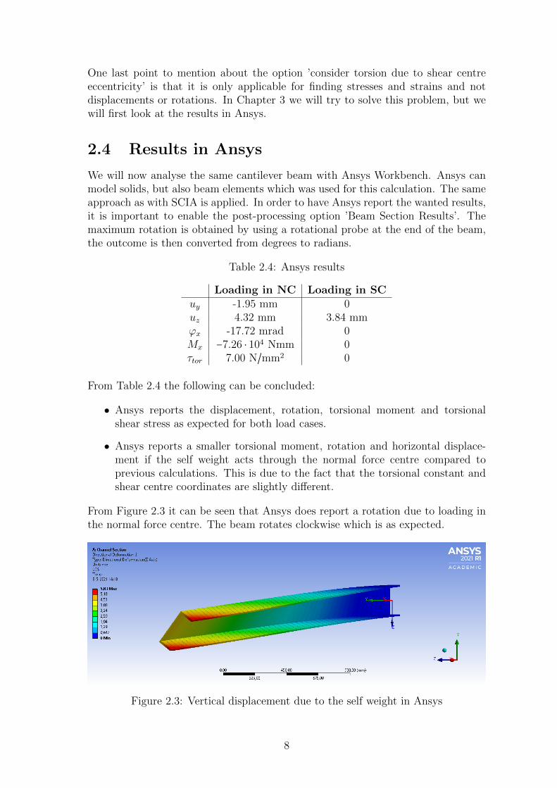
2.4 Results in Ansys

We will now analyse the same cantilever beam with Ansys Workbench. Ansys canmodel solids, but also beam elements which was used for this calculation. The sameapproach as with SCIA is applied. In order to have Ansys report the wanted results,it is important to enable the post-processing option ’Beam Section Results’. Themaximum rotation is obtained by using a rotational probe at the end of the beam,the outcome is then converted from degrees to radians.

Table 2.4: Ansys results

Loading in NC Loading in SCuy -1.95 mm 0uz 4.32 mm 3.84 mmϕx -17.72 mrad 0Mx −7.26 ⋅ 104 Nmm 0τtor 7.00 N/mm2 0

From Table 2.4 the following can be concluded:

• Ansys reports the displacement, rotation, torsional moment and torsionalshear stress as expected for both load cases.

• Ansys reports a smaller torsional moment, rotation and horizontal displace-ment if the self weight acts through the normal force centre compared toprevious calculations. This is due to the fact that the torsional constant andshear centre coordinates are slightly different.

From Figure 2.3 it can be seen that Ansys does report a rotation due to loading inthe normal force centre. The beam rotates clockwise which is as expected.

Figure 2.3: Vertical displacement due to the self weight in Ansys

8

2.5 Conclusion

We looked at the channel section cantilever from Figure 1.1 loaded due to its selfweight and compared the calculation results from a hand calculation, SCIA andAnsys. A summary of the results for the normal situation (i.e. self weight throughNC) is given in Table 2.5, a summary of the results for an equivalent line load inthe shear centre is given in Table 2.6. Again, the output with the option ’considertorsion due to shear centre eccentricity’ enabled is given between parentheses.

Table 2.5: Comparison - loading in NC

Hand calculation Ansys SCIAuy -2.03 mm -1.95 mm 0uz 4.32 mm 4.32 mm 3.84 mmϕx -18.45 mrad -17.72 mrad 0Mx −7.39 ⋅ 104 Nmm −7.26 ⋅ 104 Nmm 0τtor 7.15 N/mm2 7.00 N/mm2 0 (−7.06 N/mm2

)

Table 2.6: Comparison - loading in SC

Hand calculation Ansys SCIAuy 0 0 2.01 mmuz 3.81 mm 3.84 mm 4.33 mmϕx 0 0 18.20 mradMx 0 0 7.35 ⋅ 104 Nmmτtor 0 0 7.06 N/mm2

(0)

The results of Ansys are somewhat different compared to the hand calculation, butthis is mainly due to the use of a slightly different torsional constant. The programdoes show the correct behavior for the system with the axial rotation being clock-wise. SCIA however, shows remarkable behavior and this has to be investigatedfurther.

We can observe the following:

• It is possible that SCIA makes the assumption that shear forces always actthrough the shear centre. This could explain the discrepancies for the con-sidered channel section, because its shear centre does not coincide with thenormal force centre.

• Drillenburg concluded that using the option ’consider torsion due to shear cen-tre eccentricity’ reports incorrect magnitudes for the torsional shear stresses.This statement is not true for a channel section, as the magnitude for thetorsional shear stress matches with the expectation. The option also workscorrectly for a statically indeterminate beam.

We will use these observations in the next chapter to search for the origin of theproblem and the possible solutions.

9

Chapter 3

Stiffness Method

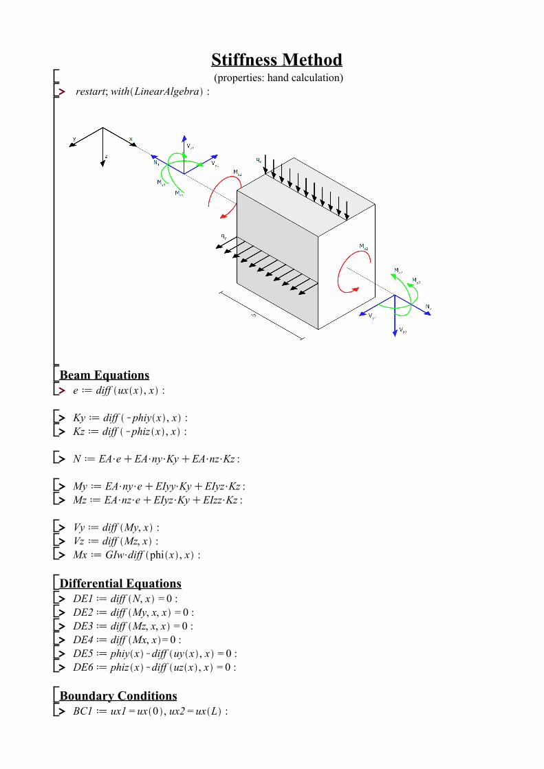
SCIA incorporates Finite Element technology to create a global stiffness matrix Kfrom elemental stiffness matrices. The coefficients in a stiffness matrix link the forcesand moments to the displacements and rotations. In this chapter we will constructthe stiffness matrix for a three dimensional beam element and use it to compute theunknown displacements and rotations for the cantilever with the channel section.We call this solution procedure the Stiffness Method.

3.1 Stiffness matrix

For the establishment of the stiffness matrix, the Euler-Bernoulli beam theory isconsidered and expanded with the theory of Saint-Venant for torsion. This meansthat linear elastic behavior is expected and shear deformation and restrained warp-ing are neglected. In SCIA we made the same assumptions when comparing theoutput to the hand calculation and Ansys.

We will use the following eight steps to construct and solve the stiffness matrix:

1. Define a coordinate system for internal and external forces for a 3D beamelement.

2. Define the equations for the beam properties.

3. Set up the differential equations and boundary conditions.

4. Solve the system.

5. Substitute the solution back into the previously defined equations.

6. Set up the forces and moments on both ends of the beam element.

7. Determine the stiffness matrix coefficients by differentiating the loading atboth ends of the beam element to the unknown displacements and rotations.

8. Solve the system for the unknown displacements and rotations by applyingknown forces, moments, displacements and rotations.

A detailed elaboration on this solution strategy is given in Appendix B.1. Thecorresponding Maple calculation file can be found in Appendix B.2.

10

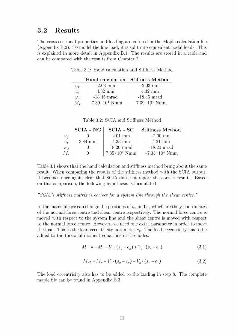
3.2 Results

The cross-sectional properties and loading are entered in the Maple calculation file(Appendix B.2). To model the line load, it is split into equivalent nodal loads. Thisis explained in more detail in Appendix B.1. The results are stored in a table andcan be compared with the results from Chapter 2.

Table 3.1: Hand calculation and Stiffness Method

Hand calculation Stiffness Methoduy -2.03 mm -2.03 mmuz 4.32 mm 4.32 mmϕx -18.45 mrad -18.45 mradMx −7.39 ⋅ 104 Nmm −7.39 ⋅ 104 Nmm

Table 3.2: SCIA and Stiffness Method

SCIA - NC SCIA - SC Stiffness Methoduy 0 2.01 mm -2.00 mmuz 3.84 mm 4.33 mm 4.31 mmϕx 0 18.20 mrad -18.20 mradMx 0 7.35 ⋅ 104 Nmm −7.35 ⋅ 104 Nmm

Table 3.1 shows that the hand calculation and stiffness method bring about the sameresult. When comparing the results of the stiffness method with the SCIA output,it becomes once again clear that SCIA does not report the correct results. Basedon this comparison, the following hypothesis is formulated:

”SCIA’s stiffness matrix is correct for a system line through the shear centre.”

In the maple file we can change the positions of ny and sy which are the y-coordinatesof the normal force centre and shear centre respectively. The normal force centre ismoved with respect to the system line and the shear centre is moved with respectto the normal force centre. However, we need one extra parameter in order to movethe load. This is the load eccentricity parameter ey. The load eccentricity has to beadded to the torsional moment equations in the nodes.

Mx1 = −Mx − Vz ⋅ (sy − ey) + Vy ⋅ (sz − ez) (3.1)

Mx2 =Mx + Vz ⋅ (sy − ey) − Vy ⋅ (sz − ez) (3.2)

The load eccentricity also has to be added to the loading in step 8. The completemaple file can be found in Appendix B.3.

11

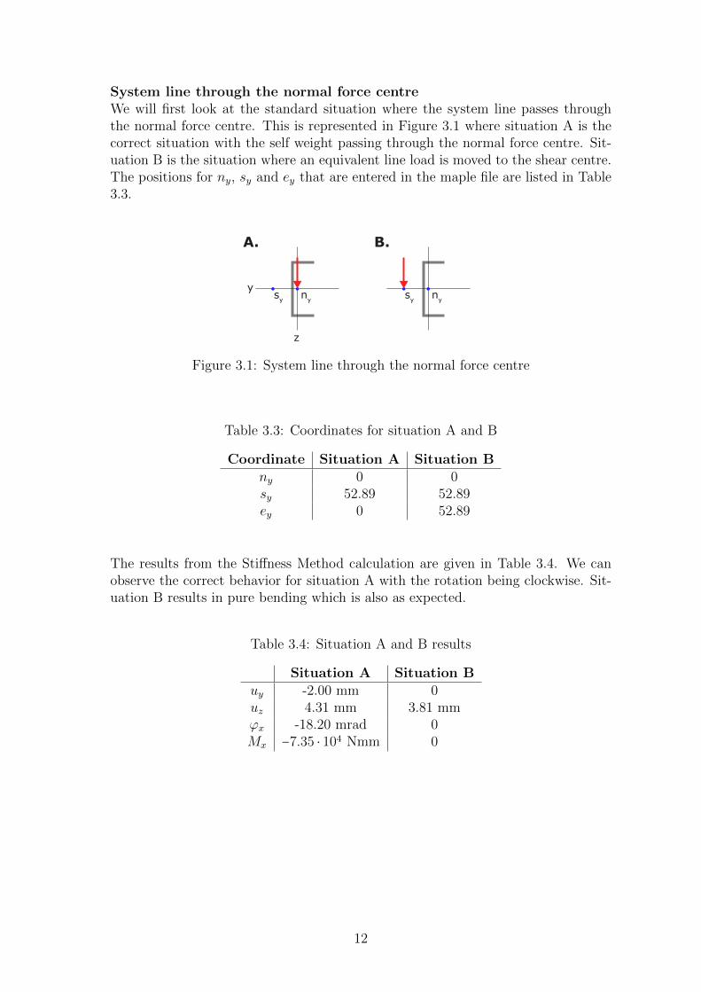
System line through the normal force centreWe will first look at the standard situation where the system line passes throughthe normal force centre. This is represented in Figure 3.1 where situation A is thecorrect situation with the self weight passing through the normal force centre. Sit-uation B is the situation where an equivalent line load is moved to the shear centre.The positions for ny, sy and ey that are entered in the maple file are listed in Table3.3.

z

y

B.

nysy

A.

nysy

Figure 3.1: System line through the normal force centre

Table 3.3: Coordinates for situation A and B

Coordinate Situation A Situation Bny 0 0sy 52.89 52.89ey 0 52.89

The results from the Stiffness Method calculation are given in Table 3.4. We canobserve the correct behavior for situation A with the rotation being clockwise. Sit-uation B results in pure bending which is also as expected.

Table 3.4: Situation A and B results

Situation A Situation Buy -2.00 mm 0uz 4.31 mm 3.81 mmϕx -18.20 mrad 0Mx −7.35 ⋅ 104 Nmm 0

12

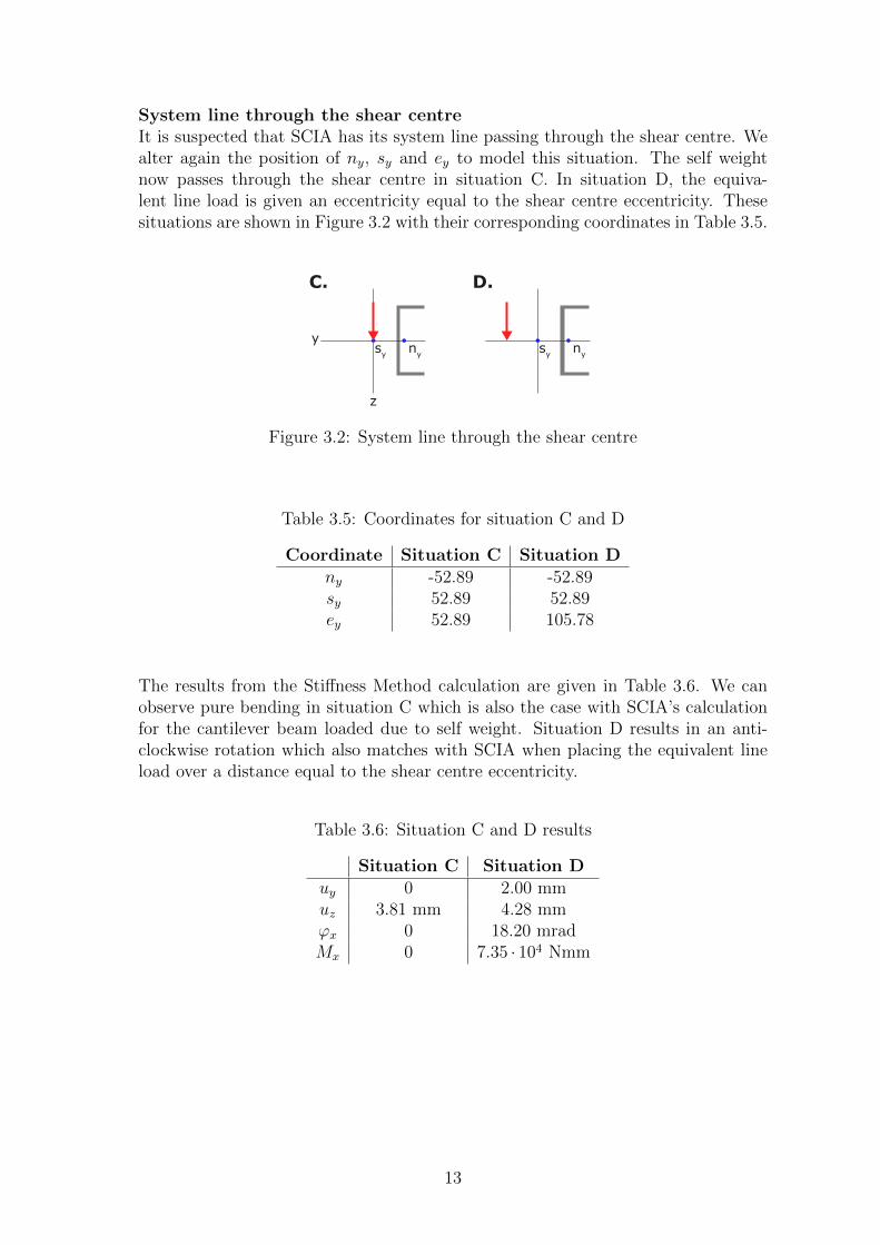
System line through the shear centreIt is suspected that SCIA has its system line passing through the shear centre. Wealter again the position of ny, sy and ey to model this situation. The self weightnow passes through the shear centre in situation C. In situation D, the equiva-lent line load is given an eccentricity equal to the shear centre eccentricity. Thesesituations are shown in Figure 3.2 with their corresponding coordinates in Table 3.5.

D.

nysy

z

y

C.

nysy

Figure 3.2: System line through the shear centre

Table 3.5: Coordinates for situation C and D

Coordinate Situation C Situation Dny -52.89 -52.89sy 52.89 52.89ey 52.89 105.78

The results from the Stiffness Method calculation are given in Table 3.6. We canobserve pure bending in situation C which is also the case with SCIA’s calculationfor the cantilever beam loaded due to self weight. Situation D results in an anti-clockwise rotation which also matches with SCIA when placing the equivalent lineload over a distance equal to the shear centre eccentricity.

Table 3.6: Situation C and D results

Situation C Situation Duy 0 2.00 mmuz 3.81 mm 4.28 mmϕx 0 18.20 mradMx 0 7.35 ⋅ 104 Nmm

13

Load to the right of the shear centreIt is likely that the problem in SCIA originates from the position of the system line.We can do one final check by placing the load on the other side of the shear centreand compare the results with SCIA’s output. This situation, situation E, is shownin Figure 3.3. The corresponding coordinates are listed in Table 3.7.

E.

nysy

z

y

Figure 3.3: System line through the shear centre

Table 3.7: Coordinates for situation E

Coordinate Situation Eny -52.89sy 52.89ey 0

We place the equivalent line load in SCIA to the right of the shear centre and reportthe results for the upper left fibre (point B in Figure 1.1). Comparing the result withsituation E shows that they are almost equal. The value for the vertical displacementfrom SCIA is shown in Figure 3.43 with the upper left fibre called ’Linksboven’.

Table 3.8: Situation E and SCIA

Situation E SCIAuy -2.00 mm -2.01 mmuz 3.34 mm 3.39 mmϕx -18.20 mrad -18.20 mradMx −7.35 ⋅ 104 Nmm −7.35 ⋅ 104 Nmm

Figure 3.4: Tabulated results in SCIA

3Note that some signs are different in this table, this has to do with SCIA’s sign convention. Anegative vertical displacement is for instance downwards.

14

3.3 Conclusion

SCIA assumes that the system line passes through the shear centre which is remark-able, but theoretically not incorrect. Engineers who know this, could take it intoaccount when working with the software. However, SCIA makes the self weight passthrough the shear centre as well. This is probably a mistake caused by the definitionof the system line. The error will stay unnoticed if the self weight is small in relationto the loading.

When a beam is assumed to be loaded in the shear centre, it is actually loadedwith an offset from the shear centre. This is why the equivalent line load appliedat a distance equal to the shear centre eccentricity results in torsion (situation D),whereas pure bending is expected (situation C). To compensate for the error, theoption ’consider torsion due to shear centre eccentricity’ can be enabled which is apost-processing fix.

15

Chapter 4

Safety

Now that we know more about the shear centre eccentricity error in SCIA andits possible solution, one question remains: could there be a potentially dangeroussituation in the future if the error is not fixed?

4.1 Dangers

There are two problems that arise with the error:

• SCIA only reports pure bending when there is an eccentricity of the shearcentre.

This can be potentially dangerous, because torsional moments can lead to highstresses. Also, the axial rotation will increase the deflection for some parts ofthe system. If there is an unity check with little capacity left then this couldbe exceeded due to the extra displacement. In case of the channel section inthis thesis, the increase in vertical displacement was more than 10 percentalongside horizontal displacement which was not present at all in case of purebending.

• Torsional stresses are only reported with the option ’consider torsion due toshear centre eccentricity’ enabled.

One of the biggest issues comes with the shear stresses. In Appendix A.2 theshear stresses are elaborated for the channel section. Here we can see that thetorsional shear stresses at the flanges are almost seventeen times bigger thanthe shear stresses due to the shear force. These stresses will increase with anincrease in shear force, but the torsional shear stresses then also increase. Thiscan definitely be problematic as the shear stresses are now much higher thanexpected which decreases the section’s shear capacity. Although enabling theoption ’consider torsion due to shear centre eccentricity’ will return correctresults, the button itself can be easily overlooked.

Apart form the problems mentioned above, showing the incorrect behavior for asystem with shear centre eccentricity is a bit careless as students and engineers whowork with the program can misinterpret the output.

16

4.2 Practical examples

Asymmetrical cross-sections or cross-sections with one axis of symmetry like chan-nel sections are not encountered as often as symmetrical cross-section like I-beams.In addition, those cross-sections are most of the time not loaded in torsion or onlysubjected to low loading. Because of these reasons, the chances of a structure failingdue to the error in SCIA are exceptionally low. A few examples of locations wherethese cross-sections can be encountered are purlins and staircases.

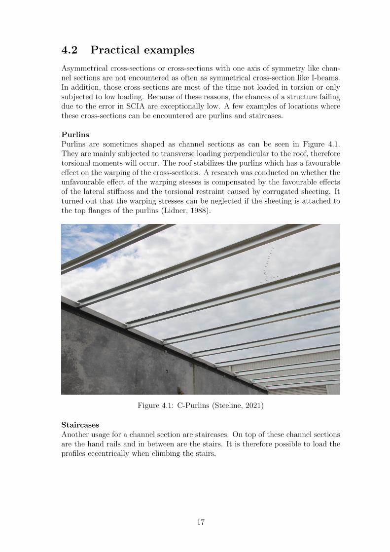
PurlinsPurlins are sometimes shaped as channel sections as can be seen in Figure 4.1.They are mainly subjected to transverse loading perpendicular to the roof, thereforetorsional moments will occur. The roof stabilizes the purlins which has a favourableeffect on the warping of the cross-sections. A research was conducted on whether theunfavourable effect of the warping stesses is compensated by the favourable effectsof the lateral stiffness and the torsional restraint caused by corrugated sheeting. Itturned out that the warping stresses can be neglected if the sheeting is attached tothe top flanges of the purlins (Lidner, 1988).

Figure 4.1: C-Purlins (Steeline, 2021)

StaircasesAnother usage for a channel section are staircases. On top of these channel sectionsare the hand rails and in between are the stairs. It is therefore possible to load theprofiles eccentrically when climbing the stairs.

17

Figure 4.2: Staircase at the TU Delft Faculty of Architecture

Figure 4.2 gives an example of a staircase with channel sections. There are no realstairs in this figure, it is a ramp used for fire emergencies. The bottom beams ofthis ramp are also made out of channel sections with their backs towards the stairs.The channel sections are supported at continuous intervals and welded all aroundresulting in a fixed connection. Therefore, the effect of torsion due to shear centreeccentricity is again small.

4.3 Conclusion

The chances of coming across a situation where asymmetrical cross-sections or cross-sections with one axis of symmetry are loaded in such a way that they become unsafeare low. These profiles can for example be encountered in purlins and staircases.SICA’s calculation error will therefore most likely not cause any dangerous situa-tions.

18

Chapter 5

Conclusion and recommendations

It was established that SCIA Engineer calculates no torsion if a cross-section hasa shear centre eccentricity. Drillenburg investigated this problem in 2017 by con-sidering different boundary conditions and load cases. We looked specifically at acantilever beam with a channel section loaded due to its self weight (Figure 1.1) inorder to figure out how the error could possibly be fixed.

5.1 Calculation comparison

We compared hand calculations with SCIA and Ansys Workbench, summarized theresults in tables and concluded the following:

• The results of Ansys match with the expectations, but the magnitudes of thedisplacements and rotations differ slightly from the hand calculation. This canbe explained by the use of slightly different torsional constant.

• SCIA reports no torsional moment, rotation or horizontal displacement undernormal loading circumstances. When moving a line load to the shear centre,SCIA does calculate a torsional moment which is not the correct behavior.

• The option ’consider torsion due to shear centre eccentricity’ reports the cor-rect magnitudes for the torsional shear stresses for both statically determinateand indeterminate beams, therefore Drillenburgs statement about the optionnot working properly is at least not true for a channel section.

5.2 Solution using the Stiffness Method

SCIA uses stiffness matrices to link forces and moments to displacements and rota-tions. To investigate where the error arises within the program, we created a stiffnessmatrix for a 3D beam element that accounts for the shear centre eccentricity usingMaple. All the steps are carefully explained in Appendix B.1. With the use of thismodel we came to the following hypothesis:

”SCIA’s stiffness matrix is correct for a system line through the shear centre.”

19

By looking at different positions for the system line, normal force centre and shearcentre in the code, we concluded where the error originated from. In a normalsituation, the system line would pass through the normal force centre. The selfweight of the channel section will then result in torsion. By placing an equivalentline load in the shear centre, only pure bending will be observed. This is illustratedin Figure 5.1.

z

y

B.

nysy

A.

nysy

Figure 5.1: System line in the normal force centre

If SCIA assumes that the system line passes through the shear centre, situationsA and B will change to situation C and D in Figure 5.2. The self weight now actsthrough the shear centre resulting in pure bending. Situation D is obtained byapplying an equivalent line load at a distance equal to the shear centre eccentricity.

D.

nysy

z

y

C.

nysy

Figure 5.2: System line in the normal force centre

This assumption is remarkable, but theoretically not incorrect. Engineers who areaware of this, can take it into account when working with the software. Having theself weight act through the shear centre however, is a mistake. This error will stayunnoticed if the self weight is small in relation to the loading.

5.3 Recommendations

SCIAEven though the chances of encountering a situation were the error could be danger-ous are exceptionally low, it is better to avoid the risks. SCIA is therefore stronglyadvised to move the system line to the normal force centre to avoid confusion. Theself weight must also act through the normal force centre instead of through theshear centre. If this is implemented correctly, the post-processing option ’considertorsion due to shear centre eccentricity’ can be removed.

20

EngineersSpecial attention is asked for cross-sections with a shear centre eccentricity, likechannel sections. If a system line through the normal force centre is preferred, theoption ’consider torsion due to shear centre eccentricity’ can be enabled in the re-sults tab to display the correct torsional shear stresses.

Follow-up researchCalculations for buckling are always made using a system line that passes throughthe normal force centre. It was established that SCIA uses a system line that passesthrough the shear centre. This will have consequences regarding the constructionof the stiffness matrix for buckling. It is therefore strongly advised to check if thebuckling of profiles with a shear centre eccentricity is calculated correctly in SCIA.

21

Bibliography

Drillenburg, M. (2017). Torsion and shear stresses due to shear centre eccentricityin SCIA Engineer (Bachelor’s Thesis). Delft University of Technology.

Hartsuijker, C. (2016). Spanningen, vervormingen en verplaatsingen (2nd ed.).Boom uitgevers Amsterdam.

Hoogenboom, P. (2008). Aantekeningen over wringing. (pdf-edition)

James F. Lincoln Arc Welding Foundation. (2021). Torque equations. Retrievedfrom https://www.sprecace.com/node/61

Lidner, J. (1988). To the load carrying capacity of cold-formed purlins. MissouriUniversity of Science and Technology. (pdf-edition)

Moaveni, S. (2011). Finite element analysis theory and application with ANSYS(3rd ed.). Pearson. (table 4.2)

Steeline. (2021). Purlin-C. Retrieved from https://www.steeline.com.au/wp

-content/uploads/2019/03/IMG 6921-2000x1224.jpg

Welleman, H. (2021). Non-symmetrical and inhomogeneous cross sections. (pdf-edition)

Young, W. C., Budynas, R. G., & Sadegh, A. M. (2002). Roark’s formulas for stressand strain (7th ed.). McGraw-Hill Education. (pg. 407)

22

Appendices

23

Appendix A

Hand calculations

A.1 Cross-sectional properties

24

> >

> >

> >

> >

> >

> >

(2)(2)

> > (1)(1)

> >

Hand calculations

Roarks Method

Simplified approach (thin-walled)

> >

(6)(6)

> >

(5)(5)

(7)(7)

(4)(4)

> >

> >

> >

(9)(9)

(2)(2)

> >

> >

> >

(3)(3)

> >

(8)(8)

(10)(10)

> >

Cross-sectional properties

Normal force centre

0.

Shear centre

Loading, displacements and rotations

mm

(19)(19)

> >

> >

(14)(14)

> >

> >

> >

> >

(2)(2)

> >

> >

> >

(15)(15)

(18)(18)

(17)(17)

> >

(13)(13)

(11)(11)

(12)(12)

> >

(16)(16)

Torsional shear stress

mm2

mm2

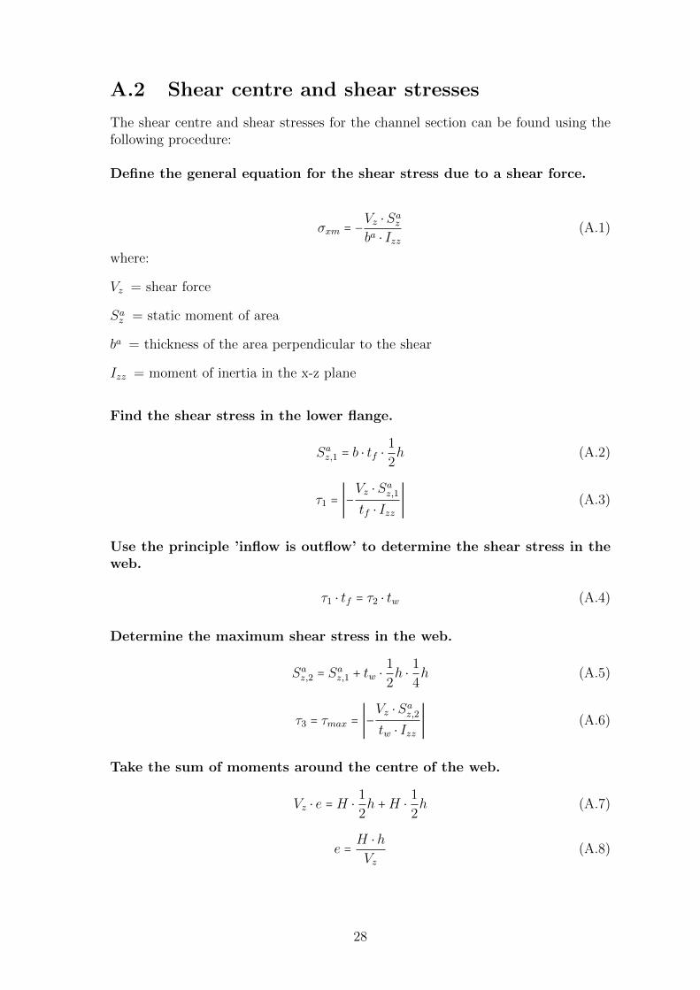
A.2 Shear centre and shear stresses

The shear centre and shear stresses for the channel section can be found using thefollowing procedure:

Define the general equation for the shear stress due to a shear force.

σxm = −Vz ⋅ Sa

z

ba ⋅ Izz(A.1)

where:

Vz = shear force

Saz = static moment of area

ba = thickness of the area perpendicular to the shear

Izz = moment of inertia in the x-z plane

Find the shear stress in the lower flange.

Saz,1 = b ⋅ tf ⋅

1

2h (A.2)

τ1 = ∣−Vz ⋅ Sa

z,1

tf ⋅ Izz∣ (A.3)

Use the principle ’inflow is outflow’ to determine the shear stress in theweb.

τ1 ⋅ tf = τ2 ⋅ tw (A.4)

Determine the maximum shear stress in the web.

Saz,2 = S

az,1 + tw ⋅

1

2h ⋅

1

4h (A.5)

τ3 = τmax = ∣−Vz ⋅ Sa

z,2

tw ⋅ Izz∣ (A.6)

Take the sum of moments around the centre of the web.

Vz ⋅ e =H ⋅1

2h +H ⋅

1

2h (A.7)

e =H ⋅ h

Vz(A.8)

28

Find H by combining Equation A.2 and A.3.The horizontal force H is equal to the area of the lower triangle in Figure A.1multiplied with the thickness.

τ1 = ∣−Vz ⋅ b ⋅

12h

Izz∣ (A.9)

H =1

2b ⋅ τ1 ⋅ tf =

1

4⋅VzIzz⋅ b2 ⋅ h ⋅ tf (A.10)

Combine Equation A.8 and A.10 to obtain the shear centre eccentricitywith respect to the centre of the web.

e =b2 ⋅ h2 ⋅ tf

4Izz(A.11)

Equation A.11 can also be used for a thick-walled channel section by accounting forthe thicknesses. The validation of this equation is left to the reader.

e =(b − tw

2 )2⋅ (h − tf)2 ⋅ tf

4Izz(A.12)

Torsional shear stressThe torsional shear stresses are assumed to be linear across the wall thickness. Themaximum torsional shear stress then occurs at 1

2t. Using this in combination withthe previously defined equations for the shear stress, the following equations areobtained for the maximum torsional shear stress:

τf ;max =Mt ⋅ tfIt

(A.13)

τw;max =Mt ⋅ twIt

(A.14)

The total maximum shear stress can be obtained by using the superposition prin-ciple: adding the torsional shear stress and the shear stress due to the shear force.It is important to note that the shear stress due to the shear force is assumed tobe constant across the wall thickness. In Figure A.1 τ1 is calculated using EquationA.3, τ2 is calculated using Equation A.4 and τ3 using Equation A.6.

29

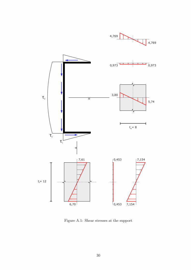
7,61

6,70

0,453

0,453 7,154

7,154

4,769

τ3

τ2

τ1

4,769

0,973 0,973

3,80

5,74

tw= 8

tf= 12

Figure A.1: Shear stresses at the support

30

Appendix B

Stiffness Method

B.1 Solution strategy

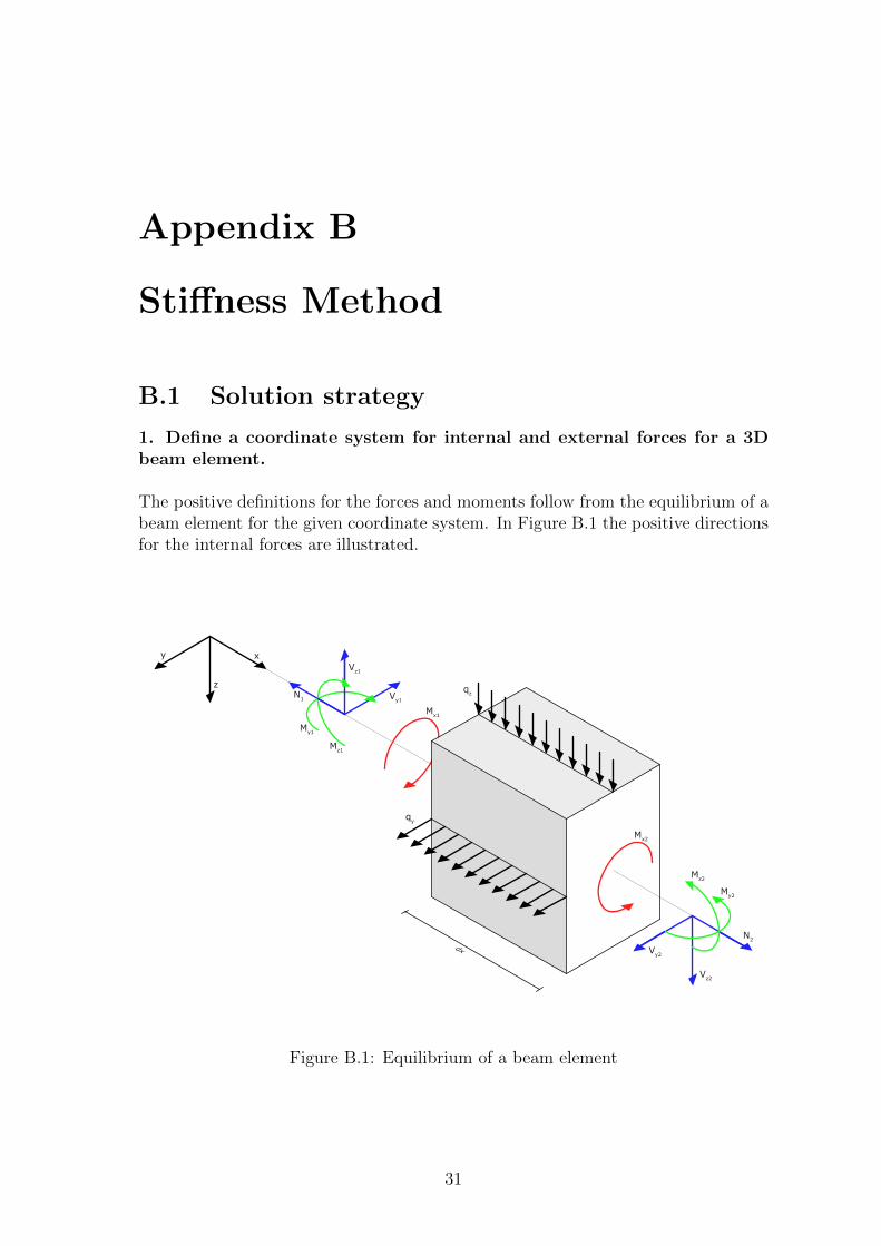
1. Define a coordinate system for internal and external forces for a 3Dbeam element.

The positive definitions for the forces and moments follow from the equilibrium of abeam element for the given coordinate system. In Figure B.1 the positive directionsfor the internal forces are illustrated.

xy

zN1

N2

Vy1

Mx1

qz

qy

Mx2

Vy2

Vz1

Vz2

My1

My2

Mz1

Mz2

Figure B.1: Equilibrium of a beam element

31

2. Define the equations for the beam properties.

ElongationThe elongation of the beam is defined as the change of displacement in x-direction.

e =duxdx

(B.1)

CurvaturesThe curvatures of the beam in y- and z-direction are defined as the change in rotationin the y- and z-direction.

κy = −dϕy

dx(B.2)

κz = −dϕz

dx(B.3)

Forces and Moments

N = EA ⋅ e +EA ⋅ ny ⋅ κy +EA ⋅ nz ⋅ κz (B.4)

My = EA ⋅ ny ⋅ e +EIyy ⋅ κy +EIyz ⋅ κz (B.5)

Mz = EA ⋅ nz ⋅ e +EIyz ⋅ κy +EIzz ⋅ κz (B.6)

Mx = GIt ⋅dϕx

dx(B.7)

Vy =dMy

dx(B.8)

Vz =dMz

dx(B.9)

3. Set up the differential equations and boundary conditions.

Differential Equations

dN

dx= 0 (B.10)

d2My

dx2= 0 (B.11)

d2Mz

dx2= 0 (B.12)

32

d2Mx

dx2= 0 (B.13)

ϕy −duydx= 0 (B.14)

ϕz −duzdx= 0 (B.15)

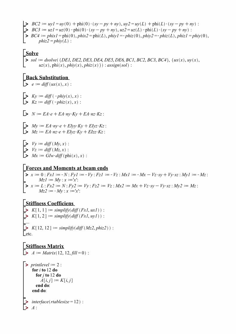
Boundary Conditionsny and nz are the coordinates of the normal force centre, sy and sz are the coordi-nates of the shear centre with respect to the normal force centre and py and pz arethe coordinates of a point on the cross-section.

U =

⎧⎪⎪⎪⎪⎪⎪⎪⎪⎪⎪⎪⎪⎪⎨⎪⎪⎪⎪⎪⎪⎪⎪⎪⎪⎪⎪⎪⎩

ux1 = ux(0)

ux2 = ux(L)

uy1 = uy(0) + ϕx(0) ⋅ (sz − pz + nz)

uy2 = uy(L) + ϕx(L) ⋅ (sz − pz + nz)

uz1 = uz(0) − ϕx(0) ⋅ (sy − py + ny)

uz2 = uz(L) − ϕx(L) ⋅ (sy − py + ny)

(B.16)

Φ =

⎧⎪⎪⎪⎪⎪⎪⎪⎪⎪⎪⎪⎪⎪⎨⎪⎪⎪⎪⎪⎪⎪⎪⎪⎪⎪⎪⎪⎩

ϕx1 = ϕx(0)

ϕx2 = ϕx(L)

ϕy1 = −ϕz(0)

ϕy2 = −ϕz(L)

ϕz1 = ϕy(0)

ϕz2 = ϕy(L)

(B.17)

4. Solve the system.

Solving the system results in expressions for the displacements and rotations asfunctions of x.

5. Substitute the solution back into the previously defined equations.

The results from step 4 are substituted back into the equations from step 2.

33

6. Set up the forces and moments on both ends of the beam element.The forces and moments in the nodes are according to the positive directions inFigure B.1.

F1 =

⎧⎪⎪⎪⎪⎪⎪⎪⎪⎪⎪⎪⎪⎪⎨⎪⎪⎪⎪⎪⎪⎪⎪⎪⎪⎪⎪⎪⎩

Fx1 = −N

Fy1 = −Vy

Fz1 = −Vz

Mx1 = −Mx − Vz ⋅ sy + Vy ⋅ sz

My1 = −Mz

Mz1 =My

(B.18)

F2 =

⎧⎪⎪⎪⎪⎪⎪⎪⎪⎪⎪⎪⎪⎪⎨⎪⎪⎪⎪⎪⎪⎪⎪⎪⎪⎪⎪⎪⎩

Fx2 = N

Fy2 = Vy

Fz2 = Vz

Mx2 =Mx + Vz ⋅ sy − Vy ⋅ sz

My2 =Mz

Mz2 = −My

(B.19)

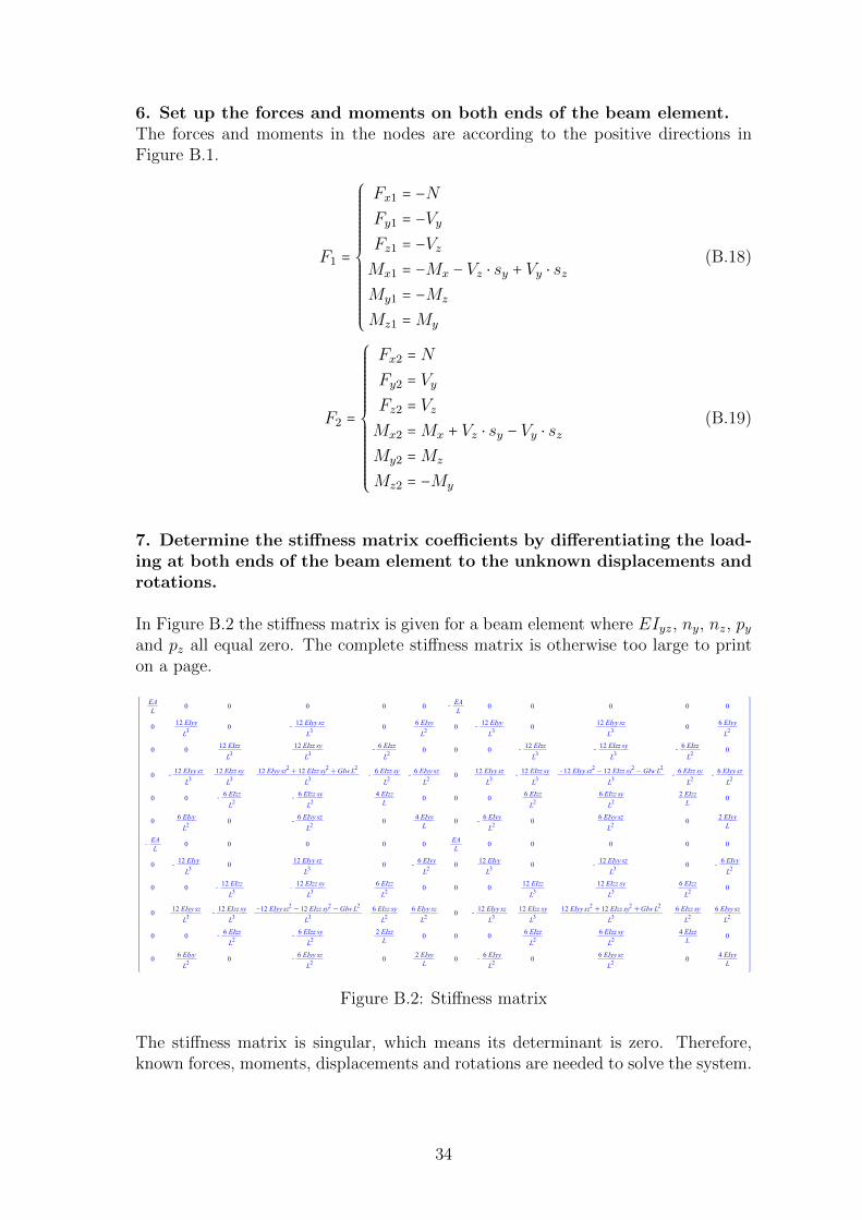
7. Determine the stiffness matrix coefficients by differentiating the load-ing at both ends of the beam element to the unknown displacements androtations.

In Figure B.2 the stiffness matrix is given for a beam element where EIyz, ny, nz, pyand pz all equal zero. The complete stiffness matrix is otherwise too large to printon a page.

Figure B.2: Stiffness matrix

The stiffness matrix is singular, which means its determinant is zero. Therefore,known forces, moments, displacements and rotations are needed to solve the system.

34

8. Solve the system for the unknown displacements and rotations by ap-plying known forces, moments, displacements and rotations.

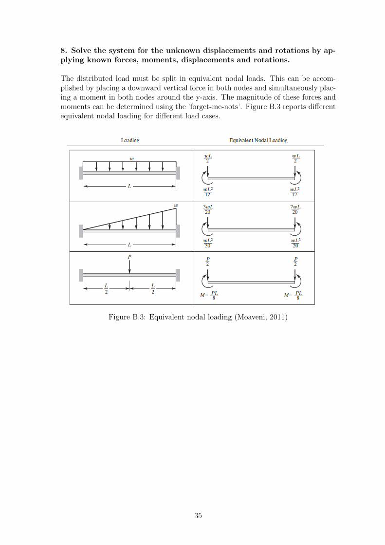
The distributed load must be split in equivalent nodal loads. This can be accom-plished by placing a downward vertical force in both nodes and simultaneously plac-ing a moment in both nodes around the y-axis. The magnitude of these forces andmoments can be determined using the ’forget-me-nots’. Figure B.3 reports differentequivalent nodal loading for different load cases.

Figure B.3: Equivalent nodal loading (Moaveni, 2011)

35

B.2 Maple file - hand calculation properties

36

> >

> >

> >

> >

> >

> >

> >

> > > >

> >

> >

> >

> >

> >

> >

> >

> >

(properties: hand calculation)

Beam Equations

Differential Equations

Boundary Conditions

> >

> >

> >

> >

> >

> >

> >

> >

> >

> >

> >

> >

> >

> >

> >

> >

> >

> >

> >

> >

> >

> >

Solve

Back Substitution

Forces and Moments at beam ends

Stiffness Coefficiens

...

etc.

Stiffness Matrix

> >

> >

> >

(1)(1)

> >

> >

> >

> >

> >

> >

> >

Parameters (hand calculation)

Loading

Solution

B.3 Maple file - SCIA properties

40

> >

> >

> >

> >

> >

> >

> >

> >

> >

> >

> >

> >

> >

> >

> >

> >

(properties: SCIA, situation E)

Beam Equations

Differential Equations

> >

> >

> >

> >

> >

> >

> >

> >

> >

> >

> >

> >

> >

> >

> >

> >

> >

> >

> >

> >

> >

Boundary Conditions

Solve

Back Substitution

Forces and Moments at beam ends

Stiffness Coefficiens

...

etc.

Stiffness Matrix

> >

> >

> >

> >

> >

> >

> >

> >

> >

> >

> >

(1)(1)

Parameters (hand calculation)

Loading

Solution