SHARP PROPAGATION OF CHAOS ESTIMATES FORFEYNMAN-KAC PARTICLE MODELS

PIERRE DEL MORAL∗, ARNAUD DOUCET† , GARETH W. PETERS†

Abstract. This article is concerned with the propagation-of-chaos properties of genetic typeparticle models. This class of models arises in a variety of scientific disciplines including theoreticalphysics, macromolecular biology, engineering sciences, and more particularly in computational statis-tics and advanced signal processing. From the pure mathematical point of view, these interactingparticle systems can be regarded as a mean field particle interpretation of a class of Feynman-Kacmeasures on path spaces.

In the present article, we design an original integration theory of propagation-of-chaos basedon the fluctuation analysis of a class of interacting particle random fields. We provide analyticfunctional representations of the distributions of finite particle blocks, yielding what seems to be thefirst result of this kind for interacting particle systems. These asymptotic expansions are expressedin terms of the limiting Feynman-Kac semigroups and a class of interacting jump operators. Theseresults provide both sharp estimates of the negligible bias introduced by the interaction mechanisms,and central limit theorems for nondegenerate U -statistics and von Mises statistics associated withgenealogical tree models. Applications to nonlinear filtering problems and interacting Markov chainMonte Carlo algorithms are discussed.

Key words. Interacting particle systems, historical and genealogical tree models, propagation-of-chaos, central limit theorems, Gaussian fields.

AMS subject classifications. 60F17, 60K35, 60J25, 65C05, 65D30, 60J75, 60G44, 60F05,60G35

1. Introduction. In this article, we present an original fluctuation analysis ofthe propagation of chaos properties of a class of genetic type interacting particle sys-tems. This subject has various natural links to statistical physics, macromolecularbiology, engineering sciences, and more particularly, to rare event estimation, nonlin-ear filtering, global optimization, and sequential Monte Carlo theory.

The objects on which these particle models are sought vary considerably from oneapplication area to another. But, from the strict mathematical and physical point ofview, the genetic models discussed in this study can be interpreted as mean field par-ticle approximations of an abstract and general class of Feynman-Kac path-measures.From the point of view of statistics and engineering sciences, these models can alsobe interpreted as methods to sample from complex distributions on path spaces. Inobserving this connection, we mention that the propagation of chaos properties ofinteracting processes allows us to measure the statistical bias, as well as the degreeof independence between the sampled particles. For a detailed review of these modelapplication areas, and precise asymptotic theory of these particle schemes, we referthe reader to the recent research books of the first and second authors [2, 7].

The study of the propagations of chaos properties for discrete and continuoustime genetic models was begun in [5, 6], and it has been further developed in [2].These three studies have been influenced by the article of G. Ben Arous and O.I.Zeitouni [1], and the pioneering studies of C. Graham and S. Meleard [8], and S.Meleard [11]. In the articles [1, 5], increasing propagation of chaos properties are dis-cussed for McKean-Vlasov diffusions, as well as for genetic type particle models with

∗Laboratoire J. A. Dieudonne, Departement de Mathematiques, Universite de Nice Sophia-Antipolis, Parc Valrose, 06 108 Nice, France. Email: delmoral@math.unice.fr

†Information Engineering Division, Engineering Department, Cambridge University, Trumping-ton Street, CB2 1PZ Cambridge, UK. Email: {ad2,gwp20}@eng.cam.ac.uk

1

sufficiently regular mutation transitions. We note that the change of reference mea-sure technique, developed in [5], relies entirely on some regularity conditions on themutation transition, which are not satisfied for path-particle models. As a result, theydo not apply to genealogical particle tree models. In the articles [8, 11], the authorspresent strong propagation of chaos results for the N -particle approximating modelassociated with a class of generalized Boltzmann equations. Using general interactinggraphs and precise coupling techniques, they show that the order of convergence forthe total variation distance between the law of the q-first particles and the limiting dis-tribution on a compact interval [0, t] is q2 c(t)/N . The connections between spatiallyhomogeneous Boltzmann equations and continuous time Feynman-Kac formulae aredescribed in some detail in [2, 6]. Loosely speaking, the microscopic colliding particleinterpretations of the generalized Boltzmann equations introduced by S. Meleard [11]can also be interpreted as selective interacting jump models. In the articles [2, 5, 6],the authors have also obtained, in the context of genetic models, the same increasingpropagation of chaos property using an alternative original Feynman-Kac semigroupapproach.

The increasing propagation of chaos property developed in the above series ofarticles leads us inevitably to question the sharpness of the order q2/N . Furthermore,in most of these studies, the remainder control constant c(t) increases exponentiallyfast to infinity, as the time parameter increases. As a consequence, these estimatescannot really be used in practice to quantify the degree of independence, and theperformance of the particle interpretation models.

The increasing propagation of chaos properties discussed in this paper show thatthe order q2/N is actually sharp. Additionally, we derive precise asymptotic expan-sions of the law of finite particle blocks with respect to the size of the system. Ouranalysis does not rely on any regularity condition on the mutation transitions. Con-sequently, it applies to path space genealogical tree models. In contrast to traditionalstudies on this theme, our approach also describes the precise fluctuations associatedwith these asymptotic weak expansions. From a statistical point of view, these fluc-tuations can be interpreted as central limit theorems for nondegenerate U -statistics.These results extend the original central limit theorem for U -statistics due to Hoeffd-ing [9, 10] for independent and identically distributed random variables to mean fieldand genealogical processes. Moreover, we provide a semigroup technique to estimatethe first order operator of these asymptotic expansions. For sufficiently regular mod-els, we show that the asymptotic remainder constant c(t) is uniformly bounded withrespect to the time parameter.

The rest of this article is organized as follows:In a preliminary section, Subsection 1.1, we provide a mathematical description

of the Feynman-Kac models and their probabilistic particle interpretations.In Subsection 1.2, we describe our main results. We start with a brief reminder

of the propagation of chaos properties of interacting particle systems. Then we de-velop an asymptotic propagation of chaos estimate for polynomial tensor product testfunctions. This first result applies to a general class of particle McKean interpreta-tion models on abstract measurable state spaces. We already mentioned that thisresult also provides a sharp estimate of the bias introduced by the particle interactionmechanisms. In the second part, we extend this propagation of chaos property to thecontext of simple genetic models on locally compact and separable metric spaces. Weprovide a first order asymptotic expansion of the distribution of finite particle blocks.

In Subsection 1.3, we illustrate this abstract class of models with two concrete2

scenarios arising in applied probability, computational statistics and engineering sci-ences. In the first scenario, we discuss a class of interacting Markov chain MonteCarlo algorithms to sample from complex high dimensional distributions and to sam-ple paths of Markov chains restricted to their terminal values. These particle models,also known as Sequential Monte Carlo samplers, were recently introduced by the firsttwo authors [3]. Their applications to statistics and global optimization were furtherdeveloped in a joint work with the third author [4]. The second scenario described inthis section is related to nonlinear filtering problems. This class of Feynman-Kac typemodels are currently used in advanced signal processing and Bayesian analysis. Inthis context, the corresponding genetic particle approximation models are also knownas particle filters. In both situations, it is essential to estimate the bias induced by theinteraction mechanisms, as well as the degree of independence between the particles.The asymptotic propagation of chaos expansions developed in this article provideprecise answers to these two fundamental questions.

In Section 2 we have collected a series of results on both the weak convergenceof random fields, and on the combinatorial transport properties of q-tensor productparticle measures. Section 3 presents the proof of the main results of this article. Inthe final section, Section 4, we present an original semigroup contraction techniqueto control the first order operator of the asymptotic propagation of chaos expansionuniformly in time.

1.1. Description of the models. Let (En, En)n≥0 be a collection of measurablestate spaces, and denote by Bb(En) the Banach space of all bounded and measurablefunctions f on En, equipped with the uniform norm ‖f‖ = supxn∈En

|f(xn)|. We alsoconsider a collection of potential functions Gn on the state spaces En, a distributionη0 on E0, and a collection of Markov transitions Mn(xn−1, dxn) from En−1 into En.To simplify the presentation, and avoid unnecessary technical discussion, we shallsuppose that the potential functions are chosen such that

sup(xn,x′n)∈E2

n

Gn(xn)/Gn(x′n) < ∞.

We associate the Feynman-Kac measures, defined for any fn ∈ Bb(En) by the formulae

ηn(fn) = γn(fn)/γn(1) with γn(fn) = E[fn(Xn)∏

0≤k<n Gk(Xk)] (1.1)

to the pair potentials/transitions (Gn,Mn). In (1.1), (Xn)n≥0 represents a Markovchain with initial distribution η0, and elementary transitions Mn.

The advantage of the general Feynman-Kac model presented here is that it uni-fies the theoretical analysis of a variety of genetic type algorithms currently used inBayesian statistics, biology, particle physics, and engineering sciences. It is clearlyout of the scope of this article to present a detailed review of these particle approx-imation models. We rather refer the reader to the pair of research books [2, 7], andreferences therein. To illustrate this rather abstract model, two concrete applicationsare discussed in some details in section 1.3.

It is important to notice that this abstract formulation is particularly useful fordescribing Markov motions on path spaces. For instance, Xn may represent thehistorical process

Xn = (X ′0, . . . , X

′n) ∈ En = E′

[0,n] = E′0 × . . .× E′

n (1.2)

associated with an auxiliary Markov chain X ′n which takes values in some measurable

state spaces E′n. As we shall see, this apparently innocent observation is particularly

3

useful for modelling and analyzing genealogical evolution processes. By the Markovproperty and the multiplicative structure of (1.1), it is easily checked that the flow(ηn)n≥0 satisfies the following equation

ηn+1 = Ψn(ηn)Mn+1 =def.

∫En

Ψn(ηn)(dxn) Mn+1(xn, .) (1.3)

where the Boltzmann-Gibbs transformation Ψn is defined by

Ψn(ηn)(dxn) =1

ηn(Gn)Gn(xn) ηn(dxn).

The particle approximation of the flow (1.3) depends on the choice of the McKeaninterpretation model. These probabilistic interpretations consist of a chosen collectionof Markov transitions Kn+1,ηn

, indexed by the set of probability measures ηn on En,and satisfying the compatibility condition

Ψn(ηn)Mn+1 = ηnKn+1,ηn(=∫

ηn(dxn)Kn+1,ηn(xn, .)).

These collections are not unique. We can choose, for instance, Kn+1,ηn= Sn,ηn

Mn+1,where Sn,ηn

(xn, dyn) is the updating Markov transition on En defined by

Sn,ηn(xn, dyn) = εnGn(xn) δxn

(dyn) + (1− εnGn(xn)) Ψn(ηn)(dyn) (1.4)

In the above formula, εn represents any (possibly null) constant such that ‖εnGn‖ ≤ 1.The corresponding nonlinear equation

ηn+1 = ηnKn+1,ηn

can be interpreted as the evolution of the law of the states of a canonical Markovchain Xn whose elementary transitions Kn+1,ηn depend on the law of the currentstate. That is, we have that

P(Xn+1 ∈ dxn+1 | Xn = xn) = Kn+1,ηn(xn, dxn+1) with P ◦X−1

n = ηn (1.5)

The law Pn of the random canonical path (Xp)0≤p≤n under the McKean measure Pis simply defined by

Pn(d(x0, . . . , xn)) = η0(dx0) K1,η0(x0, dx1) . . . Kn,ηn−1(xn−1, dxn)

The mean field particle model associated with such McKean model is an ENn -

valued Markov chain ξ(N)n = (ξ(N,i)

n )1≤i≤N with elementary transitions defined insymbolic form by

P(ξ(N)n ∈ d(x1

n, . . . , xNn ) | ξ

(N,i)n−1 ) =

N∏i=1

Kn,ηNn−1

(ξ(N,i)n−1 , dxi

n) (1.6)

with the empirical N particles measures

ηNn−1 =def.

1N

N∑j=1

δξ(N,j)n−1

4

In formula above d(x1n, . . . , xN

n ) represents an infinitesimal neighborhood of the point(x1

n, . . . , xNn ) ∈ EN

n . The initial configuration ξ(N)0 = (ξ(N,i)

0 )1≤i≤N consists of Nindependent and identically distributed random variables with distribution η0. Asusual, when there is no possible confusion, we simplify notation and suppress theindex (.)(N) and write (ξn, ξi

n) instead of (ξ(N)n , ξ

(N,i)n ).

By the definition of the McKean transitions it appears that (1.6) is the com-bination of simple selection/mutation genetic transitions. The selection stage con-sists of N randomly evolving path-particles ξi

n−1 ξin−1 according to the update

transition Sn,ηNn−1

(ξin−1, .). In other words, with probability εn−1Gn−1(ξi

n−1), we set

ξin−1 = ξi

n−1; otherwise, the particle jumps to a new location, randomly drawn fromthe discrete distribution Ψn−1(ηN

n−1). During the mutation stage, each of the selectedparticles ξi

n−1 ξin evolves according to the Markov transition Mn.

If we consider the historical process Xn = (X ′0, . . . , X

′n) introduced in (1.2), then

the above mean field model consists of N path particles evolving according to thesame selection/mutation transitions. It is immediately clear that the resulting particlemodel can be interpreted as the evolution of a genealogical tree model. Also noticethat for ε = 0, the particle interpretation model reduces to a simple mutation/selectiongenetic model.

It is obviously out of the scope of this article to present a full asymptotic analysisof these genealogical particle models. We refer the interested reader to the recentresearch monograph [2], and the references therein. For instance, it is well knownthat the occupation measures of the ancestral lines converge to the desired Feynman-Kac measures. That is, we have with various precision estimates, and as N tends toinfinity, the weak convergence result limN→∞ ηN

n = ηn.

1.2. Statement of main results. Several propagation of chaos estimates havebeen recently obtained which ensure that the particles ξi

n are asymptotically indepen-dent and identically distributed with common distribution ηn. The weakest form ofthis property can be stated as follows. We say that the particle model ξn = (ξi

n)1≤i≤N

is weakly chaotic with respect to the measure ηn if we have

limN→∞

E

(q∏

i=1

f (i)n (ξi

n)

)=

q∏i=1

ηn(f (i)n ) (1.7)

for any finite block size q ≤ N , any time horizon, and any sequence of functions(f (i)

n )1≤i≤q ∈ Bb(Eqn). This propagation of chaos property is known to be satisfied

for the McKean interpretation models defined in (1.4). Note that if q = 1 then (1.7)simply says that the law of a single particle is asymptotically unbiased. In otherwords, by the exchangeability property of the particle model we have that

E(f (1)n (ξ1

n)) = E(ηNn (f (1)

n )) → ηn(f (1)n ) as N →∞. (1.8)

If we take ε = 0 in (1.4), the particle model reduces to a simple genetic model.In this context, we also have the increasing propagation of chaos estimate

‖Law(ξ1n, . . . , ξq

n)− η⊗qn ‖tv ≤ c(n) q2/N (1.9)

for some finite constant, which only depends on the time parameter n and where ‖.‖tvdenotes the total variation norm on the set of bounded measures. The complete proofof this well-known result, and related estimates with respect to relative entropy type

5

criteria, can be founded in [2] (see for instance the theorems 8.3.2, and 8.3.3, on pp.259-260).

The main object of this article is to provide an asymptotic functional expansion ofthese two convergence results with respect to the precision parameter N . To simplifythe presentation, we shall often use the following slight abuse of notation; for a givenMarkov transition K from a measurable space (E, E) into another space (F,F), andfor any pair of functions f, g ∈ Bb(F ), we write

K[(f −K(f))(g −K(g))](x) =def.K[(f −K(f)(x))(g −K(g)(x))](x)= K(fg)(x)−K(f)(x)K(g)(x)

Our asymptotic expansions are expressed in terms of a collection of independent andcentered Gaussian fields Wn on the Banach function spaces Bb(En); with for anyfn, gn ∈ Bb(En),

E(Wn(fn)Wn(gn)) = ηn−1Kn,ηn−1([fn −Kn,ηn−1(fn)][gn −Kn,ηn−1(gn)]) (1.10)

For n = 0 we use the convention K0,η−1 = η0. The Gaussian fields Wn represent theasymptotic fluctuations of the local sampling errors associated with the mean fieldparticle approximation sampling steps. To describe precisely our first main result,we let Qp,n, with 0 ≤ p ≤ n, be the Feynman-Kac semi-group associated with theflow γn = γpQp,n. For p = n, we use the convention that Qn,n = Id. Using theMarkov property, it is not difficult to check that Qp,n has the following functionalrepresentation

Qp,n(fn)(xp) = E[fn(Xn)

∏p≤k<n Gk(Xk) | Xp = xp

](1.11)

for any test function fn ∈ Bb(En), and any state xp ∈ Ep. To check this assertion, wesimply note that

γn(fn) = E

[∏

0≤k<p

Gk(Xk)]× E

fn(Xn)∏

p≤k<n

Gk(Xk) | (X0, . . . , Xp)

= E

[∏

0≤k<p

Gk(Xk)] Qp,n(fn)(Xp)

= γpQp,n(fn)

which establishes (1.11). For p = n we use the convention∏∅ = 1 and Qp,n = Id.

We also denote by Rp,n the renormalized semigroup from Ep into En given by

Rp,n(fn) =Qp,n(fn)

ηp(Qp,n(1))=

γp(1)γn(1)

Qp,n(fn) (1.12)

Theorem 1.1. For any time horizon n ≥ 0, any block size parameter 0 < q ≤ N ,and every sequence of functions f

(k)n ∈ Bb(En), with ηn(f (k)

n ) = 1, and 1 ≤ k ≤ q, wehave

limN→∞

N E

[q∏

k=1

ηNn (f (k)

n )− 1

]

= −∑q

i=1

∑n−1p=0 γp(1)2 E

(Wp(Qp,n1) Wp(Qp,n[f (i)

n − 1]))

+∑

1≤i<j≤q

∑np=0 E

(Wp(Rp,n(f (i)

n − 1))Wp(Rp,n(f (j)n − 1))

)(1.13)

6

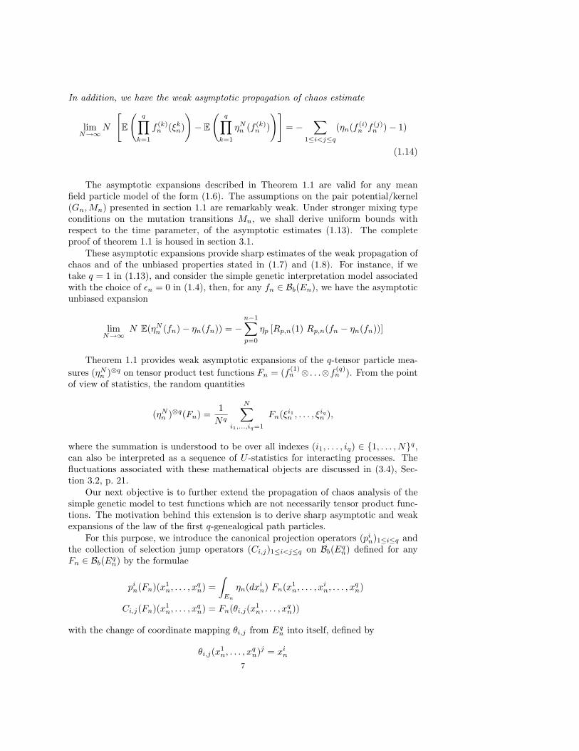
In addition, we have the weak asymptotic propagation of chaos estimate

limN→∞

N

[E

(q∏

k=1

f (k)n (ξk

n)

)− E

(q∏

k=1

ηNn (f (k)

n )

)]= −

∑1≤i<j≤q

(ηn(f (i)n f (j)

n )− 1)

(1.14)

The asymptotic expansions described in Theorem 1.1 are valid for any meanfield particle model of the form (1.6). The assumptions on the pair potential/kernel(Gn,Mn) presented in section 1.1 are remarkably weak. Under stronger mixing typeconditions on the mutation transitions Mn, we shall derive uniform bounds withrespect to the time parameter, of the asymptotic estimates (1.13). The completeproof of theorem 1.1 is housed in section 3.1.

These asymptotic expansions provide sharp estimates of the weak propagation ofchaos and of the unbiased properties stated in (1.7) and (1.8). For instance, if wetake q = 1 in (1.13), and consider the simple genetic interpretation model associatedwith the choice of εn = 0 in (1.4), then, for any fn ∈ Bb(En), we have the asymptoticunbiased expansion

limN→∞

N E(ηNn (fn)− ηn(fn)) = −

n−1∑p=0

ηp [Rp,n(1) Rp,n(fn − ηn(fn))]

Theorem 1.1 provides weak asymptotic expansions of the q-tensor particle mea-sures (ηN

n )⊗q on tensor product test functions Fn = (f (1)n ⊗ . . .⊗f

(q)n ). From the point

of view of statistics, the random quantities

(ηNn )⊗q(Fn) =

1Nq

N∑i1,...,iq=1

Fn(ξi1n , . . . , ξiq

n ),

where the summation is understood to be over all indexes (i1, . . . , iq) ∈ {1, . . . , N}q,can also be interpreted as a sequence of U -statistics for interacting processes. Thefluctuations associated with these mathematical objects are discussed in (3.4), Sec-tion 3.2, p. 21.

Our next objective is to further extend the propagation of chaos analysis of thesimple genetic model to test functions which are not necessarily tensor product func-tions. The motivation behind this extension is to derive sharp asymptotic and weakexpansions of the law of the first q-genealogical path particles.

For this purpose, we introduce the canonical projection operators (pin)1≤i≤q and

the collection of selection jump operators (Ci,j)1≤i<j≤q on Bb(Eqn) defined for any

Fn ∈ Bb(Eqn) by the formulae

pin(Fn)(x1

n, . . . , xqn) =

∫En

ηn(dxin) Fn(x1

n, . . . , xin, . . . , xq

n)

Ci,j(Fn)(x1n, . . . , xq

n) = Fn(θi,j(x1n, . . . , xq

n))

with the change of coordinate mapping θi,j from Eqn into itself, defined by

θi,j(x1n, . . . , xq

n)j = xin

7

and θi,j(x1n, . . . , xq

n)k = xkn for k 6= j otherwise; i.e. the jth component xj

n of(x1

n, . . . , xqn) is set equal to xi

n whereas the others are not modified. We also associatewith a given function fn ∈ Bb(En) the q-empirical function f

q

n ∈ Bb(Eqn) defined by

fq

n(x1n, . . . , xq

n) =1q

q∑i=1

fn(xin).

Finally, we let R⊗qp,n denote the q-tensor product semigroup associated with Rp,n and

defined for any Fn ∈ Bb(Eqn) and (x1

p, . . . , xqp) ∈ Eq

p by

R⊗qp,n(Fn)(x1

p, . . . , xqp) =

∫Eq

n

Rp,n(x1p, dx1

n) . . . Rp,n(xqp, dxq

n) Fn(x1n, . . . , xq

n).

We are now in position to state the second main result of this article.Theorem 1.2. Let ηN

n be the particle measures associated with the simple geneticmodel. We assume that the state spaces En are locally compact and separable metricspaces. For any time horizon n ≥ 0, any block size parameter 0 < q ≤ N , and everyfunction Fn ∈ Cb(Eq

n), we have

limN→∞

N E[(ηNn )⊗q(Fn)− η⊗q

n (Fn)] = L(q)n (Fn)

where the bounded linear operator L(q)n on Cb(Eq

n) is given by

L(q)n (Fn) = −q

n−1∑p=0

η⊗qp

[R

q

p,n(1) R⊗qp,n(Fn − η⊗q

n (Fn))]

+n∑

p=0

∑1≤i<j≤q

η⊗qp Ci,jR

⊗qp,n(Id− pi

n)(Id− pjn)(Fn) (1.15)

In addition, we have the weak asymptotic propagation-of-chaos estimate

limN→∞

N[E(Fn(ξ1

n, . . . , ξqn))− E((ηN

n )⊗q(Fn))]

= −∑

1≤i<j≤q

η⊗qn [Ci,j − Id](Fn)

(1.16)

This theorem readily provides an asymptotic first order expansion of the distribu-tion P(q,N)

n of the first q particles (ξ1n, . . . , ξq

n). More precisely, combining (1.15) and(1.16), we find that

P(q,N)n = η⊗q

n + N−1 M(q)n + R(q,N)

n (1.17)

where the remainder linear operator R(q,N)n on Cb(Eq

n) is such that

limN→∞

NE(R(q,N)n (Fn)) = 0

and the bounded linear operator M(q)n on Cb(Eq

n) is defined for any Fn ∈ Cb(Eqn) by

M(q)n (Fn) = L(q)

n (Fn)−∑

1≤i<j≤q

η⊗qn [Ci,j − Id](Fn).

8

Under appropriate regularity conditions on the Markov transitions Mn, we shallalso prove the uniform estimate

supn≥0

supFn:‖Fn‖≤1

|M(q)n (Fn)| ≤ Constant × q2

The complete proof of theorem 1.2 is housed in section 3.3, and the uniform estimatesstated above are derived in section 4.

Although this article is restricted to discrete generation models, the fluctuationand combinatorial analyses developed here are well suited to the analysis of contin-uous time Feynman-Kac models and their interacting particle interpretation. For anaccount of these continuous models we refer the reader to [2, 6], and the referencestherein. The reader will find that the integration of propagation of chaos presented inSection 3 relies entirely on a precise analysis of the combinatorial properties of tensorproduct particle measures, and on the fluctuation of the particle approximation mea-sures around their limiting values. Such observations suggest that these techniquesmay apply to any interacting processes as soon as we have some information abouttheir fluctuations.

Finally, we mention that the weak asymptotic expansions presented in (3) lead tothe conjecture that strong versions, with respect to the total variation distance, existwith a first order term given by the norm of the operator M(q)

n .

1.3. Some model application areas. One of the most exciting developmentsin applied probability, computational statistics and engineering sciences are those cen-tered around the recently established connection between branching and interactingparticle systems, nonlinear filtering and Bayesian methods. For an overview of thetheoretical and applied sides of this subject, we refer the interested reader to [2, 7],and references therein.

To motivate the abstract mathematical models discussed in the present article,we have chosen to illustrate their impact on two separate application model areas.

The first one is concerned with the analysis of Markov chains with fixed terminalvalues. This rather recent subject has also been stimulated by the need to find efficientsimulation techniques to sample from complex distributions (see [3, 4]). As we shallsee in Subsection 1.3.1, for judicious choices of potential functions, the Feynman-Kacflow introduced in (1.1) can be interpreted as a nonlinear and stationary Metropolis-Hasting type model. In this context, the corresponding particle interpretation can beseen as a genealogical tree based simulation method.

In Subsection 1.3.2, we introduce nonlinear filtering applications. This rapidlydeveloping area is concerned with estimating the conditional distribution of a givenMarkov chain with respect to some observation sequence.

1.3.1. Interacting Metropolis models. One recurrent problem in various sci-entific disciplines is to obtain an efficient simulation method to produce random sam-ples from a given sequence of distributions πn defined on some measurable state spaces(Fn,Fn). The prototype of these target measures is given by the annealed Boltzmann-Gibbs measures on some common homogeneous space Fn = F . These measures aredefined by the formula

πn(dyn) =e−βnV (yn)

µ(e−βnV )µ(dyn) (1.18)

The parameter βn represents an inverse cooling schedule. The reference measure µ,and the energy function V are chosen such that µ(e−βV ) ∈ (0,∞), for all β > 0. More

9

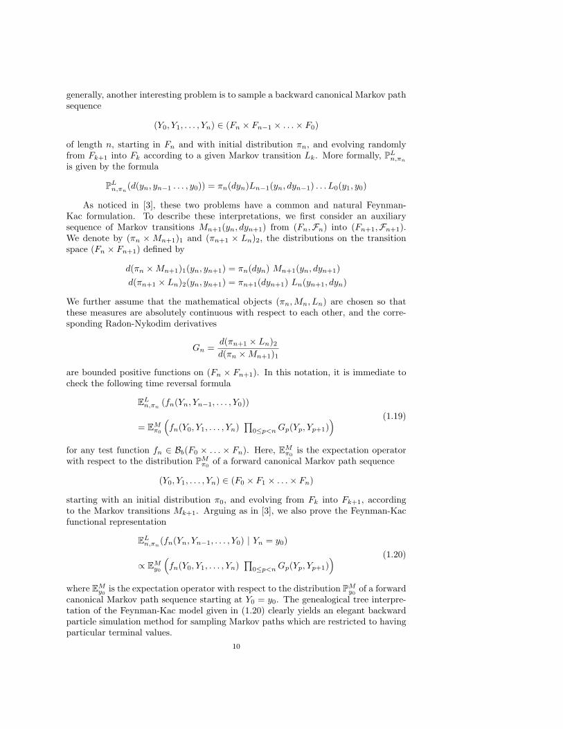
generally, another interesting problem is to sample a backward canonical Markov pathsequence

(Y0, Y1, . . . , Yn) ∈ (Fn × Fn−1 × . . .× F0)

of length n, starting in Fn and with initial distribution πn, and evolving randomlyfrom Fk+1 into Fk according to a given Markov transition Lk. More formally, PL

n,πn

is given by the formula

PLn,πn

(d(yn, yn−1 . . . , y0)) = πn(dyn)Ln−1(yn, dyn−1) . . . L0(y1, y0)

As noticed in [3], these two problems have a common and natural Feynman-Kac formulation. To describe these interpretations, we first consider an auxiliarysequence of Markov transitions Mn+1(yn, dyn+1) from (Fn,Fn) into (Fn+1,Fn+1).We denote by (πn × Mn+1)1 and (πn+1 × Ln)2, the distributions on the transitionspace (Fn × Fn+1) defined by

d(πn ×Mn+1)1(yn, yn+1) = πn(dyn) Mn+1(yn, dyn+1)d(πn+1 × Ln)2(yn, yn+1) = πn+1(dyn+1) Ln(yn+1, dyn)

We further assume that the mathematical objects (πn,Mn, Ln) are chosen so thatthese measures are absolutely continuous with respect to each other, and the corre-sponding Radon-Nykodim derivatives

Gn =d(πn+1 × Ln)2d(πn ×Mn+1)1

are bounded positive functions on (Fn × Fn+1). In this notation, it is immediate tocheck the following time reversal formula

ELn,πn

(fn(Yn, Yn−1, . . . , Y0))

= EMπ0

(fn(Y0, Y1, . . . , Yn)

∏0≤p<n Gp(Yp, Yp+1)

) (1.19)

for any test function fn ∈ Bb(F0 × . . . × Fn). Here, EMπ0

is the expectation operatorwith respect to the distribution PM

π0of a forward canonical Markov path sequence

(Y0, Y1, . . . , Yn) ∈ (F0 × F1 × . . .× Fn)

starting with an initial distribution π0, and evolving from Fk into Fk+1, accordingto the Markov transitions Mk+1. Arguing as in [3], we also prove the Feynman-Kacfunctional representation

ELn,πn

(fn(Yn, Yn−1, . . . , Y0) | Yn = y0)

∝ EMy0

(fn(Y0, Y1, . . . , Yn)

∏0≤p<n Gp(Yp, Yp+1)

) (1.20)

where EMy0

is the expectation operator with respect to the distribution PMy0

of a forwardcanonical Markov path sequence starting at Y0 = y0. The genealogical tree interpre-tation of the Feynman-Kac model given in (1.20) clearly yields an elegant backwardparticle simulation method for sampling Markov paths which are restricted to havingparticular terminal values.

10

These particle approximation models can also be interpreted as a sequence ofinteracting Metropolis type algorithms. We illustrate this observation in the contextof the target Boltzmann-Gibbs measures introduced in (1.18). In this case, we no-tice that, the n-th marginal of the Feynman-Kac path measure introduced in (1.19)coincides with the Boltzmann-Gibbs measure at temperature βn; that is, we have

EMπ0

ϕn(Yn)∏

0≤p<n

Gp(Yp, Yp+1)

= πn(ϕn) (1.21)

for any ϕn ∈ Bb(En). In contrast to traditional non-interacting Metropolis models,we emphasize that the McKean interpretation (1.5) of the flow (1.21) consists of anonlinear Markov chain with distribution πn, at each time n. Furthermore, the corre-sponding particle interpretation clearly behaves as an interacting Metropolis model.It is also essential to notice that the usual Metropolis rejection mechanism has beenreplaced by a selective interacting jump transition. As noticed in [4]; in practice, onejudicious choice of Markov mutation transition is to take a Markov chain Monte Carlokernel Mn such that πnMn = πn. In this case, the interaction potential functions aregiven by

Gn(yn, yn+1) = exp [−(βn+1 − βn)V (yn)]

as soon as Ln(yn+1, dyn) = πn+1(dyn) dMn+1(yn,.)dπn+1

(yn+1). When Mn represents theelementary transition of a simulated annealing model at temperature βn, the result-ing particle model behaves as an interacting simulated annealing algorithm. At lowtemperature, the potential function is close to one, and thus the particles are morelikely not to interact.

1.3.2. Nonlinear filtering problems. The filtering problem is to estimate astochastic signal process that we cannot observe directly. More precisely, the signalis partially observed by some noisy sensors. The noise may come from the modeluncertainties, or from inherent perturbations, such as thermal noise in electronicdevices.

The signal/observation pair sequence (Xn, Yn)n≥0 is defined as a Markov chainwhich takes values in some product of measurable spaces (En × Fn)n≥0. We furtherassume that the initial distribution ν0 and the Markov transitions Pn of (Xn, Yn) havethe form

ν0(d(x0, y0)) = g0(x0, y0) η0(dx0) q0(dy0)Pn((xn−1, yn−1), d(xn, yn)) = gn(xn, yn) Mn(xn−1, dxn) qn(dyn)

where gn are strictly positive functions on (En×Fn) and qn is a sequence of measureson Fn. The initial distribution η0 of the signal Xn, and its Markov transitions Mn

from En−1 into En, are assumed known. A version of the conditional distributions ofthe signal states given their noisy observations is expressed in terms of Feynman-Kacformulae of the same type as the ones discussed. More precisely, let Gn be the nonhomogeneous function on En defined for any xn ∈ En by

Gn(xn) = gn(xn, yn). (1.22)

Note that Gn depends on the observation value yn at time n. In this notation, theconditional distribution of the signal Xn, given the sequence of observations from the

11

origin up to time n, has the Feynman-Kac functional representation

E(fn(X0, . . . , Xn) | Y0 = y0, . . . , Yn = yn) ∝ E(fn(X0, . . . , Xn)∏

0≤p≤n Gp(Xp)).

In this context, the corresponding genealogical tree based models can be interpretedas an adaptive and stochastic grid approximation. Note that the selection transitionis dictated by the likelihood function (1.22); i.e. the current observation deliveredby the sensors. Therefore, the resulting birth and death genetic mechanism givesmore reproductive opportunities to particles evolving in state space regions with highconditional probability mass. This filtering problem arises in numerous scientific dis-ciplines, including financial mathematics, robotics, telecommunications and tracking;see for instance [2, 7], and references therein.

2. Preliminary results. This section is decomposed into two separate parts.In the first subsection, Subsection 2.1, we provide a summary of results on the fluc-tuations of a class of random fields associated with the particle occupation measuresηN

n introduced in (1.6). The definitions and results come essentially from Chapter9 in the monograph [2]. We shall simplify and further extend this study to randomfield product models. This approach is central in our method of analyzing the sharpasymptotic propagation of chaos properties. In Subsection 2.2, we provide a trans-port equation relating a pair of q-tensor product particle measures. We also mentionthat weaker versions of this identity are sometimes used in nonparametric statisticsto relate U -statistics to von Mises statistics.

2.1. Fluctuation analysis. The fluctuation analysis of the particle measuresηN

n around their limiting values ηn is essentially based on the asymptotic analysis ofthe local sampling errors associated with the particle approximation sampling steps.These local errors are expressed in terms of the random fields WN

n , given for anyfn ∈ Bb(En) by the formula

WNn (fn) =

√N [ηN

n −Ψn−1(ηNn−1)Mn](fn) =

1√N

N∑i=1

[fn(ξin)−Kn,ηN

n−1(fn)(ξi

n−1)].

The next central limit theorem for random fields is pivotal. Its complete proofcan be found in [2] (theorem 9.3.1, and corollary 9.3.1, pp. 295-298).

Theorem 2.1. For any fixed time horizon n ≥ 1, the sequence (WNp )1≤p≤n

converges in law, as N tends to infinity, to a sequence of n independent, Gaussianand centered random fields (Wp)1≤p≤n; with, for any fp, gp ∈ Bb(Ep), and 1 ≤ p ≤ n,

E(Wp(fp)Wp(gp)) = ηp−1Kp,ηp−1([fp −Kp,ηp−1(fp)][gp −Kp,ηp−1(gp)]) (2.1)

For the McKean selection transition (1.4), with εn = 0, we find that

Kp,ηp−1(xp−1, .) = Ψp−1(ηp−1)Mp.

In this case, the correlation term (2.1) takes the form

E(Wp(fp)Wp(gp)) = ηp([fp − ηp(fp)][gp − ηp(gp)]).12

More generally, for any choice of εn ≥ 0, we have

E(Wp(fp)Wp(gp)) = ηp([fp − ηp(fp)][gp − ηp(gp)])

− ηp−1((εp−1Gp−1)2[Mp(fp)− ηp(fp)][Mp(gp)− ηp(gp)])= ηp([fp − ηp(fp)][gp − ηp(gp)])

− ε2p−1ηp−1(Qp−1,p[fp − ηp(fp)]Qp−1,p[gp − ηp(gp)]).

These two observations show that local variances induced by sampling errors arereduced for the McKean transitions associated with the choice εn > 0.

These multivariate fluctuations also yield, for any finite collection of functions(f (i)

n )1≤i≤d ∈ Bb(En)d, with d ≥ 1

(WNn (f1

n), . . . ,WNn (fd

n)) −→N→∞ (Wn(f1p1

), . . . ,Wn(fdn))

where (Wn(f1n), . . . ,Wn(fd

n)) is a d-dimensional centered Gaussian random variablewith a (d× d)-covariance matrix Σ(f) whose (i, j)-elements Σ(f i

n, f jn) are given by

Σ(f in, f j

n) = ηn−1Kn,ηn−1([fin −Kn,ηn−1(f

in)][f j

n −Kn,ηn−1(fjn)]).

We also observe that the unnormalized distributions (γn) can be expressed interms of the normalized measures with the product formula γn+1(1) = γn(Gn) =ηn(Gn) γn(1). This readily implies that, for any fn ∈ Bb(Fn),

γn(fn) = ηn(fn)∏

0≤p<n

ηp(Gp). (2.2)

Mimicking (2.2), the unbiased particle approximation measures γNn of the unnor-

malized model γn are defined as

γNn (fn) = ηN

n (fn)∏

0≤p<n

ηNp (Gp).

To explain what we have in mind when making these definitions, we now consider theelementary decomposition

γNn − γn =

n∑p=0

[γNp Qp,n − γN

p−1Qp−1,n]

For p = 0, we take the convention ηN−1Q−1,n = γn. The next important thing to note

is that

γNp−1Qp−1,p = γN

p−1(Gp−1)Ψp−1(ηNp−1)Mp and γN

p−1(Gp−1) = γNp (1)

This decomposition now readily implies that

W γ,Nn (fn) =def.

√N [γN

n − γn](fn) =n∑

p=0

γNp (1) WN

p (Qp,nfn) (2.3)

Since the random variable γNp (1) only depends on the flow (ηN

k )0≤k<p, it is easy tocheck that γN

n is an unbiased estimate of γn; in the sense that E(γNn (fn)) = γn(fn),

for any fn ∈ Bb(En). To take the final step, we recall that the random sequence13

(γNp (1))1≤p≤n converges in law, as N tends to infinity, to the deterministic sequence

(γp(1))1≤p≤n (see, for instance, [2]). A simple application of Slutsky’s Lemma, impliesthat the random fields W γ,N

n converge in law, as N tends to infinity, to the Gaussianrandom fields W γ

n defined for any fn ∈ Bb(En) by

W γn (fn) =

n∑p=0

γp(1) Wp(Qp,nfn) (2.4)

In much the same way, the sequence of random fields

W η,Nn (fn) =def.

√N [ηN

n − ηn](fn)

= γNn (1)

−1 × W γ,Nn (fn − ηn(fn)) (2.5)

converge in law, as N tends to infinity, to the Gaussian random fields W ηn defined for

any fn ∈ Bb(En) by

W ηn (fn) =

n∑p=1

(γp(1)/γn(1)) Wp (Qp,n(fn − ηn(fn))) (2.6)

Our final objective is to analyze the asymptotic behavior of random fields ofproduct sequences. These properties are one of the stepping stones in the integrationanalysis of propagation of chaos used in the further development of Section 3.

We let Poly(Eqn) be the set of all linear combinations Fn =

∑k≥0 λk F k

n ofpolynomial q-tensor product functions

F kn = f (k,1)

n ⊗ . . .⊗ f (k,q)n , with (f (k,i)

n )1≤i≤q ∈ Bb(En)q

where∑

k≥0 |λk| ‖F kn‖ < ∞. We are now ready to prove the following proposition.

Proposition 2.2. For any time horizon n ≥ 1, any particle block size parameter1 ≤ q ≤ N and any sequence (νi)1≤i≤d ∈ {γ, η}, the sequence of random fields(W ν1,N

n ⊗ . . .⊗W νq,Nn ) on Poly(Eq

n) converges in law, as N tends to infinity, to theGaussian random field (W ν1

n ⊗. . .⊗W νq

n ). In addition, we have for any Fn ∈ Poly(Eqn)

limN→∞

E((W ν1,N

n ⊗ . . .⊗W νq,Nn )(Fn)

)= E

((W ν1

n ⊗ . . .⊗W νq

n )(Fn))

Proof:We recall from [2] that for ν ∈ {γ, η}, for any fn ∈ Bb(En), and p ≥ 1, we have theLp-mean error estimates

supN≥1

E(|W ν,Nn (fn)|p)1/p ≤ cp(n) ‖fn‖ (2.7)

for some finite constant cp(n), which depends only on the pair of parameters (p, n), andwith the random fields (W γ,N

n ,W η,Nn ) defined in (2.3) and (2.5). By the Borel-Cantelli

lemma this property ensures that the random sequence of pairs (γNn (fn), ηN

n (fn))converges almost surely to (γn(fn), ηn(fn)), as N tends to infinity. By the definitionsof the random fields (W γ,N

n ,W η,Nn ) given in (2.3) and (2.5), and recalling that the

sequence of random fields (WNp )1≤p≤n converges in law, as N tends to infinity, to

a sequence of n independent, Gaussian and centered random fields (Wp)1≤p≤n, oneconcludes that

(W ν1,Nn ⊗ . . .⊗W νq,N

n )(f (k,1)n ⊗ . . .⊗ f (k,q)

n ) =q∏

i=1

W νi,Nn (f (k,i)

n )

14

converges in law, as N tends to infinity, to

(W ν1

n ⊗ . . .⊗W νq

n )(f (k,1)n ⊗ . . .⊗ f (k,q)

n ) =q∏

i=1

W νi

n (f (k,i)n ).

for any (f (k,i)n )1≤i≤q ∈ Bb(En)q. This clearly ends the proof of the first assertion.

Using Holder’s inequality, we can also prove that any polynomial function of afinite number of terms W ν,N

n (fn), with ν ∈ {γ, η} and fn ∈ Bb(En), forms a uniformlyintegrable collection of random variables (indexed by the size and precision param-eter N ≥ 1). This property, combined with the continuous mapping theorem, andSkorohod embedding theorem, end the proof of the proposition.

2.2. Combinatorial properties of tensor product measures. This sectionis concerned with a precise combinatorial analysis of the particle measures on Eq

n

defined by the formulae

(ηNn )⊗q =

1Nq

∑β∈〈N〉〈q〉

δ(ξ

β(1)n ,..., ξ

β(q)n )

and (ηNn )�q =

1(N)q

∑β∈<q,N>

δ(ξ

β(1)n ,..., ξ

β(q)n )

(2.8)

where 〈N〉〈q〉 represents the set of all mappings from 〈q〉 = {1, . . . , q} into 〈N〉, and〈q, N〉 the subset of all (N)q = N !/(N − q)! one-to-one mappings from the set 〈q〉into 〈N〉. More precisely, the aim of this short section is to express (ηN

n )⊗q as a lineartransport of the measure (ηN

n )�q, with respect to some Markov transition. As weshall see in the further development of section 3 , this property allows direct transferof several asymptotic results on the q-tensor product measures (ηN

n )⊗q to the randommeasures (ηN

n )�q.We let P(q, p) be the set of all partitions of the set 〈q〉 into p blocks, equipped

with the order relation on the subsets A,B of 〈q〉 given by

A ≤ B ⇐⇒ inf {i : i ∈ A} ≤ inf {i : i ∈ B}.

Finally, we associate with a given partition π = (πi)1≤i≤p ∈ P(q, p), of p increasingblocks, the mapping βπ ∈< q, N > defined by βπ =

∑pi=1 β(i) 1πi . In this notation,

we have for any Fn ∈ Bb(Eqn)

(ηNn )�q(Fn) =

1(N)q

∑β∈<q,N>

(Fn)(ξβ(1)n , . . . , ξβ(q)

n ) (2.9)

and

(ηNn )⊗q(Fn) =

1Nq

q∑p=1

∑π∈P(q,p)

∑β∈<p,N>

Fn(ξβπ(1)n , . . . , ξβπ(q)

n ) (2.10)

The latter formula is reasonably well known (for a complete proof we refer the readerto [2], section 8.6, on page 267). For symmetric test functions Fn, if we replace therandom sequence (ξi

n)1≤i≤N by a sequence of independent and identically distributedrandom variables, then these two quantities are known as the U -statistics, and theV -statistics or the von Mises statistics of degree q with kernel Fn. These two objects

15

appear in a natural way in generalized mean valued statistics analysis. The simplestnontrivial example often used is the 2-tensor product measure. In this case, we have

P(2, 1) = {π} with π = {π1, π2} and π1 = {1} ≤ π2 = {2}P(2, 2) = {π} with π = π1 = {1, 2}

Thus, equations (2.9) and (2.10) for q = 2, takes the simplest form

(ηNn )�2(Fn) =

1N(N − 1)

∑β∈<2,N>

Fn(ξβ(1)n , ξβ(2)

n )

and

(ηNn )⊗2(Fn) =

1N2

∑β∈<1,N>

Fn(ξβ(1)n , ξβ(1)

n ) +1

N2

∑β∈<2,N>

Fn(ξβ(1)n , ξβ(2)

n ).

In a more general set-up, we observe that the q-th term in the r.h.s. of (2.10) is givenby

1Nq

∑β∈<q,N>

Fn(ξβ(1)n , . . . , ξβ(q)

n )

For p = (q−1), the set P(q, q−1) consists of all q(q−1)/2 partitions π with one block oftwo elements, and (q−2) blocks of one element. For instance, for π = {π1, . . . , πq−1},with

π1 = {1, 2} ≤ π2 = {3} ≤ . . . ≤ πq−1 = {q}

we find that∑β∈<q−1,N>

Fn(ξβπ(1)n , . . . , ξβπ(q)

n ) =∑

β∈<q−1,N>

Fn(ξβ(1)n , ξβ(1)

n , ξβ(2)n . . . , ξβ(q−1)

n ).

To go one step further in our discussion, we observe that, for any p ≤ q, we have

Fn(ξβπ(1)n , . . . , ξβπ(q)

n ) = Cp,qπ (Fn)(ξβ(1)

n , . . . , ξβ(p)n ),

with the Markov operator Cp,qπ from Ep

n into Eqn defined by

Cp,qπ (Fn)(x1, . . . , xp) = Fn(

p∑i=1

xi 1πi(1), . . . ,

p∑i=1

xi 1πi(q)).

We extend Cp,qπ to a Markov operator C

(p,q)π from Eq

n into itself by setting

C(p,q)π (Fn)(x1, . . . , xq) = Cp,q

π (Fn)(x1, . . . , xp).

The operator C(p,q)π has the following interpretation; let π be a partition of q elements

into p increasing blocks π1, . . . , πp of respective sizes b1, . . . , bp. Sampling a configu-ration according to C

(p,q)π ((x1, . . . , xq), .) consists of duplicating the individuals xi, bi

times, where 1 ≤ i ≤ p. In this sense, C(p,q)π can also be interpreted as a selection16

jump operator. By construction, an elementary calculation provides the followingidentities

1(N)p

∑β∈<p,N>

Fn(ξβπ(1)n , . . . , ξβπ(q)

n ) = (ηNn )�pCp,q

π Fn = (ηNn )�qC(p,q)

π Fn.

Using (2.10), it is straightforward to prove the following Markov transport equation.Proposition 2.3. For any block size parameter 1 ≤ q ≤ N , we have the decom-

position

(ηNn )⊗q =

1Nq

q∑p=1

S(q, p) (N)p (ηNn )�qC(p,q), (2.11)

with S(q, p) is the Stirling number of the second kind∗, and the Markov selection-jumptype operator C(p,q) from Eq

n into itself is given by

C(p,q) =1

S(q, p)

∑π∈P(q,p)

C(p,q)π .

In our context, the special attractiveness of the decomposition (2.11) comes from thefact that it connects in a natural way the distribution P(q,N)

n of the first q particles(ξ1

n, . . . , ξqn) with the mean value of the q-tensor product measures (ηN

n )⊗q. Moreprecisely, by the exchangeability property of the particle model, we have the followingtransport equation

E[(ηNn )⊗q(Fn)] =

1Nq

q∑p=1

S(q, p) (N)p P(q,N)n (C(p,q)(Fn)) = P(q,N)

n C(q,N)(Fn)

for any Fn ∈ Bb(Eqn), with the Markov transition from Eq

n into itself given by

C(q,N) =def.

1Nq

q∑p=1

S(q, p) (N)p C(p,q)

3. Asymptotic propagation of chaos properties. The main objective of thissection is to prove the theorems stated in Section 1.2.

In Subsection 3.1 we provide a weak asymptotic expansion of the distributionP(q,N)

n of the first q particles (ξin)1≤i≤q on tensor product functions. We analyze a

general class of McKean selection models (1.4). The study is decomposed into twoparts. First we examine the bias of the tensor product particle measures (ηN

n )⊗q usingthe random field fluctuation analysis presented in Subsection 2.1. Then we transferthis result to P(q,N)

n with the help of the combinatorial transport equation developedin Subsection 2.2.

In Subsection 3.3, we extend the weak asymptotic expansions derived in Subsec-tion 3.1 to the class of continuous and bounded functions on product spaces. Thisanalysis is restricted to a simple genetic particle model evolving on locally compactand separable metric spaces. We recall that these genetic models correspond to theMcKean selection transition (1.4), with εn = 0. Our strategy consists of analyzingthe tensor product bias, and the asymptotic first order quantities as linear functionaloperators. This integration of a propagation of chaos interpretation, combined witha density argument allows us to derive an asymptotic expansion P(q,N)

n .

∗S(q, p) corresponds to the number of partitions of q elements in p blocks.

17

3.1. General McKean particle models. As we mentioned above, Proposi-tion 2.2 is pivotal in the analysis of the bias of the path-particle models. To illustrateour approach, we present an elementary consequence of Proposition 2.2. We firstrewrite (2.5) as follows

W η,Nn (fn)

= γn(1)−1W γ,N

n (fn − ηn(fn)) +(γN

n (1)−1 − γn(1)−1)× Wγ,N

n ((fn − ηn(fn)))

= γn(1)−1W γ,N

n (fn − ηn(fn))− 1√N

[γNn (1)γn(1)]−1 W γ,N

n (fn − ηn(fn))W γ,Nn (1).

This readily yields that

N E(ηNn (fn)− ηn(fn)) = −E

([γN

n (1)γn(1)]−1 W γ,Nn (fn − ηn(fn))W γ,N

n (1)).

Note that the random sequence (1/(γn(1)γNn (1)))N≥1 is uniformly bounded, and it

converges in law to γn(1)−2, as N tends to infinity. Now using Proposition 2.2, wefind the sharp asymptotic bias estimate

limN→∞ N E(ηNn (fn)− ηn(fn))

= −γn(1)−2 E (W γn (1) W γ

n (fn − ηn(fn)))

= −n∑

p=0

(γp(1)/γn(1))2 E (Wp(Qp,n(1)) Wp(Qp,n[fn − ηn(fn)])) . (3.1)

The next technical proposition extends this result to the tensor empirical measures(ηN

n )⊗q.Proposition 3.1. For any n, q ≥ 1, and every sequence of functions f

(k)n ∈

Bb(En), with ηn(f (k)n ) = 1, and 1 ≤ k ≤ q, we have

limN→∞ N E[∏q

k=1 ηNn (f (k)

n )− 1]

= −q∑

i=1

γn(1)−2 E(W γ

n (1) W γn

(f (i)

n − 1))

+∑

1≤i<j≤q

E(W η

n (f (i)n )W η

n (f (j)n ))

.

Proof:We use the decomposition

q∏i=1

ai − 1 =∑

1≤p≤q

∑1≤j1<...<jp≤q

p∏l=1

(ajl− 1)

which is valid for any q ≥ 0, and any collection of real numbers (ai)1≤i≤q. Using (2.7)and Holder’s inequality we readily find that

|E[q∏

p=1

(ηNn (f (p)

n )− 1)]| ≤q∏

p=1

E[|ηNn (f (p)

n )− 1|q]1/q ≤ cq(n)Nq/2

[q∏

p=1

‖f (p)n ‖]

18

for some finite constant cq(n), which depends only on the pair of parameters (q, n).If we take ai = ηN

n (f (i)n ) in the above decomposition, then we obtain

q∏p=1

ηNn (f (p)

n )− 1 =∑

1≤p≤q

∑1≤j1<...<jp≤q

N−p/2

[p∏

l=1

W η,Nn (f (jl)

n )

](3.2)

from which we conclude that

E[∏q

k=1 ηNn (f (k)

n )− 1]

=∑q

i=1 E[(ηN

n (f (i)n )− 1

]+∑

1≤i<j≤q E[(ηN

n (f (i)n )− 1)(ηN

n (f (j)n )− 1)

]+ O

(1

N√

N

).

The end of the proof is now a straightforward consequence of (3.1) and Proposition 2.2.

The statement of Proposition 3.1 corresponds to the first part of the Theorem 1.1.Indeed, by the definitions of the random fields (W γ

n ,W ηn ) given in (2.4) and (2.6), and

for every sequence of functions f(k)n ∈ Bb(En), with ηn(f (i)

n ) = 1, and 1 ≤ i ≤ q, wehave that

E(W γ

n (1) W γn

(f (i)

n − 1))

=n∑

p=0

n∑q=0

γp(1) γq(1) E[Wp(Qp,n(1)) Wq(Qq,n(f (i)

n − 1))]

=n−1∑p=0

γp(1)2 E[Wp(Qp,n(1)) Wp(Qp,n(f (i)

n − 1))]

and

E(W η

n

(f

(i)n

)W η

n

(f

(j)n

))=∑n

p=0

(γp(1)γn(1)

)2

E[Wp(Qp,n(f (i)

n − 1)) Wp(Qp,n(f (j)n − 1)

]=∑n

p=0 E[Wp(Rp,n(f (i)

n − 1)) Wp(Rp,n(f (j)n − 1)

]This implies that

limN→∞

N E

[q∏

k=1

ηNn (f (k)

n )− 1

]

= −∑q

i=1

∑n−1p=0 γp(1)2 E

(Wp(Qp,n1) Wp(Qp,n[f (i)

n − 1]))

+∑

1≤i<j≤q

∑np=0 E

(Wp(Rp,n(f (i)

n − 1))Wp(Rp,n(f (j)n − 1))

)

19

The end of the proof of the theorem is now a clear consequence of the followingproposition.

Proposition 3.2. For any time horizon n ≥ 1, any particle block size parameter1 ≤ q ≤ N , and every sequence of functions f

(k)n ∈ Bb(En), with ηn(f (k)

n ) = 1, and1 ≤ k ≤ q, we have

limN→∞ N[E(f

(1)n (ξ1

n) . . . f(q)n (ξq

n))− 1]

= −∑q

i=1 γn(1)−2 E(W γ

n (1) W γn

(f

(i)n − 1

))+∑

1≤i<j≤q

[E(W η

n (f (i)n )W η

n (f (j)n ))

+(1− ηn(f (i)

n f(j)n ))]

Proof:After some elementary manipulations, and using (2.11), we prove that

E((ηN

n )⊗q(f (1)n ⊗ . . .⊗ f (q)

n ))− 1 =

(N)q

NqI(1,N)n (f) +

(N)q−1

NqI(2,N)n (f) + O

(1

N2

)(3.3)

with

I(1,N)n (f) = E

((ηN

n )�q(f (1)n ⊗ . . .⊗ f (q)

n ))− 1 = E(f (1)

n (ξ1n) . . . f (q)

n (ξqn))− 1

and

I(2,N)n (f) =

∑π∈P(q,q−1)

E((ηN

n )�(q−1)Cq−1,qπ

((f (1)

n ⊗ . . .⊗ f (q)n )− 1

))

=∑

1≤i<j≤q

E

(f (i)n f (j)

n )(ξin) [

∏k∈{1,...,q}−{i,j}

f (k)n (ξk

n)]

− 1

.

Meanwhile, by (1.9) we observe that limN→∞ I(1,N)n (f) = 0, and since we have

N

[1− (N)q

Nq

]≤ N

[1−

(1− q − 1

N

)q−1)≤ (q − 1)2

we also find that limN→∞ N(1− (N)q

Nq

)I(1,N)n (f) = 0. In much the same way, we

have

limN→∞

I(2,N)n (f) = I(2)

n (f) =def.

∑1≤i<j≤q

[ηn(f (i)

n f (j)n )− 1

].

This clearly yields that limN→∞ (N)q−1N−(q−1) I

(2,N)n (f) = I

(2)n (f). These estimates

together with (3.3) imply that

limN→∞

N I(1,N)n (f) = −I(2)

n (f) + limN→∞

N E

[q∏

k=1

ηNn (f (k)

n )− 1

].

The end of the proof is now a straightforward consequence of Proposition 3.1.

20

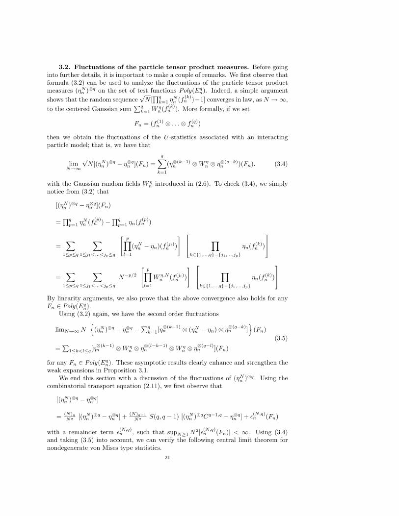
3.2. Fluctuations of the particle tensor product measures. Before goinginto further details, it is important to make a couple of remarks. We first observe thatformula (3.2) can be used to analyze the fluctuations of the particle tensor productmeasures (ηN

n )⊗q on the set of test functions Poly(Eqn). Indeed, a simple argument

shows that the random sequence√

N [∏q

k=1 ηNn (f (k)

n )−1] converges in law, as N →∞,to the centered Gaussian sum

∑qk=1 W η

n (f (k)n ). More formally, if we set

Fn = (f (1)n ⊗ . . .⊗ f (q)

n )

then we obtain the fluctuations of the U -statistics associated with an interactingparticle model; that is, we have that

limN→∞

√N [(ηN

n )⊗q − η⊗qn ](Fn) =

q∑k=1

(η⊗(k−1)n ⊗W η

n ⊗ η⊗(q−k)n )(Fn). (3.4)

with the Gaussian random fields W ηn introduced in (2.6). To check (3.4), we simply

notice from (3.2) that

[(ηNn )⊗q − η⊗q

n ](Fn)

=∏q

p=1 ηNn (f (p)

n )−∏q

p=1 ηn(f (p)n )

=∑

1≤p≤q

∑1≤j1<...<jp≤q

[p∏

l=1

(ηNn − ηn)(f (jl)

n )

] ∏k∈{1,...,q}−{j1,...,jp}

ηn(f (k)n )

=∑

1≤p≤q

∑1≤j1<...<jp≤q

N−p/2

[p∏

l=1

W η,Nn (f (jl)

n )

] ∏k∈{1,...,q}−{j1,...,jp}

ηn(f (k)n )

By linearity arguments, we also prove that the above convergence also holds for anyFn ∈ Poly(Eq

n).Using (3.2) again, we have the second order fluctuations

limN→∞ N{

(ηNn )⊗q − η⊗q

n −∑q

k=1[η⊗(k−1)n ⊗ (ηN

n − ηn)⊗ η⊗(q−k)n ]

}(Fn)

=∑

1≤k<l≤q[η⊗(k−1)n ⊗W η

n ⊗ η⊗(l−k−1)n ⊗W η

n ⊗ η⊗(q−l)n ](Fn)

(3.5)

for any Fn ∈ Poly(Eqn). These asymptotic results clearly enhance and strengthen the

weak expansions in Proposition 3.1.We end this section with a discussion of the fluctuations of (ηN

n )�q. Using thecombinatorial transport equation (2.11), we first observe that

[(ηNn )⊗q − η⊗q

n ]

= (N)q

Nq [(ηNn )�q − η⊗q

n ] + (N)q−1Nq S(q, q − 1) [(ηN

n )�qCq−1,q − η⊗qn ] + ε

(N,q)n (Fn)

with a remainder term ε(N,q)n , such that supN≥1 N2|ε(N,q)

n (Fn)| < ∞. Using (3.4)and taking (3.5) into account, we can verify the following central limit theorem fornondegenerate von Mises type statistics.

21

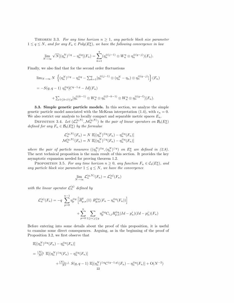
Theorem 3.3. For any time horizon n ≥ 1, any particle block size parameter1 ≤ q ≤ N , and for any Fn ∈ Poly(Eq

n), we have the following convergence in law

limN→∞

√N [(ηN

n )�q − η⊗qn ](Fn) =

q∑k=1

(η⊗(j−1)n ⊗W η

n ⊗ η⊗(q−j)n )(Fn).

Finally, we also find that for the second order fluctuations

limN→∞ N{

(ηNn )�q − η⊗q

n −∑q

k=1[η⊗(j−1)n ⊗ (ηN

n − ηn)⊗ η⊗(q−j)n ]

}(Fn)

= −S(q, q − 1) η⊗qn [Cq−1,q − Id](Fn)

+∑

1≤k<l≤q[η⊗(k−1)n ⊗W η

n ⊗ η⊗(l−k−1)n ⊗W η

n ⊗ η⊗(q−l)n ](Fn).

3.3. Simple genetic particle models. In this section, we analyze the simplegenetic particle model associated with the McKean interpretation (1.4), with εn = 0.We also restrict our analysis to locally compact and separable metric spaces En.

Definition 3.4. Let (L(q,N)n ,M(q,N)

n ) be the pair of linear operators on Bb(Eqn)

defined for any Fn ∈ Bb(Eqn) by the formulae

L(q,N)n (Fn) = N E[(ηN

n )⊗q(Fn)− η⊗qn (Fn)]

M(q,N)n (Fn) = N E[(ηN

n )�q(Fn)− η⊗qn (Fn)]

where the pair of particle measures ((ηNn )⊗q, (ηN

n )�q) on Eqn are defined in (2.8).

The next technical proposition is the main result of this section. It provides the keyasymptotic expansion needed for proving theorem 1.2.

Proposition 3.5. For any time horizon n ≥ 0, any function Fn ∈ Cb(Eqn), and

any particle block size parameter 1 ≤ q ≤ N , we have the convergence

limN→∞

L(q,N)n (Fn) = L(q)

n (Fn)

with the linear operator L(q)n defined by

L(q)n (Fn) = −q

n−1∑p=0

η⊗qp

[R

q

p,n(1) R⊗qp,n(Fn − η⊗q

n (Fn))]

+n∑

p=0

∑1≤i<j≤q

η⊗qp Ci,jR

⊗qp,n(Id− pi

n)(Id− pjn)(Fn)

Before entering into some details about the proof of this proposition, it is usefulto examine some direct consequences. Arguing, as in the beginning of the proof ofProposition 3.2, we first observe that

E[(ηNn )⊗q(Fn)− η⊗q

n (Fn)]

= (N)q

Nq E[(ηNn )�q(Fn)− η⊗q

n (Fn)]

+ (N)q−1Nq S(q, q − 1) E[(ηN

n )�qC(q−1,q)(Fn)− η⊗qn (Fn)] + O(N−2)

22

The propagation of chaos estimate presented in (1.9), combined with the exchange-ability property of the particle configurations, implies that

N |E((ηNn )�qC(p,q)(Fn))− η⊗q

n C(p,q)(Fn)| ≤ q2 c(n) ‖Fn‖

for any 1 ≤ p ≤ q ≤ N , and any function Fn ∈ Bb(Eqn). From these estimates we also

deduce that

L(q)n (Fn) = M(q)

n (Fn) +q(q − 1)

2η⊗q

n [C(q−1,q) − Id](Fn)

where the bounded linear operator M(q)n on Bb(Eq

n) is given by

M(q)n (Fn) =def. lim

N→∞N E[(ηN

n )�q(Fn)− η⊗qn (Fn)]

As an aside, using (1.9) again, we find that |M(q)n (Fn)| ≤ c(n) q2 ‖Fn‖. In conclusion,

for any Fn ∈ Cb(Eqn), n ≥ 1, and 1 ≤ q ≤ N we have proved that

limN→∞

N E[Fn(ξ1n, . . . , ξq

n)− η⊗qn (Fn)] = M(q)

n (Fn)

where the bounded linear operator Mn on Cb(Eqn) is given by

M(q)n (Fn) = L(q)

n (Fn)−∑

1≤i<j≤q

η⊗qn [Ci,j − Id](Fn)

where L(q)n is the operator defined in (3.7). This clearly ends the proof of theorem 1.2.

We are now in a position to prove the announced proposition.Proof of proposition 3.5 :By (2.11), we have that

L(q,N)n (Fn)

=(N)q

NqM(q,N)

n (Fn) +1

Nq−1

q−1∑p=1

S(q, p) (N)p E[(C(p,q) − Id)Fn(ξ1

n, . . . , ξqn)].

By the propagation of chaos estimates presented in (1.9), we have the bounds

supN≥1

sup‖Fn‖≤1

{|L(q,N)n (Fn)| ∨ |M(q,N)

n (Fn)|} ≤ c(n) (q2 +q−1∑p=1

S(q, p)). (3.6)

In other words, (L(q,N)n )N≥1, and (M(q,N)

n )N≥1 are uniformly bounded sequences oflinear operators on Bb(Eq

n). On the other hand, for polynomial functions of the form

Fn = f (1)n ⊗ . . .⊗ f (q)

n

with (f (k)n )1≤k≤q ∈ Bb(Eq), we have, from Proposition 3.1,

limN→∞

N E[(ηNn )⊗q(Fn)− η⊗q

n (Fn)] = L(q)n (Fn) =def. L(q),1

n (Fn) + L(q),2n (Fn)

(3.7)

23

where the pair of linear operators (L(q),1n ,L(q),2

n ) are defined by

L(q),1n (Fn) = −

q∑i=1

γn(1)−2 E[W γ

n (1) W γn

(f (i)

n − ηn(f (i)n ))]

[∏

1≤j≤q, j 6=i

ηn(f (j)n )],

L(q),2n (Fn) =

∑1≤i<j≤q

E(W η

n (f (i)n )W η

n (f (j)n ))

[∏

1≤k≤q, k 6∈{i,j}

ηn(f (k)n )].

By the definition of the random field W ηn given in (2.4), we find that

γn(1)−2 E[W γ

n (1) W γn

(f

(i)n − ηn(f (i)

n ))]

=∑n

p=0 ηp[Rp,n(1) Rp,n(f (i)n − ηn(f (i)

n ))]

=∑n

p=0 ηp[Rp,n(1) Rp,n(f (i)n )]− ηn(f (i)

n )∑n

p=0 ηp[Rp,n(1)2].

¿From these observations, we obtain the operator decomposition

L(q),1n (Fn) =

n∑p=0

L(q),1p,n (Fn)

with the collection of linear operators L(q),1p,n given by

L(q),1p,n (Fn) = −

q∑i=1

ηp[Rp,n(1) Rp,n(f (i)n )] [

∏1≤j≤q, j 6=i

ηpRp,n(f (j)n )]

+ q ηp[Rp,n(1)2] η⊗qn (Fn).

By the definition of the renormalized semigroup Rp,n given in ( 1.12), we recall thatηpRp,n = ηn. This implies that

L(q),1p,n (Fn) = −q η⊗q

p [Rq

p,n(1) R⊗qp,n(Fn)] + q η⊗q

p [Rq

p,n(1) R⊗qp,n(1)] η⊗q

n (Fn).

with the collection of functions Rq

p,n(1) on Eqn given by

Rq

p,n(1)(x1n, . . . , xq

n) =1q

q∑i=1

Rp,n(1)(xin).

The above arguments show that

L(q),1p,n (Fn) = −q η⊗q

p

[R

q

p,n(1) R⊗qp,n(Fn − η⊗q

n (Fn))].

In much the same way, we have the operator decomposition

L(q),2n (Fn) =

n∑p=0

L(q,N),2p,n (Fn),

24

with the collection of linear operators L(q,N),2p,n given by

L(q),2p,n (Fn) =

∑1≤i<j≤q

ηp

[Rp,n(f (i)

n − ηn(f (i)n )) Rp,n(f (j)

n − ηn(f (j)n ))

]× [

∏1≤k≤q, k 6∈{i,j}

ηn(f (k)n )]

=∑

1≤i<j≤q

η⊗qp Ci,jR

⊗qp,n(I − pi

n)(I − pjn)(Fn).

Since L(q)n is a bounded linear operator, (L(q,N)

n )N≥1 is a sequence of uniformlybounded operators, and recalling that the set of linear combinations of polynomialfunctions is dense in Cb(Eq

n), we easily prove the first assertion of Theorem 1.2. First,an elementary calculation reveals

|L(q)n (Fn)| ≤ c(n) q2 ‖Fn‖ (3.8)

for any Fn ∈ Cb(Eqn), and for some finite constant c(n) < ∞, whose values do not

depend on Fn. Let (F εn)ε≥0 be an ε-approximation of Fn ∈ Cb(Eq

n), by linear com-binations of polynomial functions F ε

n. If one uses (3.6) and (3.8), then we get theestimate

|L(q,N)n (Fn)− L(q)

n (Fn)| ≤ c(n) q2 ‖Fn − F εn‖+ |L(q,N)

n (F εn)− L(q)

n (F εn)|

We end the proof of the proposition, letting N →∞, and then ε → 0.

4. First order uniform estimations. The asymptotic propagation of chaosexpansions stated in Theorem 1.2 are expressed in terms of Feynman-Kac tensorproduct semigroups. Except in particular situations, such as finite state space models,these functional semigroups are rather complex, and difficult to solve analytically. Theaim of this section is to estimate these quantities. More precisely, we design an originalcontraction semigroup technique for estimating the norm of the first order operatorsM(q)

n introduced in (1.17).Before proceeding, we recall the definition of the Dobrushin coefficient and provide

some key properties. We recall that the total variation distance between two prob-ability measures µ, ν on some measurable space (E, E) can alternatively be definedby

‖µ− ν‖tv = 2−1 sup(A,B)∈E2

(µ(A)− ν(B)) = sup {|µ(f)− ν(f)| ; f ∈ Osc(E)}

where Osc(E) represents the set of measurable functions f on E such that

osc(f) =def. sup(x,y)∈E2

|f(x)− f(y)| ≤ 1.

The Dobrushin contraction coefficient β(M) of a Markov operator M from E intoanother measurable space (F,F) is the quantity defined by

β(M) = sup(x,y)∈E2

‖M(x, .)−M(y, .)‖.tv25

The coefficient β(M) can also be seen as the largest constant satisfying one of the twoinequalities for any bounded measurable function f , or for any probability measuresµ, ν,

‖µM − νM‖tv ≤ β(M) ‖µ− ν‖tv and osc(M(f)) ≤ β(M) osc(f)

We end this brief reminder by recalling that ‖µ⊗q − ν⊗q‖tv ≤ q ‖µ − ν‖tv, fromwhich we readily find the rather crude estimate β(M⊗q) ≤ q β(M).

We are now in position to estimate the norm of the pair operators (L(q)n ,M(q)

n )introduced in (1.15) and (1.17). Let Pp,n be the renormalized Feynman-Kac semigroupfrom Ep into En defined for any fn ∈ Bb(En) by the formula

Pp,n(fn) = Qp,n(fn)/Qp,n(1).

Proposition 4.1. For any time horizon n ≥ 1, any particle block size parameter1 ≤ q ≤ N and any function Fn ∈ Bb(Eq

n), with osc(Fn) ≤ 1, we have the estimates

|M(q)n (Fn)| ≤ |L(q)

n (Fn)|+ q(q − 1)/2

and

|L(q)n (Fn)| ≤ 3

2q2

n∑p=0

β(Pp,n) ηp(Rp,n(1)2)

Before discussing the details of the proof of the above result, we give a flavor of theuniform properties that can be deduced from proposition 4.1 on simple genetic modelswith sufficiently regular mutations. The forthcoming analysis is rather well known.For more details and refined estimates we refer the interested reader to Chapter 4in [2], and the references therein.

If we set

rp,n = sup(xp,yp)∈E2

p

Qp,n(1)(xp)/Qp,n(1)(yp)

then, recalling that ηpRp,n = ηn, we conclude that

|M(q)n (Fn)| ≤ 3

2q2

n∑p=0

rp,n β(Pp,n) + q(q − 1)/2 (4.1)

When the mutation transitions Mn satisfy a Doeblin type mixing condition, it is wellknown that the summation term in the r.h.s. of (4.1) is uniformly bounded withrespect to the time parameter. For instance, let us assume that for some constantsε > 0, and r < ∞, the following pair condition is met

Mn+1(xn, .) ≥ ε Mn+1(yn, .) and Gn(xn) ≤ rGn(yn)

for any time horizon n ≥ 0, and for any pair of states (xn, yn) ∈ E2n. In this case, we

have the rather crude estimates

rp,n ≤ r/ε and β(Pp,n) ≤ (1− ε2)(n−p) ⇒n∑

p=0

rp,n β(Pp,n) ≤ r/ε3

26

from which we conclude that

|M(q)n (Fn)| ≤ 3

2q2 r/ε3 + q(q − 1)/2

Now we come to the proof of the proposition.Proof of Proposition 4.1:Firstly, we observe that

R⊗qp,n(Fn)/R⊗q

p,n(1) = P⊗qp,n(Fn)

for any pair of test functions (fn, Fn) ∈ (Bb(En) × Bb(Eqn)). After some elementary

calculations, we find that for any 0 ≤ p ≤ n and Fn ∈ Bb(Eqn), with osc(Fn) ≤ 1,

|η⊗qp

[R

q

p,n(1) R⊗qp,n(Fn − η⊗q

n (Fn))]| ≤ q ηp(Rp,n(1)2) β(Pp,n)

To estimate the second term in the r.h.s. of (1.15), with some obvious abuse ofnotation, we observe

P⊗qp,n(Id− pi

n)(Fn)(x1p, . . . , x

qp)

=∫

[∏

1≤k≤q, k 6=i

Pp,n(xkp, dyk

n)]

×{∫

Pp,n(xip, dyi

n)Fn(y1n, . . . , yq

n)−∫

ηpPp,n(dy′in)Fn(y1n, . . . , y′in , . . . , yq

n))}.

This yields that

‖P⊗qp,n(Id− pi

n)(Fn)‖ ≤ β(Pp,n) osc(Fn).

In much the same way, we find

‖P⊗qp,n(Id− pi

n)pjn(Fn)‖ ≤ β(Pp,n) osc(pj

nFn) ≤ β(Pp,n) osc(Fn).

These two estimates readily imply that

‖P⊗qp,n(Id− pi

n)(Id− pjn)(Fn)‖ ≤ β(Pp,n) osc(Fn)

from which we conclude that

|η⊗qp Ci,jR

⊗qp,n(Id− pi

n)(Id− pjn)(Fn)| ≤ β(Pp,n) η⊗q

p Ci,jR⊗qp,n(1)

= β(Pp,n) ηp(Rp,n(1)2)

when osc(Fn) ≤ 1.

|L(q)n (Fn)| ≤ 3

2q2

n∑p=0

β(Pp,n) ηp(Rp,n(1)2)

The remainder of the proof of the proposition is now clear.

27

REFERENCES

[1] G. Ben Arous, and O.I. Zeitouni, Increasing Propagation of Chaos for Mean Field Models, Ann.Inst. H. Poincare Probab. Statist., vol. 35, pp. 85–102, 1999.

[2] P. Del Moral, Feynman-Kac Formulae: Genealogical and Interacting Particle Systems withApplications, Springer-Verlag, Series: Probability and its Applications, Springer New York,2004.

[3] P. Del Moral and A. Doucet. On a Class of Genealogical and Interacting Metropolis Models.J. Azema, M. Emery, M. Ledoux, and M. Yor, editors, Seminaire de Probabilites XXXVII,Lecture Notes in Mathematics no. 1832, pp. 415–446. Springer-Verlag, Berlin, 2003.

[4] P. Del Moral, A. Doucet, and G.W. Peters. Sequential Monte Carlo Samplers, Technical Report,Cambridge University, CUED/F-INFENG/TR 443, Dec. 2002.

[5] P. Del Moral and L. Miclo, Genealogies and Increasing Propagations of Chaos for Feynman-Kacand Genetic Models, The Annals of Applied Probability, vol. 11, no. 4, pp. 1166-1198, 2001.

[6] P. Del Moral and L. Miclo, On the Strong Propagation of Chaos for Interacting Particle Approx-imations of Feynman-Kac Formulae, Publications du Laboratoire de Statistique et Proba-bilites, no. 08-00, Universite Paul Sabatier, France, 2000.

[7] A. Doucet, N. de Freitas, and N. Gordon, editors. Sequential Monte Carlo Methods in Pratice.Statistics for Engineering and Information Science. Springer New York, 2001.

[8] C. Graham and S. Meleard, Stochastic Particle Approximations for Generalized BoltzmannModels and Convergence Estimates, The Annals of Probability, vol. 25, no. 1, pp. 115–132,1997.

[9] W. Hoeffding, A class of statistics with asymptotically normal distribution. Ann. Math. Statist.,19, 293-325, (1948).

[10] W. Hoeffding, The strong law of large numbers for U-statistics. Inst. Statist. Univ. of NorthCarolina, Mimeo Report, No. 302 (1961).

[11] S. Meleard, Asymptotic Behaviour of Some Interacting Particle Systems: McKean-Vlasovand Boltzmann Models, Probabilistic Models for Nonlinear Partial Differential Equations,Montecatini Terme, 1995, D. Talay and L. Tubaro, editors, Springer-Verlag, Lecture Notesin Mathematics 1627, 1996.

28