Sharif University of Technologyce.sharif.edu/courses/98-99/1/ce717-1/resources... · Probabilistic...
61
Probabilistic classification CE-717: Machine Learning Sharif University of Technology M. Soleymani Fall 2019
Transcript of Sharif University of Technologyce.sharif.edu/courses/98-99/1/ce717-1/resources... · Probabilistic...

Probabilistic classificationCE-717: Machine LearningSharif University of Technology
M. SoleymaniFall 2019

Topics} Probabilistic approach
} Bayes decision theory} Generative models
} Gaussian Bayes classifier} Naïve Bayes
} Discriminative models} Logistic regression
2

Classification problem: probabilistic view
3
} Each feature as a random variable
} Class label also as a random variable
} We observe the feature values for a random sample andwe intend to find its class label} Evidence: feature vector 𝒙} Query: class label

Definitions
4
} Posterior probability: 𝑝 𝒞$ 𝒙
} Likelihood or class conditional probability: 𝑝 𝒙|𝒞$
} Prior probability: 𝑝(𝒞$)
𝑝(𝒙): pdf of feature vector 𝒙 (𝑝 𝒙 = ∑ 𝑝 𝒙 𝒞$ 𝑝(𝒞$)*$+, )
𝑝(𝒙|𝒞$): pdf of feature vector 𝒙 for samples of class 𝒞$
𝑝(𝒞$): probability of the label be 𝒞$

Bayes decision rule
5
𝑝 𝑒𝑟𝑟𝑜𝑟 𝒙 = 0𝑝(𝐶2|𝒙) ifwedecide𝒞,𝑃(𝐶,|𝒙) ifwedecide𝒞2
} If we use Bayes decision rule:
𝑃 𝑒𝑟𝑟𝑜𝑟 𝒙 = min{𝑃 𝒞, 𝒙 , 𝑃(𝒞2|𝒙)}
𝐾 = 2If 𝑃 𝒞,|𝒙 > 𝑃(𝒞2|𝒙) decide 𝒞,otherwise decide 𝒞2
Using Bayes rule, for each 𝒙, 𝑃 𝑒𝑟𝑟𝑜𝑟 𝒙 is as small as possible and thus this rule minimizes the probability of error

Optimal classifier
6
} The optimal decision is the one that minimizes theexpected number of mistakes
} We show that Bayes classifier is an optimal classifier

Bayes decision ruleMinimizing misclassification rate
7
} Decision regions:ℛ$ = {𝒙|𝛼 𝒙 = 𝑘}} All points in ℛ$ are assigned to class 𝒞$
Choose class with highest 𝑝 𝒞$ 𝒙 as 𝛼 𝒙
𝑝 𝑒𝑟𝑟𝑜𝑟 = 𝐸𝒙,G 𝐼(𝛼(𝒙) ≠ 𝑦)
= 𝑝 𝒙 ∈ ℛ,, 𝒞2 + 𝑝 𝒙 ∈ ℛ2, 𝒞,
= M 𝑝 𝒙, 𝒞2ℛN
𝑑𝒙 + M 𝑝 𝒙, 𝒞,ℛP
𝑑𝒙
= M 𝑝 𝒞2|𝒙 𝑝 𝒙ℛN
𝑑𝒙 + M 𝑝 𝒞,|𝒙 𝑝 𝒙ℛP
𝑑𝒙
𝐾 = 2

Bayes minimum error
8
} Bayes minimum error classifier:
minQ(.)
𝐸𝒙,G 𝐼(𝛼(𝒙) ≠ 𝑦)
} If we know the probabilities in advance then the aboveoptimization problem will be solved easily.} 𝛼 𝒙 = argmax
G𝑝(𝑦|𝒙)
} In practice, we can estimate 𝑝(𝑦|𝒙) based on a set oftraining samples 𝒟
Zero-one loss

Bayes theorem
9
} Bayes’ theorem
𝑝 𝒞$ 𝒙 = X 𝒙|𝒞Y X(𝒞Y)X(𝒙)
} Posterior probability: 𝑝 𝒞$ 𝒙} Likelihood or class conditional probability: 𝑝 𝒙|𝒞$} Prior probability: 𝑝(𝒞$)
Likelihood PriorPosterior
𝑝(𝒙): pdf of feature vector 𝒙 (𝑝 𝒙 = ∑ 𝑝 𝒙 𝒞$ 𝑝(𝒞$)*$+, )
𝑝(𝒙|𝒞$): pdf of feature vector 𝒙 for samples of class 𝒞$𝑝(𝒞$): probability of the label be 𝒞$
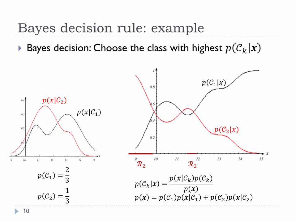
Bayes decision rule: example
10
} Bayes decision: Choose the class with highest 𝑝 𝒞$ 𝒙
𝑝(𝑥|𝒞,)𝑝(𝑥|𝒞2)
𝑝 𝒞, =23
𝑝 𝒞2 =13
𝑝(𝒞,|𝑥)
𝑝(𝒞2|𝑥)
ℛ2 ℛ2
𝑝 𝒞$ 𝒙 =𝑝 𝒙|𝒞$ 𝑝(𝒞$)
𝑝(𝒙)𝑝 𝒙 = 𝑝 𝒞, 𝑝 𝒙 𝒞, + 𝑝 𝒞2 𝑝 𝒙 𝒞2

Bayesian decision rule
11
} If 𝑃 𝒞,|𝒙 > 𝑃(𝒞2|𝒙) decide 𝒞,} otherwise decide 𝒞2
} If X 𝒙|𝒞N ](𝒞N)X(𝒙)
> X 𝒙|𝒞P ](𝒞P)X(^)
decide 𝒞,} otherwise decide 𝒞2
} If 𝑝 𝒙|𝒞, 𝑃(𝒞,) > 𝑝 𝒙|𝒞2 𝑃(𝒞2) decide 𝒞,} otherwise decide 𝒞2
Equivalent
Equivalent

Bayes decision rule: example
12
} Bayes decision: Choose the class with highest 𝑝 𝒞$ 𝒙
𝑝(𝑥|𝒞,)𝑝(𝑥|𝒞2)
𝑝 𝒞, =23
𝑝 𝒞2 =13
𝑝(𝒞,|𝑥)
𝑝(𝒞2|𝑥)
ℛ2 ℛ2
ℛ2 ℛ2
2×𝑝(𝑥|𝒞,)

Bayes Classier
13
} Simple Bayes classifier: estimate posterior probability ofeach class
} What should the decision criterion be?} Choose class with highest 𝑝 𝒞$ 𝒙
} The optimal decision is the one that minimizes theexpected number of mistakes

Diabetes example
14
} white blood cell count
This example has been adopted from Sanja Fidler’s slides, University of Toronto, CSC411

Diabetes example
15
} Doctor has a prior 𝑝 𝑦 = 1 = 0.2} Prior: In the absence of any observation, what do I know about
the probability of the classes?
} A patient comes in with white blood cell count 𝑥
} Does the patient have diabetes 𝑝 𝑦 = 1|𝑥 ?} given a new observation, we still need to compute the
posterior

Diabetes example
16 This example has been adopted from Sanja Fidler’s slides, University of Toronto, CSC411
𝑝 𝑥 𝑦 = 0
𝑝 𝑥 𝑦 = 1
𝑝 𝑥 = 40|𝑦 = 0 𝑃 𝑦 = 0 >? 𝑝 𝑥 = 40|𝑦 = 1 𝑃(𝑦 = 1)

Estimate probability densities from data
17
} If we assume Gaussian distributions for 𝑝(𝑥|𝑦 = 0) and𝑝(𝑥|𝑦 = 1)
} Recall that for samples {𝑥 , , … , 𝑥 d }, if we assume aGaussian distribution, the MLE estimates will be

Diabetes example
18 This example has been adopted from Sanja Fidler’s slides, University of Toronto, CSC411
𝑝 𝑥 𝑦 = 1 = 𝑁 𝜇,, 𝜎,2 𝜇, =∑ 𝑥(h)h:G(j)+,
∑ 1h:G(j)+,
=∑ 𝑥(h)h:G(j)+,
𝑁,
𝜎,2 =∑ ^ j klN
Pj:m(j)nN
dN
𝑝 𝑥 𝑦 = 0
𝑝 𝑥 𝑦 = 1

Diabetes example
19
} Add a second observation: Plasma glucose value
This example has been adopted from Sanja Fidler’s slides, University of Toronto, CSC411

Generative approach for this example
20
} Multivariate Gaussian distributions for 𝑝(𝑥|𝒞$):𝑝 𝒙 𝑦 = 𝑘
=1
2𝜋 p/2 Σ ,/2 exp{−12 𝒙 − 𝝁$ v𝜮$k, 𝒙 − 𝝁$ }
𝑘 = 1,2
} Prior distribution 𝑝(𝑦):} 𝑝 𝑦 = 1 = 𝜋, 𝑝 𝑦 = 0 = 1 − 𝜋

MLE for multivariate Gaussian
21
} For samples {𝑥 , , … , 𝑥 d }, if we assume a multivariateGaussian distribution, the MLE estimates will be:
𝝁 =∑ 𝒙(h)dh+,𝑁
𝜮 =1𝑁x 𝒙(h) − 𝝁 𝒙(h) − 𝝁 vd
h+,

Generative approach: example
22
Maximum likelihood estimation (𝐷 = 𝒙 h , 𝑦 hh+,d
):
} 𝜋 = dNd
} 𝝁, =∑ G(j)𝒙(j)zjnN
dN,𝝁2 =
∑ (,kG(j))𝒙(j)zjnN
dP
} 𝜮, =,dN∑ 𝑦(h) 𝒙(h) − 𝝁 𝒙(h) − 𝝁 vdh+,
} 𝜮2 =,dP∑ (1 − 𝑦 h ) 𝒙(h) − 𝝁 𝒙(h) − 𝝁 vdh+,
𝑁, = x𝑦(h)d
h+,
𝑁2 = 𝑁 − 𝑁,
𝑦 ∈ {0,1}

Decision boundary for Gaussian Bayes classifier
23
𝑝 𝒞, 𝒙 = 𝑝(𝒞2|𝒙)
ln 𝑝(𝒞,|𝒙) = ln 𝑝(𝒞2|𝒙)
ln 𝑝(𝒙|𝒞,) + ln 𝑝(𝒞,) − ln 𝑝(𝒙)= ln 𝑝(𝒙|𝒞2) + ln 𝑝(𝒞2) − ln 𝑝(𝒙)
ln 𝑝(𝒙|𝒞,) + ln 𝑝(𝒞,) = ln 𝑝(𝒙|𝒞2) + ln 𝑝(𝒞2)
ln 𝑝(𝒙|𝒞$)
= −𝑑2 ln 2𝜋 −
12 ln 𝜮$
k, −12 𝒙 − 𝝁$ v𝜮$k, 𝒙 − 𝝁$
𝑝 𝒞$ 𝒙 = X 𝒙|𝒞Y X(𝒞Y)X(𝒙)

Decision boundary
24
𝑝(𝒙|𝐶,) 𝑝(𝒙|𝐶2)
𝑝(𝐶,|𝒙)
𝑝(𝐶,|𝒙)=𝑝(𝐶2|𝒙)

Discriminant functions: Gaussian class conditional density
25
} Quadratic discriminant function is obtained.
𝑓} 𝒙 = 𝒙v𝑨}𝒙 + 𝒃}v𝒙 + 𝑐}𝑨} = −
12𝜮}
k,
𝒃} = 𝜮}k,𝝁}𝑐} = −
12𝝁}
v𝜮}k,𝝁} −12 ln 𝜮}
k, + ln 𝑃(𝒞})
} The decision surfaces are hyper-quadrics:} Hyper-planes, pairs of hyper-planes, hyper-spheres, hyper-
ellipsoids, hyper-paraboloids, hyper-hyperboloids

Shared covariance matrix
26
} When classes share a single covariance matrix 𝜮 = 𝜮,= 𝜮2
𝑝 𝒙 𝐶$ =1
2𝜋 p/2 Σ ,/2 exp{−12 𝒙 − 𝝁$ v𝜮k, 𝒙 − 𝝁$ }
𝑘 = 1,2
} 𝑝 𝐶, = 𝜋, 𝑝 𝐶2 = 1 − 𝜋

Likelihood
27
�𝑝(𝒙 h , 𝑦(h)|𝜋, 𝝁,, 𝝁2, 𝜮)d
h+,
=�𝑝(𝒙 h |𝑦 h , 𝝁,, 𝝁2, 𝜮)𝑝(𝑦 h |𝜋)d
h+,
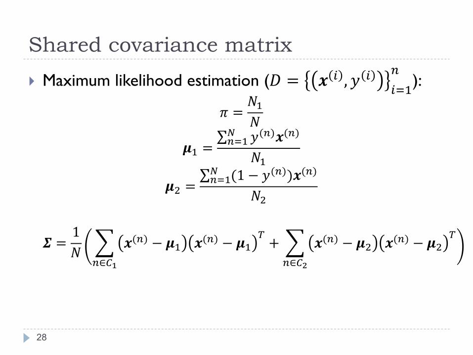
Shared covariance matrix
28
} Maximum likelihood estimation (𝐷 = 𝒙 } , 𝑦 }}+,h
):
𝜋 =𝑁,𝑁
𝝁, =∑ 𝑦(h)𝒙(h)dh+,
𝑁,
𝝁2 =∑ (1 − 𝑦(h))𝒙(h)dh+,
𝑁2
𝜮 =1𝑁 x 𝒙(h) − 𝝁, 𝒙(h) − 𝝁,
v�
h∈�N
+ x 𝒙(h) − 𝝁2 𝒙(h) − 𝝁2v
�
h∈�P

Decision boundary when shared covariance matrix
29
ln 𝑝(𝒙|𝒞,) + ln 𝑝(𝒞,) = ln 𝑝(𝒙|𝒞2) + ln 𝑝(𝒞2)
ln 𝑝(𝒙|𝒞$)
= −𝑑2 ln 2𝜋 −
12 ln 𝜮$
k, −12 𝒙 − 𝝁$ v𝜮k, 𝒙 − 𝝁$

Discriminant functions: Gaussian class conditional density with 𝜮, = 𝜮2 = 𝜮
30
} Linear discriminant function: 𝑓} 𝒙 = 𝒘}v𝒙 + 𝑤}�
} 𝒘} = 𝜮k,𝝁}} 𝑤}� = − ,
2𝝁}v𝜮k,𝝁} + ln 𝑃(𝒞})
} The decision hyper-plane between ℛ} and ℛ�:} 𝑓} 𝒙 − 𝑓� 𝒙 = 0 = 𝒘v𝒙 + 𝒘�
} 𝒘 = 𝜮k,(𝝁} − 𝝁�)
} 𝒘� = −,2𝝁,v𝜮k,𝝁, +
,2𝝁2v𝜮k,𝝁2 − ln
](𝒞�)](𝒞�)
This hyper-plane is not orthogonal to 𝝁}− 𝝁� linking the means

Bayes decision ruleMulti-class misclassification rate
31
} Multi-class problem: Probability of error of Bayesiandecision rule} Simpler to compute the probability of correct decision
𝑃 𝑒𝑟𝑟𝑜𝑟 = 1 − 𝑃(𝑐𝑜𝑟𝑟𝑒𝑐𝑡)
ℛ} : the subset of feature space assigned to the class 𝒞} using the classifier
𝑃 𝐶𝑜𝑟𝑟𝑒𝑐𝑡 =xM 𝑝(𝒙, 𝒞})ℛ�
*
}+,
𝑑𝒙
= xM 𝑝 𝒞} 𝒙 𝑝(𝒙)ℛ�
*
}+,
𝑑𝒙

Bayes minimum error
32
} Bayes minimum error classifier:
minQ(.)
𝐸𝒙,G 𝐼(𝛼(𝒙) ≠ 𝑦)
𝛼 𝒙 = argmaxG
𝑝(𝑦|𝒙)
Zero-one loss

Minimizing Bayes risk (expected loss)
33
for each 𝒙 minimize it that is called conditional risk
𝐸𝒙,G 𝐿 𝛼 𝒙 , 𝑦
= Mx𝐿 𝛼 𝒙 , 𝒞� 𝑝 𝒙, 𝒞� 𝑑𝒙*
�+,
�
�
= M𝑝 𝒙 x𝐿 𝛼 𝒙 , 𝒞� 𝑝 𝒞�|𝒙 𝑑𝒙*
�+,
�
�
} Bayes minimum loss (risk) decision rule: 𝛼�(𝒙)
𝛼�(𝒙) = argmin}+,,…,*
x𝐿}�𝑝 𝒞�|𝒙*
�+,The loss of assigning a sample to 𝒞} where the correct class is 𝒞�

Minimizing expected loss: special case(loss = misclassification rate)} Problem definition for this special case:
} If action 𝛼 𝒙 = 𝑖 is taken and the true category is 𝒞𝑗 , then thedecision is correct if 𝑖 = 𝑗 and otherwise it is incorrect.} Zero-one loss function:
𝐿}� = 1 − 𝛿}� = 00𝑖 = 𝑗1𝑜. 𝑤.
𝛼� 𝒙 = argmin}+,,…,*
x𝐿}�𝑝 𝒞�|𝒙*
�+,
= argmin}+,,…,*
0×𝑝 𝒞}|𝒙 +x𝑝 𝒞�|𝒙�
��}
= argmin}+,,…,*
1 − 𝑝 𝒞}|𝒙 = argmax}+,,…,*
𝑝 𝒞}|𝒙
34

Probabilistic discriminant functions
35
} Discriminant functions: A popular way of representinga classifier} A discriminant function 𝑓} 𝒙 for each class 𝒞} (𝑖 = 1,… , 𝐾):
} 𝒙 is assigned to class 𝒞} if:
𝑓𝑖(𝒙) > 𝑓𝑗(𝒙)"𝑗¹𝑖
} Representing Bayesian classifier using discriminantfunctions:} Classifier minimizing error rate: 𝑓𝑖 𝒙 = 𝑃(𝒞}|𝒙)} Classifier minimizing risk: 𝑓𝑖 𝒙 = −∑ 𝐿}�𝑝 𝒞�|𝒙*
�+,

Naïve Bayes classifier
36
} Generative methods} High number of parameters
} Assumption: Conditional independence
𝑝 𝒙 𝐶$ = 𝑝 𝑥, 𝐶$ ×𝑝 𝑥2 𝐶$ ×⋯×𝑝 𝑥p 𝐶$

Naïve Bayes classifier
37
} In the decision phase, it finds the label of 𝒙 according to:
argmax$+,,…,*
𝑝 𝐶$ 𝒙
argmax$+,,…,*
𝑝(𝐶$)�𝑝(𝑥}|𝐶$)h
}+,
𝑝 𝒙 𝐶$ = 𝑝 𝑥, 𝐶$ ×𝑝 𝑥2 𝐶$ ×⋯×𝑝 𝑥p 𝐶$
𝑝 𝐶$ 𝒙 ∝ 𝑝(𝐶$)�𝑝(𝑥}|𝐶$)h
}+,

Naïve Bayes classifier
38
} Finds 𝑑 univariate distributions 𝑝 𝑥, 𝐶$ ,⋯ , 𝑝 𝑥p 𝐶$ insteadof finding one multi-variate distribution 𝑝 𝒙 𝐶$} Example 1: For Gaussian class-conditional density 𝑝 𝒙 𝐶$ , it finds 𝑑 + 𝑑 (mean
and sigma parameters on different dimensions) instead of 𝑑 + p(p�,)2
parameters
} Example 2: For Bernoulli class-conditional density 𝑝 𝒙 𝐶$ , it finds 𝑑 (meanparameters on different dimensions) instead of 2� − 1parameters
} It first estimates the class conditional densities𝑝 𝑥, 𝐶$ ,⋯ , 𝑝 𝑥p 𝐶$ and the prior probability 𝑝(𝐶$) foreach class (𝑘 = 1,… , 𝐾) based on the training set.

Naïve Bayes: discrete example
39
} 𝑝 𝐻 = 𝑌𝑒𝑠 = 0.3
} 𝑝 𝐷 = 𝑌𝑒𝑠 𝐻 = 𝑌𝑒𝑠 = ,�
} 𝑝 𝑆 = 𝑌𝑒𝑠 𝐻 = 𝑌𝑒𝑠 = 2�
} 𝑝 𝐷 = 𝑌𝑒𝑠 𝐻 = 𝑁𝑜 = 2�
} 𝑝 𝑆 = 𝑌𝑒𝑠 𝐻 = 𝑁𝑜 = 2�
} Decision on 𝒙 = [𝑌𝑒𝑠, 𝑌𝑒𝑠] (a person that has diabetes and also smokes):} 𝑝 𝐻 = 𝑌𝑒𝑠 𝒙 ∝ 𝑝 𝐻 = 𝑌𝑒𝑠 𝑝 𝐷 = 𝑦𝑒𝑠 𝐻 = 𝑌𝑒𝑠 𝑝 𝑆 = 𝑦𝑒𝑠 𝐻 = 𝑌𝑒𝑠 = 0.066} 𝑝 𝐻 = 𝑁𝑜 𝒙 ∝ 𝑝 𝐻 = 𝑁𝑜 𝑝 𝐷 = 𝑦𝑒𝑠 𝐻 = 𝑁𝑜 𝑝 𝑆 = 𝑦𝑒𝑠 𝐻 = 𝑁𝑜 = 0.057} Thus decide 𝐻 = 𝑦𝑒𝑠
Diabetes (D)
Smoke (S)
Heart Disease (H)
Y N Y
Y N N
N Y N
N Y N
N N N
N Y Y
N N N
N Y Y
N N N
Y N N

Probabilistic classifiers
40
} How can we find the probabilities required in the Bayesdecision rule?
} Probabilistic classification approaches can be divided intwo main categories:} Generative
} Estimate pdf 𝑝(𝒙, 𝒞$) for each class 𝒞$ and then use it to find𝑝(𝒞$|𝒙)¨ or alternatively estimate both pdf 𝑝(𝒙|𝒞$) and 𝑝 𝒞$ to find 𝑝(𝒞$|𝒙)
} Discriminative} Directly estimate 𝑝(𝒞$|𝒙) for each class 𝒞$

Generative approach
41
} Inference stage} Determine class conditional densities 𝑝(𝒙|𝒞$) and priors𝑝(𝒞$)
} Use the Bayes theorem to find 𝑝(𝒞$|𝒙)
} Decision stage: After learning the model (inference stage),make optimal class assignment for new input} if 𝑝 𝒞} 𝒙 > 𝑝 𝒞� 𝒙 ∀𝑗 ≠ 𝑖 then decide 𝒞}

Discriminative vs. generative approach
42 [Bishop]

Class conditional densities vs. posterior
43
𝑝 𝒙 𝐶, 𝑝 𝒙 𝐶2𝑝 𝐶, 𝒙
𝑝 𝒞, 𝒙 = 𝜎(𝒘v𝒙 + 𝑤�)
𝒘 = 𝜮k, 𝝁, − 𝝁2𝑤� = −
12𝝁,
v𝜮k,𝝁, +12𝝁2
v𝜮k,𝝁2 + ln𝑝(𝒞,)𝑝(𝒞2)
[Bishop]
𝜎 𝑧 =1
1 + exp(𝑧)

Discriminative approach
44
} Inference stage} Determine the posterior class probabilities 𝑃(𝒞$|𝒙) directly
} Decision stage: After learning the model (inference stage),make optimal class assignment for new input} if 𝑃 𝒞} 𝒙 > 𝑃 𝒞� 𝒙 ∀𝑗 ≠ 𝑖 then decide 𝒞}

Discriminative approach: logistic regression
45
} More general than discriminant functions:} 𝑓 𝒙;𝒘 predicts posterior probabilities 𝑃 𝑦 = 1 𝒙
𝑓 𝒙;𝒘 = 𝜎(𝒘v𝒙)
𝜎 . is an activation function
} Sigmoid (logistic) function
𝜎 𝑧 =1
1 + 𝑒k£
𝐾 = 2
𝒙 = 1, 𝑥,, … , 𝑥p𝒘 = 𝑤�, 𝑤,, … , 𝑤p

Logistic regression
46
} 𝑓 𝒙;𝒘 : probability that 𝑦 = 1 given 𝒙 (parameterized by 𝒘)
𝑃 𝑦 = 1 𝒙,𝒘 = 𝑓 𝒙;𝒘
𝑃 𝑦 = 0 𝒙,𝒘 = 1 − 𝑓 𝒙;𝒘
} Example: Cancer (Malignant, Benign)} 𝑓 𝒙;𝒘 = 0.7} 70% chance of tumor being malignant
𝐾 = 2𝑦 ∈ {0,1}
𝑓 𝒙;𝒘 = 𝜎(𝒘v𝒙)0 ≤ 𝑓 𝒙;𝒘 ≤ 1estimated probability of 𝑦 = 1 on input 𝑥

Logistic regression: Decision surface
47
} Decision surface 𝑓 𝒙;𝒘 = constant} 𝑓 𝒙;𝒘 = 𝜎 𝒘v𝒙 = ,
,�¨©(𝒘ª𝒙)= 0.5
} Decision surfaces are linear functions of 𝒙
} if 𝑓 𝒙;𝒘 ≥ 0.5 then 𝑦 = 1} else 𝑦 = 0
Equivalent to
} if 𝒘v𝒙 + 𝑤� ≥ 0 then 𝑦 = 1} else 𝑦 = 0

Logistic regression: ML estimation
48
} Maximum (conditional) log likelihood:
𝒘¬ = argmax𝒘
log�𝑝 𝑦(}) 𝒘, 𝒙(})h
}+,
𝑝 𝑦(}) 𝒘, 𝒙(}) = 𝑓 𝒙(}); 𝒘 G(�) 1 − 𝑓 𝒙(}); 𝒘(,kG(�))
log 𝑝 𝒚 𝑿,𝒘
=x 𝑦(})log 𝑓 𝒙(}); 𝒘 + (1 − 𝑦(}))log 1 − 𝑓 𝒙(}); 𝒘h
}+,

Logistic regression: cost function
49
𝒘¬ = argmin𝒘
𝐽(𝒘)
𝐽 𝒘 = −x log 𝑝 𝑦(}) 𝒘, 𝒙(𝒊)h
}+,
=x−𝑦(})log 𝑓 𝒙(}); 𝒘 − (1 − 𝑦(}))log 1 − 𝑓 𝒙(}); 𝒘h
}+,
} No closed form solution for
𝛁𝒘 𝐽(𝒘) = 0} However 𝐽(𝒘) is convex.

Logistic regression: Gradient descent
50
𝒘²�, = 𝒘² − 𝜂𝛻𝒘𝐽(𝒘²)
𝛻𝒘𝐽 𝒘 =x 𝑓 𝒙 } ;𝒘 − 𝑦 } 𝒙 }h
}+,
} Is it similar to gradient of SSE for linear regression?
𝛻𝒘𝐽 𝒘 =x 𝒘v𝒙 } − 𝑦 } 𝒙 }h
}+,

Logistic regression: loss function
51
Loss 𝑦, 𝑓 𝒙;𝒘 = −𝑦×log 𝑓 𝒙;𝒘 − (1 − 𝑦)×log(1 − 𝑓 𝒙;𝒘 )
Loss 𝑦, 𝑓 𝒙;𝒘 = 0−log(𝑓(𝒙;𝒘)) if𝑦 = 1
−log(1 − 𝑓 𝒙;𝒘 ) if𝑦 = 0
How is it related to zero-one loss?
Loss 𝑦, 𝑦� = 01 𝑦 ≠ 𝑦�0 𝑦 = 𝑦�
𝑓 𝒙;𝒘 =1
1 + 𝑒𝑥𝑝(−𝒘v𝒙)
Since 𝑦 = 1 or 𝑦 = 0 ⇒

Logistic regression: cost function (summary)
52
} Logistic Regression (LR) has a more proper cost function forclassification than SSE and Perceptron
} Why is the cost function of LR also more suitable than?
𝐽 𝒘 =1𝑛x 𝑦 } − 𝑓 𝒙 } ;𝒘
2h
}+,
} where 𝑓 𝒙;𝒘 = 𝜎(𝒘v𝒙)} The conditional distribution 𝑝 𝑦|𝒙,𝒘 in the classification problem is
not Gaussian (it is Bernoulli)} The cost function of LR is also convex

Posterior probabilities
53
} Two-class: 𝑝 𝒞$ 𝒙 can be written as a logistic sigmoid fora wide choice of 𝑝 𝒙 𝒞$ distributions
𝑝 𝒞, 𝒙 = 𝜎 𝑎(𝒙) =1
1 + exp(−𝑎(𝒙))
} Multi-class: 𝑝 𝒞$ 𝒙 can be written as a soft-max for awide choice of 𝑝 𝒙 𝒞$
𝑝 𝒞$ 𝒙 =exp(𝑎$(𝒙))
∑ exp(𝑎�(𝒙))*�+,

Multi-class logistic regression
54
} For each class 𝑘, 𝑓$ 𝒙;𝑾 predicts the probability of 𝑦 = 𝑘} i.e.,𝑃(𝑦 = 𝑘|𝒙,𝑾)
} On a new input 𝒙, to make a prediction, pick the class thatmaximizes 𝑓$ 𝒙;𝑾 :
𝛼 𝒙 = argmax$+,,…,*
𝑓$ 𝒙
if 𝑓$ 𝒙 > 𝑓� 𝒙 ∀𝑗 ≠ 𝑘 thendecide 𝐶$

Multi-class logistic regression
55
𝐾 > 2𝑦 ∈ {1,2, … , 𝐾}
𝑓$ 𝒙;𝑾 = 𝑝 𝑦 = 𝑘 𝒙 =exp(𝒘$
v𝒙 )∑ exp(𝒘�v𝒙 )*�+,
} Normalized exponential (aka softmax)} If 𝒘$
v𝒙 ≫ 𝒘�v𝒙 for all 𝑗 ≠ 𝑘 then 𝑝(𝐶$|𝒙) ≃ 1, 𝑝(𝐶�|𝒙) ≃ 0
𝑝 𝐶$ 𝒙 =𝑝 𝒙 𝐶$ 𝑝(𝐶$)
∑ 𝑝 𝒙 𝐶� 𝑝(𝐶�)*�+,
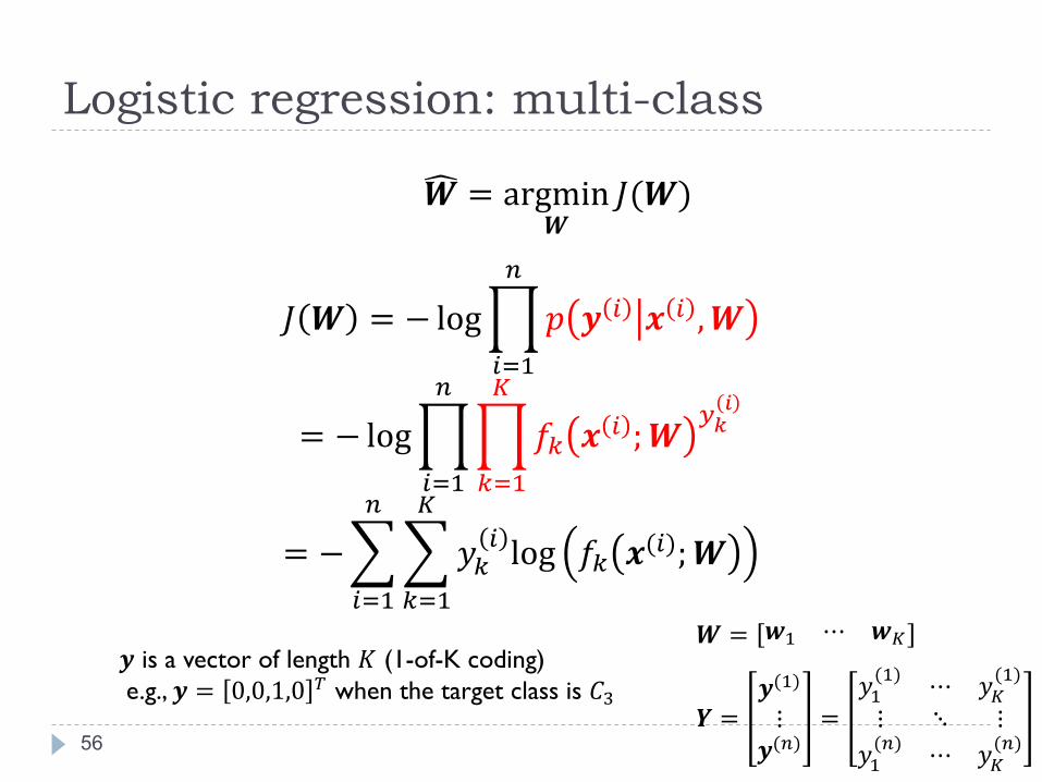
Logistic regression: multi-class
56
𝑾¼ = argmin𝑾
𝐽(𝑾)
𝐽 𝑾 = − log�𝑝 𝒚 } 𝒙 } ,𝑾h
}+,
= − log��𝑓$ 𝒙 } ;𝑾GY�
*
$+,
h
}+,
= −xx𝑦$} log 𝑓$ 𝒙(});𝑾
*
$+,
h
}+,𝑾 = 𝒘, ⋯ 𝒘*
𝒀 =𝒚(,)⋮
𝒚(h)=
𝑦,(,) ⋯ 𝑦*
(,)
⋮ ⋱ ⋮𝑦,(h) ⋯ 𝑦*
(h)
𝒚 is a vector of length 𝐾 (1-of-K coding)e.g., 𝒚 = 0,0,1,0 v when the target class is 𝐶�

Logistic regression: multi-class
57
𝒘�²�, = 𝒘�² − 𝜂𝛻𝑾𝐽(𝑾²)
𝛻𝒘�𝐽 𝑾 =x 𝑓� 𝒙 } ;𝑾 − 𝑦�} 𝒙 }
h
}+,

Logistic Regression (LR): summary
58
} LR is a linear classifier
} LR optimization problem is obtained by maximumlikelihood} when assuming Bernoulli distribution for conditional
probabilities whose mean is ,,�¨©(𝒘ª𝒙)
} No closed-form solution for its optimization problem} But convex cost function and global optimum can be found by
gradient ascent

Discriminative vs. generative: number of parameters
59
} 𝑑-dimensional feature space
} Logistic regression: 𝑑 + 1 parameters} 𝒘 = (𝑤�,𝑤,, . . , 𝑤p)
} Generative approach:} Gaussian class-conditionals with shared covariance matrix
} 2𝑑 parameters for means} 𝑑(𝑑 + 1)/2 parameters for shared covariance matrix} one parameter for class prior 𝑝(𝐶,).
} But LR is more robust, less sensitive to incorrect modelingassumptions

Summary of alternatives
60
} Generative} Most demanding, because it finds the joint distribution 𝑝(𝒙, 𝒞$)} Usually needs a large training set to find 𝑝(𝒙|𝒞$)} Can find 𝑝(𝒙) ⇒ Outlier or novelty detection
} Discriminative} Specifies what is really needed (i.e., 𝑝(𝒞$|𝒙))} More computationally efficient

Resources
61
} C. Bishop, “Pattern Recognition and Machine Learning”,Chapter 4.2-4.3.