This PDF is a selection from an out-of-print volume from the National Bureauof Economic Research

Volume Title: Shares of Upper Income Groups in Income and Savings

Volume Author/Editor: Simon Kuznets, assisted by Elizabeth Jenks

Volume Publisher: NBER

Volume ISBN: 0-87014-054-X

Volume URL: http://www.nber.org/books/kuzn53-1

Publication Date: 1953

Chapter Title: Shares of Upper Income Groups in Savings

Chapter Author: Simon Kuznets, Elizabeth Jenks

Chapter URL: http://www.nber.org/chapters/c3060

Chapter pages in book: (p. 171 - 218)

Part III

Income and Savings

S

C

Chapter 6

SHARES OF UPPER INCOME GROUPS TN SAVINGS

1 Setting of the ProblemDistribution of income by size is of importance in so far as it affects theproductivity of the various income classes in turning out the country'stotal product, determines how people use their income, and measures theeconomy's contribution to the well-being of the several groups in society.To trace these consequences of the income distribution would be difficultand we do not attempt it even for the shares of upper income groups. Thediscussion that follows is concerned with only one of the many uses towhich data on upper group shares can be applied: an analysis of the effecton savings.

Interest in the apportionment of income between consumption expendi-tures and savings has been intensified by the strategic role Keynesian theoryhas assigned to it in influencing cyclical fluctuations and, on some inter-pretations, trends; moreover, the great depression of the 193 0's heightenedconcern as to how well our economy satisfies the needs of various con-sumer groups. As a result, several countrywide studies of income, con-sumer expenditures, and savings, by income size classes, have been made.We can therefore, albeit with some difficulty, study upper group shares inindividuals' total savings, relating their level and changes to the level ofand changes in shares in income.

The data do not yield adequate annual estimates of even total savingsof individuals, let alone savings of upper separately from those of lowerincome groups. Hence, to derive at least reasonable hypotheses concern-ing the level of, and particularly short term changes in, upper group sharesin individuals' total savings, we must analyze the sample data on savingsfor the various income size classes.

But first it may be helpful to explore the formal relations between sharesin income and in savings. Defining upper groups as we have done through-out this study — as the top 5 percent in a classification by current incomeper capita — we call the percentage of income received by it The aver-age level of in the economic income variant was about 30 percent during1919-38. The income share of the lower groups may be designated andsince + 1, its average level was about 70 percent.

The percentage shares of upper and lower income groups in individuals'

173

174 PART IIItotal savings are and The relation between and (orbetween and S1) depends upon the proportion of their income units atupper (or lower) income levels save. If we call the savings-income ratiofor upper and lower groups and respectively and the savings-incomeratio for all individuals the following simple relations can be stated:

(1)

(2)

(3)and

(4)

These equations show that if we wish to study the level of and changesin (and S1) we need to know not only (and Ii), which we studied inthe preceding chapters, but also andRe (or alternatively, R1 and or

and Ri). Information regarding the savings-income' ratios for uppergroups and for all groups (or for upper and for lower groups) is thus indis-pensable if we are to learn anything about upper group shares in individ-uals' total savings.

The average level of one of these ratios, can be approximated fromthe sample studies analyzed in detail in Section 3. Let us accept this aver-age level and, in order to demonstrate the effects of changes in alone,assume that is constant, i.e., does not change during the period understudy. Observation of these effects, together with what we know about themovement of the ratio of individuals' total savings to their total income,

will lead us to formulate the specific question our study of andshould answer.

Calculations based on this assumption appear in Table 47, columns1-11 where we associate the positions of income groups, i.e., their incomemultiples, described below, with the savings-income ratios assumed forthose positions, specific RtL's. These ratios can be studied for either (a)given percentile groups, i.e., the top 1, 5, etc. percent of the populationin each year, or (b) groups at given relative income levels or incomemultiple positions, i.e., groups that in each year derive incomes x timesthe average income per capita. Measures under (a) would be more directlyrelevant to the analysis. But the sample data on expenditures and savingsyield more reliable estimates of savings-income ratios for (b). For thisreason we couch Table 47 largely in terms of savings-income ratios atincome multiple positions.

In columns 1, 4, and 7 we record the percentage shares in total income(economic income variant) received by the three upper groups. When

CHAPTER 6 175

related to the percentage of the population covered, these shares determinefor each year the income multiple position of each group; e.g., in 1919 theincome multiple position of the top 1 percent was 14.0; of the 2nd and 3rdpercentage band, 3.4. From the scattered sample evidence on expendituresand savings summarized in Section 3 (excluding that for 1948-50, whichbecame available later) we estimate the savings-income ratio correspond-ing to the given income multiple position on the assumption that its levelis constant for the period covered in Table 47 (col. 2, 5, and 8). Multiply-ing their income shares by their savings-income ratios, we obtain thehypothetical savings of the three upper groups, expressed in percentages ofindividuals' total income (col. 3, 6, and 9). The sum of these estimates forthe three upper groups gives the savings of the top 5 percent (col. 10).

What would their hypothetical savings be if we assumed that the savings-income ratio is constant for a given percentile group instead of for a givenincome multiple position? This assumption can easily be applied by usingin columns 2, 5, and 8 a constant instead of a changing savings-incomeratio. Setting the constant savings-income ratio for a given group at itsmean level for the period, calculating the product of this ratio and thegroup's share, and adding the products for the three groups, we get column11: the hypothetical savings of the top 5 percent group, expressed in per-centages of individuals' total income, on the assumption that the savings-income ratio for a given upper percentage band is constant.

In interpreting the results, two cautions must be kept in mind. First,when we convert the average per capita income of an income group (say,the top 1 percent) to an income multiple we identify that group with anincome point. But the significance of a given multiple as a factor determin-ing a savings-income ratio may depend upon the income from whichit was derived. Thus the multiple 3 calculated from a range of incomesextending from the multiple 10 down to 0.5 may yield one savings-incomeratio; and the multiple. 3 calculated from a range of incomes from 3.1down to 2.9, a somewhat different ratio. Hence, there is an element ofarbitrariness in passing from income groups to multiples. However, at thehigh income levels treated, here, where the curve of savings-income ratiostends to be asymptotic to a constant or only slowly rising line of ratios, thepossible error cannot be large.

The second caution relates to the savings-income ratios. Those yieldedby the sample studies of expenditures and savings are usually higher thanthose yielded by the residual method which employs over-all totals orother approaches. Therefore, the savings-income ratios assumed for themultiples in Table 47 may be somewhat too high, even for the underlyingconcept of savings, i.e., including depreciation on consumer durable goods

Table 47

Savings of Upper Income Groups as Percentages of Individuals' Total IncomeReceipts, Assuming Constant Savings-Income Ratios for Given Upper IncomeLevels, 1919-1945

TOP 1 PERCENT 2ND & 3iu PERCENTAGE BAND% Share % Sharein Total Savings in Total SavingsIncome, Savings- as % of Income, Savings- as % of

Economic Income Total Economic. Income TotalIncome Ratio Income Income Ratio IncomeVariant (%) (1) X (2) Variant (%) (4) X (5)

(1) (2) (3) (4) (5) (6)1919 14.0 42.10 5.9 6.8 25.80 1.71920 13.6 41.86 5.7 6.8 25.80 1.81921 16.2 43.06 7.0 9.0 29.46 2.71922 15.6 42.84 6.7 8.0 28.00 2.21923 14.0 42.10 5.9 8.5 28.60. 2.41924 14.7 42.48 6.2 8.4 28.60 2.41925 15,7 42.88 6.7 8.1 28.00 2.31926 15.8 42.92 6.8 8.2 28.30 2.31927 16.5 43.15 7.1 8.4 28.60 2.41928 17.2 43.34 7.4 8.3 28.30 2.31929 17.2 43.34 7.4 8.5 28.60 2.41930 15.6 42.84 6.7 8.4 28.60 2.41931 15.6 42.84 6.7 9.0 29.46 2.71932 15.3 42.72 6.5 9.3 30.01 2.81933 14.4 42.33 6.1 8.9 29.18 2.61934 13.6 41.86 5.7 8.5 28.89 2.51935 13.6 41.86 5.7 8.4 28.60 2.41936 14.7 42.48 6.2 8.0 28.00 2.21937 14.1 42.16 6.0 8.0 28.00 2.21938 12.8 41.38 5.3 8.4 28.60 2.41939 13.3 41.68 5.5 8.4 28.60 2.41940 13.0 41.50 5.4 7.8 27.70 2.21941 12.5 41.19 5.1 7.6 27.35 2.11942 10.8 39.84 4.3 6.8 25.80 1.81943 10.1 39.12 3.9 6.2 24.60 1.51944 9.1 37.92 3.4 5.8 23.40 1.41945 9.5 38.40 3.6 6.0 24.00 1.4

Column2, Multiples of average income were derived by dividing the percentage of5, income received (col. 1, 4, and 7) by the percentage of population receiv-8 ing it. To each multiple a savings-income ratio was assigned, set, on the

basis of the sample evidence for 1929, 1935-36, 1942 (first quarter),1945, 1946, and 1947 in Section 3, at 17 percent 'for the multiple 2, 24percent for the multiple 3, 28 percent for the multiple 4, 30.8 percent forthe multiple 5, 33.2 percent for the multiple 6, 35 percent for the multiple 7,37.8 percent for the multiple 9, 39 percent for the multiple 10, and 45 per-cent for the multiple 25, and interpolated with an allowance for decreasingincrements in the savings-income ratio as the multiple increases.

10 Sum of columns 3, 6, and 9.11 Sum of products of columns 1, 4, and 7 and a constant savings-income ratio.

The constant ratio for column 1, 41.859 percent, is the arithmetic mean ofcolumn 2 for 1919-45; that for column 4, 27.735 percent, the arithmeticmean of column 5; and that for column 7, 24.037 percent, the arithmeticmean of column 8.

12, a) To the NBER estimates of individuals' savings for 1919-38 (National13 income and its Composition, 1919-1938, Table 39, p. 276) and the Depart-

176

Rank of ShareTOP 5 PERCENT (Upward) of

4TH & STE PERCENTAGE BAND Savings as % of Top 5 Percent Group% Share Total Income in Total Savingsin Total Savings Assuming Constant Assuming ConstantIncome, Savings- as % of Savings-Income Ratio Savings-Income Ratio

EconOmic Income Total for Given for GivenIncome Ratio Income income Percentage income PercentageVariant (%) (7) X (8) multiple band multiple band

(7) (8) (9) (10) (11) (12) (13)5.3 21.60 1.1 8.8 9.0 6 65.3 21.60 1.1 8.6 8.9 10 106.5 25.40 1.7 11.3 10.8 26 266.8 25.80 1.7 10.7 10.4 20 205.6 22.80 1.3 9.6 9.6 12 126.0 24.00 1.4 10.1 9.9 19 196.4 25.00 1.6 10.6 10.4 14 146.3 24.60 1.5 10.6 10.4 18 186.3 25.00 1.6 11.1 10.7 17 176.6 25.40 1.7 11.5 11.1 21 216.2 . 24.60 1.5 11.4 11.0 15 156.7 25.40 1.7. 10.8 10.5 23. 237.4 27.00 2.0 11.3 10.8 22 227.5 27.35 2.1 11.4 10.8 24 247.6 27.35 2.1 10.7 10.3 27 277.1 26.20 1.9 10.0 9.7 25 256.8 25.80 1.8 9.8 9.6 13 136.5 25.40 1.7 10.2 10.0 8 86.4 25.00 1.6 9.8 9.7 11 116.6 25.40 1.7 9.4 9.3 16 166.4 25.00 1.6 9.5 9.4 9 96.3 24.60 1.5 9.1 9.1 7 75.9 23.40 1.4 8.6 8.7 5 55.1 21.00 1.1 7.1 7.6 3 34.8 20.30 1.0 6.4 7.1 2 24.0 17.00 0.7 5.5 6.4 . 1 1

4.0 17.00 0.7 5.8 6.6 4 4

ment of Commerce estimates of personal savings for 1929-45 (Survey ofCurrent Business, July 1949, Table 3, p. 10) was added the latter's serieson depreciation on owner-occupied dwellings as shown for 1929-41 in ibid.,July 1947, National Income Supplement, Table 39, p. 47, for 1942-45 inibid., July 1949, Table 39, p. 25, and extrapolated back to 1919 by an indexbased on depreciation on all residences (Solomon Fabricant, Capital Con-sumption and Adjustment, NBER, 1938, Table 29, p. 160) and the ratio ofimputed rent to all rent paid on urban dwellings as computed from dataunderlying the NBER series on total imputed rent.b) The series for 1919-38 and 1929-45 calculated in (a) were divided byaggregate payments to individuals including depreciation on owner-occu-pied dwellings from sources cited in (a).c) The percentages for 1919-38 and 1929-45 calculated in (b) were con-verted to indexes with 19 19-38 as the base.d) The index for 19 19-38 calculated in (c) was extrapolated through 1945by that for 1929-45.e) Columns 10 and 11, each converted to an index with 1919-38 as the base,were divided by the index for 1919-45 calculated in (d), and the ratiosranked in increasing order, to yield columns 12 and 13 respectively.

177

178 PART IIIand residential housing. However, here again a reasonable scaling downof the levels would not greatly affect the significance of the evidence.

The hypothetical savings of upper income groups, whether calculatedon the assumption that savings-income ratio is constant for a givenincome multiple position (col. 10) or for a given percentile group (col.11), expressed in percentages of individuals' total income, vary little exceptfor the years since 1939. Their slight fluctuations are counter-cyclical'(they rise in 1921 and 1924, decline in 1920 and 1923, and show practi-cally no decline during the great depression of 1929-33).

Columns 10 and 11 should be compared with individuals' total savings,also expressed in percentages of individuals' total income, i.e., butunfortunately, there is no reliable' series. Available series, derived by theresidual method, yield savings-income ratios whose average level is notconsistent with the evidence yielded by the samples summarized in Section3 and used in Table 47. But, for purposes of rough comparison, we tookindividuals' total savings derived crudely 'as the difference between aggre-gate income receipts and consumer expenditures plus taxes; added depre-ciation on owner-occupied houses; expressed the totals as percentages ofall income payments to individuals; converted these percentages to anindex with 1919-38 as the base; took the ratio of columns 10 and 11 (alsoconverted to indexes with 1919-38 as the base) to this index; and rankedthe ratios from lowest to highest.'

The share of the top 5 percent in total savings declined after 1939 and,what is more important here, its movement was counter-cyclical (col. 12and 13). The years of depression, 1921, 1924, 1932-33, and 1938, aremarked by high ranks, indicating a high.ratio of upper group to total sav-ings. The years of prosperity, 1919-20, 1923, 1929, and 1936-37, incontrast, are marked by low ranks.2

The question we propose to explore can now be posed. Is the assumptionunderlying Table 47 realistic: that the savings-income ratios for the upperincome positions or groups, move relatively little during the shortperiods associated with business cycles? If they are relatively stable in theshort run, the share of upper group savings in total savings, must varywidely and run counter to business cycles. Only if the savings-income ratiosfor upper income positions or groups vary with business cycles and much

1 We used ranks instead of the actual ratios because lack of confidence in the serieson individuals' total savings made the ratios suspect.2 There is some hint that the decline in the ratio of upper group to total savingsreaches a trough somewhat before the peak in general business conditions (in 1919rather than 1920, 1936 rather than 1937). But the data are too crude to reveal leadsor lags.

CHAPTER 6 179

more widely than those for lower income positions or groups will thisgreater variability of the former tend to offset the counter-cyclical move-ment of their income shares and make for a constant share in individuals'total savings. The question, then, reduces itself to one concerning the rela-tive short term variability of savings-income ratios for upper and lowergroups.

2 Effect of Changes in Savings-Income Ratios on Changesin Shares in Individuals' Total Savings

Before we study the sample data with an eye to the variability of savings-income ratios, let us explore the formal relations between changes in thesavings-income ratios, i.e., R1, and and in the shares in savings, i.e.,

and Such an analysis will indicate in what form we should comparethe variability of the savings-income ratios of upper and lower incomegroups respectively if we are to be able to draw unequivocal conclusionsconcerning changes in their shares in total savings.

a) Proportional changes in RWe begin with proportional changes in the savings-income ratios largelybecause they yield simpler results than absolute changes. Assume thatproportional changes in and in R1 are equal and expressible by a factorA. If for the initial point of time we retain the designations in equations(1)- (4) in Section 1, and for the next point of time at which the assumedchange is observed, we add a plus sign to the subscripts, we get:

(5)

=

______

== (6)

11R1A — —s 7'

As (6) and (7) show, the same proportional change in the savings-incomeratios for upper and lower income groups leaves their shares in savingsunaffected.

Assume now a proportional change in equal to A, and a proportionalchangeinR1equaltoB,whereB=A (1 +m).

(1+m)

=A

ARt(1+Sjm) (8)

180 PART III1 \_ ( 1

u+AR(1+Sm)_ (

11R1A(l+m) 1+m10

—(

As (9) and (10) show, different proportional changes the savings-income ratios of upper and lower income groups alter their shares in totalsavings. The proportional change in upper group shares in savings is mea-

sured by the ratio1 m

since it equals (from equation 9); and

that in the share of lower groups by1 + s1 m

(from equation 10).

Let us assume that S1 is positive, i.e., that the lower income groups dosave; and that m never becomes algebraically smaller than —1 (if it did,51+ would be negative). Under these reasonable assumptions, we can com-pare the proportional change in and S1 respectively with the relativedifference between A and B.

Su÷ Sl+

Line Signofm(1) (2) (3)

1 1 1±m1 Plus > <1+m1+S1m 1+m 1+S1m

1 1 1—rn2 Minus >1—rn

1—S1m 1—rn 1—S1m

Since S1 is necessarily a proper fraction, a positive m, i.e., a larger pro-

portional increase (or smaller decrease) in the ratio for lower incomegroups, increases their share in total savings and decreases that of uppergroups. But as can be seen from line 1, the proportional increase in thesavings share of lower income groups is smaller than (1 + m), i.e., thanthe relative difference between A and B. Likewise, when rn is negative,both the proportional increase in the share of upper income groups in totalsavings and the proportional decrease in that of lower groups are smallerthan the relative difference between A and B. The point note is thatthe analysis of proportional changes in the savings-income ratios for upperand for lower income groups does not suggest consistent differences in thesensitivity of their shares in total savings.

b) Absolute changes in RThe significance Of these conclusions becomes evident when we contrastthem with the effects of absolute changes in and R1.

Assume the same absolute change in and R1, and call it a. Then:

CHAPTER 6 181

+(11)

—12

—(

where a = k Rt

—Sz+_R(l+k) (13)

It follows that:

—(1 +k)

— (R

— —(14)

— — —

Likewise

— 11k( )

Equations (14) and (15) provide the key to the effects of absolutechanges in the savings-income ratios on the percentage shares of upperand lower income groups in total savings. It should be remembered that

is almost necessarily negative, and —. R1 positive. Conse-quently, if a (and hence k) is positive, — is negative, whereas

— S1 is positive. Likewise, when a (and hence k) is negative, —

is positive, whereas — S1 is negative. In other words, the same absoluteincrease in the savings-income ratio for upper and lower income groupscauses a decline in the former's share in total savings (and a correspondingrise in the latter's share), and the same absolute decline in the savings-income ratio for the upper and lower income groups causes a rise in theformer's share in total savings (and a corresponding decline in the latter'sshare).

This conclusion is unavoidable inasmuch as we have already observedthat only an equal proportional change in and leaves the savingsshares unaffected. But its significance for the analysis that follows warrantsspecial emphasis. Equality of absolute change in savings-income ratios

182 PART IIIdoes not mean temporal stability of and but rather a change inopposite in sign to that in both and R1. If the absolute changes inand R1 are in the same direction, as they tend to be during business cycles,their equality would still cause a change in upper group shares in totalsavings — a counter-cyclical change. Given the same direction of shortterm changes in and R1, only an equal proportional amplitude of varia-tions in and R1 would assure a short term constancy of and S1.

In the light of the sample evidence to be considered in Section 3 (andalready used in Table 47), for the upper income groups as we definethem is about 5 times as large as R1. It is, therefore, extremely unlikelythat proportional changes in can ever be as large as in R1.3 In otherwords, the smaller proportional variability of than of R1 is almost inthe nature of a mathematical necessity. Hence the empirical analysis of

and R1 is more in the way of measuring the difference in temporal varia-bility than of proving its existence.

3 Statistical Evidence on Savings-Income Ratiosa) Various samples, total populationWhat are the savings-income ratios at upper and at lower income levels?How do they change over time? To answer these questions we used theBrookings estimates for 1929; the Consumer Purchases Study for 1935-36;the Survey of Spending and Saving in Wartime for 1941 and the firstquarter of 1942; and the Surveys of Consumer Finances for 1945-50.Their important defects must be borne in mind in appraising the evidence.4

First, the sample studies underrepresent upper income groups in varyingdegree; and while in some this underrepresentation has been adjusted for,the empirical basis for measurement at the upper levels is slender. In short,for the very groups in whose income disposition we are most interested, thesample data are most limited.

• Second, with the possible exception of the 1935-36 study, the thinnessof the sample when distributed by size of income and by some other charac-

8 Since has an average level of 3 0-40 percent, it cannot rise much more than twiceas high; nor, in view of the large average income involved, is it likely to decline toa negative value. At lower income levels, where is well below 10 percent, theratio can easily rise to 2 or 3 times its average level and as easily drop to a negativevalue. With the decline in the income shares of upper groups in recent years, theirsavings-income ratio may be lower than the 30-40 percent cited above. But even so,it is high enough, and sufficiently higher than that for the lower groups for theconclusion in the text to hold.'For an analysis of the concept of savings in the first two studies, see also Nationalincome and its Composition, 1919-1938, pp. 292 if.

CHAPTER 6 183

teristic (e.g., by urban and rural areas or by family status) makes forirregularity of savings-income patterns.

Third, the years included do not represent a sufficient variety of cyclicalexperience. Indeed, in the Brookings analysis the income size distributionfor 1929 is combined with consumption-savings ratios derived from budgetstudies covering scattered years from 1918 to 1932. The other studies arebased on data for a specific year and none covers a year of marked cyclicaldepression or trough. Hence, while the years are not at the same stage ofcyclical expansion, all are above the cyclical trough and with rising incomes— and similar evidence for years of cyclical trough and with decliningincomes is not available, with the single exception of the mild recessionfrom 1948 to 1949. However, some light on savings-income ratios duringa period of decline in incomes is provided by the Brookings special samplefor 1928-32, discussed in Section 3c.

Fourth, the concept of income used does not correspond to that under-lying the national income total. The Brookings distributions are based onincome including gains and losses from sales of assets. In the ConsumerPurchases Study gifts and transfers from other individuals are included aswell as net profits from property bought and sold within the year. In theSurveys of Consumer Finances money income alone is included.

Fifth, the concept of savings does not correspond to the definition im-plied in national income measurement. In the Brookings study it is seri-ously affected by the inclusion of capital gains and losses. In practically allthe studies savings are gross of depreciation on owner-occupied dwellingsunless current expenses happen to exceed current maintenance by anamount equal to the allowable depreciation, and interest accruing to indi-viduals in such institutions as savings banks and life insurance companiesis omitted.

Sixth, the unit of classification for both income and savings varies fromstudy to study. The Brookings distribution is among families and singlepersons. The Consumer Purchases Study and the Survey of Spending andSaving in Wartime are in terms of consuming units which differ fromcensus families in. that they exclude members who do not pool their incomeand expenses. The Surveys of Consumer Finances are in terms of spendingunits, a concept that seems similar to that of consuming units in the1935-36 and 1941-42 studies, but it is not clear from the published datawhether the definitions coincide in detail.

We now consider how our attempt to compare the results of these sev-era! studies removes or reduces these defects and the incomparabilitiesarising from them. The several steps are described in the notes to the tables

184 PART IIIin Appendix 1; here only a minimum summary statement indispensablefor understanding the results is given.1) We tried to adjust the Brookings 1929 distribution to exclude gains andlosses on sales of assets. It was easy to approximate the results for thedistribution of income by size. But for savings, a problem arose to whiähwe had no ready answer. The savings-income ratios used in that study werederived by applying to the size classes of income including capital gainsand losses in 1929 proportions found in various budget studies. The under-lying budget studies, with the single exception of the Brookings specialsample for 1928-3 2, were all for incomes in which capital gains and losseswere negligible or excluded by definition. We can argue either that (a)consuming units enjoying such gains (or suffering such losses) considerthem as bona fide income (or losses) and permit them to affect fully theircurrent consumption and savings patterns (Assumption 1). Their truesavings can then be calculated by subtracting the estimated capital gainsand losses from the savings as estimated in. the Brookings study. Or wecan argue that (b) consuming units consider capital gains and losses aspurely transitory and do not permit them to affect their current consump-tion and savings patterns, in which case the latter would reflect incomeexcluding capital gains and losses (Assumption 2). We can, then, estimateincome excluding capital gains and losses at successive levels, and applythe savings-income ratios used in the Brookings study for identical levelsof income including gains and losses.

No attempt at other adjustments for the concept of either income orsavings was made.2) Because the studies vary in the degree to which they underrepresentupper income groups, direct comparison of the savings-income ratios forthe top 1 or 5 percent group in each would be misleading. The same toppercentage band in two studies would in fact be two different percentagebands in terms of the total population of the country. We therefore con-verted the income size classes in each study' to classes characterized byincome expressed as a multiple of the arithmetic mean income for the givensample study; then adjusted the multiples in each study by the relativediscrepancy between the total income shown by the study and that shownby comparable and continuous Department of Commerce series. Forexample, for 194 1-42 the family units with incomes of, say, $3,000-5,000,were first expressed as a class whose income was x times the average familyincome shown by the study; this x was then multiplied by 0.87, the ratioof total income covered by the study to the comparable Department ofCommerce total. Thus, the level of. each income size class in each study

CHAPTER 6 185

was measured relative to a comparable and continuous series derived fromthe Department of Commerce estimates of national income.5

This conversion of the income of a sample unit or class to a multiple orrelative of per unit income for the country not only serves to adjust forvarying degrees of underrepresentation but also expresses the income posi-tion of a unit or class in a more meaningful way than would the absolutedollar value of its income or its relative standing within the sample. Coun-trywide per unit income is, of course, a rather unrepresentative average.But it is near enough some norm or standard to give a unit that enjoys anincome x times it a meaningful relative position. For example, a $1,000income leads to one type of apportionment between expenditures and sav-ings when it is twice countrywide per unit income and to another when itequals the countrywide per unit income. Likewise, a position relative to acountrywide per unit income is more meaningful than a position within asample that may suffer from various biases. Without claiming too muchfor this conversion, one could reasonably argue that it is likely to lead to amore useful analysis of savings patterns than relating savings-income ratiosto absolute levels of dollar income or to relative positions within eachsample.

A final advantage of this conversion is that it makes possible the com-parison of the savings-income ratios derived from the samples with ourestimates of upper group shares in income, which were measured forgroups classified by their position relative to countrywide per capitaincome.3) Variation in the unit of count and classification could not be adjustedfor. But whenever possible, i.e., for all data except those in the Surveysof Consumer Finances, the family or consuming unit was reduced to a percapita basis and the entire calculation of relative income levels wasrepeated in terms of income per capita. The reduction was necessarilycrude but removed both an element of variability among the several studiesand an element that might obscure the savings-income patterns, viz., dif-ferences among units, classified by total income, in the number dependentupon that income.4) Irregularities in the savings-income ratios for the income classes abovethe lowest ranges in the Surveys of Consumer Finances appeared to be dueto the thinness of the samples. We therefore fitted simple straight lines tothe ratios (logarithms of income multiples compared with the ratio of theshare in savings to the share in income) for these income classes, and read

Elements of discontinuity still remained as far as the scope of intended coveragediffered among the studies. The most notable example is the limitation of the Surveysof Consumer Finances to money income.

186 PART IIIthe savings-income ratios from these lines instead of taking them directlyfrom the published data. A similar procedure might perhaps have beenused to advantage on the 1941-42 study, but the income classes were sofew that it did not seem worth while.

Obviously, we did not correct all the major defects of the studies, norcould we. The notable defects that still remain are: the limitation of theSurveys of Consumer Finances to money income; the use of a concept ofsavings gross of depreciation on owner-occupied dwellings; absence ofdata for years of declining income and cyclical trough; absence or thinnessof sample data for upper income groups.

Table 48 covers all the samples and shows the percentage that savingsare of income for consuming or spending units classified by the ratio oftheir income to the per unit income for the country as a whole derivedfrom the Department of Commerce series.

First, the savings-income ratios are higher the higher the relative levelsof income (the multiples), with two exceptions: in column 1, beyond themultiple 7.0, and in column 4, from the multiple 0.75 to 1.0. The firstexception is due to Assumption 1 which treats gains and losses from salesof assets as bona fide income, affecting consumption and savings as do themore stable income receipts. Savings as we define them are thereby greatlyreduced at high income levels. The second exception, the drop in column 4,may be due either to a peculiar combination of farm and nonfarm familiesat.these particular income levels (see Table 50) or to the thinness of thesample.

Second, beyond a certain upper range of the income multiples thesavings-income ratios cease to rise, or at least rise little in comparison withthe rise in the relative income level. The clearest indication is in the datafor 1929 and 1935-36: the rise in the savings-income ratio, which is quitelarge as we pass from the multiple 0.25 to 4.0, slackens appreciably beyondthat level and the ratio becomes, as it were, asymptotic to a slowly risingupper limit.6

Third, the savings-income ratios at high relative levels of income perunit are fairly stable if we disregard column 1. At the multiple 2.0 the abso-lute range is from 13.9 to 19.7 percent, or 5.8; at the multiple 3.0, from18.5 to 28.6 percent if we include 1945, and to 24.9 percent if we exclude1945, or 10.1 and 6.4 respectively. And the range is even narrower at thehigher multiples, although the comparison is circumscribed since fewer

6Horst Mendershausen found a similar function connecting savings-income ratiosand income multiples for income distributions in 8 large cities in 1935-36 ('TheRelationship between Income and Savings of American Metropolitan Families',American Economic Review, Sept. 1939, pp. 521-37).

* L

ess

than

—0.

05.

AR

ITH

ME

TIC

ME

AN

S O

F A

BO

VE

FO

R W

IDE

R G

RO

UPS

Inte

rpol

atio

ns a

t the

spe

cifi

ed m

ultip

les,

line

s 1-

11, a

re b

ased

on

data

in A

ppen

dix

1: f

or c

olum

ns 1

and

2, i

n T

able

59;

for

col

umn

3, in

Tab

le 6

3; f

or c

olum

n 4,

in T

able

64;

for

col

umn

5, in

Tab

le65

;fo

r co

lum

ns 6

-1 1

, lin

es 2

-11

wer

e de

rive

d as

the

prod

uct o

f th

e3.5

6.4

16.6

20.4

19.3

22.7

over

-all

savi

ngs

perc

enta

ge a

nd th

e ra

tio o

f th

e pe

rcen

tage

of

sav-

ings

to th

e pe

rcen

tage

of

inco

me

for

the

give

n m

ultip

le d

eriv

edfr

om a

str

aigh

t lin

e fi

tted

to th

e da

ta in

Tab

le 6

6, a

nd li

ne 1

was

extr

apol

ated

fro

m li

ne 2

by

the

mov

emen

t in

the

unad

just

edsa

mpl

e da

ta.

Tab

le 4

8

Savi

ngs

as P

erce

ntag

es o

f In

com

e, G

iven

Rel

ativ

e L

evel

s of

per

Con

sum

ing

or S

pend

ing

Uni

tV

ario

us S

ampl

es, 1

929-

1950

Mul

tiple

s of

Ari

thm

etic

Bro

okin

gsC

onsu

mer

Surv

ey o

f Sp

endi

ngM

ean

Inco

me

Dat

a, 1

929

Purc

hase

s&

Sav

ing

in W

artim

epe

r C

onsu

min

gor

Spe

ndin

g U

nit

Ass

umpt

ion

12

(1)

(2)

Stud

y19

35-3

6(3

)

1942

1941

1st Q

u.(4

)(5

)1

0.25

—30

.4—

30.4

—32

.1—

15.6

—25

.12

0.50

—1.

7—

1.3

—7.

40.

2—

0.1

30.

757.

68.

1—

1.5

5.3

8.3

41.

0011

.011

.63.

55.

010

.95

1.50

15.5

16.3

9.4

10.7

15.9

62.

0018

.019

.514

.113

.918

.27

3.00

20.4

23.6

21.9

19.3

22.7

84.

0024

.629

.027

.224

.827

.29

7.00

29.3

37.0

37.5

1010

.00

28.5

38.5

39.8

1125

.00

28.0

43.1

49.2

1945

(6)

4.9

7.9

10.7

12.9

15.7

19.6

28.6

12 (

lines

2-4

)13

(lin

es6&

7)14

(lin

es 6

-8)

15 (

lines

8-1

0)

0.75

2.50

3.00

7.00

Surv

ey o

f C

onsu

mer

Fin

ance

s19

4619

4719

4819

49(7

)(8

)(9

)(1

0)—

9.3

—14

.8—

22.2

—31

.11.

91.

4—

1.3

—5.

77.

04.

63.

2—

0.6

10.8

7.0

6.4

5.0

15.9

10.2

10.8

11.2

19.7

14.0

14.0

15.6

24.9

21.5

18.5

21.8

2.8

(_)0

.0*

16.2

18.7

5.6

6.1

—1.

819

.221

.618

.021

.024

.021

.127

.534

.834

.8

1950

(11)

—15

.9—

0.8

3-9

7.4

12.1

•15

.420

.2 3.5

17.8

10.5

6.6

4.3

24.1

22.3

17.8

188 PART IIIsamples can be used. The lower multiples have much wider absoluteranges. For the multiple 0.75 the range is (excluding 1945) from —1.5 to8.3 percent, or 9.8; for the multiple 0.50, from —7.4 to 1.9 percent, or 9.3;and for the multiple 0.25, from —32.1 to —9.3 percent, or 22.8. In view ofthe narrower absolute range at upper than at lower income levels, thegreater relative stability of savings-income ratios at the former is in strikingcontrast to their relative variability at the latter.

This finding can be made to bear more directly on our earlier analysisif we combine the entries in Table 48 into groups, distinguishing betweenthose at upper and at lower income levels. We exclude the lowest incomemultiple, 0.25, thereby weighting the comparison in favor of greater sta-bility of savings-income ratios at upper levels. Also, we assign equal weightto each multiple position, since we do not have any reason to assume thatthe frequency 'zone' surrounding one multiple is larger or smaller thanthat associated with another. The results (using Assumption 2 for theBrookings data) reveal even better the smaller absolute variability ofsavings-income ratios at upper income levels (lines 13-15) than at lower(line 12). Unfortunately, only two of the samples extend to the incomemultiple range characterizing our top 5 percent group, 6.0, whereas allcover the lower groups whose average income multiple position is 0.74,i.e., 70/95. But judging by the entries for 1929 and 1935-36, we wouldnot expect much variation in the ratios at these higher multiple levels.

The exceptional behavior in 1929 on Assumption 1 and in 1945 callsfor comment. If Assumption 1 is valid, i.e., if recipients allow their capitalgains and losses to affect their current expenditures in the same way asequal amounts of more stable income, the savings-income ratios at upperlevels, i.e., for the high multiples, would show more marked short termvariations than those in Table 48; for capital gains and losses are incurredprimarily and largely by persons in the upper brackets, and if they affectconsumption-savings patterns, a counter-cyclical movement is introducedwhen savings are defined in terms corresponding to the national incomeconcept. Whether Assumption 1 or 2 is more valid is a question thatcannot be answered until we have more data. Perhaps the true ratios liebetween those in columns 1 and 2. But since the Brookings study derivedits consumption-savings ratios from income distributions that were littleaffected by capital gains and losses, Assumption 2 seemed more justifiable.7

We preferred Assumption 2 for another important reason. Though we excludegains and losses on sales of assets from income, we have to use size classes of incomethat include them. We therefore continue to include at the upper Income levels unitswhich, 'in a proper classification by economic income, would have been much lowerin the income scale because large proportions of their income were from gains on

CHAPTER 6 189

The exceptional showing for 1945 has entirely different causes. Thesavings-income ratios at the very low multiples, 0.25 and 0.50, and at thetop, 3.0, are high compared with those for other years. During part of 1945the country was still at war, so that on the whole we would expect highersavings-income ratios because of restrictions on the supply of consumergoods and the pressure to buy savings bonds. That the ratios at the uppermultiples are not even higher than those in Table 48 is probably attribu-table to the greater impact of income taxes than in pre-World War II years.The very high (compared with other years) ratios at the low multiples in1945 are thus partly a reflection of the true situation; but may be due partlyto the failure of the Survey to cover dissavings adequately8 — a failure thatmay have resulted in overstating particularly the net savings of lowerincome brackets.

In the light of these comments the following conclusion seems justified.If gains and losses on sales of assets are relatively minor or are treated byrecipient units as transitory and have only a partial effect on the true con-sumption-savings pattern, the savings-income ratios for the high incomemultiples — beginning with 2.0 or 3.0 — tend to show only small absoluteshort term changes, except in years of a major war and forceful disturbanceof consumption patterns. The ratios for the low multiples, 1.0 and below,on the contrary, show much more marked absolute short term changes.

Fourth, since savings-income ratios at high income levels tend to varyrelatively little in the short run, and those at low income levels tend to varyconsiderably, the function that connects them with the relative positionof income must obviously undergo short term changes. Table 48 suggeststhe character of the changes that can be expected. In relatively good yearsthe spread of the savings-income ratios for the same range of incomemultiples would tend to narrow; in relatively bad years, to widen per-ceptibly. This statement can best be corroborated for the income classesthat have positive net savings. Between multiples 1.0 and 3.0 in relativelyprosperous years such as 1929, 1942, and 1945-48 the ratio ranges from6.4-12.9 to 18.5-28.6 percent. Thus, with a tripling of the income multiple,

sales of assets. These units, with their low true savings (on Assumption I), shouldnot be allowed to depress the savings-income ratios at the high multiples of a truedistribution by economic income. In other words, the savings-income ratios as wecan calculate them on Assumption 1 are, at upper income levels, lower than theywould have been could we have applied Assumption 1 to a true distribution by eco-nomic income. At these upper levels the savings-income ratios on Assumption 2 maybe nearer the ratios on Assumption 1 as properly applied than are the ratios onAssumption 1 as they were calculated in Table 48.

Federal Reserve Bulletin; August 1947, p. 953.

190 IIIit is at most tripled. But in 1935-36 the range is from 3.5 to 21.9 percent;in1941,from5.Oto 19.3percent;andin 1949,from5.Oto2l.8percent—six- or fourfold. If data permitted extension to higher multiples for all theyears up to the range where the rise in the savings-income ratio ceases orretards to an insignificant amount, the change in the function connectingthe ratios with relative levels of income through cyclical phases would standOut even more. If savings-income ratios at upper income levels resist cycli-cal change and those at lower levels. fluctuate widely with business cycles,the function connecting savings-income ratios with relative income posi-tions must vary with business cycles — the slope of the line by which theratio rises with the rise in the income multiple being gentler during expan-sions and periods of high over-all ratios, and steeper during contractionsand periods of low over-all ratios.

In Table 48 savings-income ratios are shown for relative levels of in-come per consuming or spending unit. For all studies except the Surveys ofConsumer Finances we can adjust for the number per unit, by incomelevel.9 The results, in Table 49, confirm the conclusions from Table 48and accentuate the differences in the level and behavior of savings-incomeratios at the various income multiples.

For obvious reasons changes in the ratios associated with changes inthe relative income level become sharper in Table 49 since here income isdivided by the number of persons dependent upon it and reflects moreclearly relative position with respect to consumption needs and savingspossibilities. For all comparable columns in Tables 48 and 49 the range ofthe savings-income ratios is wider in the latter. Thus, in Table 48 betweenmultiples 0.25 and 10.0 it is 68.9 percentage points in 1929 (Assumption2) and 71.9 in 1935-36; in Table 49 it is 77.5 and 77.6 percentage pointsrespectively. Between multiples 0.25 and 3.0 the range in the savings-in-come ratios in Table 48, columns 2-5, is 54.0, 54.0, 34.9, and 47.8 per-centage points respectively; in Table 49, 65.5, 62.2, 44.9, and 58.4respectively.

Second, the tendency of savings-income ratios to approach somelevel, or at least for their rate, of rise to retard as we approach the highmultiples, is also more evident in Table 49. Between multiples 3.0 and 10.0the ratios in Table 48 rise 14.9 percentage points in 1929 (Assumption 2)and 17.9 percentage points in 1935-36; in Table 49, 12.0 and 15.4 per-centage points respectively.

The published data for the Surveys of Consumer Finances and other data kindlyprovided us can be used to reduce the income distribution to a per capita basis. Butthis cannot be done as easily for the savings-income ratios; and we did not deem itworth while to apply this refinement to the Survey sample.

CHAPTER, 6 191

Table 49

Savings as Percentages of Income, Given Relative Levels of Income perCapita: Various Samples, 1929-1942

Survey of Spend-Multiples of Brookings Data, Consumer ing & SavingArithmetic 1929 Purchases in Wartime

Mean Income Assumption Study 1942per Capita 1 2 1935-36 1941 1st Qu.

(1) (2) (3) (4) (5)1 0.25 —38.8 —38.9 —37.5 —20.5 —30.62 0.50 —3.9 —3.5 —8.2 —0.6 —1.53 0.75 7.9 8.4 —0.8 5.6 7.84 1.00 12.3 12.9 4.2 5.1 11.45 1.50 16.9 18.0 11.5 12.6 17.46 2.00 18.8 21.0 16.9 16.5 20.97 3.00 23.1 26.6 24.7 24.4 27.88 4.00 26.8 31.0 30.19 5.00 28.7 33.9 31.7

10 7.00 29.2 37.3 35.111 10.00 28.2 38.6 40.1

ARITHMETIC MEANS OF ABOVE FOR WIDER GROUPS12 (lines 2-4) 0.75 5.4 5.9 —1.6 3.4 5.913 (lines6&7) 2.50 21.0 23.8 20.8 20.4 24.414 (lines 6-8) 3.00 22.9 26.2 23.915 (lines 9 & 10) 6.00 29.0 35.6 33.4

See notes to Table 48.

Third, the resistance of the ratios at upper income levels to short termchanges and the sensitivity of the ratios at lower levels is more conspicuousin Table 49. For multiples 2.0 and 3.0 the range in Table 48 for 1929-42(Assumption 2 for 1929) is 5.6 and 4.3 percentage points respectively;that in Table 49, 4.5 and 3.4 percentage points respectively. For the fourlower multiples, from 1.0 down, the range for these years is 8.1, 9.8, 7.6,and 16.5 percentage points in Table 48; and 8.7, 9.2, 7.6, and 18.4 per-centage points in Table 49.

Fourth, it follows from the accentuation of the first three conclusionsthat the fourth, viz., the short term changes in the function that connectssavings-income ratios with the relative income levels, associated largelywith business, cycles, would also be more conspicuous for distributions inwhich the relative income level is on a per capita than on a per unit basis.

b) Evidence on savings-income ratios for population subdivisionsAre the relative stability of savings-income ratios at upper income mul-tiples and their variability at lower multiples true for population sub-divisions as well as for total population?

Few subdivisions are distinguished in the available sample studies. TheSurveys of Consumer Finances for 1945-50 do not admit of subdivisions

192 PART IIIcomparable with those in earlier samples, all of which separate single per-Sons from families, and farm families from noiifarm, and some of which(those for 1935-36, 1941, and 1942) separate rural nonfarm familiesfrom urban. The evidence for these subdivisions is presented in Tables50 and 5 1.

The income multiple positions for a given subdivision were calculatedrelative to the average income for that subdivision: e.g., the average in-come of single persons in a given income class was calculated as a multipleof the average income for all single persons in the given sample, not as amultiple of the average income for the total sample. And since the averageincome for each subdivision of the sample was also adjusted — to thecountrywide average for the given subdivision — and thus linked to a con-tinuous series of per capita or per unit income for total population, thecalculations involved apportioning the total adjustment of the sampleamong its various subdivisions, sometimes rather arbitrarily.

The first set of comparisons is for single persons and families (Table50). It covers 1929, 1935-36, and 1941, and omits 1942 since the pub-lished data for single persons for that year do not yield acceptable resultsfor the savings-income ratios of the top bracket, derived as a residual. Buteven for these few years the conclusions are fairly clear.

The first is the difference between the level of savings-income ratios forsingle persons and for families commented on in Chapter 5. The data thereindicated that, on the whole, at the same absolute income level the savings-income ratio for single persons is lower, and this is true of the ratio at thesame relative income levels as shown for the multiples in Table 50. This isnot unexpected when the comparison is for multiples in terms of averageincome per consuming or spending unit: the family is so much larger aunit than the single person that its average income per unit is also muchlarger and it follows that a given multiple represents a higher absolute in-come position f or a family than for a single person. It is therefore not sur-prising that, except for the lowest multiple, 0.25, the savings-income ratiosfor single persons in Table 50, Part A, are appreciably lower than thosefor families at identical multiples in Part B. But the difference, thoughmuch smaller, holds even when the data are adjusted to a pei capita basisin Part C. Average per capita income is smaller for families than for singlepersons; nevertheless, at identical multiples, with the exception of the verylowest, the savings-income ratios for single persons are lower than thosefor families in almost every instance.

The second conclusion is more important in the present connection.Even when we differentiate between single persons and families, the relativestability of savings-income ratios at high multiples and their variability at

CHAPTER 6 193

Table 50

Savings as Percentages of Income, Given Relative Levels of Income perConsuming Unit and per Capita, Single Persons and FamiliesVarious Samples, 1929-1942

Multiples ofArithmetic Consumer Survey of Spending

Mean Income Brookings Data, 1929 Purchases & Saving in Wartimeper Unit or Assumption Study 1942perCapita 1 2 1935-36 1941 lstQu.

(1) (2) (3) (4) (5)

A SINGLE PERSONS PER CONSUMING UNIT OR PER CAPITA

0.25 —16.2 —16.4 —10.3 —27.60.50 —7.6 —7.3 —5.3 —10.1035 0.9 1.7 —0.4 2.71.00 6.9 7.7 2.6 3.21.50 13.1 13.7 8.6 8.22.00 17.8 18.5 13.3 14.53.00 20.9 22.6 20.5 18.04.00 21.2 24.5 25.7 21.57.00 23.9 30.5 33.4

10.00 26:3 34.6 38.425.00 27.8 41.7 46.4

B FAMILIES PER FAMILY

0.25 —39.0 —39.0 —40.1 —14.4 —25.70.50- 2.3 2.7 —8.2 0.5 2.50.75 8.4 8.9 —0.9 5.2 8.61.00 11.9 12.4 3.8 4.9 11.61.50 16.0 16.8 10.0 11.9 17.2

- 2.00 18.1 19.9 15.1 14.9 19.93.00 22.3 25.2 22.6 21.1 25.24.00 27.3 31.2 28.6 27.2 30.67.00 29.6 37.9 38.9

10.00 28.2 38.8 39.825.00 28.1 43.2 50.5

C FAMILIES CAPITA

0.25 —38.8 —38.8 —41.5 —15.1 —27.60.50 2.5 3.0 —7.7 0.0 1.10.75 8.6 9.1 —0.8 5.2 8A1.00 12.2 12.8 3.7 4.7 11.31.50 16.4 17.4 10.3 12.5 17.92.00 18.5 20.6 15.8 16.6 21.6

23.3 26.7 23.8 24.9 29.04.00 27.7 31.6 29.65.00 29.5 34.7 31.37.00 29.6 37.9 34.6

10.00 29.0 39.0 39.7

See notes to Table 48.

194 PART IIIlow multiples persists. For single persons the absolute range (Assumption2 for 1929) is about 4.2 percentage points at multiple 4.0, 4.6 at multiple3.0, and 5.2 at multiple 2.0. The corresponding absolute range at multiple0.25 is 17.3 percentage points, at 0.50, 4.8, at 0.75, 3.1, and at 1.0, 5.1.The differences in variability are perceptible, although they are reducedby the smaller number of years compared. They are more obvious in thecomparison for families: on a per unit basis the absolute range is below 5percentage points for multiples from 2.0 to 4.0; for multiples 1.0 or belowit is close to 10 percentage points or more; and on a per capita basis, therange for multiples 2.0 and 3.0 is also about 5 percentage points, whereasfor 1.0 or below it is close to 10 percentage .points or more.

Consequently, there must be some systematic relation between the dis-tribution of income among single persons and that among families which,at least during the period studied, permitted differences between thesesubdivisions in their levels of savings-income ratios and relative stabilityin their combined savings patterns (on either a per consuming unit or percapita basis). For if a population comprises two subdivisions with dis-tinctly different savings patterns at all income levels, the temporal stabilityin its savings patterns depends upon the stability or some systematic rela-tion between the two subdivisions.

In Table 51 farm families are compared with nonfarm for four years, onboth a per family and a per capita basis. Some of the conclusions suggestedcan be accepted as at least well founded while others raise new questionsabout the character of the sample data and hence place additional qualifi-cations on the conclusions in Section 3a.a) Farm families have a much wider absolute range of savings-incomeratios than nonf arm. From multiple 0.25 to multiple 3.0 the savings-in-come ratios for farm families range from less than —40 percent, even ifwe disregard the evidence for 1942 which is confined to the first quarter,to about +50 percent; those for nonfarm families, from about —40 per-.

'cent, disregarding the erratic showing for 1929, to less than +30 percent.The difference is similar when we omit the lowest multiple, 0.25, at whichthe savings-income ratio may gyrate wildly because the base for the per-centage calculation, the income itself, may be very small.

This difference is easily explained. The income of farm 'families is pre-ponderantly from entrepreneurial activities; that of nonfarm families,from wages and salaries. Entrepreneurial income is probably subject towider intra-group variations, for it can be zero or a deficit whereas wagesand salaries can scarcely be less than a given minimum; and we can assumealso that its temporal variations are larger than those in wages and salaries.Hence for a given year, entrepreneurs who happen to be at a low incomeposition will tend to have a lower savings-income ratio than wage and

Table 51

Savings as Percentages of Income, Given Relative Levels of Income perConsuming Unit and per Capita, Farm and Nonfarm FamiliesVarious Samples, 1929-1942

Multiples ofArithmetic Consumer Survey of Spending

Mean Income Brookings Data, 1929 Purchases & Saving in Wartimeper Family or Assumption Study 1942

per Capita 1 2 1935-36 1941 1st Qu.(1) (2) (3) (4) (5)

A PER FAMILYI FARM IAMILIES

0.25 —46.4 —59.2 —43.3 —225.20.50 —14.3 —25.2 —9.2 —102.20.75 1.4 —5.8 —0.1 —3.41.00 8.0 2.0 11.4 11.31.50 23.4 14.9 21.5 19.12.00 32.6 24.3 29.2 40.03.00 44.4 36.7 44.1 52.64.00 52.8 45.3 53.5 57.55.00 60.1 50.4 63.0 62.4

LI NONFARM FAMILIES0.25 —60.8 —60.7 —37.2 —11.0 —16.80.50 2.6 3.2 —6.4 —0.8 2.30.75 7.5 8.2 —0.7 2.8 7.61.00 10.5 11.3 2.8 4.3 10.91.50 14.0 15.4 8.6 10.4 16.02.00 16.6 19.1 13.3 13.5 19.03.00 22.8 27.2 19.5 19.6 25.24.00 29.2 33.6 24.35.00 30.0 36.67.00 29.2 38.3

10.00 27.0 39.2 37.7

B PER CAPITAI FARM FAMILIES

0.25 —49.1 —62.1 —45.3 —227.70.50 —15.0 —26.1 —11.4 —113.70.75 1.7 —5.5 —0.1 —4.21.00 9.0 2.8 15.4 12:91.50 24.4 15.7 21.3 20.72.00 34.1 25.3 25.0 39.73.00 45.2 37.7 46.2 50.94.00 54.9 45.9 55.4 56.75.00. 61.9 50.6 61.4

H FAMILIES0.25 —64.0 —64.0 —38.4 —12.7 —20.20.50 2.8 3.3 —6.4 —1.8 1.40.75 7.7 8.4 —0.7 2.8 7.51.00 11.2 12.0 2.8 4.9 11.61.50 15.1 16.8 9.3 11.6 17.52.00 17.3 20.3 14.6 16.0 22.13.00 24.3 28.6 21.0 24.74.00 29.2 33.6 25.05.00 30.1 36.77.00 29.2 38.3

10.00 27.0 39.2 38.2

See notes to Table 48. In the Brookings distribution all capital gains and losses areassigned to nonfarm families and none to farm families. The savings-income ratiosfor the latter are therefore identical under Assumptions 1 and 2.

195

196 PART IIIsalary recipients at the same low position on the relative income scale;and those at a high income level will tend to have a higher savings-incomeratio than employees at the same relative position. Their position on therelative income scale is less permanent than that of employees; they adjusttheir consumption to any given year's income less than employees orrecipients of more stable types of income; consequently, there will be amuch wider differential between their savings patterns at low and highrelative income positions. Furthermore, since farm families receive on theaverage an appreciably smaller income than nonfarm, higher savings-in-come ratios, either negative or positive, are more likely, arithmetically,for the former.b) The savings-income ratios for the multiples above 1.0 are consistentlyhigher for farm than for nonf arm families. Since the average income of theformer is smaller, the difference in positive savings-income ratios is evenbigger when compared for equal levels of dollar income. One explanationmay be that consumers' outlay at higher income levels can be expandedless readily on farms than in cities.'0 Another may inhere in the generalcharacteristics of entrepreneurial income described under (a): that savingsof entrepreneurial units when their income position is relatively high mustcompensate and provide for past or future years of either small savings orlosses. Finally, the economic advancement of an entrepreneur dependsmuch more upon an accumulation of savings than does that of a personwhose main income is a wage or salary: the latter may well advance hiseconomic position by expenditures on education and other things and notdepend upon money savings alone. This factor would give entrepreneursin general and farm families in particular a much stronger incentive tosave.c) The conclusions under (a) and (b) are sharpened when farm and non-f arm families are compared on a per capita instead of on a per family basis.A farm family consists of more persons than a nonfarm family and has awider range in size. Hence any differences between farm and nonfarmfamilies .in savings-income ratios with respect to either their range or levelare accentuated when differences in the number per family are taken intoaccount.d) At all income multiples the savings-income ratios of farm families varygreatly. Even if we omit the evidence for 1942 as too erratic, they declinefrom 1929 to 1935-36 and rise from 1935-36 to 1941. This is true also ofthe ratios for all families at the lower income multiples (Table 50) buttheir ratios at the higher ones, i.e., 2.0 and 3.0, have a much narrower

10 See my comment in Studies in income and Wealth, Volume Ten, pp. 304-5.

CHAPTER 6 197

amplitude. In other words, the savings-income ratios for farm familiesvary more at the higher multiples than those for all families.

There is indication below that the savings-income ratios for farm f am-ilies in 1935-36 may be overstated in Table 51. But it is quite plausiblethat farm families with their fixed business costs and relatively low levels ofaverage income even at the higher end of the relative income scale aremore sensitive to cyclical variations in income than norifarm families.Moreover, it must be remembered that high income multiples for farmfamilies are substantially reduced when translated into income multiplesfor all families: a multiple of 5.0 for farm families is roughly equivalent toa multiple of slightly over 3.0 for all families.e) We come now to the most puzzling conclusion of Table 51 — the failureof savings-income ratios of farm families toshow a much greater variabilityover time than those of nonfarm, particularly at the higher income levels.The range from 1929 (Assumption 2) to 1935-36 at the multiple 2.0, is8.3 for farm families, 5.8 for nonfarm; at the multiple 3.0, 7.7 and 7.7respectively; at the multiple 4.0, 7.5 and 9.3 respectively. In view of themuch wider range in the ratios for farm families at any given point oftime and the particularly severe impact of the depression of the 1930's onfarm income, one would expect that, at least for this period, the rangeover time in the savings-income ratios for farm families at upper incomelevels would be much wider than those for nonfarm families.

The opposite showing in Table 51 calls for consideration of the averageincome levels and weights assigned to farm and nonfarm families in thesuccessive years in the various samples. The average income of farmfamilies is as follows: 1929, $1,232; 1935-36, $1,215; 1941, $1,696;1942 (first quarter), $367. In our calculations we accepted these figuresfor farm family income given by the samples, and assigned the entire ad-justment to the income of nonfarm families. Corresponding figures fornonf arm families, adjusted to the Department of Commerce series pernonfarm family, are: 1929, $2,932; 1935-36, $1,779; 1941, $2,875; 1942(first quarter), $774.

Average income per farm family declines only slightly from 1929 to1935-36, markedly from 1941 to 1942. This movement does not tally withthat of other estimates of farm family income, and suggests that the sam-ples overestimate it in 1935-3 6 and underestimate it in 1942. This leads usto discard the sample data for 1942, at least as far as farm. families areconcerned. But the 1935-36 data are important in our analysis and wemust see how the possible overestimate of income per farm family affectsour comparisons.

We estimated farmers' income to be $8.9 billion in 1929, $6.6 billion in

198 PART III1935, and $7.3 billion in 1936. Corresponding estimates based on De-partment of Commerce series are $8.7, $7.1, and $6.3 billion respectively.Farm families were estimated to number 5.8 million in 1929 by the Brook-ings study; 6.77 million in 1935-36 by the Consumer Purchases Study. Iftheir income declined by the proportions indicated by the figures just cited,average income per farm family in 1935-36 should be $828 instead of$1,215. This overestimate of farm family income means, ipso facto, an

underestimate of nonfarm family income, which, on revision, becomes$1,894 per family instead of $1,779. While these adjustments are inevi-tably crude, they are called for if we are to bring the movement of income inthe sample studies into rough agreement with the movement of the over-allincome totals for farm and nonf arm population."

Farm families were estimated in the samples to number 5.8, 6.77, and6.11 million in 1929, 1935-36, and 1941 respectively. Accordingto theCensus, rural farm families of 2 or more numbered 6.3 million in 1930and 6.7 million in 1940; farms, 6.3 million in 1930, 6.8 miffion in 1935,and 6.1 million in 1940 (StatisticalAbstract for 1944-45, Table 46, p. 50,and Table 653, p. 597). Apparently the only possible error in the sampleestimates is a minor understatement in 1929, and we therefore confineour experimental revisions to income per farm and nonfarm family in1935-3 6.

What would be the effect of these revisions on the savings-income ratiosin Table 51 and on the savings-income ratios for all families or all con-suming units? The first question can be answered easily if only approxi-mately. If the true average income per farm family is appreciably smallerin 1935-36 than that used in calculating Table 51, Part A, the multiplesare not comparable with those for the other years: all are higher in termsof the true average and their revision would reduce the savings-incomeratios for the standard multiples below those shown in Table 51. Likewise,if the true average incomeper nonfarm family in 1935-36 is larger than

111n other words, we must revise our original calculations in which we did not assignany part of the adjustment to the income of farm families. A similar rough checkon the 1941 data shows that income per farm family may be somewhat too high.The aggregate income of the 6.1 million farm families estimated for 1941 (BLSBulletin 822, p. 68) is $10.4 billion. Our estimate of income received by the totalfarm population, based on Department of Commerce data, is $10.3 billion. Thepossible discrepancy is within 10 percent; and considering the crudity of these com-parisons, we thought adjustments were unwarranted.

In drastically reducing income per farm family for 1935-36 we do not mean toimply that the overestimate is so large. Full analysis and the establishment of thetrue level are beyond the scope of this report. Our purpose is merely to see how evensuch a drastic revision would affect our analysis of savings-income ratios.

CHAPTER 6 199

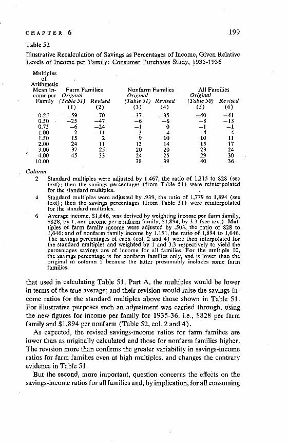
Table 52

Illustrative Recalculation of Savings as Percentages of Income, Given RelativeLevels of Income per Family: Consumer Purchases Study, 1935-1936

Multiplesof

ArithmeticMean In- Farm Families Nonfarm Families All Familiescome per Original Original OriginalFamily (Table 51) Revised (Table 51) Revised (Table 50) Revised

(1) (2) (3) (4) (5) (6)0.25 —59 —70 —37 —35 —40 —410.50 —25 —47 —6 —6 —8 —130.75 —6 —-24 —1 0 —1 —11.00 2 —11 3 4 4 41.50 15 2 9 10 10 112.00 24 11 13 14 15 173.00 37 25 20 20 23 244.00 45 33 24 25 29 30

10.00 38 39 40 36

Column2 Standard multiples were adjusted by 1.467, the ratio of 1,215 to 828 (see

text); then the savings percentages (from Table 51) were reinterpolatedfor the standard multiples.

4 Standard multiples were adjusted by .939, the ratio of 1,779 to 1,894 (seetext); then the savings percentages Table 51) were reinterpolatedfor the standard multiples.

6 Average incàme, $1,646, was derived by weighting income per farm family,$828, by 1, and income per nonfarm family, $1,894, by 3.3 (see text). Mul-tiples of farm family income were adjusted by .503, the ratio of 828 to1,646; and of nonfarm family income by 1.151, the ratio of 1,894 to 1,646.The savings percentages of each (col. 2 and 4) were then interpolated forthe standard multiples and weighted by 1 and 3.3 respectively to yield thepercentages savings are of income for all families. For the multiple 10,the savings percentage is for nonfarm families only, and is lower than theoriginal in column 5 because the latter presumably includes some farmfamilies.

that used in calculating Table 51, Part A, the multiples would be lowerin terms of the true average; and their revision would raise the savings-in-come ratiOs for the standard multiples above those shown in Table 51.For illustrative purposes such an adjustment was carried through, usingthe new figures for income per family for 1935-36, i.e., $828 per farmfamily and $1,894 per nonfarm (Table 52, col. 2 and 4).

As expected, the revised savings-income ratios for farm families arelower than as originally calculated and those for nonf arm families higher.The revision more than confirms the greater variability in savings-incomeratios for farm families even at high multiples, and changes the contraryevidence in Table 51.

But the second, more important, question concerns the effeèts on thesavings-income ratios for all families and, by implication, for all consuming

200 PART IIIunits in 193 5-36. The proper answer is contingent not only upon the revi-sion of the income for all farm and all nonf arm families but also upon thedistribution of revised totals by income brackets. An elaborate appor-tionment is unwarranted in view of the margin of error attaching to theresults. We made a simple adjustment, however, by weighting the mul-tiples for farm and nonfarm families (adjusted to take account of therevision in the average income of farm and nonfarm families) by 1 and3.3 respectively, representing roughly the relative weight of farm and non-farm families given in the 1935-36 study. In assigning the same weightsat each multiple position, we assume implicitly that the relative inequalityin income distribution is the same among farm and nonf arm families. Afterconverting each multiple underlying columns 2 and 4 to multiples 'for allfamilies, we interpolated again to get the savings-income ratios for farmand nonfarm families separately at the standard multiple levels. Weightingthese ratios by 1 and 3.3 respectively yielded the ratios for all familiesshown in column 6.

The revision alters materially the savings-income ratio at the multiple0.50 but not at the other multiples. It thus leaves the major conclusions inSection 3a intact. This may at first seem surprising but it is traceable tothe underlying figures: a decline in income per farm family from $1,232to $828, or about 33 percent, from 1929 to 1935-36; and a decline pernonfarm family from $2,932 to $1,894, or over 35 percent. Even moreimportant, farm families were estimated to number 5.8 million in 1929;nonfarm families, 21.7 miffion, or in the ratio of 1 to 3.7; the correspond-ing numbers for 1935-36 are 6.77 and 22.6 million respectively, or in theratio of 1 to 3.3. Thus, according to the two samples, from 1929 to1935-36 the income of farm families relative to that of nonfarm improvedslightly; moreover, farm families increased in number relative to nonf arm.Consequently, the bolstering effect of the much higher savings-incomeratios of farm families at the higher multiples was greater in 19.35-36 thanin 1929; and even though the ratios at the higher multiples for both farmand nonf arm families declined, the ratio for farm and nonfarm combinedbecomes almost constant or changes only slightly owing to the relativeimprovement in income and the relatively greater growth in the numberof farm families.

This conclusion is important in two respects. First, it partly explains thestability of savings-income ratios at upper income multiples in Section 3a:as far as such stability is attributable to the absence of a substantial declinein the ratios in 1935-36 it is due, if we use unrevised data for 1935-36, tothe possible overestimate of income per farm family, and if we use reviseddata, to a combination of shifts in income levels and weights between the

CHAPTER 6 201

farm and nonfarm family groups that may be unusual. In any event, wemust consider further to what extent the relative weight and levels offarm and nonf arm groups, or of any groups characterized by differentsavings-income ratios, accompany short term shifts in income associatedwith business cycles.

The second respect is perhaps more important. Total population, corn-prismg groups whose savings patterns differ materially, can have stablesavings-income ratios though the ratios of the groups change, and changein the same direction. In other words, the ratio for the total population isa complex of components whose savings responses to changing conditionsdiffer, and whose weights in the total income structure, as gauged by theirincome per unit levels and relative number of units, may shift concurrently.In a sense, therefore, a full explanation of .the stability or variability ofsavings-income ratios for groups at any income level is impossible withouta thorough account of the components. The explanations attempted beloware presented with cognizance of this limitation, and merely as preliminaryhypotheses designed to open the fieixl for more realistic analysis.

c) Brookings Special Sample for 1928-32In connection with its study of income and econàmic progress, the Brook-ings Institution distributed in 1933 a questionnaire designed to obtaininformation on savings by families with incomes above $5,000 (thoughsome recorded smaller incomes). Respondents were asked to report in-come including capital gains, expenditures, and savings for each year,1928-32. Of the 1,500-1,600 questionnaires tabulated, somewhat overa quarter were from university professors and teachers outside universities,about three-tenths from professional and managerial groups, about a thirdfrom federal employees and persons in clerical-mechanical occupations,and only about a fourteenth from business plus a special group with highincomes (either business or managerial, with a sprinkling of professional).Through the courtesy of Clark Warburton, we were given access to un-published tables summarizing this special sample which were preparedunder his direction and for his use; the original questionnaires were notavailable.

The sample material is presented in some detail in Appendix 1, Tables60-62 (see also America's Capacity to Consume, Brookings Institution,1934, App. B, pp. 254-5). Income per sample unit declines much less from1928-29 to 1932, somewhat over 20 percent, than countrywide incomeper unit, almost 50 percent. The chief reason for this relative stability isthe fact that the data were collected in 1933 from persons who were thenin occupations such as would be expected to yield incomes of $5,000 ormore. Obviously, persons in the same occupations or of similar economic

202 PART IIIstatus in 1928 who had lost their jobs, or who had had serious misfortunesbecause of the depression, were automatically excluded. For the samereason the over-all savings-income ratio for the sample declines much lessthan that for the country. Finally, because the sample was confined topersons expected to have incomes of $5,000 or more, the average level ofincome per unit is way above that for the country — from over twice toalmost four times as high (Table 61). In short, the sample is distinctlyoverweighted in favor of the higher income brackets and the more stabletypes of occupation.

For our purposes the sample has three other limitations: (a) capitalgains are included, and we must adjust for losses, which are given sep-arately in the summary tables; (b) the income information is by spendingunits, and we do not know their size (except in a few special high incomecases); (c) the data are subject to the errors that are common to informa-tion collected by a mail questionnaire. Yet it seemed worth while toanalyze the sample and observe what light it sheds on the movement ofsavings-income ratios at various income levels.

The summary tabulations classify the units first by their income for thegiven year (Table 60); then, those units that reported for each of the fiveyears, are classified by their average income for the quinquennium (Table62). The moderate reduction in the savings-income ratio for the sampleas a whole — from 29.6 percent in 1928 to 24.0 in 1932 (Table 60) andfrom 28.4 to 23.7 percent (Table 62) — might be taken as further supportof the relative stability of savings-income ratios at upper income levels(Sec. 3 a and b). But this inference is severely limited by the occupationalstructure of the sample: it obviously is not an unbiased sample of upperincome groups. Furthermore, as Table 61 shows, the income multipleposition of the sample as a whole rises steadily from 1928 to 1932, so thatfor a constant income multiple position, the savings-income ratio mightdecline more than that for the entire sample. We must, therefore, studythe data for the various income classes.

We first analyze the sample as classified by current year income, treatingit as we did the other samples — expressing the per unit of eachincome class as a multiple of countrywide income per unit, then inter-polating the savings-income ratios for such standard multiples as arewithin the range of the sample (Table 53, Part A). The one importantdifference is that here both the sample and the countrywide income includecapital gains and losses.

The upper multiples, say, 4.0 and 10.0, are probably the only onessignificantly affected by the inclusion of capital gains and losses: even inthe depression years, reported losses do not greatly affect the lower income

CHAPTER 6 203

Table 53

Summary of Analysis of Brookings Special Sample, 1928-1932

.A SAVINGS AS PERCENTAGES OF INCOME, GIVEN RELATIVE LEVELS OF INCOME PERUNIT

SAMPLE CLASSIFIED BY CURRENT YEAR INCOMEMultiples ofArithmetic

Mean Incomeper Unit 1928 1929 1930 1931 1932

0.50 0.9 —1.6 —18.8 —9.7 —17.20.75 14.7 13.0 4.2 2.3 —9.51.00 16.7 16.5 14.0 14.2 —1.71.50 21.6 19.9 19.1 16.3 10.82.00 23.8 22.? 21.8 21.1 17.03.00 25.3 28.0 24.6 23.1 22.14.00 31.1 32.2 24.4 24.2 22.3

10.00 39.7 38.3 34.5 34.1 31.3

B PROPORTION OF ABSOLUTE CHANGE IN SAVINGS PERCENTAGE TO PERCENTAGECHANGE IN INCOME (LIMITED TO INCOME CHANGE OF 5% OR MORE)

SAMPLE CLASSIFIED BY AVERAGE INCOME FOR 1928-32Change from1928, 1929, or

Income Classes Year to Year Change 1930 to 1932(ranked upward) Number A v. Proportion A v. Proportion

I 1 0.56 0.501! 1 0.24 0.53

III 1 * 0.21IV 1 0.15 0.23V 1 0.36 *

VI 1 0.09VII 1 0.11 *

VIII 1 0.09 0.09IX 1 0.02 *

X 1 0.10 0.19XI 2 0.44 0.27

XII 3 0.30 0.34XIII 2 0.13 0.11XIV 3 0.20 0,31

* Sign of change in income differs from that of change in savings percentage.

PART AArithmetic interpolation between multiples for the income groups in Table 61.

PARTBCalculated from Table 62 by the procedure described in the text. For income classescovered, see Table 60.

brackets (see Tables 60 and 62). The movement of the savings-incomeratios at income multiples below 4.0 confirms our conclusion that theratios at lower income multiples fluctuate more widely than those at thehigher multiples. For example, at the multiples 0.50, 0.75, and 1.0 therange is 20, 24, and 18 percentage points respectively; at the multiples 2.0and 3.0, it is 7 and 6 percentage points respectively.

204 PART IIIThe variations in the ratio become again somewhat wider for the mul-

tiples 4.0 and 10.0: 10 and 8 percentage points respectively. Even so,they are narrower in range than the variations for the multiples 1.0 andlower. Furthermore, the exclusion of capital gains and losses wouldpresumably reduce the savings-income ratios in the prosperous years, 1928and 1929, and increase them in the depression years, 1930-32. It wouldaffect also the multiple positions in the successive years and hence themovement of the savings-income ratios. Its effect on the latter cannot beestimated but is unlikely to be marked. Part A of Table 53 can be takenas confirming, on the whole, the stability of savings-income ratios at upperincome levels and their variability at lower levels.

Part J3 summarizes the results of our attempt to analyze the Brookingsspecial sample as a body of identical returns classified by their averageincome position for 1928-3 2. Here we are not interested in converting tomultiples in terms of current year countrywide income since the resultswould be roughly the same as those in Part A.12 Instead, for each of the 14income classes we found the changes from year to year and from 1928,1929, or 1930 to 1932 that represented an increase or decline of 5 percentor more in per unit income (smaller changes were ignored since their effecton the savings-income ratios was not likely to be significant). For eachpercentage change in income per unit we measured the absolute changein the savings-income ratio. In all except four cases the association waspositive — when income increased, the ratio rose; when income decreased,it fell.13 But our interest was mainly in the relation of the change in theratio associated with a percentage change in income at different levels.We therefore calculated for each change the proportion of the absolutechange in the ratio to the percentage change in income; and for incomelevels for which more than one such proportion was found, took a geo-metric mean of the proportions.

Since there wer'e few instances in which the percentage change in incomewas sizeable the results are somewhat limited in significance. However, inthe very low income classes, I and H, the proportions are fairly high; theytend to be quite low in the intermediate classes; and rise in the upperclasses, although they never reach the level of the proportions in Class I incolumns 2 and 3, or that in Class II in column 3.

It is clear that at the lower income levels a given percentage change in

12 Of the 1,587 questionnaires, only 59 did not cover all the years.Of the 20 significant year to year changes in income, only 3 were positive; and of

the 13 changes from 1928, 1929, or 1930 to 1932, only 1 was positive. The sampleis, therefore, preponderantly one in which declines in income cause declines insavings-income ratios.

CHAPTER 6 205

income is associated with a much larger absolute change in the savings-income ratio than is the same or a similar percentage change in income atthe intermediate or upper levels; and there is some evidence that savings-income ratios at the upper income levels are more sensitive to percentagechanges in income than those at the intermediate; but how much is due tothe effect of including capital gains and losses can be only conjectured.Part B of Table 53 thus more or less confirms Part A, though only as tothe variability of the savings-income ratios at very low income levels.

Finally, the savings-income ratios at upper levels are more variablewhen the levels are based on average income for a longer period than whenbased on current year income. In the classification by average income wedeal with a continuous identical• body of units in the upper and lowerbrackets, which removes the effects of mobility. Mobility may well have amore stabilizing (or less disturbing) effect on the savings-income ratios ofupper than of lower income groups (Sec. 4), and may explain why savings-income ratios at upper levels appear more stable in Part A than in B. How-ever, the difference is too small to be considered of much importance.

4 Factors Making for Stability of Savings-Income Ratios at Upper IncomeLevels

The empirical analysis in Section 3, bearing upon the relative variability ofsavings-income ratios at upper and lower income levels, is subject tonumerous qualifications. We mention the most important before attempt-ing to indicate the factors that may explain them.

First, the sample data yield general levels of savings-income ratios thatare far higher than those obtained by other methods used by the authorand recently by the Department of Commerce which involve comparisonsof income and expenditures. True, deriving savings by such comparisonsmay causô large errors. Yet even allowing for such lack of reliability inyear to year estimates, it is a matter of concern that the average savings-income ratios from the sample studies are almost uniformly so much higherthan those derived by the residual method. Some of the difference may bedue to the inclusion of certain depreciation and expense items (e.g., de-preciation on owner-occupied houses, and brokers' fees) in the sampleestimates of savings; some to an underestimate of expenditures comparedwith income. On the other hand, the shortages in estimates of countrywideincome may be larger than those in consumer expenditures, and the resid-ual method may well yield a smaller total for savings, and hence a lowerlevel of the savings-income ratio than the true one.

Since the first qualification affects only the average level of savings-in-come ratios it is not likely to affect the analysis of their short term changes.

206 PART IIIThe second qualification is more important: the sample data are confinedlargely to cyclical expansions, and shed little light on movements of sav-ings-income ratios during contractions. Yet the Brookings special samplecovering the 1930-32 depression suggests the same conclusion; and f orthe years covered by the different samples, the over-all ratio varies con-siderably. In the sample data (Assumption 2 for 1929), savings con-stituted 17 percent of income in 1929, 10 in 1935-36, 9 in 1941, 12 in1942, 15 in 1945, 12 in 1946,9 in 1947, 7 in 1948, 5 in 1949, and 8 in1950. The unadjusted savings-income ratios thus ranged from 5 percentto over three times that; and it is against this background that the relativestability of savings-income ratios at upper income levels must be con-sidered.

The third qualification lies in the errors that can be attributed to thesample data, particularly the few cases covered at the upper income levels.Few samples reach the upper tail of the size distribution; most stop belowthe income multiple levels associated with the top 5 percent group in ouranalysis in Chapters 1-5. And a special case of uncertainty created by thecharacter of the sample is the difficulty of choosing between Assumptions1 and 2 in our treatment of the 1929 data.

Yet all these qualifications do not undermine the main conclusion fromthe sample data: the smaller relative variability of savings-income ratiosat upper than at lower income levels. Furthermore, they strongly suggestsmaller absolute variability at upper levels, say, top 5 to 10 percent.

Dorothy Brady and Rose Friedman came to a similar conclusion con-cerning absolute variability, though for urban families alone, in Savingsand the Income Distribution, Studies in Income and Wealth, Volume Ten(p. 261). Their Chart 4 shows the savings are of income forurban families classified by the ratio of their income to average income,i.e., by our multiples. For the multiple 2.0 the ratios in 1917-19, 1935-36,and 1941 are almost identical; and in 1935-36 and 1941 the ratios forthe multiples from 2.0 to above 3.0 are very similar; they diverge muchmore at multiples below 2.0. However, the ratios for their 1901 sampleare much higher at multiple 2.0 and above. Evidently stability of savings-income ratios at high income levels characterized the 1920's and 1930'sbut not the beginning of the century. Still, as far as one can tell, the averageincome levels in the successive years have not been tested for cçmparabil-ity,Le., Chart 4 is based on unadjusted multiples and adjustments mightmodify the results.

The importance of the narrower absolute variability of savings-incomeratios at upper than at lower income levels, and the qualifications thatnecessarily attach to the empirical analysis in Section 3, warrant some

CHAPTER 6 207

further exploration. We therefore consider the factors that might makefor greater absolute stability ,of savings-income ratios at upper incomelevels.a) The first factor is purely technical. It can be presented in a simple illus-tration, then generalized in an equally simple mathematical expression.Assume that in a given year real income is 400, that each of four incomeclasses has a total' income of 100, and that the savings-income ratios forthese classes are 40, 20, 0, and —20 percent respectively. These incomeclasses with vastly different income levels per capita would spend 60, 80,100, and 120 percent respectively 'of their base-year income. Assume thatreal income rises percent, so that total income the next year is 480;and that each income class continues to spend exactly what it spent thepreceding year. What happens to their savings-income ratios providedtheir real incomes also rise 20 percent, i.e., that their relative shares intotal income remain the same?

In the top class income increases from 100 to 120, and since expendi-tures remain the same, savings increase from 40 to 60. The savings-incomeratio rises from 40 to 50 percent (60/120). The income of the secondclass increases from 100 to 120, expenditures remain at 80, savings in-crease from 20 to 40, and the savings-income ratio rises from 20 to 33percent (40/120). The income of the third class increases from 100 to120, expenditures remain at 100, savings increase from 0 to 20, and thesavings-income ratio rises from 0 to 17 percent (20/120). Finally, in thebottom class income increases from 100 to 120, expenditures remain at120, savings increase from —20 to 0, and the savings-income ratio rises

,from —20 to 0 percent. The point of the illustration is that with an equalrelative increase in income and stable expenditures the savings-incomeratio rises 10 percentage points in the top income class, 13 in the second,17 in the third, and 20 in the bottom.

The results would be similar, in fact somewhat accentuated, if weassumed a 20 percent decline in real income while retaining all the otherassumptions: the savings-income ratios would decline least in the topincome class and most in the bottom. Likewise, if instead of assuminginflexible expenditures in real terms, i.e., complete lack of response tochanges in real income, we assumed partial response, so that at eachincome level consumption would rise or decline but relatively less thanincome, the absolute change in the savings-income ratio would still be leastin the top income class and most i.n the bottom.

This conclusion can be generalized by introducing four equations. Leti be income; e expenditures; s savings; k proportional change in income;ak proportional change in expenditures, a ranging from 0 to 1; R the

208 PART IIIsavings-income ratio. A plus sign as subscript indicates the item in the yearfollowing the base year. Then:

R— i(1+k)—e(1+ak) — i+ik—e—ake

2i(1+k) — i(1+k)i+ik—e—ake i—e

i(1+k) — i

ek—ake — ek(1—a)(3)i(1+k) — i(1 +k)

But from (1): e = i (1 — R). Hence, we get in

R —R—-i(1—R)k(1—a) — k(l_a)(lR) (4)

+ i(1+k) — 1+kIf k and a are the same at all income levels, it follows that:

(i) As R grows progressively smaller from the upper to the lower brackets,

the absolute change in the savings-income ratio (R+ — R) grows larger.(ii) Given the value of k, the change in the savings-income ratio will besmaller the larger a is and vice versa; it will be at a maximum when a 0.

(iii) Given the value of a, the change in the savings-income ratio will varywith the value of k, but k/(1 + k) will be weighted for each incomebracket by the factor (1 — a) (1 — R).

If a is less than 1 and is identical from income bracket to income bracket,the same proportional change in income will produce a smaller absolutechange in the savings-income ratios at upper than at lower brackets. Bydefinition, equal multiples of average income in two or more years repre-sent a percentage change in income equal to the percentage change in totalincome. Hence k by definition is equal at the same multiples. What remainsto be explored is whether a tends, in the short run, to differ between thehigh and low income multiples; and whether such differences reenforce oroffset the conclusions from equation (4) •14

Our analysis can be restated in terms of average and marginal propensity to save(spend). R and R+ are the average propensities to save, i.e., s/i and s÷/i+, where s and

i are savings and income for the respective years. Marginal propensity to save (andspend.) is defined as (and where is the change in savings, d6 thechange in expenditures, and the change in income.

a in the text equation is the relative marginal propensity to spend and equals(d,/R); = • (i/R). The absolute marginal propensity to save(spend) equals the product of the relative marginal propensity and the savings-(spendings-) income ratio in the initial year of the period.

CHAPTER 6 209

b) The general hypothesis here is that a, i.e., the ratio of the relativechange in expenditures to that in total income, is likely to vary more atupper multiples than at lower. In other words, the expenditures of upperincome classes are more sensitive to fluctuations in income than those oflower, making for short term stability of the savings-income ratios at upperbrackets and short term variability at lower.

This hypothesis is most plausible if we first deal with a period duringwhich real income declines. Expenditures at lower income levels can becurtailed only with difficulty for the simple reason that most consumergoods purchased are in the nature of necessities and contraction encountersserious, almost physiological, obstacles. Since expenditures of consumersat low income levels are chiefly on food, shelter, and clothing, a sizeablereduction may be inimical to health. Expenditures at upper income levels,on the contrary, are much more heavily weighted by luxuries and semi-

The conclusions from equation (4) can, therefore, be expressed as follows. If theaverage propensity to save changes during the period because the marginal propen-sity differs from the average in the initial year, the change is inversely related to thelevel of the average propensity to save in the initial year provided the relative mar-ginal propensity to spend is the same for all income classes.

Equation (4) parallels those of Franco Modigliani (Studies in income and Wealth,Volume Eleven, NBER, 1949) and James Duesenberry (income, Employment andPublic Policy, Essays in Honor of Alvin H. Hansen, Norton, 1948, pp. 54-82). Bothauthors express the over-all savings-income ratio by an equation in which there isa constant term and a term moving with the ratio of the given year income to thepreceding cyclical peak income. When R is defined as the savings-income ratioduring the preceding cyclical peak year, and a, the proportion associated with thelatter, both become constants; and R. may be defined as the savings-income ratiofor any subsequent year. On this interpretation, k becomes the proportional changein income from the preceding cyclical peak income; and equation (4) can be rewrit-tenas R •R k1_R_1+R+(l_a)1+kSince R and a are constants, the changing R+ is a function of a constant term

(iR) and a term moving with k, the ratio of the given year income to the pre-

ceding cyclical peak income.However, we need not define R and a as ratios associated with the preceding

cyclical peak or k as relating to changes in income from the preceding cyclical peak.They may well refer to the preceding year or to secular levels (of theratio or the propensity to consume). The role to be assigned to R, a, and k remainsto be explored in the light of what yields the most efficient account of empiricallyobserved short term changes in R+. What is particularly important here is that aneed not be the same for all income groups; and the short term variations in R+,the latter conceived as the over-all savings-income ratio, are much more complexthan Modigliani and Duesenberry assume.

210 PART IIIluxuries, and contraction, while still painful because of the desire to main-tain class standards, is easier. One can, therefore, infer that when realincome per capita declines, expenditures will be curtailed proportionatelyless at lower than at upper income levels; in other words, that a will behigher at lower levels. Clearly, this difference in the response of expendi-tures to contraction will be wider the larger the relative contraction in realincome per capita. If the decline is just 1 or 2 percent, a may well be thesame through the range of income multiples; if the decline is 20 percent,the difference in the response of expenditures at the various income levelsis likely to be much wider.

If this relative inflexibility of expenditures at lower income levels andgreater flexibility at upper levels is accepted as characterizing short termdeclines in per capita income, consequences follow for short term increases.Offhand, one would surmise that when per capita income increases,expenditures would tend to increase proportionately more among lowerincome groups than among upper: the former live closer to the margin ofsubsistence and have a much bigger unsatisfied potential. But in the con-tinuous succession of short term cyclical changes increases in real incomesucceed decreases. During declines the lower income groups tend to dis-save, either reducing their savings reserves, always relatively inadequate,to dangerously low levels or piling up a large net indebtedness. Hence,when recovery comes and income increases, any tendency to spend moreis checked by the need to repay debts and by the desire to rebuild a safereserve. Thus, the relative inelasticity of expenditures at low income levelsduring short term declines in income carries over into periods of increasesin income, damping the responsiveness of current expenditures to a currentincrease in real income.'5

If income per capita continues to increase for some time the effects of the precedingcontraction are likely to diminish, perhaps vanish. At the end or in the later phasesof a long cyclical expansion accompanied by a substantial increase in real incomeper capita, expenditures at the lower incomes multiples may become fully respon-sive to an increase in income, giving a a value not much lower than at the uppermultiples.

Another complicating factor is the effect of consumer credit. If consumer creditis of major importance in budgets at the lower multiples, the net addition to itduring cyclical expansions enhances the responsiveness of expenditures to increasesin income; likewise, the net contraction of consumer credit during cyclical declinesenhances the sensitivity of expenditures to declines in income. However, it may wellbe that consumer credit is more important at the intermediate than at the very lowincome levels. If so, its cyclical responsiveness would tend to make the a values forthe intermediate income groups higher than for the low groups, and bring themcloser to those for the upper groups to whom consumer credit may be of littlemoment.

CHAPTER 6 211

Another reason for the greater sensitivity of expenditures at upperincome levels is that holdings of assets are heavily concentrated there, andfluctuations in their value, even if not realizedin the form of capital gainsor losses, are keenly felt. Increases in their value during cyclical expan-sions, i.e., during short term increases in real income per capita, are likelyto induce upper income groups to spend more. The impression of largerinvestment reserves and optimism concerning their adequacy in the futuretakes on the opposite hue during cyclical contractions, when the value ofassets declines. Thus in expansions, upper income groups may spend morethan they would were they not misled by the illusion of the rising valueof assets; and in contractions, they may cut expenditures more than theywould if declining property values did not cause them to worry about thefuture. These illusions affect the lower income groups too, but less, sincea larger proportion of their incomes are wages and salaries, which do notfluctuate as violently as do assets. They operate regardless whether gainsand losses are realized by sales of assets.c) The discussion so far has dealt with income groups as if their compo-sition remained the same, i.e., we have disregarded inter-class movementsof the type studied in Chapter 4. During short periods such movementsare limited and a given income class contains a large proportion of thesame units in successive years. But some shifts do occur, and their effectson the behavior of savings-income ratios for upper and for lower incomegroups must be explored. Lack of data makes the exploration largely amatter of conjecture.

In this hypothetical analysis we must consider not merely income mul-tiples, i.e., points on the income scale, but classes, since only for the lattercan groups of units be observed and movements studied. We deal thenwith income classes as represented by income multiples, and distinguishbetween an income unit whose real income does not change during a giveninterval (designated R for 'resident'), and one whose real income rises ordeclines (a 'migrant up' is designated Mu, a 'migrant down', Md). Thedistinction between an R and an M is the constancy or change in its amountof income, not its income rank.

The systematic changes during business cycles can easily be postulated.During expansions and contractions there are R's, Mu's, and Md's, butthere are more M's when levels of activity change materially; and Mu'soutnumber Md's during expansions, whereas the reverse is true duringcontractions. In this continual movement of Md's and Mu's do the effectsupon the savings-income ratios for upper and for lower income groupsdiffer?

In an income group characterized by a given income multiple there are

212 PART IIIR's, Mu's, and Md's. At a given income level the Mu's are likely to havea higher, and the Md's a lower, savings-income ratio than the R's. Thespread between the ratios of R's and M's will depend upon the relativelevel of income. But for the present we may ignore this point.

The first obvious difference is that between extreme and intermediateincome classes. In the lowest income class, classified by current income,there can be R's and Md's but few Mu's; in the intermediate classes therecan be both Mu's and Md's, with an income balance of the two morepossible the nearer the class is to the center of the distribution; and in thevery top class there can be R's and Mu's but few Md's. On the averageand disregarding short term fluctuations, the extreme income classes andthose near them will have a preponderance of either Md's or Mu's; hencetheir savings-income ratios are likely to be lowered and raised more byinter-class migration, i.e., by the effect of the M's.

These statements, bearing upon the average effects of migration on thesavings-income ratios for the extreme and intermediate income classesrespectively, explain why, on the average, the ratios for the extreme incomeclasses are so conspicuously low or high compared with those for theintermediate classes. In thinking of what this means in terms of temporalchange, one is likely to conclude that during short term cyclical changes,variations in the income displacement attributable to the Mu's andMd's are likely to be larger for the extreme income classes than for theintermediate.16

But whether income displacement is greater or less for upper than forlower income groups, its effect on savings-income ratios is likely to beless at the upper levels. As noted in Section 3, the function associatingsavings-income ratios with income multiples looks like an hyperbola, ris-ing rapidly (almost vertically) in the change from the very low multiplesto the intermediate ones and flattening out as we reach the high multiples.And since beyond the multiple 5.0 or so, the savings-income ratios barelyrise, a similar shape would be preserved were we to use logarithms ofmultiples on the X scale — in the sense that the curve would still flattenbeyond a certain high multiple level. Hence, when an income unit moves

10 This conjecture, as far as it refers to absolute income displacement, is not con-firmed by the Wisconsin sample of identical returns for 1929-35. But this sampledoes show that displacement measured relatively to the income level of a given classdeclines in amplitude as we pass from the lower to the upper income brackets —another factor accounting for the stability of savings-income ratios at upper levels.In view of the limited value of the Wisconsin data, which do not reach far downthe income distribution, it did not seem worth while to present the results or toattribute much significance to them.

CHAPTER 6 213

into a higher or lower class within the income range well below the top, agiven change in its income causes a large change in the savings-incomeratio; when a similar movement occurs at the high income levels, a givenchange, whether absolute or relative, in its income does not greatly affectthe ratio. True, the function just described is derived for income classesaffected by migration, and hence may be due partly to differences in therelative income displacement associated with income level. But it maybe surmised that could we study resident units alone, the slope of the lowand the high segments of the income distribution would still differ. Thismeans that, in addition to differences between the low and high incomeclasses in the amplitude of short term changes in relative income migration,differences in the impact of income displacement also minimize the shortterm changes in the savings-income ratios for upper groups.

Finally, shifts associated with specific types of income may producedifferentials in short term changes in savings-income ratios at differentpoints on the income scale. As observed in Section 3b, the spread of thesavings-income ratios for farm families was wider than for nonf arm fami-lies for the same range of income multiples; and at the higher multiples,where savings were positive, the ratios were consistently and appreciablyhigher for farm families. The factors explaining these differences betweenfarm and nonfarm families may apply, in large part; also to a comparisonbetween units depending upon entrepreneurial income and those depend-ing mainly upon other, cyclically more stable, types of income.

The per unit income of entrepreneurial groups, whether farm or non-farm, may rise during cyclical expansions and decline during contractionsmore than the per unit income of other groups. But for these entrepre-neurial groups savings-income ratios may be higher at the same levels ofincome, once we pass the minimum level that yields positive savings; andthe relative weight of entrepreneurs, particularly farm entrepreneurs, inthe population, may increase during substantial cyclical contractions anddiminish during substantial expansions. The latter shift may raise savings-income ratios at upper income levels during contractions and depress themduring expansions although the ratios of the entrepreneurial groupsproper, and of other groups, decline during contractions and rise duringexpansions. Elements of stability would thereby be introduced into theratios at such multiples as can be influenced by the relative number andsavings patterns of the entrepreneurial groups. This would presumablynot affect the very top income brackets, where incomes of entrepreneurs,especially of farm and similar small scale individual business men, play aminor role. Yet it may affect the savings-income ratios at the multiplesfrom, say, 2.0 to 4.0, as in the analysis in Sections 3a and b.

214 PART III5 Summary and ImplicationsAs far as upper income groups can be characterized by their averageincome levels, they are at high multiples; consequently if their relativeincome position were constant during business cycles, their savings-incomeratios would fluctuate with a much narrower relative amplitude than thoseof lower groups. Furthermore, the greater relative stability of their sav-ings-income ratios is reenforced by the counter movement of their incomemultiple position to business activity, except for the irregular behavior ofthe share of the top 1 percent. The movement in the ratios for upperincome groups is a product of two sets of opposite changes: the counter-cyclical movement of their income shares (multiple positions) and themovement of the ratios at given upper income multiples with businesscycles. We cannot tell with any assurance what the net effect of theseopposite movements is in setting the cyclical pattern of changes in thesavings-income ratios of upper groups: in most pronounced cyclical shiftsthe positive pattern of the ratios for a given multiple position probablyoutweighs the inverted pattern of shifts in income shares, i.e., in incomemultiple position, making the ratios for upper groups move with businesscycles.

Even so, the savings of upper income groups must vary less cyclicallythan those of lower groups — for two reasons: (a) the inverted movementof upper group shares in total income tends to offset the positively con-forming movement of savings-income ratios for given income multiples,whereas for lower income groups both the shares of total income receivedand the ratios move with business cycles; (b) the savings-income ratiosvary less for upper multiples than for lower, and the difference in the rela-tive variation must be quite large.'7

As far as the savings of upper income groups, expressed as percentages

Of all the evidence examined so far oniy one item for recent years qualifies thegeneralization that savings-income ratios for upper income groups change less abso-lutely than those for lower groups (both groups taken widely). George Katona ofthe University of Michigan Survey Research Center kindly provided a break at theupper S percent line for the samples for 1946-48 (Surveys of Consumer Finances).The ratio for the top 5 percent group declined from 26 percent in 1946 to 21 percentin 1947 and to 17 percent in 1948, 9 points. The corresponding ratio for the lower95 percent declined from 8 percent in 1946 to S in 1947 and to 4 in 1948, only 4points. We do not know how far this larger absolute, but not relative, decline in theratio for the top group depends upon the exceptional conditions in 1946-48 or uponpeculiarities of the sample. However, the sample data still support our basic conclu-sion that when the over-all savings-income ratio declines, the share of upper groupsin savings increases. Thus while the over-all ratio in the sample declined from about12 to about 7 percent, the share of the top 5 percent group .in total savings increasedfrom SO to 58 percent.

CHAPTER 6 215

of individuals' total income receipts, are stable or vary little, whereas thesavings of lower groups vary markedly with business cycles, two furtherconclusions follow. First, the marked fluctuations in the over-all savings-income for individuals and its conformity to business activity mustbe due largely to variations in the ratios for lower income groups; they canbe attributed only in small part to variations in either the income shares orthe ratios for upper groups. Second, the shares of upper and lower incomegroups in individuals' total savings must change significantly during busi-ness cycles: as total savings and their ratio to total income rise duringexpansions, the percentage shares of upper groups must decrease; as totalsavings and their ratio to income decline during contractions, they mustincrease. In years of cyclically high savings by individuals, upper incomegroups must contribute proportionately less, and in years of low savings,more; lower income groups must do the opposite.

These conclusions are subject to several qualifications. The sampledata we had to use were scanty, particularly in their coverage of the topincome group and of cyclical contractions; and our adjustments wereunavoidably crude. Furthermore, our analysis covers a period so short thatwe can merely surmise, not generalize. Yet one aspect of our conclusionsis worthy of emphasis. If the average level of the savings-income ratio forupper groups (say, top 5 or 10 percent) is 25 or 30 percent, and that forlower groups 5 percent or less, the relative variability of the former canhardly be as wide as that of the latter. Consequently, the greater relativevariability of savings-income ratios for the latter is so highly probable as tobe almost in the nature of an algebraic necessity. If this is granted, theinference concerning the counter-cyclical movement of upper group sharesin total savings must follow.

By way of final illustration we present Table 54, which in a sense restatesdata used in Section 3, but brings out more distinctly the associationbetween changes in the over-all savings-income ratio and in the share ofindividuals' total savings accounted for by upper income groups. For thetwo samples that cover more than a year and for which savings-income ratios and in the shares of both income and savings can thereforebe studied without adjustment for comparability, we assembled measuresof over-all savings-income ratios and of shares of the upper one-tenth andlower nine-tenths savings and income. All these were taken from thesample distributions, with only minor adjustments. The groups are classi-fied by income per consuming or spending unit.

Whenever the over-all savings-income ratio rises from one year to thenext, the percentage share of upper income groups in individuals' totalsavings declines; and whenever it declines, their share rises. The consistent

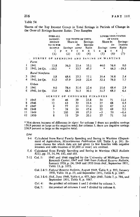
216 PART IIITable 54

Shares of the Top Income Group in Total Savings in Periods of Change inthe Over-all Savings-Income Ratio: Two Samples

OVER-ALL LOWER NINE-TENTHSSAVINGS- TOP TENTH OF UNITS OF UNITSINCOME Share in Savings- Share in Savings-

RATIO FOR in- Income in- IncomeSAMPLE Savings come Ratio Savings come Ratio

( p e r c e n t a g e s )(1) (2) (3) (4) (5) (6) (7)

SURVEY OF SPENDING AND SAVING IN WARTIMEFarm

1 1941 13.8 56.0 23.4 33.1 44.0 76.6 8.02 1942, 1st Qu. —10.2 * 33•7 47•3 * 66.3 39.3

Rural Non/arm3 1941 5.8 68.6 23.2 17.1 31.4 76.8 2.44 1942, lstQu. 11.2 47.9 24.0 22.4 52.1 76.0 7.7

Urban5 1941 9.0 78.4 31.6 22.4 21.6 68.4 2.96 1942, lstQu. 13.9 68.3 31.5 30.1 31.7 68.5 6.4

SURVEY OF CONSUMER FINANCES -

7 1945 15 46 29 23.8 54 71 11.48 1946 12 63 32 23.6 37 68 6.59 1947 9 77 33 21.0 23 67 3.1

10 1948 7 78 31 17.6 22 69 2.211 1949 5 105 30 17.5 —5 . 70 —0.412 1950 8 73 29 20.1 27 71 3.0

* Not shown because of difference in signs: for column 2 there are positive savings156.9 percent as large as the negative total; for column 5, there are negative savings256.9 percent as large as the negative total.

Line1-4 Calculated from Rural Family Spending and Saving in Wartime (Depart-

ment of Agriculture, Miscellaneous Publication 520, Table 5, P. 26). In-come classes for which data are not given (a few families with negativeincomes and with incomes of $5,000 or over) are omitted.

5, 6 Calculated from Family Spending and Saving in Wartime (BLS Bulletin822), pp. 33, 34, 94, 102, and 103.

7-12 Col. 1: 1945 and 1946 supplied by the University of Michigan SurveyResearch Center; 1947 and 1948 from Federal Reserve Bulletin,January 1950, P. 24; 1949 and 1950 from ibid., September 1951,Table 13, p. 1072.

Col. 2 & 5: Federal Reserve Bulletin, August 1949, 'fable 9, p. 923, January1950, Table 10, p. 23, and September 1951, Table 8, p. 1067.

Col. 3 & 6: ibid., June 1948, Table 4, p. 653, July 1949, Table 7, p. 786, andSeptember 1951, Table 8, p. 1067.

Col. 4: the product of columns 1 and 2 divided by column 3.Cot. 7: the product of columns 1 and 5 divided by column 6.

CHAPTER 6 217

negative association between changes in the over-all ratio and in the pro-portion of total savings contributed by upper income groups is due to anegative association between changes in the income share of upper groupsand in the over-all ratio, and a consistently narrower relative, and oftenabsolute, change in the savings-income ratio of the upper than in that ofthe lower income groups.

The significance of Table 54 is limited by the smallness of the samplesand especially by the presence of war years in the period covered.theless, it is further evidence that short term variations in the percentageshares of upper income groups in individuals' total savings are large andrun counter to variations in the over-all savings-income ratio, hencecounter to business cycles.

Further implications of this conclusion cannot be pursued here. How-ever, they seem, at least at first glance, to be far reaching. The savings ofupper and of lower income groups tend to flow into different kinds ofinvestment. Upper groups dominate in receipts of dividends and dividendsconstitute a large proportion of their property incomes. Their savingsmay, therefore, flow into dividend-bearing assets to a much greater extentthan those of lower groups. Of the property incomes of lower groups, onthe contrary, dividends constitute a small proportion; and one would sur-mise that their savings go largely into interest-bearing assets or into equi-ties in small business units. Similar evidence concerning differences in thecomposition of assets held by upper and lower income groups is providedby the 1949 Survey of Consumer Finances (Federal Reserve Bulletin,Aug. and Sept. 1949). Cyclical shifts in upper group shares in total savingsmay alter the proportion of individuals' savings available for different typesof investment, and an analysis of the relation between the new supply ofsavings and of investment opportunities during business cycles must takeaccount of cyclical shifts in savings coming from upper and from lowerincome groups.

There are similar consequences in the distribution of consumptionexpenditures between those by upper and by lower income groups. Thecounter-cyclical movement of income shares and the lesser variability insavings-income ratios for upper groups mean that a .decreasing share ofincome in expansions is offset by only a moderate rise in the ratio, whereasfor the lower groups an increasing share of income may be offset by asharp rise in the ratio. The proportion of upper group expenditures in totalconsumer expenditures may rise during expansions, or at least through asubstantial part of them, and decline during contractions. But in the caseof consumer expenditures, the counter-cyclical movement of the incomeshares of upper groups makes for a similar movement in the proportion

218 PART IIIof upper group expenditures in total expenditures, whereas the movementof the savings-income ratio makes for cyclical conformity in that propor-tion. Thus, while the proportion of upper group savings moves counter tobusiness cycles because of both the counter movement of income sharesand the narrower amplitude of changes in the savings-income ratio, theproportion of upper group expenditures is subject to conflicting pressures— one, the movement of income shares, making for a counter-cycle pattern,the other, the narrower amplitude of changes in the savings-income ratio,making for a movement with business cycles. Because the effects may beoffsetting, and also because the average shares of the upper groups in totalexpenditures are much smaller than those in total savings, the cyclicalchanges in the former may be quite small; and it is not clear whether theywould run counter to or with business cycles.