SHARE Wave 5 · ISBN 978-3-00-049309-6 SHARE Wave 5: Innovations & Methodology This volume...
180
Edited by: Frederic Malter Axel Börsch-Supan SHARE Wave 5: Innovations & Methodology
Transcript of SHARE Wave 5 · ISBN 978-3-00-049309-6 SHARE Wave 5: Innovations & Methodology This volume...

ISBN 978-3-00-049309-6
SHA
RE W
ave
5: In
nova
tion
s &
Met
hodo
logy
This volume documents the most important questionnaire innovations, methodological advancements and new procedures introduced during the � fth wave of the Survey of Health, Ageing and Retirement in Europe (SHARE). SHARE’s main aim is to provide data on individuals as they age and their environment in order to analyse the pro-cess of individual and population ageing in depth. SHARE is a distributed European research infrastructure which provides data for social scientists, including demographers, economists, psychologists, sociologists, biologists, epidemiologists, public health and health policy experts who are interested in population aging.Covering the key areas of life, namely health, socio-economics and social networks, SHARE includes a great variety of information: health variables (e.g. self-reported health, health conditions, physical and cognitive functioning, health behavior, use of health care facilities), bio-markers (e.g. grip strength, body-mass index, peak � ow; and piloting dried blood spots, waist circumference, blood pressure), psychological variables (e.g. mental health, well-being, life satisfaction), economic variables (current work activity, job characteristics, opportunities to work past retirement age, sources and composition of current income, wealth and consumption, housing, education), and social support variables (e.g. assistance within families, transfers of income and assets, volunteer activities) as well as social network information (e.g. contacts, proximity, satisfaction with network). Researchers may download the SHARE data free of charge from the project’s website at www.share-project.org.SHARE combines multi-disciplinarity with being genuinely multi-national. In Wave 5, we collected interview data from about 85,000 individuals aged 50 or over from 19 countries. Moreover, SHARE is harmonized with the U.S. Health and Retirement Study (HRS) and the English Longitudinal Study of Ageing (ELSA). Studies in Korea, Japan, China, India, and Brazil follow these models. Rigorous procedural guidelines, electronic tools, and instruments are designed to ensure an ex-ante harmonized cross-national design.
Edited by:Frederic MalterAxel Börsch-Supan
SHARE Wave 5: Innovations & Methodology


SHARE Wave 5: Innovations & Methodology

4
SHARE Wave 5: Innovations & Methodology
Edited by:Frederic MalterAxel Börsch-Supan
Authors:
Mauricio AvendanoAxel Börsch-SupanJohanna BristleMartina Celidoni Enrica CrodaDominika DudaSabine FriedelChristian Hunkler Hendrik JürgesThorsten KneipJulie Korbmacher Ulrich KriegerAnne LaferrèreGiuseppe De Luca Frederic MalterMaurice MartensMichał Myck Monika Oczkowska Claudio RosettiGregor SandDaniel SchmidutzMorten SchuthElisabetta TrevisanMelanie WagnerIggy van der WielenArnaud Wijnant

5
Published by:Munich Center for the Economics of Ageing (MEA) at the Max Planck Institute for Social Law and Social Policy (MPISOC)Amalienstrasse 3380799 MünchenTel: +49-89-38602-0Fax: +49-621-38602-390www.mea.mpisoc.mpg.de
Layout and printing by:VALENTUM KOMMUNIKATION GMBHBischof-von-Henle-Str. 2b93051 Regensburg
© Munich Center for the Economics of Ageing, 2015
Suggested citation:
Malter, F. and A. Börsch-Supan (Eds.) (2015). SHARE Wave 5: Innovations & Methodology. Munich: MEA, Max Planck Institute for Social Law and Social Policy.
ISBN 978-3-00-049309-6

6
1 SHARE Wave 5: Balancing innovation and panel consistency 8
Axel Börsch-Supan and Frederic Malter, Munich Center for the Economics of Aging MEA at the Max Planck Institute for Social Law and Social Policy (MPISOC)
2 Questionnaire innovations in the fifth wave of SHARE 15
2.1 Questionnaire development in the fifth wave of SHARE 16 Frederic Malter, Munich Center for the Economics of Aging (MEA) at the Max Planck Institute for Social Law and Social Policy (MPISOC)
2.2 Measuring early childhood circumstances in SHARE Wave 5: 18 A “mini childhood” module Mauricio Avendano, London School of Economics and Political Science & Harvard School of Public Health Enrica Croda, Department of Economics, Ca’ Foscari University of Venice
2.3 Innovations for better understanding deprivation and social exclusion 29 Michał Myck, Monika Oczkowska and Dominika Duda, Centre for Economic Analysis (CenEA), Szczecin
2.4 Health care utilization and out-of-pocket expenses 37 Hendrik Jürges, University of Wuppertal
2.5 Identifying second-generation migrants and naturalized respondents in SHARE 43 Christian Hunkler, Thorsten Kneip, Gregor Sand and Morten Schuth, Munich Center for the Economics of Aging (MEA) at the Max Planck Institute for Social Law and Social Policy (MPISOC)
2.6 SHARE questionnaire encyclopaedia 48 (or “question-by-question manual” or “Q-by-Q”) Anne Laferrère, National Institute for Statistics and Economic Studies (INSEE), Paris Frederic Malter, Munich Center for the Economics of Aging (MEA) at the Max Planck Institute for Social Law and Social Policy (MPISOC)
3 Software innovations in SHARE Wave 5 51
Maurice Martens, Iggy van der Wielen, Arnaud Wijnant, CentERdata, Tilburg University Gregor Sand, Munich Center for the Economics of Aging (MEA) at the Max Planck Institute for Social Law and Social Policy (MPISOC)
CONTENTS

7
4 A note on record linkage in SHARE 60
Julie M. Korbmacher, Daniel Schmidutz, Munich Center for the Economics of Aging (MEA) at the Max Planck Institute for Social Law and Social Policy (MPISOC)
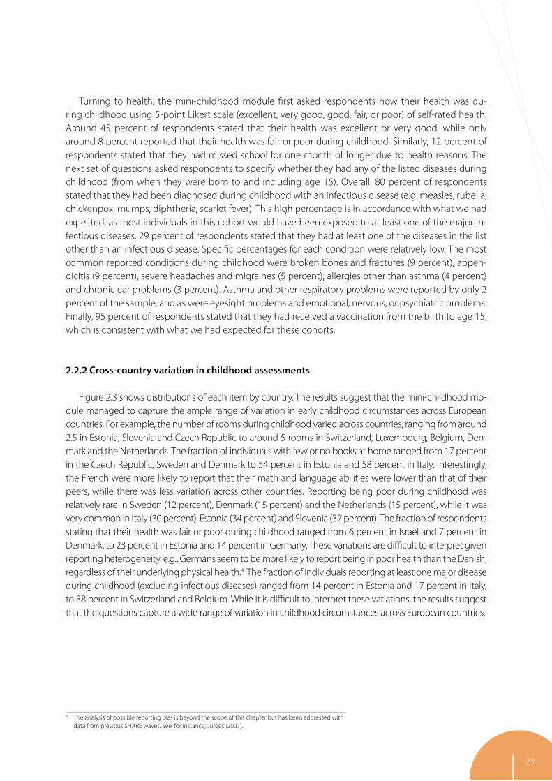
5 Interviewing interviewers: The SHARE interviewer survey 67
Julie M. Korbmacher, Sabine Friedel, Melanie Wagner, Munich Center for the Economics of Aging (MEA) at the Max Planck Institute for Social Law and Social Policy (MPISOC) Ulrich Krieger, University of Mannheim
6 Sample design and weighting strategies in SHARE Wave 5 75
Giuseppe De Luca, University of Palermo Claudio Rossetti, LUISS Guido Carli Frederic Malter, Munich Center for the Economics of Aging (MEA) at the Max Planck Institute for Social Law and Social Policy (MPISOC)
7 Item nonresponse and imputation strategies in SHARE Wave 5 85
Giuseppe De Luca, University of Palermo Martina Celidoni, University of Padua Elisabetta Trevisan, University of Padua & Netspar
8 Fieldwork monitoring and survey participation 101 in fifth wave of SHARE
Thorsten Kneip, Frederic Malter, Gregor Sand, Munich Center for the Economics of Aging (MEA) at the Max Planck Institute for Social Law and Social Policy (MPISOC)
9 Access to SHARE data and citation rules 158
Daniel Schmidutz, Munich Center for the Economics of Aging (MEA) at the Max Planck Institute for Social Law and Social Policy (MPISOC)
10 Measuring interview length with keystroke data 165
Johanna Bristle, Munich Center for the Economics of Aging (MEA) at the Max Planck Institute for Social Law and Social Policy (MPISOC)

8
1 SHARE Wave 5: Balancing innovation and panel consistencyAxel Börsch-Supan and Frederic Malter, Munich Center for the Economics of Aging (MEA) at the Max Planck Institute for Social Law and Social Policy (MPISOC)
This volume documents the most important questionnaire innovations, methodological advance-ments and new procedures introduced during the fifth wave of the Survey of Health, Ageing and Re-tirement in Europe (SHARE). SHARE’s main aim is to provide data on individuals as they age and their environment in order to analyse the process of individual and population ageing in depth. SHARE is a distributed European research infrastructure which provides data for social scientists, including demo-graphers, economists, psychologists, sociologists, biologists, epidemiologists, public health and health policy experts who are interested in population aging.
Covering the key areas of life, namely health, socio-economics and social networks, SHARE inclu-des a great variety of information: health variables (e.g. self-reported health, health conditions, physical and cognitive functioning, health behavior, use of health care facilities), bio-markers (e.g. grip strength, body-mass index, peak flow; and piloting dried blood spots, waist circumference, blood pressure), psy-chological variables (e.g. mental health, well-being, life satisfaction), economic variables (current work activity, job characteristics, opportunities to work past retirement age, sources and composition of cur-rent income, wealth and consumption, housing, education), and social support variables (e.g. assistance within families, transfers of income and assets, volunteer activities) as well as social network information (e.g. contacts, proximity, satisfaction with network). Researchers may download the SHARE data free of charge from the project’s website at www.share-project.org.
SHARE combines multi-disciplinarity with being genuinely multi-national. In Wave 5, we collected in-terview data from about 85,000 individuals aged 50 or over from 19 countries. Moreover, SHARE is har-monized with the U.S. Health and Retirement Study (HRS) and the English Longitudinal Study of Ageing (ELSA). Studies in Korea, Japan, China, India, and Brazil follow these models. Rigorous procedural guidelines, electronic tools, and instruments are designed to ensure an ex-ante harmonized cross-national design.
1.1 Innovations and methodology in Wave 5
This volume is divided into two sections. We first describe all innovations in questionnaire content and IT technology and then document the methodological procedures and updates of Wave 5, inclu-ding some new developments in methodological research.
Preparations for the design of the Wave 5 survey instrument were kicked off at a SHARE meeting in Budapest in late November 2011 when fieldwork of Wave 4 had just ended. All Area Coordinators presented first ideas that were then commented by the assembled country team leaders and the scien-tific monitoring board. This first input was discussed further at the January 2012 meeting of the SHARE Questionnaire Board and resulted in the first programming of a testable CAPI to be used in the pilot phase in March 2012.

9
At the outset of Wave 5, a conscious decision was made by the questionnaire board to invest a great deal of effort in revising existing questionnaire items and their response options and interviewer instruc-tions. Thus, one main goal of questionnaire development was a last round of improving longitudinal items to achieve a sustainable long-term standard of highest quality, sometimes sacrificing longitudinal consistency for improved measurement. Frederic Malter summarizes the outcome of these efforts in chapter 2 of this volume. Related to the efforts of improving existing items was the streamlining of a question-by-question encyclopedia (colloquially dubbed “Q-by-Q” by the SHARE community). In a nutshell, this encyclopedia is aimed at explaining concepts behind questionnaire items to facilitate proper translation and provide a last-resort help directory for interviewers. In Wave 5, for the first time, a streamlined version of the encyclopedia was implemented as part of the CAPI questionnaire and could be activated by interviewers. Anne Laferrère and Frederic Malter briefly describe the updated encyclopedia in chapter 2. The complete overhaul of the health care module by the responsible area coordinator, Hendrik Jürges, was also part of our efforts to achieve a sustainable long-term standard of highest quality. He wrote up the process and outcomes of this overhaul in his contribution to chapter 2.
As in all previous waves, the ultimate restriction of the development process was maintaining the same interview length while adding new content and amending existing items. The decision to admi-nister the Social Networks (SN) module only in Wave 6 again freed up about 5 minutes of interview time for new survey content. We used these “degrees of freedom” to accommodate a request that has gained momentum ever since the third wave of SHARE (SHARELIFE): administering at least part of the SHARE-LIFE questionnaire to those respondents who had not participated in Wave 3. Hence, a key innovation was the creation of a “miniature version” of the SHARELIFE questionnaire focussing on childhood events. Mauricio Avendano and Enrica Croda describe the process and outcome of this effort in chapter 2.
Along the lines of new content to be added, there was instant agreement at the meeting in Buda-pest that the financial crisis in 2008 and its massive and lasting implications for issues around demogra-phic change called for the allocation of available survey time to items on social exclusion and material deprivation. While SHARE already contained a number of financial items, the subjective side of poverty and social exclusion was perceived as needing a more refined assessment. Michał Myck, Monika Ocz-kowska and Dominika Duda provided details on the new items in their contribution to chapter 2.
Another mounting request, oftentimes brought up by SHARE users, finally gave birth to new survey items on better identifying the immigration status of SHARE respondents. We added questions that now allow conducting detailed analyses based on immigration status. Christian Hunkler, Gregor Sand, Morten Schuth and Thorsten Kneip wrote a brief overview of these efforts as part of the section on questionnaire innovation (chapter 2).
Three more important innovations are contained within this book. Despite our considerable experi-ence in devising high-quality IT systems, we learn during every wave how the software could be impro-ved – and actively seek input from the SHARE community – in user-friendliness and performance. A key improvement in software development was the introduction of a new database technology to avoid performance issues that arose in the last stages of Wave 4 due to high volumes of data to be synchro-nized between agency servers and Centerdata systems. Another crucial development was the revision and update of the online translation tool. Maurice Martens, Iggy van der Wielen, Arnaud Wijnant, and Gregor Sand summarize the updates to our IT technology in chapter 3.

10
Furthermore, our considerable experience in linking survey data to the administrative data of the German Pension Fund (DRV) has sparked interest and efforts in other countries to copy our success mo-del and enhance SHARE data in other countries as well. Julie Korbmacher and Daniel Schmidutz briefly illustrate the advances made on record linkage during Wave 5 in chapter 4.
The closing chapter of the innovation section comes from a project initiated in Wave 4 and extended in Wave 5. While we understand that in a face-to-face survey like SHARE the interviewer plays a crucial role in determining the many aspects of success of the study, we know remarkably little about how our interviewers feel about and approach their work in SHARE. To close this gap and move the research on interviewer effects in survey studies further ahead, we administered an interviewer survey to learn more about the attitudes and strategies of our interviewers. Julie Korbmacher, Melanie Wagner, Sabine Friedel and Ulrich Krieger lay out what we did and what we found in chapter 5.
The second section of this book gives all the details of the methodology of Wave 5. In chapter 6, Giu-seppe De Luca, Claudio Rosetti and Frederic Malter explain details on obtaining refreshment samples and how the sample designs determined the weighting. Their chapter also contained detailed informa-tion we assembled from the country teams on their sampling designs. In chapter 7, Giuseppe De Luca, Martina Celidoni and Elisabetta Trevisan wrote down how we dealt with the unavoidable issue of item non-response by applying imputation methods.
Thorsten Kneip, Frederic Malter, and Gregor Sand report in chapter 8 how the fieldwork was moni-tored and managed and what the ultimate outcomes were in terms of response and retention rates.
SHARE has an ever increasing number of users. While this is exactly what makes SHARE such a suc-cess, we are oftentimes confronted with difficult issues around granting access to the SHARE data. Da-niel Schmidutz has crafted chapter 9 to remove any remaining uncertainty as to how and why access to SHARE data is granted. He also describes our progress in obtaining Digital Objective Identifiers for released and to-be-released scientific use files.
This book is closed out with a contribution by Johanna Bristle on the measurement of interview length and how it differs by countries and subgroups. Hence, chapter 10 will be of particular relevan-ce to all researchers who are interested in conducting research with SHARE paradata or want to learn about conceptualizing interview length in general.

11
1.2 Management and organizational structure: The first ERIC ever
SHARE became the first European Research Infrastructure Consortium (ERIC) in March 2011 and – considered as implemented – was deemed a “success story” in the recent ESFRI Roadmap. SHARE had started as a pre-dominantly centrally financed enterprise. This was crucial for the harmonization across all member states. Data collection for waves one to three has been primarily funded by the European Commission through different framework programmes. Substantial additional funding came from the U.S. National Institute on Aging. With becoming an ERIC, national funding shall be dominant, but in order to achieve European Coverage for the project, central funding by the European Commission will remain a crucial factor for the sustainability of SHARE as a truly pan-European project.
In 2014 SHARE-ERIC moved its seat from Tilburg, the Netherlands, to Munich, Germany, to the Mu-nich Center for the Economics of Aging (MEA) within the Max Planck Institute for Social Law and Social Policy (MPISOC), the central coordination of SHARE.
SHARE-ERIC has now eleven members: Austria, Belgium, the Czech Republic, Germany, Greece, Italy, Israel, the Netherlands, Poland, Slovenia and Sweden, with Switzerland as Observer. Croatia, Denmark, Estonia, France, Hungary, Luxembourg, Portugal, and Spain are not yet members, but partner countries within the SHARE Consortium.
1.3 Acknowledgements
As in previous waves, our greatest thanks belong first and foremost to the participants of this study. None of the work presented here and in the future would have been possible without their support, time, and patience. It is their answers which allow us to sketch solutions to some of the most daunting problems of ageing societies. The editors and researchers of this book are aware that the trust given by our respondents entails the responsibility to use the data with the utmost care and scrutiny.
The country teams are the flesh to the body of SHARE and provided invaluable support: Rudolf Winter-Ebmer, Nicole Halmdienst, Michael Radhuber and Mario Schnalzenberger (Austria); Daniela Skugor, Bert Brockx, Martine Vandervelden and Karel Van den Bosch (Belgium-NL), and Stephanie Lin-chet, Jean-François Reynaerts, Laurent Nisen, Marine Maréchal, Xavier Flawinne, Jérôme Schoenmaeck-ers and Sergio Perelman (Belgium-FR); Radim Bohacek, Michal Kejak and Jan Kroupa (Czech Republic); Karen Andersen-Ranberg, Sonja Vestergaard and Mette Lindholm Eriksen (Denmark); Luule Sakkeus, Liili Abuladze, Tiina Tambaum, Enn Laansoo Jr., Kati Karelson, Ardo Matsi, Maali Käbin, Urve Kask, Ellu Saar, Marge Unt, Anne Tihaste, Lena Rõbakova and the whole team of GFK Custom Research Baltic, branch of Estonia who carried out the fieldwork (Estonia); Marie-Eve Joël, Anne Laferrère, Nicolas Bri-ant and Ludivine Gendre (France); Christine Diemand, Felizia Hanemann and Ulrich Krieger (Germany); Howard Litwin, Marina Motsenok and Lahav Karady (Israel), Guglielmo Weber, Elisabetta Trevisan, Chiara Dal Bianco, Martina Celidoni and Andrea Bonfatti (Italy); Maria Noel Pi Alperin, Gaetan de Lanchy, Nat-halie Lorentz, Jordane Segura and Jos Berghman (Luxembourg); Arthur van Soest, Frank van der Duyn Schouten, Johannes Binswanger, and Adriaan Kalwij (Netherlands); Michał Myck, Monika Oczkowska, Mateusz Najsztub, Dominika Duda (Poland); Pedro Mira and Laura Crespo (Spain); Josep Garre-Olmo,

12
Laia Calvò-Perxas, Secundí López-Pousa and Joan Vilalta-Franch (Spain, Girona); Gunnar Malmberg, Mi-kael Stattin, Filip Fors and Jenny Olofsson (Sweden); Carmen Borrat-Besson (FORS), Alberto Holly (IEMS), Peter Farago (FORS), Jürgen Maurer (IEMS), Michael Ingenhaag (IEMS), Boris Wernli (FORS) (Switzerland); Boris Majcen, Vladimir Lavrač, Saša Mašič and Andrej Srakar (Slovenia).
The innovations of SHARE rest on many shoulders. The combination of an interdisciplinary focus and a longitudinal approach has made the English Longitudinal Survey on Ageing (ELSA) and the US Health and Retirement Study (HRS) our main role models. We are grateful to James Banks, Carli Lessof, Michael Marmot and James Nazroo from ELSA; to Jim Smith, David Weir and Bob Willis from HRS; and to the members of the SHARE scientific monitoring board (Arie Kapteyn, chair, Orazio Attanasio, Lisa Berkman, Nicholas Christakis, Mick Couper, Michael Hurd, Annamaria Lusardi, Daniel McFadden, Norbert Schwarz, Andrew Steptoe, and Arthur Stone) for their intellectual and practical advice, and their continuing encouragement and support.
We are very grateful to the contributions of the four area coordination teams involved in the de-sign process. Guglielmo Weber (University of Padua) led the economic area with Agar Brugiavini, Anne Laferrère, Giacomo Pasini and Danilo Cavapozzi. The health area was led by Karen Andersen-Ranberg and assisted by Mette Lindholm Eriksen (University of Southern Denmark) with support from Simone Croezen at Erasmus University. Health care and health services utilization fell into the realm of Hendrik Jürges (University of Wuppertal). The fourth area, family and social networks, was led by Howard Litwin from Hebrew University with assistance from Kim Stoeckel, Anat Roll and Marina Motsenok.
The coordination of SHARE entails a large amount of day-to-day work which is easily understated. We would like to thank Kathrin Axt, Corina Lica, and Andrea Oepen for their management coordina-tion, Stephanie Lasson, and Hannelore Henning at MEA in Munich for their administrative support throughout various phases of the project. Martina Brandt, then Thorsten Kneip and Frederic Malter provided as assistant coordinators the backbone work in coordinating, developing, and organizing Wave 5 of SHARE. Preparing the data files for the fieldwork, monitoring the survey agencies, testing the data for errors and consistency are all tasks which are essential to this project. The authors and editors are grateful to Johanna Bristle, Christine Czaplicki, Christine Diemand, Fabio Franzese, Stefan Gruber, Felizia Hanemann, Christian Hunkler, Markus Kotte Julie Korbmacher, Gregor Sand, Daniel Schmidutz, Morten Schuth, Stephanie Stuck, Melanie Wagner, Luzia Weiss, and Sabrina Zuber for questionnaire de-velopment, dried blood spot logistics, data cleaning and monitoring services at MEA in Munich. We owe thanks to Giuseppe de Luca and Claudio Rosetti for weight calculations and imputations in Palermo and Rome. Finally, we are grateful for the help of our research assistants Judith Kronschnabl and Theresa Huck in getting this book ready for print.
Programming and software development for the SHARE survey was done by CentERdata in Tilburg. We want to thank Eric Balster, Marcel Das, Maurice Martens, Lennard Kuijten, Marije Oudejans, Iggy van der Wielen and Arnaud Wijnant for their support, patience and dedication to the project.
The fieldwork of SHARE relied in most countries on professional survey agencies: IFES (AT), CEL-LO, Univ. de Liège (BE), Link (CH), SC&C (CZ), TNS Infratest (DE), SFI Survey (DK), TNS (EE), TNS Demo-scopia (ES and sub-study in the Region of Girona), GfK-ISL (FR), Cohen Institute (IL), Ipsos (IT), CEPS-INSTEAD (LU), TNS NIPO (NL), Intervjubolaget (SE), and CJMMK (SI). We thank their representatives for an

13
extremely fruitful and innovative cooperation. We especially appreciate their constant feedback, the many suggestions, their patience in spite of a sometimes arduous road to funding, and their enthusiasm to em-bark innovative survey methods and contents. Much gratitude is owed to the nearly 2000 interviewers across all countries whose cooperation and dedication was, is and will be crucial to the success of SHARE.
Collecting these data has been possible through a sequence of contracts by the European Commis-sion and the U.S. National Institute on Aging, and the support by the member states.
The EU Commission’s contribution to SHARE through the 7th framework programme (SHARE-M4, No261982) is gratefully acknowledged. The SHARE-M4 project financed all coordination and networking activities outside of Germany. We thank, in alphabetical order, Ana Arana-Antelo, Peter Dro-ell, Philippe Froissard, Robert-Jan Smits, Maria Theofilatou, and Harry Tuinder in DG Research for their continuing support of SHARE. We are also grateful for the support by DG Employment, Social Affairs, and Equal Opportunities through Georg Fischer, Ralf Jacob and Fritz von Nordheim.
Substantial co-funding for add-ons such as the physical performance measures, the train-the-trai-ner program for the SHARE interviewers, and the respondent incentives, among others, came from the US National Institute on Ageing (P30 AG12815, R03 AG041397, R21 AG025169, R21 AG32578, R21 AG040387, Y1-AG-4553-01, IAG BSR06-11 and OGHA 04-064). We thank Richard Suzman and John Phil-lips for their enduring support and intellectual input.
The German Ministry of Science and Education (BMBF) financed all coordination activities at MEA, the coordinating institution. We owe special thanks to Angelika Willms-Herget, who also serves as chair of the SHARE-ERIC Council, and, in alphabetical order, Hans Nerlich, Ranyana Sarkar, Brunhild Spannhake and Beatrix Vierkorn-Rudolph who helped us with determination and patience to set up SHARE as a research infrastructure in Germany.
The core funding of Wave 5 came from national sources of the member states. We are grateful for the efforts it took to fund SHARE in each SHARE country, the perseverance of our ERIC delegates and ministry appointees in times in which funding social sciences and public health is all but trivial. Aus-tria (AT) received funding from the Bundesministerium für Wissenschaft und Forschung (BMWF) and acknowledges gratefully the support from the Bundesministerium für Arbeit, Soziales und Konsumen-tenschutz (BMASK). Belgium (BE) was funded by the Hercules foundation, an agency of the Flemish Government, the Fédération Wallonie-Bruxelles, the IWEPS, an agency of the Wallon Government, and the Belgian Federal Science Policy Administration. Switzerland (CH) received funding from the Swiss national science foundation (SNSF), grant number 10FI13_139514/1. The Czech Republic (CZ) recei-ved funding from the Ministry of Education, Youth and Sports. Germany (DE) received funding from the Bundesministerium für Bildung und Forschung (BMBF), Deutsche Forschungsgemeinschaft (DFG), Volkswagen Stiftung and the Forschungsnetzwerk Alterssicherung (FNA) of the Deutsche Rentenversi-cherung (DRV). Estonia (EE) received national funding from the Estonian Scientific Council, grant num-ber SF0130018s11, SF0130018s11AP and ETF 8325, grants No. 3.2.0601.11-0001 and 3.2.0301.11-0350 in the framework of the Research internationalisation programme through the Ministry of Education and Research and additional support by the Ministry of Social Affairs. Spain (ES) acknowledges grate-fully the financial support from DG-Employment, Bank of Spain and MINECO (Ministerio de Economía

14
y Competitividad, Subprograma de Actuaciones Relativas a Infraestructuras Científicas Internacionales, AIC10-A-000457) and the collaboration of Instituto Nacional de Estadística (INE). The Region of Girona in Catalonia (Spain) acknowledges gratefully the support from the Organisme de Salut Pública de la Diputació de Girona (DIPSALUT) and special thanks to the Institut d‘Assistència Sanitària de Girona (IAS) and the Institut d‘Estadística de Catalunya (IDESCAT) for their collaboration. In France (FR), Wave 5 has been financed jointly by Institut de recherche en santé publique (IReSP), Ministère de l‘enseignement supérieur et de la recherche (MESR), Caisse nationale de solidarité pour l‘autonomie (CNSA), Caisse nati-onale d‘assurance vieillesse (CNAV), Conseil d‘orientation des retraites (COR), Institut national de préven-tion et d‘éducation pour la santé (INPES) and Ecole des hautes études en sciences sociales (EHESS). The Israeli team (IL) received funding from the National Institute on Aging (U.S.) and the Ministry for Senior Citizens. In Italy (IT), funding for the fifth wave of SHARE was provided by the Ministry of University and Research (MIUR), in conjunction with the National Research Council (Consiglio Nazionale delle Ricerche - CNR), and by the following foundations: Fondazione Cassa di Risparmio di Padova e Rovigo and Forum ANIA Consumatori. Luxembourg (LU) received funding from the Ministère de l‘Enseignement Supérieur et de la Recherche du Luxembourg. Data collection in the Netherlands (NL) was funded by The Nether-lands Organisation for Scientific Research (NWO), The Dutch Ministry of Education, Culture and Science, by Netspar and Tilburg University. Portugal (PT) acknowledges the support of the Alto-Comissariado da Saúde (High Commissioner for Health). Sweden (SE) was supported by the Swedish Research Council. Slovenia (SI) received funding from the Ministry of education, science and sport.
SHARE is a great example how much power a research infrastructure can generate if - and only if - funders and researchers develop a common vision of improving the well-being of Europe’s citizens.

15
2 Questionnaire innovations in the fifth wave of SHARE
After Frederic Malter’s brief introduction of the general philosophy and work flow of developing the SHARE questionnaire, this chapter documents the key innovations, i.e. revised or completely new questionnaire content, of the fifth wave of SHARE. All contributing authors have been key actors in de-veloping or revising survey items and briefly outline the motivation that drove the new concepts, the basic ideas behind the measures and show some basic descriptive statistics that shed a first light on the possible use of the new variables.
Mauricio Avendano and Enrica Croda have laid out the compilation of a miniature version of ques-tionnaire of the third wave of SHARE that assessed the life histories of respondents (“SHARELIFE”). Due to the success of SHARELIFE, this so-called “mini-childhood” module was our response to the recurring requests by many SHARE researchers whose countries were not yet around in the third wave and where life histories were consequently missing for the entire sample.
Michal Myck and Monika Oczkowska and Dominika Duda have summarized the development of a set of items to extend the information content of SHARE in the area of material deprivation and social exclusion. The necessity for an in-depth measurement of material conditions and the multi-dimensional nature of exclusion in the 2013 wave has been a reaction to the need for better understanding of the welfare implications of the economic slow-down in Europe as well as a reflection of our concerns for international comparability of measures of welfare given the increasing heterogeneity of countries participating in the survey. The consequences of the economic crisis for the well-being of the 50+ population in many countries have been substantial, and understanding their broader implications has become an important element of SHARE’s academic effort.
Hendrik Juerges described the remake of the health care module that resulted in a more condensed way of harmonized institutional assessment across the participating countries. Much progress has been made in simplifying the content around health care with the result of better between-country comparability.
Christian Hunkler, Gregor Sand, Morten Schuth and Thorsten Kneip summarized the development of a series of items that will allow a more comprehensive assessment of a respondent’s migration and citizenship status.
Finally, Frederic Malter and Anne Laferrère briefly outline the development of an item encyclope-dia that has been missing from SHARE ever since its inception and finally entered the official SHARE production and release process during the fifth wave. Many SHARE researchers have been involved in generating this important tool and we are very grateful to them for their work and efforts. Especially translation of the upcoming sixth wave will benefit strongly from these efforts.

16
Item OK? yes
Do nothing
no
Part of a scale?
Do nothing Part of HRS/ELSA?
Harmoniza?on trumps item flaws?
Panel stability trumps item flaws?
Do nothing Revise
Do nothing
yes no
yes no
yes no
no yes
2.1 Questionnaire development in the fifth wave of SHARE Frederic Malter, Munich Center for the Economics of Aging (MEA) at the Max Planck Institute for Social Law and Social Policy (MPISOC)
One of the scientific aims of the SHARE study is to reconcile three opposing forces in question-naire development: 1) stability: keeping questionnaire items stable over time to enable panel analyses, 2) improvement: revising existing items based on new empirical evidence and 3) innovation: intro-ducing new content to facilitate research on emerging and timely topics and to remain scientifically “cutting edge”. This applies to all elements of a questionnaire item: the actual item wording, the response options, interviewer instructions and the item routing. Designing the questionnaire for any upcoming wave entails all three steps. In the case that a survey item gets slated for revisions, SHARE Questionnaire Board follows the decision tree shown in Figure 2.1 below. It can be seen that a SHARE item enters the process for revision only if all decision points in Figure 2.1 were negated.
Figure 2.1: Decision tree for revising existing SHARE items

17
Figure 2.2: Work flow new survey content in SHARE
In some cases, initially proposed changes to an existing survey item were abandoned to preserve panel stability. Likewise, many items in SHARE were harmonized with other longitudinal studies on aging (such as HRS and ELSA). In these cases even if some flaws have been identified in the process of data collection, the original item has been preserved to maintain cross-study harmonization. Finally, if the Questionnaire Board determines that the identified flaws are substantial enough to trump panel stability, the item enters the revision process. In the run-up to the fifth wave, the Questionnaire Board engaged in a general review of all SHARE items. In a number of cases minor changes were implemented to smooth the interview experience for interviewers and respondents (again, after following the general principle of Figure 2.1).
An example was streamlining the use of terms across items where it was deemed more important than maintaining panel stability. One item on individual income asked for income received “after any taxes or contributions”, while the subsequent item on household income asked for income “after any taxes”. After the streamlining process both included the expression “after any taxes or contributions”.
The more complicated set of questionnaire design tasks consisted in the introduction of new con-tent. The work flow from proposal to the final decision to field a new item is depicted in Figure 2.2 below.
The usual process concerning introduction of new content begins with discussion of potential items at SHARE management meetings. Once new content has been proposed and discussed by SHARE ex-perts from the specific field, it needs to be approved by the SHARE Questionnaire Board for inclusion in the pilot stage of SHARE. It was implemented in the source code of the generic English CAPI software. This generic CAPI instrument is then extensively tested by SHARE Central Coordination and – after a number of feedback loops with software developers (indicated with arrow A in Figure 2.2) – gets “fro-zen”. The frozen version of the generic instrument remains unchanged until the next development sta-ge. In addition, technical issues are slated for correction until the next stage (indicated by the sequential

18
feedback loop B in Figure 2.2). In the next step, the generic English questionnaire is imported into the online SHARE translation tool, the so-called “Translation Management Utility” (TMT, see chapter 3 for de-tails) so that national country teams can translate it into the survey fieldwork language. These country-specific (i.e. translated) CAPI instruments are then tested by the national teams in the same iterative fashion as the generic instrument (i.e. entailing feedback loops with software developers – indicated with the feedback loop C in Figure 2.2). In addition, problems that arise during translation, e.g. issues with the cross-cultural equivalence of question wording, are being fed back to the Questionnaire Board so that the generic English wording can be revised to achieve better cross-cultural applicability (indica-ted by the sequential feedback loop D in Figure 2.2). The entire process is repeated during the pretest stage of fieldwork which is the second round of testing before the actual main survey. After pretest data collection there is a final review of evidence around new items (e.g. variability, amount of missing data, length etc.) and the decision to keep or drop new content is made by the Questionnaire Board.
2.2 Measuring early childhood circumstances in SHARE Wave 5: A “mini childhood” moduleMauricio Avendano, London School of Economics and Political Science & Harvard School of Public Health Enrica Croda, Department of Economics, Ca’ Foscari University of Venice
Longitudinal surveys of ageing face the challenge of establishing how the lives of respondents be-fore entering the survey contribute to observed social, economic, health and well-being outcomes in later life. This is particularly important for surveys like SHARE, which start following people at older ages, as many of the crucial events experienced by respondents before entering the sample will be unknown to researchers, yet they are likely to be essential to understand late-life outcomes. This is a major chal-lenge for social sciences and policy as recent research increasingly highlights the importance of early life circumstances on later life outcomes.
To address this issue, after two waves of “classical” longitudinal data collection, the SHARE project entirely dedicated Wave 3, known as SHARELIFE, to the collection of retrospective life history data (Schröder, 2011). In the fourth wave SHARE returned to a “classical” longitudinal wave. The SHARELIFE questionnaire differed in several ways from the questionnaires of the regular waves by focusing on key events and changes individuals experienced before entering SHARE, using an Event History Calendar.1 SHARELIFE enables researchers to combine retrospective and contemporaneous/ prospective informa-tion and construct a panel dataset that tracked respondents from early childhood through adulthood. SHARELIFE has become a key element of SHARE that has sparked interest in areas that used to be impossible to study with concurrent information from ordinary waves. Obviously, SHARELIFE was col-lected only among respondents that had entered SHARE in either Wave 1 or Wave 2. This implies that for respondents that entered SHARE in Wave 4 and onwards no retrospective life history information was available. In addition, four new countries joined in the fourth wave and many “old” countries had added large refreshment samples in Wave 4 (see chapter 6 in this book). Many researchers involved with SHARE, emphasised their interest to repeat SHARELIFE for those new respondents absent in Wave 3. To fill this gap, the Wave 5 questionnaire design included a mini-childhood module that aimed to collect key information about early life socioeconomic and health circumstances for respondents who did not participate in SHARELIFE.
1 See Schröder, Ed. (2011) for further details on SHARELIFE Methodology.

19
In this chapter, we provide an overview of the mini-childhood module included in Wave 5. First, we discuss the questions selected as part of the module and provide an overview of descriptive statistics of these items. Second, we examine whether commonly observed associations between early childhood circumstances and late-life outcomes could be reproduced using the mini-childhood module applied in Wave 5. The module included questions concerning the health and socioeconomic status when the respondent was 10 years old, and questions on life circumstances from birth to age 15. Except for one, all questions were extracted from the original SHARELIFE questionnaire to enable comparability across the mini-childhood module and retrospective assessments for previous respondents. Due to questionnaire length constraints, however, the module only contained a selection of all SHARELIFE measures. This is due to the fact that, in addition to the mini-childhood module, Wave 5 included all regular assessments on respondent’s current circumstances. This chapter provides an overview of the reach and potential of the mini-childhood module applied in Wave 5 to examine early life circumstance and illustrate their importance for understanding late-life outcomes.
2.2.1 Overview of mini-childhood module
The aim of the mini-childhood module was to provide an overview of the early life circumstan-ces of older Europeans aged 50 and older, more specifically in the 14 European countries in which it was fielded (Austria, Belgium, Switzerland, Czech Republic, Germany, Denmark, Estonia, Spain, France, Italy, Luxembourg, Netherlands, Sweden, and Slovenia) and Israel. Unlike SHARELIFE, which focused on experiences over the entire life-course, this mini-module only focused on early childhood circum-stances for two reasons: first, the degree of detail required to assess full histories (e.g., of employment, health or financial difficulties) would demand a time-consuming interview that could not be carried out in combination with the regular SHARE Wave 5 modules, because it would exceed the questionnaire length constraints. In SHARELIFE early life circumstances were assessed using a set of crucial questions following the example of other surveys such as HRS and ELSA. Second, the mini-module was implemen-ted because experiences beyond childhood are undeniably essential in understanding older people’s life circumstances. There is an increasing interest in how experiences during childhood may be crucial in shaping individual’s later-life health, employment, earnings and social networks.2 The SHARE project offers a unique opportunity to assess these issues by collecting comparable data on early childhood experiences and linking them to health, employment, earnings and social networks in later life.
The mini-module maintained the different “periods of reference” for the different items in SHARELIFE and asked questions concerning the health, socioeconomic status and life circumstances when respon-dents were 10 years old and when respondents were growing up, from birth to age 15 (15 included). Specifically, survey participants were first asked about characteristics of the accommodation they lived in at the age of 10 (type of residence, number of rooms, number of people living in household, number of books), as well as self-rated levels of school performance (in math and in their country’s language) relative to peers at that age. Then they were asked about their socioeconomic status, with a question on family financial situation, health status, diagnoses of various illnesses and vaccinations during childhood from birth to age 15.
2 See, for instance, the collection of articles in Börsch-Supan, et al., Eds. (2011) and Brandt and Börsch-Supan, Eds. (2013).

20
All mini-childhood items replicate questions asked in SHARELIFE, so that researchers could have access to a harmonized set of variables for a large sample. The only exception is the question asking res-pondents whether they would say their family was financially well off, about average, or poor when they were growing up. This is a new question selected from HRS. It had not been asked in SHARE/SHARELIFE previously. We included it to capture overall socioeconomic status in childhood.3
The questions in the module were addressed only to respondents who had not had the opportu-nity to participate in SHARELIFE, mostly because they started participating to the SHARE project after SHARELIFE was fielded. There were 49,877 individuals that answered the module, corresponding to 77 percent of Wave 5 sample participants. Table 2.1 shows item non-response rates (missing answer or re-fusal) for each of the items included in the module. Similarly to the SHARELIFE experience, non-response rates were very low, ranging from 0.39 percent to 3.40 percent. The items thus seem to have functioned well as there was very limited non-response conditional on survey participation.
3 HRS uses 16 as cut-off age. The mini-childhood module uses age 15 in the wording for coherence with the other SHARELIFE questions.
Questionnaire item Item non-response rate %
Living in private residence at age 10 0.56
Rooms when 10 years old 2.14Number of people living in household when 10 1.41Number of books when 10 2.47Relative position to others mathematically when 10 1.44Relative position to others language when 10 3.40Financial position family from birth to age 15 0.48Childhood self-rated health status 0.39Missed school for 1 month+ 0.74Medical conditions during childhood (0-15) 0.86Vaccinations during childhood 1.02
Table 2.1: Item non-response in mini childhood module, SHARE Wave 5
Table 2.2 provides basic descriptive statistics of each of the items included in the mini-childhood module. Means and standard deviations of items are presented for items in four overall categories: characteristics of childhood accommodation; childhood school performance and cognitive abilities; childhood socioeconomic circumstances; and health-related items covering childhood self-rated over-all health, medical diagnoses during childhood, and access to vaccinations during childhood.
Around 92 percent of respondents reported to have lived in a private residence (a house of apartment the respondent or his parents or guardians owned or rented) at the age of 10. The average number of rooms was around 3.82, and the average number of household members was 5.57. 39 percent of respondents reported that there were few or no books at all at home when they were 10 years old and only 14 percent reported that there were more than a 100 books in their childhood home. 15 percent of respondents reported that

21
their math performance during school was worse than that of peers, while 13 percent reported worse perfor-mance in language during school compared to their peers. 19 percent of SHARE respondents reported that from birth to age 15, their family was poor, while 10 percent reported that their family was well-off.
Questionnaire item Mean SD
Childhood health (age 10)
Living in private residence at age 10 0.92 0.27
Rooms when 10 years old 3.82 1.95
Number of people living in household when 10 5.57 2.64
Number of books when 10 2.15 1.21
None or very few (0-10 books) 0.39 0.48
Enough to fill one shelf (11-25 books) 0.24 0.42
Enough to fill one bookcase (26-100 books) 0.22 0.41
Enough to fill two bookcases (101-200 books) 0.07 0.25
Enough to fill two or more bookcases (more than 200 books) 0.07 0.25
Childhood cognitive ability (age 10)
Relative position to others mathematically when 10
Better/much better 0.29 0.45
The same 0.56 0.49
Worse/much worse 0.15 0.35
Relative position to others language when 10
Better/much better 0.29 0.45
The same 0.57 0.49
Worse/much worse 0.13 0.34
Childhood SES (age 0-15)
financial position family from birth to age 15
Pretty well off financially 0.10 0.30
About average 0.45 0.50
Poor 0.19 0.39
It varied 0.01 0.11
Table 2.2: Descriptive statistics of mini-childhood module, SHARE Wave 5

22
Questionnaire item Mean SD
Childhood health (age 0-15)
childhood self-rated health status
Excellent 0.23 0.42
Very good 0.22 0.42
Good 0.22 0.41
Fair 0.06 0.24
Poor 0.02 0.13
It varied a great deal 0.00 0.05
Missed school for 1 month+ 0.12 0.33
Medical conditions during childhood (age 0-15)
Infectious disease 0.80 0.40
Polio 0.01 0.08
Asthma 0.02 0.14
Respiratory problems other than asthma 0.02 0.15
Allergies (other than asthma) 0.04 0.18
Severe diarrhoea 0.01 0.12
Meningitis/encephalitis 0.01 0.09
Chronic ear problems 0.03 0.16
Speech impairment 0.01 0.10
Difficulty seeing even with eyeglasses 0.02 0.16
Tuberculosis 0.01 0.10
Severe headaches or migraines 0.05 0.23
Epilepsy, fits or seizures 0.01 0.08
Emotional, nervous, or psychiatric problem 0.02 0.13
Broken bones, fractures 0.09 0.29
Appendicitis 0.09 0.29
Childhood diabetes or high blood sugar 0.00 0.03
Heart trouble 0.01 0.08
Leukemia or lymphoma 0.00 0.03
Cancer or malignant tumor (excluding minor skin cancers) 0.00 0.03
Access to basic preventive health care (age 0-15)
Vaccinations during childhood 0.95 0.21
Table 2.2: Descriptive statistics of mini-childhood module, SHARE Wave 5 (cont.)
23
Turning to health, the mini-childhood module first asked respondents how their health was du-ring childhood using 5-point Likert scale (excellent, very good, good, fair, or poor) of self-rated health. Around 45 percent of respondents stated that their health was excellent or very good, while only around 8 percent reported that their health was fair or poor during childhood. Similarly, 12 percent of respondents stated that they had missed school for one month of longer due to health reasons. The next set of questions asked respondents to specify whether they had any of the listed diseases during childhood (from when they were born to and including age 15). Overall, 80 percent of respondents stated that they had been diagnosed during childhood with an infectious disease (e.g. measles, rubella, chickenpox, mumps, diphtheria, scarlet fever). This high percentage is in accordance with what we had expected, as most individuals in this cohort would have been exposed to at least one of the major in-fectious diseases. 29 percent of respondents stated that they had at least one of the diseases in the list other than an infectious disease. Specific percentages for each condition were relatively low. The most common reported conditions during childhood were broken bones and fractures (9 percent), appen-dicitis (9 percent), severe headaches and migraines (5 percent), allergies other than asthma (4 percent) and chronic ear problems (3 percent). Asthma and other respiratory problems were reported by only 2 percent of the sample, and as were eyesight problems and emotional, nervous, or psychiatric problems. Finally, 95 percent of respondents stated that they had received a vaccination from the birth to age 15, which is consistent with what we had expected for these cohorts.
2.2.2 Cross-country variation in childhood assessments
Figure 2.3 shows distributions of each item by country. The results suggest that the mini-childhood mo-dule managed to capture the ample range of variation in early childhood circumstances across European countries. For example, the number of rooms during childhood varied across countries, ranging from around 2.5 in Estonia, Slovenia and Czech Republic to around 5 rooms in Switzerland, Luxembourg, Belgium, Den-mark and the Netherlands. The fraction of individuals with few or no books at home ranged from 17 percent in the Czech Republic, Sweden and Denmark to 54 percent in Estonia and 58 percent in Italy. Interestingly, the French were more likely to report that their math and language abilities were lower than that of their peers, while there was less variation across other countries. Reporting being poor during childhood was relatively rare in Sweden (12 percent), Denmark (15 percent) and the Netherlands (15 percent), while it was very common in Italy (30 percent), Estonia (34 percent) and Slovenia (37 percent). The fraction of respondents stating that their health was fair or poor during childhood ranged from 6 percent in Israel and 7 percent in Denmark, to 23 percent in Estonia and 14 percent in Germany. These variations are difficult to interpret given reporting heterogeneity, e.g., Germans seem to be more likely to report being in poor health than the Danish, regardless of their underlying physical health.4 The fraction of individuals reporting at least one major disease during childhood (excluding infectious diseases) ranged from 14 percent in Estonia and 17 percent in Italy, to 38 percent in Switzerland and Belgium. While it is difficult to interpret these variations, the results suggest that the questions capture a wide range of variation in childhood circumstances across European countries.
4 The analysis of possible reporting bias is beyond the scope of this chapter but has been addressed with data from previous SHARE waves. See, for instance, Jürges (2007).

24
0
1
2
3
4
5
6
EE SL CZ IL IT AT EE SE DE FR DK Nl CH LU BE
No. rooms at age 10
0
1
2
3
4
5
6
7
SE EE CZ DK DE AT LU IT FR SL CH BE EE IL Nl
No. household at age 10
0
0,05
0,1
0,15
0,2
0,25
LU EE SE DE CH IL AT BE EE CZ Nl IT DK SL FR
Worse in language
0
0,05
0,1
0,15
0,2
0,25
0,3
0,35
0,4
SE DK Nl BE LU FR IL CH DE EE AT CZ IT EE SL
Poor finances
0
0,05
0,1
0,15
0,2
0,25
SE Nl EE DK AT DE CH IL LU CZ SL IT BE EE FR
Worse in maths
0
0,1
0,2
0,3
0,4
0,5
0,6
0,7
CZ SE DK IL Nl CH EE DE BE LU AT FR SL EE IT
Few or no books at home at age 10
0
0,05
0,1
0,15
0,2
0,25
IL DK EE IT FR BE SL Nl SE CH AT LU CZ DE EE
poor_health
0
0,05
0,1
0,15
0,2
0,25
0,3
0,35
0,4
0,45
EE IT IL SL CZ AT FR LU EE DE DK Nl SE CH BE
Any diagnosis
Figure 2.3: Childhood circumstances by country, SHARE Wave 5

25
2.2.3 Mini-childhood module and adult outcomes
A key motivation to assess early childhood conditions is to understand to what extent they relate the late-life circumstances. While there is no established gold standard, one way to examine whether the mini-childhood module worked well is to examine whether previously observed associations in country-specific studies (e.g., Smith, 2009a; Smith 2009b) are reproduced in the overall SHARE sample. Table 2.3 shows results from several OLS models that examine the relationship between early childhood and the following adult out-comes: years of schooling, adult fair/poor health, height and long-term illness. In addition to early childhood variables, models include country fixed effects (omitted from Table), age and sex. A mixed picture emerges for accommodation characteristics: for example, living in a private residence at age 10 is associated with more years of schooling, but also with higher probability of reporting fair of poor health in adulthood. More rooms in the home residence during childhood is associated with higher adult height, while more people in the household (conditional on the number of rooms) is associated with lower height. The number of books during childhood is weakly associated with adult outcomes. Self-perceived poor math ability is associated with less height, while poor language ability is associated with higher probability of poor health.
The variable that most consistently predicts adult outcomes is the financial position of the family while growing up: those who reported that their family was poor ended up with less years of schooling, had higher prevalence of poor health and were more likely to report a long-term illness in adult life. Childhood health was also strongly related with health in adult life, with respondents reporting excellent health in childhood having a much lower probability of reporting poor health in adulthood. Early childhood health is also associ-ated with the risk of long-term illness, although this association is not statistically significant at conventional levels. Missing school during childhood for a month or more tends to imply a higher probability of long-term illness, but not with other outcomes. Surprisingly, having one or more medical diagnoses in childhood is associated with higher height, but also with higher risk of long-term illness in adult life. There was no clear relation between vaccinations during childhood and adult outcomes, although standard errors were large due to the small fraction of SHARE participants that had no vaccinations during childhood.

26
Years of schooling Adult poor health Height (cm) Long-term illness
Estimate SE Estimate SE Estimate SE Estimate SE
Age -0.0248 ** 0.0032 0.0142 ** 0.0012 -0.0566 ** 0.0172 0.0059 ** 0.0013
Male 0.1938 ** 0.0665 -0.0321 0.0251 10.5452 ** 0.3558 0.0220 0.0267
Childhood accommodation (age 10)
Living in private residence at age 10
0.2335 * 0.1161 0.1759 ** 0.0438 0.5505 0.6209 0.0801 0.0466
Rooms when ten years old
-0.0158 0.0246 -0.0155 0.0093 0.6713 ** 0.1309 0.0006 0.0098
Number of people living in household when ten
-0.0133 0.0131 0.0043 0.0049 -0.3731 ** 0.0700 0.0066 0.0053
Number of books when ten (reference category: > 200 books)
None or very few (0-10 books)
-0.2880 0.2387 0.0704 0.0900 -0.2627 1.2819 0.0382 0.0963
11-25 books -0.1441 0.2394 0.0625 0.0902 -0.0362 1.2843 -0.0353 0.0965
26-100 books -0.3567 0.2445 0.0883 0.0922 2.1682 1.3105 -0.0036 0.0985
101-200 books 0.1861 0.2997 0.0601 0.1130 3.3802 * 1.6012 -0.0109 0.1203
Childhood cognitive ability (age 10) (reference category: better/much better)
Relative position to others math
Worse/much worse -0.1689 0.1086 -0.0115 0.0409 -1.5754 * 0.5807 -0.0308 0.0436
The same 0.0757 0.0942 0.0167 0.0355 0.1668 0.5034 0.0317 0.0378
Relative position to others language
Worse/much worse -0.1814 0.1208 0.1541 ** 0.0455 -0.5339 0.6450 0.0889 0.0485
The same 0.0034 0.1009 0.0509 0.0380 0.3274 0.5376 -0.0294 0.0404
Table 2.3: OLS: Early childhood and adult social and health outcomes, SHARE Wave 5

27
Years of schooling Adult poor health Height (cm) Long-term illness
Estimate SE Estimate SE Estimate SE Estimate SE
Age -0.0248 ** 0.0032 0.0142 ** 0.0012 -0.0566 ** 0.0172 0.0059 ** 0.0013
Male 0.1938 ** 0.0665 -0.0321 0.0251 10.5452 ** 0.3558 0.0220 0.0267
Childhood accommodation (age 10)
Living in private residence at age 10
0.2335 * 0.1161 0.1759 ** 0.0438 0.5505 0.6209 0.0801 0.0466
Rooms when ten years old
-0.0158 0.0246 -0.0155 0.0093 0.6713 ** 0.1309 0.0006 0.0098
Number of people living in household when ten
-0.0133 0.0131 0.0043 0.0049 -0.3731 ** 0.0700 0.0066 0.0053
Number of books when ten (reference category: > 200 books)
None or very few (0-10 books)
-0.2880 0.2387 0.0704 0.0900 -0.2627 1.2819 0.0382 0.0963
11-25 books -0.1441 0.2394 0.0625 0.0902 -0.0362 1.2843 -0.0353 0.0965
26-100 books -0.3567 0.2445 0.0883 0.0922 2.1682 1.3105 -0.0036 0.0985
101-200 books 0.1861 0.2997 0.0601 0.1130 3.3802 * 1.6012 -0.0109 0.1203
Childhood cognitive ability (age 10) (reference category: better/much better)
Relative position to others math
Worse/much worse -0.1689 0.1086 -0.0115 0.0409 -1.5754 * 0.5807 -0.0308 0.0436
The same 0.0757 0.0942 0.0167 0.0355 0.1668 0.5034 0.0317 0.0378
Relative position to others language
Worse/much worse -0.1814 0.1208 0.1541 ** 0.0455 -0.5339 0.6450 0.0889 0.0485
The same 0.0034 0.1009 0.0509 0.0380 0.3274 0.5376 -0.0294 0.0404
Childhood SES (age 0-15)
Financial position family (reference category: pretty well off financially)
Poor -0.4951 ** 0.1762
About average -0.4443 ** 0.1674
Childhood health (age 0-15) (reference category: poor)
Childhood self-rated health status (1-5)
Excellent -0.4120 0.2174 -0.2369 ** 0.0819 1.0215 1.1578 -0.1170 0.0870
Very good -0.3549 0.2148 -0.1216 0.0810 1.5471 1.1438 -0.1514 0.0859
Good -0.3179 0.2116 -0.1118 0.0798 1.9790 1.1270 -0.1659 * 0.0847
Fair -0.1191 0.2427 -0.0363 0.0915 3.9618 ** 1.2931 -0.0743 0.0972
Missed school for 1 month+
-0.1289 0.1234 -0.0578 0.0465 -0.0329 0.6579 0.1250 * 0.0494
> 1 medical diagnosis (no infections)
-0.1587 0.0920 0.0115 0.0347 1.3180 ** 0.4909 0.1209 * 0.0369
Vaccinations du-ring childhood
0.1516 0.1210 -0.0748 0.0456 1.2021 0.6506 0.0027 0.0489
Table 2.3: OLS: Early childhood and adult social and health outcomes, SHARE Wave 5 (continued)

28
2.2.4 Conclusion
This chapter has validated the selection of items included in the mini-childhood module introduced in SHARE Wave 5 and provided an overview of its reach and potential to capture early life circumstance and illustrate their importance for understanding late-life outcomes. In particular, the new item on fa-mily financial circumstances while growing up performs particularly well as a measure of childhood socioeconomic status and strongly predicts adult health and social outcomes. Likewise, early childhood health strongly predicts adult health. Other items show similar associations as those observed with the original SHARELIFE sample and documented in Börsch-Supan, Brandt, Hank and M. Schröder, Eds. (2011). The mini-childhood module items capture a wide range of variation across countries in living and health circumstances across countries. An important area of future research is the extent to which early childhood measures are susceptible to reporting heterogeneity, in the same way that this ques-tion has been explored for adult measures, particularly for health. In conclusion, the mini-childhood module will provide for the first time researchers with a unique opportunity to examine how early childhood circumstance shape the life of older adults on the full range of SHARE countries in Europe.
ReferencesBörsch-Supan, A., Brandt, M., Hank, K. & Schröder, M. (Eds). (2011). The individual and the welfare state. Life histories in Europe. Heidelberg: Springer.
Brandt, M. & Börsch-Supan, A. (Eds). (2013). Advances in life course research. Special issue on: SHARELIFE - One century of life histories in Europe. 18 (1), pp. 1-114.
Jürges, H. (2007). True health vs response styles: exploring cross-country differences in self-reported health. Health Economics. 16 (2), pp. 163-178.
Schröder, M. (Ed). (2011). Retrospective data collection in the Survey of Health, Ageing and Retirement in Europe. SHARELIFE methodology. Mannheim: Mannheim Research Institute for the Economics of Aging (MEA).
Smith, J.P. (2009a). The impact of childhood health on adult labor market outcomes. The Review of Economics and Statistics. 91(3), pp. 478-489. doi:10.1162/rest.91.3.478.
Smith J.P. (2009b). Reconstructing childhood health histories. Demography. 46(2), pp. 387-403.

29
2.3 Innovations for better understanding deprivation and social exclusionMichał Myck, Monika Oczkowska and Dominika Duda, Centre for Economic Analysis (CenEA), Szczecin5
Both researchers and policy makers have long recognized that targets broader than simple measu-res of relative or absolute poverty ought to guide decisions in public policy with regard to welfare and well-being. In particular, one of the five key targets in the economic area for 2020 set by the European Commission refers to the concept of social exclusion with the aim to reduce the number of people at risk of social exclusion by 20 million people (European Parliament, 2010). While there is still dispute on what factors ought to be taken into account when measuring social exclusion, and how precisely this should be defined (see e.g. Levitas et al., 2007), there is growing evidence that the standard measures of income-based poverty are a poor indicator for well-being (Nolan and Whelan, 1996; Adena and Myck, 2014). Current income is an imperfect proxy of material conditions and may poorly reflect on a number of important aspects of well-being. This may be particularly important in the case of older individuals, given the importance of such issues as health, disability and social interactions in later life. Substantial body of research has indicated that due to exit out of the labour market, deteriorating health and limits on the ability to participate in social life, older individuals are at high risk of deprivation in the material and social domains (see e.g. Jehoel-Gijsbers and Vrooman 2007, 2008; Levitas et al., 2007). Understan-ding the variation in their well-being and consequences of ageing for deprivation and social exclusion requires a comprehensive approach and a set of tools to support the analysis.
In reaction to the growing need for better understanding of material conditions and broader mul-tidimensional aspects of social exclusion, the Wave 5 SHARE questionnaire was supplemented with a number of questions specifically designed for this purpose. The standard SHARE questionnaire from waves 1, 2 and 4 covers a broad number of aspects of material conditions, such as income sources and assets owned by respondents and specific financial difficulties they may have. SHARE questionnaires included also some variables reflecting subjective assessment of household’s financial situation and the level of some basic expenditures. Wave 2 also included information on housing and perceived quality of the neighbourhood. Thus, while various aspects of the broader concept of “quality of life” have always been present in SHARE, the amount of information gathered with regard to material conditions and social exclusion was deemed unsatisfactory and motivated the development of new indicators which we describe in this chapter.
The extension of the standard questionnaire was conducted under the SHARE-M4 project financed through 7th Framework Programme and prepared for implementation in Wave 5 of SHARE. This exten-sion was developed as a specific work package of the project (“European 50+ Exclusion Module”) in cooperation with several institutional nodes of the SHARE Consortium, including in particular the Centre for Economic Analysis (CenEA), the Hebrew University (Jerusalem), University of Venice and the Munich
5 This chapter documents the development of the so called „European 50+ Exclusion Module” implemented in the Wave 5 of the SHARE survey. Work on this module was conducted as part of the EU Framework 7 programme “SHARE-M4” project (Work Package 16) realized between January 2011 and December 2014. The development of the additional set of questions benefited from numerous contributions of members of the SHARE consortium, and participants in a number of SHARE project progress meetings. The authors also want to acknowledge the contribution of Zuzanna Pogorzelska in the early stage of the module’s development and are grateful for the possibility to discuss the options for the module with Panos Demakakos (UCL, ELSA) and Matt Barnes (NatCen).

30
Centre for the Economics of Ageing (MEA). The principal aim of this new set of questions was to pro-vide additional informative measures of respondents’ material situation suitable for the multi-country nature of SHARE and to supplement them with additional information which would allow developing multidimensional measures of social exclusion. The development of the specialized set of items was conducted in a number of stages, which are briefly described below, and in the end resulted in 19 additional items of the questionnaire covering such aspects as affordability of specific expenses and neighbourhood quality (see Table 2.4 for a detailed list).
2.3.1 Questionnaire development
Questionnaire items which focus on deprivation and exclusion were developed in several stages starting with a review of existing poverty, deprivation and exclusion items in other surveys. Particularly the SHARE “sister” surveys, HRS and ELSA, or those specifically focusing on material conditions provided valuable input: the European Survey on Income and Living Conditions (EU-SILC), the Family Resources Survey in the UK and a survey specifically designed to address poverty and social exclusion in Northern Ireland: Monitoring Poverty and Social Exclusion (for more details on content directed on social exclu-sion in each study see: HRS – Smith et al., 2013; ELSA – Barnes et al., 2006; PSE in Northern Ireland – Hill-yard et al., 2003; EU-SILC – European Commission, 2014; FRS – McKay and Collard, 2003).
Initially the additional set of questions was planned as a special paper-and-pencil (“drop-off”) ques-tionnaire handed to respondents after completing the main CAPI survey. The draft version of this ques-tionnaire was presented to the SHARE Consortium and the Questionnaire Board and discussed in detail at the SHARE progress workshop in November 2011. Recognising the importance of the issues ad-dressed by these additional questions, in particular at the time of the prolonged economic downturn in Europe, the Consortium decided to incorporate the additional questions in the main CAPI survey.
A second round of analysis and consultation followed to identify the most valuable items from the initial list to be incorporated into the CAPI questionnaire. As a result, a battery of questions considered as most helpful in measuring different aspects of material conditions and social exclusion was tested at the pilot stage of the survey in 16 countries in March 2012 and then again during the pretest stage of the fifth wave in June and July of the same year. Data collected during the pretest served as guidance for choosing the final set of questions which were most effective in capturing different aspects of de-privation and social exclusion. The most valuable items were incorporated into main generic Wave 5 questionnaire and translated into country specific versions which went into the field in 15 countries (Portugal dropped out of Wave 5 after the pretest).

31
2.3.2 New social exclusion items included in SHARE Wave 5
Table 2.4 on the next page presents details of the final set of additional 19 questions. The first column contains the coding and label of a question, next the wording of the question, and the principal other studies which contain this or very similar item. Most of the questions in the exclusion set were asked of only one person in the household (the so-called “household respondent”) as exclusion, in particular in the material and neighbourhood dimensions, was treated a characteristic of the entire household. The last column in the table gives information on number of households that provided valid answers to given questions.
Broadly, and in line with many studies in the literature on social exclusion, the set of exclusion ques-tions can be divided into the following two categories: • affordability and living costs; • neighborhood quality.
2.3.3 Exclusion questions - sample coverage
At the time the decision was made to include the additional exclusion questions into the main CAPI interview, the questions were supposed to be asked only of a subsample of about half of longitudinal respondents. However, given the prolonged duration of the economic downturn and the consequent increasing importance of evidence concerning material deprivation and social exclusion, the coverage of these questions was extended just before the start of the main stage of the survey to include all longitudinal households and also the refreshment samples. Unfortunately, given the complex coding structure of the questionnaire routing, an element of the interview design went unnoticed at this final stage of the questionnaire development and as a result the final coverage of the exclusion set of ques-tions is at about 94 percent. While incomplete, this is much higher than initially planned. In the case of refreshment households the main reason for incomplete coverage was households in which the role of the “household respondent” (who received the exclusion set of questions) was taken by the spouse of the person drawn into the sample. Similarly, the principal cause behind incomplete coverage among longitudinal households was cases where a new member of the household took on the role of the “household respondent”. In these cases, the “household respondent” was not part of the gross sample through which coverage of the exclusion questions was identified and as a result the exclusion informa-tion for these households was missing. Given additional routing and item non-response, the absolute number of valid answers to the 19 exclusion questions in households varies between 40 341 and 41 237 (see Table 2.4). Coverage of exclusion questions by country varies between 83 percent (in Czech Republic) and 99 percent (in Switzerland) mainly as a consequence of different sizes of the refreshment samples. The routing was changed in the case of Luxembourg which went late into the field and this ensured 100 percent coverage.

32
Table 2.4: Questions in the European 50+ Exclusion Module of SHARE Wave 5
Category Question code and label Question text Response options
Other studies using this or similar item
Number of households with valid answers
Nei
gh
bou
rhoo
d q
ualit
y
CO201_AffordGroceries
Can your household afford to regularly buy necessary groceries and household supplies?
1. Yes 5. No PSE NI 41 158
CO202_AffordHoliday
Could your household afford to go for a week long holiday away from home at least once a year?
1. Yes 5. No EU-SILC, FRS 41 053
CO206_AffordExpense
Could your household afford to pay an unexpected expense of [AffordExpenseAmount] without borrowing any money?(A)
1. Yes 5. No EU-SILC 40 934
CO207_PovertyWornOutClothing
Please think of your financial situ-ation over the last twelve months. In the last twelve months, to help you keep your living costs down, have you... …continued wearing clothing that was worn out because you could not afford replacement?
1. Yes 5. No PSE NI 41 129
CO208_PovertyWornOutShoes
… continued wearing shoes that were worn out because you could not afford replacement?
1. Yes 5. No PSE NI 41 140
CO209_PovertyPutUpWithCold
… put up with feeling cold to save heating costs?
1. Yes 5. NoPSE NI, EU-SILC, FRS
41 165
CO211_PovertyPostponedDentist
… postponed visits to the dentist?
1. Yes 5. No PSE NI 41 182
CO213_PovertyGlasses
… gone without or not replaced glasses you needed because you could not afford new ones?
1. Yes 5. No PSE NI 41 172
CO020_HowMuchNeeded (B)
Which minimum amount of mo-ney in total would your household need per month to easily make ends meet?
amount EU-SILC 26 192(B)
BR033_MeatAfford
Would you say that you do not eat meat, fish or chicken more often because...
1. you cannot afford to eat it more often 2. for other reasons
PSE NI, EU-SILC
41 232
BR034_FruitAfford
Would you say that you do not eat fruits or vegetables more often because ...
1. you cannot afford to eat it more often 2. for other reasons
PSE NI, EU-SILC
41 237

33
Category Question code and label Question text Response options
Other studies using this or similar item
Number of households with valid answers
Nei
gh
bou
rhoo
d q
ualit
y
HH022_LocalFeelPart
I really feel part of this area. Would you say you strongly agree, agree, disagree or strongly disagree?
1. Strongly agree 2. Agree 3. Disagree 4. Strongly disagree
HRS 40 988
HH023_LocalVandalism
Vandalism or crime is a big problem in this area.
1. Strongly agree 2. Agree 3. Disagree 4. Strongly disagree
HRS, EU-SILC 40 929
HH024_LocalClean
This area is kept very clean.
1. Strongly agree 2. Agree 3. Disagree 4. Strongly disagree
HRS, EU-SILC, PSE NI
41 040
HH025_LocalPeopleHelpful
If I were in trouble, there are people in this area who would help me.
1. Strongly agree 2. Agree 3. Disagree 4. Strongly disagree
HRS 40 341
HH027_LocalBank
How easy is it to get to the nearest bank or cash point?
1. Very easy 2. Easy 3. Difficult 4. Very difficult
ELSA 40 964
HH028_LocalGroceryShop
How easy is it to get to the nearest grocery shop or supermarket?
1. Very easy 2. Easy 3. Difficult 4. Very difficult
ELSA 41 100
HH029_LocalGeneralPractitioner
How easy is it to get to your general practitioner or the nearest health centre?
1. Very easy 2. Easy 3. Difficult 4. Very difficult
ELSA 41 070
HH030_LocalPharmacy
How easy is it to get to the nearest pharmacy?
1. Very easy 2. Easy 3. Difficult 4. Very difficult
41 102
Table 2.4: Questions in the European 50+ Exclusion Module of SHARE Wave 5 (continued)
(A)- [AffordExpenseAmount] - specified in each country to correspond to the monthly country specific relative poverty line defined as 60 percent of equalized median income.
(B)- item asked in all households provided they report that they do not “make ends meet easily” in question CO007_. Questions asked only of respondents in private households covered by the SE set of questions. “Number of households with valid answers” includes households for which a valid answer has been given in the interview or can be imputed using the interview routing rules. For example additional routing rules apply to affordability of food items (BR033 and BR034). These are asked only if respondent eats meat (or fruit and vegetables) less often than 3 times a week, which is respectively in 8763 and 3086 cases. Those who eat them 3 times a week or more often (and are covered by other exclusion questions) can be imputed as being able to afford it.

34
The value of the “unexpected expense” in (2) was specified in each country to correspond to the country-specific relative poverty line defined as 60 percent of the median household equivalised monthly disposable income. Overall, nearly every third respondent could not afford a holiday and every fourth the unexpected expense. The item asking for keeping costs down by postponing a dentist’s visit was confirmed in about 10 percent of all households. The proportion of disadvantaged households va-ries significantly by country. The highest share of households reporting problems with affordability of all three items is in Estonia, where over 70 percent of households could not afford holiday, 51 percent – an unexpected expense and 35 percent - a dentist visit. On the other hand in Luxembourg 11 percent of households could not afford holiday, 13 percent - an unexpected expense and 4 percent - dentist visit.
2.3.4 Initial findings in main stage of SHARE Wave 5
Figures 2.4 and 2.5 present results on a selected number of the exclusion items by country based on an internal release of SHARE Wave 5 data. Figure 2.4 shows the proportion of households who reported that they:
1) “cannot afford a week long holiday away from home at least once a year”, 2) “cannot afford an unexpected expense without borrowing”,3) “postponed visits to the dentist in order to keep living costs down”.
Figure 2.4: Share of households with difficulties to afford holiday, unexpected expense and dentist visitsSource: SHARE Wave 5 internal release 0-0-7. Weighted data. See Table 2.5 for details.

35
Figure 2.5 displays the percentage of households who declared that they did not eat meat (or fish, chicken) or fruits (or vegetables) three times a week or more often because they could not afford it. The aim of these questions was to identify the households in severe material difficulties and, as ex-pected, the proportion of households considered deprived according to these criteria is much lower. On average only 2 percent of all households couldn’t afford eating meat and 1 percent couldn’t afford fruits and vegetables. There is a lot of cross-country variation in these rates, however, with much higher proportion of households in countries such as Estonia, where 8 percent of households could not afford meat and 3 percent could not afford fruits, Italy (respectively 7 percent and 2 percent) and the Czech Republic (5 percent and 2 percent).
Figure 2.5: Share of households who do not eat meat or fruits and vegetables more often than twice a week because
they cannot afford to
Source: SHARE Wave 5 internal release 0-0-7. Weighted data. See Table 2.4 for details.Notes: “meat” – household cannot afford to eat meat at least three times a week; “vegetables” - household cannot afford to eat fruits or vegetables at least three times a week. Denominator includes households that either eat meat/fruits more often than twice a week or that do not eat meat/fruits more often because of other reasons.
2.3.5 Conclusion
Effective policy making in the area of poverty alleviation and social inclusion among the 50+ requi-res continuous efforts to understand the nature of the underlying problems and appropriate tools to monitor their scale and dynamics. In SHARE Wave 5 a new set of questions was included in the interview to capture material and social aspects of deprivation of older people in Europe. This set of 19 questions extends the potential of SHARE to serve as a reference dataset for analysis of deprivation and social ex-clusion and these new interview items should help researchers in designing comprehensive measures of these phenomena. Development of such measures will shed new light on the variation in depriva-tion across countries and can point towards policies which could be effective in reducing the scale of different aspects of deprivation among the 50+ in Europe.

36
ReferencesBarnes, M., Blom, A., Cox K. & Lessof, C. (2006). The social exclusion of older people: evidence from the first wave of the English Longitudinal Study of Ageing (ELSA). Office of the Deputy Prime Minister.
European Commission (2014). Methodological guidelines and description of EU-SILC target variables.
European Parliament (2010). Resolution on EU 2020. Brussels.
Hillyard, P., Kelly, G., McLaughlin, E., Patsios, D. & Tomlinson, M. (2003). Bare necessities. Poverty and Social Exclusion in Northern Ireland: key findings. Democratic Dialogue.
Jehoel-Gijsbers, G. & Vrooman, C. (2007). Explaining social exclusion. A theoretical model tested in the Netherlands. The Netherlands Institute for Social Research.
Jehoel-Gijsbers, G. & Vrooman, C. (2008). Social exclusion of the elderly: a comparative study of EU Mem-ber States. ENEPRI Research Report No. 57.
Levitas, R., Pantazis, C., Fahmy, E., Gordon, D., Lloyd, E. & Patsios D. (2007). The multi-dimensional analysis of social exclusion. University of Bristol.
Maja, A. & Myck, M. (2014). Poverty and transitions in health in later life. Social Science & Medicine. 116, pp. 202–210.
McKay, S. & Collard, S. (2003). Developing deprivation questions for the Family resources survey. Working Paper Number 13. University of Bristol.
Nolan, B. & Whelan, C.T. (1996). Measuring poverty using income and deprivation indicators: alternative approaches. Journal of European Social Policy. 6(3), pp. 225-240.
Smith, J., Fisher, G., Ryan, L., Clarke, P., House, J. & Weir, D. (2013). Psychosocial and Lifestyle Questionnaire 2006 – 2010. Documentation Report. University of Michigan.

37
2.4 Health care utilization and out-of-pocket expensesHendrik Jürges, University of Wuppertal
To understand the recent innovations of the fifth wave in the health care module in SHARE, it is useful to briefly recount its history of the health care module. This short but important module serves to facilitate international comparisons in two areas: (1) health care utilization (in the last 12 months), including unmet need, and (2) health insurance coverage and out-of-pocket expenses. Despite some progress, cross-national harmonization of questions asked in SHARE continues to be one of the major design challenges, in particular with regard to institutional differences in health care or pension sys-tems. Two principal approaches to harmonization have been discussed and used in SHARE from the very beginning: ex-post and ex-ante harmonization. In general, SHARE aims at implementing ex-ante harmonization whenever possible.
With ex-post harmonization, questions or sets of questions are designed to best cover the institutio-nal details in a specific country without regard to the formulation of these questions in other countries. Whereas this approach has the undisputable advantage of allowing for the tailoring of the questionnaire to the best understanding of the individual respondent in each country, ex-post harmonized questions require individual data users to have detailed institutional knowledge on each country’s health care system in order to make questionnaire content comparable for cross-country analysis. In the past, large teams of researchers were needed (and funded) to complete this task on a case-by-case basis using dif-ferent surveys from different countries. In its first wave, the SHARE health care module has followed the ex-post harmonization approach with respect to content such as health insurance coverage. However, programming and testing a CAPI instrument with intricate country-specific routing has proved to be complicated, time-consuming, and error-prone. Moreover, individual data users not familiar with the details of the country specific routing had difficulty understanding which questions were asked or not asked in what country and for which reasons.
In contrast, ex-ante harmonized questions follow a generic template that aims at covering structural similarities or similar concepts between health care systems. They are designed to allow researchers with knowledge of these structural characteristics to use the data without needing detailed instituti-onal knowledge on each country used in their analysis. Researchers from each country are needed in the design phase to word survey items which will be understood by a typical respondent, i.e. a person with about eight years of formal schooling. For instance, whereas the concept of a private health insu-rance is usually understood by researchers in health systems research, questions regarding whether a respondent has purchased supplementary or private or complementary health insurance need to be phrased in country-specific language. Obviously, literal translation of technical terms has the potential to confuse respondents. Because of the difficulties of the ex-post harmonization approach experienced during the first wave of the survey, particularly in the design and programming stages, SHARE has shif-ted to ex-ante harmonization in the second wave. However, when designing those questions, ensuring longitudinal comparability of the questionnaire was difficult as well, and eventually resulted in a longer and more repetitive module than intended. Problems were encountered particularly with respect to questions on health insurance coverage, and the compromises found still left some room for improve-ment in both the researchers’ and the respondents’ view.

38
Eventually, the challenges encountered in the first two waves led to a partial restart of the health care module. Wave 3 (SHARELIFE) did not contain the standard health care module due to the very nature of the survey, which was collecting retrospective life histories instead of “regular” panel. In Wave 4, due to time-consuming innovations in other parts of the survey, a short version of the module that contained only questions on health care utilization (e.g. doctor visits, hospital stays) that – although they face general methodological challenges due to potential recall error – have proved to be quite unproblematic in cross-national comparability.
The design of the health care module in SHARE Wave 5 was guided by three principles. First, based on our earlier experience we decided to stick to the ex-ante harmonization of our questionnaire. As an improvement vis-a-vis earlier waves, detailed question-by-question instructions (see also chapter 2.6) that explained key health care and health economics concepts in English were given to translators and country teams to ensure that all terms were translated correctly. Direct communication between Area Coordinator and Country Teams ensured that all concepts were well understood and translated, solving all remaining instances of ambiguity. Second, those questions on health care utilization that have worked well in all previous waves of SHARE would be largely unaltered to ensure longitudinal comparability. Third, the idea to measure the degree of health insurance coverage individually in nearly 20 different countries with 20 different health care systems was abandoned. Rather, the aim of the cur-rent health care module was to measure as precisely as possible what health insurance did not cover: out-of-pocket expenses. With such a measure at hand, it will be possible to compute the monetary burden of gaps in health insurance coverage, for instance as percentage of individual income. To impro-ve our measure of out-of-pocket expenses, we decided to ask for expenses for each type of utilization separately (physician visits, hospital stays, medication, dentist visits, other inpatient stays, at-home care), resulting in the following general sequence of questions:
• In the last twelve months, have you had health care of type X?• If yes: Did you pay anything out of pocket for your health care of type X?• If yes: In the last 12 months, how much did you pay overall for your health care of type X?
Table 2.5 on the next page gives an overview of all items of the health care module of SHARE Wave 5. A more detailed account how to use those SHARE Wave 5 variables to compute out-of-pocket expenses is given in the Appendix 1. Appendix 2 shows a basic breakdown of out-of-pocket expenses by country.

39
Variable Question text Response options Filter
A. Doctor visits
HC002
Now please think about the last 12 months. About how many times in total have you seen or talked to a medical doctor or qualified nurse about your health? Please exclude dentist visits and hospital stays, but include emergency room or outpatient clinic visits.
Number of visits (Integer)
HC082
Did you pay anything out of pocket for your doctor vi-sits [past your deductible] (in the last twelve months)? Please also include expenses for diagnostic exams, such as imaging or laboratory diagnostics.
1. Yes 5. No IF HC002>0
HC083 How much did you pay overall for your doctor visits (in the last twelve months)?
Amount in local currency (Integer) IF HC082==1
B. Medication
HC088
Earlier we talked about medication you may take. In the last twelve months, did you pay anything out of pocket for your medication [past your deductible]? Please inclu-de both drugs that were prescribed by your doctor and those you bought without prescription.
1. Yes 5. No
HC089 About how much did you pay overall for drugs [past your deductible] in the last twelve months?
Amount in local currency (Integer) IF HC088==1
HC130 Can you tell me about how much you pay for your medication in a typical month?
Amount in local currency (Integer)
IF HC089==DK
C. Dentist visits
HC010 During the last twelve months, have you seen a den-tist or a dental hygienist?
1. Yes 5. No
HC092
In the last twelve months, did you pay anything out of pocket for your dental care [past your deductible]? Please include payments for diagnoses, treatments, and dental prostheses.
1. Yes 5. No IF HC010==1
HC093 How much did you pay overall for your dentist care [past your deductible] in the last twelve months?
Amount in local currency (Integer) IF HC092==1
D. Stays in hospitals and other care facilities
HC012During the last twelve months, have you been in a hospital overnight? Please consider stays in medical, surgical, psychiatric or in any other specialised wards.
1. Yes 5. No
HC013 How many times have you been a patient in a hospi-tal overnight during the last twelve months? Number of stays (Integer) IF HC012==1
HC014 How many nights altogether have you spent in hospi-tals during the last twelve months?111
Number of nights (Integer) IF HC012==1
HC064
During the last twelve months, have you been a patient overnight in any health care facility other than a hospital, for instance in institutions for medical reha-bilitation, convalescence, etc.? Please do not include stays in nursing homes/residential care facilities.
1. Yes 5. No
HC066How many nights altogether have you spent in any institution other than a hospital or a nursing home during the last twelve months?
Number of nights (Integer) IF HC064==1
HC094 Did you pay anything out of pocket for your stays in hospitals and other health care facilities in the last twelve months?
1. Yes 5. No
IF HC012==1 OR HC064==1
Table 2.5: Overview of questions on health care utilization and out-of-pocket-expenses in SHARE Wave 5

40
Note, however, that by deliberately not trying to measure health insurance coverage, we decided that our data will not be suitable to study the incentive effects of health insurance on utilization and subsequent health outcomes. It would be very useful to be able to exploit cross-national differences in coverage to stu-dy its effect on the well-being of the older population. Alas, this aim proved too ambitious in a survey like SHARE, which is not specialized on health care but has to accommodate much scientific content in limited survey time. Still, we collected supplementary information on health insurance coverage that might be use-ful to social policy makers and researchers. We included one question on satisfaction with health insurance coverage in the statutory health insurance or the respective national health system and two questions on subjective unmet need. In addition, two further questions on unmet need regarding dentist visits and wea-ring glasses were asked in other parts of the SHARE survey.
Table 2.5: Overview of questions on health care utilization and out-of-pocket-expenses in SHARE Wave 5 (continued)
Variable Question text Response options Filter
HC095How much did you pay overall for your hospital stays in the last twelve months?
Amount in local currency (Integer) IF HC094==1
E. Care received at home
HC127
During the last twelve months, did you receive in your own home any professional or paid services listed on card 40 due to a physical, mental, emotional or memo-ry problem?
1. Help with personal care2. Help with domestic tasks3. Meals-on-wheels4. Help with other activities96. None of the above
HC128In the last twelve months, did you pay anything out of pocket for the services listed on card 40?
1. Yes 5. No
IF HC127==1
HC129
How much did you pay overall for personal care, domestic tasks, meals on wheels or other help in the last twelve months? Please do not include expenses reimbursed by a health or long-term insurance.
Amount in local currency (Integer)
IIF HC128==1
F. Temporary stays in nursing homes
HC029During the last twelve months, have you been in a nursing home/residential care facility overnight?
1. Yes, temporarily3. Yes, permanently5. No
IF MN024==5
HC031 During the last 12 months, how many weeks altogether did you stay in a nursing home?
Number of weeks (integer)
IF HC029==1
HC096
Did you pay anything out of pocket for nursing home stays in the last twelve months? [To remind you, by out of pocket payments we mean payments not reim-bursed by your long-term care insurance.]
1. Yes 5. No
IF HC029==1
HC097How much did you pay overall for your nursing home stays in the last twelve months?
Amount in local currency (Integer)
IF HC096==1
G. Deductible
HC111
Does your own coverage in your basic health insurance/national health system have a deductible, that is, do you have to pay up to a fixed amount for your health care yourself before benefits of the policy can apply?
1. Yes 5. No
HC112About how large was your annual deductible in the last calendar year?
Amount in local currency (Integer)
IF HC111==1

41
Overall, the SHARE health care module in Wave 5 provides a workable compromise between scien-tific ambition, technical feasibility and respondents’ interest. Changes between waves 5 and 6 will be minimal. While data on health care utilization were comparable across waves since Wave 1, the health care module will now provide much needed longitudinal insight into the elders’ financial burden of health care.
************************************************/* 2013 exchange rates for non-Euro countries */************************************************gen xch=1 /* for all Euro countries */replace xch=9.07 if country==13replace xch=7.47 if country==18replace xch=1.22 if country==20replace xch=4.81 if country==25replace xch=27.44 if country==28*******************************************
**************************************************/* Run through all types of OOP expenses *//* First compute amount in Euro *//* Then set implausibly large values to missing */**************************************************
/* A. OOP for doctor visits: last 12 months */**********************************************gen hc083_e=hc083/xch /* OOP in Euro */recode hc083_e min/0 5e5/max=. /* set implausibly large values to missing */
/* B. OOP for drugs: last 12 months */*******************************************/* OOP for drugs: replace by 12 times monthly amount if missing */recode hc130 min/0=.replace hc089=12*hc130 if hc089==. & hc130~=.gen hc089_e=hc089/xch /* OOP in Euro */recode hc089_e min/0 5e5/max=. /* set implausibly large values to missing */
/* C: OOP for dentist visits */********************************************gen hc093_e=hc093/xch /* OOP in Euro */recode hc093_e min/0 5e5/max=. /* set implausibly large values to missing */
/* D: OOP for hospitals and other facilities */***********************************************gen hc095_e=hc095/xch /* OOP in Euro */recode hc095_e min/0 5e5/max=. /* set implausibly large values to missing */
/* E: OOP for at-home care */
Appendix 1:
Stata do-file to compute out-of-pocket-expenses (example)

42
Country First quartile Median Third quartile N observations
Austria 0 150 600 4,249Germany 50 160 440 5,623Sweden 187 353 584 4,499Netherlands 110 250 430 4,094Spain 0 25 130 6,423Italy 20 225 650 4,695France 0 30 200 4,411Denmark 94 228 535 4,127Switzerland 443 902 2049 3,005Belgium 50 201 660 5,588Israel 62 333 915 2,427Czech Republic 29 87 205 5,665Luxembourg 10 120 500 1,610Slovenia 0 0 80 2,829Estonia 40 150 353 5,721
**********************************************gen hc129_e=hc129/xch /* OOP in Euro */recode hc129_e min/0 5e5/max=. /* set implausibly large values to missing */
/* F: OOP for nursing home */**************************************gen hc097_e=hc097/xch /* OOP in Euro */recode hc097_e min/0 5e5/max=. /* set implausibly large values to missing */
/* G: health insurance deductible */**************************************gen hc112_e=hc112/xch /* OOP in Euro */recode hc112_e min/0 5e5/max=. /* set implausibly large values to missing */
**********************************************************/* Now sum up all OOP expenses in Euro *//* Add full deductible amount if deductible exceeded *//* Add 50% deductible amount if deductible not exceeded *//* Note: deductible exceeded by definition if OOP>0 */**********************************************************egen oop_e=rsum( hc083_e hc089_e hc093_e hc095_e hc097_e hc129_e )replace oop_e=oop_e+hc112_e if hc111==1 & oop>0 & hc112_e~=.replace oop_e=oop_e+hc112_e/2 if hc111==1 & oop_e==0 & hc112_e~=.
Appendix 2:
Annual out-of-pocket expenses across SHARE countries, per individual, in EuroSource: SHARE Wave 5 internal release
0-0-7. Weighted data. See Table 2.5 for details.

43
2.5 Identifying second-generation migrants and naturalized respondents in SHAREChristian Hunkler, Thorsten Kneip, Gregor Sand and Morten Schuth, Munich Center for the Economics of Aging (MEA) at the Max Planck Institute for Social Law and Social Policy (MPISOC)
Most European countries experienced a considerable inflow of migrants from very diverse origin countries in the past 100 years. Up to Wave 5 the SHARE questionnaire only collected information on respondents’ country of birth. This does not allow for identifying second generation migrants, i.e. respon-dents who did not migrate themselves, but whose parents migrated. In addition, only the current natio-nality was assessed in the first waves of SHARE, but not whether the respondent acquired it by naturaliza-tion or “possessed” the citizenship since birth. The Wave 5 questionnaire introduced five new questions to fill this gap (dn501, dn502, dn503, dn504, and dn505). The following section describes the development of the new questions, how they fit into the existing questionnaire and how they can be combined with the existing questions to classify respondents by their citizenship and generational status.
Starting from the first wave the SHARE questionnaire has included questions on respondents’ count-ry of birth (dn004 and dn005, see also the overview of all SHARE migration and naturalization questions in Table 2.6). If the country of birth is not the current country of residence, the interviewer asks for the year the respondent came to live in the current country (dn006). Moreover, questions dn007 and dn008 ask for the current citizenship of the respondent. The country of birth and also the year of migration into the current country as well as the citizenship can be considered as stable traits and are therefore only asked in the first SHARE interview with each respondent, but not in the following longitudinal inter-views. This approach does not allow for identifying second generation migrants, i.e. respondents who were born in the current country of residence but whose ancestors were not6. Based on data collected in the European Social Survey (“ESS” round 5 collected in 2010) second generation migrants account for more than 5 percent of the 50+ population in several SHARE countries (e.g. 12.1 percent in Estonia, 6.5 percent in Germany, 9.5 percent in France, or 5.2 percent in Sweden, own calculations based on ESS). Apart from that, the citizenship questions of previous waves of SHARE do not allow for identifying naturalized migrants, i.e. respondents who have adopted the current country’s citizenship prior to their first interview.
In order to identify second generation migrants and respondents who became naturalized, we in-troduced several new questions in the fifth wave of SHARE. The identification of second generation migrants usually rests on the country of birth of their parents (e.g. Dollmann et al. 2014, p. 8). The new questions dn504 and dn505 directly ask for the country of birth of the respondents’ mother and father (for the question wording, answer options and filters of all questions referred to see Table 2.6). The inter-viewers simply typed in the answers as strings.
6 This approach does not completely capture transnationals, who migrate back and forth between countries. It may also be misleading if a change of citizenship occurs only after the first SHARE interview. Considering the advanced age of the typical SHARE respondent, both these problems are probably of low relevance.

44
Variable Question text Filter(s) / Answer options
In waves 1, 2, 4, and 5
dn004 Were you born in <the United Kingdom>? if longitudinal=0 (first interview) 1. Yes 5. No
dn005In which country were you born? Please name the country that your birthplace be-longed to at the time of your birth.
if longitudinal=0 (first interview) & if dn004=5. No citizenship [string]
dn006 In which year did you come to live in <the United Kingdom>?
if longitudinal=0 (first interview)& if dn004=5. No year came to live in country [numeric]
dn007 Do you have <British> citizenship? if longitudinal = 0 (first interview) 1. Yes 5. No
dn008 What is your citizenship?
if longitudinal=0 (first interview)& if dn007=5or if longitudinal=1 (panel respondent)& if dn501=91 citizenship [string]
New questions in Wave 5
dn501In our first interview you told us that you have <British> citizenship. Were you born a citizen of <the United Kingdom>?
if longitudinal=1 (panel respondent)[asked to all longitudinal R.s by accident, not only to those having reported <British> citizenship] 1. Yes 5. No
91. Respondent does not have <British> citizenship
dn502 In what year did you become a citizen of <the United Kingdom>?
if longitudinal=1 (panel respondent)& if dn501=5
or if longitudinal=0 (first interview) & if dn503=5
year of naturalization [numeric]
dn503 Were you born a citizen of <the United Kingdom>?
if longitudinal=0 (first interview) & if dn007=1 1. Yes 5. No
dn504 In which country was your mother born? citizenship [string]
dn505 In which country was your father born? citizenship [string]
Note that <British> and <the United Kingdom> are placeholders for the respective nationality/country in which the SHARE survey was conducted in.
Table 2.6: Migration and naturalization questions in SHARE waves 1 to 5

45
The question wording and format was inspired by the Generations and Gender Survey (Vikat et al., 2004, p. 6) and the European Social Survey (2010, p. 20). We opted for the one-question approach be-cause it is more in line with a natural mode of conversation than the two-step procedure that is used in the cited studies and also is (still) used to assess the respondents’ country of birth in SHARE (to maintain longitudinal consistency, see dn004 and dn005 in Table 2.6). These new questions were asked to all respondents in Wave 5, regardless of whether it was a longitudinal interview or the first interview. From Wave 6 onwards, these questions will only be asked in the first SHARE interview of each respondent.
Asking for naturalization with respect to the current country of residence, i.e. the country in which the survey takes place is only meaningful if respondents at the time of interview have the citizenship of the current country of residence. For new respondents who answer their first SHARE interview this information is available because dn007 is asked. If they report to have the current country of residence’s citizenship the new question dn503 asks if they were born a citizen of the respective country. Condi-tional on their answer we ask in dn502 in which year they became a citizen. Both questions were taken from the US Health and Retirement Study (2007, p. 5). In longitudinal interviews, only respondents who reported in their first interview that they hold their current country of residence’s citizenship need to be asked whether they have been naturalized. To avoid problems during the interview due to the pos-sibility of a wrong preload of that information, we did not use dn503 for longitudinal respondents, but crafted a new question. Question dn501 adds a modified introduction and provides in addition to the answer options “yes” and “no [not born as citizen of <e.g. the United Kingdom>]” 7 also the category “91. Respondent does not have <e.g. British> citizenship (information preloaded is wrong)”. Another reason to add the latter category was the (presumably) rare case that respondents may have changed their citizenship since their first SHARE interview. Due to a routing error in the survey instrument, however, all longitudinal respondents, also the ones who had reported to not have the citizenship of the current country of residence, were asked question dn501. Therefore, the “91”-category in Wave 5 does not just catch the few outdated or wrongly preloaded cases, it was mostly selected by respondents who repor-ted to not have their current country of residence’s citizenship in their first interview. These longitudinal respondents were rerouted to dn008 and were asked their citizenship (again).
In combination with the existing ones, the new items can be used to classify SHARE respondents ac-cording to their citizenship and their generational status. Using the information on whether the respon-dent or one or both parents were born in the country or abroad, allows for identifying the generational status up to the second generation. Basically, respondents born abroad are classified as first generation and respondents born in the country but whose parents were both born abroad as second generation. When both the respondent and the parents were born in the survey country, we have to assume the respondent is native. Obviously, this pattern could also occur with third generation migrants whose grandparents were not born in the survey country. We can assume however that for later life outcomes, the possibilities to sub-classify the first- and second generation migrants are probably more relevant than having information on the grandparents. Some authors additionally use the age at migration for a more fine-grained classification of first-generation migrants. Most often the subclassification is attached to age 6 and 10, i.e. with regard to whether basic school education and secondary school education took place in the sending or receiving country. Second-generation migrants can be subdivided with regard to whether only one parent was born abroad or both parents were born abroad (see Dollmann et al. 2014 for details and helpful suggestions on how to code respective variables). Table 2.7 gives an
7 Note that <British> and <the United Kingdom> are used as placeholders for the nationality and the country in which the respective SHARE interview is conducted in.

46
overview on the generational status. Note that we adopted the coding approach proposed in Dollmann and colleagues (2014) to code the SHARE respondents’ status. This includes replacing missing informa-tion according to plausible assumptions. For instance, it is reasonable to assume that if we know that both parents of a respondent were born in the survey country, the respondent – at least for the purpose of coding the generational status – was as also born in the survey country. Based on such assumptions, in most countries the share of cases that we could not code is less than one percent.
The additional questions on naturalization serve a similar purpose. Up to Wave 4 it was possible to distinguish respondents according to their current nationality. Using the additional information col-lected in the new questions it is now possible to subclassify respondents who hold their country’s citizenship into those who hold the current country of residence’s citizenship since birth and those who acquired it by naturalization. In interaction with each country’s immigration policies, e.g. with regard to labour market regulations, access to health-related services or education, both dimensions – gen-erational and citizenship status – may have long lasting effects on a wide range of interesting out-comes, e.g. economic status, retirement or saving behaviour, and later life health (e.g. Kirmanoğlu and Başlevent, 2014; Lanari and Bussini, 2012; Euwals et al., 2010; Bratsberg, 2002). Table 2.7 shows that in most countries the share of respondents who did not provide sufficient information to code their citi-zenship status properly is below one percent.
Country Generational status Citizenship status N
native 1st 2nd missing inform.
from birth
natura-lized foreigner missing
inform.(un-
weighted)
Austria 82.37 8.35 8.40 0.87 93.74 3.25 2.73 0.28 4,249Germany 77.86 13.89 7.01 1.24 91.91 4.57 3.31 0.21 5,623Sweden 86.57 8.74 4.25 0.44 93.38 3.98 2.36 0.29 4,499Netherlands 88.30 6.13 4.86 0.71 96.87 1.54 1.54 0.05 4,094Spain 96.46 3.03 0.48 0.03 97.77 0.73 1.34 0.16 3,140Italy 96.63 1.49 1.28 0.60 99.02 0.66 0.28 0.04 4,695France 78.67 10.81 9.61 0.91 94.20 2.09 3.45 0.27 4,411Denmark 92.27 4.12 3.30 0.31 96.24 1.89 1.70 0.17 4,127Switzerland 73.21 17.40 8.72 0.67 85.72 6.42 7.72 0.13 3,005Belgium 82.25 10.08 7.46 0.21 91.03 4.29 4.51 0.16 5,588Israel 8.86 54.55 31.93 4.66 43.02 55.25 0.58 1.15 2,427Czech Rep. 72.09 4.47 21.59 1.85 98.57 0.99 0.37 0.07 5,665Luxembourg 51.68 34.72 13.42 0.19 62.92 10.50 26.46 0.12 1,610Slovenia 78.47 11.10 9.30 1.13 92.68 6.43 0.78 0.11 2,829Estonia 63.89 23.74 11.85 0.52 76.63 6.57 16.34 0.45 5,721Total 77.87 12.14 9.09 0.90 89.93 5.54 4.30 0.23 61,683
Table 2.7: Migration generation and citizenship status by country
Source: SHARE Wave 5 release 0 data. We excluded N=3.283 cases from the Spanish Girona sample.

47
References Bratsberg, B., Ragan, J. & Nasir, Z. (2002). The effect of naturalization on wage growth: a panel study of young male migrants. Journal of Labor Economics. 20 (3), pp. 568-597.
Dollmann, J., Jacob, K. & Kalter, F. (2014). Examining the diversity of youth in Europe. Working paper 156/2014. Mannheimer Zentrum für Europäische Sozialforschung.
European Social Survey (2010). ESS Round 5 source questionnaire. London: Centre for Comparative Soci-al Surveys. City University London. Retrieved from http://www.europeansocialsurvey.org/docs/round5/fieldwork/source/ESS5_source_main_questionnaire.pdf
Euwals, R., Dagevos, J., Gijsberts, M. & Roodenburg, H. (2010). Citizenship and labor market position: Turkish immigrants Germany and the Netherlands. International Migration Review. 44 (3), pp. 513–538.
Health and Retirement Study (2007). HRS 2006 – Section B: Demographics Questionnaire. Final Ver-sion 3 – 7/31/2007. Retrieved from http://hrsonline.isr.umich.edu/modules/meta/2006/core/qnaire/online/03hr06B.pdf
Kirmanoğlu, H. & Başlevent, C. (2014). Life satisfaction of ethnic minority members: an examination of interactions with immigration, discrimination, and citizenship. Social Indicators Research. 116 (1), pp. 73-184.
Lanari, D. & Bussini, O. (2012). International migration and health inequalities in later life. Ageing and Society, pp. 935-962. doi:10.1017/S0144686X11000730
Vikat, A., Beets, G., Billari, F., Bühler, C., Corijn, M., Désesquelles, A., Fokkema, T., MacDonald, A., Neyer, G., Pailhé, A., Pinnelli, A., Solaz, A. & Spéder, Z. (2004). Generations and Gender Survey. Optional Sub-Modules of the Questionnaire for Wave 1. Retrieved from http://www.ggpi.org/index.php?option=com_docman&task=doc_download&gid=6&Itemid=

48
2.6 SHARE questionnaire encyclopaedia (or “question-by-question manual” or “Q-by-Q”)Anne Laferrère, National Institute for Statistics and Economic Studies (INSEE), ParisFrederic Malter, Munich Center for the Economics of Aging (MEA) at the Max Planck Institute for Social Law and Social Policy (MPISOC)
It is important that all concepts used in survey items are fully understood by the interviewers and respondents, as well as by data users across the world. In a multi-country survey where the question-naire is designed in a source language - English - that is not the mother tongue of any of the SHARE countries, the challenge is large. In an ex-ante harmonized, cross-national survey, harmonization has to be attentive to details that are easily overlooked in a national survey where most respondents share the same understanding of key concepts because the questionnaire was designed by native speakers and is in turn only applied in one or two target languages during the actual interview. We had to ensure that the so-called generic English questions were understood in the same way in each country, and that the generic concepts - say being “retired”, or receiving a “pension”, or “marital status”, or words such as “disability”, were clearly understood by the persons translating the English source questionnaire into the target language.
A special questionnaire encyclopedia called the “Question by Question manual” (also known as “Q-by-Q” or “QxQ”) was gradually devised after Wave 3 but not systematically implemented in the transla-tion process until the fifth wave. Each of the area specialists explained each questions of Wave 4, and complemented it in the preparation of Wave 5. An integrated prototype was then created by SHARE central coordination. Each country team could then translate the manual during wave four. In Wave 5, a more complete version was developed and fully integrated into the translation process.
Figure 2.6 on the next page shows a screenshot of the Translation Management Tool (TMT) after choosing the tab “QxQ”. It displays the conceptual description from the point of view of a researcher translating an item “HO002” of the housing section which deals with various types of leases or home ownership. Underneath the generic English version is the German translation.
The Q-by-Q was used extensively during the translation process. After extensive discussion, it was decided to expand the CAPI so that interviewers could activate an item’s Q-by-Q in case a respondent’s question would necessitate such an action. It should be noted that even single-nation surveys require special terms and concepts to be explained to interviewers, say what is a “free accommodation”, how the number of rooms is defined, or the difference between life and death insurance.

49
Figure 2.7 shows a screenshot from the perspective of the interviewer while conducting an inter-view. It should be noted that interviewers were supposed to use this option as a “last resort” strategy in order to avoid making the interview longer than it already was without reviewing help texts. Our hope was that interviewers read the Q-by-Q during their self-guided training. An excellent interviewer would be able to provide feedback to respondents’ questions by memorizing the most important information provided in the encyclopedia and hence not need to activate help texts.
Each country team had also the possibility to add country-specific explanations in order to lay out generic concepts in country-specific terms. The most difficult concepts are those with high between-country variability such as income and pensions, insurances, consumption and health care concepts such as deductible or out-of-pocket payments. Typical examples were issues with translating on the va-rious public transfers and subsidies that keep changing and have many acronyms. The use of the correct national or even local wording of “old age minimal income”, or “old age pension” is necessary because each country has its own system. To highlight but one example, in Germany, private pension insurance runs under the rubric of “Riester-Rente”, named after the politician Riester who spearheaded the reform in Germany. The reference to this German politician would obviously be pointless in other countries but is very helpful in Germany as a lot of German people know the retirement plans under this rubric.
Figure 2.6: Screenshot of Q-by-Q tab of the Translation Management Tool

50
At the time of writing (February 2015) an updated version of the entire English questionnaire encyc-lopedia is slated to become one of the scientific tools available per download from the SHARE website.
Figure 2.7: Screenshot of interviewer-perspective during the interview

51
3 Software innovations in SHARE Wave 5Maurice Martens, Iggy van der Wielen, Arnaud Wijnant, CentERdata, Tilburg UniversityGregor Sand, Munich Center for the Economics of Aging (MEA) at the Max Planck Institute for Social Law and Social Policy (MPISOC)
3.1 Introduction
In SHARE Wave 5, survey instruments were updated and developed further to improve their functio-ning and make all aspects of conducting the survey a smoother experience for all involved actors. These can be categorized into three aspects: (1) the revision of the Computer-Assisted Personal Interview software (CAPI), (2) updates of the translation tool to obtain national-language interview software, (3) the enhancement of the sample management software. These three aspects will be discussed in this chapter.
3.2 CAPI software revisions
The development of the Wave 5 CAPI instrument started with a review of the Wave 4 CAPI instru-ment. The survey questions and routing of items was to a large part identical to Wave 4. Routing for baseline versus longitudinal respondents was brought back and only some sections and questions were removed or added (for details on content revisions see chapter 2). The most fundamental techni-cal adjustments in the CAPI instrument were the introduction of rotating modules, routing by preload variables and a redesign of unfolding brackets. A few modules were selected to be asked to subsets of respondents only. This had an impact on the programming of the CAPI instrument. When the question-naire was started for the first time to conduct an interview, the feed-forward information was loaded by the Sample Management System (SMS) into a Blaise database. Blaise is a programming tool commonly used to implement CAPI software. In this way, some basic background information about the respon-dent was loaded into the questionnaire software, such as the date of the previous interview and the list of children that were reported in previous waves. Since the Wave 5 questionnaire contained some modules that were only assigned to subsamples of respondents, a set of preload variables was defined to activate these modules. The SMS software decided whether these modules became active or not. Moving this functionality outside of the CAPI had the advantage that the questionnaire did not have to be recompiled when there were technical issues with these modules. Also, if routing of modules by country would be implemented in the CAPI, complex technical issues could arise if certain countries started fieldwork later than the bulk of countries.
A characteristic feature of survey data on household wealth is the incidence of missing data, most-ly in sensitive questions such as household finances (for details see chapter 7 of this book). A partial solution to that problem was introducing a series of questions that allowed the interviewer to put the respondent into a range bracket, so-called “unfolding brackets”, (e.g. more or less than amount x, and then depending on the response to x, more or less than amount y). In the SHARE Wave 5 questionnaire 42 of these sequences were defined. Typically three values were chosen using a random starting point.

52
In earlier waves, a matrix contained all values for all countries and was hardcoded into the source code, therefor this structure had to be updated manually if there where changes, which was very inconvenient and error-prone. To limit the chance of making mistakes it was decided to spread the unfolding brackets across the questionnaire and store these values close to the question that triggered the sequence. This allowed us to move the management of the unfolding bracket values to the translation tool.
3.3 Translation – from LMU to TMT
The translation process in SHARE is managed by a web-accessible tool, the so-called Translation Management Tool (TMT). For various SHARE waves, this tool has constantly been revised and improved. Details about the evolution of the tool can be found in Malter & Börsch-Supan (2013). In Wave 5, the translation environment was completely redesigned. The focus was on eliminating manual steps in the questionnaire-generating process, thus reducing the chance of mistakes happening. In earlier waves several independent tools were used to generate questionnaires and documents explaining routing. These functionalities were moved to the TMT. Before, there were two separate sources constituting the final questionnaire: the routing was programmed in Blaise and the question texts were set in the trans-lation environment both using the same identifier.
Now there is an import feature available in the TMT that can read a compiled Blaise questionnaire, detects the texts in the questionnaire, detects if there were any changes, and flags those changes. The process of adjusting the generic questionnaire to indicate the workload to translators was automated as well.
Figure 3.1: Importing a Blaise compiled questionnaire into TMT

53
The questionnaire development process was driven with incremental improvement steps. We star-ted with the CAPI questionnaire source code from the previous wave and applied the suggested chan-ges in that source code. Unlike in the past, we did not use two separate sources to store the question-naire but stuck to one source, the source code written in Blaise.
Starting with the questionnaire of the previous wave ensured that questions that were untouched would keep their name and would be easy to match between waves. Some questions had slight ad-aptations in the generic source formulation and but could still be referenced by the same name. Other questions were new or were phrased so differently that we regarded them as new questions.
Once all changes were implemented for the first time, the source Blaise questionnaire was compiled and uploaded to the TMT. The TMT could import this file, which meant that the TMT used the Blaise API to walk through the compiled questionnaire and detect and collect phrases that had to be translated. Furthermore, it compared these phrases with the texts that were already in the system and determined whether these phrases changed since the last time the question was uploaded (either in a previous wave or in a previous version of the wave in preparation).
In the import menu (see Figure 3.1) it was possible to specify some properties of the uploaded ques-tionnaire. In Figure 3.1 on the previous page, the field “Language” would upload by default the Generic source questionnaire, but it was also possible to upload translated versions and set these using this import. The character set of the uploaded file had to be set manually, while the internal character set of the TMT used UTF-8 encoding to support all necessary languages. We needed to revert to this coding if the source questionnaire was defined in a different character set. An important new feature of the im-port screen was the “Changed items get status”-option. Above it said that the import function detects changes to questionnaire automatically. It was possible to attach a status to every version of a question. If we assigned the new translatable items the state ‘Ready for translation’, this status was also assigned to generic version of these items together with a timestamp. All translated texts also had a status attached to them together with a timestamp indicating the import date. Based on timestamps and status it was possible to compute if a translatable element needed any action. If the timestamp of the translatable element was higher than the timestamp attached to a translation, then the status of the translatable element trumped the status attached to the translation. A few checkboxes were available (see Figure 3.1) that could be used to set a questionnaire as a module, to use html-code in the configuration and to give feedback during the import. The questionnaire could be attached to an existing or new survey and if there was a new wave of an existing survey the waves could be linked.
Below the import option, there were a few alternative operations possible on the database; an over-view of paper version routing could be generated, and it was possible to generate the rule set per field and for each field it was possible to generate the properties in an excel file.

54
When a translator or translation checker logged on to the TMT system, they would see a workload overview (see Figure3.2 above). Per module there was an overview of how many translatable items were available in what state. This helped to better detect what work needed to be done and it was easier to generate subsets of a given workload.
At any moment a Blaise questionnaire could be exported for these translations. The system knew the translatable items and where they were defined in the Blaise questionnaire. It used this information to paste the translations back in at the right location in the original source questionnaire.
The automatic import and export function that allowed uploads to and from the web system saved us valuable time and safeguarded us against manual copy-paste errors.
3.4 Sample Management System (SMS) and Sample Distributor (SD)
Collecting data in a large international study like SHARE is complicated work. To support this process, survey agencies were supplied with software that helped them to collect interview data and to manage their interviewers during the fieldwork. This software consisted of two programs, the Sample Distributor (SD) and the Sample Management System (SMS). The SD contained the entire household sample of a country and was installed at the agency server; the SMS was installed on every interviewer’s laptop and could be used to document and manage contact attempts and start the CAPI interviews. The software used in Wave 5 was based on the version used in the third wave of SHARE. Both programs kept track of all actions done by interviewers and fieldwork managers, from registering contact attempts to intervie-wing respondents. The software was able to use all collected data to update the sample information according to the result of interviewers’ actions. For example, if somebody deceased, the workflow to complete an end-of-life interview was started; or if a respondent moved out of a household, a new household was created and the eligibility of this moved-out respondent was reevaluated. All changes, contact attempt data, and interviews were stored in the database of the Sample Management System and synchronized with the central Sample Distributor system.
Figure 3.2: Workload overview of the Wave 5 TMT

55
3.4.1 General revisions
In SHARE Wave 5, survey instruments were updated and further developed by focusing on a faster and smoother performance of the tools. This was one of the big lessons learned during Wave 4, where severe performance issues occurred at the end of fieldwork, due to large amounts of data that had ac-cumulated during fieldwork. The goal was to facilitate fieldwork management for survey agencies and user-friendliness of the software for interviewers. Apart from making the software compatible to Win-dows 7, increasingly larger database sizes have made it indispensable to replace the database system embedded in the software with a better performing one. Thus, MySQL was introduced to facilitate the management of large datasets and speed up the synchronization process between laptops and agency, especially at the end of fieldwork Wave 4. As a result, both SMS and SD have improved in performance and speed.
3.4.2 SMS revisions
As for the Sample Management System, many changes related to contact codes were made to opti-mize fieldwork for interviewers and agencies. New codes were introduced to clearly identify all started or completed coverscreens, main, and end-of-life interviews. Drop-off codes and biomarker codes were dropped completely. The large set of refusal codes was kept, however, the renaming of “hard refusal” into “advice needed” emphasizes that such a code should only be set as a last resort, if an interviewer does not know how to proceed with a particular household or respondent any more. It was up to the survey agency to decide on whether or not any interviewer should contact this household or respon-dent again. If the agency management considered a case a “hard” or final refusal, it could be closed, i.e. deactivated, by setting the corresponding code. This means that all efforts to establish cooperation were exhausted and no further action could be done by the interviewer.
If a respondent turned out to have deceased and no proxy was available to conduct a coverscreen, the interviewer could set a deceased code. In the baseline or refreshment sample the deceased respon-dent became ineligible. In order to avoid abuse of this code (it could potentially be seen as an easy way out to circumvent another contact attempt), it was decided that the deceased code could only be set on the household level. Interviewers then had to specify in a pop-up window which of the household members deceased (see Figure 3.3 on the next page). The code was set if at least one household mem-ber had deceased and the remaining household members did not want to provide information by doing a coverscreen or if they had moved abroad. This innovation was introduced to get better infor-mation on deceased respondents in cases where no coverscreen could be obtained.

56
3.4.3 Coverscreen revisions
Apart from changes to contact codes, further modifications were made concerning the coverscreen interview and the eligibility of SHARE respondents. Interviewers had always criticized that they could only select household members to do the coverscreen. On the one hand, this guarantees reliable in-formation about the household and its members; on the other hand this could lead to a loss of valu-able household information that could technically be retrieved by anyone who is able to provide the necessary information (e.g. neighbor, friend, family member who does not live in the same household). Therefore, from Wave 5 onwards, everyone who could function as a proxy was eligible to complete the coverscreen, no matter if this person was a household member or not. In case there were multiple household members with the same name, the additionally added month and birth year in the window to select coverscreen respondents helped the interviewer to distinguish the household members in question (see Figure 3.4 below).
Figure 3.3: Pop-up window after setting deceased code
Figure 3.4: Coverscreen respondent selection window

57
Furthermore, the option to edit and cancel appointments was introduced to facilitate interviewers’ agenda management. Apart from that, a new feature displayed all waves each household member had participated in the SHARE questionnaire. Finally, some minor revisions concerning the eligibility of respondents were made. As usual, result codes had different consequences for respondents in the longitudinal and refreshment sample. In all cases, if someone was in prison, had moved abroad, or did not speak the survey country’s language sufficiently well, this resulted in their ineligibility. However, depending on the sample, some codes did not lead to ineligibility in the longitudinal sample, but in the refreshment sample: if someone deceased, was in a hospital, or moved to an unknown address. As opposed to previous waves, respondents who lived in a nursing home or had moved to a known new address remained eligible not only in the longitudinal sample, but from Wave 5 on also in the refresh-ment sample.
3.4.4 SD revisions
The Sample Distributor which contained a country’s entire sample and which was used to assign and distribute households and to manage fieldwork by survey agencies had been adjusted in numerous ways. Starting in Wave 5, the system could be used to assign so-called batches, or replicates. The basic idea of replicates was the random splitting of a sample in subsamples. The first batch was opened at the start of fieldwork. After a certain period, fieldwork would have progressed in a way that the first batch, i.e. the first random subsample, was considered “established”, which meant mostly interviewed and re-fusing households were left. At this point the second batch was opened to allow fieldwork to continue. Splitting refreshment samples into batches was a very efficient way of maximizing desired net sample size with high response rates. Even though the SD had a user interface that enabled fieldwork mana-gers to view contact- and interview-related data on the level of respondents, for some situations it was necessary to get a broader view of the sample, which required a higher level of data aggregation. The SD household statistics screen provided numbers per interviewer and totals. For instance, the number of households with at least one completed interview (CI), the number of households that had refused to participate (R), or the number of eligible households that had not been attempted for contact yet (E) was being displayed. All numbers could be displayed by sample type, i.e. longitudinal or refreshment sample, or both combined (see Figure 3.5).
Figure 3.5: Household level statistics in the Sample Distributor

58
For many survey agencies in SHARE this was not enough information to steer their fieldwork. For example, Survey agencies fielded additional requests to obtain the number of contact attempts already made to non-responding households, to see the distribution of these contact attempts over weekdays or time slots, the number of unfinished cases by region, gender, age, or other properties. The data stored in the Sample Distributor made it possible to get all these insights and provided survey agencies access to the data needed for their own analysis purposes. This meant that fieldwork monitoring had taken place in a more facilitated manner by using a constantly improving version of the SD’s statistics export function. At any point in time, the system was able to produce Excel files that provided statistics about the number of interviews and each household’s sample state as if fieldwork was over. Excel was the chosen format because the assumption was made that it was available for all participating survey agencies. However, this export was not easy to use and straightforward to read. This was caused by the relational nature of the data stored in the Sample Management System and Sample Distributor databa-ses. Many different data objects existed in this database and are coupled through relations. For example, a household object may have had several respondents attached to it. These respondents again could have many contact attempts attached to them. To make things even more complicated, it was also pos-sible to have a contact attempt on a household level, which implied a direct relation between contact attempts and households. How this looked like and how everything was connected to each other is shown in Figure 3.6 (next page).
To get all this data into an Excel file, two requirements needed to be met: all data types had to be present in the Excel file and all relations could be replicated by using the data. The first condition was met by making a separate Excel tab for every kind of data object. The second requirement was met by adding an ID column to every tab which put a unique identifier on every row in this Excel tab. If another object was linked to this item, it also had a column with the name of the tab it referred to. In this column, the unique identifiers of the attached lines in the other table were put. Now a reconstruction of what item belonged to another item in a different tab sheet could be made and the complete overview of the Sample Distributor could be reconstructed, which enabled the survey agency to make its own cus-tomized fieldwork analyses. Apart from that, in Wave 5, modified data extraction files were introduced through a combined effort of CentERdata and SHARE Central. These so-called “flat files” had initiated a more standardized way of data extractions that had been further processed and used as a basis for biweekly fieldwork monitoring reports. These “flat files” were not meant to be available to other parties than SHARE Central. The reason is simple: data files were already available to survey agencies through the SD export function.

ReferencesMalter, F., Börsch-Supan, A. (Eds.) (2013). SHARE Wave 4: Innovations & Methodology. Munich: MEA, Max Planck Institute for Social Law and Social Policy.
59
Figure 3.6: Insight of the complex SHARE data model used in the relational programming language

60
4 A note on record linkage in SHAREJulie M. Korbmacher, Daniel Schmidutz, Munich Center for the Economics of Aging (MEA) at the Max Planck Institute for Social Law and Social Policy (MPISOC)
This brief note gives a short overview of efforts undertaken to scale up the success of SHARE record linkage in Germany to other countries during the fifth wave. We start with some general remarks, out-line the project history, describe the consent process and give a critical outlook for the future of record linkage in SHARE.
4.1 Advantages and challenges of record linkage
The combination of survey data with administrative data is a promising innovation within social sur-veys to increase the attractiveness of a dataset to potential users. The goal of combining these two data sources can be twofold: first, administrative data can be used to supplement survey data and second, it can be used to validate survey data (Calderwood and Lessof, 2009).
The main difference between administrative and survey data is that administrative data are not pri-marily collected in order to conduct research. However, from a social scientist’s perspective it is rather a “byproduct” which is generated by organizations, institutions, companies or other agencies in the process of monitoring, archiving or evaluating the function or service they provide (Calderwood and Lessof, 2009). This leads to information which can be more detailed than survey data mostly are. Issues that afflict self-report data, like recall error or social desirability, are unlikely to affect the data quality of administrative data. The other side of the coin is that administrative data usually include very specific information which limits the research potential to this specific topic. Information which is typically col-lected in a survey such as respondent’s opinions, attitudes, expectations or personality are generally not included in administrative data. Therefore, the combination of both data sources opens promising possibilities to conduct innovative research.
However, record linkage (i.e., matching data sources of exactly the same person) of administrative records with survey data raises several legal and ethical challenges regarding respondents’ anonymity and data protection. A detailed discussion of the legal and ethical aspects (especially in a cross-national perspective) can be found in Schmidutz et al. (2013).
4.2 Record linkage in SHARE
The Survey of Health, Ageing and Retirement in Europe (SHARE) aims at integrating record linkage as an additional project to expand the survey data and its research potential. The first SHARE country which implemented record linkage was Germany, where the so-called SHARE-RV project (RV is the acronym for the German Pension Fund) was established. Starting with a pilot study of SHARE-RV in the third wave of SHARE (see Börsch-Supan et al., 2013; Korbmacher and Czaplicki, 2013), the project was continued in further waves and became a standard module in the CAPI instrument.

61
SHARE-RV is a cooperation project of the Munich Center for the Economics of Aging (MEA) and the Deutsche Rentenversicherung Bund (DRV), the German Pension Fund. The German Pension fund provides the administrative data which can be linked with the German SHARE survey data, given that the respondent consented to this linkage in written form.
After the success of the German pilot study the decision was made not only to continue the project in Germany but also to scale it up to other SHARE countries. However, it quickly became apparent that the German implementation could not simply be copied from one country to another. One of the main reasons was the current fragmentation of European data protection law1 , which made it difficult to develop uniform procedures for the linkage of survey data with administrative record data (Schmidutz et al., 2013). In addition, the institutional provision of data for record linkage as well as consent pro-cedures varied across countries so that a harmonized approach across all participating countries was not feasible. In some respect, this was a deviation of one of the conceptual cornerstones of SHARE: the ex-ante harmonization across countries. However, given that the record linkage project could not be implemented in all SHARE countries and considering that the procedural demands and resulting work-load differed between countries, the decision to set up a national implementations of the project was left to the country teams.
During the preparation of the fifth wave, five additional countries (Austria, Denmark, Estonia, Lux-emburg and the Netherlands) decided to implement record linkage with the goal of combining the national SHARE data with administrative data. In most countries this could only be done if respondents actively agreed to the linkage (Sakshaug et al., 2012; Korbmacher and Schröder, 2013). The legal require-ments related to combining survey data with administrative records varied between countries, so that it was hardly possible to set up a uniform procedure for a questionnaire routine (i.e., a single record link-age module) in SHARE. The most important differences in this regard were experienced with respect to the questions of whether and how consent of the respondents to the linkage had to be obtained.
In the following, we will describe how the record linkage project in SHARE was implemented on an international scope with many different legal requirements. Please note that our experiences will not necessarily generalize to other surveys. Naturally, all procedures were implemented in accordance with national data protection laws, and sometimes even stricter rules were applied.
1 At the time of writing (February 2014) the central legislative instrument of European data protection law is the „Directive 95/46/EC of the European Parliament and of the Council of 24 October 1995 on the protection of individuals with regard to the processing of personal data and on the free movement of such data“. The Directive includes a minimum set of provisions to be implemented by the Member States and had to be transposed into national law by all EU Member States by the end of 1998. However, the Data Protection Directive (by definition) is not a self-executing legal instrument and therefore leaves the choice of form and methods to the national authorities. As a result, the provisions of the Directive have been implemented in different ways in the Member States, resulting in differences in the level of data protection, both on paper and in practice (Schmidutz et al., 2013).

62
4.3 Obtaining consent
In Wave 5, the following five countries amended the ex-ante harmonized SHARE questionnaire with a country-specific linkage module2 : Austria (AT), Germany (DE), Estonia (EE), Luxemburg (LU) and the Netherlands (NL). Denmark (DK), which also joined the record linkage project, did not need a CAPI mo-dule. With respect to the consent procedure, the six countries can be classified into three groups:
1. No consent of the respondents had to be obtained: DK 2. Verbal consent of the respondents had to be obtained: AT, LU, NL3. Written consent of the respondents had to be obtained: EE, DE
The form of consent determined the actual implementation of the linkage. First, one additional module was created which included all ways of obtaining consent. Country specific routing was then applied to adapt the module to the national requirements. In SHARE, Denmark was the only country without a legal obligation to ask the survey participants for their consent to the linkage with their admin-istrative data. Instead it was required to obtain permission from the Danish Data Protection Agency. In all other countries obtaining consent prior to the linkage was required, either in a verbal or a written form.
In Austria, the Netherlands, and Luxemburg, respondents were asked verbally by the interviewer whether they agreed to the linkage of their SHARE data with administrative data. The exact procedure, however, differed between the countries: Austrian respondents had to consent to the linkage on the base of very detailed information about the content of the administrative data, which was explained in a separate information brochure. In Luxemburg respondents were asked whether they agreed to the linkage. In the Netherlands respondents were informed about the linkage and could opt out.
Participants from Estonia and Germany were asked for written consent, i.e. to sign an additional con-sent form with regard to the linkage during the interview. While in Germany this form of consent was required for all data, in Estonia it was only required for one specific data set: medical data, which was regarded as sensitive information.
Table 4.1 gives an overview about the type of consent obtained and some basic rates for all partici-pating countries. As could be expected, consent rates were the highest in the Netherlands (91 percent) with the opt out version of the consent question and Luxemburg (91 percent) with a very short consent question. Austria had somewhat lower consent rates (74 percent). This may be related to the fact that respondents were also asked to provide their social security number.
Computing a consent rate was more difficult for the two countries with written consent as the num-bers available from the CAPI instrument only referred to a subsequent interviewer question, in which the interviewers were asked to state whether or not the respondent agreed to the linkage. Consent, however, is only valid upon receipt and registration of the signed form. Hence, the numbers reported below are preliminary as they refer to the interviewers’ statement as documented in the CAPI instru-ment only. Estonian participants who agreed to the linkage of their data were asked to sign the form du-ring the interview so that the interviewers – besides entering the final decision into the questionnaire instrument during the interview – were able to collect the consent forms straight away. According to
2 For the flowchart of the LI Module see Appendix.

63
the information from the CAPI instrument, 84 percent of respondents agreed to the record linkage and provided the interviewer with the signed form.
Respondents’ consent required
Type of consent Consent rate in % Sample
AT Yes Verbal 74 Panel
DE Yes Written (69) Panel and refreshment
DK No - - -
EE Yes Written (84) Panel
LU Yes Verbal 91 First wave
NL Yes Verbal 91 Panel and refreshment
Table 4.1: Consent to record linkage: Overview
In Germany, respondents were also given the option to decide after the interview whether they agreed to the linkage. If respondents used this option, interviewers were instructed to leave the con-sent form with the respondents so that they could decide later and send the form via postal mail if they agreed to the linkage. In this case, interviewers noted that the final decision was postponed until after the interview. These cases (about 14 percent) are not considered in Table 4.1. The consent rate of 69 percent refers only to those cases that either clearly refused or clearly consented.
Respondents’ consent is essential as missing consent not only lowers the number of cases for analy-ses but also can lead to a non-consent bias if respondents who consent and those who do not differ systematically (Korbmacher and Schröder, 2013; Al Baghal et al., 2014). At the time of writing only crude rates per country can be reported, but detailed analyses will be necessary to investigate a potential non-consent bias and to find determinants of consent. Even the simple comparison of the consent rates in Table 4.1 is problematic for a number of reasons:
• Wording of consent question: even for the same type of consent the wording was not harmonized across countries. For example, there were large differences between countries in how much infor- mation was provided together with the actual request. • Content of the data: the kind of the linked administrative data may have an influence on the
consent rate (see for example Al Baghal et al., 2014). In the case of SHARE, some countries were interested in medical data while others focus on employment histories.• Sample composition: some countries’ samples mainly consisted of panel cases (AT and EE), whereas
other samples mostly contained refreshment cases (LU) or a combination of both (DE, NL). • Experience of interviewers: not all country teams and their interviewers had experience in linking
survey data and administrative data. This implies that some interviewers were used to ask for consent with regard to the linkage, while this was a completely new task for interviewers from inexperienced countries.

64
3 http://www.share-project.org/data-access-documentation.html
4.4 Status quo at the time of writing (February 2015) and next steps
As the procedure differed a lot between countries, the project could not rely on strong management by the central SHARE coordination team (SHARE Central). The responsibility was with the respective country teams. SHARE Central was responsible for drafting the country-specific adaptations of the ge-neric CAPI instrument to accommodate for the different consent procedures.
Currently, joint work between SHARE Central and the country teams is being put into the docu-mentation and monitoring of the linkage. The status quo of the implementation of the record linkage project varies a lot between the participating countries. The actual linkage is still work in progress in most of the countries as the exact procedures of how the data will be linked have to be documented and reviewed before the actual linkage is carried out. The challenge is in combining administrative data and survey data of an individual respondent without jeopardizing the respondent’s anonymity (see Schmidutz et al., 2013). The actual linkage will not be carried out until all legal requirements have been double-checked. Furthermore, record linkage is still not very common in some of the participating countries so that issues such as the exact information of the administrative data sets that finally will be linked (level of detail of the linked data) and access regulations to the linked data are still not fully determined at the time of writing. Due to the international scope of SHARE, one issue that still needs clarification relates to the question whether and how researches from other countries can be given access to the linked national administrative data.
As Germany started record linkage already in Wave 3, it had a considerable head start over the other countries in clarifying such issues. The German administrative data set is already available and can be linked with the SHARE survey data. All SHARE users can apply for access to the administrative data di-rectly at the German Pension Fund. The SHARE-RV data are updated from time to time. As of 31 March 2015, together with the first release of the Wave 5 SHARE data, Release 3.0.0 of the SHARE-RV dataset will be available.
Further information and documents on the record linkage project can be found on the SHARE website3 and are updated on a regular basis. At the time of writing, the website only includes infor-mation of the German SHARE-RV project. Information on other national implementations of the record linkage project will follow as soon as these are fully established.

65
Appendix
If country=DE or EE
If country=DE
If country=EE
End
Consent
Consent
NoConsent
NoConsent
LI004_IntroIntro and consent question
LI001_Number LI002_Number Enter and repeat number of consent form
LI003_Consent Did R consent to the record linkage?1. Yes. Respondent consented, com-pleted the form […]2. (DE only) Unsure.5. No, respondent did not consent to record linkage.
If country=AT or NL or LU
If country=AT
If country=NL or LU
LI006 Intro and consent question
Consent
End
NoConsent
LI007_SSN What is your Social Security Number
Figure 4.1: Flowchart LI module SHARE Wave 5
VERBAL CONSENT
WRITTEN CONSENT

ReferencesAl Baghal, T., Knies G. & Burton, J. (2014). Linking administrative records to surveys: differences in the correlates to consent decisions. Understanding Society Working Paper Series. Retrieved from: https://www.understandingsociety.ac.uk/research/publications/working-paper/under-standing-society/2014-09.pdf.
Börsch-Supan, A., Brandt, M., Hunkler, C., Kneip, T., Korbmacher, J., Malter, F., Schaan, B., Stuck S. & Zuber, S. (2013). Data resource profile: The Survey of Health, Ageing and Retirement in Europe (SHARE). Inter-national Journal of Epidemiology, 42 (4), p. 992-1001.
Calderwood, L. & Lessof, C. (2009). Enhancing longitudinal surveys by linking to administrative data. In Lynn, P. (Ed.), Methodology of Longitudinal Surveys, pp. 55-72. New York: Wiley.
Korbmacher, J. & Czaplicki, C. (2013). Linking SHARE survey data with administrative records: first ex-periences from SHARE-Germany. In: Malter, F. & Börsch-Supan, A. (Eds.), SHARE Wave 4: Innovations & Methodology, pp. 47-53. München: MEA, Max Planck Institute for Social Law and Social Policy.
Korbmacher, J. & Schröder, M. (2013). Consent when linking survey data with administrative records: the role of the interviewer. In Survey Research Methods, 7 (2), pp. 115-131.
Sakshaug, J., Couper, M., Ofstedal, M.B. & Weir, D. (2012). Linking survey and administrative records: mecha-nisms of consent. In: Sociological Methods Research. 41 (4), pp. 535-569. doi: 10.1177/0049124112460381. Schmidutz, D., Ryan, L., Müller G., De Smedt, A. & De Smedt, K. (2013). Report about new IPR challenges: identifying ethics and legal challenges of SSH Research. Deliverable D6.2 of Data Service Infrastructure for the Social Sciences and Humanities (DASISH). Retrieved from: http://dasish.eu/deliverables/.
66

67
5 Interviewing interviewers: The SHARE interviewer survey Julie M. Korbmacher, Sabine Friedel, Melanie Wagner, Munich Center for the Economics of Aging (MEA) at the Max Planck Institute for Social Law and Social Policy (MPISOC)Ulrich Krieger, University of Mannheim
5.1 The importance of the interviewer
Interviewers have a very important role in all interviewer-mediated surveys as they are the link be-tween the researchers who developed and conducted a survey and the data which results from the survey. Tasks are manifold in face-to-face surveys like SHARE where interviewers visit respondents at their homes to conduct an interview. Interviewers have to establish contact with the sampled person, convince him or her to participate in the survey, administer the survey precisely, answer questions aris-ing during the interview, maybe conduct specific measurements or tests and perhaps lay the founda-tion for successful future contacts in a panel survey (Groves and Couper, 1998; Schaeffer et al., 2010). As not all interviewers are performing equally well in these different tasks, interviewer effects of various kinds might result. Some interviewers are persistent in contacting target persons until they were suc-cessful, others are better in nudging target persons into cooperation or are more careful when entering the answers into the computer.
Although interviewers have such an important role within the process of conducting a survey, we know very little about them. A wide literature exists about identifying interviewer effects but relatively little is known about the mechanisms behind these effects. Questions such as “Which characteristics of the interviewers correlate with the effort in persuading respondents to participate in a survey?” are important but can only be answered when information about the interviewers is available. To fill that gap, SHARE launched an interviewer survey.
In this chapter, we describe efforts taken during Wave 5. The goal of this project was to make more information available by interviewing the SHARE interviewers prior to fieldwork. The information gath-ered in this separate survey could be linked to the SHARE survey data each interviewer conducted on his or her respondents.
5.2 Interviewer effects in surveys
The term “interviewer effect” is used if survey outcomes of respondents who are interviewed by the same interviewer are more similar than those of respondents interviewed by different interviewers (Blom and Korbmacher, 2013). Interviewer effects can be found in different steps of a survey as Figure 5.1 shows. This figure gives an overview of the three main aspects of a survey which are prone to interviewer effects.
A large body of literature is available about interviewer effects on contact and cooperation rates (e.g. Groves and Couper, 1998; Campanelli and O’Muircheartaigh, 1999; Pickery and Loosveldt, 2002; Blohm et al., 2006; Durrant et al., 2010; Blom et al., 2011; Lipps and Pollien, 2011) evidencing that interviewers are differentially successful at recruiting survey participants, which determines the unit

68
response rates (Blom and Korbmacher, 2013). Research has focused on interviewer attributes such as ex-perience, interviewer skills or interviewer-respondent interaction as well as survey management characte-ristics like interviewer payment or interviewer burden (for an overview see Blom and Korbmacher, 2013).
Figure 5.1: Types of interviewer effects in surveys
Respondents’ willingness to provide answers to certain question can also be affected by the intervie-wer (e.g. Singer et al, 1983; Pickery and Loosveldt, 2001). Especially sensitive questions (e.g. questions on income) are prone to item nonresponse as respondents are not willing to provide the information. The way interviewers handle such situations could influence the item nonresponse rate for each question.
The measurement itself, for example the answer a respondent gives during the interview or the re-sult of a test, can also be affected by the interviewer. This topic is very divers and interviewer effects vary for different questions and measurements (Schaeffer et al., 2010). Even the presence of an interviewer and interviewers’ observable characteristics and their actions during the interview can influence the answers respondents provide in a survey (Groves et al., 2009).
5.3 The Wave 5 interviewer survey
The SHARE interviewer survey was implemented as a web survey and was based on the concep-tual framework developed by Blom and Korbmacher (2013) which distinguishes four dimensions of interviewer characteristics as possible sources of interviewer effects: interviewer attitudes, interviewers’ own behaviour, interviewers’ experience, and interviewers’ expectations. Besides basic demographics, questions were asked about interviewers’ attitudes towards surveys in general, their expectations and experiences towards some specific SHARE modules as well as some hypothetical questions of how they would behave as a SHARE respondent1.
The interviewer survey was coordinated centrally at MEA but all country teams had been invited to participate at the survey. The funding for programming the web survey was covered by the Charles
Unit nonresponse
Contact Cooperation
Interviewer Item nonresponse
Measurement
1 The generic questionnaire of Wave 5 can be found here: http://www.share-project.org/fileadmin/pdf_documentation/Interviewer_Survey/Questionnaire_w5.pdf
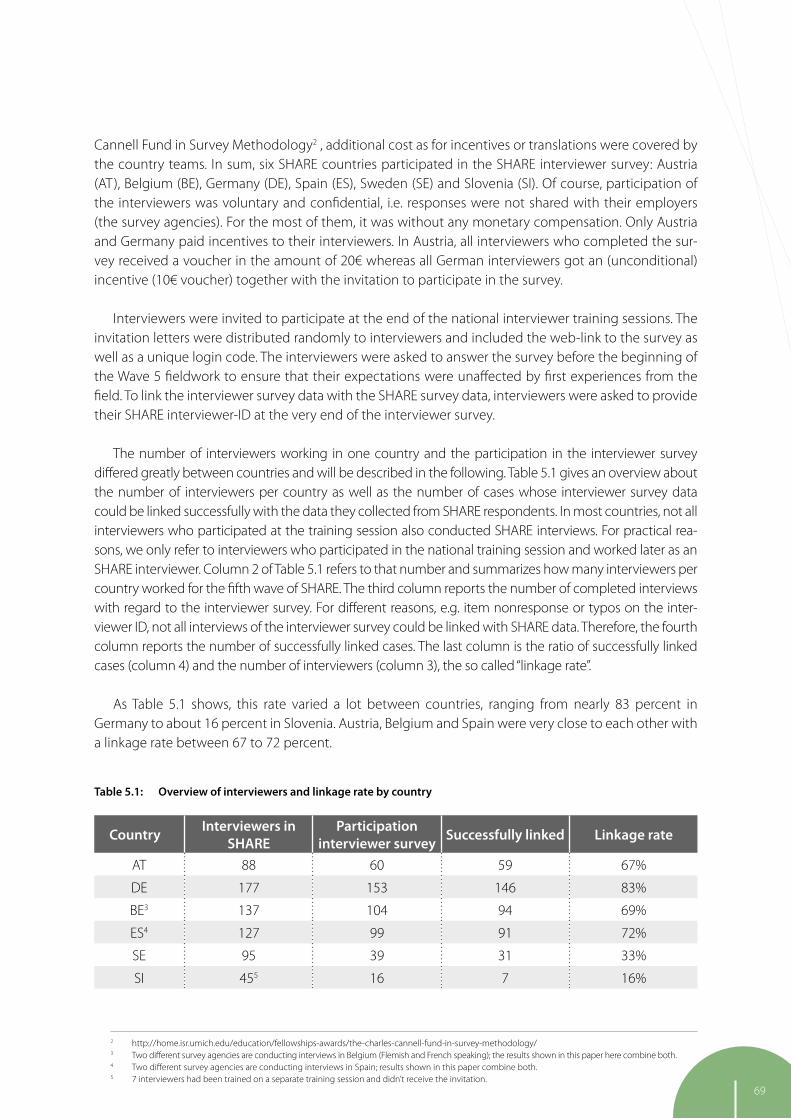
69
Cannell Fund in Survey Methodology2 , additional cost as for incentives or translations were covered by the country teams. In sum, six SHARE countries participated in the SHARE interviewer survey: Austria (AT), Belgium (BE), Germany (DE), Spain (ES), Sweden (SE) and Slovenia (SI). Of course, participation of the interviewers was voluntary and confidential, i.e. responses were not shared with their employers (the survey agencies). For the most of them, it was without any monetary compensation. Only Austria and Germany paid incentives to their interviewers. In Austria, all interviewers who completed the sur-vey received a voucher in the amount of 20€ whereas all German interviewers got an (unconditional) incentive (10€ voucher) together with the invitation to participate in the survey.
Interviewers were invited to participate at the end of the national interviewer training sessions. The invitation letters were distributed randomly to interviewers and included the web-link to the survey as well as a unique login code. The interviewers were asked to answer the survey before the beginning of the Wave 5 fieldwork to ensure that their expectations were unaffected by first experiences from the field. To link the interviewer survey data with the SHARE survey data, interviewers were asked to provide their SHARE interviewer-ID at the very end of the interviewer survey.
The number of interviewers working in one country and the participation in the interviewer survey differed greatly between countries and will be described in the following. Table 5.1 gives an overview about the number of interviewers per country as well as the number of cases whose interviewer survey data could be linked successfully with the data they collected from SHARE respondents. In most countries, not all interviewers who participated at the training session also conducted SHARE interviews. For practical rea-sons, we only refer to interviewers who participated in the national training session and worked later as an SHARE interviewer. Column 2 of Table 5.1 refers to that number and summarizes how many interviewers per country worked for the fifth wave of SHARE. The third column reports the number of completed interviews with regard to the interviewer survey. For different reasons, e.g. item nonresponse or typos on the inter-viewer ID, not all interviews of the interviewer survey could be linked with SHARE data. Therefore, the fourth column reports the number of successfully linked cases. The last column is the ratio of successfully linked cases (column 4) and the number of interviewers (column 3), the so called “linkage rate”.
As Table 5.1 shows, this rate varied a lot between countries, ranging from nearly 83 percent in Germany to about 16 percent in Slovenia. Austria, Belgium and Spain were very close to each other with a linkage rate between 67 to 72 percent.
2 http://home.isr.umich.edu/education/fellowships-awards/the-charles-cannell-fund-in-survey-methodology/3 Two different survey agencies are conducting interviews in Belgium (Flemish and French speaking); the results shown in this paper here combine both. 4 Two different survey agencies are conducting interviews in Spain; results shown in this paper combine both. 5 7 interviewers had been trained on a separate training session and didn’t receive the invitation.
Table 5.1: Overview of interviewers and linkage rate by country
CountryInterviewers in
SHAREParticipation
interviewer surveySuccessfully linked Linkage rate
AT 88 60 59 67%
DE 177 153 146 83%
BE3 137 104 94 69%
ES4 127 99 91 72%
SE 95 39 31 33%
SI 455 16 7 16%

70
5.4 First results: Comparisons of characteristics of the interviewers within and between countries
Only if interviewers differ in certain characteristics, these characteristics can be used to explain inter-viewer effects. The following figures show that there is considerable variation in key variables between interviewers and also between countries. Slovenian interviewers are not considered in the following as the analysis would be based on seven interviews only. The first two figures show the variation in inter-viewers’ gender and age.
Figure 5.2: Gender of the interviewers by country
AT
0%
20%
40%
60%
80%
100%
DE ES BE SE
Gender
Female
Male
In all countries, except in Germany, the majority of interviewers were female ranging from 77 percent in Sweden to 64 percent in Austria. Only in Germany, male interviewers dominate with 59 percent. Even more obvious were the differences in interviewers’ age. Figure 5.3 shows the distribution of interviewers’ age using box-plots. The horizontal line within the box refers to the median age in each country. The red line in the graph marks the age 50 (the age at which people get age-eligible for SHARE). The SHARE guidelines suggested selecting interviewers which were in the same age span as their respondents. The German and Swedish survey agency seemed to follow these suggestions best. These interviewers were older than those of other countries and with a smaller variation.

71
Previous research has shown that interviewers’ experience is an important determinant of inter-viewer effects (e.g. Korbmacher, 2014; Durrant et al., 2010). When considering the average number of years interviewers worked in their job, the countries didn’t differ by much. The average varied between 8 and 11 years. Nevertheless, a more detailed examination of the interviewers’ experience showed that the distributions of the interviewers’ experience varied more than the mean alone would be able to tell. Figure 5.4 displays the job experience of the interviewers broken down into four categories6 .
AT DE ES BE SE
Interviewers´ Experience
first year
70%
60%
50%
40%
30%
20%
10%
0%
1-10 years
11-20 years
over 20 years
Figure 5.4: Experience of the interviewers by country
6 Based on question v1: „In what year did you first start working as an interviewer?” it has to be kept in mind that the timespan must not indicate continuous tenure as interviewer.
Figure 5.3: Age of the interviewers by country
20
30
40
50
60
70
80
AT DE ES
Age
BE SE

72
The most obvious dissimilarities could be found with regard to interviewers with less than one year of experience. In Germany and Spain, none of the interviewers worked in their job for less than one year whereas Belgium and Sweden showed a considerable amount of interviewers with less than one year of job experience.
The last two figures refer to the interviewers’ attitudes towards reluctant respondents. In the ques-tionnaire we gave a list of eight statements on how interviewers could engage with reluctant respond-ents. The two statements we selected here refer to a normative belief about whether or not reluctant respondents should be persuaded to participate and to self-efficacy, i.e. whether or not the participa-tion of reluctant respondents was under the control of the interviewer. Response options were “strongly agree”, “somewhat agree”, “somewhat disagree” or “strongly disagree”. We combined the first two answers into agree. The share of interviewers who agreed to the statement that “Reluctant respondents should always be persuaded to participate” and “With enough effort, even the most reluctant respondent can be persuaded to participate” is illustrated in Figure 5.5 and 5.6, respectively.
0%
20%
40%
60%
80%
100%
AT BE DE ES SE
Reluctant respondents should always be persuaded to participate
Figure 5.5: Percentage of agreement towards reluctant respondents by country

73
A comparison of the two statements shows that agreement was higher for the first statement com-pared to the second across all countries. So the majority of all interviewers confirmed that it is important to persuade reluctant respondents, but only in Spain and Sweden the majority of interviewers also assumed that it was matter of interviewers’ effort.
5.5 Conclusion
Interviewers are an important actor within the process of conducting a survey. They have a high po-tential to influence different survey outcomes. The descriptive analysis of aspects prone to interviewer effects is an important first step. Understanding the mechanisms behind these effects is the logical next step. Our interviewer survey carries high potential for analyzing and understanding the effect of the interviewer within the Survey of Health, Aging and Retirement in Europe. The descriptive comparison of interviewer characteristics shows that there is variation between interviewers within one country and also between countries. This is an important prerequisite to identify characteristics of the interview-ers which can explain interviewer effects. At the time of writing, the data of the interviewer survey is slated for released together with the first release of the Wave 5 SHARE data in March 2015. Information on how to get access to the data will be made available on the SHARE home page: http://www.share- project.org/methodological-research/interviewer-survey.html
We plan to extend this project to additional waves of SHARE as well as to additional SHARE countries. The survey will be implemented in SHARE’s sixth wave in up to 11 countries. To increase the response rates, in-centives will be paid to all interviewers who will complete the survey. As some countries will participate for the second time, with the beginning of Wave 6, the interviewer survey also starts its longitudinal dimension.
0%
20%
40%
60%
80%
100%
AT BE DE ES SE
With enough effort, even the most reluctant respondent can be persuaded to participate
Figure 5.6: Percentage of agreement towards reluctant respondents by country

74
ReferencesBlohm, M., Hox, J. & Koch, A. (2006). The influence of interviewers’ contact behavior on the contact and cooperation rate in face-to-face household surveys. International Journal of Public Opinion Research. 19(1), pp. 97-111.
Blom, A.G., de Leeuw E.D. & Hox, J. (2011). Interviewer effects on nonresponse in the European Social Survey. Journal of Official Statistics. 27(2), pp. 359-377.
Blom, A.G. & Korbmacher, J.M. (2013). Measuring interviewer characteristics pertinent to social surveys: a conceptual framework. Survey Methods: Insights from the Field. Retrieved from: http://surveyinsights.org/?p=817.
Campanelli, P. & O’Muircheartaigh, C. (1999). Interviewers, interviewer continuity, and panel survey non-response. Quality and Quantity. 33(1), pp. 59-76.
Durrant, G.B., Groves, R.M., Staetsky, L. & Steele, F. (2010). Effects of interviewer attitudes and behaviors on refusal in household surveys. Public Opinion Quarterly. 74(1), pp. 1-36.
Groves, R.M. & Couper, M.P. (1998). Nonresponse in household interview surveys. New York: Wiley Series in Probability and Statistics.
Groves, R. M., Fowler, F. J., Couper, M. P., Lepkowski, J. M., Singer, E. & Tourangeau, R. (2009). Survey me-thodology. Hoboken, New Jersey: Wiley Series in Survey Methodology.
Korbmacher, J. (2014). Interviewer effects on respondents’ willingness to provide blood samples in SHARE. SHARE Working Paper Series 20-2014, Munich: Munich Center for the Economics of Aging (MEA).
Lipps, O. & Pollien, A. (2011). Effects of interviewer experience on components of nonresponse in the European Social Survey. Field Methods. 23(2), pp. 156-172.
Pickery, J. & Loosveldt, G. (2001). An exploration of questions characteristics that mediate interviewer effects on item nonresponse. Journal of Official Statistics. 17(3), pp. 337-350.
Pickery, J. & Loosveldt, G. (2002). A multilevel analysis of interviewer effects on various components of unit nonresponse. Quality and Quantity. 36(4), pp. 427-437.
Schaeffer, N.C., Dykema, J. & Maynard, D.W. (2010). Interviewers and interviewing. In: Marsden, P.V. & Wright J.D. (Eds.) 2010. Handbook of Survey Research, pp. 437-470. Bingley UK: Emerald.
Singer, E., Frankel, M.R. & Glassman, M.B. (1983). The effect of interviewer characteristics and expecta-tions on response. Public Opinion Quarterly. 47(1), pp. 68-83.

75
6 Sample design and weighting strategies in SHARE Wave 5Giuseppe De Luca,University of PalermoClaudio Rossetti, LUISS Guido CarliFrederic Malter, Munich Center for the Economics of Aging (MEA) at the Max Planck Institute for Social Law and Social Policy (MPISOC)
6.1 Introduction
This chapter provides a description of the sampling design and weighting strategies adopted in the fifth wave of SHARE. We begin by defining the target population that SHARE aims to represent (6.2). Next, we describe the sampling design focusing on the basic principles guiding the construction of the SHARE sample (6.3), the role played by sampling frames for coverage of the target population (6.4), and other important aspects of sampling - such as stratification, clustering and variation in selection probabilities - that affect the efficiency of sample-based inference (6.5). The chapter concludes with a description of the weighting strategies adopted by SHARE to handle problems of unit nonresponse in the baseline and refreshment samples and problems of attrition in the panel sample (6.6).
6.2 What population does SHARE represent?
In principle, the target population for inference from SHARE is the European population aged 50 and older at a particular point in time. In practice, however, the population that SHARE can represent at each wave differs from this theoretical target because of practical obstacles related to country coverage, sampling and data collection.
Figure 6.1: Country coverage in the fifth wave of SHARE

76
First, SHARE does not include all European countries. As illustrated in Figure 6.1, the fifth wave of this longitudinal survey covered 14 European countries. Of these, 13 countries (Austria, Belgium, Czech Republic, Denmark, Estonia, France, Germany, Italy, Netherland, Slovenia, Spain, Sweden and Switzer-land) had participated in at least one of the previous waves and one country (Luxemburg) was entering SHARE in the fifth wave. Five European countries (Greece, Hungary, Ireland, Poland and Portugal) had participated in one of the previous waves, but they did not participate in Wave 5. In addition, the fifth wave of SHARE also included one non-European country (Israel).
Second, the target population of SHARE does not include people who did not speak (one of ) the official national language(s) of the country1, and people who were either incarcerated, hospitalized, or out of the country during the entire fieldwork period. People who were residents in nursing homes and other institutions for elderly were considered to be part of the target population investigated by SHARE, but as discussed later in Section 6.4 this population group may not be well represented in all countries due to the lack of suitable sampling frames.
Third, as the household level was important for most of the variables collected in SHARE, the spouses/partners of people aged 50 and older were included in the target population regardless of their own age.
Thus, in the countries participating in the fifth wave of SHARE, the definition of the target population was:
Persons born in 1962 or earlier, and persons who are a spouse/partner of a person born in 1962 or earlier, who speak (one of) the official language(s) of the country (regardless of nationality and citizen-ship) and who do not live either abroad or in institutions such as prisons and hospitals during the entire fieldwork period.
The target population of SHARE could also be defined in terms of households. This was implicitly defined as all households with at least one member belonging to the target population of individuals.
6.3 The basic principle of the SHARE sampling design
The rationale for SHARE sample is the same that all advanced population-based survey programs apply at present. Kish (1994, p.173) provided the underlying idea:
“Sample designs may be chosen flexibly and there is no need for similarity of sample designs. Flexibility of choice is particularly advisable for multinational comparisons, because the sampling resources differ greatly between countries. All this flexibility assumes probability selection methods: known probabilities of selection for all population elements.”
In order to facilitate inference to the population of interest, the survey must be based upon probability samples with full population coverage. This was the key principle of the SHARE sampling design in Wave 5. The availability of a probability sample ensures that every unit in the target population has a chance greater than zero of being selected into the sample. Further, it should be possible to compute the selection proba-bility of each individual to enable valid inference on the target population using (weighted) sample statistics.
1 For countries with more than one national language SHARE uses a language-specific CAPI interview. This was the case in Belgium, Switerland, Estonia, Israel, Luxembourg and Spain.

77
6.4 Sampling frames and coverage errors
In general, finding the most suitable sampling frame (i.e. an updated list of the population units) is a very difficult, challenging and time consuming step of all cross-national surveys. Under-coverage and over-coverage errors in the sampling frame may in fact introduce non-sampling errors which may jeop-ardize the standard properties of sample-based inference. SHARE was no exception to this rule.
Since a common sampling frame for all countries was not available, the extent to which full coverage of the target population could be achieved depended crucially on the quality of the sampling frame available in each country. As in the previous waves, the sampling frame and the associated sampling de-sign were not restricted to be the same in all countries, but the basic principles of probability sampling with minimal coverage errors guided the choice of the national sampling designs. For similar reasons, country teams were not forced to use the sampling frame and sampling design used in the previous waves. As a general rule, countries are allowed to use the best sampling frame available at each wave.
For the target population of SHARE, a key feature any “candidate frame” had to fulfill was the avail-ability of reliable information on age. If this information was not available from a given sampling frame, a preliminary screening procedure had to be applied before starting the fieldwork. The table below summarizes the national sampling frames used in Wave 5.
Country Description of frame Units
Belgium National population register I
Czech Republic Listing of dwellings A
Denmark National population register I
Spain (Province of Girona) Municipal population registries I
Germany Municipal population registries I
Israel National population register I
Italy Municipal electoral registries I
Luxemburg National population register (Social security admin.) I
Netherlands Municipal population registries I
Slovenia National population register I
Sweden National population register (Swedish tax authority) I
Table 6.1: Description of sampling frames in countries with baseline/refreshment samples in Wave 5
Due to privacy or legal restrictions it was not always possible to use the best existing frame in a given country. For example, Austria has a modern, computer-based population register. But this register was and still is (as of spring 2015) unfortunately not accessible for survey sampling. On the other hand, SHARE was the first survey that was allowed to use the Swiss population register, which is known to be of excellent quality.
A-Addresses, I-Individuals

78
To our knowledge, some under-coverage error may have occurred for residents of nursing homes and other institutions for elderly. Three countries (Belgium, Czech Republic, and Italy) told us that their frame would exclude residents of nursing homes, thus the resulting net sample would include only resi-dents of private households. A first glance at the data revealed that residents of nursing homes may be present in these country samples of the fifth wave despite their presumable exclusion in the sampling frame. This could have happened due to a number of reasons: they were either wrongly recorded in the sampling frame as private households or interviewers mis-operated the interviewing software (i.e. checked “nursing home” instead of “private household”).Of course, the simple availability of these few sample observations does not ensure a good representation of this important segment of the target population as the process by which these respondents become part of the sample will remain unclear. In principal, coverage of people who were residents of nursing homes was possible only in countries that did not systematically exclude residents of nursing homes from their sample frame (Germany, Den-mark, Israel, Luxemburg, The Netherlands, Sweden and Slovenia). These country-specific coverage errors may play an important role for inference on particular population groups such as the oldest-old. The national sampling frames of some countries were also subject to other minor forms of under-coverage due to outdate information on addresses (Belgium and Italy), or the exclusion of non-citizens (Italy), or lack of individual consent to take part in sample surveys (Denmark), or lack of cooperation from munici-palities supposed to deliver parts of the country sample (Netherlands).
6.5 Sampling designs
After choosing the best sampling frame available in each country, the next step was the selection of a particular design for the national sampling schemes (i.e. the procedures to draw the national samples from the national sampling frames). Under the ideal conditions of full response and full population cov-erage, probability sampling ensures that a sample can provide unbiased estimates of the population parameters of interest. However, several features of the sampling design may have still affected preci-sion of the estimates. For this reason, a number of advices on stratification, clustering, variation in selec-tion probabilities and sample size were provided to all participating countries by means of the “SHARE Sampling Guide” and bilateral discussion with the SHARE Central Coordination team. These important aspects of the sampling design are summarized in the following subsections.
6.5.1 Stratification
Regional stratification schemes were particularly recommended in order to ensure a good repre-sentation of different geographical areas within the country, improve efficiency of the survey estimates and reduce the costs of the interview process. If other relevant characteristics were available from the sampling frame – such as age and gender in the case of population registers – countries were advised to also use them for stratification.

79
6.5.2 Clustering and variation in inclusion probabilities
As in other surveys, such as the European Social Survey (ESS) or the Programme for the International Assessment of Adult Competencies (PIAAC), another guiding principle of SHARE was the design of sam-pling schemes which yield a minimum variation of inclusion probabilities and a minimum amount of clustering. However, the design of sampling schemes with such characteristics was not always possible due to the lack of suitable sampling frames.
Such a scenario applied, for example, if a country team only had access to a list of households and an eligible person has to be selected from all eligible target persons of a sampled household. In this case, variation in inclusion probabilities cannot be avoided and the national sampling scheme necessarily introduced a so-called “design effect due to unequal inclusion probabilities”
where n is the sample size and 𝑤𝑖 are design weights defined as the inverse of the inclusion probabilities.
Other studies (e.g. ESS) have shown that 𝐷𝑒𝑓𝑓𝑝 usually ranges between 1.20 and 1.25 for designs that involve the random selection of one adult per household, depending on the variation of household sizes in a country. This variation in inclusion probabilities had to be taken into account by a design weight which was the inverse of the inclusion probability. For SHARE, 𝐷𝑒𝑓𝑓𝑝 was smaller than this, as it depended on the distribution of the number of age-eligible units per household, rather than the total number of adults per household, where an age-eligible unit is defined as either a single person aged 50 or over or a couple containing at least one person aged 50 or over. In most countries, most households did not contain more than one age-eligible unit and very few had more than two.
Fortunately, some countries (Denmark, Slovenia, Switzerland and Germany) had access to popula-tion registers and sample schemes which yielded equal inclusion probabilities for all elements could therefore be implemented. In Germany, however, SHARE had to use a two-stage clustered sampling scheme as the population registers were locally administered by the municipalities. A number of mu-nicipalities had to be selected at the first stage and age eligible persons at the second stage. In such a case, an additional component of the design effect emerges. It is the design effect due to clustering defined as the ratio of the variance of a given clustered sample’s estimate to the variance of the estimate under simple random sampling
where θ denotes an estimate under consideration, is the variance of the estimate under cluster sampling, and is the variance of the estimate under simple random sampling. A value of the design effect of, say 2, means that the sample variance is two times bigger than it would be if the survey were selected randomly with the same sample size. Depending on the degree of homo-geneity in the data, the design effect due to clustering usually ranges from 1 to 3 since both the mean cluster size of the primary sampling units (municipalities, in the case of Germany) and the intraclass correlation determine its magnitude. Therefore, by design, the mean cluster size had to be chosen as small as possible and as many primary sampling units as possible had to be selected. Of course, this was at odds with the interests of survey agencies for which an increase in the number of primary sampling units was often associated with higher survey costs.

80
6.5.3 Composition and size of the SHARE sample
Sample composition and size of the national samples are two additional features of the samp-ling design affecting efficiency of cross-sectional and longitudinal analyses. Table 6.2 below gives an overview of all countries that ever participated in SHARE and the composition of their samples in the respective wave(s).
CountryWave 1 Wave 2 Wave 3 Wave 4 Wave 5Baseline Panel Refresh. Baseline Panel Panel Refresh. Baseline Panel Refresh. Baseline
AT BE_FR BE_NL
CH CZ DE DK EE ES FR GR HU IL IT LU NL PL PT SE SI
Table 6.2: Sample type by wave and country
Luxemburg, which entered SHARE for the first time in Wave 5, had to construct its baseline sample that would ultimately form the “first wave” panel sample for the next waves of the study. For all other countries which had participated in any of the previous four waves conducted so far, no panel rotation method was used in order to maximize the sample size available for longitudinal analyses. In other words, all units in the panel sample were considered eligible for the interview of the fifth wave, inclu-ding the non-responding partners of peoples who were interviewed in some previous wave.
As can be seen in the table above, many longitudinal countries also had a refreshment sample in
Wave 5. The aim of these refreshment samples was twofold: i) achieve representation of the younger age-cohort of the target population of Wave 5 (i.e. people born between 1960 and 1962) that were not age-eligible in the previous waves, and ii) compensate the reduction in the size of the panel sample due to attrition.

81
The choice of conducting a refreshment sample was so far up to the country, because all countries had to apply for their own funding to their national funding agencies. Several countries had to select refreshment samples of people born between 1961 and 1962 to add to their existing sample of people born in 1960 or earlier.2 The Wave 5 refreshment samples of Germany, Israel and Sweden included peo-ple born between 1957 and 1962 to compensate the lack of a refreshment sample in Wave 4. Additio-nally, many countries deemed it necessary to implement a refreshment sample across the full age range of people born in 1962 or earlier to compensate the effect of panel attrition on all age-cohort. Where possible, these full-range refreshment samples included an over-sampling of persons born in 1961 and 1962 (or 1957 to 1962 if the country had no Wave 4 refreshment sample) to maintain the representation of the younger age-cohorts.
SHARE did not define a minimum net sample size (like for example PIAAC does) because of the fol-lowing reasons:
• The attrition rate of the longitudinal sample was difficult to estimate in advance. • In countries where no a-priori information on age eligibility from the frame was available
(e.g. the Czech Republic), a screening procedure had to be conducted and the response rate of these contact persons was difficult to anticipate. • The ineligibility rate due to other types of over-coverage errors (e.g. adresses of office building and
farms) had to be estimated in advance. • The response rate of both the selected persons in the refreshment sample and their partners/
spouses was also difficult to estimate in advance. Moreover, whether there was a partner/spouse to be interviewed was not known from the sampling frames.
Thus, any estimation in advance of the net sample size that would result from any given gross sam-ple size was subject to substantial uncertainty (especially in countries without a frame of individuals) as it relied on several more or less weak assumptions. Useful information on these aspects of the sampling design could be desumed from previous waves, but this was subject to a large amount of variability across both countries and waves. For all these reasons, countries were simply advised to maximize their net sample sizes with the available budget.
6.6 Corrections for nonresponse and sample attrition
Sampling design weights, defined as the inverse of the probability of being included in the sample of any specific wave, allow compensating for unequal selection probabilities of the sample units. In SHARE the probability of including any eligible household member is equal to the probability of inclu-ding the household. Thus, selection probabilities and sampling design weights are the same for the household and for any eligible household member.
Under the ideal situation of complete response, these weights allow to obtain unbiased estimators of the population parameters of interest. Unfortunately, survey data are always affected by unit nonrespon-se (i.e. eligible sample units fail to participate in the survey because of either noncontact or explicit refu-sal to cooperate) and respondents in a given wave of a panel study may also drop out in a subsequent
2 Wave 1 baseline samples consisted of people born in 1954 or earlier. The refreshment samples in waves 2 and 4 contained, respectively, people born between 1955 and 1956 and people born between 1957 and 1960. No refreshment samples were added in Wave 3.

82
wave generating attrition in the longitudinal sample. So, estimators constructed on the basis of sample design weights alone may be biased because they ignore possible selection effects due to these types of nonsampling errors (Lessler and Kalsbeek, 1992). Although sample design weights will be included in the public release of the SHARE data, users of the SHARE data are not recommended to rely on these weights alone unless they are used for the implementation of other nonresponse correction methods.
The strategy used by SHARE to cope with selection effects induced by unit nonresponse and panel attrition relies on the ex-post calibration procedure proposed by Deville and Särndal (1992).3 As dis-cussed in De Luca and Rossetti (2008), this statistical re-weighting procedure gives calibrated weights which are as close as possible, according to a given distance measure, to the original design weights while simultaneously respecting a set of known population totals (the calibration margins). Under cer-tain assumptions on the missing data process, calibrated weights may help to reduce the selection bias generated by unit nonresponse and panel attrition. The key assumption was that the key survey variab-les are independent of the missing data process conditional on the available set of calibration variables. In the terminology of Rubin (1987) this corresponded to assuming that the process generating missing observations was missing-at-random (MAR). This assumption could be relaxed by considering more sophisticated approaches where the process for the outcome of interest and the response process were estimated jointly (see, for example, De Luca and Peracchi, 2012). However, these model-based approa-ches were specific to the research questions under investigation. Moreover, instead of requiring auxili-ary information on the subset of responding sample units and the corresponding calibration margins in the target population, they required information on all eligible sample units (both respondents and nonrespondents). Thus, depending on the purpose of the analysis to be performed, users should decide whether the SHARE calibrated weights will be appropriate to compensate for the potential selection bias due to unit nonresponse and panel attrition.
As in previous waves, the public release of the Wave 5 data will include calibrated cross-sectional weights and calibrated longitudinal weights, which were designed for cross-sectional and longitudinal analyses, respectively. Further, since the basic units of analysis can be either individuals or households, both types of weights were computed at the individual level for inference to the target population of individuals and at the household level for inference to the target population of households. Additional information on these different types of weights is provided in the following subsections.
6.6.1 Calibrated cross-sectional weights
Calibrated cross-sectional weights were defined for the sample of 50+ respondents, either individu-als or households, in Wave 5 pooling longitudinal and refreshment samples. Since the basic units of analysis can be either individuals or households, SHARE provides two sets of calibrated weights: one at the individual level and one at the household level. At the individual level, each 50+ respondent received a calibrated weight that depended on the household design weight and the respondent‘s set of calibration variables. At the household level, each interviewed household member received an iden-tical calibrated weight that depended on the household design weight and the calibration variables of all 50+ respondents in that household. Calibrated weights were computed separately by country to match the size of national populations of individuals born in 1962 or earlier. Within each country, we
3 Of course, other approaches to handle problems of unit nonresponse and attrition are possible. Since many of the underlying assumptions are untestable, we always encourage data users to compare the outcomes from alternative approaches to investigate robustness of their findings.
83
used a set of calibration margins for the size of the target population across 8 gender-age groups (i.e. males and females with year of birth in the classes (-1932], [1933-42], [1943-52], [1953-62]) and across NUTS1 regional areas. The source of these population totals was Eurostat. Table 6.3 shows the calibration margins of population totals across the eight gender-age groups for each country4. Calibrated weights were missing for respondents younger than 50 years (i.e. age-ineligible partners of an age-eligible res-pondent), those with missing information on any variable of the set of calibration variables (i.e. year of birth, gender and NUTS1 code), and those with missing sampling design weights (i.e., respondents with missing sampling frame information).
6.6.2 Calibrated longitudinal weights
Calibrated longitudinal weights differed from calibrated cross-sectional weights in three important respects. First, these weights were only defined for the balanced sample of respondents in at least two waves of the panel. Second, calibrated longitudinal weights took into account mortality of the original target population across waves. Mortality affects both the sample and the population. Thus, the target population for longitudinal analyses was the original population at the beginning of the time refer-ence period that survives up to the end of the period. Third, since the SHARE panel now consisted of five waves, one could compute different types of calibrated longitudinal weights depending on the
4 For brevity we did not report the calibration margins across NUTS1 regional areas. As discussed below, tis information can be found in the supplementary material provided by SHARE for the construction of calibrated weights.
Country Men Women Total(-1932] [1933-42] [1943-52] [1953-62]) (-1932] [1933-42] [1943-52] [1953-62])
AT 141,046 309,215 422,006 590,010 281,321 383,148 463,298 599,021 3,189,065
BE 205,292 365,832 588,818 763,525 381,802 451,293 618,831 764,197 4,139,590
CH 139,023 265,693 429,528 561,013 251,640 322,097 448,861 551,105 2,968,960
CZ 131,288 302,050 640,842 678,641 274,893 423,518 730,174 686,559 3,867,965
DE 1,537,207 3,876,835 4,401,202 6,156,469 2,927,387 4,668,244 4,652,554 6,102,406 34,322,304
DK 85,286 193,604 341,978 364,797 147,397 221,479 351,538 362,954 2,069,033
EE 15,381 39,621 59,507 84,374 47,312 75,360 83,092 97,108 501,755
ES 925,955 1,536,695 2,293,706 3,011,976 1,627,485 1,903,050 2,477,475 3,067,926 16,844,268
FR 1,275,434 2,036,474 3,512,835 4,160,065 2,423,010 2,563,478 3,822,313 4,382,959 24,176,568
IT 1,314,944 2,513,433 3,308,942 3,935,470 2,441,953 3,102,748 3,605,006 4,146,533 24,369,029
LU 7,387 14,643 24,362 36,667 13,655 17,922 24,180 35,025 173,841
NL 247,502 549,443 993,467 1,178,148 455,318 630,268 1,000,144 1,171,940 6,226,230
SE 187,029 347,673 586,249 587,275 311,119 386,531 593,249 577,619 3,576,744
SI 27,493 69,007 112,050 155,322 65,362 94,048 118,608 150,134 792,024
IL 87,930 152,950 290,270 369,220 136,920 192,280 323,120 397,290 1,949,980
Table 6.3: Callibration margins of population totals across gender-age groups by country

84
selected combination of the waves and the basic unit of analysis (either individuals or households). To simplify the structure of the public release of the data, we provided calibrated longitudinal weights only for the balanced panel sample of the last two waves (i.e. the sample of 50+ respondents of Wave 4 and Wave 5). These calibrated weights were computed separately by country to match the size of the national populations of individuals born in 1960 or earlier (i.e. the target population of Wave 4) that survived up to 2012. We used a set of calibration margins for the size of the target population across eight gender-age groups (i.e. males and females with year of birth in the classes (-1930], [1931-40], [1941-50], [1951-60]) and across NUTS1 regional areas (again with the exception of Israel, where we used gender-age groups and the three population subgroups listed above). Mortality was accounted for by subtracting from each population margin the number of deaths between 2010 and 2012. Cali-brated longitudinal weights were available at the individual and the household level. Notice that, for the weights at the household level, we only require that there was at least one eligible respondent in each wave of the selected wave combination. Thus, households with one partner participating in Wave 4 and the other partner participating in Wave 5 belonged to the balanced sample of households for the wave combination 4-5, even if neither partner belonged to the corresponding balanced panel of individuals.
For longitudinal analyses based on other possible combinations of waves, users will be required to compute their own calibrated longitudinal weights. To support users in this methodological task, SHARE provided a Stata command called “cweight.ado” which implemented the calibration procedure by Deville and Särndal (1992), a Stata do-file called “weighting.do” which illustrated step-by-step how to compute calibrated longitudinal weights at the individual and the household level, and tables of coun-try specific information needed to compute the population calibration margins.
ReferencesDe Luca, G. & Peracchi, F. (2012). Estimating engel curves under unit and item non-response. Journal of Applied Econometrics. 27, pp. 1076-1099.
De Luca, G. & Rossetti, C. (2008). Sampling design and weighting strategies in the second wave of SHARE, in Axel Börsch-Supan et al. (Eds.). First Results from the Survey of Health, Ageing and Retirement in Euro-pe (2004-2007) - Starting the Longitudinal Dimension, Mannheim: MEA, pp. 333-338.
Deville, J.C. & Särndal, C.E. (1992). Calibration estimators in survey sampling. Journal of the American Statistical Association. 87(418), pp. 376-382.
Kish, L. (1994). Multipopulation survey designs. International Statistical Review. 62, pp. 167-186.
Lessler, J. & Kalsbeek, W. (1992). Nonsampling error in survey. New York: John Wiley & Sons.
Rubin, D.B. (1987). Multiple imputation for nonresponse in surveys. New York: Wiley.

85
7 Item nonresponse and imputation strategies in SHARE Wave 5Giuseppe De Luca, University of PalermoMartina Celidoni, University of PaduaElisabetta Trevisan, University of Padua & Netspar
7.1 Introduction
Nonresponse is a serious problem that affects most empirical studies based on survey data. A dis-tinction is usually made between two types of nonresponse. The first – unit nonresponse – occurs when eligible sample units fail to participate in a survey because of noncontact or explicit refusal to cooperate (see Chapter 8). The second – item nonresponse – emerges when responding units do not provide useful answers to particular items of the questionnaire as it is often the case with income, wealth and consumption expenditure items. The potential implications of the two types of nonresponse are similar, namely selectivity bias and loss of precision. The key difference is that for unit nonresponse all items of the questionnaire are missing, while for item nonresponse missing observations are confined to specific items of the questionnaire. Such distinction has therefore relevant implications for the auxiliary informa-tion that can be used in ex-post adjustment procedures. For unit nonresponse, the auxiliary informa-tion is necessarily confined to that obtained from the sampling frame or the data collection process (in SHARE, that’s age, gender and regional NUTS1 indicators), whereas for item nonresponse the additional information collected during the entire interview process can be used.
This chapter focuses on item nonresponse in the fifth wave of SHARE and the imputation strategies adopted to fill-in the missing values. The main features of the SHARE interviews and the prevalence of missing data are briefly discussed in Sections 7.2 and 7.3, respectively. In Section 7.4, we describe the strategies adopted to handle some practical issues faced in the construction of the imputation data-base. A non-technical description of the imputation procedure used in Wave 5 is given in Section 7.5. Except for minor differences in the underlying raw data, this procedure is very close to that used for Re-lease 1.1 of Wave 4 data (publicly available since March 2013). Both procedures present however some important innovations with respect to the imputation strategies exploited for Release 2.4 of Wave 1 and Wave 2 data (publicly available since March 2011, see Christelis, 2011). Harmonized imputations for all waves of SHARE are planned to be delivered in the near future.
7.2 Features of the SHARE interview in Wave 5
The way the data are collected and the complexity of the questionnaire are known to be key deter-minants of non-sampling errors such as unit and item nonresponse and measurement errors. The data collection mode adopted in SHARE is the Computer Assisted Personal Interview (CAPI).
To reduce the burden of the interview process, some modules were asked to only one person per household. The so-called family respondent answered questions about children and help received (CH module and part of the SP module). Questions about financial items, total household income, incomes of other non eligible household members, housing, and household consumption expenditures (FT, AS,

86
HH, HO and CO modules) were instead answered by the so-called financial respondent. Since the second wave, the CAPI questionnaire also included skip-patterns for time-invariant variables of respondents who have already participated to previous waves. For these respondents, relevant time-invariant variables were directly preloaded in the interview instrument using the information provided in the previous waves.
Two additional dimensions of the complexity of the interview process were question wording and time reference period. Due to the nature of the topics investigated by SHARE, the wording of some questions was necessarily sensitive. Examples include some questions about physical health (“In which organ or part of the body have you had a cancer?”), mental health (“In the last month, have you felt that you would rather be dead?”), or economic issues (“Thinking of your household’s total monthly income, would you say that your household is able to make ends meet...”). Despite the sensitive wording, the fraction of missing values on this type of closed-ended questions was generally low. Large amounts of missing data occurred in-stead for monetary variables such as incomes, assets, and consumption expenditures which were collected through retrospective and open-ended questions that were sensitive and difficult to answer precisely.
The time reference period of monetary variables varied considerably depending on the question being asked. Questions about employment incomes and financial transfers refer to the last calendar year, questions about consumption expenditures refer to a typical month, and questions about assets refer to the current situation at the time of the interview. For questions about pensions, regular transfers, rent payments, and repayments of loans and mortgages, the period covered by a typical payment was asked after asking for the average amount of the last payments.
In case of initial nonresponse to open-ended questions for monetary variables, the respondent was asked a sequence of unfolding-bracket (UB) questions aimed to recover partial information on the missing mo-netary amount. Specifically, the respondent was asked whether the amount was larger than, smaller than, or about equal to three predefined thresholds defined at the country level. The threshold in the first UB question was assigned randomly and the sequence of UB questions either stops or continues with the next threshold depending on the answer given to the previous questions. The information collected through the sequence of UB questions can be an approximate point estimate (i.e. about equal to one of the three thresholds) or an interval estimate. The sequence of UB questions was uninformative only if the respondent did not give a substantial answer (i.e. neither ‘Refuse’ nor ‘Don’t know’) to the first question of the sequence.
7.3 Prevalence of missing data
As in the previous waves, most of the variables collected in the fifth wave of SHARE were only affected by small amounts of missing data (usually lower than 5%). Non-negligible amounts of missing data occurred instead for monetary variables about incomes, assets and consumption expenditures. Figure 7.1 shows the cross-country distribution of the item nonresponse rates for six monetary variables that are generally affected by a large amount of missing data: annual income from employment (EP205), regular payments from public old age pensions (EP078_1), value of the house (HO024), expenditure on food consumed at home (CO002), amount hold in bank accounts (AS003) and liabilities (AS055). For this set of variables, the cross-country ave-rage of item nonresponse ranges between a minimum of 9 percent for regular payments from public old age pensions to a maximum of 36 percent for amount hold in bank accounts. However, item nonresponse seems

87
Figure 7.1: Percentage of missing values for some monetary variables by country
to be country-specific: Denmark and Sweden, for example, show low percentages of missing data for most of the variables considered (usually lower than 10%). In contrast, Spain, Slovenia, Luxemburg and Israel exhibit item nonresponse rates that are considerably higher than the average. There, item nonresponse be-comes particularly worrisome for some wealth components with more than 60 percent of the data missing.
Although questionnaire design and sample management system are standardized across countries in order to ensure an ex-ante harmonization of the national data, this between-country variability in item nonresponse may reflect the impact of other cross-country differences in fieldwork procedures (e.g. reputation and quality of the national survey agencies, experience, education and training of the interviewers) as well as differences in the composition of the national samples and the compliance be-havior of the national target populations towards the survey requests.

88
7.4 Practical decisions about imputations
Handling item nonresponse in a cross-national, multi-disciplinary and longitudinal survey like SHARE is a challenging task that involves many different decisions that have to be balanced against each other. In this section we therefore describe the key steps that were necessary to construct the imputation mo-del. Since many of the practical issues addressed here unavoidably affect the outcomes of this model, we found it important to inform data users of the rational driving the construction of the SHARE public-use imputation dataset.
Dimensionality of imputation model
Due to the large number of variables collected in SHARE Wave 5, the first issue was how to select a feasible subset of core variables that accommodates a wide variety of analyses that data users might want to perform. Preliminary choices regarding the dimensionality of the imputation model are par-ticularly important in the context of multivariate imputation procedures that attempt to preserve the correlation structure of the imputed variables. Unlike univariate imputation procedures, these meth-ods require that multiple variables are imputed simultaneously on the basis of some Markov Chain Monte Carlo (MCMC) technique. The problem is that as the number of variables to be imputed jointly increases, these iterative techniques often require significant effort in programming and fine tuning. A compromise between generality and complexity of the imputation model was therefore needed. Our strategy to deal with this problem was as follows. First, we selected a rather large number of vari-ables expected to be relevant for the key purposes of the survey. Second, to simplify complexity of the imputation model, our multivariate imputation procedure was employed only for a smaller sub-set of variables with relevant fractions of missing data (see Section 7.5). Furthermore, this procedure was restricted to aggregated subsets of income, wealth and consumption expenditure items only.
Data standardization
After selecting a set of core variables to be imputed, we constructed for each of them a binary eligibility indicator which identified those respondents eligible to answer that specific question by ta-king into account possible inconsistencies in the raw data, country-specific deviations from the gene-ric version of the CAPI questionnaire, branching, skip patterns and proxy interviews. For open-ended questions on monetary variables, which are usually preceded by one or more ownership questions, we also constructed a set of binary ownership indicators to identify a subset of eligible respondents with a non-zero monetary amount. Conditional on eligibility and ownership, non-zero values of monetary variables were converted (if needed) in annual Euro amounts to avoid differences in the time reference period of each question and the national currencies of non-Euro countries.
Outliers
We symmetrically trimmed two percent of complete cases from the country-specific distribution of annual Euro amounts to exclude outliers that may have a disproportional influence on survey statistics. This implies that, in addition to non-substantial answers (“Don’t know” and “Refusal”), we also imputed outliers in the tails of the distribution of each monetary variable.

89
Logical constraint
Complete cases and imputed values were required to satisfy a set of logical constraints on owner-ship of the variables included into the imputation model which helped to avoid unreasonable com-binations of the imputed data. For example, the ownership indicators of some financial assets (bonds, stocks and mutual funds) are set to zero (no ownership) if it is known that the household does not own a bank account.
Preserving the partial information from sequences of UB questions
Another useful source of information to reduce uncertainty on missing values of monetary variables is given by the sequence of answering UB questions. Table 7.1 and Table 7.2 show that, in several cases, this survey instrument allows recovering helpful information for more than 50 percent of the initial missing data. As mentioned before, the information derived from UB questions can be of two types: approximate point estimates (1) or interval estimates (2). In the first case, missing amounts are directly imputed using the thresholds selected by the respondents throughout the sequence of UB questions. In the second case, UB interval estimates are combined with the additional information from logical constraints and percentiles of the country distribution to shrink as much as possible the bounds placed on missing data.
CountryIncome
from employment
Publicold age pension
Expenditure on food
consumed at home
Valueof the house
Amount in bank account
Liabilities
Austria 0.21 0.22 0.41 0.33 0.17 0.08
Germany 0.10 0.17 0.36 0.3 0.17 0.09
Sweden 0.21 0.32 0.37 0.13 0.13 0.14
Netherlands 0.19 0.29 0.35 0.21 0.12 0.03
Spain 0.18 0.24 0.37 0.33 0.17 0.16
Italy 0.28 0.19 0.39 0.35 0.25 0.21
France 0.13 0.26 0.43 0.30 0.19 0.14
Denmark 0.14 0.23 0.5 0.14 0.12 0.08
Switzerland 0.19 0.22 0.39 0.24 0.22 0.25
Belgium 0.19 0.17 0.36 0.35 0.12 0.1
Israel 0.08 0.11 0.19 0.09 0.1 0.11
Czech Republic 0.24 0.25 0.37 0.36 0.19 0.15
Luxembourg 0.10 0.06 0.17 0.08 0.11 0.04
Slovenia 0.22 0.12 0.42 0.23 0.14 0.12
Estonia 0.18 0.49 0.35 0.26 0.22 0.19
Total 0.18 0.24 0.37 0.27 0.17 0.13
Table 7.1: Fraction of point estimates provided by the sequences of UB questions as percent of initially missing data

90
CountryIncome
fr om employment
Publicold age pension
Expenditure on food
consumed at home
Valueof the house
Amount in bank account
Liabilities
Austria 0.43 0.32 0.27 0.46 0.37 0.47
Germany 0.50 0.47 0.31 0.40 0.34 0.44
Sweden 0.45 0.36 0.31 0.39 0.33 0.33
Netherlands 0.41 0.39 0.25 0.38 0.27 0.30
Spain 0.24 0.23 0.18 0.29 0.20 0.36
Italy 0.25 0.28 0.23 0.31 0.24 0.27
France 0.55 0.43 0.35 0.46 0.45 0.61
Denmark 0.33 0.23 0.25 0.45 0.27 0.29
Switzerland 0.45 0.23 0.26 0.37 0.29 0.31
Belgium 0.44 0.32 0.38 0.39 0.37 0.49
Israel 0.34 0.31 0.24 0.52 0.29 0.33
Czech Republic 0.35 0.27 0.32 0.29 0.24 0.35
Luxembourg 0.44 0.50 0.53 0.64 0.32 0.31
Slovenia 0.32 0.43 0.19 0.26 0.18 0.20
Estonia 0.43 0.23 0.37 0.34 0.33 0.38
Total 0.39 0.32 0.29 0.38 0.30 0.38
Table 7.2: Fraction of interval estimates provided by the sequences of UB questions as percent of initially missing data
Aggregation
After exploiting the information available for each item, we reduced the number of monetary vari-ables that had to be imputed jointly by aggregating 55 items on income, wealth and consumption expenditure into 17 aggregated variables. Each aggregated variable is obtained by summing two or more original items as illustrated in Table 7.3. Notice that the choice of aggregating such long list of income, wealth and expenditure items into a considerably smaller subset of key variables was consid-ered a reasonable strategy to reduce the computational complexity of the imputation model. However, the use of aggregated variables is not a panacea. This simplification has both theoretical and practical implications. From a theoretical viewpoint, aggregation corresponds to imposing linear restrictions on the imputation model and this may undermine validity of the analyses that users can perform on the basis of imputed data (see, for example, Rubin, 1996). From a practical viewpoint, the SHARE public-use data only contain imputations for the chosen set of aggregated variables, but not for their particular components. In addition, special attention was needed to deal with country-specific deviations from the generic version of the CAPI questionnaire and the preservation of the partial information available for missing aggregated values. The last issue was particularly important because, when aggregating several items, it was often the case that only some of them were missing. Moreover, logical constraints and sequences of UB questions may provide interval information on the missing observations of each item. Thus, even if aggregated variables are regarded as missing, the available information for the single components can be used to define bounds for missing aggregated values.

91
Aggregate variables Components Variablename
Regular payments from public old age, early reti-rement, survivor and war pensions
Public old age pensionPublic old age supplementary pensionPublic early retirement pensionMain public survivor pensionSecondary public survivor pensionPublic war pension
EP078_1EP078_2EP078_3EP078_7EP078_8EP078_9
Regular payments from pri-vate occupational pensions
Occupational old age pension from last jobOccupational old age pension from second jobOccupational old age pension from third jobOccupational early retirement pensionOccupational disability or invalidity insuranceOccupational survivor pension
EP078_11EP078_12EP078_13EP078_14EP078_15EP078_16
Regular payments from disability pensions and benefits
Main public disability insurance pensionSecondary public disability insurance pension
EP078_4EP078_5
Regular payments of other private pensions
Regular life insurance paymentsRegular private annuity or personal pension paymentsLong-term care payments from private insurance
EP094_1EP094_2EP094_5
Regular payments from private transfers
AlimonyRegular payment from charities
EP094_3EP094_4
Lump-sum payments from public old age, early retirement, survivor and war pensions
Lump-sum payments from public old age pensionLump-sum payments from public old age supplementary pensionLump-sum payments from public early retirement pensionLump-sum payments from main public survivor pensionLump-sum payments from secondary public survivor pensionLump-sum payments from public war pension
EP082_1EP082_2
EP082_3
EP082_7EP082_8
EP082_9
Lump-sum payments from private occupational pensions
Lump-sum payments from occupational old age pension from last job Lump-sum payments from occupational old age pension from second jobLump-sum payments from occupational old age pension from third jobLump-sum payments from occupational early retirement pensionLump-sum payments from occupational disability or invalidity insuranceLump-sum payments from occupational survivor pension
EP082_11
EP082_12
EP082_13
EP082_14
EP082_15
EP082_16
Lump-sum payments from disability pensions and benefits
Lump-sum payments from main public disability insurance pensionLump-sum payments from secondary public disability insurance pension
EP082_4EP082_5
Table 7.3: Aggregate variables in Wave 5

92
Table 7.3: Aggregate variables in Wave 5 (continued)
Aggregate variables Components Variable name
Lump-sum payments of other private pensions
Lump-sum payments from life insurance Lump-sum payments from private annuity or personal pension Lump-sum payments from long-term care private insurance
EP209_1EP209_2
EP209_5
Lump-sum payments from private transfers
Lump-sum payments from alimonyLump-sum payments from charities
EP209_3EP209_4
Rent and home-related expenditures
Amount rent paidOther home-related expenditures
HO005HO008
Income from rent or sublet
Income from subletIncome from rent of real estate
HO074HO030
Income from other household members
Other household members’ net incomeOther household members’ net income from other sources
HH002HH011
Bond, stock and mutual funds
Government/corporate bondsStocksMutual funds
AS007AS011AS017
Savings in long term investments
Individual retirement accounts from respondentIndividual retirement accounts from partnerContractual savingsWhole life insurance holdings
AS021AS024AS027AS030
Paid out-of-pocket for outpatient care
Paid out-of-pocket for doctor visitsPaid out-of-pocket for dental care
HC083HC093
Paid out-of-pocket for nursing home and home-based care
Paid out-of-pocket for home-based care Paid out-of-pocket for nursing home
HC129HC097
7.5 The imputation procedure used in SHARE
The imputation procedure used in Wave 4 and Wave 5 exhibited some important innovations with respect to the procedure adopted in Wave 1 and Wave 2. Two differences were particularly striking. First, as discussed in the previous section, some items were now imputed in aggregate terms to simplify the computational burden of the imputation model. For similar reasons, separate imputations for longitudi-nal and refreshment subsamples were no longer considered and lagged variables from previous waves were not used as predetermined predictors any more. The second important difference is that we han-dle the problem of non-responding partners (NRPs) differently, namely the fact that only one of the two partners may have agreed to be interviewed. Unlike the strategy adopted in the first two waves, NRPs are now viewed as a problem of unit nonresponse (not item nonresponse) due to the limited informa-tion available to cope with this type of nonresponse error. Our imputation procedure provides only an indirect estimate of the income from NRPs to avoid understating total household income when only one of the two partners was interviewed. As discussed at length at the end of this section, the strategy used to recover this information exploits the distinction between couples with and without NRPs and additional information obtained from a one shot question on monthly household income (HH017).

93
Similarly to the previous procedure, variables of Wave 5 were imputed by univariate or multivariate methods depending on the prevalence of missing values. Simple univariate methods, such as hot-deck and regression imputations, were used when the fraction of missing values was lower than 5 percent for the entire sample and lower than 10 percent at the country level. Variables with fractions of missing values above these thresholds were instead imputed jointly by the fully conditional specification (FCS) method (van Buuren et al., 1999; Raghunathan et al., 2001), an iterative imputation procedure. More precisely the FCS method imputes multiple variables iteratively via a sequence of univariate imputa-tion models, one for each imputation variable, using as predictors all variables except the one being imputed. Despite a lack of rigorous theoretical justification (see, for example, Arnold et al., 1999, 2001; van Buuren et al. 2006; van Buuren, 2007), the FCS method is one of the most popular multivariate impu-tation procedures used in practice due to its flexibility in handling complicated data structures. Recent comparisons of the FCS method with other multivariate imputation methods can be found in Lee and Carlin (2010) and references therein.
Univariate imputations
This set of imputations was performed in an early stage separately by country. We first imputed socio-demographic characteristics such as age and education that were affected by a small fraction of missing values so that these variables could then be used as exogenously observed predictors in the imputation of the other variables. Our set of predictors for hot-deck imputations typically included gender, age group, years of education and self-reported health. For some variables additional predictors were also used. For example, we also employed the number of children when imputing the number of grandchildren and an indicator for being a patient in a hospital overnight during the last year when im-puting health-related variables. Variables that were known to be logically related, such as respondent’s weight, height and body mass index, were imputed simultaneously by hot-deck.
Multivariate imputations
FCS imputations were performed separately by country and household type to allow for heteroge-neity across these different groups. The household types considered were singles and third respond-ents1 (sample 1), couples with both partners interviewed (sample 2), and all couples – with and without NRPs (sample 3). Notice that sample 2 is embedded into sample 3. This overlapping partitioning of the sample was introduced to estimate total household income in couples with NRPs. The basic idea was that we could first impute total household income of couples belonging to sample 2. In sample 3, couples with both partners interviewed could then be used as valid observations to impute total household income of couples with NRPs. Before providing additional details on this aspect of the new imputation procedure, we discuss other important features of the FCS method.
The set of variables imputed jointly by the FCS method was country- and sample-specific, but it usually consisted of monetary variables only. In addition to the above criterion, we also required that the sample used in the estimation step of the FCS method includes at least 100 donor observations in sample 1 and 150 donor observations in samples 2 and 3. Monetary variables that did not satisfy this additional requirement were imputed first and then used as observed predictors in the imputation of the other variables.
1 Third respondents are singles living with a couple, e.g. parents or relatives. Usually, these are respondents who entered in the sample at the time of Wave 1, when all household members over 50 years were interviewed

94
The imputation of each monetary variable was always carried out on the basis of a two-part model that involved a probit model for ownership and a regression model for the amount conditional on ownership. To account for skewness in the right tails of these distributions, strictly positive variables were transformed in logarithms. Instead, variables that may also take negative values, such as income from self-employment, bank account, and value of own business, were transformed using the inverse hyperbolic sine transformation. The set of exogenous predictors was also sample-specific. For singles and third respondents, it included gender, age, years of education, self-perceived health, number of children, number of chronic diseases, score of the numeracy test, employment status and willingness to answer. For couples with both partners interviewed, we used a larger set of predictors that also in-cluded the mentioned variables for the partner of the designated respondent. For couples with NRPs, the predictors referring to the NRPs were confined to age and years of education only. In few cases where the number of observations available for the estimation step was lower than 30, missing values were imputed on the basis of a smaller subset of predictors (gender, age, years of education and self-reported health only). Imputed monetary values were always constrained to fall within the individual-level bounds that incorporated the partial information available on missing observations. As discussed in Section 7.4, these bounds summarized the information obtained from percentiles of the country distribution, logical constraints on ownership and amount, sequences of UB questions, and the partly observed items of aggregate variables in an explicit and applicable form.
For monetary variables imputed jointly by the FCS method, the sequence of univariate imputations was performed in a similar fashion. The main difference was that, in addition to the above set of exoge-nous predictors, the prediction equation of each item included imputed values of all monetary variables except the one being imputed. Furthermore, the imputation process was repeated several times until the iterative algorithm reached a stationary distribution2 . The set of monetary variables was excluded only in the first iteration in order to initialize the starting values of the algorithm.
Particular attention was devoted to the imputation of total household income because SHARE pro- vides two alternative measures of this variable. The first measure (“thinc”) could be obtained by a suitable aggregation at the household level of all individual income components3, while the second (“thinc2”) could be obtained from the one-shot question on monthly household income (HH017). The choice between these two alternative measures is not obvious. On the one hand, there is evidence that asking about an exhaustive list of disaggregated income components may lead to a more accurate measure of total household income than asking about a single one-shot question (see, for example, Browning et al. 2003 for a related issue in the context of consumption expenditure questions). According to this viewpoint, thinc could be preferred to thinc2. On the other hand, however, the aggregation of a larger number of income components usually leads to a considerably larger amount of missing data. In addi-tion, the aggregated measure of total household income could be underestimated because of the NRPs problem. Based on these considerations, we believe that none of the two measures of total household income could be strictly preferred to the other and thus we let the users decide which of the two measures was more suitable for their research questions. Moreover, the availability of these two alterna-tive measures may greatly improve the imputation process because each measure could contribute relevant information on the missing values of the other measure. Our procedure to impute these two measures of total household income consisted of three stages.
2 As discussed in Christelis (2011), convergence of the algorithm is assessed by the Gelman-Rubin criterion (Gelman and Rubin 1992; Gelman et al. 2004) applied to the mean, the median and the 90th percentile of the five imputed distributions of each monetary variable. Convergence is also assessed for generated variables such as total household income (thinc), total household expenditure (thexp) and household net worth (hnetw). After an initial set of 7 burn-in iterations, this criterion suggests that convergence is usually achieved for most of the statistics considered before reaching the pre-specified maximum number of 30 iterations.3 This is the measure of total household income that is comparable with that provided in the imputation datasets of Wave 1 and Wave 2.

95
• Stage 1 (singles and 3rd respondent). We imputed all monetary variables by the FCS method discussed before. At the end of each iteration, we also computed total household income (thinc), household net worth (hnetw) and total household expenditure (thexp) by suitable aggregations of the imputed income, wealth and expenditure items. We finally imputed the second version of total household income (thinc2) using total household income (thinc), household net worth (hnetw), total household expenditure (thexp), and characteristics of the household respondent as predictors. The imputed values of thinc2 were constrained to fall in the bounds derived from the sequence of UB questions for HH017.
• Stage 2 (couples with both partners interviewed). We used an imputation strategy similar to that adopted in stage 1, but with a larger set of predictors that also includes characteristics of the partner of the designed respondent.
• Stage 3 (all couples – with and without NRPs). Imputed values of all variables for the subsample of couples with both partners interviewed were obtained from stage 2. In stage 3, these couples entered the imputation sample only as observations available for the imputation of missing values on the other subsample of couples with NRPs. Similarly to the previous stages, we first imputed all monetary variables for the responding partners by standard implementation of the FCS method. Unlike stage 2, the predictors referring to the NRPs now consisted however of age and years of educa- tion only. At the end of each iteration, we also imputed total household income (thinc2) using household net worth (hnetw), total household expenditure (thexp) and characteristics of the res- ponding partner as predictors and bound information derived from the sequence of UB questions for HH017. For all couples with NRPs, we finally imputed the total household income (thinc) using the second version of total household income (thinc2), household net worth (hnetw), total household expenditure (thexp) and characteristics of the responding partner as predictors, couples with two partners interviewed as observations available for the estimation step, and the imputed sum of in- comes of the responding partner as lower bound.
To allow data users to take into account the additional variability generated by the imputation pro-cess, we provide five imputations of the missing values. These multiple imputations were constructed through five independent replicates of imputation procedure discussed above. Notice that neglecting this additional source of uncertainty by selecting only one of the five available replicates may lead to misleadingly precise estimates. The list of variables included in the SHARE public-use imputation data-set of Wave 5 is presented in Table 7.4. For each imputed variable we also provide a flag variable (named as variablename_f ) which summarizes the status of the imputation process as illustrated in Table 7.5.
To conclude, we would like to point out that imputations are not the same as missing variable va-lues. Although the use of imputed data is a quite common empirical strategy for handling missing data problems, validity of the underlying assumptions should not be taken for granted. Validity of the so-called fill-in approach (i.e. the simple approach of fill-in the missing values with imputations) is in-deed based on two important conditions. The first is that the model used to create the imputations is correctly specified, including the assumptions on the assumed missing-data mechanism. The second is that the imputation model is congenial in the sense of Meng (1994), i.e. the imputation model cannot be more restrictive than the model used to analyze the filled-in data. Uncongeniality may occur, for

96
instance, when the model of interest and the imputation model are based either on different parame-tric assumptions or on different sets of explanatory variables. When these two conditions hold, the use of imputed data protects data users from potential nonresponse bias and loss of precision. However, the fill-in approach may also lead to biased estimates whenever the imputation model is either incorrectly specified or uncongenial (see, for example, Dardononi et al., 2011, 2014). Judgements on the validity of these assumptions in the context of concrete research questions remain a researcher’s duty. To our ex-perience, comparing the outcomes from different approaches for problems of item nonresponse (such as complete data analysis, simple and generalized missing indicator approaches, and sample selection models) may give important hints on the robustness of findings.
Variable name Description Questionnaire
mergeid Person ID
implicat Implicat number
hhidcom5 Household ID Wave 5
cvid Wave specific person identifier
cvidp Wave specific person identifier of spouse/partner
country Country identifier
language Language of questionnaire
htype Household type
fam_resp Family respondent
fin_resp Financial respondent
hou_resp Household respondent
excrate Exchange rate
nursinghome Living in nursing home MN024
hhsize Household size
single Single
couple Couple
partner Partner in the couple
p_nrp Partner of non responding partner
sample1 Imputation sample for single
sample2 Imputation sample for couples with two partners interviewed
sample3 Imputation sample for all couples
ydip Earnings from employment EP205
yind Earnings from self-employment EP207
ypen1 Annual old age, early retirement pensions, survivor and war pension EP078_1-2-3-7-8-9
ypen2 Annual private occupational pensions EP078_11-16
ypen3 Annual disability pension and benefits EP078_4-5
ypen4 Annual unemployment benefits and insurance EP078_6
Table 7.4: List of variables included in the imputation dataset of Wave 5

97
Variable name Description Questionnaireypen5 Annual payment from social assistance EP078_10
yreg1 Other regular payments from private pensions EP094_1-2-5
yreg2 Other regular payment from private transfer EP094_3-4ylsum1 Lump sum payments for old age, early retirement,
survivor and war pensionEP082_1-2-3-7-8-9
ylsum2 Lump sum payments for private occupational pension EP082_11-16
ylsum3 Lump sum payments for disability pension and benefits EP082_4-5
ylsum4 Lump sum payments for unemployment benefits and insurance EP082_6
yslum5 Lump sum payments for social assistance EP082_10
yslum6 Lump sum payments for other private pension EP209_1-2-5
yslum7 Lump sum payments for other private transfer EP209_3-4
rhre Annual rent and home-related expenditures HO005, HO008
home Value of main residence HO024
mort Mortgage on main residence HO015
ores Value of other real estate – Amount HO027
ysrent Annual income from rent or sublet HO074, HO030
yaohm Annual income from other household members HO002, HO011
fahc Annual food at home consumption CO002
fohc Annual food outside home consumption CO003
hprc Annual home produced consumption CO011
bacc Bank accounts AS003
bsmf Bond, stock and mutual funds AS007, AS011, AS017
slti Savings for long-term investments AS021, AS023, AS27, AS030
vbus Value of own business AS042
sbus Share of own business AS044
car Value of cars AS051
liab Financial liabilities AS055
yibacc Interest income from bank accounts
yibsmf Interest income from bond, stock and mutual funds
thinc Total household net income - version A
thinc2 Total household net income - version B HH017
thexp Total household expenditure (sum of rhre, fahc, fohc and hprc)
hrass Household real assets (home*perho/100+vbus*sbus/100+car+ores - mor)
hgfass Household gross financial assets (sum ofback, bsmf and slti)
hnfass Household net financial assets (hgfass - liab)
hnetw Household net worth
Table 7.4: List of variables included in the imputation dataset of Wave 5 (continued)

98
Variable name Description Questionnaire
gender Gender DN042
age Age in 2010 DN003
age_p Age of partner in 2010 DN003
yeduc Year of education DN041
yeduc_p Year of education of partner EX102
sphus Self-perceived health - US scale PH003
mstat Marital status DN014
nchild Number of children CH001
ngcchild Number of grandchildren CH201
gali Limitation with activities PH005
chronic Number of chronic deseases PH006
symptoms Number of symptoms PH010
bmi Body mass index PH012, PH013
weight Weight PH012
height Height PH013
mobility Mobility limitations PH048
adl Limitations with activities of daily living PH049_1
iadl Limitations with instrumental activities of daily living PH049_2
esmoked Ever smoked daily BR001
drinking More than 2 glasses of alcohol almost everyday BR019
phactiv Physical inactivity BR015
meals Number of meals every day BR025
orienti Score of orientation in time test CF003 - CF006
memory Score of memory test CF103
wllft Score of words list learning test - trial 1 CF104_* - CF107_*
wllst Score of words list learning test - trial 2 CF113_* - CF116_*
fluency Score of verbal fluency test CF010
numeracy1 Score of first numeracy test CF012 - CF015
numeracy2 Score of second numeracy test CF108 - CF112
eurod EURO depression scale MH002 - MH017
doctor Seen/Talked to medical doctor HC002
hospital In hospital last 12 months HC012
thospital Times being patient in hospital HC013
nhospital Total nights stayed in hospital HC014
sn_num Number of people within social network SN013
sn_sat Satisfaction with social network SN012
cjs Current job situation EP005
pwork Did any paid work EP002
empstat Employee or self-employed EP009
lookjob Looking for job EP337
Table 7.4: List of variables included in the imputation dataset of Wave 5 (continued)
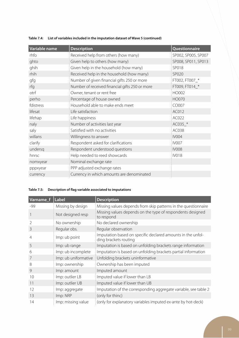
99
Variable name Description Questionnaire
rhfo Received help from others (how many) SP002, SP005, SP007
ghto Given help to others (how many) SP008, SP011, SP013
ghih Given help in the household (how many) SP018
rhih Received help in the household (how many) SP020
gfg Number of given financial gifts 250 or more FT002, FT007_*
rfg Number of received financial gifts 250 or more FT009, FT014_*
otrf Owner, tenant or rent free HO002
perho Percentage of house owned HO070
fdistress Household able to make ends meet CO007
lifesat Life satisfaction AC012
lifehap Life happiness AC022
naly Number of activities last year AC035_*
saly Satisfied with no activities AC038
willans Willingness to answer IV004
clarify Respondent asked for clarifications IV007
undersq Respondent understood questions IV008
hnrsc Help needed to reed showcards IV018
nomxyear Nominal exchange rate
pppxyear PPP adjusted exchange rates
currency Currency in which amounts are denominated
Table 7.5: Description of flag variable associated to imputations
Varname_f Label Description
-99 Missing by design Missing values depends from skip patterns in the questionnaire
1 Not designed resp Missing values depends on the type of respondents designed to respond
2 No ownership No declared ownership
3 Regular obs. Regular observation
4 Imp: ub point Imputation based on specific declared amounts in the unfol-ding brackets routing
5 Imp: ub range Imputation is based on unfolding brackets range information
6 Imp: ub incomplete Imputation is based on unfolding brackets partial information
7 Imp: ub uniformative Unfolding brackets uninformative
8 Imp: ownership Ownership has been imputed
9 Imp: amount Imputed amount
10 Imp: outlier LB Imputed value if lower than LB
11 Imp: outlier UB Imputed value if lower than UB
12 Imp: aggregate Imputation of the corresponding aggregate variable, see table 2
13 Imp: NRP (only for thinc)
14 Imp: missing value (only for explanatory variables imputed ex-ante by hot-deck)
Table 7.4: List of variables included in the imputation dataset of Wave 5 (continued)

100
ReferencesArnold, B.C., Castillo, E. & Sarabia, J.M. (1999). Conditional specification of statistical models. New York: Springer.
Arnold, B.C., Castillo, E. & Sarabia, J.M. (2001). Conditionally specified distributions: An introduction. Sta-tistical Science. 16, pp. 249-274.
Browning, M., Crossley, T.F. & Weber, G. (2003). Asking consumption questions in general purpose sur-veys. The Economic Journal. 133, p. 540-567.
Christelis, D. (2011). Imputation of missing data in Waves 1 and 2 of SHARE. SHARE WP Series, 01-2011.
Dardononi, V., Modica, S. & Peracchi, F. (2011). Regression with imputed covariates: a generalized mis-sing-indicator approach. Journal of Econometrics. 162, pp. 362-368.
Dardononi, V., De Luca, G., Modica, S. & Peracchi, F. (2014). Model averaging estimation of genera-lized linear models with imputed covariates. Journal of Econometrics, in press. doi: 10.1016/j.jeco-nom.2014.06.002.
Gelman, A. & Rubin, D.B. (1992). Inference from iterative simulation using multiple sequences. Statisti-cal Science. 7, pp. 457-511.
Gelman, A., Carlin, J.B., Stern, H.S. & Rubin, D.B. (2004). Bayesian data analysis. Second Edition. Boca Raton, FL: Chapman and Hall.
Lee, K.J. & Carlin, J.B. (2010). Multiple imputation for missing data: fully conditional specification versus multivariate normal imputation. American Journal of Epidemiology. 171, pp. 624-632.
Meng, X. (1994). Multiple-imputation inferences with uncongenial sources of input. Statistical Science. 9(4), pp. 538-558.
Raghunathan, T.E., Lepkowski, J.M., Van Hoewyk, J. & Solenberger, P. (2001). A multivariate technique for multiply imputing missing values using a sequence of regression models. Survey Methodology. 27, pp. 85–95.
Rubin, D.B. (1996). Multiple imputations after 18+ years. Journal of the American Statistical Association. 91, pp. 473-489.
Van Buuren, S. (2007). Multiple imputation of discrete and continuous data by fully conditional specifi-cation. Statistical Methods in Medical Research. 16, pp. 219-242.
Van Buuren, S., Brands, J.P.L., Groothuis-Oudshoorn, C.G.M. & Rubin, D.B. (2006). Fully conditional specifi-cation in multivariate imputation. Journal of Statistical Computation and Simulation. 76, pp. 1049-1064.
Van Buuren, S., Boshuizen, H.C. & Knook, D.L. (1999). Multiple imputation of missing blood pressure co-variates in survival analysis. Statistics in Medicine. 18, pp. 681- 694.

101
8 Fieldwork monitoring and survey participation in fifth wave of SHARE Thorsten Kneip, Frederic Malter, Gregor Sand, Munich Center for the Economics of Aging (MEA) at the Max Planck Institute for Social Law and Social Policy (MPISOC)
8.1 Introduction: conceptual and technological background
The purpose of this chapter is twofold: 1) to describe our efforts in fieldwork monitoring during the fifth wave of SHARE and 2) to report final outcomes of data collection in terms of response and retenti-on rates and shed some light on possible attrition bias.
The key innovation of Wave 5 was the revamping of the conceptual and technological backbone of fieldwork monitoring: we constructed all indicators strictly in accordance with standards set by the American Association of Public Opinion Research (AAPOR, 2015) and moved away from the less well-established indicators used in the previous waves of SHARE. This decision had two simple reasons: first, we wanted to be able to tell the SHARE community at any point in time what the response and retenti-on rates would be if fieldwork would be terminated at that given moment. Second, instead of running two different procedures – one during fieldwork and one after fieldwork - we found it more economical and conceptually straightforward to streamline the entire process: the final monitoring report is tanta-mount to the final outcome report on survey participation. Hence, both topics are now covered in this chapter. We first report what and how we monitored the progress of fieldwork and subsequently show the final outcomes.
Why fieldwork monitoring?
In any survey enterprise, ensuring data quality is a key concern (Lyberg and Biemer, 2008; Koch et al., 2009). Data quality of a survey has many facets which are most comprehensively conceptualized in the Total Survey Error (TSE) paradigm (Groves and Lyberg, 2010).
As in previous waves of SHARE, fieldwork monitoring comprised a set of activities aimed at minimi-zing selected components of the TSE while data collection was still on-going and corrective action was still possible. It is one of the many activities over the life cycle of a survey that can have a real impact on total survey error (Koch et al., 2009). Details on TSE can be found elsewhere (e.g. Groves and Lyberg, 2010). We will focus here less on the conceptual details but more on how we put the concept into ac-tion in this large survey operation.
Any survey enterprise has limited resources. Consequently, every survey operation makes choice – explicitly or implicitly – on how those resources will be allocated to achieve the ultimate goal, which is the collection of high-quality data. International survey operations may not be able to pay the same attention to each possible error source specified by TSE but may be forced to prioritize, be it for political, methodological, financial and/or human resource reasons. Errors or biases in survey statistics resulting from the misrepresentation of the target population – such as coverage error, sampling error or non-response error – make up the first of the two classes of the TSE. In SHARE, like in many other longitudi-nal studies, we made minimizing unit nonresponse our primary concern due to its quite unfavorable

102
consequences for panel studies (Watson and Wooden, 2009). Unit non-response, be it from lack of lo-cating the respondent, lack of establishing contact or lacking willingness to cooperate (Lepkowski and Couper, 2002) is the main cause of attrition in panel samples. Like in previous SHARE waves, we focused fieldwork monitoring again on activities aimed at minimizing the following three causes of unit nonre-sponse: a) difficulty of contacting households, b) gaining respondent cooperation, and c) dealing with cases of initial refusal. These activities all contribute to minimizing representational aspects of the TSE.
A second set of monitoring activities can be geared at reducing the second class of TSE errors, na-mely measurement errors (or even bias). One obvious source results from failure to conduct standar-dized interviewing. In the fourth wave of SHARE, we focused on the undesired interviewer behavior of not reading question texts properly. The most effective way would be to single out those interviewers that do not reach a specified threshold and make them aware of their undesired behavior. We decided against that strategy due to SHARE’s complex principal-agent structure: the interviewers are employees of private businesses that have contracts with SHARE to conduct fieldwork. We felt it would be at least inappropriate – if not outright at odds with labor laws – to report the underperforming of individual interviewers in a de-anonymized way. In other words, we discarded our initial idea of reporting perfor-mance indicators on the interviewer level. Instead, we - the central coordination team of SHARE at the Munich Center for the Economics of Aging (MEA) at the Max Planck Institute for Social Law and Social Policy (MPISOC) – understood our role as informing the contracted businesses and scientific country teams on a number of relevant indicators of fieldwork progress and data quality on the country level only. To that end, we sent out reports in a fortnightly fashion. Every other week, we released a fieldwork monitoring report. The goal of sending these reports to the survey agencies was to stimulate correc-tive action, i.e. make agency managers relay these findings to interviewers. The hope was that making interviewers aware of their being monitored would guide their behavior towards more successful and proper interviewing.
This type of fieldwork monitoring is, of course, dependent on an advanced IT infrastructure. Details about this IT infrastructure can be found elsewhere (Malter, 2013). Most representational indicators (i.e. those on unit nonresponse) were set out as quality targets in the specifications of the model contract. Details on these -contractually binding - standards can be found in the respective sections below.
Classification of sample units
Following the AAPOR guidelines, data from the SHARE Sample Management System (SMS) was used to classify the longitudinal and baseline/refreshment gross samples of each country into exhaustive and mutually exclusive categories reflecting the survey outcomes for each sample type. While this had already been done in Wave 4 to document survey participation ex post, it was now already incorporated in the fieldwork monitoring process. Therefore, all contact information entered into the SMS was conti-nuously translated into a so-called “household state”.
Table 8.1 shows how contact events recorded in the SMS translated into a household state. The algo-rithm which created the household state divided the sample into three mutually exclusive categories: (i) ineligible households, (ii) eligible households, and (iii) households of unknown eligibility1.
1 For details on SHARE’s target population and eligibility criteria see Kneip 2013.

103
SMS contact protocol entry Household state
Ineligible NE
Deceased3
In hospital3
In old-age home4
In prisonMoved abroadLanguage barriersMoved, new address unknown3
Address non-existent, house vacant3
No eligible persons after CVHousehold screened as ineligible5
Eligible E
Completed interview (incl. end-of-life interview) CI
Partial interview PI
Interrupted interview II
Refusal1 R
Too busy, no timeToo old, bad health conditionsNo interest, against surveysOther reasons
Other non-interview O
Contact, no appointmentContact, appointment for another contactContact, appointment for interviewDeceased3
In hospital3
In old-age home4
Moved, new address knownMoved, new address unknown3
Address non-existent, house vacant3
Household screened as eligible
Noncontact2 NC
Unknown eligibility UE
Screening refusal UER
Other screening non-cooperation UEO
Screening non-contact UENC
No contact attempted UENCA
Table 8.1: Detailed list of SMS entries and fieldwork outcomes at the HH level
Notes:1 For each category, interviewers could distinguish between a “soft” and a “hard” refusal, the latter one calling upon intervention from the agency. Neither of the refusal codes set by the interviewer closed a case.2 Noncontact for the eligible part of the sample does not apply to the baseline/refreshment sample in the Czech Republic.3 This led to ineligibility only in the baseline/refreshment sample, but not in the longitudinal sample.4 Whether this led to ineligibility in the baseline/refreshment sample depended on a country’s sampling frame. In the longitudinal sample, institutionalized cases were always considered eligible.5 Subcategories are: age ineligible household, problems with phone/address non-existent, language barriers.

104
This was done in a hierarchical way: once the eligibility status was determined, a new contact code could not revert the eligibility status into “unknown” anymore. Further, if a household was classified as ineligible, this was a “final state” which would permanently close a case, i.e. no more actions could be done by interviewers. The same applied to sorting households into sub-categories of the household state. A new contact only resulted in a change of the household state if it involved new information that would conceptually trump the previous information. For example, a household formerly classified as “noncontact” (NC) switched to “refusal” (R) after the interviewer had established contact but the respon-dent refused to participate. On the other hand, if an interviewer did not reach anybody (“noncontact”) in an attempt to convert a previous refusal (reflected in the household state “R” for refusal), the household state did not change but would stay at “R”. The fact that nobody opened the door to the interviewer did not make this particular household any more or less cooperative than before. The hierarchical order of the nexus “contact code–household state” is shown in Table 8.1 on the previous page.
Figure 8.1 shows the size of the longitudinal part of the sample in each country and how it was com-posed regarding household eligibility status. At the household level, the size of the longitudinal gross sample was defined by the number of households with at least one age-eligible respondent ever inter-viewed in any previous SHARE wave. This is because SHARE aims at recovering panel households that did not participate in a certain wave. For the purpose of fieldwork monitoring, the gross sample was determined by the number of households pre-loaded into the SMS, which lead to dropping households that could not be attempted again for legal reasons. Not surprisingly, the longitudinal gross samples contained almost exclusively eligible cases (97 percent).
Fiure 8.1: Panel samples by classification of sample units

105
Households in the longitudinal sample could only turn ineligible due to incarceration during the whole fieldwork period or moving abroad of all eligible household members or due to language bar-riers. On average, this applied to 0.6 percent of households in the longitudinal samples. Death did not lead to ineligibility. Instead, a proxy respondent was supposed to respond to an end-of-life interview about the deceased person. Households without any contact attempts were considered to be of un-known eligibility. Thus, a relatively large share of households with unknown eligibility can be interpreted as an indicator for poor fieldwork. However, it has to be noted that the figures below are solely based on information available through the SMS. If interviewers failed to enter contact attempts into the system, this could have led to a misclassification of household eligibility. On average, 2.2 percent of longitudinal households appear to have not been attempted for contact.
Figure 8.2 shows the size of the refreshment part of the sample or, respectively, the size of the baseline sample in Luxembourg (LU) and the Spanish region of Girona (Eg), all of which participated in SHARE for the first time in Wave 5. Averaging across countries, 84 percent of the gross samples were eligible, 11 percent were ineligible, and 5 percent were of unknown eligibility. In addition to the reasons leading to ineligibility in the longitudinal sample, baseline households were also considered ineligible in cases of death, in-patient treatment during the entire field time, moves with unknown or invalid ad-dresses, and if the cover screen interview yielded no eligible persons in the household. In the Czech Re-public, where the sample had to be screened for age eligibility first, (age-) ineligibility could also be an outcome of a screening contact. Thus, more general, in the baseline/refreshment sample the fraction of ineligible households reflected the availability and quality of sample frame information on which sampling was based. Accordingly, the fraction of ineligibles was highest in the Czech Republic, where the sample was based on the whole population and the sample frame did not contain any information on the household’s age composition. Any form of screening non-response (non-contact, refusal, other non-response) led to classifying a household as having “unknown eligibility”. Again, this fraction was rather pronounced in the Czech Republic, again mostly due to its sample frame. The highest fraction of non-attempted cases was observed in Israel but the rate was also non-negligible in Slovenia and in the French-speaking part of Belgium. In these countries, the share of non-attempted cases was also higher than in the longitudinal sample.
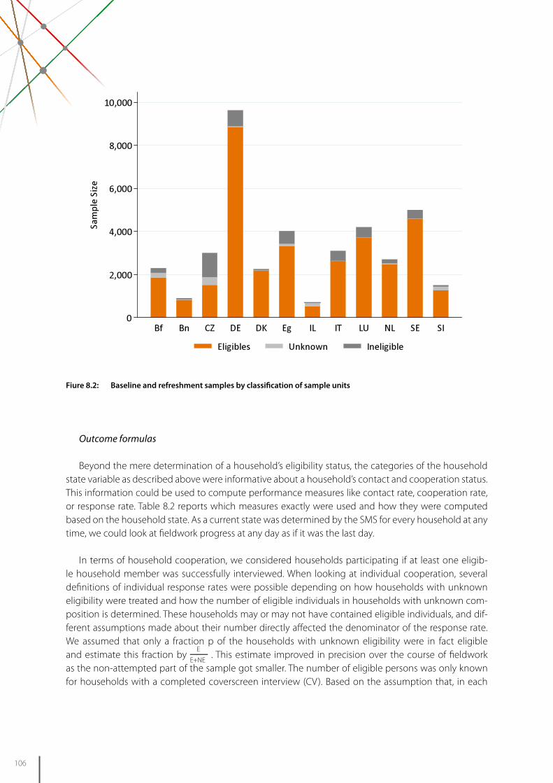
106
Fiure 8.2: Baseline and refreshment samples by classification of sample units
Outcome formulas
Beyond the mere determination of a household’s eligibility status, the categories of the household state variable as described above were informative about a household’s contact and cooperation status. This information could be used to compute performance measures like contact rate, cooperation rate, or response rate. Table 8.2 reports which measures exactly were used and how they were computed based on the household state. As a current state was determined by the SMS for every household at any time, we could look at fieldwork progress at any day as if it was the last day.
In terms of household cooperation, we considered households participating if at least one eligib-le household member was successfully interviewed. When looking at individual cooperation, several definitions of individual response rates were possible depending on how households with unknown eligibility were treated and how the number of eligible individuals in households with unknown com-position is determined. These households may or may not have contained eligible individuals, and dif-ferent assumptions made about their number directly affected the denominator of the response rate. We assumed that only a fraction p of the households with unknown eligibility were in fact eligible and estimate this fraction by . This estimate improved in precision over the course of fieldwork as the non-attempted part of the sample got smaller. The number of eligible persons was only known for households with a completed coverscreen interview (CV). Based on the assumption that, in each

107
country, the average number of eligible persons in households without CV did not systematically differ from that in households with CV, we took the latter as an estimate in the case of a baseline or refresh-ment sample. For households in the longitudinal sample without CV we could use preload information on household composition to assess the number of eligible respondents. Here the assumption was that this number did not change since the last interview, e.g. due to the moving-in of a new partner. If we estimated the average number of eligible respondents in a specific sample at , the total number of eligible respondents, and thus the denominator of the individual response rate, was (E+pUE).
Table 8.2: Outcome rate formulas
Estimated proportion of eligible households
Percentage of households attempted
Household contact rate (AAPOR CON2)
Household cooperation rate (cf. AAPOR COOP2)1
Household response rate (AAPOR RR4)
Household refusal rate (AAPOR REF2)
Household other non-interview rate (AAPOR ONI2)
Individual response rate2
Individual response rate in subsample i3
Notes:1 p(UE
R+UE
O) is not part of the denominator in AAPOR COOP2. The calculation method was adapted for
equation RR=CON×COOP to hold.2 is the average number of eligible persons per household. For baseline/refreshment sample is estimated based on households with completed coverscreen. For the longitudinal sample, information on household composition is available for all households from the previous wave. CI
r and PI
r refer to the number of com
pleted and partially completed interviews, respectively.3 is the average number of eligible persons from subsample i per household, where i = {A,B,C,D}.

108
In general, longitudinal samples can, at the individual level, be divided into four subsamples accor-ding to SHARE’s eligibility rules: subsample A includes all respondents who participated in the previous wave of the SHARE survey. Subsample B includes those respondents who ever participated in SHARE, but not in the previous wave, and live in a household where at least one household member participated in the previous wave. Subsample C includes respondents who ever participated, but not in the previous wave, and do not live in a household where at least one household member participated in the previous wave. Subsample D includes missing and new partners who have not participated in SHARE so far.
Response rates were reported separately for these subsamples during fieldwork. Note that individu-al-level retention in the narrow sense was then given by the proportion of respondents in subsample A participating in the fifth wave. Additionally, response in subsamples B and C depended on how well SHARE managed to bring respondents back who had already dropped out of the study for at least one wave. Finally, response in subsample D was relating to eligible persons in longitudinal households never interviewed before (i.e. either new sample members or eligible sample members who finally participa-ted after refusals in previous waves).
8.2 Fieldwork periods and survey agencies
For at least three reasons, the synchronized execution of fieldwork in all participating countries is a crucial requirement for an ex-ante harmonized survey like SHARE. First, from a scientific point of view, synchronicity of interview dates allows cross-country comparisons of effects of seminal events, such as external shocks (e.g. a financial crisis like the one in 2008/2009). Second, limited resources at central coordination make simultaneous monitoring of fieldwork necessary. Likewise, post-data collection pro-cessing of data, which ultimately yields data releases to the scientific community, relies on availability of all interview data at the same point in time. Data are never processed for countries individually, but always enter all-country processing procedures at the same point in time. In other words, one country being late has negative externalities for everybody else.
Figure 8.3: Fieldwork periods in SHARE Wave

109
As opposed to Wave 4, fieldwork in Wave 5 was conducted largely synchronous, see Figure 8.3 on the previous page. The beginning of fieldwork is indicated by receiving the Sample Distributor (SD) soft-ware that contains the preloaded samples, carrying out the national interviewer trainings, conducting the first interview, and providing the first data upload. In all countries except Luxembourg, the start of fieldwork was somewhere between mid-January and mid-March of 2013. Luxembourg started field-work in July. The end of fieldwork was marked by the
The organizations in Table 8.3 below conducted the fieldwork in each wave. There has been high stability of contracted survey agencies over time in most countries
Wave 1 Wave 2 Wave 3 Wave 4 Wave 5AT IMAS IMAS IFES IFES IFES
BE-FR PSBH,Liège Univ.
PSBH,Liège Univ.
PSBH,Liège Univ.
PSBH,Liège Univ.
CELLO - Antwerp Univ.
BE-NL PSBHAntwerp Univ.
PSBHAntwerp Univ.
CELLO - Antwerp Univ.
CELLO - Antwerp Univ.
CELLO - Antwerp Univ.
CH MIS Trend LINK LINK LINK LINK
CZ - SC&C SC&C SC&C SC&C
DE infas GmbH infas GmbH infas GmbH infas GmbH TNS Infratest
DK SFI-Survey SFI-Survey SFI-Survey SFI-Survey SFI-Survey
EE - - - Statistics Estonia GfK
ES TNS Demoscopia TNS Demoscopia TNS Demoscopia TNS Demoscopia TNS Demoscopia
ES-gi - - - - TNS Demoscopia
FR INSEE INSEE INSEE INSEE (panel)/ GFK-ISL (refresh.) GFK-ISL
IL - Cohen Institute,Tel Aviv Univ.
Cohen Institute,Tel Aviv Univ. - Cohen Institute,
Tel Aviv Univ.IT DOXA S.p.A. DOXA S.p.A. DOXA S.p.A. DOXA S.p.A. IPSOS
LU - - - - CEPS
NL TNS NIPO TNS NIPO TNS NIPO TNS NIPO TNS NIPO
SE Intervjubolaget IMRI
Intervjubolaget IMRI
Intervjubolaget IMRI
Intervjubolaget IMRI
Intervjubolaget IMRI
SI - - - CJMMK IPSOS
Table 8.3: Survey agencies from Wave 1 to 5 of countries participating in Wave 5
8.3 Reported indicators
This chapter includes all final rates and figures of Wave 5 based on the last data export on 2 Decem-ber 2013. A negligible number of interviews (N=10) had to be excluded that came in after our deadline of November 30, 2013. All numbers and figures reported during fieldwork were based on information

110
0.98 0.97 0.98 0.99
1.00 0.99 1.00 0.99
0.91 1.00 0.95 0.99
0.99 0.99 0.94
0.00.20.40.60.81.0
0.00.20.40.60.81.0
0.00.20.40.60.81.0
0.00.20.40.60.81.0
5 10 15 20 25 30 35 40 45
5 10 15 20 25 30 35 40 45 5 10 15 20 25 30 35 40 45 5 10 15 20 25 30 35 40 45
Austria Belgium (FR) Belgium (NL) Czech Republic
Denmark Estonia France Germany
Israel Italy Netherlands Slovenia
Spain Sweden Switzerland
% h
h att
empt
ed in
long
itudi
nal s
ampl
e
date of data extraction (calendar week)Graphs by country
Figure 8.4: Fraction of panel households with contact attempts by country
from the SHARE sample management system (SMS). This also applied to the trend charts depicted in this section. They reflect a “final monitoring report” after fieldwork was terminated. However, for the final numbers reported here, SMS data were cross-checked against data gathered during the CAPI interview. This cross-validation yielded only minimal deviations from SMS data. All findings are reported here for panel samples and refreshment or baseline samples separately. All indicators were graphed over calen-dar weeks to visualize each country’s progress of fieldwork over time. Final rates and interview numbers are then provided on in a final summary graph without trajectories. It must be kept in mind that the gross sample sizes differed drastically between countries which has direct effects for the progress of fieldwork. For example, it was much easier for Germany (N
panel household gross sample = 1035) to complete its
panel sample quickly than for France (Npanel household gross sample
= 5139). The last part of this chapter gives an outline of interviewer-based monitoring that was conducted at times to highlight specific fieldwork issues.
8.3.1 Panel samples
8.3.1.1 Contacting households
Figure 8.4 shows the fraction of households in the longitudinal gross sample where a contact was attempted, i.e. all households where either an interviewer reported a contact attempt but was unable to actually contact anybody or where a contact was successful (this includes, by definition, households with one or more conducted interviews).

111
In Wave 5, all countries except Israel, the Netherlands, and Switzerland managed to attempt nearly the entire panel samples. It has to be kept in mind that this does not necessarily reflect the intensity with which households were attempted for contact, for instance if a household ended up without an interview and was only attempted for a contact a single time It can be seen that most countries had a steep increase that levelled out over time, i.e. interviewers were quick at attempting the majority of all households for contact. France, Germany, and Switzerland deployed all their interviewer personnel from the very beginning. Countries such as Austria, Estonia, and Israel have a rather linear trend, possibly due to a different contact strategy. Figure 8.5 below shows country break-downs of household contact rates. This contains contact attempts which resulted in an actual contact, i.e. were a household member was reached. By definition, this may also include households with at least one complete interview.
0.96 0.95 0.96 0.98
0.99 0.97 0.99 0.99
0.89 0.99 0.93 0.98
0.97 0.98 0.94
0.00.20.40.60.81.0
0.00.20.40.60.81.0
0.00.20.40.60.81.0
0.00.20.40.60.81.0
5 10 15 20 25 30 35 40 45
5 10 15 20 25 30 35 40 45 5 10 15 20 25 30 35 40 45 5 10 15 20 25 30 35 40 45
Austria Belgium (FR) Belgium (NL) Czech Republic
Denmark Estonia France Germany
Israel Italy Netherlands Slovenia
Spain Sweden Switzerland
hh c
onta
ct ra
te, l
ongi
tudi
nal s
ampl
e
date of data extraction (calendar week)Graphs by country
Figure 8.5: Contact rate of panel households by country
With contact attempt rates being the logical ceiling to contact rates, Israel, the Netherlands, and Switzerland had the “lowest” contact rates. The trajectories of contact rates were similar to the rates on attempted households reported above.

112
0.78 0.73 0.76 0.74
0.750.89
0.640.80
0.880.71 0.67 0.78
0.78 0.680.87
0.00.20.40.60.81.0
0.00.20.40.60.81.0
0.00.20.40.60.81.0
0.00.20.40.60.81.0
5 10 15 20 25 30 35 40 45
5 10 15 20 25 30 35 40 45 5 10 15 20 25 30 35 40 45 5 10 15 20 25 30 35 40 45
Austria Belgium (FR) Belgium (NL) Czech Republic
Denmark Estonia France Germany
Israel Italy Netherlands Slovenia
Spain Sweden Switzerland
hh c
oope
ratio
n ra
te, l
ongi
tudi
nal s
ampl
e
date of data extraction (calendar week)Graphs by country
Figure 8.6: Cooperation rate of panel households by country
8.3.1.2 Household cooperation and response rate
Figure 8.6 below shows the cooperation rate of panel samples by country, i.e. the rate of all con-tacted households that had at least one completed interview. Despite low contact rates, Israel and Switzerland belong to the countries with the highest cooperation rates (88 percent and 87 percent respectively), outperformed only by Estonia (89 percent). The exact mirror image was France: one of the countries with the largest gross sample, it ended up with the lowest cooperation rate (64 percent) despite a very high contact rate (99 percent see Figure 8.5). This points to different mechanisms playing out when contacting households vs. gaining their cooperation. Austria, Estonia, and Israel remained at a cooperation rate of about 80 percent from the get-go, meaning that most household contacts resul-ted in at least one interview per household. In all other countries, cooperation rates kept increasing at different slopes until hitting a plateau, largely below 80 percent.

113
Figure 8.7 shows panel household retention rates, i.e. the number of panel households with at least one complete interview divided by the total number of (estimated) eligible panel households.
0.75 0.69 0.73 0.73
0.740.86
0.640.79
0.78 0.70 0.630.77
0.76 0.670.82
0.00.20.40.60.81.0
0.00.20.40.60.81.0
0.00.20.40.60.81.0
0.00.20.40.60.81.0
5 10 15 20 25 30 35 40 45
5 10 15 20 25 30 35 40 45 5 10 15 20 25 30 35 40 45 5 10 15 20 25 30 35 40 45
Austria Belgium (FR) Belgium (NL) Czech Republic
Denmark Estonia France Germany
Israel Italy Netherlands Slovenia
Spain Sweden Switzerland
hh re
spon
se ra
te, l
ongi
tudi
nal s
ampl
e
date of data extraction (calendar week)Graphs by country
Figure 8.7: Retention rate of panel households by country
It can be seen that again most countries had a steadily increasing trajectory that leveled out over time. Slovenia finished fieldwork in week 29, which is why the trajectory came to a rather abrupt stop. France, the Netherlands, and Sweden had the lowest household retention rates (keeping in mind that cooperation and contact rates represented the logical ceiling to the final retention rate). Estonia and Switzerland were the only countries which surpassed the 80 percent mark.
8.3.1.3 Individual participation
Figure 8.8 on the next page shows the individual retention rate of subsamples A and B. As pointed out before, subsample A included all respondents who participated in Wave 4; subsample B includes all respondents who participated in any previous SHARE wave, but not in Wave 4, and live in a household where at least one household member participated in Wave 4. SHARE stipulates at least 80 percent of respondents in these two subsamples combined be brought back in the current wave. Survey agencies were incentivized for rates exceeding 80 percent.

114
0.80 0.73 0.79 0.71
0.86 0.860.70 0.81
0.81 0.81 0.80 0.74
0.86 0.77 0.81
0.00.20.40.60.81.0
0.00.20.40.60.81.0
0.00.20.40.60.81.0
0.00.20.40.60.81.0
5 10 15 20 25 30 35 40 45
5 10 15 20 25 30 35 40 45 5 10 15 20 25 30 35 40 45 5 10 15 20 25 30 35 40 45
Austria Belgium (FR) Belgium (NL) Czech Republic
Denmark Estonia France Germany
Israel Italy Netherlands Slovenia
Spain Sweden Switzerland
indi
vidu
al re
spon
se ra
te, s
ubsa
mpl
es A
+B c
ombi
ned
date of data extraction (calendar week)Graphs by country
Figure 8.8: Individual retention rates in subsamples A and B by country
Belgium (both parts), the Czech Republic, France, and Slovenia, did not reach the expected minimum retention rate of 80 percent in subsamples A and B. In the Czech Republic and Slovenia the individual-level retention rate was slightly lower than the household retention rate suggesting that a significant number of known eligible spouses or partners could not be convinced to cooperate. It was reached by Austria and the Netherlands (80 percent), and surpassed by Germany, Israel, Italy, and Switzerland (81 percent). The front runners were Denmark, Estonia, and Spain (86 percent).

115
Figure 8.9 below shows the individual recovery rate of subsample C, i.e. the percentage of panel respondents that did not participate in Wave 4 (and any combination of [non-] participation in previous waves) but that were recovered in Wave 5.
0.27 0.27 0.22
0.49
0.300.22
0.35 0.39
0.33
0.11
0.35 0.41
0.0
0.2
0.4
0.6
0.8
1.0
0.0
0.2
0.4
0.6
0.8
1.0
0.0
0.2
0.4
0.6
0.8
1.0
5 10 15 20 25 30 35 40 45 5 10 15 20 25 30 35 40 45 5 10 15 20 25 30 35 40 45 5 10 15 20 25 30 35 40 45
Austria Belgium (FR) Belgium (NL) Czech Republic
Denmark France Germany Israel
Italy Netherlands Spain Sweden
indi
vidu
al re
spon
se ra
te, s
ubsa
mpl
e C
date of data extraction (calendar week)Graphs by country
Figure 8.9: Individual retention (recovery) rates in subsample C by country
Denmark, the Netherlands, and Sweden had the greatest absolute number of respondents in sub-sample C in Wave 5, while the Czech Republic had the smallest ones. Considering this, Sweden showed the best performance in bringing back as many “lost” respondents as possible, especially at the end of fieldwork. It is also interesting to point our different strategies used by survey agencies: Austria waited to the end of fieldwork to recover “lost” respondents whereas the opposite is true for the Czech Republic where the recovery rate leveled off at the mid-point of the fieldwork period.

116
0
.1
.2
.3
.4
.5
.6
.7
.8
.9
1
Rate
AT Bf Bn CH CZ DE DK EE ES FR IL IT NL SE SI
Contact Cooperation Response
Figure 8.10: Contact, cooperation and retention rates for panel households
8.3.1.4 Final outcomes of SHARE Wave 5
Figure 8.10 shows the final household contact, cooperation, and retention rates of the panel samples at the end of fieldwork Wave 5. Figure 8.10 does not contain new information over and above what was already reported but provides a quick reference to compare countries on their final outcomes.
Figure 8.11 on the next page shows the final individual retention rates by subsample. Apart from the above-defined subsamples A, B, and C, subsample D includes all non-responding spouses or partners and new spouses or partners that have not participated in any previous SHARE wave so far. For countries that joined SHARE in Wave 4 (Estonia and Slovenia), the classification into subsamples B and C was not applicable yet.

117
Figure 8.11: Respondent-level retention and recovery
Figure 8.12: Absolute numbers of interviews in panel samples
Figure 8.12 shows the absolute number of panel interviews per country at the end of fieldwork of Wave 5. Detailed breakdowns can be found in the appendix of this chapter.

118
8.3.1.5 Extrapolations
In weeks 19 and 31 of 2013 we complemented the bi-weekly reports with projections of the expec-ted fieldwork progress. The idea was born out of simple curiosity: given the information we have about the field today, what can we predict about the future? We then decided to expand this idea and employ it as a communication devise. By pointing out the anticipated trajectories, we could alert slow-moving countries to pick up speed in order to not underperform at the set end of fieldwork on 30 November 2013. We used two different scenarios to forecast response and retention rates: a linear extrapolation and – more realistic – a logarithmic extrapolation of growth rates. Figure 8.13 shows these extrapolations for retention rates in subsamples A and B as of week 31, the initially planned end of fieldwork (marked by the vertical lines). The horizontal line at 80 percent marks the minimum retention rate as stated in the model contract. At this point in time, projections for some countries indicated that non-compliance to the 80 percent minimum retention rate was to be expected without ramping up their efforts.
When compared to the final actual response rates, (logarithmic) projections turned out to be fairly predicti-ve in most countries (c.f. figure 8.8). However, some countries fell short of the predicted outcome, namely Bel-gium (both parts) and the Czech Republic. On the other hand, there were countries that exhibited an accele-rated growth towards the end of fieldwork, surpassing the projected rate, namely Estonia, Spain, and Sweden.
0.00.20.40.60.81.0
0.00.20.40.60.81.0
0.00.20.40.60.81.0
0.00.20.40.60.81.0
5 9 13 17 21 25 29 33 37 41 45
5 9 13 17 21 25 29 33 37 41 45 5 9 13 17 21 25 29 33 37 41 45 5 9 13 17 21 25 29 33 37 41 45
Austria Belgium (FR) Belgium (NL) Czech Republic
Denmark Estonia France Germany
Israel Italy Netherlands Slovenia
Spain Sweden Switzerland
actual rate extrapolation (lin.) extrapolation (log)
indi
vidu
al r
espo
nser
ates
, sub
sam
ples
A+B
com
bine
d
date of data extraction (calendar week)
Graphs by country
Figure 8.13: Extrapolation of retention rates in subsamples A+B, week 31

119
Overall, we found the exercise of computing and communicating these rates a useful vehicle to manage fieldwork and give momentum especially to those countries lagging behind in terms of improving response beyond the initially planned end of fieldwork. 8.3.2 Refreshment samples
8.3.2.1 Contacting households
Figure 8.14 shows the fraction of households in the of households in the refreshment/baseline gross sample where a contact was attempted, i.e. all households where either an interviewer reported a con-tact attempt but was unable to actually contact anybody or where a contact was successful (this inclu-des, by definition, households with one or more conducted interviews).
0.900.98 0.98 1.00
1.00 0.97
0.77
1.00
1.00 0.980.89
1.00
0.0
0.2
0.4
0.6
0.8
1.0
0.0
0.2
0.4
0.6
0.8
1.0
0.0
0.2
0.4
0.6
0.8
1.0
5 10 15 20 25 30 35 40 45 5 10 15 20 25 30 35 40 45 5 10 15 20 25 30 35 40 45 5 10 15 20 25 30 35 40 45
Belgium (FR) Belgium (NL) Czech Republic Denmark
Germany Girona Israel Italy
Luxembourg Netherlands Slovenia Sweden
% h
h att
empt
ed in
bas
elin
e /
refr
eshm
ent s
ampl
e
date of data extraction (calendar week)Graphs by country
Figure 8.14: Fraction of refreshment/baseline households with contact attempts by country
In Wave 5, Israel, Belgium (FR), and Slovenia did not exhaust their refreshment samples in terms of contact attempts. Slovenia discontinued fieldwork in week 29 after reaching a predetermined target number of interviews. Similar to the panel samples, most countries had a steep increase that leveled out over time. The observable drops in the Spanish region of Girona, the Czech Republic, and Denmark were due to the activation of new batches in the respective countries that temporarily altered the proportion

120
0.820.90 0.90
0.98
0.98 0.93
0.71
0.98
0.95 0.930.82
0.95
0.0
0.2
0.4
0.6
0.8
1.0
0.0
0.2
0.4
0.6
0.8
1.0
0.0
0.2
0.4
0.6
0.8
1.0
5 10 15 20 25 30 35 40 45 5 10 15 20 25 30 35 40 45 5 10 15 20 25 30 35 40 45 5 10 15 20 25 30 35 40 45
Belgium (FR) Belgium (NL) Czech Republic Denmark
Germany Girona Israel Italy
Luxembourg Netherlands Slovenia Sweden
hh c
onta
ct ra
te, b
asel
ine/
refr
eshm
ent s
ampl
e
date of data extraction (calendar week)Graphs by country
Figure 8.15: Contact rate of refreshment/baseline households by country
of attempted and un-attempted households (for details on the strategy of replicates or “batches”, see chapter 3). Luxembourg joined fieldwork with their baseline sample in the middle of Wave 5 and put great effort into catching up and finishing fieldwork on time.
Figure 8.15 shows household contact rates broken down for countries. This contains contact att-empts which resulted in an actual contact. By definition, this may also include households with at least one completed interview.
Not surprisingly, a similar picture emerged as above. As a result of not having attempted all households for contact, Israel, Belgium (FR), and Slovenia had the lowest contact rates.

121
8.3.2.2 Household cooperation and response rate
Figure 8.16 shows the cooperation rate of refreshment/baseline samples by country, i.e. the rate of all contacted households that have at least one completed interview.
Cooperation rates are based only on sample units with a previous contact. The interpretation of cooperation rates becomes more meaningful as contact rates increase. This is accompanied by a stabi-lization of cooperation rates over the fieldwork period. For instance, the Czech Republic had contacted a fairly small number of households after starting fieldwork in week 17. Many of these households co-operated, which explains the near-vertical slope. However, afterwards the number of contacted house-holds grew faster than the number of households with at least one completed interview so cooperation rates leveled out at a lower rate. Despite of the lowest contact attempt and contact rates, Israel has the highest rate of household cooperation (73 percent), followed by the Spanish region of Girona (65 percent). Belgium (FR, 38 percent), Germany (35 percent), and Luxembourg (34 percent) had the lowest cooperation rates because of high rates of refusal (see Appendix of this chapter).
0.380.47
0.61 0.60
0.35
0.650.73
0.44
0.34
0.52 0.500.41
0.0
0.2
0.4
0.6
0.8
1.0
0.0
0.2
0.4
0.6
0.8
1.0
0.0
0.2
0.4
0.6
0.8
1.0
5 10 15 20 25 30 35 40 45 5 10 15 20 25 30 35 40 45 5 10 15 20 25 30 35 40 45 5 10 15 20 25 30 35 40 45
Belgium (FR) Belgium (NL) Czech Republic Denmark
Germany Girona Israel Italy
Luxembourg Netherlands Slovenia Sweden
hh c
oope
ratio
n ra
te, b
asel
ine/
refr
eshm
ent s
ampl
e
date of data extraction (calendar week)Graphs by country
Figure 8.16: Cooperation rate of refreshment/baseline household by country

122
0.310.42
0.55 0.59
0.34
0.600.52
0.43
0.33
0.490.41 0.39
0.0
0.2
0.4
0.6
0.8
1.0
0.0
0.2
0.4
0.6
0.8
1.0
0.0
0.2
0.4
0.6
0.8
1.0
5 10 15 20 25 30 35 40 45 5 10 15 20 25 30 35 40 45 5 10 15 20 25 30 35 40 45 5 10 15 20 25 30 35 40 45
Belgium (FR) Belgium (NL) Czech Republic Denmark
Germany Girona Israel Italy
Luxembourg Netherlands Slovenia Sweden
hh re
spon
se ra
te, b
asel
ine/
refr
eshm
ent s
ampl
e
date of data extraction (calendar week)Graphs by country
Figure 8.17: Response rate of refreshment/baseline households by country
Figure 8.17 shows the household response rate, i.e. the number of refreshment/baseline households with at least one complete interview divided by the total number of (estimated) eligible refreshment/baseline households.
Many countries had steadily increasing trajectories. The Spanish region of Girona, the Czech Repub-lic, Denmark, and Israel achieved successful cooperation in more than 50 percent of their refreshment sample. The Spanish region of Girona was the front runner with 60 percent of household response. Similar to the panel sample, the good performance of Israel in household cooperation is dampened by a comparably low household response rate due low contact rates. At a lower level, this is also the case in Belgium (FR) and Slovenia.

123
8.3.2.3 Individual participation
Figure 8.18 shows the individual response rate of refreshment/baseline samples in Wave 5.
The trajectories of the individual response rates in all countries were fairly similar to the household response rates, again with the Spanish region of Girona having the highest individual response rate (57 percent). Individual participation was consistently lower than household response because spouses or partners could not be convinced to cooperate. Belgium (FR) and Luxemburg and failed to reach the demanded minimum individual response rate of 30 percent.
8.3.2.4 Final rates and numbers
Figure 8.19 on the next page shows the final household contact, cooperation, and response rates at the end of fieldwork Wave 5.
Figure 8.18: Individual response rate of refreshment/baseline respondents by country
0.260.37
0.51 0.51
0.30
0.570.44 0.41
0.250.40
0.32 0.33
0.0
0.2
0.4
0.6
0.8
1.0
0.0
0.2
0.4
0.6
0.8
1.0
0.0
0.2
0.4
0.6
0.8
1.0
5 10 15 20 25 30 35 40 45 5 10 15 20 25 30 35 40 45 5 10 15 20 25 30 35 40 45 5 10 15 20 25 30 35 40 45
Belgium (FR) Belgium (NL) Czech Republic Denmark
Germany Girona Israel Italy
Luxembourg Netherlands Slovenia Sweden
indi
vidu
al re
spon
se ra
te, b
asel
ine/
refr
eshm
ent s
ampl
e
date of data extraction (calendar week)Graphs by country

124
Figure 8.19: Contact, cooperation and response rates for baseline/refreshment samples
Figure 8.20: Household and respondent-level survey participation in baseline/refreshment samples
Figure 8.20 shows the final household and respondent-level response rates.

125
8.3.2.5 Total number of interviews
Figure 8.21 shows the absolute number of interviews per country in the refreshment/baseline sam-ples at the end of fieldwork Wave 5.
Figure 8.21: Absolute number of interviews in baseline/refreshment samples
8.3.2.6 Extrapolations
Together with the projected retention rates in panel subsamples A and B we also reported projec-tions for baseline and refreshment samples in weeks 19 and 31 of 2013. Figure 8.22 shows the report-ed figures of week 31. Luxembourg is not reported because it had just started their fieldwork. Again, logarithmic extrapolations turned out to be fairly predictive when compared to fieldwork outcomes (s. Figure 8.17). This even held for countries that used sample batches, although actual curve progressions looked very differently due to the drops after opening new batches. And again, some countries slightly deviated from the general pattern: curves leveled off earlier than expected in the Dutch-speaking part of Belgium, Italy, and, in Slovenia due to abrupt termination of fieldwork. In Sweden, on the other hand, the acceleration in growth towards at the end of fieldwork could also be observed in the refreshment sample. Overall, the reporting of these numbers did not have much impact in terms of lifting response rates above the target of 50 percent when projections indicated a shortfall.

126
0.0
0.2
0.4
0.6
0.8
1.0
0.0
0.2
0.4
0.6
0.8
1.0
0.0
0.2
0.4
0.6
0.8
1.0
5 9 13 17 21 25 29 33 37 41 45
5 9 13 17 21 25 29 33 37 41 45 5 9 13 17 21 25 29 33 37 41 45 5 9 13 17 21 25 29 33 37 41 45
Belgium (FR) Belgium (NL) Czech Republic Denmark
Germany Girona Israel Italy
Netherlands Slovenia Sweden
actual rate extrapolation (lin.) extrapolation (log)
hh r
espo
nse
rate
, bas
elin
e /
refr
eshm
ent s
ampl
e
date of data extraction (calendar week)
Graphs by country
Figure 8.22: Extrapolation of household response rate in baseline/refreshment samples, week 31

127
8.4 Monitoring of interviewer activity and interventions by SHARE Central
Apart from reporting the AAPOR-based fieldwork indicators in our biweekly monitoring reports, two supplementary reports highlighted fieldwork issues at specific times of Wave 5. The first supplement was sent out at the early stage of fieldwork and provided an overview of the number of interviewers that had been trained and active during the first four data upload periods (or roughly eight weeks of fieldwork). This was done to get an idea of the rate of active interviewers as share of the total intervie-wer workforce. The second supplement was sent out in the middle of fieldwork after detecting the following:
• inconsistencies in reported numbers of trained interviewers, • low rates of interviewer activity across many countries, • fluctuations of activity among individual interviewers and • exceptionally high numbers of interviews by some interviewers.
The following paragraphs will briefly outline fieldwork issues and related feedback we received from survey agencies.
8.4.1 Inconsistencies in reported numbers of trained interviewers vs. “visible” interviewers
Survey agencies reported the number of trained interviewers, which was used as denominator to compute the percentage of active interviewers (see next section). In the middle of fieldwork, we com-pared the number of trained interviewers to the number of interviewers registered through the Sample Distributor (SD), i.e. those that actually entered the SHARE IT system and thus became “visible” to us. The number of interviewers visible in the SD was taken as the maximum number of interviewers that could be active in the field at any given point in time. In several countries we found a negative difference bet-ween the numbers of trained and visible interviewers (e.g. 90 interviewers reported to be trained, but only 80 visible in the SD). This means that either fewer interviewers were trained than reported or that some of the trained interviewers never worked for SHARE in Wave 5. In order to correct our documented numbers, we asked all agencies with a negative difference (i.e. smaller than -2) to let us know what hap-pened with the seemingly over-reported number of interviewers. The result was that about 40 percent of the “over-reported” interviewers were actually never trained and the remaining 60 percent dropped out after being trained. The most prominent reasons for dropping out were health issues, increasing workload in the main job, the decision to not participate in the study, or a lack of skills to work for SHARE (for a more detailed list of reasons see section 8.4.2.).
8.4.2 Rate of active interviewers over time
The rate of active interviewers is the ratio of interviewers with any activity in the Sample Manage-ment System (SMS) divided by the number of trained interviewers, as reported by agencies (see above). An interviewer was considered “active” as soon as any kind of information (e.g. contact attempt, appoint-ment, remark, or completed interview) was registered by the SMS.

128
Figure 8.23 shows the rate of active interviewers over time up to week 31 (end of July 2013), the date we sent out the second supplement to our monitoring reports (selected countries only).
020406080
100
020406080
100
020406080
100
020406080
100
5 7 9 11 13 15 17 19 21 23 25 27 29 31 5 7 9 11 13 15 17 19 21 23 25 27 29 31 5 7 9 11 13 15 17 19 21 23 25 27 29 31 5 7 9 11 13 15 17 19 21 23 25 27 29 31
Austria Belgium (FR) Belgium (NL) Czech Republic
Denmark Estonia France Germany
Girona Israel Italy Netherlands
Slovenia Spain Sweden Switzerland
% a
ctiv
e in
terv
iew
ers
date of data extraction (calendar week)Graphs by country
Figure 8.23: Rate of active interviews over time during the first half of fieldwork
Figure 8.23 highlights a number of important features of fieldwork in the participating countries. Each country’s trajectory can be partitioned into the three phases of fieldwork: beginning, middle and end. Note that the actual calendar time of those phases varied by country. In an ideal world, a high rate of trained interviewers would be deployed quickly (within 4-8 weeks after the first trainings con-sidering that training the entire pool usually takes about 4 weeks), signaling a prioritization of SHARE fieldwork over other potential projects of the contracted survey agency. After a “sudden onset”, main-taining a high rate of interviewers active in the field would indicate a strategy that aims at completing the majority of fieldwork before the summer break. This strategy was highly recommended by SHARE because many respondents will be harder to reach during summer vacations (which vary a lot between countries with respect to onset and duration). No performance-related statement can be made about the end of fieldwork: a sudden end can mean different things: forceful termination of fieldwork despite under-exhausted potential (e.g. households without contact), which is clearly undesirable. Or it could indicate that only very few of active interviewers are now deployed to deal with the remaining difficult cases. The same logic applies to a gradual end of fieldwork: it could mean that a higher activity during the middle of fieldwork was not achieved so hence the end would take longer or it may indicate that in-terviewers are wrapping up one by one, a perfectly fine strategy. Note the decline in interviewer activity

129
in almost all countries approaching week 31, the initially planned end of fieldwork. This decline is visible for countries that had achieved the required minimum retention rate of 80 percent in subsamples A+B by that time, but also for some countries that had not reached this rate yet (see Fig. 8.13).
We communicated our concerns with the hope of inducing corrective action on the side of the sur-vey agency by asking all survey agencies with low rates of active interviewers, i.e. those countries with a low plateau and inconsistent activity of individual interviewers in week 23 of 2013 to answer some ques-tions. We report here the most commonly mentioned responses for mismatches between number of trained and visible interviewers and low rates of active interviewers in Figure 8.23 (i.e. in week 23 of 2013):
• Interviewers didn’t want to work for SHARE after they received information on SHARE study due to its high requirements. • Low rate of active interviewers due to high number of sequential trainings (not all interviewers were
trained at the same time and therefore not all interviewers could be active at the same time).• New interviewers didn’t want to put on that much workload for SHARE for the given salary.• Some interviewers dropped out before or shortly after training (health, family, personal or
time issues). • Not all interviewers had been trained at that point.• Waiting for more experienced interviewers, which were not available for SHARE, yet. • Interviewers were considered not qualified enough to work for SHARE and were therefore excluded
from the survey.• Interviewers work on temporary basis and work for other surveys at the same time. • Interviewers were on holidays before the summer. • Some dropped out of SHARE altogether because of the length of the questionnaire. • Some interviewers were just “slow workers”.• Technical problems with SD: More interviewers in SD than participating in fieldwork.
8.4.3 Fluctuations of activity among individual interviewers
The statistic of “rate of active interviewers” (Figure 8.23 on the previous page) did not allow any con-clusion if it were the same interviewers that were active in a given period or different interviewers (i.e. the net change from period to period). In order to shed light on how active individual interviewers were, we computed a sum score across all data export dates in week 23. If an interviewer was active during all weeks between week 11 and week 23, he or she would get a sum score of seven (seven export periods times one). If an interviewer was active for less than seven export periods he or she got a lower score (for example any combination of two export periods yielded a score of two, see Figure 8.24 on the next page). Note that the time between weeks 11 and 23 should have corresponded to the main phase of fieldwork for most countries. At that period, we would have expected a very high activity by the majo-rity of interviewers.

130
Figure 8.24: Number of active weeks per interviewer
It can be seen, for example, that in Germany and Switzerland most interviewers have worked in all weeks between week 11 and week 23. A similar picture emerged for Belgium and Slovenia.
A very different picture emerged for most other countries: most interviewers have only been active for a part of the period between week 11 and week 23.
These were the main reported reasons for inconsistent activity rates of many interviewers in most countries:
• SHARE had different priority for different interviewers. Interviewers have different number of households to contact due to late start or vacation. • Interviewers were bound to certain regions and couldn’t be used elsewhere.• During certain times of the year (holidays, etc.) interview rates had to go down automatically. • Interviewers live in areas (e.g. islands) with very few respondents.
Overall, apart from health and seasonal factors, issues in recruitment and effectively deploying in-terviewers, as well as motivational issues on the part of interviewers appeared to be most relevant for explaining low levels of interviewer activity across many countries and fluctuations of activity among a large share of interviewers.

131
8.4.4 Number of interviews per interviewer
In Wave 5, SHARE stipulated that no interviewer conduct more than 50 interviews in total with the goal of avoiding “interviewer effects”, i.e. responses (or non-responses) that occur because of clustering too many respondents within the same interviewer(s). An example would be non-response to income questions clustered within particular interviewers: it was plausible to assume that an interviewer who felt uneasy about asking respondents for their income, SHARE would end up with high rates of miss-ing income data for the entire country if that interviewer would have conducted a large number of interviews. Interviewer training was one way to reduce this problem. Another way was our attempt at limiting the number of interviews per interviewer by recommending the training of a sufficient number of interviewers given the desired number of interviews.
In Wave 5, no country remained within the 50-interviews limit completely, but we observed large differences between countries (see Figure 8.25). While the majority of interviewers conducted less than 50 interviews, we detected some interviewers exceeding 100 interviews. For this reason, we wanted to know why the workload was so unevenly distributed across interviewers and if agencies saw a pos-sibility to restrict the number of interviews per interviewers. We received very homogenous feedback on the latter: even though some efforts were made to stay within the limit, the majority of all countries did not see a possibility to restrict the number of interviews. The unevenly distributed workload was explained by a variety of reasons: budgetary constraints topped the list. Strategy-wise it was argued that experienced and persuasive interviewers were assigned more households, while less experienced and new interviewers were assigned fewer households; apart from that, strong clustering of households within certain primary sampling units (PSU) played an important role because in many cases the sam-ples were not distributed evenly across the country or it was hard to find good interviewers in some re-gions. Other reasons were directly related to interviewer tenure, e.g., full-time interviewers can do more work than part-time interviewers; and some interviewers quit the job or were laid off during fieldwork.

132
010
2030
400
1020
3040
010
2030
400
1020
3040
0 100 200 300 0 100 200 300 0 100 200 300 0 100 200 300
at be_fr be_nl ch
cz de dk ec
ee es fr il
it nl se si
Freq
uenc
y
Number of interviews per interviewerData available at week 23
Figure 8.25: Number of interviews per interviewer in week 23

133
8.5 Beyond fieldwork monitoring: development of sample composition among the SHARE longitudinal samples
Thus far, we have treated longitudinal preload samples in the same way as baseline gross samples, showing the same contact, cooperation and response rates of Wave 5 for both types of samples. From the perspective of fieldwork monitoring, this was a reasonable procedure. From a data user´s perspec-tive however, the value of a longitudinal sample will be strongly determined by its long-term retention rate and the selectivity of attrition of panel members over waves. Figure 8.26 complements the previous findings by showing the development of all SHARE samples over time, hence combining retention and recovery. Figures below always refer to data publicly released for Waves 1-4; numbers of the fifth wave were based on a preliminary internal release version (also see Appendix).
0
1,000
2,000
3,000
4,000
5,000
6,000
7,000
AT BE CH CZ DE DK EE ES Eg FR GR HU IE IL IT LU NL PL PT SE SI
12345 12345 12345 12345 12345 12345 12345 12345 12345 12345 12345 12345 12345 12345 12345 12345 12345 12345 12345 12345 12345
Baseline sample Refreshment sample 1Refreshment sample 2 Refreshment sample 3
Figure 8.26: Overview of SHARE samples up to Wave 5
Analyses of panel data, like those collected in SHARE, make use of change over time. To conduct such analyses, respondents need to be observed at multiple points in time. With high attrition rates the number of cases in the panel decreases quickly, effectively reducing the power of longitudinal analyses. Moreover, attrition from the panel might affect the sample composition, as certain groups of respon-dents might be more likely to drop out of the panel than others. In the following, we shortly summarize our findings on differential attrition among major sub-groups of the SHARE longitudinal samples.
After five waves, various types of retention rates could be calculated. For example, retention rates may be calculated with regards to all units that have ever entered the panel, or all units participating in the previous wave, or all units not participating in the previous wave, or really any possible participation pattern over the Waves 1 to 4. To maximize comparability with Blom and Schröder (2011), we focus here

134
Figure 8.27: Household retention rates across countries participating in Wave 5 by sample 2
on retention rates from Wave 4 to Wave 5. Note that this does not include recovered cases, i.e. those who were brought back in Wave 5 after missing Wave 4. As Blom and Schröder (2011) have shown, attrition tends to be higher when panel members were approached for the first re-interview than at later waves. Therefore, we distinguished between the sample members for whom Wave 5 was the first re-interview, and the long-term sample members who participated since Wave 1 or Wave 2 (see Figures 8.27 and 8.28). Figure 8.27 shows the household retention rates for each country participating in Wave 5 by the different samples (absolute number of interviews can be found in Appendix 2). No bars are displayed when no baseline or refreshment sample was fielded in the respective year. As can be seen, the variation in household retention rates of Wave 5 across countries was considerable, ranging from 67 percent in Germany to 89 percent in Denmark for the older samples and from 58 percent in Italy to 87 percent in Denmark for the Wave 4 samples. This variation was caused by differences between countries in legal restrictions to approach respondents refusing in a previous wave, in fieldwork procedures and in general survey climate. The graph also confirms higher attrition at the first re-interview than at subse-quent waves (not across the board, however). This is indicated by the dark grey bars being the smallest in six out of the nine countries where the comparison was possible.
2 Note that figures 8.27, 8.28, 8.29 and 8.30 do not include recovered cases, i.e. those who were brought back in Wave 5 after missing Wave 4.

135
The individual retention rates (Figure 8.28) differ only slightly from the household retention rates. This is due to the large proportion of two-person households in which two interviews or more were completed (86 percent of two-person households across all countries).
Figure 8.28: Individual retention rates across countries participating in Wave 5 by sample
As described above, panel attrition not only harms the power of longitudinal analyses by decreasing sample size over time, but it can also affect the representativeness of the sample if specific sub-groups of panel members drop out more than others. Consequently, we compare individual retention rates at the transition from Wave 4 to Wave 5, between gender and age groups.

136
Figure 8.29: Individual retention rates by gender
With respect to gender, Figure 8.29 shows that, overall, retention seems slightly higher amongst women than men. This difference was significant only in the Czech Republic, Estonia, Spain and the Netherlands. In most SHARE countries, attrition is not strongly related to gender.
In a study investigating health and ageing, retention rates by age groups are of particular interest. Specifically, morbidity-related attrition is a potential concern amongst the ‘oldest old’. The individual retention rates by age groups, presented in Figure 8.30, somewhat validated this concern: in almost all countries the oldest quartile of respondents had a significantly lower propensity to stay in the panel. Furthermore, in some countries (e.g. CZ, IT) the youngest respondents are also more likely to drop out of the panel. These findings are contrary to what has been found for the transition to Wave 3 (Blom and Schröder, 2011).

137
Figure 8.30: Individual retention rates by age group
Overall, no consistent gender-related attrition bias was found across SHARE countries participating in Wave 5. There was, however, an indication that the oldest respondents are more likely to drop out. However, it must be kept in mind that numbers in Figure 8.30 were not adjusted for actual mortality (mostly due to a lack of sound mortality data). An adjustment for actual mortality would improve the retention rates among the oldest age group. Further research will be needed to disentangle the me-chanisms behind this differential retention, which we plan on doing. As mentioned above, since much is already known about dropped out respondents from their participation in previous waves, selectivity due to panel attrition can – and probably should – always be accounted for in statistical models. We provide data users with weighting procedures that may help in controlling for potential retention bias (see chapter 6 of this book).

138
8.6 Conclusions and outlook
For the fifth wave of SHARE, we put fieldwork monitoring on a new conceptual and technological foundation. We brought the reported indicators in line with standard definitions by AAPOR used around the globe to report fieldwork outcomes of scientific survey studies and established a work flow that would automatically yield final rates at the end of fieldwork. Hence, we eliminated the necessity to put effort into creating final outcome numbers as they were identical with the final monitoring status. The result was more efficiency. We will definitely continue this new procedure in Wave 6. For the first time, we created extrapolations of expected end of fieldwork for all countries and fed this info back to survey agencies. We found the exercise of computing and communicating these rates a useful vehicle to ma-nage fieldwork and give momentum especially to those countries lagging behind in terms of improving response beyond the initially planned end of fieldwork. Overall, fieldwork of participating countries was much more synchronous than in Wave 4.
We found very high contact rates (≥95 percent), but only moderate cooperation rates among panel household in most countries (between 70 and 80 percent). Two thirds of countries reached or surpassed the contractual minimum retention rate of 80 percent in subsamples A & B, and about one third of countries fell below this cut-off. When looking at the transition from Wave 4 to Wave 5, we found little evidence for attrition bias with respect to gender or age, apart from the oldest old being more likely to drop out. The majority of countries also had very high contact rates (≥95 percent) among baseline households, but three countries reached only about 80 percent or less. Cooperation among refresh-ment households was rather low (between 30 and 40 percent) in most countries, with exceptions in CZ, DK, and IL all of which made 60 percent or more of their contacted baseline households participate in the survey. Respondent-level response rates were low (<30 percent) only in Luxembourg, and moderate (between 30 and 40 percent) to high (50 percent and more) in all other countries.
SHARE has a very different business model for its field work than other aging surveys, notably the Health and Retirement Study (HRS) in the US, with a complex governance structure. SHARE subcontracts independent survey agencies which in turn hire independent interviewers. They were almost always self-employed (this reduces fringe benefits) and were usually paid by piece rather than by hour. These conditions were determined by national labor and social security laws and out of our control. When we discovered issues in interviewer activity, we sought input from survey agencies as to why activity patterns were so variable and partly so low. We did not have direct influence on the interviewers except during training. While we learned a lot about different interviewer management between countries, it is our impression that once training was over, interviewers were largely self-determined with little possibi-lity of survey agencies – and even less by us – to intervene. Since almost all survey agencies employed interviewers on a part-time, free-lance basis with payment per completed interview, interviewers were able to choose their own priorities when balancing other projects with their SHARE workload. Finally, most survey agencies reported difficulties in recruiting enough interviewers with sufficient skills and ex-perience to conduct SHARE. It seems that a different payment system and offering actual employment tenure (with possibilities of promotion) could help solve some of the problems but this would require a long-term funding scheme for SHARE which we do not have.

139
ReferencesAmerican Association of Public Opinion Research (2015). Standard definitions. Final dispositions of case codes and outcome rates for surveys. Retrieved from http://www.aapor.org/AAPORKentico/AAPOR_Main/media/publications/Standard-Definitions2015_8theditionwithchanges_April2015_logo.pdf.
Blom, A. & Schröder, M. (2011). Sample composition 4 years on: retention in SHARE Wave 3. In: Schröder, M. (Ed.). Retrospective Data Collection in the Survey of Health, Ageing and Retirement in Europe, pp. 55-61. SHARELIFE Methodology, Mannheim: MEA.
Groves, R. & Lyberg, L. (2010). Total survey error: past, present and future. Public Opinion Quarterly. 74(5), pp. 849-879.
Kneip, T. (2013). Survey participation in the fourth wave of SHARE. In: Malter, F. & Börsch-Supan, A. (Eds.). SHARE Wave 4: Innovations & Methodology, pp. 140-155. Munich: MEA.
Koch, A., Blom, A., Stoop, I. & Kappelhof, J. (2009). Data collection quality assurance in cross-national surveys: the example of the ESS. Methoden-Daten-Analysen.3, pp. 219-247.
Lepkowski, J. & Couper, M. (2002). Nonresponse in the second wave of longitudinal household surveys. In: Groves, R.M., Dillman, D.A., Eltinge, J.L. & Little, R.J.A. (Eds.). Survey Nonresponse, pp. 259-272. New York: John Wiley & Sons, Inc.
Lyberg, L. & Biemer, P. (2008). Quality assurance and quality control in surveys. In: de Leeuw, E., Hox, J. & Dillman, D. (Eds.). International Handbook of Survey Methodology, pp. 421-441). New York: Psychology Press.
Malter, F. (2013). Fieldwork monitoring in the Survey of Health, Ageing and Retirement in Europe (SHARE). Survey Methods: Insights from the Field. Retrieved from http://surveyinsights.org/?p=1974.
Watson, N. & Wooden, M. (2009). Identifying factors affecting longitudinal survey response. In: Lynn, P. (Ed.). Methodology of Longitudinal Surveys, pp. 157-182. Chichester: John Wiley & Sons Ltd.

140
Appendix 1: Final outcomes of Wave 5 by country
AUSTRIA
Longitudinal sample
Gross sample: 4317
Households attempted: 4246
Households contacted: 4137
Households estimated to be eligible: 4276.33
Households with completed coverscreen interview: 3278
Households with at least one complete interview: 3188
Percentage of Households attempted: 98.36 %
Contact rate: 95.81 %
Cooperation rate: 77.81 %
Household response rate: 74.55 %
Refusal rate: 16.21 %
Other non-interview rate: 5.05 %
Individual interviews: 4615
Sample A: 4246
Sample B: 18
Sample C: 187
Sample D: 164
Estimated average number of eligibles in hh: 1.51
Individual response rate: 71.24 %
Sample A: 80.65 %
Sample B: 56.25 %
Samples A+B combined: 80.50 %
Sample C: 27.18 %
Sample D: 33.20 %
Median number of attempts for non-contacted hh: 3

141
BELGIUM (FR)
Baseline / refreshment sampleGross sample: 2304Households attempted: 2084Households contacted: 1902Households estimated to be eligible: 2048.61Households with completed coverscreen interview: 665Households with at least one complete interview: 636Percentage of Households attempted: 90.45 %Contact rate: 81.57 %Cooperation rate: 38.06 %Household response rate: 31.05 %Refusal rate: 45.35 %Other non-interview rate: 5.17 %Individual interviews: 858Estimated average number of eligibles in hh: 1.62Individual response rate: 25.87 %Median number of attempts for non-contacted hh: 3
Longitudinal sampleGross sample: 4317Households attempted: 4246Households contacted: 4137Households estimated to be eligible: 4276.33Households with completed coverscreen interview: 3278Households with at least one complete interview: 3188Percentage of Households attempted: 98.36 %Contact rate: 95.81 %Cooperation rate: 77.81 %Household response rate: 74.55 %Refusal rate: 16.21 %Other non-interview rate: 5.05 %Individual interviews: 4615 Sample A: 4246 Sample B: 18 Sample C: 187 Sample D: 164Estimated average number of eligibles in hh: 1.51Individual response rate: 71.24 % Sample A: 80.65 % Sample B: 56.25 % Samples A+B combined: 80.50 % Sample C: 27.18 % Sample D: 33.20 %Median number of attempts for non-contacted hh: 3

142
BELGIUM (NL)
Baseline / refreshment sampleGross sample: 899Households attempted: 880Households contacted: 812Households estimated to be eligible: 839.75Households with completed coverscreen interview: 367Households with at least one complete interview: 356Percentage of Households attempted: 97.89 %Contact rate: 89.79 %Cooperation rate: 47.21 %Household response rate: 42.39 %Refusal rate: 43.35 %Other non-interview rate: 4.05 %Individual interviews: 534Estimated average number of eligibles in hh: 1.73Individual response rate: 36.69 %Median number of attempts for non-contacted hh: 4
Longitudinal sampleGross sample: 2160Households attempted: 2117Households contacted: 2076Households estimated to be eligible: 2153.88Households with completed coverscreen interview: 1608Households with at least one complete interview: 1573Percentage of Households attempted: 98.01 %Contact rate: 96.11 %Cooperation rate: 75.99 %Household response rate: 73.03 %Refusal rate: 18.90 %Other non-interview rate: 4.18 %Individual interviews: 2336 Sample A: 2179 Sample B: 14 Sample C: 107 Sample D: 36Estimated average number of eligibles in hh: 1.63Individual response rate: 66.61 % Sample A: 79.93 % Sample B: 25.45 % Samples A+B combined: 78.86 % Sample C: 21.70 % Sample D: 15.45 %Median number of attempts for non-contacted hh: 4

143
SWITZERLAND
Longitudinal sample
Gross sample: 2705
Households attempted: 2543
Households contacted: 2536
Households estimated to be eligible: 2683.73
Households with completed coverscreen interview: 2204
Households with at least one complete interview: 2192
Percentage of Households attempted: 94.01 %
Contact rate: 93.75 %
Cooperation rate: 87.12 %
Household response rate: 81.68 %
Refusal rate: 11.18 %
Other non-interview rate: 0.89 %
Individual interviews: 3112
Sample A: 3012
Sample B: 4
Sample C: 0
Sample D: 96
Estimated average number of eligibles in hh: 1.65
Individual response rate: 70.14 %
Sample A: 82.14 %
Sample B: 7.41 %
Samples A+B combined: 81.05 %
Sample C: 0.00 %
Sample D: 17.08 %
Median number of attempts for non-contacted hh: 6

144
CZECH REPUBLIC
Baseline / refreshment sampleGross sample: 2998Households attempted: 2938Households contacted: 2717Households estimated to be eligible: 1719.79Households with completed coverscreen interview: 961Households with at least one complete interview: 940Percentage of Households attempted: 98.00 %Contact rate: 89.91 %Cooperation rate: 60.79 %Household response rate: 54.66 %Refusal rate: 29.50 %Other non-interview rate: 5.75 %Individual interviews: 1370Estimated average number of eligibles in hh: 1.57Individual response rate: 50.77 %Median number of attempts for non-contacted hh: 3
Longitudinal sampleGross sample: 4375Households attempted: 4334Households contacted: 4296Households estimated to be eligible: 4365.91Households with completed coverscreen interview: 3222Households with at least one complete interview: 3167Percentage of Households attempted: 99.06 %Contact rate: 98.19 %Cooperation rate: 73.87 %Household response rate: 72.54 %Refusal rate: 15.96 %Other non-interview rate: 9.69 %Individual interviews: 4691 Sample A: 4367 Sample B: 23 Sample C: 125 Sample D: 176Estimated average number of eligibles in hh: 1.56Individual response rate: 68.87 % Sample A: 71.48 % Sample B: 50.00 % Samples A+B combined: 71.32 % Sample C: 48.83 % Sample D: 43.89 %Median number of attempts for non-contacted hh: 4

145
GERMANY
Baseline / refreshment sampleGross sample: 9636Households attempted: 9598Households contacted: 9431Households estimated to be eligible: 8876.00Households with completed coverscreen interview: 3171Households with at least one complete interview: 3021Percentage of Households attempted: 99.61 %Contact rate: 97.72 %Cooperation rate: 34.83 %Household response rate: 34.04 %Refusal rate: 61.56 %Other non-interview rate: 2.13 %Individual interviews: 4532Estimated average number of eligibles in hh: 1.69Individual response rate: 30.26 %Median number of attempts for non-contacted hh: 7
Longitudinal sampleGross sample: 1041Households attempted: 1035Households contacted: 1031Households estimated to be eligible: 1033.96Households with completed coverscreen interview: 834Households with at least one complete interview: 819Percentage of Households attempted: 99.42 %Contact rate: 99.04 %Cooperation rate: 79.98 %Household response rate: 79.21 %Refusal rate: 17.31 %Other non-interview rate: 2.51 %Individual interviews: 1232 Sample A: 1121 Sample B: 22 Sample C: 64 Sample D: 25Estimated average number of eligibles in hh: 1.66Individual response rate: 71.76 % Sample A: 83.66 % Sample B: 27.85 % Samples A+B combined: 80.55 % Sample C: 35.36 % Sample D: 21.37 %Median number of attempts for non-contacted hh: 5

146
DENMARk
Baseline / refreshment sampleGross sample: 2255Households attempted: 2254Households contacted: 2217Households estimated to be eligible: 2183.97Households with completed coverscreen interview: 1312Households with at least one complete interview: 1296Percentage of Households attempted: 99.96 %Contact rate: 98.26 %Cooperation rate: 60.39 %Household response rate: 59.34 %Refusal rate: 37.18 %Other non-interview rate: 1.74 %
Individual interviews: 1922Estimated average number of eligibles in hh: 1.71Individual response rate: 51.48 %Median number of attempts for non-contacted hh: 6
Longitudinal sampleGross sample: 2173Households attempted: 2169Households contacted: 2160Households estimated to be eligible: 2160.98Households with completed coverscreen interview: 1670Households with at least one complete interview: 1607Percentage of Households attempted: 99.82 %Contact rate: 99.40 %Cooperation rate: 74.81 %Household response rate: 74.36 %Refusal rate: 21.56 %Other non-interview rate: 3.47 %
Individual interviews: 2341 Sample A: 2027 Sample B: 16 Sample C: 271 Sample D: 27Estimated average number of eligibles in hh: 1.62Individual response rate: 66.89 % Sample A: 89.02 % Sample B: 16.67 % Samples A+B combined: 86.09 % Sample C: 29.91 % Sample D: 12.22 %Median number of attempts for non-contacted hh: 8

147
ESTONIA
Longitudinal sample
Gross sample: 4695
Households attempted: 4636
Households contacted: 4549
Households estimated to be eligible: 4658.54
Households with completed coverscreen interview: 4061
Households with at least one complete interview: 4026
Percentage of Households attempted: 98.74 %
Contact rate: 96.88 %
Cooperation rate: 89.21 %
Household response rate: 86.42 %
Refusal rate: 8.26 %
Other non-interview rate: 2.19 %
Individual interviews: 6069
Sample A: 5854
Sample B: 0
Sample C: 0
Sample D: 215
Estimated average number of eligibles in hh: 1.53
Individual response rate: 85.01 %
Sample A: 86.11 %
Sample B: .
Samples A+B combined: 86.11 %
Sample C: .
Sample D: 63.24 %
Median number of attempts for non-contacted hh: 8

148
SPAIN
SPANISH REGION OF GIRONA
Longitudinal sampleGross sample: aHouseholds attempted: 3000Households contacted: 2928Households estimated to be eligible: 3011.85Households with completed coverscreen interview: 2304Households with at least one complete interview: 2274Percentage of Households attempted: 99.08 %Contact rate: 96.68 %Cooperation rate: 78.09 %Household response rate: 75.50 %Refusal rate: 15.64 %Other non-interview rate: 5.54 %Individual interviews: 3681 Sample A: 3212 Sample B: 22 Sample C: 350 Sample D: 97Estimated average number of eligibles in hh: 1.68Individual response rate: 72.85 % Sample A: 86.27 % Sample B: 41.51 % Samples A+B combined: 85.65 % Sample C: 35.21 % Sample D: 34.28 %Median number of attempts for non-contacted hh: 7
Baseline / refreshment sampleGross sample: 4017Households attempted: 3903Households contacted: 3762Households estimated to be eligible: 3413.88Households with completed coverscreen interview: 2175Households with at least one complete interview: 2065Percentage of Households attempted: 97.16 %Contact rate: 93.03 %Cooperation rate: 65.02 %Household response rate: 60.49 %Refusal rate: 29.26 %Other non-interview rate: 3.28 %Individual interviews: 3295Estimated average number of eligibles in hh: 1.70Individual response rate: 56.82 %Median number of attempts for non-contacted hh: 2
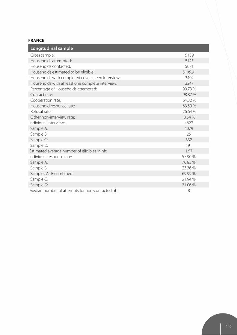
149
FRANCE
Longitudinal sampleGross sample: 5139Households attempted: 5125Households contacted: 5081Households estimated to be eligible: 5105.91Households with completed coverscreen interview: 3402Households with at least one complete interview: 3247Percentage of Households attempted: 99.73 %Contact rate: 98.87 %Cooperation rate: 64.32 %Household response rate: 63.59 %Refusal rate: 26.64 %Other non-interview rate: 8.64 %
Individual interviews: 4627 Sample A: 4079 Sample B: 25 Sample C: 332 Sample D: 191Estimated average number of eligibles in hh: 1.57Individual response rate: 57.90 % Sample A: 70.85 % Sample B: 23.36 % Samples A+B combined: 69.99 % Sample C: 21.94 % Sample D: 31.06 %Median number of attempts for non-contacted hh: 8

150
ISRAEL
Baseline / refreshment sampleGross sample: 701Households attempted: 537Households contacted: 501Households estimated to be eligible: 678.81Households with completed coverscreen interview: 362Households with at least one complete interview: 352Percentage of Households attempted: 76.60 %Contact rate: 71.30 %Cooperation rate: 72.73 %Household response rate: 51.86 %Refusal rate: 16.65 %Other non-interview rate: 2.80 %Individual interviews: 533Estimated average number of eligibles in hh: 1.77Individual response rate: 44.46 %Median number of attempts for non-contacted hh: 2
Longitudinal sampleGross sample: 1898Households attempted: 1729Households contacted: 1693Households estimated to be eligible: 1888.12Households with completed coverscreen interview: 1483Households with at least one complete interview: 1480Percentage of Households attempted: 91.10 %Contact rate: 89.19 %Cooperation rate: 87.89 %Household response rate: 78.38 %Refusal rate: 8.16 %Other non-interview rate: 2.65 %Individual interviews: 2287 Sample A: 1994 Sample B: 53 Sample C: 170 Sample D: 70Estimated average number of eligibles in hh: 1.67Individual response rate: 72.45 % Sample A: 82.33 % Sample B: 52.48 % Samples A+B combined: 81.13 % Sample C: 38.81 % Sample D: 35.53 %Median number of attempts for non-contacted hh: 2

151
ITALY
Baseline / refreshment sampleGross sample: 3100Households attempted: 3098Households contacted: 3053Households estimated to be eligible: 2631.70Households with completed coverscreen interview: 1231Households with at least one complete interview: 1144Percentage of Households attempted: 99.94 %Contact rate: 98.23 %Cooperation rate: 44.26 %Household response rate: 43.47 %Refusal rate: 50.50 %Other non-interview rate: 4.26 %Individual interviews: 1711Estimated average number of eligibles in hh: 1.60Individual response rate: 40.52 %Median number of attempts for non-contacted hh: 2
Longitudinal sampleGross sample: 2776Households attempted: 2766Households contacted: 2741Households estimated to be eligible: 2756.93Households with completed coverscreen interview: 1988Households with at least one complete interview: 1942Percentage of Households attempted: 99.64 %Contact rate: 98.73 %Cooperation rate: 71.34 %Household response rate: 70.44 %Refusal rate: 21.15 %Other non-interview rate: 7.15 %Individual interviews: 3202 Sample A: 2729 Sample B: 43 Sample C: 295 Sample D: 135Estimated average number of eligibles in hh: 1.71Individual response rate: 67.93 % Sample A: 81.22 % Sample B: 61.43 % Samples A+B combined: 80.82 % Sample C: 33.00 % Sample D: 34.62 %Median number of attempts for non-contacted hh: 5

152
LUxEMBOURG
Baseline / refreshment sampleGross sample: 4200Households attempted: 4186Households contacted: 4006Households estimated to be eligible: 3730.43Households with completed coverscreen interview: 1373Households with at least one complete interview: 1213Percentage of Households attempted: 99.67 %Contact rate: 94.84 %Cooperation rate: 34.28 %Household response rate: 32.52 %Refusal rate: 59.27 %Other non-interview rate: 3.06 %Individual interviews: 1606Estimated average number of eligibles in hh: 1.69Individual response rate: 25.49 %Median number of attempts for non-contacted hh: 3

153
NETHERLANDS
Baseline / refreshment sampleGross sample: 2697Households attempted: 2647Households contacted: 2527Households estimated to be eligible: 2520.73Households with completed coverscreen interview: 1261Households with at least one complete interview: 1229Percentage of Households attempted: 98.15 %Contact rate: 93.39 %Cooperation rate: 52.21 %Household response rate: 48.76 %Refusal rate: 41.54 %Other non-interview rate: 3.09 %Individual interviews: 1686Estimated average number of eligibles in hh: 1.67Individual response rate: 40.00 %Median number of attempts for non-contacted hh: 3
Longitudinal sampleGross sample: 2778Households attempted: 2628Households contacted: 2575Households estimated to be eligible: 2766.37Households with completed coverscreen interview: 1764Households with at least one complete interview: 1729Percentage of Households attempted: 94.60 %Contact rate: 92.68 %Cooperation rate: 67.43 %Household response rate: 62.50 %Refusal rate: 23.60 %Other non-interview rate: 6.58 %Individual interviews: 2560 Sample A: 2312 Sample B: 32 Sample C: 151 Sample D: 65Estimated average number of eligibles in hh: 1.70Individual response rate: 54.54 % Sample A: 83.14 % Sample B: 19.88 % Samples A+B combined: 79.67 % Sample C: 11.39 % Sample D: 15.29 %Median number of attempts for non-contacted hh: 2

154
SWEDEN
Baseline / refreshment sampleGross sample: 5000Households attempted: 4989Households contacted: 4759Households estimated to be eligible: 4609.14Households with completed coverscreen interview: 1924Households with at least one complete interview: 1810Percentage of Households attempted: 99.78 %Contact rate: 94.79 %Cooperation rate: 41.43 %Household response rate: 39.27 %Refusal rate: 51.94 %Other non-interview rate: 3.58 %Individual interviews: 2586Estimated average number of eligibles in hh: 1.68Individual response rate: 33.34 %Median number of attempts for non-contacted hh: 6
Longitudinal sampleGross sample: 2272Households attempted: 2253Households contacted: 2232Households estimated to be eligible: 2263.93Households with completed coverscreen interview: 1564Households with at least one complete interview: 1520Percentage of Households attempted: 99.16 %Contact rate: 98.24 %Cooperation rate: 68.35 %Household response rate: 67.14 %Refusal rate: 28.45 %Other non-interview rate: 2.65 %Individual interviews: 2154 Sample A: 1549 Sample B: 47 Sample C: 497 Sample D: 61Estimated average number of eligibles in hh: 1.61Individual response rate: 59.21 % Sample A: 79.07 % Sample B: 40.87 % Samples A+B combined: 76.95 % Sample C: 40.67 % Sample D: 17.84 %Median number of attempts for non-contacted hh: 14

155
SLOVENIA
Baseline / refreshment sampleGross sample: 1500Households attempted: 1339Households contacted: 1230Households estimated to be eligible: 1418.22Households with completed coverscreen interview: 598Households with at least one complete interview: 582Percentage of Households attempted: 89.27 %Contact rate: 81.58 %Cooperation rate: 50.30 %Household response rate: 41.04 %Refusal rate: 38.22 %Other non-interview rate: 2.33 %Individual interviews: 747Estimated average number of eligibles in hh: 1.62Individual response rate: 32.47 %Median number of attempts for non-contacted hh: 2
Longitudinal sampleGross sample: 2124Households attempted: 2100Households contacted: 2082Households estimated to be eligible: 2119.95Households with completed coverscreen interview: 1635Households with at least one complete interview: 1622Percentage of Households attempted: 98.87 %Contact rate: 98.02 %Cooperation rate: 78.06 %Household response rate: 76.51 %Refusal rate: 18.87 %Other non-interview rate: 2.64 %Individual interviews: 2262 Sample A: 2014 Sample B: 0 Sample C: 0 Sample D: 248Estimated average number of eligibles in hh: 1.66Individual response rate: 64.32 % Sample A: 73.53 % Sample B: . Samples A+B combined: 73.53 % Sample C: . Sample D: 31.88 %Median number of attempts for non-contacted hh: 2

156
Appendix 2: Number of released interviews by sample and country
Released interviews
Country SampleWave 1(2.6.0)
Wave 2(2.6.0)
Wave 3(1)
Wave 4(1.1.1)
Wave5(0)
Austria2004 1594 1228 885 854 810
2010 4478 3600
Belgium
2004 3827 2935 2723 2270 2062
2006 270 211 161 145
2010 2957 2134
2012 1391
Switzerland
2004 1004 752 662 582 482
2006 724 659 609 501
2010 2595 2084
Czech Republic
2006 2830 1938 1460 1295
2010 4736 3222
2012 1368
Germany
2004 3008 1715 1391 1169 824
2006 899 528 449 327
2012 4496
Denmark
2004 1707 1352 1168 1043 1003
2006 1314 1064 913 938
2010 437 386
2012 1926
Estonia 2010 6828 6044
Spain
2004 2396 1880 1842 1635 1598
2006 435 336 279 281
2010 1776 1484
Spanish region of Girona
2012 3283
France
2004 3193 2107 1895 1746 1456
2006 914 700 604 472
2010 3604 2614
Greece2004 2898 2360 2313
2006 932 786

157
Appendix 2: Number of released interviews by sample and country (continued)
Released interviews
Country SampleWave 1(2.6.0)
Wave 2(2.6.0)
Wave 3(1)
Wave 4(1.1.1)
Wave5(0)
Hungary 2010 3076
Ireland 2006 1134
Israel
2004 2598 2253 1713
2006 395 289
2012 555
Italy
2004 2559 2038 1861 1621 1644
2006 1001 722 610 570
2010 1442 918
2012 1710
Luxmbourg 2012 1610
Netherlands
2004 2979 1946 1760 1570 1419
2006 764 529 483 465
2010 769 621
2012 1670
Poland 2006 2467 2012 1880
Portugal 2010 2080
Sweden
2004 3053 2268 1830 1753 1740
2006 534 160 369 350
2012 2581
Slovenia2010 2756 2157
2012 724
Total 30816 37447 27975 59594 66962

158
9 Access to SHARE data and citation rulesDaniel Schmidutz, Munich Center for the Economics of Aging (MEA) at the Max Planck Institute for Social Law and Social Policy (MPISOC)
9.1 Availability of data sets
The Survey of Health, Ageing and Retirement in Europe (SHARE) covers 19 European countries and Israel in total. To date, SHARE has released data from five waves (2004/05, 2006/07, 2008/09, 2010/11, 2013) comprising more than 220.000 interviews of about 110.000 individuals aged 50 or over. Most recently, the data of the fifth wave of SHARE – consisting of more than 65.000 interviews – including its comprehensive documentation was released in March 2015.
In order to enable a permanent identification and reliable citability of the SHARE data in the digital environment, SHARE has been registered with a DOI name in 2013. The registration of each SHARE data set with a persistent Digital Object Identifier (DOI) improves the accessibility of the digital research data in terms of findability and traceability.
Currently, the following up-to-date data sets of the SHARE waves are available in Stata and SPSS format (either as full data sets or by modules):
• Wave 1: Release 2.6.0, November 29th 2013, DOI: 10.6103/SHARE.w1.260• Wave 2: Release 2.6.0, November 29th 2013, DOI: 10.6103/SHARE.w2.260• Wave 3 (SHARELIFE): Release 1.0.0, Nov. 24th 2010, DOI: 10.6103/SHARE.w3.100• Wave 4: Release 1.1.1, March 28th 2013, DOI:10.6103/SHARE.w4.111• Wave 5: Release 1.0.0, March 31st 2015, DOI: 10.6103/SHARE.w5.100
Besides, the following additional data sets have been released:
• easySHARE: Release 2.0.0, July 15th 2015, DOI: 10.6103/SHARE.easy.200• Job Episodes Panel: Release 2.0.0, August 13th 2014, DOI: 10.6103/SHARE.jep.200• SHARE-RV: Release 3.0.0, March 31st 2015, DOI: 10.6103/SHARE.SHARE-RV.300
easySHARE is a simplified HRS-adapted data set for student training and teaching, and for resear-chers who have little experience in quantitative analyses of complex survey data. It is stored as a long format panel data set and covers a subset of variables on all respondents of the released waves1 in one single data set, which is available in Stata, SPSS and R format. The Job Episodes Panel is a ready-to-use long format panel data set that identifies the labour market status of each SHARE respondent throug-hout her/his life. This data set rearranges information taken from Wave 1 to Wave 3 and can be easily in-tegrated with other information from SHARE or contextual and institutional information. The SHARE-RV data set refers to a German subsample of SHARE respondents and is composed of administrative data provided by the German Pension Fund (Deutsche Rentenversicherung) upon respondents‘ consent. It can easily be linked to the SHARE interviews of the same persons.
1 At the time of writing, a subset of variables from SHARE Waves 1, 2, 3 (SHARELIFE), 4, 5 are covered.

159
2 GESIS is a member of CESSDA (the Council of European Social Science Data Archives), another research infrastructure of the European Strategy Forum for Research Infrastructures (ESFRI) roadmap.
All SHARE data (except for the SHARE-RV data set, see details on data access below) are distributed through the SHARE Research Data Center (FDZ-SHARE), which complies with the Criteria of the German Council for Social and Economic Data (Rat für Sozial- und Wirtschaftsdaten, RatSWD) for providing ac-cess to microdata. Access to the data collected and generated in the SHARE projects is provided free of charge to all scientists globally, subject to European Union and national data protection laws. The trans-national, web-based access services are rendered through two public data archives in cooperation with the central SHARE coordination team at the Munich Center for the Economics of Aging (MEA) at the Max Planck Institute for Social Law and Social Policy (MPISOC): the CentERdata Archive located at Tilburg University in the Netherlands and the Data Archive for the Social Sciences (the former German Central Data Archive), a public data archive run by GESIS Leibniz-Institute for Social Sciences2 in Cologne.
9.2 Access to SHARE data and conditions of use
In accordance with the philosophy of sharing the data as soon as possible with the entire scientific community, a release policy has been adopted that gives free, quick and convenient access to all scien-tific users world-wide. The SHARE data may be used for scientific research without any restrictions as to specific research questions, subject to European Union and national data confidentiality rules (acknow-ledged by signature prior to access), and are most easily accessible via the SHARE Research Data Center homepage (cdata28.uvt.nl/sharedatadissemination/users/login). Eligible applicants have to take only three easy steps in order to obtain access to the SHARE data:
• Step 1: The applicant first requests access to the data by submitting a completed and signed user statement on data confidentiality through e-mail, fax, or postal mail. In this „Statement concerning the use of SHARE data“ the applicant provides credentials that s/he is affiliated with a scientific institution. The latest version of the respective form can be easily downloaded from the project‘s website:
www.share-project.org/fileadmin/pdf_documentation/SHARE_Data_Statement.pdf
Data will only be made available after this document has been received.
• Step 2: Upon acceptance of the credentials (normally within a few working days), access will be granted to the SHARE Research Data Center website via a personal user ID and a password.
• Step 3: Finally, the SHARE data can be downloaded by the user from the SHARE Research Data Center. Registered users of the data are regularly informed about updates of data and new releases via e-mail. Regarding the subsequent use of the data, users are supported by a public website providing various information and by a combination of central and national support points which answer questions and respond to user requests.
Access to the data is subject to the following SHARE Data Access Rules and Conditions of Use, which are publicly available in their most recent version on the project‘s website:
www.share-project.org/data-access-documentation/research-data-center-data-access.html

160
It is obligatory for all users to fill out and sign the “Statement concerning the use of SHARE data“. In the statement, users have to assure that they will use the data for scientific research purposes only – this is very important, as any commercial use of the SHARE data is strictly prohibited. To guarantee the pu-rely scientific use of the data users are obliged to indicate their scientific affiliation (university, research institute, public policy institute). As part of this declaration, all users commit themselves not to make any copies of the data available to others or enable any third party access to the database. Furthermore, the statement also includes a self-commitment of the individual user to take no action aiming at a re-identification of participants of the study. All non-EU users are obliged to sign the very same declaration, binding them to EU data protection laws.
Access to the SHARE data is granted on an individual basis only. Each person working on a scientific project or publication using SHARE data has to fill out and sign the “Statement concerning the use of SHARE data“ individually. Registered users are allowed to use data of the SHARE project as long as the scientific affiliation indicated in the user statement is valid. The original login code and password persist for all subsequent releases of the data. A new statement has to be submitted, however, when any of the specifications given in the statement (including the e-mail address) change.
Finally, further conditions of use concern the obligation to provide information about publications, the acknowledgement of data collection and of main funding institutions and the implementation of SHARE citation practices. First, users are requested to provide references to all publications and pa-pers based on SHARE data to the central SHARE coordination team. Second, whenever a publication is produced or a paper is written using SHARE data, the SHARE data set/s used (including the respective DOI/s) must be referred to and the funding sources have to be acknowledged (the acknowledgement referring to the up-to-date data sets may be viewed on the project‘s website; please see the citation rules in chapter 9.3 for the current version of the acknowledgements). Third, besides citing the used data set/s, users are requested to read and then include the basic literature on SHARE research and methodology in the bibliography corresponding to the data set/s they have used in the paper, which are specified on the respective subpage of each wave on the project‘s website (www.share-project.org; please also refer to the SHARE citation rules in chapter 9.3).
Concerning the above mentioned additional data sets with a SHARE-related DOI, application and access procedures vary with respect to the easySHARE data set and the SHARE-RV data set.
As regards the easySHARE data set, a simplified application procedure may be used by registered users who want to use easySHARE for teaching purposes. This simplified application procedure allows the instructors to distribute the easySHARE data set to the participants of their course/s by filling out and signing the “easySHARE teacher statement“ and provides a convenient way of registering all course participants as regular SHARE users at the same time. The “easySHARE teacher statement“ form can be easily downloaded from the project‘s website:
www.share-project.org/fileadmin/pdf_documentation/easySHARE_Teacher_Statement.pdf
3 At the time of writing, the SHARE coordination team is looking into possibilities under which access to SHARE data will also be possible if applicants without an affiliation to a university or research institute demonstrate the scientific purpose and nature of the envisaged research project in a sufficient manner.

161
and is included in the data download zip file. Since the easySHARE data set is composed of data from the released SHARE waves the SHARE Data Access Rules and Conditions of Use described above also apply to the easySHARE data set.
Regarding the SHARE-RV data set an additional application has to be submitted to the Research Data Center of the German Pension Fund (FDZ-RV). Following a successful registration (via the website of the FDZ-RV) the data set will be provided to researchers on a compact disc free of charge. After regis-tration as a regular SHARE user, following the procedure and subject to the conditions described above, the administrative data can easily be linked with the German SHARE survey data via the identification numbers contained in the data set, which is identical with the identification numbers used in the re-leased SHARE data sets. Further details regarding SHARE-RV, including detailed information on how to obtain access to the data set, are available on the project‘s website:
www.share-project.org/data-access-documentation/record-linkage-share-rv.html
9.3 SHARE citation rules
By signing the SHARE user statement users agree to include an acknowledgement containing the following information in all their publications using SHARE data:
This paper uses data from SHARE Waves 1, 2, 3 (SHARELIFE), 4 and 5 (DOIs: 10.6103/SHARE.w1.260, 10.6103/SHARE.w2.260, 10.6103/SHARE.w3.100, 10.6103/SHARE.w4.111, 10.6103/SHARE.w5.100), see Börsch-Supan et al. (2013) for methodological details4.
The SHARE data collection has been primarily funded by the European Commission through FP5 (QLK6-CT-2001-00360), FP6 (SHARE-I3: RII-CT-2006-062193, COMPARE: CIT5-CT-2005-028857, SHARE-LIFE: CIT4-CT-2006-028812) and FP7 (SHARE-PREP: N°211909, SHARE-LEAP: N°227822, SHARE M4: N°261982). Additional funding from the German Ministry of Education and Research, the U.S. Na-tional Institute on Aging (U01_AG09740-13S2, P01_AG005842, P01_AG08291, P30_AG12815, R21_AG025169, Y1-AG-4553-01, IAG_BSR06-11, OGHA_04-064) and from various national funding sour-ces is gratefully acknowledged (see www.share-project.org).
easySHARE is intended for student training and teaching purposes. For scientific publications it is recommended to use the main data set of SHARE, or to carefully study the easySHARE documentation and the Stata program that extracts and generates easySHARE from the main release of SHARE. In case easySHARE data is being used for theses or other scientific publications, the following additional ack-nowledgement has to be included:
4 Usually this information will be part of the text of a scientific publication already. If this is the case, there is no need to include this information in the acknowledgement once more.

162
This paper uses data from the generated easySHARE data set (DOI: 10.6103/SHARE.easy.200), see Gruber et al. (2014) for methodological details. The easySHARE release 2.0.0 is based on SHARE Waves 1, 2, 3 (SHARELIFE), 4 and 5 (DOIs: 10.6103/SHARE.w1.260, 10.6103/SHARE.w2.260, 10.6103/SHARE.w3.100, 10.6103/SHARE.w4.111, 10.6103/SHARE.w5.100). 4
The following additional acknowledgement has to be included when publishing with SHARE Job Episodes Panel data:
This paper uses data from the generated Job Episodes Panel (DOI: 10.6103/SHARE.jep.200), see Brugiavini et al. (2013) and Antonova et al. (2014) for methodological details. The Job Episodes Panel release 2.0.0 is based on SHARE Waves 1 and 2 (release 2.5.0, May 24th 2011) and SHARELIFE (DOI: 10.6103/SHARE.w3.100).4
In line with the general SHARE acknowledgement, when using any SHARE data, it is mandatory for users to cite the following publication in addition to the SHARE respective acknowledgement/s:
Börsch-Supan, A., M. Brandt, C. Hunkler, T. Kneip, J. Korbmacher, F. Malter, B. Schaan, S. Stuck, S. Zuber (2013). Data Resource Profile: The Survey of Health, Ageing and Retirement in Europe (SHARE). Inter-national Journal of Epidemiology. DOI: 10.1093/ije/dyt088
When using easySHARE or Job Episode Panel data, in line with the respective additional acknowledge-ments, users are required to cite the following publications:
easySHARE: Gruber, S., C. Hunkler and S. Stuck (2014). Generating easySHARE: guidelines, structure, content and programming. SHARE Working Paper Series: 17-2014. Munich: MEA, Max Planck Institute for Social Law and Social Policy.
Job Episodes Panel: Antonova, L., L. Aranda, G. Pasini and E. Trevisan (2014). Migration, family history and pension: the second release of the SHARE Job Episodes Panel. SHARE Working Paper Series: 18-2014. Munich: MEA, Max Planck Institute for Social Law and Social Policy.
Brugiavini, A., D. Cavapozzi, G. Pasini and E. Trevisan (2013). Working life histories from SHARELIFE: a retrospective panel. SHARE Working Paper Series: 11-2013. Munich: MEA, Max Planck Institute for Social Law and Social Policy.

163
Furthermore, SHARE provides wave specific methodological documentation of the data which should be referenced for data description purposes in any publication using data from the respective wave:
Wave 1: Börsch-Supan, A. and H. Jürges (Eds.) (2005). The Survey of Health, Ageing and Retirement in Europe – Methodology. Mannheim: Mannheim Research Institute for the Economics of Aging (MEA).
Wave 2: Börsch-Supan, A., A. Brugiavini, H. Jürges, A. Kapteyn, J. Mackenbach, J. Siegrist, G. Weber (Eds.) (2008). First results from the Survey of Health, Ageing and Retirement in Europe (2004-2007). Starting the longitudinal dimension. Mannheim: Mannheim Research Institute for the Economics of Aging (MEA).
Wave 3: Schröder, M. (Ed.) (2011). Retrospective data collection in the Survey of Health, Ageing and Retirement in Europe. SHARELIFE methodology. Mannheim: Mannheim Research Institute for the Economics of Aging (MEA). Wave 4: Malter, F. and A. Börsch-Supan (Eds.) (2013). SHARE Wave 4: Innovations & Methodology. Munich: MEA, Max Planck Institute for Social Law and Social Policy.
Wave 5: Malter, F. and A. Börsch-Supan (Eds.) (2015). SHARE Wave 5: Innovations & Methodology. Munich: MEA, Max Planck Institute for Social Law and Social Policy.
SHARE accompanies every newly released wave with a volume on first, preliminary findings (“First Results Book“). Their citation is recommended when referring to substantial findings generated on the basis of SHARE data:
Börsch-Supan, A., A. Brugiavini, H. Jürges, J. Mackenbach, J. Siegrist, G. Weber (Eds.) (2005). Health, ageing and retirement in Europe – First results from the Survey of Health, Ageing and Retirement in Europe. Mannheim: Mannheim Research Institute for the Economics of Aging (MEA).
Börsch-Supan, A., M. Brandt, K. Hank, M. Schröder (Eds.) (2011). The individual and the welfare state. Life histories in Europe. Heidelberg: Springer.
Börsch-Supan A., M. Brandt , H. Litwin, G. Weber (Eds.) (2013). Active ageing and solidarity between generations in Europe: First results from SHARE after the economic crisis. Berlin: De Gruyter.

164
Finally, it is mandatory to cite the respective data set(s) used for the publication. As there are no gene-ral data citation standards for data sets yet, a citation based on the da|ra metadata schema (Hausstein et al. 2014) is recommended, which is also in line with the recommended standard according to DataCite (c.f. DataCite Metadata Working Group 2013):
Börsch-Supan, A. (2013). Survey of Health, Ageing and Retirement in Europe (SHARE) Wave 1. Release version: 2.6.0. SHARE-ERIC. Data set. DOI: 10.6103/SHARE.w1.260
Börsch-Supan, A. (2013). Survey of Health, Ageing and Retirement in Europe (SHARE) Wave 2. Release version: 2.6.0. SHARE-ERIC. Data set. DOI: 10.6103/SHARE.w2.260
Börsch-Supan, A. (2010). Survey of Health, Ageing and Retirement in Europe (SHARE) Wave 3 – SHARELIFE. Release version: 1.0.0. SHARE-ERIC. Data set. DOI: 10.6103/SHARE.w3.100
Börsch-Supan, A. (2013). Survey of Health, Ageing and Retirement in Europe (SHARE) Wave 4. Release version: 1.1.1. SHARE-ERIC. Data set. DOI: 10.6103/SHARE.w4.111
Börsch-Supan, A. (2015). Survey of Health, Ageing and Retirement in Europe (SHARE) Wave 5. Release version: 1.0.0. SHARE-ERIC. Data set. DOI: 10.6103/SHARE.w5.100
Börsch-Supan, A., C. Hunkler, S. Gruber, A. Orban, S. Stuck, M. Brandt (2015). easySHARE. Release version: 1.0.0. SHARE-ERIC. Data set DOI: 10.6103/SHARE.easy.200
Antonova, L., L. Aranda, A. Brugiavini, D. Cavapozzi, G. Pasini, E. Trevisan (2014). SHARE Job Episodes Panel. Release version: 2.0.0. SHARE-ERIC. Data set. DOI: 10.6103/SHARE.jep.200
Forschungsdatenzentrum der Rentenversicherung, Max-Planck-Institut für Sozialrecht und Sozialpo-litik (2015). SHARE-RV. Release version: 3.0.0. SHARE-ERIC. Data set. DOI: 10.6103/SHARE.SHARE-RV.300
ReferencesHausstein, B., Schleinstein, N., Koch, U. , Meichsner, J., Becker, K. & Stahn, L.-L. (2014). da|ra Metadata Schema. Version: 3.0. GESIS Leibniz Institute for the Social Sciences. DOI: 10.4232/10.mdsdoc.3.0.
DataCite Metadata Working Group (2013). DataCite Metadata Schema for the Publication and Citation of Research Data. Version 3.1. DataCite. Text. DOI:10.5438/0008.

165
10 Measuring interview length with keystroke dataJohanna Bristle, Munich Center for the Economics of Aging (MEA) at the Max Planck Institute for Social Law and Social Policy (MPISOC)
10.1 Introduction
In SHARE, interviewers conduct interviews by using laptops where the respondents’ answers are being entered right away. The computer-assisted mode allows the collection of process information as a by-product while the interview is being administered. Data that are captured during the process of survey data collection and which provide “information about the data collection process on a […] micro-level” (Kreuter, 2013, p. 3) are called “paradata”. One type of paradata is keystroke data. Keystrokes are records of every action on a laptop’s keyboard, i.e. they allow for a very detailed reconstruction of what the interviewer entered at what point in time as the software logs a time stamp every time a key is pressed. In this chapter, keystroke data is used to calculate durations of SHARE interviews.
The intention of this chapter is twofold: firstly, it provides documentation on how keystroke data in SHARE were collected and prepared (for details see chapter 2.1). This can guide interested researchers employed by SHARE in understanding and analysing keystroke data. Secondly, it describes the length of SHARE interviews in Wave 5 by different subgroups, in comparison to the previous wave and from a cross-national perspective. Total interview length estimates are computed comparably to length es-timates of Wave 1 (cf. Jürges 2005). In addition, it documents interview durations by subgroups for all participating countries separately in the Appendix.
10.2 keystroke data in SHARE
While the survey interview was conducted using Blaise software, keystroke data were collected by means of tracking audit trails1. Every action taken on the keyboard of the laptop was registered and stored by Blaise in a text file. Figure 10.1 shows the response options in the CAPI instrument to the ques-tion “During the past twelve months, how often did you have contact with your father, either in person, by phone, mail, email or any other electronic means?”. The section where the CAPI instrument stored the answers (example DN032, which refers to the question text above, highlighted in red) was displayed at the bottom of the window. The place where the answer was stored is called a “field”. The corresponding data excerpt is displayed in Figure 10.2. In the example highlighted in red, the interviewer selected the answer using the mouse, pressed ENTER (“Key: 13”), and then the answer was stored. The text file con-tained information on the time of entry into a field, exit out of a field, and all actions in between (enter-ing of an answer, editing the answer, opening additional screens like a help file, or mouse movements). Time stamps were attached to every action.
1 Audit trails track system activity and provide a way to observe the interaction between the computer system and the user (here: the interviewer). Strictly, the information of the field that is entered is no keystroke information but it helps to identify the location in the questionnaire.

166
From these text files, durations on field level were computed by CentERdata and saved as STATA and SPSS files. Besides the time spent on a field, the following information was recorded: the name of the field (which contained the item number of the questionnaire), the answer of the respondent, if the interview was restarted, the number of times an item was accessed, backed-up, if a remark was set, and the remark itself. To link keystroke data and survey data, respondent and laptop identifiers were extracted.
Figure 10.1: Screenshot of item DN032 in CAPI instrument
Figure 10.2: Screenshot of of keystroke data

167
Figure 10.3 shows a snapshot of this extraction. For example, the field that corresponded to item DN032 was activated for 11 seconds (stored in the variable secfield).
The structure of the Wave 5 data was rather complex. Information was stored on field-level with one observation in the data per screen that was shown during the interview. A field referred to one item in the CAPI questionnaire. This resulted in a hierarchical structure of the data: fields were nested within interviews, which were nested within laptops, which were then nested within survey agencies. It also resulted in a non-rectangular structure of the data, which means that the number of observations varied over respondents. The reason is that respondents received different numbers of questions due to routing.
Keystroke data in SHARE Wave 5 were aggregated at the analysis level of interest, e.g. item, module, or respondent level. The respondent level2 file became part of an internal paradata set and was stored as a generated variable module (gv_ks). ID corrections were made in accordance to the SHARE survey data to be compatible with the release data. The gv_ks module includes variables on the length of interview and the number of items asked throughout the entire interview. It also includes the duration and the number of items asked for each module in the main questionnaire. In case of an early termination of the interview, a variable indicates at which module the termination occurred. The questionnaire contained introduction texts to modules or topics to be read-out by the interviewer. The durations of some of these items were included in the gv_ks for investigating interviewer behaviour.
Figure 10.3: Screenshot of selected variables on field-level
2 The level of aggregation depends on the analytical purpose. Keystroke data are valuable during all phases of the survey lifecycle - before fieldwork for informing questionnaire development, during fieldwork for investigating interviewer behaviour and post fieldwork for data quality analysis. Examples for these various analytical purposes based on SHARE’s keystroke data and time stamp data from the European Social Survey (ESS) can be found in Bristle, J. and V. Halbherr (2014). Keystroke Analysis and Implications for Fieldwork. DASISH, Work Package 3, Deliverable D3.7. Retrieved from http://dasish.eu/deliverables/.

168
Figure 10.4: Conceptual measurement of interview length
10.3 Measuring interview length
When using keystroke data we attempt to measure the pure length of the CAPI interview. However, the theoretical concept of interview length is ambiguous and depends on the perspective of the re-spective actor in a survey. What a respondent means when asking “How long will it take” is conceptu-ally different from what questionnaire designer estimate. Questionnaire design often follows a rule of thumb, which is “four ticks per minute” (Jürges 2005) or in other words, four responses can be given per minute. In face-to-face interviews, the respondent might include the total time an interviewer spends at the household, which might include small talk. This process is depicted in Figure 10.4.
In SHARE the interview consisted of a household coverscreen, at least one individual CAPI interview (mostly one or two), and sometimes a self-completion questionnaire (drop-off ). Keystrokes only measu-red the length of the CAPI interview(s). Furthermore, the interview length was shaped to a large extent by respondent- and interviewer-specific characteristics.
Generally, interview length can either be calculated by subtracting the time stamp at the beginning of the interview from the time stamp at the end of the interview, or by computing the sum of all item durations derived from keystroke data. With keystroke data of Wave 5 it was possible to correct duration measures (e.g. outliers) on item-level. This was of particular importance towards the end of the inter-view when the interviewer section started (IV module). The interviewer answered a few questions about the interview process without the respondent’s participation. Sometimes keystroke data showed very long durations at the start of this last module, indicating that the interviewer left the respondent and completed this last module later. Keystroke data allowed for more accurate measurement of the actual interview time than simply looking at the time stamps that indicate beginning and end of the interview.
A rather conservative approach was adopted to deal with outliers. Only cases which were caused by a technical error or which were so high that the interview seemed interrupted were dropped. Thresholds for plausible values were set at a fixed value, and not according to the statistical distribution. This is an adequate rule for the requirements of fieldwork management. All Wave 5 items over 1,000 seconds

169
were set to missing except items in modules that were expected to last long (grip strength measure-ment and asking for record linkage). Here, durations exceeding the threshold were truncated at 1000 seconds (roughly 15 minutes). Furthermore, we set a minimum fixed threshold of 1 second. Durations of zero seconds and negative values were set to missing3 .
As a panel study, SHARE’s main concern in questionnaire design was finding a balance between keeping the longitudinal dimension on the one hand, and improving or adding measures of substantial interest to the research community on the other hand. Changes in the questionnaire content often resulted in changes in interview length. They were monitored with the overall goal of not making the interview longer over waves. Longer interviews impose a larger burden on the respondents; therefore respondents might in general be less willing to participate in a survey that takes long (Bradburn, 1978). Galesic and Bosnjak (2009) randomly varied the stated interview length in a web survey and found that more respondents started and completed the questionnaire if the stated interview length was short. Looking at the longitudinal dimension, evidence is less clear with results showing that there is no ef-fect of length on attrition (Lynn, 2013) and others showing a positive correlation between length and participation in a later wave of a panel (Fricker et al., 2012; Bristle et al., 2014). While the stated length seems to matter for first-time participation, respondents seem to make their decision to re-participate in a survey based on other factors than length alone. More importantly, interview length should be part of monitoring data quality. Respondent’s concentration and motivation weakens over the course of an interview. This might result in more ‘satisficing’ or ‘straight-lining’ behaviour and reduced data quality (Krosnick, 1991). Empirical evidence shows that towards the end of the questionnaire, response latenci-es become shorter and item nonresponse increases (Galesic and Bosnjak, 2009). Respondents of shorter interviews reported the interview to be less burdensome. In addition, longer interviews are more ex-pensive than shorter ones regarding the payment of the interviewer (Jürges, 2005).
10.4 Length by subgroups
In Figure 10.5 the interview length of Wave 5 is presented separately for six subgroups, which repre-sent the major differentiations of SHARE interviews4. Here we distinguish between panel vs. refreshment respondents and between the numbers of interviews conducted within one household. An interview in a single household in Wave 5 took about 76 minutes if the person was a first-time respondent and 66 minutes if the person participated again in the panel. Couple interviews consisted of two individual interviews. The first couple interview took on average 75 minutes for a refreshment household (plus 47 minutes for the second interview) and 64 plus 42 minutes for a panel household (see Figure 10.5 or Tab-le A1 in the appendix). It needs to be noted that in a couple interview the first interview was only slightly shorter than a single interview, while the second interview was much shorter. This was due to routing.
3 Some fields contained valid survey answers which were not necessarily answered during the survey but have been preloaded (e.g. a child’s first name or year of birth). The time spent on verifying the preloaded information was stored in the preceding question. For some other cases, inaccuracy in measurement might be a reason for zero seconds. The field durations were rounded to seconds and therefore could result in zero seconds although the field was activated for 0.3 seconds (as an example). The decision to keep or drop those cases depended on the underlying research question.4 Analyses were made based on the sample of Wave 5 release 0. The following further sample restrictions were applied: end-of-life interviews and nursing home interviews are excluded. Cases with missing keystroke information could not be conisdered. The sample is restricted to completed interviews (or at least completed until the grip strength module). All analyses are restricted to individual interviews of at least 20 minutes and 200 minutes most. Analyses on couple level only include couple interviews where both interviews were released and both were either longitudinal or refreshment (i.e. households with new spouses were dropped).

170
5 The analysis is made accordingly to Figure 10.5. Wave 4 data is based on the sample of release 1.1.1.
0
50
100
150
leng
th in
min
utes
REFRESHMENT PANEL
single couple-first couple-second single couple-first couple-second
excludes outside valuesData: Sample based on wave 5 release data.
Length by interview version - wave 5
Figure 10.5: Length by interview version in Wave 5
Figure 10.6: Comparison of interview length Wave 4 and Wave 5
10.5 Length over waves
Interview length of the current wave was compared to the length of the previous wave. The ultimate goal was not making the interview longer over waves. Looking at the development across waves, the interview length increased from Wave 4 to Wave 5 only for refreshment interviews5 (see Figure 10.6). In comparison to published results of Wave 1 (see Jürges, 2005), the refreshment interview for single inter-views stayed the same from Wave 1 to Wave 4 and then increased in Wave 5. For panel respondents, the interview length stayed roughly the same.

171
10.6 Length by country
In a cross-national survey, an obvious further level of comparison is the country. On the one hand, length variation can occur due to language and cultural differences. On the other hand, it might be partly due to differential strategies in survey management, training or interviewer behaviour. The latter are causes for variation which ought to be minimized in ex-ante harmonised, international data collec-tion. Interviewers play a very important role in face-to-face surveys. For example, in Slovenia and Israel a relatively low total number of interviewers conducted the SHARE study6. This means few interviewers had to make a lot of interviews. In this case it is especially important that the interviewers are trained to conduct the interviews in a standardized way. Otherwise a single interviewer’s non-standardized behaviour might affect a relatively large share of the sample.
The comparison of interview length across countries is reported below for the subgroup of sin-gle interviews; separately for refreshment (Figure 10.7) and panel respondents (Figure 10.8). In Wave 5, the longest average durations were reported for Luxembourg, Belgium-fr and Sweden, while the shortest average durations were found in Slovenia and Israel. The variation between countries was consistent across the panel dimension of SHARE. In Wave 1 analyses, “the shortest interviews were made in Austria, Spain, and Italy (…). The longest interviews were conducted in Denmark and Sweden” (Jürges, 2005, p. 83). This pattern was repeated in Wave 57.
6 In Slovenia, 48 interviewers worked for SHARE in Wave 5. In Israel, 21 interviewers were employed and worked on the sample of Wave 5.7 The only countries which showed shorter or longer durations in Wave 5 than in Wave 1 did not participate in Wave 1 (Luxemburg, Slovenia, Israel) or were not part of the Wave 1 keystroke analysis (Belgium).
0
50
100
150
200
leng
th in
min
utes
lu be_fr se de dk nl be_nl cz it si ilexcludes outside valuesData: Sample based on wave 5 release 0.
Length by Country (refreshment & single)
Figure 10.7: Length by country for subgroup „single refreshment interview“

172
0
50
100
150
leng
th in
min
utes
se be_fr de dk nl fr ch cz be_nl ee at es it il siexcludes outside valuesData: Sample based on wave 5 release 0.
Length by Country (panel & single)
Figure 10.8: Length by country for subgroup “single panel interview”
ReferencesBradburn, N.M. (1978). Respondent burden. Proceedings of the Survey Research Methods, Section of the American Statistical Association, pp. 35–40.
Bristle, J., Celidoni, M., Dal Bianco, C. & Weber, G. (2014). The contribution of paradata to panel cooperation in SHARE. SHARE Working Paper Series. Munich: Munich Center for the Economics of Aging (MEA).
Bristle, J. & Halbherr, V. (2014). Keystroke analysis and implications for fieldwork. DASISH, Work Package 3, Deliverable D3.7. Retrieved from http://dasish.eu/deliverables/.
Fricker, S., Creech, B., Davis, J., Gonzalez, J., Tan, L. & To, N. (2012). Does length really matter? Exploring the effects of a shorter interview on data quality, nonresponse, and respondent burden. Paper presented at the Federal Committee on Statistical Methodology 2012 Research Conference. Washington DC, USA.
Galesic, M. & Bosnjak, M. (2009). Effects of questionnaire length on participation and indicators of res-ponse quality in a web survey. Public Opinion Quarterly 73(2), pp. 349-36.
Jürges, H. (2005). Interview, module, and question length in SHARE. In: Börsch-Supan, A. & Jürges, H. (Eds.). The Survey of Health, Ageing and Retirement in Europe – Methodology, pp. 82-87. Mannheim: MEA.
Kreuter, F. (2013). Improving Surveys with Paradata. Introduction. In Kreuter, F. (Ed.) Improving Surveys with Paradata. Hoboken, New Jersey: John Wiley & Sons.
Krosnick, J.A. (1991). Response strategies for coping with the cognitive demands of attitude measures in surveys. Applied Cognitive Psychology. 5, pp. 213-236.
Lynn, P. (2013). Longer interviews may Not affect subsequent survey participation propensity. Under-standing Society Working Paper Series. 2013 - 07. Retrieved from https://www.understandingsociety.ac.uk/research/publications/working-paper/understanding-society/2013-07.pdf.

173
APPENDIx
Interview version Sample Mean Median SD Min Max N
Single Refreshment 79,41 75,90 29,39 20,07 197,97 4541
Single Panel 69,21 65,60 26,17 20,00 196,92 11871
Couple-first Refreshment 77,74 75,08 27,39 20,05 199,58 10069
Couple-first Panel 66,95 63,83 23,58 20,02 198,35 16671
Couple-second Refreshment 49,71 47,15 18,21 20,02 180,08 7565
Couple-second Panel 44,73 42,07 15,97 20,00 183,53 11523
Country Interview version Sample Mean Median SD Min Max N
AT
Single Refreshment 64,92 65,20 26,82 21,57 120,82 15
Single Panel 66,44 62,53 25,50 20,28 191,50 1371
Couple-first Refreshment 64,06 60,71 25,94 22,98 126,88 30
Couple-first Panel 62,45 59,57 22,04 20,07 183,13 1438
Couple-second Refreshment 45,23 42,27 16,54 20,57 104,12 119
Couple-second Panel 40,64 38,50 14,10 20,02 116,72 989
BE (fr)
Single Refreshment 93,12 90,67 29,14 31,05 167,10 221
Single Panel 81,75 77,52 27,24 27,98 196,62 677
Couple-first Refreshment 90,10 86,63 26,38 35,18 197,58 398
Couple-first Panel 78,75 74,80 23,83 20,78 196,02 738
Couple-second Refreshment 55,66 54,25 18,40 20,07 146,52 257
Couple-second Panel 49,96 46,68 17,50 20,43 158,70 436
BE (nl)
Single Refreshment 82,38 78,11 26,16 38,65 174,03 86
Single Panel 70,33 66,47 22,81 23,68 167,13 561
Couple-first Refreshment 77,11 72,33 22,63 38,48 156,65 276
Couple-first Panel 68,74 64,77 20,23 28,27 171,42 905
Couple-second Refreshment 46,66 44,90 15,94 21,25 132,10 201
Couple-second Panel 42,16 39,42 13,80 20,73 140,25 653
Table A1: Interview length Wave 5 by subgroups
Table A2: Interview length Wave 5 by subgroups and countries
Note: The sample was based on Wave 5 release 0. Further restrictions were applied (see Footnote 4). SD=standard deviation, N=Number of observations.

174
Table A2: Interview length Wave 5 by subgroups and countries (continued)
Country Interview version Sample Mean Median SD Min Max N
CH
Single Refreshment 74,67 74,33 31,42 34,82 112,05 6
Single Panel 73,00 69,92 24,78 20,57 172,27 691
Couple-first Refreshment 79,43 88,10 23,90 45,40 125,78 13
Couple-first Panel 71,15 68,39 23,56 20,72 196,00 1364
Couple-second Refreshment 54,88 52,33 20,04 20,07 118,57 79
Couple-second Panel 48,40 46,33 15,18 20,00 105,97 765
CZ
Single Refreshment 69,27 65,93 25,03 23,60 187,40 392
Single Panel 72,03 67,63 26,38 20,22 196,92 1306
Couple-first Refreshment 68,14 64,50 23,43 25,10 181,93 557
Couple-first Panel 69,29 64,87 24,53 20,65 195,02 1493
Couple-second Refreshment 45,20 42,28 16,27 20,17 127,63 524
Couple-second Panel 45,22 42,67 17,10 20,22 149,47 1179
DE
Single Refreshment 89,15 85,24 25,55 39,60 189,12 880
Single Panel 77,22 76,07 22,34 25,93 182,48 250
Couple-first Refreshment 87,50 84,67 23,50 32,45 197,52 2073
Couple-first Panel 77,06 75,00 20,46 36,32 169,12 486
Couple-second Refreshment 54,97 52,62 16,11 20,67 138,50 1496
Couple-second Panel 48,86 47,25 13,68 20,27 114,27 355
Dk
Single Refreshment 86,31 83,07 24,78 20,50 186,88 359
Single Panel 77,65 72,93 24,39 26,47 186,78 558
Couple-first Refreshment 81,32 79,12 20,71 27,10 167,88 923
Couple-first Panel 74,48 71,15 20,63 25,47 162,27 925
Couple-second Refreshment 51,02 49,25 13,40 24,37 102,00 649
Couple-second Panel 47,87 45,53 13,21 20,35 100,60 641
EE
Single Refreshment 113,36 113,36 78,45 57,88 168,83 2
Single Panel 68,73 64,13 27,48 20,13 187,97 1845
Couple-first Refreshment 76,07 67,68 28,48 40,20 144,00 33
Couple-first Panel 69,67 64,61 25,60 20,68 190,72 1880
Couple-second Refreshment 47,95 44,07 19,71 20,77 123,08 172
Couple-second Panel 44,75 41,16 17,72 20,02 161,45 1530
Note: The sample was based on Wave 5 release 0. Further restrictions were applied (see Footnote 4). SD=standard deviation, N=Number of observations.

175
Table A2: Interview length Wave 5 by subgroups and countries (continued)
Country Interview version Sample Mean Median SD Min Max N
ES
Single Refreshment 72,62 82,02 26,43 42,77 93,07 3
Single Panel 58,73 58,18 17,78 20,57 137,15 714
Couple-first Refreshment 64,81 65,89 15,99 25,70 94,37 22
Couple-first Panel 59,53 57,97 16,03 20,18 146,38 1186
Couple-second Refreshment 45,59 40,63 16,54 22,77 88,33 68
Couple-second Panel 45,26 43,61 14,28 20,03 118,67 990
FR
Single Refreshment 80,54 73,07 20,52 53,35 115,37 16
Single Panel 74,60 71,43 23,08 24,17 189,08 1360
Couple-first Refreshment 76,26 68,43 22,46 40,38 130,20 58
Couple-first Panel 71,94 68,43 21,44 24,25 188,17 1618
Couple-second Refreshment 54,58 52,40 16,41 20,92 106,75 131
Couple-second Panel 47,89 45,59 15,15 20,80 138,33 1142
IL
Single Refreshment 47,67 42,90 19,63 20,07 110,92 84
Single Panel 46,08 43,92 16,84 20,00 105,90 403
Couple-first Refreshment 41,66 38,19 16,64 20,05 170,85 282
Couple-first Panel 46,00 42,57 18,07 20,10 175,92 667
Couple-second Refreshment 34,45 31,60 11,00 20,35 76,73 175
Couple-second Panel 34,40 32,41 11,56 20,00 105,87 448
IT
Single Refreshment 67,16 61,65 28,96 20,07 180,92 430
Single Panel 55,97 53,22 20,25 20,45 164,07 587
Couple-first Refreshment 64,69 59,79 25,51 20,92 199,58 708
Couple-first Panel 57,62 55,60 18,48 20,85 154,32 1211
Couple-second Refreshment 45,09 39,52 23,16 20,02 180,08 619
Couple-second Panel 38,65 36,35 14,49 20,03 162,73 912
LU
Single Refreshment 95,67 92,00 31,09 25,65 195,02 323
Couple-first Refreshment 92,86 88,39 25,50 37,80 196,78 830
Couple-second Refreshment 57,20 54,28 20,32 22,17 161,27 392
Note: The sample was based on Wave 5 release 0. Further restrictions were applied (see Footnote 4). SD=standard deviation, N=Number of observations.

176
Country Interview version Sample Mean Median SD Min Max N
NL
Single Refreshment 83,81 80,36 26,22 20,20 177,50 372
Single Panel 75,80 72,92 24,51 24,60 149,17 511
Couple-first Refreshment 80,07 77,22 23,41 23,67 169,35 836
Couple-first Panel 72,00 70,54 20,01 21,33 150,73 1074
Couple-second Refreshment 50,22 47,39 15,95 20,33 116,47 496
Couple-second Panel 45,77 43,57 13,58 20,08 97,27 709
SE
Single Refreshment 91,24 87,47 28,21 23,83 197,97 554
Single Panel 86,86 83,23 26,81 21,95 190,12 524
Couple-first Refreshment 91,96 88,42 28,13 25,88 198,25 1247
Couple-first Panel 81,75 78,17 24,66 25,15 198,35 777
Couple-second Refreshment 59,11 55,25 20,45 20,60 163,42 792
Couple-second Panel 55,06 51,60 19,04 22,00 183,53 502
SI
Single Refreshment 48,92 45,18 18,96 20,72 137,53 210
Single Panel 44,34 40,95 17,05 20,02 133,55 513
Couple-first Refreshment 48,53 42,69 19,54 20,50 125,80 384
Couple-first Panel 43,89 40,68 16,61 20,02 135,87 909
Couple-second Refreshment 34,69 32,23 11,02 20,05 78,18 296
Couple-second Panel 32,35 29,72 11,22 20,00 102,22 272
Table A2: Interview length Wave 5 by subgroups and countries (continued)
Note: The sample was based on Wave 5 release 0. Further restrictions were applied (see Footnote 4). SD=standard deviation, N=Number of observations.


ISBN 978-3-00-049309-6
SHA
RE W
ave
5: In
nova
tion
s &
Met
hodo
logy
This volume documents the most important questionnaire innovations, methodological advancements and new procedures introduced during the � fth wave of the Survey of Health, Ageing and Retirement in Europe (SHARE). SHARE’s main aim is to provide data on individuals as they age and their environment in order to analyse the pro-cess of individual and population ageing in depth. SHARE is a distributed European research infrastructure which provides data for social scientists, including demographers, economists, psychologists, sociologists, biologists, epidemiologists, public health and health policy experts who are interested in population aging.Covering the key areas of life, namely health, socio-economics and social networks, SHARE includes a great variety of information: health variables (e.g. self-reported health, health conditions, physical and cognitive functioning, health behavior, use of health care facilities), bio-markers (e.g. grip strength, body-mass index, peak � ow; and piloting dried blood spots, waist circumference, blood pressure), psychological variables (e.g. mental health, well-being, life satisfaction), economic variables (current work activity, job characteristics, opportunities to work past retirement age, sources and composition of current income, wealth and consumption, housing, education), and social support variables (e.g. assistance within families, transfers of income and assets, volunteer activities) as well as social network information (e.g. contacts, proximity, satisfaction with network). Researchers may download the SHARE data free of charge from the project’s website at www.share-project.org.SHARE combines multi-disciplinarity with being genuinely multi-national. In Wave 5, we collected interview data from about 85,000 individuals aged 50 or over from 19 countries. Moreover, SHARE is harmonized with the U.S. Health and Retirement Study (HRS) and the English Longitudinal Study of Ageing (ELSA). Studies in Korea, Japan, China, India, and Brazil follow these models. Rigorous procedural guidelines, electronic tools, and instruments are designed to ensure an ex-ante harmonized cross-national design.
Edited by:Frederic MalterAxel Börsch-Supan
SHARE Wave 5: Innovations & Methodology