Shapes and Resulti-n-gDrag increase for a NACA 0012 rf0i! · NACA 0012 airfoil with a fiberglass...
14
NASA Technical Memorandum 105743_ ,//V-O_ i __ and Experimental Computational Ice • Shapes and Resulti-n-gDrag increase for a NACA 0012 _rf0i! Jaiwon Shin and Thomas H. Bond_ ............ Lewis Research Center .... Cleveland, Ohio ................ _ == = Prepared for the 5th Symposium onNUmerical a ndPhysical ASpects of Aerodynamic Flows sponsored by California_ State Universi_ __ Long Beach, California, January !3-!6, 1992 N/ A (NASA-TM-I05143) EXPERIMENTAL AND N92-2867_ COHPUTATI_NAL ICE SHAPES ANn RESULTING DRAG INCR "- "c LA,_: F_jR. A NACA 0OIP AIRFOIl (NASA} I2 O UncI ._s G3/02 0108647 :_ https://ntrs.nasa.gov/search.jsp?R=19920019433 2020-01-07T22:37:31+00:00Z
Transcript of Shapes and Resulti-n-gDrag increase for a NACA 0012 rf0i! · NACA 0012 airfoil with a fiberglass...

NASA Technical Memorandum 105743_
,//V-O_ i __
andExperimental Computational Ice• Shapes and Resulti-n-gDrag increase
for a NACA 0012 _rf0i!
Jaiwon Shin and Thomas H. Bond_ ............Lewis Research Center ....
Cleveland, Ohio ................ _
== =
Prepared for the5th Symposium onNUmerical andPhysical ASpects of Aerodynamic Flows
sponsored by California_ State Universi_ __Long Beach, California, January !3-!6, 1992
N/ A(NASA-TM-I05143) EXPERIMENTAL AND N92-2867_
COHPUTATI_NAL ICE SHAPES ANn RESULTING DRAGINCR "- "cLA,_: F_jR. A NACA 0OIP AIRFOIl (NASA}
I2 O UncI ._s
G3/02 0108647 :_
https://ntrs.nasa.gov/search.jsp?R=19920019433 2020-01-07T22:37:31+00:00Z


", _ ''1
Experimental and Computational Ice Shapesand Resulting Drag Increase for a NACA 0012 Airfoil
Jaiwon Shin and Thomas H. BondAerospace Engineer
NASA Lewis Research CenterCleveland, Ohio
Abstract
Tests were conducted in the Icing ResearchTunnel (IRT) at the NASA Lewis Research Center todocument the repeatability of the ice shape over the
range of temperatures varying from -15°F to 28°F.Measurements of drag increase due to the iceaccretion were also made. The ice shape and dragcoefficient data, with varying total temperatures attwo different airspeeds, were compared with thecomputational predictions. The calculations weremade with the 2D LEWICE/IBL code which is acombined code of LEWICE and the interactiveboundary layer method developed for iced airfoils.Comparisons show good agreement with theexperimental data in ice shapes, The calculationsshow the ability of the code to predict drag increasesas the ice shape changes from a rime shape to a glazeshape.
Introduction
Over the past few years, the Icing ResearchTunnel (IRT) at the NASA Lewis Research Centerhas gone through several rehabilitations which haveimproved its capabilities in simulating real icingconditions. Some of the improvements include a newand more powerful fan motor, a new spray barsystem, a new digital control system, and variousimprovements to the IRT structure. As a result, theIRT can now provide more accurate control of theairspeed and temperature, more uniform cloudscovering a larger cross-section of the test section,and lower liquid water content.
Although various test programs have beenconducted in the IRT with the improved capabilities,there has not been a comprehensive test program todocument the repeatability of the data obtained in theIRT. Tests were conducted to address therepeatability issue during the months of June andJuly of 1991. The test matrix was focused todocument the repeatability of the ice shape over arange of air temperatures. During the tests, the dragincrease due to the ice accretion was also measured.This testprogram also provided a new database forcode validation work.
The LEWICE code, which is being used byindustry and government to predict two-dimensionalice accretions, was combined with the interactiveboundary layer method to also predict the resultingaerodynamic penalties 1 (This combined code isreferred to as the 2D LEWICE/IBL code.). An initial
validation study 2 was made last year, in which thecode predictions were compared with theexperimental results of Olsen, et al.3 The resultsshowed good agreement between the experiment andthe calculation for both ice shapes and the resultingdrag. More comparisons of calculations withexperimental data were recommended and the recentrepeatability test provided a needed data set.
In this paper, comparisons of measured iceshapes and predicted ice shapes are presented for arange of temperatures with two different airspeedsand liquid water contents. Resulting drag increase isalso compared between the experiment and thecalculation.
Nomenclature
A damping-length constantc airfoil chordCd drag coefficientks equivalent sand-grain roughness
ks+ dimensionless sand-grain roughnessL mixing lengthTT total air temperatureTs static air temperatureux friction velocity
V., airspeedx surface coordinatey coordinate perpendicular to x
y+ a Reynolds number, y us / v
universal constant, also used as a sweepparameter
v kinematic viscosity
Description of the Experiment
Icing Research Tunnel
The NASA Lewis Icing Research Tunnel is aclosed-loop refrigerated wind tunnel. Its test sectionis 6 ft. high, 9 ft. wide, and 20 ft. long. A 5000 hpfan provides airspeeds up to 300 mph in the testsection. The 21,000 ton capacity refrigeration cancontrol the total temperature from -40°F to 30°F.The spray nozzles provide droplet sizes from
approximately 10 to 40 lam median volume dropletdiameters (MVD) with liquid water contents (LWC)
ranging from 0.2 to 3.0 g/m 3. A schematic of thetunnel, shop, and control room is shown in Fig. I. Adetailed description of the IRT can be found inreference 4.
Test Model
The test model was a 6 ft. span, 21 in. chordNACA 0012 airfoil with a fiberglass skin. The modelwas mounted vertically in the center of the testsection. During all icing runs, the model was set at4 ° of angle of attack. The model installed in the testsection is shown in Fig.2.
Test Conditions
The test points used to make comparisons withthe calculation in this paper were selected from thelarger test matrix which is fully described inreference 5.

The test conditions given in Table I can begrouped into two: I) low airspeed and high LWC,and 21 high airspeed and low LWC. Water dropletsize was held constant for both groups. Airspeed,LWC, and spray time were selected so that bothgroups would have the same water intercept (i.e.
airspeed x LWC x spraytime= constant).Temperatureswere selected to cover glaze, rime, and transitionregimes.
Test Methods
A typical test procedure for icing runs is listedbelow.
I. The model angle of attackwas set.2. The target airspeed and total temperature were
set.3. The spray system was adjusted to the desired
MVD and LWC.
4. The spray system was turned on for the desiredspray ttme.
5. The tunnel was brought down to idle and the frostbeyond the iceaccretionwas removed.
6. The wake survey was traversed across the airfoilwake with the tunnel atthe targetairspeed.
7. The tunnelwas brought down to idleagain for iceshape tracingsand photographs.
8. The airfoilwas then cleaned and the next data
point was performed,
Drag Wake Survey
The section drag at the mid-span bf the airfoilwas calculated from total pressure profiles measuredby a pilot-static wake survey probe. The wakesurvey probe was positioned two chord lengthsdownstream of the airfoil as shown in Fig.2. Thewake surveys were made only when the spray cloudwas turned off. During sprays, the probe was keptbehind a shield to prevent any ice accretion on thetip of the probe. The wake probe was' mounted on anautomatic traverse system, and lhe traversing speedwas adjustable,
_Description of 2D LEWICE/IBL
LEWICE is a two-dimensional ice accretion codewhich has a Hess-Smith two-dimensional panel codefor a flow calculation, a droplet trajectory andimpingement calculation code, and an icingthermodynamic code. Detailed description of thecode can be found in reference 6.
Sever_Mmodifications have been made to theoriginal LEWICE code to add a capability ofcalculating aerodynamic characteristics by makinguse of the interactive boundary layer methoddeveloped by Cebeci, et al 7. Along with this newcapability, a modification was made to the originalLEWICE so that the calculation can be made in auser interaction-free environment. This was achiev-edby using a smoothing routine I to avoid theoccurrence of multiple stagnation points caused bythe formation of irregular ice surfaces on the iceshape.
During the development of the 2D LEWICE/IBLcode, a turbulence model has also been developed todeal with surface roughness such as that associatedwith ice. This was done by modifying the mixinglength and wall-damping expression of the Cebeci-Smith model, that is
L r(y+Ay){l-e.xp[-(y+Ay)/A]} (I)
where Ay is a function of an equivalent sand grainroughness ks. In terms of dimensionless quantities,
-i-
with k s =ksux/v andAy + =Ayu x/v
Ay" ----
0.9[vl"_s+-_÷exp(-k+_161]5 </G+< 70
o.7(_'1°'Ss 70< _+ < 2000(21
The equivalent sand grain roughness for ice isdetermined from the expressions used in the originalLEWICE code.
The heat transfer model used in the LEWICEcode makes use of an equivalent sand grainroughness, ks, expressed as a function of LWC,static air temperature (Ts), and airspeed ( V, ).
The original expression for ks is in the followingform with c denoting the airfoil chord and (ks/C)base= 0.001 177
k,/c kWc.[(k, _/c Jr,.'[ k,/ck,[_'_k, Ic )b,,,, /c )b=, ( k, Ic )l,,,,,
]v.
" .( _ )_,,,,,.cc (3)
where each sand grain roughness parameter is given
by :, :
_/c ,. _ . . .JLWC ! -
trsIC)b,se
= 0.5714 + 0.2457(LWC) + 1.2571(LWC12 (4)
k_/c 0.047 T_ 11.27[( k,/c )_,,, It. = (5)
_/c 1.(k-_c_-,v. = 0.4286 + 0.0044139 V. (6)
Recent numerical studies conducted by Shin, etal. 2 showed that the equivalent sand grain roughnessdid not depend on airspeed, but did depend on themedian volume diameter (MVD) of the waterdroplets. As a result, equation (3) is modified, asgiven by equation (71.
ksIc k. Ick, O.6839 [ ( k, Ic )_,,, ]LWC.[( k, Ic )b,=,"It'
.... . =k,ic
(7)
where
[ _Ic( k, lc )_.,,
1 MVD < 20
]MVD m
1.667-0.0333 MVD MVD > 20 (8)

The interactive boundary layer method then _uses a airfoil.roughness parameter as given in equation (9) overthe predicted iced surface. According to the experimental results of Gregory
and O'Reilly 10 shown in Fig.4, transition occurs at(ks)IBL = 2(ks)cqu_ition (7) (9) around 40 percent chord at 0 ° of angle of attack for
............. an NACA 0012 airfoil at a Reynolds number of 3Present studies as well as those conducted _n million. The transition location moves upstream very
reference 2 showed that drag coefficients calculatedwith the roughness parameter by the above methodwere much lower than measured drag coefficients,especially for rime ice shapes. Numerical studieswere conducted to investigate the effect of the extentof the iced airfoil surface on drag. In the originalversion of the 2D LEWICE/IBL code, roughness isonly applied over the surface of the ice. The codewas modified to allow for roughness on both the iceand the airfoil surface downstream of the ice. Theresults showed that agreement between calculatedand measured drag coefficients for rime ice shapesbecame much better by extending the range of theroughness on the airfoil surface and placing a lowerlimit of kslc = 0.002 on the equivalent sand grainroughness, which otherwise would become verysmall for rime ice. The extent of the iced airfoil
surface which resulted in the best agreement with theexperimental drag coefficients for rime ice shapeswas found to be 50 percent of the airfoil chord, andthis extent was used in all drag calculationspresented in this paper.
Results and Discussion
This section contains a discussion of the qualityof the experimental data, and discussions of the iceshape comparison and the iced airfoil dragcomparison.
Ouality of Experimental Data
Dr_airfoil drag results - Section drag was measuredwith the clean airfoil under the dry condition and theresults are compared with the published data3,8, 9 asshown in Fig.3. The data 'of Abbott and Doenhoff 8was taken in the Low Turbulence Pressure Tunnel(LTPT) at the NASA Langley Research Center. Thedata of Olsen, et al. 3 and the data of Blaha andEvanich 9 were taken in the IRT.
The difference between the data from the LTPTand the IRT can occur for several reasons:differences in wake survey method, tunnelturbulence level, and model condition. The LTPTtests used a wake rake while the IRT tests used atraversing probe. The LTPT had the frees'treamturbulence intensity of the order of a few hundredthsof 1 percent. The freestream turbulence intensity inthe IRT is about 0.5 percent. The difference in thesurface finish of a model can also have an effect ondrag.
The current IRT drag data is higher than theprevious IRT data. All three tests used the wakesurvey method and the airfoils had the same chordlength. This kind of difference in drag data can comefrom differences in the wake survey location andmodel condition. The wake survey probe was locatedat one chord length behind the model for Blaha's testwhile it was located at two chord lengths behind themodel for Olsen's test and the current test. Theleading edge and the trailing edge part of the currentmodel were joined at the maximum thickness location(30 percent of the chord) while the model used inboth reference 3 and 9 was the same one-piece
rapidly as the angle of attack increases. A small stepat the joint in the current model may have acted as atrip at low angles of attack causing an earlytransition to turbulent boundary layer. At higherangles of attack, the step may have acted as anadditional roughness source in the turbulentboundary layer, which increased drag.
Drag associated with an iced airfoil is normallydominated by the pressure drag due to a largeseparation caused by a pressure spike at the upperhorn. At 4 ° of angle of attack, where all the icingruns were made, an increase of the friction drag bythe step of the current model is believed to have aminimal effect on icing drag data.
Repeatability of dry airfoil drag measurements -Dry runs were made prior to each icing run. Eachicing run was repeated at least twice, which resultedin more than 28 dry airfoil drag measurements at a
4° angle of attack. The percent variation wascalculated in the same way as Olsen 3 by taking thestandard deviation and dividing it by the average.The average Cd value at a 4° angle of attack was0.01068. The percent variation was 7.1 percent ofthe average value. The percent variation reported byOlsen was 7.7 percent.
Repeatability of the ice shapes and resulting dragEach data point was repeated at least twice to
ensure repeatability of the ice shape and dragmeasurement. Ice shapes and measured dragcoefficients of three repeat runs for typical glaze ice
(22°F) and rime ice (-15°F) cases at two airspeedsare shown in Figs. 5 and 6.
At all four conditions, the ice shape repeats welland the variation of the drag coefficient is within thepercent variation of the measurement. The largerpercent variation is seen with glaze ice, however thevariation is much smaller than that reported inOlsen 3.
Comparison Between Calculated and Measured Ice
Ice shapes were computed with the 2DLEWICE/IBL code for the icing conditions shown inTable I. Since the code runs without any userinteractions, the only variable which can influencethe ice shape for a given icing condition is the timestep. Previous investigation 2 suggested that the useof 1 minute time interval resulted in the best-agreement with the experimental ice shapes.
To ensure the above finding still holds true, theeffect of time step was investigated with all icingconditions at the airspeed of 150 mph. Four differenttime intervals, 0.5, 1, 2, and 6 minutes, were used.Figure 7 shows the results for a glaze ice, a rimeice, and a transition ease. The use of a longer timeinterval results in more ice accretion as seen in alleases. Based on the comparison with theexperimental data, 1 min time step was chosen for allthe calculations.

Figure 8 shows calculated and measured iceshapes at various temperatures. The experimental iceshape changes from white, opaque rime ice toslushy, clear glaze ice with increased temperature.Airspeed was set at 150 mph. Experimenta! iceshapes were taken at the mid-span of the modelwhere the wake survey was made. The agreementbetween calculated and measured ice shapes is good,particularly for rime ice cases. Icing limits arepredicted well for the temperatures below 18°F. Atwarmer temperatures, the calculation predicted morerun back which resulted in more ice accretion beyondthe experimental icing limits. The direction of horngrowth is predicted reasonably well, but in generalthe size of the predicted ice shape is larger than themeasured shape.
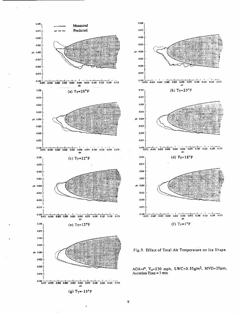
Figure 9 shows ice shape comparison as afunction of temperature at the airspeed of 230 mph.Comparisons show similar results as the lower speedcases. Good agreement is shown at all temperatures
except at 28°F where an overprediction of upperhorn is seen.
Comparison between Calculated and Measured Drag
Calculated drag coefficients were compared withmeasured drag coefficients for the ice shapes shownin Figs.8 and 9. With each icing run, the wakesurvey was made twice: one made while the probetraversed away from the shield, and the other madewhile the plebe traversed back to the shield. Eachmeasured drag coefficient in Table 2 is the averagedvalue of the two measurements at each icing run.Calculated drag coefficients are also included inTable 2 for comparisons.
Results in Table 2 are plotted in Figs. 10 and 11.For both airspeeds, the experimental data showalmost constant measured drag coefficients up toaround 12°F and a sharp increase toward nearfreezing temperatures as the ice shape changes to
glaze ice. For V.= I50 mph, calculated dragcoefficients agree very well with measured drag
coefficients up to 12°F and begin to rise sharply ataround 18°F. While calculated drag coefficients
reach a peak at around 22°F and begin to decrease,measured drag coefficients continue to rise and reach
a peak at around 28°F. For V.,=230 mph, however,the calculated results does a good job of followingthe trend in measured values.
Em_e]uding Remarks
The ice shape and drag coefficient results of theexperimental program conducted in the IRT werecompared with the )redictions using the 2DLEWICE/IBL code. Experimental data providedvalidation data to further calibrate the code withvarious icing parameters such as the temperature,airspeed, and LWC. Good agreement in the ice shapewas shown for the rime ice. The agreementdeteriorated for the glaze ice, although the directionof the horn growth was generally predicted well.Deterioration in ice shape prediction for glaze ice isa typical characteristic shown with the originalLEWICE code. The ice shape comparison resultsindicate that the modifications made to the originalLEWICE code in the process of combining it withthe interactive boundary layer method work well.
The results of the drag comparison study showthe ability of the code to predict the sharp dragincrease displayed by the experimental data as the iceshape changes from rime to glaze. The adjustmentmade by extending the roughness beyond the icinglimit on the airfoil allows the calculated drag valuesto agree well with experimental data. More studiesare needed to better estimate the extent of icing onthe airfoil surface.
The big strength of the 2D LEWICE/IBL code isthe economy of the computing time. A typicalcomputing time (CPU time only) to complete acalculation of 6 or 7 minutes ice accretion and itsaerodynamic characteristics was less than 50 secondson a CRAY X-MP.
More comparison work is needed to check the 2DLEWICE/IBL code for further improvements. Thetest points of the repeatability test in the IRT werereduced from the original test plan due to the loss oftunnel time. More tests are planned to document theeffects of other icing parameters on the ice shape andresulting drag. It is also planned to obtainexperimental lift data with iced airfoils for codevalidation work.
Reference_
1. Cebeci, T., Chert, H,H., and Alemdaroglu, N.,"Fortified LEWlCE with Viscous Effects,"Journal of Aircrafh Vol. 28, No.9, pp. 564-571,Sept. 1991.
2. Shin, J., Berkowitz, B., Chen, H.H., andCebeci, T., "Prediction of Ice Shapes and TheirEffect on Airfoil Performance," AIAA-91-0264,1991.
3. Olsen, W, Shaw, R., and Newton, J., "IceShapes and the Resulting Drag Increase for aNACA 0012 Airfoil," NASA TM 83556, 1984.
4. Soeder, R.H. and Andracchio, C.R., "NASALewis Icing Research Tunnel User Manual,"NASA TM 102319, 1990.
5. Shin, J. and Bond, T, "Results of an Icing Teston a NACA 0012 Airfoil in the NASA LewisIcing Research Tunnel," AIAA-92-0647, 1992.
6. Ruff, G.A. and Berkowitz, B.M., "Users Manualfor the NASA Lewis lee Accretion PredictionCode (LEWICE)," NASA CR 185129, 1990.
7. Cebeci, T., "Calculation of Flow Over IcedAirfoils," AIAA JQl,trnal, Vol. 27, No.7, pp.853-861, 1989.
8. Abbott, I.H. and Von Doenhoff, A.E., Theory ofWing Sections, pp. 462-463, Dover Publications,Inc., 1959.
9. Blaha, B.J. and Evanich, P.L., "Pneumatic Bootfor Helicopter Rotor Deicing," NASA CP-2170,1980.
10.Gregory, N. and O'Reilly, C.L., "Low-SpeedAerodynamic Characteristics of NACA 0012Airfoil Section, Including the Effects of Upper-Surface Roughness Simulating Hoar Frost," NPLAERO Report 1308, 1970.
4

CORNER
C
VARICHRONDRIVE
CONTROL ROC'M
CORNER
B
CORNER
AMC_ELsACCESS DOOR
Fig.1. Plan View of IRT, Shop, and Control Room.
ORtGINAL PAGE
BLACK AND WHITE PHOTOGRAPIt
AOA(deg.)
Table I. Test Conditions
AirSpeed LWC MVD(mph) (ghn 3) (_m)
150 1.O 20
150 1,0 20
150 1.0 20
150 1.0 20
150 1.0 20
150 1.0 20
150 1.0 20
230 0.55 20
230 0.55 20
230 0.55 20
230 0.55 20
230 0.55 20
230 0.55 20
230 0.55 20
TotalTemperature
28
AccretionTime(rain.)
6
25 6
22 6
18 6
12 6
1 6
-15 6
28 7
25 7
22 7
18 7
12 7
1 I_ 7
-15 7
II
Fig.2. NACA 0012 Airfoil and Wake Survey Probe.

0.03
-" 0.020
8L)
g0.01
0.00
t
xi
O
xl
X
4 6 8 I0 12
Angle of Attack, degree
14
Legend: Facility, Reynolds Number
o IRT, 3 Million
• LTPT, 3 Million (Reference 8)
x IRT, 3 Million (Reference 3)
* IRT, 3 Million (Reference 9)
16
0.5
0.4
o 0.3(.,) - .
b/)
o
8 0.2
0.1
0.0
0 2 4 6 8 10
Angle of Attack, degree
Fig. 4. Transition Locations on the NACA 0012 Airfoilfor Re = 2.88 = 106.
Fig. 3. Comparison of Measured Clean Airfoil Drag withPublished Data for the NACA 0012 Airfoil.
Difference fromAverage Ca
Ca = 0.03360 +2.66 %
..... Ca = 0.03308 +1.07 %
CA-- 0.03152 -3.70 %0,100
Average Ca = 0.03273% variation = 3.31% 0.or5
:_I:i_'._!i_,_ nmolii;il,
i 0.02.5
=_llllil_!!iliiiilllii_liliiiiiii__, ........_IiilIilII!Iliili£i!i_!II!i!!I!'' _z=o.ooo
_IIllil!llli £I!Ii!iiiii!Ii!iili_ iiiiil ii! i {i'
0.100
0.075
0.050
0.025
-0.050
-0M75
_.I(X) ___t._l___..L.___ tz__ |.__t__J-_-I z -t .L4t.075 -0.050 ,4),02,,_ 0,_ 0,{17.J O.0.$ll o.lf/5 ILl(X) IL125 1i.1511 11.175
x/e
Difference fromAverage Ca
Ca = 0.03107 -1.77 %
Cd = 0.03293 +4.11%
Ca = 0.03088 -2.37 %
Average Ca = 0.03163% variation = 3.58 %
• :' !•'": ll!_l!!!!lil-"!-=]illiil_i_=!_:],-_i_:_::'*" ;L""7"" i 7
-0.075
-(I.II1_1 ._1 _t__l ,._J._ 1_1...._ __L a_ .I. J. I..., -..-(L(fl5 ..0,11_) 4),(_ 0.1_10 0.1125 0.050 11.1175 (),l(ll) IJ,|'2L5 11.t_41 11175
X/¢
(a) AOA--4 _, V,=150 mph, TT=22°F, LWC=l.0g/m 3,
MVD=20pm, Accretion Time = 6 min.
(b) AOA=4 °, V_=230 mph, TT=22°F, LWC=0.55g/m 3,
MVD= 20t.tm, Accretion Time = 7 rain.
Fig.5, Repeatability of ice Shape and Drag for Glaze Ice Shapes.

0.I00
0.075
0.050
0,02.5
y/_ o.ooo
..O.GZ5
-0,050
_.075
*i ]t]il!l_i_!l!iitii!_lifli_itt_ili_iliiiiiqiiii
......_!i_!iillilii_]ti!!Iiil!!lili_tl
Difference fromAverage Cd
Ca = 0.02313 -0.52 %
Ca = 0.02329 +0.17%
Ca = 0.02334 +0.39 %
Average Ca = 0.02325% variation = 0.47 %
'i[i! i%lTlli_iff_iii[! i !!H!_ii i,
t!iil i_i tt ii_Iiti_!il_Illl fill
i!iiH iii!l!tiiii_!iiii:'
i!t!!l_Ili }iiiiili:ilii!:_l_
iil}!ittliititt_l"
1!I[Itt
ii_illi_i!i iiiiiili'ilii!i_iiili!lit!
-O.I(X) , [ , i , i , l . i , i , 1 , 1 x .J__l__•0.0"/5 -0.050 -0.0_ 0.0100 0.025 0.050 0.075 0.100 0,125 0.150 0.175
(a) AOA=4 °, V.=150 mph, TT=-15°F, LWC=I.0g/m 3,
MVD=201a.m, Accretion Time = 6 min.
Difference fromAverage Ca
0.100
0.075
0.054_
0.025
y/¢ 0.000
-0.1725
-0.050
-0.075
_.|Oll
Ca = 0.02179 +0.65 %
Ca = 0.02149 -0.74 %
Ca = 0.02167 +0.09 %
Average Ca = 0.02165% variation = 0.70 %
!i!iii!!iIi!_:_iiiiTi;iitil_;¸,' ......:_iiiiiiiiiiiii_!ili_i!iil;!iiii!
; _i t l_iil hi_iiill l!ii tii][ _J
_i!ilil]_lI_!lI!l!il!i!li!i!i!l_l fH iiiii i ti i l
_iittt!:!t:-!t!;'ili!f!!!!I!!!I!!!!!',l:if!iiIitiIIiii!1_
!!l!!i!!lilil!iii!!!]!if i
iitill!ii_iii/iiiltil!ll_iiiiii
!ii}iiiiil_l
-0.075 -0.050 -0,_ 0.000 0.025 0.050 0.075 0.100 0.125 0.1511 11.175
I/C
!L
i
(b) AOA--4 °, V.=230 mph, TT=-15°F, LWC=0.55g/m 3,
MVD=201am, Accretion Time = 7 rain.
Fig.6. Repeatability of Ice Shape and Drag forRime Ice Shapes.
Time Increment
6 min.
..... 3 rain.
0.too ---- 1 rain.
o.o7_ .... 0.5 min.
0.050 ..... _: _;: _ :_i_; ii;i iii i iiii!ii;i ii iil i':!i iii i! i i: ill ii ili _ii _i _}_
....__ii }iii ii i_i i]_i I :._ii ii:l: ili i ;_}::::I liii_ll: ii :li_I iiii i_li_i!i!i_iiiii !iii_
0.07.5 iiiiii _iiiiii i i iii i iii il liii iiiHli! 1]i i;i!i I_i :. i;;I]Iii_ !li_ _i!! !i! i ii} _i!l:.i i:.i ::iii ii_i_
-0,025
-0,050 ]
-0075 [
-0.025 0.000 0.025 0.050 0.075 0.100 0.125 0.150 0.175 0.200 0.25
_e
(a) AOA--4 °, V,=150 mph, TT=28°F, LWC=I.0g/m 3,
MVD=201.tm, Accretion Time = 6 rain.
0. IO0
0.075
0.050
0.025
x_ 0.ooo
-0,025
-0.050
......._,_ii _;iitii iliiii!iil i!ii_i Iil iiii i_I i___!_il l i_!;!il!i ii!I!; i!t t!i i_iii#_i,_!
....._r,,_1]!i_i !]!!i,._!I;Hi,_ili;:]!!i i!,.!_!!!ib][]fi_iiil i )! __ :;
-0._5
-0.100 _ I , I , I , I , t L i , i , i , I ,
-0.07 -0.050 -0.{_5 0%100 0.07.$ 0.050 0.075 0.100 0.125 0.150 0.175
X/C
(b) AOA=4 °, V.=150 mph, TT=18°F, LWC=I.0g/m 3,
MVD=201.tm, Accretion Time = 6 rain.
0300
0.075
0.050
0.07.5
_,;c o.ooo
-0.(25
-0.050
-0.075
-0.100-0.07
......_i_;i[_`iiiii_!]1iii]}i_!_!_i_5_!!_!!i[_i_!_]]}!_!Fi_!i!_!!!1_!i!;!!]_i_
_ii i iti HiI[iili!!ii I Ii IIlITIiL_I! I_!_,iii [iiiiih![i!![!!!!_!i!!!i!!!l![i!il _!![_i!ii!Hii!L!!!!
_i1_[_i_i_i_i!i_!_iiiiiii!i_iii_ii_i!_ii_i_i_i_!!_!i_ii_! _]
_1_!;i_!_!_i_!_i_i_i_!_i_ii_iiiiiii_iii!i_!i_iiii!i_i!i_!!_i!iiiii_i_A_i_i!;
:_#T_)_i_;;i_i_}_ii1_i_i]_ii_i:_i_i_i_i_iiii_;i_iii[_i!iii_:`
I I , I _ L • I , i , i , _ _ t • i ,
•0,050 -0._ 0.0_ 0.02_ 0.050 0.075 0. It30 0.125 0.150 0.175
X/C
(c) AOA=4 °, V_=150 mph, TT=-15°F, LWC=I.0g/m 3,
MVD=20gm, Accretion Time = 6 min.
Fig.7. Effect of Computational Time Stepon Ice Shape.

0.100
0.075
0.050
0.02_
.0,1_.5
.0.0._0
4),075
• | • l , I , I" , I , I , I , I , I •
.0.1._.07St'_ .0.050 _ O+O00 O.._.q 0.050 0.075 0.100 O+12.q O+L_I 0.175
0.100
0+075
O.O5O
0_2$
p/_ 0.000
.0_
*0.0YJ
.0.07_
•0.100.0+II
OAIO
0*075
0.0._
0.025
),+_ O*0t_,
0.02_
-0.050
-0*075
. I . I • I • I , I . I , I . I • [
-0,050 ..0.0_ 0._0 0.0_ 0*050 0*075 0.100 0.125 0.150 0.L75x_
(c) TT=22°F
....lli++liil
....+++ ++I+++ii+_i+,_ • =mm_m_++M
_t+ ...... +.+.+.m:i't" : im _l#+. +t+" +if'+_++I+i'+i+ +_+
," k _+!iI +"++' +++j,:,+i +++++++ ....... +'++++++ " J+
"'-.. ++Iiii!P!,_r![ii_l li! lii[li[ I ,+:i[i_i !lli[i!+[ii!]:?i _ [!ibli'_ {ili]!ii!!"
_ i+I!lilli+[t_l!liT_i!i "N(++•,!![
•0.100 , I , I , I , t , _ I _ .J , I , 1 ,++075 +,050 -O._J 0.000 0.0_ 0.050 0,075 0.100 0.125 0,1.._0 0.175
= (_:)TT= 12oF
0.075
0*050
0+O25
p/c O,mO
-0.025
.0.050
-0.ff75
.0.110 , l , I , I , i , l . + . i , I i I +.0.075 .0.0_1 _ O.C_I O.IQS O*0.qO 0.0"/$ 0.100 O.12S 0.150 0.175
Xfc
(g) TT:" 15°F
4).ff75
-.0.|00 , I : I ' ..J.l. | l | . £ , _ l • l •
-0.075 -0.050 .0.07-q 0*000 O,(Y'_ 0.050 0.0'75 O.lO0 0.125 0.150 0.175
x/c
O.IO0
0.075
0.0._
0*025
_/c o.coo
.0*025
+.050
-0.075
(b) TT=25°F
-0. [_0 * I , I * I , I , l + | r l I | I LL
4).075 -0.050 -0.0_ 0*000 0._ 0.050 0.075 0.100 0.125 0.150 0+175
_C
(d) TT= 18°F0300
0.075 +
0.0_
0*025
O.(XX+
+
i
',+,
-0*050 -0,_ 0*000 0.(Y25 0.050 0*075 O.lO0 0.l.?.5 0.1.50 0.175x/e
(f) TT= I°F
-0+O25
..0,_0
-0.075
-0.101]-0+07
Fig.8. Effect of Total Air Temperature on Ice Shape.
AOA--4 °, V.=150 mph, LWC=l.0g/m 3, MVD=201am,Accretion Time = 6 min.
0A00
0.075
0.050
0.025
y/c 0.000
_.026
-0.050
-0.075
Measured
-- -- -- Predicted
[i°-%%. _i
". : ,Mii!li! i r
-0.100 • t * I • I , t • I i t _ I i I _ I L
-0.075 -0.050 -0.0_ 0.000 OJO_ 0.050 O.(T/$ 0.100 0,17.5 0.150 0,175
1/¢
(a) TT=28°F0.I00
0.075
0.050
0.025
_t_ 0.000
-.0.0'2.6
-01050
-0.075
........_i_i))_iiii))ii}iiiiiliiiii_}!li_!)J)i)i)i!i)!}i
/oo
!i_ !_!__iI_
4)'1-0.075 -0.0J0 -0.025 0,000 0.025 0.050 0.075 0.100 0.125 0.150 0.175.
0.100
0.075
0.050
0.025
y/¢ 0.000
-0.025
-0.050
-0.075
-0.100-0.07
0.1(30
0.D75
O.I150
0.07_5
:tic o,o_o
-0.ol5
-0.Q5o
-0.075
(c) TT=22°F
," ii_r
•..... "_:_:!_?h!!_i}!!_l_i!il}!}ii!_il_i_i_i_i)}i{i}i_[_i}li_Til}_[]!?j!}ii_}iti[:_!}_!i_? _;¢
•.O.0JO -0.0_ 0.000 0.0_ 0.0.T0 0.075 0.100 0.125 0.150 0.175
(e) TT = 12°F
-0.1{]0 , I , I , I _ I , I , I _ I , ] _l
-0.O75 -0.050 -0.025 0.000 0.025 0.050 0.075 O, lOO 0,125 0.150 0. i75
X/C
(g) TT=- 15°F
0.100
0,075
0,050
0.025
x/_ o.ooo
..0,025'.:_;=[:i!tl!!liqHl_lilii;[!l[:[:;[_}i _ ,_ _ !_H!Hfi H [[! ii_ !{il_}i[liI}ii]}ii } hi}}1 ! [i } }=:!
: !_:':'__i!i}il}_};}[i{}!}i[}i!{f}{{l!}i}!i!{};i{i]}ii}]}[i}i}}i}i}[!l-_.0,._
-0.075
-0,1(30 ,_ f ' _ ' I , I _ I = L__-L,-_Z_'. 1_-0,075 -0.050 -0,02S 0.000 O.ff15 0.0._) 0.075 O.lO0 0,125 0.150 0.175
I/C
o.1oo (b) TT=25°F
0.075
0.051) _i:.,iiiiiiiiiiiiii....._iiiiu_!iiiii!iiiiiiiiiliiii!ii :i'F!'!_'i",'?/_?i'ii"?'i
yl¢ 0.0(X1
i ;iti iliii i_h i!_1!_}i!_iit!ii]ii ill _!!_i.i!ill[i!i :iii_iit[ii!iiii}!}i!ii}iii;!l!ii-0.0"15
[[k}}ii_.{ii;!i}_i:_i}iE
-0,075
-0.075 -0.050 -0.025 O.O00 0.025 0.050 0,075 O.lO0 0.125 0,150 0.175
x,'c
o.,_o (d) TT= 18°F
(1.075
I
0.02J il}[:i:H_ I_qHP'I_::H: ;::! ....... ::_::[i:i}[i{{_
; !qi_!:.!i![i}irl_] ] [ !i!}i}{__[{}}!{i {}!iii![:][]l}i :.[ i] _;:ii[:}[]i}}_}i _I t[]{}Li}{lil i i :[ ii[!{_{}ii[:• ]
", [!-0.ff_
-O.O5O
-0.075
41.075 -0,050 -0.02,5 0.000 0.025 0.050 0,075 O.IDO 0,125 0.154] 0.175
_Jc
(f) TT=I°F
Fig.9. Effect of Total Air Temperature on Ice Shape.
AOA=4 °, V**=230 mph, LWC=0.55g/m3, MVD=20t.tm,Accretion Time = 7 rain.
9

Table 2. Effect of Total Air Temperature on Drag Coefficient.
(a) Airspeed=150 mph, LWC=I.0g/m3, MVD=201am
Total Experimental CalculatedTemperatttre Drag Drag
(OF) Coefficient Coefficient
28 0.0578 0.0346
25 0.0540 0.0372
22 0.0315 0.0392
18 0.0271 0.0351
12 0.0229 0.0217
1 0.0229 0.0209
-15 0.0233 0.0202
(b) Airspeed=230 mph, LWC=0.55g/m3, MVD=201am
Total Experimental CalculatedTemperature Drag Drag
(OF) Coefficient Coefficient
28 0.0428 0.0470
25 0.0371 0.0294
22 0.0311 0.0202
18 0.0268 0.0195
12 0.0255 0.0195
1 0.0234 0.0195
-15 0.0218 0.0192
r,Y
4.)
0.08
0.07
0.06
0.05
0.04
0.03 ---
a0.02 --o
0.01
0.00 _
°20
a .Experiment• Calculation
D
m
-10 0
g
w
10 20 30 40
Total Temperature, OF
Fig. 10. Effect of Total Temperature on Drag ( V. = 150 mph).
0.08
0.07
0.06
0.05
_ 0.04
0.03
r_
..._.._J J_
t_ Experiment
• Calculation
0.02 o _)
0.01 ........
0.00 , .
-20
o-"
D D_
'"O ...... 1)" *o ..............................
-10 0 10 20 30 40
Total Temperature, OF
Fig. 11. Effect of Total Temperature on Drag ( V,,=230 mph).
10


I Form ApprovedREPORT DOCUMENTATION PAGE OMB No. 0704-0188
Public reporting burden for this collection of information iS estimated to average 1 hour per response, including the time for reviewing instructions, searching existing data sources,
gathering and maintaining the data needed, and completing and revlewieg the collection of information. Send comments regarding this burden estimate or any other aspect of this
collection of information, including suggestions for reducing this burden, to Washington Headquarters Services. Directorate for information Operations and Reports, 1215 Jefferson
Davis Highway, Suite 1204. Arlington. VA 22202-4302, and to the Office of Management and Budget, Paperwork Reduction Project (0704-0188). Washington, DC 20503.
1. AGENCY USE ONLY (Leave blank) 2. REPORT DATE 3. REPORT TYPE AND DATES COVERED
January 1992 Technical Memorandum
4. TITLE AND SUBTITLE 5. FUNDING NUMBERS
Experimental and Computational Ice Shapes and Resulting Drag Increase
for a NACA 0012 Airfoil
s. AUTHOR(S)
Jaiwon Shin and Thomas H. Bond
7. PERFORMING ORGANIZATION NAME(S) AND ADDRESSOES)
National Aeronautics and Space Administration
Lewis Research Center
Cleveland, Ohio 44135-319]
9. SPONSORING/MONITORING AGENCY NAMES(S) AND ADDRESS(ES)
National Aeronautics and Space Administration
Washington, D.C. 20546-0001
WU-505-68-10
8. PERFORMING ORGANIZATIONREPORT NUMBER
E-7148
10. SPONSORING/MONITORINGAGENCY REPORTNUMBER
NASA TM- 105743
11. SUPPLEMENTARY NOTES
Prepared for the 5th Symposium on Numerical and Physical Aspects of Aerodynamic Flows, sponsored by California
State University, Long Beach, California, 90810. Jaiwon Shin and Thomas H. Bond, NASA Lewis Research Center.
Responsible person, Jaiwon Shin, (216) 433-8714.
12a. DISTRIBUTION/AVAILABILITY STATEMENT
Unclassified - Unlimited
Subject Category 02
12b. DISTRIBUTION CODE
13. ABSTRACT (Maximum 200 words)
Tests were conducted in the Icing Research Tunnel (IRT) at the NASA Lewis Research Center to document the
repeatability of the ice shape over the range of temperatures varying from -15 °F to 28 "F. Measurements of drag
increase due to the ice accretion were also made. The ice shape and drag coefficient data, with varying total tempera-
tures at two different airspeeds, were compared with the computational predictions. The calculations were made with
the 2D LEWlCE/IBL code which is a combined code of LEWICE and the interactive boundary layer method devel-
oped for iced airfoils. Comparisons show good agreement with the experimental data in ice shapes. The calculations
show the ability of the code to predict drag increases as the ice shape changes from a rime shape to a glaze shape.
14. SUBJECT TERMS
Ice Accretion; Aerodynamic characteristics; Roughness
17. SECURITY CLASSIFICATIONOF REPORT
Unclassified
NSN 7540-01-280-5500
18. SECURITY CLASSIFICATIONOF THIS PAGE
Unclassified
19. SECURITYCLASSIFICATIONOF ABSTRACT
Unclassified
15. NUMBER OF PAGES12
16. PRICE CODE
A03
i 20. LIMITATION OF ABSTRACT
Standard Form 298 (Rev. 2-89)
Prescribed by ANSI Std. Z39-18
298-102