ARTIFICIAL INTELLIGENCE 49

Shape from Regular Patterns

Katsushi Ikeuchi Electrotechriical Laboratory, Utnezono- 1- 1-4, Sakura-tn ura, Niihari-gun, Ibaraki, 305, Japati

Recommcndcd by Michael Rrady

ABSTRACT

niis paper describes an aigoritlitr1 to obtaitl local surface orierltatiorr frofti the apparetlt surface-pattertl distortion in an image.

We propose a spherical projection to model perspctiue imaging. A trtappitlg is debtled based of1 the measurement of the local distortions of a repeated known rexture pattern due Io the image projection. 77tis mapping maps an apparent shape on the image sphere lo a locus of possible surface orienrations on the Gaussian sphere.

A n ireratiw constraint propagation algorithm with the orientations at occluding boundaries reduces possible surface orientations to a unique orientation. 7 l i s algorithm can recover local surface orientation as well as interpolate surjace orientations where no information is auailable. ?Xis algorithm is applied to a real image ro demonstrate its perfontlance.

0. Introduction

Information about surface within boundaries comes from various sources such as stereopsis, shading, high-light and texture gradient. This information is converted into local surface orientation, often referred to as a 2-1/2 D sketch [2,3], or a needle map 141. This paper concentrates on making this 2-1/2 D sketch from texture gradient .

This domain, referred to as the shape-from-texture problem, has been studied extensively [5-121. Historically, Gibson pointed out the role of texture as a basis for the recovery of surface orientation [5 ] . He proposed the density gradient as the primary basis for surface perception by humans.

Formalizing the shape-from-texture problem requires modeling the image- forming system. Mainly two kinds of projections have been commonly used: the orthographic projection and the perspective projection. Kender [7], Kanade [SI, and Witkin [ 101 explorzd the domain under the orthographic projection. Kender formalizes the relationship between local surface orien- tation and two perpendicular texture elements assumed to have the same

Artificial Intelligence 22 (1984) 49-75 0004.3702/84/$3.00 @ 1984. Elsevier Science Publishers B.V. (North-Holland)

50 K. IKEUCHI

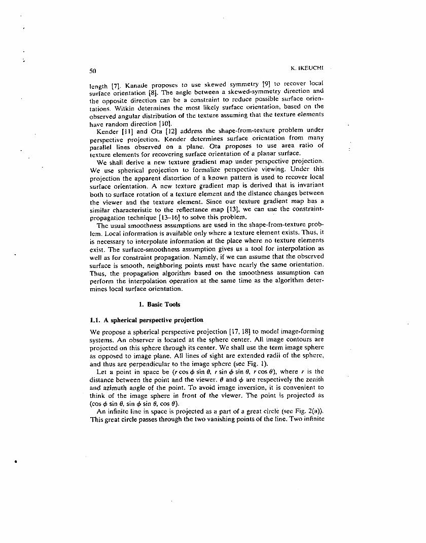
length [7]. Kanade proposes to use skewed symmetry 191 to recover local surface orientation [8]. The angle between a skewed-symmetry direction and the opposite direction can be a constraint to reduce possible surface orien- tations. Witkin determines the most likely surface orientation, based on the observed angular distribution of the texture assuming that the texture elements have random direction [lol.

Kender (1 11 and Ota [ 12) address the shape-from-texture problem under perspective projection. Kender determines surface orientation from many parallel lines observed on a plane. Ota proposes to use area ratio of texture elements for recovering surface orientation of a planar surface.

We shall derive a new texture gradient map under perspective projection. We use spherical projection to formalize perspective viewing. Under this projection the apparent distortion of a known pattern is used to recover local surface orientation. A new texture gradient map is derived that is invariant both to surface rotation of a texture element and the distance changes between the viewer and the texture element. Since our texture gradient map has a similar characteristic to the reflectance map [13], we can use the constraint- propagation technique [ 13-16) to solve this problem.

The usual smoothness assumptions are used in the shape-from-texture prob- lem. Local information is available only where a texture element exists. Thus, it is necessary to interpolate information at the place where no texture elements exist. The surface-smoothness assumption gives us a tool for interpolation as well as for constraint propagation. Namely, if we can assume that the observed surface is smooth, neighboring points must have nearly the same orientation. Thus, the propagation algorithm based on the smoothness assumption can perform the interpolation operation at the same time as the algorithm deter- mines local surface orientation.

1. Basic Tools

1.1. A spherical perspective projection

We propose a spherical perspective projection [17, 181 to model image-forming systems. An observer is located at the sphere center. All image contours are projected on this sphere through its center. We shall use the term image sphere as opposed to image plane. All lines of sight are extended radii of the sphere, and thus are perpendicular to the image sphere (see Fig. 1).

Let a point in space be (r cos 4 sin 8, r sin (b sin 8, r cos e), where r is the distance between the point and the viewer. 8 and (b are respectively the zenith and azimuth angle of the point. To avoid image inversion, it is convenient to think of the image sphere in front of the viewer. The point is projected as (cos qJ sin 8, sin qJ sin 8, cos 8).

An infinite line in space is projected as a part of a great circle (see Fig. 2(a)). This great circle passes through the two vanishing points of the line. Two infinite

SHAPE FROM REGULAR P A T E R N S 51

(r cos+ sin6.r s i n

/ ,e AN IMAGE SPHERE

0 /

’

\ / ‘\ ’

4 s i n 8 . r cos 8 )

FIG. 1. An image sphere. All contours are projected on the image sphere through t h e center.

parallel lines in space are projected as two great circles. These great circles intersect each other at the vanishing points. An infinite plane is projected as a hemisphere. A line on the plane has vanishing points on the boundary of the hemisphere. The normal direction on the plane corresponds to the center of the hemisphere (see Fig. 2(b)).

1.2. Comparison with other image projections

Two image-forming models have been commonly used; the orthographic and perspective projections. This paper refers to the conventional perspective projection as plane perspective projection.

1.2.1. Orfhographic projection

If the size of the objccts is small compared to the viewing distance, then the image-forming system can be approximated as an orthographic projection. To standardize the image geometry, the viewer direction is aligned with the z-axis. The object point (x, y , z ) maps into image point (u, u ) where u = x and u = y (see Fig. 3(a)).

1.2.2. Plane perspective projection

Fig. 3(b) illustrates a plane perspective projection. The object point (x, y , z) maps into image point (u, u ) where u = (x / - z ) and u = (y/-z).

Both the orthographic projection and the spherical perspective projection have lines of sight perpendicular to the image plane (sphere). Thus, neither thc

52 K. IKEUCHI

FIG. 2. Characteristics of thc sphcrical pcrspcctivc projcction.

orthographic projection nor the spherical perspective projection have any image distortion due to a pattern's position on the image plane. On the other hand, under the plane perspective projection, the angle between the line of sight and the image plane depends on the location of the image point. Thus, the shape of the projected pattern will generally vary with its location, even though the line of sight maintains the same angle with the pattern's surface normal.

Both the spherical perspective projection and the plane perspective pro- jection have only one viewing position. The two perspective projections exhibit the distance effect: a far object projects a smaller image than a near object.

SHAPE FROM REGULAR PAmERNS

A Y

P

53

(U. v. -1)

z -

FIG. 3(a). The orthographic projection.

V

U

(X. Y. 2 )

(X. Y. Z)

Y

X

X z u e--

FIG. 30) . The plane perspective projection.

Y v = - - z

The orthographic projection, with infinite focal length, does not exhibit the distance effect.

The spherical perspective projection has several advantages over the plane perspective projection.

(1) We can use a uniform-texture gradient map at every point on the image sphere.

K. IKEUCHI 54

Lines of sight are everywhere perpendicular to the image sphere. Thus, all contours on the image sphere are foreshortened only due to the relationship between the line of sight and the surface normal. On the other hand, the plane perspective projection distorts a pattern twice. The first distortion is due to the angle between the surface normal and the line of sight. The second one occurs due to the angle between the line of sight and the image plane. The second distortion depends on the position of a pattern on the image plane.

(2) We can make smooth mosaic images taken from the same position but in different viewing directions.

The spherically projected pattern of an object does not change when the viewer direction changes provided that the viewer and the object maintain constant position. This is not the case with the plane perspective projection where the image plane is rigidly fixed to the viewing direction. The image-plane direction changes the apparent pattern of an object, even though neither the object position nor the viewer position change. Thus, we cannot make meaningful mosaic images taken in diferent directions under plane perspective projection.

(3) The spherical perspective projection has psychological validity. The most sensitive area of the retina extends to only 3-4 degrees over the

visual field. Eye movements (and head movements) are required to examine patterns in different directions. Thus, the line of sight is always perpendicular to the image plane. Several examples favor the spherical perspective pro- jection.

Example 1.1. Consider an infinite plane surface covered with small squares parallel to the image plane under the plane perspective projection (Fig. 4). The

THE VIEWER

FIG. 4. A defect of perspective projection. The perspective projection does not exhibit fore- shortening for objects on planes parallel to the image plane.

SHAPE FROM REGULAR PATTERNS 55

squares on the plane always project as squares on the image plane, no matter where the squares lie on the surface. While under the spherical perspective projection the squares would appear as various rectangles depending on their positions on the surface, which is more similar to our observation.

Example 1.2. If we were to observe a laser beam projected from the ground to the sky, the lighting locus would be a circle connecting the ground with the zenith. An infinite line in space is projected as a great circle.

Example 1.3. We observe the horizon as a circle. This is because an infinite plane (the ground) is projected as a hemisphere. The horizon is the vanishing l ine of the ground.

Example 1.4. Many kinds of insects have compound eyes that give rise to a projection like that in the image sphere.

The usual man-made image-forming system has a planar sensitive area. This is the reason why the plane perspective projection is often used. However, the image on the image plane can be easily converted into the image on the image sphere. Let a point on the image plane be (u, v ) . Then the point is mapped into

(up/ 1 + u’ + v’, v/v 1 + u’ + v’, l/V 1 + u’ + v’) .

1.3. Gaussian sphere and image sphere

Surface orientation is expressed using the Gaussian sphere [14]. The Gaussian sphere is a sphere of unit radius whose z-axis is taken as an extended line through the north and south poles of the sphere. Assume that we put a surface patch of an object at the center of the sphere and that the direction of the viewer is the direction from the center to the north pole. The surface patch faces some point on the sphere. For example, if a surface normal has the same direction as the north pole, the surface patch is perpendicular to the line of sight. All possible orientations of a surface patch are represented on the Gaussian sphere. Thus, we can describe local surface orientation o n an object in terms of points on the Gaussian sphere.

Note that there are two spheres: the image sphere and the Gaussian sphere. Consider, now, Fig. 5. The image sphere is a viewer-centered spatial coordinate system with which the image is specified. The Guassian sphere is also viewer- centered, and measures surface orientation relative to t h e north-south axis of the sphere, which always points at the viewer. When a pattern is at the south pole of the image sphere, the coordinate system on the Gaussian sphere is the same as the coordinate system of the image sphere. When a pattern exists at some other point on the image sphere, then one must rotate the Gaussian sphere so that its north-south axis aligns with the viewing direction. Appendix

56 K. IKEUCHI

/ i i

GAUSSIAN SPHERES

1 I

THE IMAGE SPHERE

/ / /

/

FIG. 5. The Gaussian sphere and the image sphere. All possible orientations of a surface patch on the image sphere are represented on the Gaussian spheres based on the local direction of the viewer.

B gives a formalized relationship between the Gaussian sphere and the image sphere.

2. Measuring Texture Distortion due to Surface Orientation

2.1. Definition of the problem

We shall determine surface orientation from the apparent distortion of regular patterns on an image sphere, provided that:

(1) The surface is covered with uniformly repeated texture elements. We call the uniform texture a regular pattern.

(2) Each texture element is small, compared with the distance between the viewer and the element. If the texture element is small, the element can be regarded as projected onto a tangential plane of the image sphere.

(3) Each element is small, compared with a change of surface orientation there. Each texture element is assumed to lie in the. plane of the viewed surf ace.

(4) The original shape of the texture element (a generator) is known. Since

SHAPE FROM REGULAR P A n E R N S 57

we shall decode surface orientations from the apparent distortion of a pattern, it is necessary to have a standard pattern with which to compare the distorted pattern. This requirement is similar to that of the albedo ratio in using the reflectance map. If one does not know the albedo ratio, one cannot make a correspondence between actual intensities and brightness values on t he reflectance map.

2.2. A measure for distortion in regular patterns

This section examines the relationship between surface orientation and ap- parent pattern distortion. Fig. 6 shows the spherical projection of squares in various orientations on a plane inclined 45 degrees in the vertical direction. Even though the generators (squares) lie on the same tilted plane, their images are different from each other. Their distortion depends on two factors. One factor is the surface orientation. This is what we arc interested in. The other is the orientation of the squares in the plane of the surface. This 'in-surface' rotation causes the variations shown in Fig. 6. Our goal is to find some intrinsic measurement that depends only on surface orientation.

If two perpendicular axis vectors can be associated with a texture element in a.unique manner [8], we can use this pair of vectors as a kind of generalized texture element (see Fig. 7). When a pattern is distorted because of the angle between the surface normal and the line of sight, the two vectors will also be distorted. This distortion of two axis vectors is the same as t h e distortion of the

. . . . . . .1-1. . . . I : : :o:I ; A ;b. . . . . , .

'0:. . . . . . . . . . . : : : : : : . :o . . . . . ' 8 ' " '

. . . . . . . . . . - . . . . . . . . . . . . . . . . . . . . . . . . . . . . . . . . . . . . .

. . . . . . . . . . . . . . . . . . . . . . . . . . . . 'El 1-1.

. . . . . . . . . . . . . . . . . . . . . . . . . . . . . . . . .o :eo: . . . : : . . . . . . .

. . .

FIG. 6. Projection of squares. All squares lie on a plane inclined in north-south 45 degrees and east-west 0 degrees. Their distortion depends on both the orientation of the surface and the orientation of the squarcs in the planc of the surface.

K. IKEUCHI 58

regular pattern, because the axis vectors are fixed on the regular pattern. We shall, therefore, concentrate on distortion of two axis vectors.

The calculation in Appendix A shows us that the magnitude of the cross-product of two axis-vector projections is proportional to cos w and the sum of squares of their lengths is proportional to 1 + coszw where w is the angle between the direction of the viewer and the direction of the surface orien- tation. These two values depend only on the surface orientation; and they are independent of the 'in-surface' rotation angle of the regular pattern. For example, the patterns in Fig. 6 will yield the same value since they exist on the same tilted surface.

The ratio of two axis-vectors' cross-product to their squared length sum is the desired measure for the regular pattern gradient map. The length of a small object on the image sphere depends on the distance between the viewer and the object. A distant object is small while a near object is large. Both the cross-product and the sum of squares of length depend on the distance, but these effects cancel when their ratio is taken, as shown in Appendix A. Thus, the ratio is independent of the distance between the viewer and the pattern. This ratio is also independent of the viewer's orientation, because of the spherical perspective projection. The ratio only depends on the angle between the line of sight and the surface normal. This means that we can use the same regular pattern gradient map everywhere on the image sphere.

We shall call I in (1) the distortion value.

I = f g sin T/V + g')

. . . . .

. . . . . :::::I

. . . . . . . . . . . . . . . . . . . . . --m-- J-.; . . . . . . . . . . . . . . . . . . . . . . . . . . . . . I .

. ' ' . Q..

)(I I+:": . . . . . . : : ': . . . . . . . . . . . . . . .

FIG. 7. Pairs of axis vectors.

59 SHAPE FROM REGULAR PAITERNS

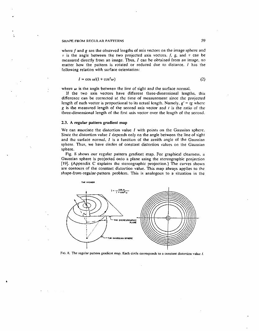
where f and g are the observed lengths of axis vectors on the image sphere and T is the angle between the two projected axis vectors. f, g, and T can be measured directly from an image. Thus, I can be obtained from an image, no matter how the pattern is rotated or reduced due to distance. I has the following relation with surface orientation:

I = cos W/(l + COS’W)

where w is the angle between the line of sight and the surface normal. If the two axis vectors have different three-dimensional lengths, this

difference can be corrected at the time of measurement since the projected length of each vector is proportional to its actual length. Namely, g‘ = rg where g is the measured length of the second axis vector and t is the ratio of the three-dimensional length of thc first axis vector over the length of the second.

2.3. A regular pattern gradient map

We can associate the distortion value I with points o n the Gaussian sphere. Since the distortion value I depends only o n the angle between the line of sight and the surface normal, I is a function of the zenith angle of the Gaussian sphere. Thus, we have circles of constant distortion values on the Gaussian sphere.

Fig. 8 shows our regular pattern gradient map. For graphical clearness, a Gaussian sphere is projected onto a plane using the stereographic projection [ 191. (Appendix C explains the stereographic projection.) The curves shown are contours of the constant distortion value. This map always applies to the shape-from-regular-pattern problem. This is analogous to a situation in the

THE VIEWER

THE STEREUGRAPHIC PLANE

THE GAUSSIAN S?tERE

FIG. 8. The regular pattern gradient map. Each circle corresponds to a constant distortion value I.

60 K. IKEUCHI

shape-from-shading problem where the surface is known to be a Lambertian reflector and the light source is known to be near the viewer.

Fig. 9(a) illustrates how to use the map on the Gaussian sphere and the image sphere. The locus of possible surface orientations for a particular distortion value is a circle o n the Gaussian sphere. The circle center cor- responds to the direction of the line of sight. The radius of the circle is obtained from the distortion valuc I.

Fig. 9(b) shows three square pieces of paper imaged from three vantage points. Distortion values 11, 12, I , were calculated using (1).

The stereographic projection preserves circles (a circle on the image sphere projects to a circle on the stereographic plane). Thus, we can work with circles on the stereographic plane instead of circles on the image sphere. Their centers are the projected viewing directions, and their radii can be calculated from the distortion values I and the projected viewer directions (f, g) (see Fig. 9(c)).

Threc circlcs intcrscct cach othcr at a point which gives the surface orien- tation.

J FIG. 9(a). The regular pattern gradient map and the image sphere: spatial configuration. The circle denotes possible surface orientations. The center of the circle is the direction of line of sight in the image sphcre (a spatial coordinate systcm). Thc radius of thc circle is obtained from the distortion vnluc.

SHAPE FROM REGULAR PATTERNS

FIG. 9@). The regular pattern gradient map and the image sphere: observed apparent shapes.

61

. __ . .

62 K. IKEUCHI

FIG. 9(c). The regular pattern gradient map and the image sphere: loci on the stereographic plane. Each locus on the Gaussian sphere is projected on the same stereographic plane. Since the stereographic projection is a circle-preserving mapping [19]. we also obtain a circle on the stereographic plane. The center position and radius of each circle can be obtained using the definition of the stereographic projection in Appendix C.

3. Constraints and the Propagation of Constraints

3.1. The smoothness constraints

Surface smoothness requires that the surface orientation be continuous over the image sphere. Our smoothness requirement is equivalent to the require- ment that the surface height function be c' on the image sphere [14):

(1) Surface is continuous on an image sphere (co w.r.t. height). (2) Surface orientation is continuous on an image sphere (c' w.r.t. height). The definition of continuity can be expressed in a more convenient form: A function F, is continuous at (xo, yo) if, given E > 0, there exists a S such that

when (x - x0)' + 0, - yo)2 < 8, then '

If, given a particular E, we can find a single value of 6 for all points in the region of interest, then the function is uniformly continuous.

We shall tessellate an image sphere into a discrete grid. If we take the grid

SHAPE FROM REGULAR PATTERNS 63

interval So smaller than 6, then we can guarantee that:

IFXxo+ 60, yo) - E(xo, yo)\ -= E and ~F, (XO, yo+ SO) - E(xo, YO)^ < E .

(3)

Note that surface orientation is assumed to vary continuously o n the image sphere. A more extended discussion can be found in [9].

3.2. Regular pattern gradient map and a propagation algorithm

The smoothness constraint can be used to reduce the locus of possible orientations on the Gaussian sphere. Each distortion value corresponds to a circle on the regular pattern gradient map. A propagation algorithm from the smoothness constraints reduces this locus of possible surface orientations to a unique orientation.

We can measure the departure from 'smoothness' as follows:

The error in the regular pattern gradient map can be stated this way:

( 5 ) p. = [ I . . - R(F.. G..)]' 11 11 'I' v

where F and G denote surface orientations. Iij is a distortion value measured at ( i , j ) . R is the regular pattern gradient map. A solution should minimize the sum of the error terms over all nodes:

e = c (si, + Arii) . i j

The factor A weights the errors in the regular pattern gradient map relative to the departures from surface smoothness.

We differentiate e with respect to F and G, obtaining exactly as in [14],

,

64 K. IKEUCHI

3.3. Occluding boundary constraints (external constraints)

The surface normal is uniquely determined at smooth occluding boundaries [14, 20, 211, being orthogonal to the line of sight and to the contour (see Fig.

The shape-from-shading work in [14] used the orthographic projection, while we use the spherical projection here. However, since the image sphere is perpendicular to all lines of sight in the spherical projection, the occluding- boundary result holds.

This occluding information gives us strong boundary conditions. The pro- pagation constraints only convey information. In other words, constraint pro- pagation determines a relative relationship between nodes but cannot create new information. The surface orientation is fixed at occluding boundaries. From these boundaries' we can propagate the information inward over the image points, adjusting the propagated value with the local constraints provided by the distortion value at each point.

10).

4. Experiments

4.1. Experiment 1: a synthesized image

Consider a plane covered by many squares. The squares are projected onto an image sphere using the spherical perspective projection. Fig. 11 shows the synthesized image in stereographic projection. Note that the infinite horizon line maps to a circle. For the purposes of this experiment, we take this circle to be equivalent to an occluding boundary and assume the surface orientation o n the circle is fixed (Fig. 2(b)).

THE VIEWER

LINES OF SIGHT

SILHOUETTE

FIG. 10. Occluding boundary constraints. At an occluding boundary the surface normal is uniquely determined. This occluding information gives us the boundary conditions.

. SHAPE FROM REGULAR PATTERNS 65

FIG. 1 1 . A synthesized image (in stcrcographic projcction). A planc covcrcd by many squares is projected onto an image sphere.

The process has three main stages. The first stage examines the image to obtain distortion values and surface orientations on the occluding boundaries. The second stage is the main one. This stage computes surface orientation for all points using the propagation method. Since the surface orientations obtained at the second stage are expressed in a viewer-centered coordinate system, the third stage converts the result to the representation in the spatial coordinate system.

We get the distortion using (I ) . The silhouette on the image sphere deter- mines orientation at the occluding boundaries. The distortion values and surface orientations are input for the propagation algorithm. Fig. 13 shows the distortion valucs and Fig. 14 shows surface oricntations at the occluding boundary.

The propagation algorithm estimates surface orientation at each point and is applied iteratively at each point, using the values of surrounding points and the corresponding distortion value. These estimates are the input information to the next iteration. When the entire system of points reaches a stable state, the algorithm stops.

Fig. 15 shows the needle diagrams obtained for a planar surface after 50 iterations. They are expressed using the viewer-centered coordinate system, where the line of sight is taken as the z-axis at each point. Note that the physical direction is different at each image point because of the spherical perspective projection. Fig. 16 is the planar surface depicted in the viewer- centered coordinate system.

66 K. IKEUCHI

AN IMAGE ii DISTORTION VALUES

(2) - - -

(3) - - -

PROPAGATE CONSTRAINTS --w

SURFACE NORMALS IN THE VIEWER-CENTERED COORDINATE SYSTEM

SURFACE NORMALS IN THE SPATIAL

COORDINATE SYSTEM

FIG. 12. Three stages. ( I ) To obtain distortion values and occluding boundary surface orientations. (2) To compute surface orientation for all points. (3) To convert surface orientation in viewer- centered coordinates into the spatial coordinate system. (If an object is small compared with its distance this stage may be omitted.)

FIG. 13. Distortion values obtained from the synthesized image. I = /g sin d(f2 + g*).

SHAPE FROM REGULAR PA7TERNS 67

. . . . . . . . . . . . . . . .

. . . . . . . . . . . . . < < I . . . . x v \ \ . . . . X i \ . . .i\\. : : : 1 . .\\ . . . . . . . .\\ . . . . . . . . .\\ . . . . . . . . . .\\ . . . . . . . . . . . . . . . .\ . . . . . . . . . . . . . . . . . . . . . . . . .\-- . . . . . . .

t t l t f . . . . . . . . . . . . . . . . . . . . . . . . . . . . . .

.\- . . . . . . - . . . . . . . - . . . . . . . - . . . . . . . - . . . . . . . . . . . . . . - . . . . . . . - . . . . . . . .~~ . . . . . . .~~ ....... . .~ . . . . . . :<<: : : : : . . . .

. .

. .

~ . . . . . . . . . . 1 1 7 7 : : 1 : : : :: . . , / / / . . . . / / z : : : : . . . . . . //. . . . . //. . . . 00. . . . . /0. . . . . . . . . . . . . . . . . . . . . . . . . . . . . . . . . . . . . . . . . . . . . . . . . . . . . . . . . . . . . . . . . . . . . . . . . . . . . . . . . . . . . . . . . . . . . . . . . . . . . . . . . . . . . . . . . . . . . . . . . . . . . . . . . . . . . . . . . . . . . . . . . . . . . . . . . . . . . . . . . . . . . . . . . . . . . . . . . . . . . . . . . . . . . . . . . . . . . . . . . . . . . . . . . . . . .

. . . . . . . . [ I .

... H . . . . .00. . . .00.

..,.e . . . . -

....a . . . . - . . . . - . . . . - . . . . - . . . --. .. . . . . . . ..’ \.. .... . . . . . . . . . . . . . . . . . . . . . . . . . . . . . . ....... t ( I I l ”

. X i . . . . . . . . . . . . . . . . . . \:: . . . \\>:

FIG. 14. Surface orientations from occluding boundaries.

. .

. . . . . . . . .. ..

> A : , ......... FIG. 15. The resulting needle diagram.

FIG. 16. A planar surface depicted in the viewer-centered coordinate system.

68 . K. IKEUCHI

Fig. 17 shows the same surface in the spatial coordinate system. The main source of error comes from the digitization of the third process.

4.2. Experiment 2: a real image (a golf ball)

We shall compute the surface orientation for a golf ball using its surface texture. A golf ball has many small circles on its surface. The distortion of these circles can be used to recover local surface orientations. Fig. 18 shows the input picture.

We can get distortion values from this picture by drawing two parallel lines in an arbitrary orientation tangent to each circle (see Fig. 19). We connect the resulting tangent points on each circle and use the connecting line as one of the axis vectors. We then draw a line parallel to the tangential lines through the center of the first axis vector. The part of this line within the projected circle is the second axis vector. We can compute the distortion values using (1). Fig. 20 shows the distortion values obtained.

We can determine surface orientation by using the algorithm. In this case the object is very small compared with the distance between the viewer and the object. Fig. 21 shows the resulting surface in the spatial coordinate system after 50 iterations.

VIEW ANGLE tan-’ 10.0

FIG. 17. The planar surface in the spatial coordinate system.

SHAPE FROM REGULAR PA'ITERNS 69

FIG. 18. A picture of a golf ball. The distortion of the small circles on the golf ball can be used to recover local surface orientations there.

.

\

FIG. 19. How to get a pair of axis vectors from a circle.

FIG. 20. Derived distortion values. Each needle corresponds to a little circle on the golf ball and expresses how much the little circle is distorted there.

70 K. IKEUCHI

. . . . . \ I f / / . . .<I \ I I / I l l : . . . .

. . . : i V \ t I I I I I / I / .

. . . . . . . . . \ \ \ \ \ I I I I I I / / / / .

FIG. 21. A computed result.

5. Conclusions

REALSURFACE

OBTAINED SURFACE FROM THE ALGORITHM

(1) We proposed a spherical projection to model perspective viewing. (2) We defined a distortion value for a regular pattern and proposed a regular

pattern gradient map using this measure. (3) We showed that the propagation algorithm can successfully determine

surface orientations from regular pattern gradients using the spherical perspec- tive projection, the regular pattern gradient map, and occluding boundary constraints.

Appendix A. Derivation of the Distortion Value Z

Fig. A. l shows the relationship between the viewer and a regular pattern; the viewer is at V = (O,O,cos 0") and the texture element is at R =

SHAPE FROM REGULAR PA'ITERNS

1' 71

NORMAL)

FIG. A. l . Relationship between the viewer and a regular pattern.

(-cos 4" sin e,, -sin 4, sin e,, 0). Thus, the viewer vector V is

V = (cos 4, sin e,, sin 4, sin e,, cos 8,)

The surface normal of a plane on which the regular pattern lies can be denoted as

N = (cos 4 sin 8, sin 4 sin 4, cos 8)

in the spatial coordinate system. We can take the two base vectors of this surface as

X = (sin 4, -cos 4,O) , Y = (cos 4 cos 8, sin 4 sin 8, -sin 8). (A.1)

X is a unit vector which lies on the intersection between the image plane and

72 K. IKEUCHI

the surface on which the regular pattern lies. Thus, a general form for two axis vectors of the regular pattern is A, B:

A = ( X cos a + Y sin a ) , B = ( - X sin a + Y cos a) ( A 3

where a denotes the orientation of the texture element in the surface. Variation of this a causes changes like those shown in Fig. 4.

Projections u and b of axis vectors, A and B onto image plane are

where k is a scale factor, which depends on the distance between the regular pattern and the viewer.

We want to find an intrinsic value dependent on the surface normal but independent on the rotation angle a and the scale factor k. With this intrinsic value we will be able to construct a regular pattern gradient map.

Consider the ratio of the cross-product of the two projected axis vectors over the sum of the square of the lengths of the two projections.

The cross-product of the axis vector’s projection onto the image plane is:

I U X 61 = k’1X x X + ( V x X ) ( Y * V) - (V x Y ) ( X V)l

= k21V’(XX Y)I (A.4)

= k Z cos w

where w denotes the angle between the direction of the line of sight and the direction of the surface normal. Thus, the cross-product of the projected axis vectors does not depend on the rotation angle a, and is proportional to the cosine of the angle between the direction of line of sight and the direction of the surface normal.

The sum of the square of the lengths of the projected vectors is:

luI2+ lbl’ = k2(2 - (IX * VI’+ 1 Y - VI’))

= kZ( l + (cos &cos 8 + sin &sin 8 cos(+ - &))z) (A.5)

= k2(1 + coszw) .

We can cancel the scaling factor by dividing (A.4) by (AS) obtaining the distortion measure I:

SHAPE FROM REGULAR PATTERNS 73

Appendix B. Relationship between the Gaussian Sphere and the Image Sphere

Fig. B.l shows the relationship between the Gaussian sphere and the image sphere. (X, Y, 2) is the spatial coordinate system on the image sphere. (x, y, V) is the viewer coordinate system on the Gaussian sphere. The axis V denotes a line of sight in t he spatial coordinate system. In other words, V corresponds to a regular pattern's position on the image sphere. Formulas from spherical trigonometry give the following relationship:

cos 8. = cos 8,cos w + sin &sin w c o s b - -IT - d,), sin w s i n k - IT - 4,)

sin 8, sin(+, - 4n) = ,

t X

(THE VIEWER COORDINATE ON THE GAUSSIAN SPHERE)

FIG. B.1. 'Ihe Gaussian sphere and the image sphere.

74

FIG. C. I . The stereographic projection.

where w and p are the zcnith angle and the azimuth angle, respectively, of the surface normal in the viewer-centered coordinate system, 8, and 4, are the zenith and azimuth angle, respectively, of the surface normal in the spatial coordinate system, and 8, and 4, are the zenith and azimuth angle, respec- tively, of the view vector in the spatial coordinate system. The Gaussian sphere rotates around the V-axis so that the x- V plane makes an angle 4, with Z- V plane. Thus, using (B.l) we can convert w and p i n t o On and 6,.

Appendix C. Stereographic Projection

The stereographic projection puts one pole of the sphere on the stereographic plane and projects points on the sphere to the plane through the other pole (see Fig. C.1). A more extended treatment may be found in [lo].

The stereographic projection maps circles on the sphere onto circles in the stereographic plane. Let the circle center and circle radius on the sphere be (cos 4 sin 8, sin 4 sin 8, cos 8) and w, respectively. The circle center on the sphere maps on the center (2 cos 4 tan iO, 2 sin 4 tan 48) on the stereographic plane. The circle radius is [tan fO - tan i(8 - w)l.

ACKNOWLEDGMENT

The author would like to extend his sincere appreciation to B.K.P. Horn of MIT, K.H. Nishihara of MIT. Y. Shirai of ETL for their careful comments. Discussions with R. Sjoberg, W.E.L. Grimson, K. Forbus of MIT and H. Nakashima of the University of Tokyo were helpful. Thanks are expressed to the referees for their helpful comments.

. SHAPE FROM REGULAR PA"TERNS 75

This paper describes research done, in part, at the Artificial Intelligence Laboratory of t h e Massachusetts Institute of Technology, Cambridge, MA.

REFERENCES

,

1. Waltz, D., Understanding line drawing of scenes with shadows, in: P.H. Winston (Ed.), 7he Psychology of Computer Vision (McGraw-Hill. New York. 1975).

2. Marr. D., Representing visual information-a computational approach, in: A.R. Hanson and E.M. Riseman (Eds.). Cornpurer Vision Systems (Academic Press, New York, 1978).

3. Barrow, H.G. and Tenenbaum, J.M., Recovering intrinsic scene characteristics from images, in: A.R. Hanson and E.M. Riseman (Eds.). Cornpurer Vision Systems (Academic Press, New York. 1978).

4. Horn, B.K.P., SEQUINS and QUILLS: representation for surface topography, AI Memo 536, AI Lab, MIT, Cambridge, MA, 1979.

5. Gibson. J.J., m e Perception of rhe Visual World (Houghton Mifflin, Boston. 1950). 6. Bajcsy. R. and Lieberman, L.. Texture gradient as a depth cue, Computer Graphics and Image

7. Kender, J.R., Shape from texture: a computational paradigm, Proc. Image Understanding

8. Kanade, T., Recovery of the three-dimensional shapc of an object from a single view,

9. Stevens, K.A.. Surface perception from local analysis of texture, Ph.D. Thesis, Dept. EECS,

10. Witkin, A.P.. Recovering surface shape and orientation from texture, Artificial Intelligence 17

11. Kender. J.R., Shape from texture: an aggregation transform that maps a class of textures into

12. Ota, Y., Maenobu, K. and Sakai, T., Obtaining surface orientation from texels under penpec-

13. Horn, B.K.P. and Sjoberg, R.W., Calculating the reflectance map, Applied Optics 18 (1 1) (1979)

14. Ikeuchi, K. and Horn, B.K.P., Numerical shape from shading and occluding boundaries,

15. Sussman, G.J., Electrical design: a problem for artificial intelligence research, AI Memo 425,

16. Zucker. S.W., Relaxation labelling and the reduction of local ambiguities, P m . IJCPR (1976)

17. Badler, N.l.. Temporal scene analysis: conceptual descriptions of object movements, Ph.D.

18. Clocksin, W.F.. Perception of surface slant and edge labels from optical flow: a computational

19. Hilbert, D. and Cohn-Vosscn. S.. Geottrrtry and the hagination (Chelsea. New York. 1952). 20. Marr. D.. Analysis of occluding contour, Proc. Roy. Soc. Lottdott 1 9 (1976) 441-475. 21. Barrow, H.G. and Tenenbaum, J.M., Interpreting line drawings as three-dimensional surfaces.

22. Marr, D. and Poggio, T., Cooperative computation of stereo disparity, AI Memo 364, AI Lab,

Processing 5 ( I ) (1976) 52-67.

Workshop, DARPA (April 1979) 7944.

CMU-CS79-153, Dept. Computer Science, CMU. 1979.

MIT..Cambridge, MA. 1981.

(1981) 17-45.

surface orientation, Proc. IJCAI (1980) 475480.

tive projection, hoc. IJCAI (1981) 746-751.

1770-1779.

Artificial Intelligence 17 (1981) 141-184.

AI Lab, MIT. Cambridge, MA, 1977.

852-86 1.

Thesis, Dept. of Computer Science, Univ. of Toronto, 1975.

approach, Perception 9 (1980) 253-269.

. <

c Artificial Intelligence 17 (1981) 7% 16.

MIT, Cambridge, MA, 1976.

Received July 1981; revised version received July 1982

.