EUROGRAPHICS 2009 / P. Dutré and M. Stamminger(Guest Editors)

Volume 28 (2009), Number 2

Shape Decomposition using Modal Analysis

Qi-Xing Huang1,2 Martin Wicke1,2 Bart Adams1,3 Leonidas Guibas1

1 Stanford University 2 Max Planck Center for Visual Computing and Communication 3 Katholieke Universiteit Leuven

Abstract

We introduce a novel algorithm that decomposes a deformable shape into meaningful parts requiring only a singleinput pose. Using modal analysis, we are able to identify parts of the shape that tend to move rigidly. We define adeformation energy on the shape, enabling modal analysis to find the typical deformations of the shape. We thenfind a decomposition of the shape such that the typical deformations can be well approximated with deformationfields that are rigid in each part of the decomposition. We optimize for the best decomposition, which captures howthe shape deforms. A hierarchical refinement scheme makes it possible to compute more detailed decompositionsfor some parts of the shape.Although our algorithm does not require user intervention, it is possible to control the process by directly changingthe deformation energy, or interactively refining the decomposition as necessary. Due to the construction of theenergy function and the properties of modal analysis, the computed decompositions are robust to changes in poseas well as meshing, noise, and even imperfections such as small holes in the surface.

Categories and Subject Descriptors (according to ACM CCS): Computational Geometry and Object Modeling[I.3.5]: Geometric Algorithms, Languages, and Systems—Computational Geometry and Object Modeling [I.3.5]:Physically-Based Modeling—Simulation and Modeling [I.6.5]: Model Development—

1. IntroductionDecomposing 3D shapes into meaningful parts is a chal-lenging problem. Segmentation algorithms for 3D geome-try have wide ranging applications in various branches ofcomputer graphics. In modeling, meaningful shape decom-positions allow us to composite new shapes in an intuitiveway [FKS!04]. In computer animation, new poses can becreated by compositing transformed parts of a given shape[SZT!07, BP07]. Moreover, shape segmentations give us away to understand [HOP!05], or compare and match shapes[GCO06]. In these algorithms, the segmentation providesknowledge about the semantics of the shape: Good shapedecompositions should partition the shape reflecting func-tional or logical units. This semantic component makes theproblem a hard one, and in many cases, an ill-posed one.

We are particularly interested in decomposing an ob-ject into (almost) rigid components. Previous approaches[JT05, SY07] rely on the input of multiple example posesand accurate correspondences across these example poses.However, such data sets are hard to acquire in practice, inparticular if the shapes are scanned from real-world objects.

In this paper, we introduce a novel approach to shape de-composition that is based on analysis of the typical deforma-tions of the shape S. We aim to find a partition of the shapeinto parts Pi, such that if the parts were rigid components ofan articulated shape A, the typical deformations of S can beapproximated by poses of the articulated shape A.

Our framework for shape decomposition and skeleton ex-traction is based on the observation that we can extract in-formation about the typical deformations of a shape fromthe shape alone. We therefore only require a single pose tocompute such a partition. Using modal analysis, we computethe typical deformation modes of the shape. Modal analysisuses spectral analysis of the Hessian of a deformation en-ergy to find the shape’s eigenmodes, which form a basis forthe space of possible deformations. By using only the eigen-modes corresponding to the lowest eigenvalues, we can re-strict our analysis to the low-energy, low-frequency defor-mations that are particularly interesting for decompositionpurposes.

We then find a decomposition of the shape by minimiz-ing the difference between an optimal articulated (piecewise

c! 2008 The Author(s)Journal compilation c! 2008 The Eurographics Association and Blackwell Publishing Ltd.Published by Blackwell Publishing, 9600 Garsington Road, Oxford OX4 2DQ, UK and350 Main Street, Malden, MA 02148, USA.

Huang et al. / Shape Decomposition using Modal Analysis

rigid) deformation defined on the parts of the decompositionand each basis vector of the space of typical deformations.The decomposition that minimizes this approximation erroris our desired result.

We also introduce a method to compute subspaces of de-formations that locally optimize quality measures defined onthe shape. Using this method, we can compute optimizedpart boundaries by considering a subspace of deformationsthat optimizes rigidity within the adjacent parts. The sametechnique is used to refine the decomposition in a hierarchi-cal fashion.

Given the output of our decomposition algorithm, wecompute an articulated skeleton of the shape as a step to-wards an animated articulated model.

Our algorithm computes good decompositions fully auto-matically, and in fact the examples in this paper were com-puted with the same parameters, unless otherwise indicated.Nevertheless, our algorithm is highly controllable, either bymodifying the energy function (e. g. by varying stiffness), orby manually controlling where and how far to refine.

Our results indicate that the decompositions computed byour algorithm nicely capture the deformations of the inputshapes. Our method is very robust to different poses, surfacenoise, and even handles small imperfections such as holes inthe surface.

The remainder of this paper is structured as follows: Afterdiscussing related work in Section 2, Section 3 will give anoverview of our pipeline. In Section 4, we describe how theshape is analyzed using modal analysis. Section 5 describeshow to compute a decomposition from the eigenmodes ofthe shape. Methods to improve the initial decomposition byboundary optimization and hierarchical refinement are pre-sented in Section 6. Section 7 treats skeleton extraction. Ourresults are discussed in Section 8.

2. Related WorkShape segmentation has been treated in scores of publica-tions in the past. For a good overview of the literature, werefer the reader to [Sha06]. In this paper, we will restrict thediscussion to papers on logical segmentations or shape de-compositions, excluding work on patch segmentations usedfor parameterization, rendering, or mesh processing.

Probably the most robust way of performing articulatedshape decomposition is to start from multiple registered ex-ample poses of a given object [JT05, SY07]. Example posesprovide rich information about which points move rigidlytogether. However, obtaining complete, registered poses ishard in some applications, such as the segmentation of ascanned real-world model.

Given an articulated object, some of the general shapesegmentations [KT03, YLL!05, LZHM06, LLS!05, KJS07,dGGV08] that use local feature descriptors are able to seg-ment some of the rigid parts. However, these methods com-

pute segmentations based on geometric features on the sur-face. These features often lie on the boundaries of logicalparts, and thus such algorithms can find functional units ina shape. Noise, as well as differences in pose are howeverlikely to distort the resulting segmentations, as purely geo-metric algorithms have no notion of the actual deformationsa shape undergoes.

Katz et al. [KLT05] compute segmentations based on aspace embedding of the shape using multi-dimensional scal-ing. The embedding depends on the geodesic distances be-tween surface points and is therefore independent of pose.The method relies on finding the core component of theshape, which works well for bodies of animals and humans,but is harder to define for more general objects. Decompo-sition based on the shape diameter function [SSCO08] alsoyields segmentations that are mostly independent of pose.

Mortara et al. [MPS!04] provide an interesting approachto identifying tubular parts of a shape. Their approach workseven for complicated topologies, however, it is limited totubular segments. [LKA06] propose a method for segmen-tation based on the quality of the skeleton induced by thedecomposition. This yields particularly nice skeletons, butobjects with complex topology can cause trouble. Anotherinteresting way of computing a skeleton is by topology-preserving mesh contraction [ATC!08].

Variational shape segmentation techniques aim to seg-ment a shape into patches that have some common property.For example, the points within a patch might be well approx-imated by a parametric surface [CSAD04, WK05, YLW06]or kinematic surface [GG04, HOP!05].

Our method is most closely related to spectral techniques.Spectral techniques have been used in image segmentationand clustering (see e. g. [Wei99]). For 3D shapes, spectralanalysis of the Laplacian has been used in shape segmenta-tion, and promising results were presented [LZ07, Rus07].Our work provides some background on why the Laplacianyields good results: The weighted Laplacian is the Hessianof a linearized thin plate energy.

Modal analysis is a technique which aims to find typ-ical vibration modes in physical models. In the contextof computer graphics, it has mainly been used to speedup computations by omitting higher-energy modes, and re-ducing the problem to a lower-dimensional one (see e. g.[PW89, JP02, CK05, BJ05]). Besides its obvious uses inphysical modeling, modal analysis has been used in imagematching [SP95], where it proves useful due to its invari-ance properties. We exploit these same properties to achieverobustness to noise.

3. OverviewThe complete pipeline of our algorithm is illustrated inFig. 1. We harness modal analysis, which computes the vi-bration modes of a deformable model, forming a basis for allpossible deformations. The knowledge about how the shape

c! 2008 The Author(s)Journal compilation c! 2008 The Eurographics Association and Blackwell Publishing Ltd.

Huang et al. / Shape Decomposition using Modal Analysis

. . .(a) (b) (c) (d) (e)

Figure 1: Our shape decomposition pipeline. (a) Computing a space of typical deformation modes. (b) Identifying the numberof segments and computing a rough initial segmentation. (c) Optimizing patch boundaries using discriminating deformations.(d) Hierarchical refinement. (e) Skeleton extraction. Note that non-adjacent patches are distinct, even if they share a color.

deforms is encapsulated in a deformation energy. The defini-tion of this deformation energy is entirely left to us; we usethe energy function introduced in [SA07].

Modal analysis is a technique based on eigen-decomposition of the Hessian of the energy function.The eigenvalues of the Hessian, the eigenmodes of theshape, provide a basis for the space of possible defor-mations. The eigenvalue associated with each eigenmodecontains its respective energy content. The deformations thatwe are interested in lie in the space spanned by low-energymodes. These are the first deformations to appear whenthe shape is subjected to external forces, making them themost likely and most common deformations. When used inphysics-based modeling, modal analysis used to restrict de-formations to the low-energy modes since they are sufficientto represent common motions (see e. g. [PW89, BJ05]).Fig. 2 shows the first few eigenmodes of the cow model forour chosen energy. The deformation modes are representedas per-vertex displacements.

Given a basis of the space of typical deformations, wecompute an articulation score for each of the eigenmodes.We use this score to weight the contribution of eigenmodesto the objective functions, giving more weight to more artic-ulated eigenmodes. Since our objective functions measurehow well eigenmodes can be approximated by piecewiserigid functions, this weighting makes sure that we approx-imate articulated deformations well, instead of diluting ourresults by trying to approximate deformations that cannot bewell approximated by piecewise rigid functions.

Using Lloyd clustering with seed points in regions of highlocal rigidity, we then compute a partitioning of the shapethat minimizes the weighted approximation error for all low-energy eigenmodes. In other words, the result of this opti-mization is a partitioning that is best suited to approximateall low-energy deformations if we consider its parts rigid.

We can improve the results of our decomposition by re-fining the part boundaries. For each boundary between a setof parts, we apply the same clustering technique, but we usea subspace of the typical deformations that are particularlywell-suited to distinguish between a specific set of adjacentparts.

The same technique can be applied to hierarchical refine-ment: by computing a subspace of the low-energy deforma-tions that is optimal for a specific part P of the decomposi-tion, we can decompose P the same way we partitioned theoriginal shape. The eigenvalues of the restricted eigenprob-lem give us a natural termination criterion.

Once the decomposition is complete, we extract a skele-ton by associating each part with a rigid bone. A minimumspanning tree on the connectivity graph of the decomposi-tion is used to connect the bones with joints. A side productof our algorithm are association weights that tether the sur-face to the skeleton. While these weights are no replacementfor rigging weights created by a skilled animator, they are agood starting point for rigging the model.

4. Deformation AnalysisIn order to analyze the deformations of a surface S, let usconsider a discretized version of S defined by a number ofpoints P = {p1 . . .pN}. The amount of energy necessary todeform the shape is given by an energy function E(u), wherethe deformation u = [uT

1 . . .uTN ]T consists of displacement

vectors for each of the defining points in P .

Modal analysis [PW89] analyzes the Hessian H = !2E!u2 of

the deformation energy to infer knowledge about the defor-mations of S: If we consider the surface to be a dynamic sys-tem, the eigenspectrum of H gives us information about thevibration modes (in the eigenvectors vk) and vibration fre-quencies of S (in the eigenvalues "k). Fig. 2 shows an exam-ple using the energy function defined below. The eigenvaluesindicate the energy content of the corresponding deforma-tion mode. Therefore, we are mainly interested in eigenvec-tors to small eigenvalues. Since these modes have low en-ergy content, they are the modes that the shape most likelyundergoes: Only little energy is needed to deform the shapewithin the space of low-energy deformations, and such de-formations occur naturally. On the other hand, high-energydeformations require strong external forces, and are there-fore uncommon. Note that the eigenvectors to eigenvalue 0span the space of motions to which the deformation energy isinvariant. In almost all cases, these include rigid-body mo-tions (a six-dimensional subspace). In the following, thesetrivial eigenvectors will be ignored.

c! 2008 The Author(s)Journal compilation c! 2008 The Eurographics Association and Blackwell Publishing Ltd.

Huang et al. / Shape Decomposition using Modal Analysis

Figure 2: The first 14 non-trivial vibration modes of the Cow2 model using the energy (1). They nicely capture the articulatedstructure of the shape, separating body parts such as legs, head, and ears. The deformation fields are shown as vectors vk

i ateach vertex pi.

We will assume that the eigenvalues (and their corre-sponding normalized eigenvectors) are ordered in ascendingorder, i. e. !i < j : "i " " j. The space spanned by the first Ntnontrivial eigenvectors, which we will also call the space oftypical deformations, shall be denoted as UNt .

4.1. Deformation EnergyIn order to perform modal analysis, we require an energyfunction. For simplicity, we use an energy defined solely bythe surface, which does not require discretization of the inte-rior of the shape. We adopt the “as rigid as possible” defor-mation energy proposed in [SA07], shown in (1). Other shellenergies, such as a thin-shell energy [GHDS03], or an en-ergy favoring isometric deformations [KMP07] can be usedas well, with similar results. For any set of points P , we de-fine

EP (u) = #pi"P

minci

#j"Ni

wi j#ci$(pi%p j)%ui +u j#2, (1)

Here, Ni = N (pi) = { j : #p j % pi# < $} is a set of in-dices of neighboring points for each point pi. The termsci $ (pi % p j) are a first-order approximation to a rotationof #ci# rad around the axis ci. The best matching ci are com-puted by shape matching to the neighborhood. The weightswi j are nonzero only if i & Nj or j & Ni, and should re-flect sampling density and local geometry; we found that thesimple symmetric wi j = (|Ni|+ |N j|)#1 gives good perfor-mance.

Common deformations have low energies, and are nicelyrepresented in the space spanned by the first nontrivial eigen-vectors UNt = span{v1, . . . ,vNt}, even for small Nt . In prac-tice, we use Nt ' 100.

4.2. Computing the HessianIn order to perform modal analysis, we need the Hessianof the deformation energy. Since the energy function usesa shape matching step, its Hessian is hard to evaluate di-rectly. To compute the Hessian of any energy that uses suchan optimization step, we can use the following observation:

Given a function g(x) = f (x,y(x)), where y(x) =argminy f (x,y), the Hessian of g is given by

!2g!x2 (x)= !2 f

!x2 (x,y(x))+ !2 f!x!y (x,y(x))·

!!2 f!y2 (x,y(x))

"!1· !2 f

!y!x (x,y(x)). (2)

Please refer to the appendix for a derivation. To apply thisequality, we rewrite our energy function in matrix form:

EP = [uT cT ]#

L( I3 BBT C

$%uc

&, (3)

where u contains displacement vectors for all points in P ,and c contains the optimal vectors c at all points in P . Fur-thermore, L is the weighted graph Laplacian, in our case

Li j ='

#k%wik i = j,wi j otherwise. (4)

( denotes the standard tensor product and I3 is the 3$ 3idenitity matrix. The matrix B is a block matrix whose 3$3blocks are defined as

Bi j ='

(#i wik(pi%pk))$ j = i,(%wi j(pi%p j)

)$ otherwise, (5)

where we use the notation x$ as the matrix associ-ated with taking the cross product with x. Finally, C =diag(C1 . . .C|P|) is a block diagonal matrix that contains thecovariance matrices of the point neighborhoods:

Ci = #j"Ni

wi j(pi%p j) · (pi%p j)T . (6)

By associating u with x and c with y, we can use (2) toobtain an expression for the Hessian of EP :

!2EP!u2 = HP = L( I3%BC#1BT , (7)

which we in turn analyze to compute eigenmodes of theshape. Note that if we omit the shape matching part and sim-ply compare displacements, the Hessian becomes the Lapla-cian. Methods based on spectral analysis of the Laplacianare therefore closely related to a special case of our algo-rithm for a particular choice of energy function.

c! 2008 The Author(s)Journal compilation c! 2008 The Eurographics Association and Blackwell Publishing Ltd.

Huang et al. / Shape Decomposition using Modal Analysis

5. DecompositionModal analysis provides us with a space of likely, or typi-cal deformations, UNt , as well as a basis UNt = [v1, . . . ,vNt ]for this space. We will approximate those basis vectors withpiecewise rigid deformations, and use the approximation er-ror as an objective function to compute an optimal decom-position into rigid parts. We have found that weighting thecontributions of the basis vectors to the objective functiongreatly improves the results.

In this section, we will describe how we compute articu-lation scores for each basis vector, and how we cluster thevertices of our shape into parts such that the objective func-tion is optimized. The results of this initial decompositionare further improved by boundary optimization and hierar-chical refinement as described in Section 6.

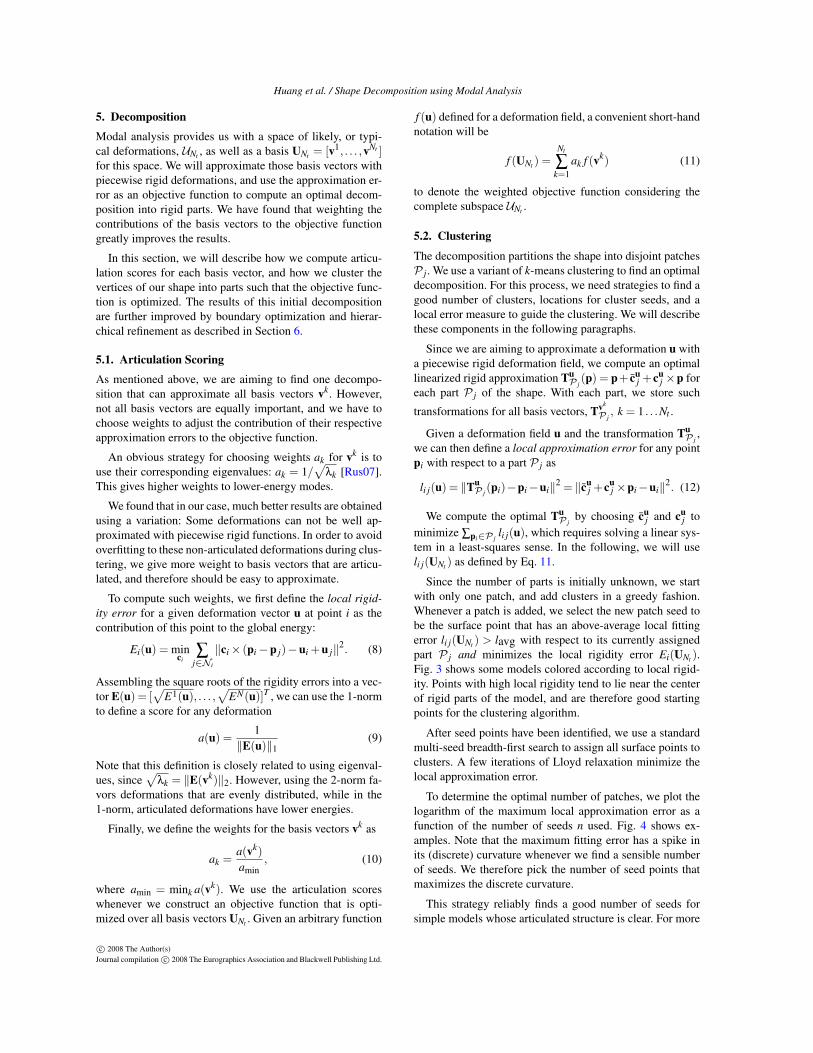
5.1. Articulation ScoringAs mentioned above, we are aiming to find one decompo-sition that can approximate all basis vectors vk. However,not all basis vectors are equally important, and we have tochoose weights to adjust the contribution of their respectiveapproximation errors to the objective function.

An obvious strategy for choosing weights ak for vk is touse their corresponding eigenvalues: ak = 1/

*"k [Rus07].

This gives higher weights to lower-energy modes.

We found that in our case, much better results are obtainedusing a variation: Some deformations can not be well ap-proximated with piecewise rigid functions. In order to avoidoverfitting to these non-articulated deformations during clus-tering, we give more weight to basis vectors that are articu-lated, and therefore should be easy to approximate.

To compute such weights, we first define the local rigid-ity error for a given deformation vector u at point i as thecontribution of this point to the global energy:

Ei(u) = minci

#j"Ni

#ci$ (pi%p j)%ui +u j#2. (8)

Assembling the square roots of the rigidity errors into a vec-tor E(u) = [

*E1(u), . . . ,

*EN(u)]T , we can use the 1-norm

to define a score for any deformation

a(u) =1

#E(u)#1(9)

Note that this definition is closely related to using eigenval-ues, since

*"k = #E(vk)#2. However, using the 2-norm fa-

vors deformations that are evenly distributed, while in the1-norm, articulated deformations have lower energies.

Finally, we define the weights for the basis vectors vk as

ak =a(vk)amin

, (10)

where amin = mink a(vk). We use the articulation scoreswhenever we construct an objective function that is opti-mized over all basis vectors UNt . Given an arbitrary function

f (u) defined for a deformation field, a convenient short-handnotation will be

f (UNt ) =Nt

#k=1

ak f (vk) (11)

to denote the weighted objective function considering thecomplete subspace UNt .

5.2. ClusteringThe decomposition partitions the shape into disjoint patchesP j. We use a variant of k-means clustering to find an optimaldecomposition. For this process, we need strategies to find agood number of clusters, locations for cluster seeds, and alocal error measure to guide the clustering. We will describethese components in the following paragraphs.

Since we are aiming to approximate a deformation u witha piecewise rigid deformation field, we compute an optimallinearized rigid approximation Tu

P j(p) = p+ cu

j +cuj $p for

each part P j of the shape. With each part, we store suchtransformations for all basis vectors, Tvk

P j, k = 1 . . .Nt .

Given a deformation field u and the transformation TuP j

,we can then define a local approximation error for any pointpi with respect to a part P j as

li j(u) = #TuP j (pi)%pi%ui#2 = #cu

j +cuj $pi%ui#2. (12)

We compute the optimal TuP j

by choosing cuj and cu

j tominimize #pi"P j li j(u), which requires solving a linear sys-tem in a least-squares sense. In the following, we will useli j(UNt ) as defined by Eq. 11.

Since the number of parts is initially unknown, we startwith only one patch, and add clusters in a greedy fashion.Whenever a patch is added, we select the new patch seed tobe the surface point that has an above-average local fittingerror li j(UNt ) > lavg with respect to its currently assignedpart P j and minimizes the local rigidity error Ei(UNt ).Fig. 3 shows some models colored according to local rigid-ity. Points with high local rigidity tend to lie near the centerof rigid parts of the model, and are therefore good startingpoints for the clustering algorithm.

After seed points have been identified, we use a standardmulti-seed breadth-first search to assign all surface points toclusters. A few iterations of Lloyd relaxation minimize thelocal approximation error.

To determine the optimal number of patches, we plot thelogarithm of the maximum local approximation error as afunction of the number of seeds n used. Fig. 4 shows ex-amples. Note that the maximum fitting error has a spike inits (discrete) curvature whenever we find a sensible numberof seeds. We therefore pick the number of seed points thatmaximizes the discrete curvature.

This strategy reliably finds a good number of seeds forsimple models whose articulated structure is clear. For more

c! 2008 The Author(s)Journal compilation c! 2008 The Eurographics Association and Blackwell Publishing Ltd.

Huang et al. / Shape Decomposition using Modal Analysis

Figure 3: The points in the models are colored accordingto local rigidity. The points with highest local rigidity (red)lie near the centers of rigid parts.

(a) (b)

Figure 4: The logarithm of the maximum local fitting er-ror (bottom graph) plotted against the number of patches,as well as the discrete curvature of the function (top graph).Good patch counts maximize the discrete curvature.

complicated models, the results can be ambiguous, eventhough all possibilities correspond to good segmentations.If no user guidance is available in an ambiguous case, wechoose the number of patches that is preceded by the biggestdecline in approximation error. Once hierarchical refinementis used, choosing the right number of patches become muchless important. Our experiments suggest that hierarchical re-finement leads to the same result independent of the numberof patches chosen in the initial iteration.

6. Patch OptimizationOnce we have obtained an initial decomposition, we opti-mize the parts further by considering deformations from UNt

that are optimized to be particularly useful in the region ofinterest. We use these fields for boundary optimization aswell as hierarchical refinement.

6.1. Locally Optimized Deformation FieldsGiven a region of interest I, we can compute a subspaceof UNt that contains the deformations that have low energycontent EI within I, while not considering their behavior inthe rest of the shape. As before, we can compute the HessianHI , which is simply a restriction of HP to vertices in I.

Analogous to computing the typical deformations of thecomplete shape, we now compute a subspace of the typi-cal deformations that have small deformation energy in I.

Since we are not choosing from the complete space of pos-sible deformations but from the subspace UNt , this leads to ageneralized eigenproblem

UTNt HIUNt x = %UT

Nt SIUNt x, (13)

Where the selection matrix SI = diag(&I)( I3 is a diagonalmatrix with zero entries for all points not in I.

As before, we obtain eigenvalues %k and eigenvectors xk.The eigenvectors in turn yield deformation vectors zk =UNt x

k, which we assemble into a matrix UI = [z1, . . . ,zNt ].

When using the locally optimized vector fields, we alsomodify the articulation weights ak to consider only rigiditywithin I.

6.2. Local Boundary OptimizationIn order to refine the boundaries between parts, we define akernel region K j and a support region R j for each part P j.Suppose the maximum local approximation error of points inP j is RP j = maxpi"P j li j(UNt ). We define the kernel regionas all points in P j whose local approximation error is small,

K j = {pi & P j | li j(UNt ) <RP j

4}. (14)

The support region R j is the largest contiguous set of pointsthat includes the kernel K j, and contains neither points thatare part of another kernel, nor points with a local approxima-tion error li j(UNt ) > 2RP j . We compute R j using breadth-first search.

The boundaries of patches are optimized for groups ofpatches whose support regions overlap. These are the small-est units that can be optimized independently. We start as-sembling patch groups by forming groups of two patches:Each pair of neighboring patches {Pi,P j}, where Ri )R j *= +, forms one group. If there is a three-way intersec-tion between patches Pi, P j, and Pk, i. e. Ri )R j )Rk *=+, we remove the two-element groups and add a group{Pi,P j,Pk}. This procedure is repeated for more complexintersections, although these are rare. An example of a patchgroup with 4 elements is shown in Fig. 5.

For each group G = {P j1 , . . . ,P j|G|}, we compute a ba-sis of locally optimal deformations UG as described in Sec-tion 6.1, and reapply the clustering method as described inSection 5.2 for all parts in G. This redefines the boundariesbetween parts in G, while leaving the rest of the segmenta-tion untouched. Fig. 5 shows an example of this process.

6.3. Hierarchical RefinementIt is straightforward to extend our algorithm to support hi-erarchical refinement. To refine a part P j, we compute lo-cally optimized typical deformations UP j as described inSection 6.1. We then continue with the segmentation pro-cedure as discussed in Section 5, restricting our operationsto P j only. Fig. 6 shows an example of hierarchical refine-ment on the dragon’s leg. For non-interactive processing, we

c! 2008 The Author(s)Journal compilation c! 2008 The Eurographics Association and Blackwell Publishing Ltd.

Huang et al. / Shape Decomposition using Modal Analysis

· · ·(a) (b) (c)

Figure 5: Optimizing the patch boundaries. (a) A group of4 patches before the optimization. The support regions of theleg, tail, and body patches overlap in the gray area; the ker-nels are colored red, blue, and gold. (b) Optimized local vec-tor fields are computed to determine the patch boundaries.(c) Result of the boundary optimization.

· · ·!

Figure 6: A leg of the dragon is refined using deformationfields optimized for this patch.

stop the hierarchical refinement when the smallest non-zeroeigenvalue %1 computed for a part P j is greater than thelargest initial eigenvalue computed for the complete shape,"Nt (note that as we restrict P j, %1 increases). Intuitively,this criterion stops processing when we cannot find vectorfields from UNt whose restriction to P j is interesting.

Since hierarchical refinement reuses the initial eigenvec-tors and applies a global termination criterion, the result ofhierarchical refinement is typically independent of the initialnumber of patches, making the “correct” number of patchesa much less critical parameter.

7. Skeleton Extraction

The decomposition extracted in the previous sections can beused to define a skeleton. Each part is associated with a boneof the skeleton. We will first discuss how to compute associ-ation weights, before we extract the skeleton structure.

7.1. Association Weights

Association weights determine how the rigid transforma-tions of the skeleton bones are interpolated onto the surface.In our case, the transformations are given for the kernel ofeach part. We compute weights w(P j,pi) that determine thecontribution of the rigid transformation given for the part P jto the transformation of pi. We choose these weights to belocal, such that only neighboring parts contribute to the de-formation of a surface point.

For each point pi, we define a set of neighboring partsG(pi) = {P j | pi &R j}, and compute locally optimized typ-ical deformation fields UG(pi).

We then find the association weights by minimizing thedifference between deformations created using the skele-ton and the typical vector fields. Given the (linearized) rigidtransformation Tu

K jthat minimizes the maximum local ap-

proximation error maxpi"K j li j(u) for some deformation u,we seek weights w(P j,pi) that minimize

#k

+++pi + zki %#

jw(P j,pi)Tzk

K j (pi)+++

2, (15)

subject to the positivity and partition of unity. This mini-mization can be solved efficiently as a quadratic program.

The resulting weights faithfully reproduce the locally op-timized vector fields. However, since the patch group asso-ciated with each point changes, there is no formal guaran-tee that the computed weights are smooth across the surface.Therefore, we apply a few steps of Laplacian smoothing, andrenormalize the weights.

7.2. Skeleton StructureWhile it is obvious that each part of the decompositionshould be associated with one bone of the skeleton, it isunclear what is the best joint structure connecting thesebones. We use the association weights to connect thosebones whose associated patches overlap most. To this end,we consider a weighted neighborhood graph of the decom-position. Each edge in this graph is weighted by

w(P j,Pk) =

,

#pi"P

w(P j,pi)w(Pk,pi)

-#1

. (16)

We then compute the joint structure of the skeleton as theminimum spanning tree (MST) of the weighted patch neigh-borhood graph.

We position each node of the MST with the barycenterof its associated kernel. Each edge in the MST is associ-ated with a joint, which is positioned at the barycenter ofthe boundary curve between the two parts connected by thisjoint. Fig. 8 shows skeletons for various models.

8. Results and DiscussionWe have tested our segmentation algorithm on various sur-face models. The results of the segmentations, as well as theextracted skeletons, are shown in Fig. 8. Table 1 summarizestiming and model statistics. All timings were measured ona 3.2 GHz PC with 2GB RAM. The total computation timeis clearly dominated by the eigen-decomposition of the Hes-sian. This decomposition has to be performed only once permodel, all other steps allow for interactive intervention.

Note that our method is applicable to noisy and even in-complete models. For demonstration purposes, we perturbedthe vertex positions of the Cow2 model by adding Gaussian

c! 2008 The Author(s)Journal compilation c! 2008 The Eurographics Association and Blackwell Publishing Ltd.

Huang et al. / Shape Decomposition using Modal Analysis

(a) (b)

(c) (d)

Figure 7: Robustness to noise and sampling. (a) Decom-position of a uniformly sampled version of the Cow2 model.(b) With noise and holes added. (c),(d) Irregular sampling.The right side is sampled more densely than the left. The re-sulting decomposition shows no appreciable differences tothe uniformly sampled version.

noise (with a variance equal to 1% of the model diagonal)in normal direction, and carved holes in the side of its body,head, and legs. As shown in Fig. 7, the segmentation is ro-bust against these modifications as long as the underlyingarticulated structure is not changed. We have also run the de-composition on a Cow2 model with varying sampling den-sity. As long as the energy is chosen appropriately, the sur-face sampling has no influence on the result.

The segmentation produced by our algorithm is also ro-bust to isometric and/or articulated deformations. The twoelephant models shown in Fig. 8 (a) have significantly dif-ferent poses, yet the computed segmentations are virtuallyidentical. This is to be expected since even though the defor-mation energy is non-linear, the deformation modes do nochange significantly after isometric deformations.

Fig. 8 (b) shows details of the decomposition of the Manmodel. The figure shows two possible initial decompositions(one with 5, one with 12 segments), as well as the final re-sult of hierarchical refinement. The hierarchical refinementconverges to the same solution independent of the numberof initial parts. This behavior is common, although we can-not give a formal guarantee due to the properties of the seedselection and clustering algorithm.

We have computed decompositions for the Horse and Manmodel, which we compare to segmentations obtained us-ing [LZ07], provided by the authors, as well as an implemen-tation of [KT03]. These segmentations are shown in Fig. 9.

Model N Nc tg tc tb th tw TCow1 11273 11 60.2 2.1 2.4 3.1 1.1 68.9Cow2 16914 8 96.2 1.1 3.1 — 2.1 102.5Dragon 22502 39 170.1 4.1 4.5 6.1 5.4 190.2Elephant1 20002 18 120.1 2.1 1.6 4.5 3.2 131.5Elephant2 20002 18 118.7 2.1 1.7 4.3 2.8 129.8Horse 19850 15 106.1 1.1 1.2 2.4 1.1 119.1Man 14603 32 80.4 2.2 2.3 1.7 2.5 89.1Raptor 22502 33 150.1 4.3 3.2 4.4 3.4 165.4

Table 1: Model statistics and computation times. Shownare the number of surface points N, the number of clustersNc, as well as computation times (in seconds) for the globaltypical vector fields tg, clustering tc, boundary refinement tb,hierarchical refinement th, association weight computationtw, and total time T .

(a) (b)

(c) (d) (e) (f)

Figure 9: (a) Segmentation of the Horse model using ourmethod. (b) Using [LZ07]. (c) Using [KT03]. (d) Segmenta-tion of the Man model using our method. (e) Using [LZ07].(f) Using [KT03]

Our method captures the articulated nature of the model.However, small features such as the horse’s ears are sepa-rated late in the refinement, since their geometric structuremakes them quite stable against deformations. Such featuresare more likely to be found by purely geometry-based algo-rithms, such as [LZ07].

If the desired result is not a decomposition based on thenatural deformations of an object, but one based on surfacetexture, or small surface features, our method is of only lim-ited use. Since our method finds a decomposition that bestapproximates the articulated nature of an object, the returneddecomposition in such cases might not correspond to logicalunits.

c! 2008 The Author(s)Journal compilation c! 2008 The Eurographics Association and Blackwell Publishing Ltd.

Huang et al. / Shape Decomposition using Modal Analysis

,

,

(a) (b)

Figure 8: (a) Decompositions and extracted skeletons for various surface models. Note that non-adjacent patches are distincteven if they share the same color. (b) The decomposition of the Man model. We can choose either 5 or 12 segments in the initialclustering step. In both cases, the hierarchical decomposition scheme terminates with the same result shown on the right.

9. Conclusion

We have presented a shape decomposition algorithm basedon optimal approximation of low-energy deformations. Themethod extracts the subspace of low-energy deformationsfor a given deformation energy. Using the information ob-tained by analyzing the typical deformations of the shape,we can compute meaningful shape decompositions usingonly a single pose, without resorting to heuristics based ongeometric features.

Our method is robust to noise and even small holes in theshape. It is therefore possible to apply it directly to scannedmodels. We believe our method will be very useful for rapidprototyping of animated models from real-world models, forexample clay models. Note also that the method is very gen-eral and can be computed to any surface, or even volumetricrepresentation, as long as an energy function and sensibleneighborhoods can be defined.

Using the skeletons extracted for each shape, it is possibleto perform deformation transfer between different models.To accomplish this, it would be necessary to obtain compat-ible skeletons for different models, with some isomorphismdescribing correspondences between joints and bones in ei-ther model. In the future, we will work on forcing a spe-cific skeleton layout in order to facilitate deformation trans-fer from another model.

Note that we have complete freedom in designing the de-formation energy. In all examples shown in this paper wehave used an energy definition that is uniform across the sur-face. A possible extension to our method would incorporateadditional knowledge about the structure of the surface intothe deformation energy, for example, by setting lower stiff-ness weights at joints.

AcknowledgmentsThis research was funded by the Max-Planck Center for Vi-sual Computing and Communication, as well as NSF grantsITR 0205671 and FRG 0354543, NIH grant GM-072970,and DARPA grant HR0011-05-1-0007. Qi-xing Huang issupported by the Mr. and Mrs. Chin-Nan Chen StanfordGraduate Fellowship. Bart Adams is funded by the Fundfor Scientific Research, Flanders (F.W.O.-Vlaanderen). Wewould like to thank the Stanford University and Aim@Shapefor providing various models, and the anonymous reviewersfor their helpful comments.

References[ATC"08] AU O. K.-C., TAI C.-L., CHU H.-K., COHEN-OR

D., LEE T.-Y.: Skeleton Extraction by Mesh Contraction. ACMTransactions on Graphics 27, 3 (2008).

[BJ05] BARBIC J., JAMES D. L.: Real-Time subspace integrationfor St. Venant-Kirchhoff deformable models. ACM Transactionson Graphics 24, 3 (2005), 982–990.

[BP07] BARAN I., POPOVIC J.: Automatic rigging and animationof 3D characters. ACM Transactions on Graphics 26, 3 (2007),72.

[CK05] CHOI M. G., KO H.-S.: Modal Warping: Real-TimeSimulation of Large Rotational Deformation and Manipulation.IEEE Transactions on Visualization and Computer Graphics 11(2005), 91–101.

[CSAD04] COHEN-STEINER D., ALLIEZ P., DESBRUN M.:Variational shape approximation. 905–914.

[dGGV08] DE GOES F., GOLDENSTEIN S., VELHO L.: A Hi-erarchical Segmentation of Articulated Bodies. In EurographicsSymposium on Geometry Processing (SGP) (2008).

[FKS"04] FUNKHOUSER T., KAZHDAN M., SHILANE P., MINP., KIEFER W., TAL A., RUSINKIEWICZ S., DOBKIN D.: Mod-

c! 2008 The Author(s)Journal compilation c! 2008 The Eurographics Association and Blackwell Publishing Ltd.

Huang et al. / Shape Decomposition using Modal Analysis

eling by example. ACM Transactions on Graphics 23, 3 (2004),652–663.

[GCO06] GAL R., COHEN-OR D.: Salient geometric featuresfor partial shape matching and similarity. ACM Transactions onGraphics 25, 1 (2006), 130–150.

[GG04] GELFAND N., GUIBAS L. J.: Shape Segmentation UsingLocal Slippage Analysis. In Symposium on Geometry Processing(2004), pp. 219–228.

[GHDS03] GRINSPUN E., HIRANI A. N., DESBRUN M.,SCHRÖDER P.: Discrete shells. In Symposium on Computer An-imation (2003), pp. 62–67.

[HOP"05] HOFER M., ODEHNAL B., POTTMANN H., STEINERT., WALLNER J.: 3D shape recognition and reconstruction basedon line element geometry. In IEEE International Conference onComputer Vision (2005), vol. 2, pp. 1532–1538.

[JP02] JAMES D., PAI D.: DyRT: Dynamic Response Texturesfor Real Time Deformation Simulation With Graphics Hardware.ACM Transactions on Graphics 21, 3 (2002), 582–585.

[JT05] JAMES D. L., TWIGG C. D.: Skinning mesh animations.ACM Transactions on Graphics 24, 3 (2005), 399–407.

[KJS07] KREAVOY V., JULIUS D., SHEFFER A.: Model Compo-sition from Interchangeable Components. In 15th Pacific Conf.on Computer Graphics and Appl. (2007), pp. 129–138.

[KLT05] KATZ S., LEIFMAN G., TAL A.: Mesh Segmentationusing Feature Point and Core Extraction. The Visual Computer(Pacific Graph.) 21, 8-10 (2005), 649–658.

[KMP07] KILIAN M., MITRA N. J., POTTMANN H.: GeometricModeling in Shape Space. ACM Transactions on Graphics 26, 3(2007), 1–8.

[KT03] KATZ S., TAL A.: Hierarchical mesh decomposition us-ing fuzzy clustering and cuts. ACM Transactions on Graphics22, 3 (2003), 954–961.

[LKA06] LIEN J.-M., KEYSER J., AMATO N. M.: Simultaneousshape decomposition and skeletonization. In Proc. of the 2006ACM Symp. on solid and physical modeling (2006), pp. 219–228.

[LLS"05] LEE Y., LEE S., SHAMIR A., COHEN-OR D., SEI-DEL H.-P.: Mesh scissoring with minima rule and part salience.Comp. Aided Geometric Design 22, 5 (2005), 444–465.

[LZ07] LIU R., ZHANG H.: Mesh Segmentation via Spectral Em-bedding and Contour Analysis. Computer Graphics Forum 26, 3(2007), 385–394.

[LZHM06] LAI Y.-K., ZHOU Q.-Y., HU S.-M., MARTIN R. R.:Feature sensitive mesh segmentation. In Symposium on Solid andPhysical Modeling (2006), pp. 17–25.

[MPS"04] MORTARA M., PATANÈ G., SPAGNUOLO M., FALCI-DIENO B., ROSSIGNAC J.: Plumber: a method for a multi-scaledecomposition of 3D shapes into tubular primitives and bod-ies. In Proceedings of Solid Modeling and Applications (2004),pp. 339–344.

[PW89] PENTLAND A., WILLIAMS J.: Good vibrations: modaldynamics for graphics and animation. In Proceedings of ACMSIGGRAPH 89 (1989), pp. 215–222.

[Rus07] RUSTAMOV R. M.: Laplace-Beltrami eigenfunctions fordeformation invariant shape representation. In Symposium on Ge-ometry Processing (2007), pp. 225–233.

[SA07] SORKINE O., ALEXA M.: As-rigid-as-possible sur-face modeling. In Symposium on Geometry Processing (2007),pp. 109–116.

[Sha06] SHAMIR A.: Segmentation and Shape Extraction of 3DBoundary Meshes. In Eurographics 2006 - State of the Art Re-ports (2006), pp. 137–149.

[SP95] SCLAROFF S., PENTLAND A.: Modal Matching for Cor-respondence and Recognition. IEEE Transactions on PatternAnalysis and Machine Intelligence 17, 6 (1995), 545–561.

[SSCO08] SHAPIRA L., SHAMIR A., COHEN-OR D.: Consistentmesh partitioning and skeletonisation using the shape diameterfunction. Visual Computer 24, 4 (2008), 249–259.

[SY07] SCHAEFER S., YUKSEL C.: Example-based skeleton ex-traction. In Symposium on Geometry Processing (2007), pp. 153–162.

[SZT"07] SHI X., ZHOU K., TONG Y., DESBRUN M., BAO H.,GUO B.: Mesh puppetry: cascading optimization of mesh defor-mation with inverse kinematics. ACM Transactions on Graphics26, 3 (2007), 81.

[Wei99] WEISS Y.: Segmentation Using Eigenvectors: A Unify-ing View. In Proc. ICCV (1999), pp. 975–982.

[WK05] WU J., KOBBELT L.: Structure Recovery via HybridVariational Surface Approximation. Computer Graphics Forum24, 3 (2005), 277–284.

[YLL"05] YAMAUCHI H., LEE S., LEE Y., OHTAKE Y.,BELYAEV A., SEIDEL H.-P.: Feature Sensitive Mesh Segmen-tation with Mean Shift. In Shape Modeling and Applications(2005), pp. 238–245.

[YLW06] YAN D.-M., LIU Y., WANG W.: Quadric Surface Ex-traction by Variational Shape Approximation. In Geometric Mod-eling and Processing (2006), pp. 73–86.

Appendix A: Derivation for Eq. 2

Given a function g(x) = miny f (x,y), and define y(x) =argminy f (x,y) such that g(x) = f (x,y(x)).

We observe that by definition, !f!y (x,y(x)) = 0, for all x.

This means in particular that

!!x

%! f!y (x,y(x))

&=

!2 f!y!x (x,y(x))+

!2 f!y2 (x) · !y

!x (x) = 0

(17)and we can therefore express !y

!x (x) as

!y!x (x) =%

,!2 f!y2 (x,y(x))

-#1

· !2 f!y!x (x,y(x)). (18)

Using the chain rule, and using (17) and (18), we can ex-pand the Hessian of g as

!2g!x2 (x) = !2

!x2 [ f (x,y(x))]

= !2 f!x2 (x,y(x))+ !2 f

!x!y (x,y(x))· !y!x (x)

= !2 f!x2 (x,y(x))# !2 f

!x!y (x,y(x))·!

!2 f!y2 (x,y(x))

"!1· !2 f

!y!x (x,y(x)).

c! 2008 The Author(s)Journal compilation c! 2008 The Eurographics Association and Blackwell Publishing Ltd.