shallow landslide models: a probabilistic approach arXiv ... · 2 S. Raia et al.: Improving...
25
Manuscript prepared for Geosci. Model Dev. with version 5.0 of the L A T E X class copernicus.cls. Date: 9 April 2018 Improving predictive power of physically based rainfall-induced shallow landslide models: a probabilistic approach S. Raia 1 , M. Alvioli 1 , M. Rossi 1 , R. L. Baum 2 , J. W. Godt 2 , and F. Guzzetti 1 1 CNR IRPI, via Madonna Alta 126, 06128 Perugia, Italy 2 US Geological Survey, P.O. Box 25046, Mail Stop 966, Denver, CO 80225-0046, USA Correspondence to: M. Alvioli ([email protected]) Abstract. Distributed models to forecast the spatial and temporal occurrence of rainfall-induced shallow landslides are based on deterministic laws. These models extend spa- tially the static stability models adopted in geotechnical en- gineering, and adopt an infinite-slope geometry to balance the resisting and the driving forces acting on the sliding mass. An infiltration model is used to determine how rain- fall changes pore-water conditions, modulating the local sta- bility/instability conditions. A problem with the operation of the existing models lays in the difficulty in obtaining accu- rate values for the several variables that describe the ma- terial properties of the slopes. The problem is particularly severe when the models are applied over large areas, for which sufficient information on the geotechnical and hy- drological conditions of the slopes is not generally avail- able. To help solve the problem, we propose a probabilistic Monte Carlo approach to the distributed modeling of rainfall- induced shallow landslides. For the purpose, we have mod- ified the Transient Rainfall Infiltration and Grid-Based Re- gional Slope-Stability Analysis (TRIGRS) code. The new code (TRIGRS-P) adopts a probabilistic approach to com- pute, on a cell-by-cell basis, transient pore-pressure changes and related changes in the factor of safety due to rainfall in- filtration. Infiltration is modeled using analytical solutions of partial differential equations describing one-dimensional vertical flow in isotropic, homogeneous materials. Both sat- urated and unsaturated soil conditions can be considered. TRIGRS-P copes with the natural variability inherent to the mechanical and hydrological properties of the slope materi- als by allowing values of the TRIGRS model input param- eters to be sampled randomly from a given probability dis- tribution. The range of variation and the mean value of the parameters can be determined by the usual methods used for preparing the TRIGRS input parameters. The outputs of sev- eral model runs obtained varying the input parameters are an- alyzed statistically, and compared to the original (determinis- tic) model output. The comparison suggests an improvement of the predictive power of the model of about 10 % and 16 % in two small test areas i.e., i.e., the Frontignano (Italy) and the Mukilteo (USA) areas. We discuss the computational re- quirements of TRIGRS-P to determine the potential use of the numerical model to forecast the spatial and temporal oc- currence of rainfall-induced shallow landslides in very large areas, extending for several hundreds or thousands of square kilometers. Parallel execution of the code using a simple pro- cess distribution and the Message Passing Interface (MPI) on multi-processor machines was successful, opening the possi- bly of testing the use of TRIGRS-P for the operational fore- casting of rainfall-induced shallow landslides over large re- gions. 1 Introduction Rainfall is a primary trigger of landslides, and rainfall- induced landslides are common in many physiographical en- vironments, e.g. Brabb and Harrod (1989). Prediction of the location and time of occurrence of shallow rainfall-induced landslides remains a difficult task, which can be accom- plished adopting empirical (Crosta, 1998; Sirangelo et al., 2003; Aleotti, 2004; Guzzetti et al., 2007, 2008), statistical (Soeters and Van Westen, 1996; Guzzetti et al., 1999, 2005, 2006a; Committee on the Review of the National Landslide Hazards Mitigation Strategy, 2004), or process based (Mont- gomery and Dietrich, 1994; Terlien, 1998; Baum et al., 2002, 2008, 2010; Crosta and Frattini, 2003; Simoni et al., 2008; Godt et al., 2008; Vieira et al., 2010) approaches, or a com- bination of them (Gorsevski et al., 2006; Frattini et al., 2009). Inspection of the literature, reveals that process based (deter- ministic, physically based) models are preferred to forecast arXiv:1305.4803v2 [physics.geo-ph] 14 Mar 2014
Transcript of shallow landslide models: a probabilistic approach arXiv ... · 2 S. Raia et al.: Improving...
Manuscript prepared for Geosci. Model Dev.with version 5.0 of the LATEX class copernicus.cls.Date: 9 April 2018
Improving predictive power of physically based rainfall-inducedshallow landslide models: a probabilistic approachS. Raia1, M. Alvioli1, M. Rossi1, R. L. Baum2, J. W. Godt2, and F. Guzzetti11CNR IRPI, via Madonna Alta 126, 06128 Perugia, Italy2US Geological Survey, P.O. Box 25046, Mail Stop 966, Denver, CO 80225-0046, USA
Correspondence to: M. Alvioli ([email protected])
Abstract. Distributed models to forecast the spatial andtemporal occurrence of rainfall-induced shallow landslidesare based on deterministic laws. These models extend spa-tially the static stability models adopted in geotechnical en-gineering, and adopt an infinite-slope geometry to balancethe resisting and the driving forces acting on the slidingmass. An infiltration model is used to determine how rain-fall changes pore-water conditions, modulating the local sta-bility/instability conditions. A problem with the operation ofthe existing models lays in the difficulty in obtaining accu-rate values for the several variables that describe the ma-terial properties of the slopes. The problem is particularlysevere when the models are applied over large areas, forwhich sufficient information on the geotechnical and hy-drological conditions of the slopes is not generally avail-able. To help solve the problem, we propose a probabilisticMonte Carlo approach to the distributed modeling of rainfall-induced shallow landslides. For the purpose, we have mod-ified the Transient Rainfall Infiltration and Grid-Based Re-gional Slope-Stability Analysis (TRIGRS) code. The newcode (TRIGRS-P) adopts a probabilistic approach to com-pute, on a cell-by-cell basis, transient pore-pressure changesand related changes in the factor of safety due to rainfall in-filtration. Infiltration is modeled using analytical solutionsof partial differential equations describing one-dimensionalvertical flow in isotropic, homogeneous materials. Both sat-urated and unsaturated soil conditions can be considered.TRIGRS-P copes with the natural variability inherent to themechanical and hydrological properties of the slope materi-als by allowing values of the TRIGRS model input param-eters to be sampled randomly from a given probability dis-tribution. The range of variation and the mean value of theparameters can be determined by the usual methods used forpreparing the TRIGRS input parameters. The outputs of sev-eral model runs obtained varying the input parameters are an-
alyzed statistically, and compared to the original (determinis-tic) model output. The comparison suggests an improvementof the predictive power of the model of about 10 % and 16 %in two small test areas i.e., i.e., the Frontignano (Italy) andthe Mukilteo (USA) areas. We discuss the computational re-quirements of TRIGRS-P to determine the potential use ofthe numerical model to forecast the spatial and temporal oc-currence of rainfall-induced shallow landslides in very largeareas, extending for several hundreds or thousands of squarekilometers. Parallel execution of the code using a simple pro-cess distribution and the Message Passing Interface (MPI) onmulti-processor machines was successful, opening the possi-bly of testing the use of TRIGRS-P for the operational fore-casting of rainfall-induced shallow landslides over large re-gions.
1 Introduction
Rainfall is a primary trigger of landslides, and rainfall-induced landslides are common in many physiographical en-vironments, e.g. Brabb and Harrod (1989). Prediction of thelocation and time of occurrence of shallow rainfall-inducedlandslides remains a difficult task, which can be accom-plished adopting empirical (Crosta, 1998; Sirangelo et al.,2003; Aleotti, 2004; Guzzetti et al., 2007, 2008), statistical(Soeters and Van Westen, 1996; Guzzetti et al., 1999, 2005,2006a; Committee on the Review of the National LandslideHazards Mitigation Strategy, 2004), or process based (Mont-gomery and Dietrich, 1994; Terlien, 1998; Baum et al., 2002,2008, 2010; Crosta and Frattini, 2003; Simoni et al., 2008;Godt et al., 2008; Vieira et al., 2010) approaches, or a com-bination of them (Gorsevski et al., 2006; Frattini et al., 2009).Inspection of the literature, reveals that process based (deter-ministic, physically based) models are preferred to forecast
arX
iv:1
305.
4803
v2 [
phys
ics.
geo-
ph]
14
Mar
201
4
2 S. Raia et al.: Improving landslide modeling
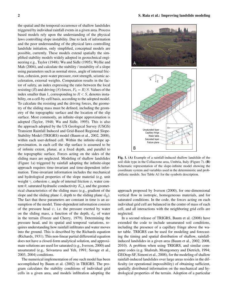
the spatial and the temporal occurrence of shallow landslidestriggered by individual rainfall events in a given area. Processbased models rely upon the understanding of the physicallaws controlling slope instability. Due to lack of informationand the poor understanding of the physical laws controllinglandslide initiation, only simplified, conceptual models arepossible, currently. These models extend spatially the sim-plified stability models widely adopted in geotechnical engi-neering e.g., Taylor (1948); Wu and Sidle (1995); Wyllie andMah (2004), and calculate the stability / instability of a slopeusing parameters such as normal stress, angle of internal fric-tion, cohesion, pore-water pressure, root strength, seismic ac-celeration, external weights. Computation results in the fac-tor of safety, an index expressing the ratio between the localresisting (R) and driving (S) forces, FS =R/S. Values of theindex smaller than 1, corresponding to R< S, denotes insta-bility, on a cell-by-cell basis, according to the adopted model.To calculate the resisting and the driving forces, the geome-try of the sliding mass must be defined, including the geom-etry of the topographic surface and the location of the slipsurface. Most commonly, an infinite-slope approximation isadopted (Taylor, 1948; Wu and Sidle, 1995). This is alsothe approach adopted by the US Geological Survey (USGS)Transient Rainfall Induced and Grid-Based Regional Slope-Stability Model (TRIGRS) model (Baum et al., 2002, 2008),within each user-defined cell. Within the infinite-slope ap-proximation, in each cell the slip surface is assumed to beof infinite extent, planar, at a fixed depth, and parallel tothe topographic surface. Forces acting on the sides of thesliding mass are neglected. Modeling of shallow landslides(Figure 1a) triggered by rainfall adopting the infinite-slopeapproach requires time-invariant and time-dependent infor-mation. Time-invariant information includes the mechanicaland hydrological properties of the slope material (e.g. unitweight γ, cohesion c, angle of internal friction φ, water con-tent θ, saturated hydraulic conductivity Ks), and the geomet-rical characteristics of the sliding mass (e.g., gradient of theslope and the sliding plane δ, depth to the sliding plane dfp).The fact that these parameters are constant in time is an as-sumption of the model. Time-dependent information consistsof the pressure head ψ, i.e. the pressure exerted by wateron the sliding mass, a function of the depth, dw of waterin the terrain (Freeze and Cherry, 1979). Determining thepressure head, and its spatial and temporal variations, re-quires understanding how rainfall infiltrates and water movesinto the ground. This is described by the Richards equation(Richards, 1931). This non-linear partial differential equationdoes not have a closed-form analytical solution, and approxi-mate solutions are used for saturated (e.g., Iverson, 2000) andunsaturated (e.g,. Srivastava and Yeh, 1991; Savage et al.,2003, 2004) conditions.
The numerical implementation of one such model has beenaccomplished by Baum et al. (2002) in TRIGRS. The pro-gram calculates the stability conditions of individual gridcells in a given area, and models infiltration adopting the
Capillary fringeUnsaturated layer
Water tableSaturated layer
Failure plane
X
Zδ z
du
dw dfp
XZ
Y
A
B
Fig. 1. (A) Example of a rainfall-induced shallow landslide of thesoil slide type in the Collazzone area, Umbria, Italy (Figure 7). (B)Schematic representation of the slope-infinite model showing thecoordinate system and variables used in the deterministic and prob-abilistic models. See Table A1 for the symbols description.
approach proposed by Iverson (2000), for one-dimensionalvertical flow in isotropic, homogeneous materials, and forsaturated conditions. In the code, the forces acting on eachindividual grid cell are balanced in the centre of mass of eachcell, and all interactions with the neighboring grid cells areneglected.
In a second release of TRIGRS, Baum et al. (2008) haveextended the code to include unsaturated soil conditions,including the presence of a capillary fringe above the wa-ter table. TRIGRS can be used for modeling and forecast-ing the timing and spatial distribution of shallow, rainfall-induced landslides in a given area (Baum et al., 2002, 2008,2010). A problem when using TRIGRS, and similar com-puter codes (e.g. Shalstab, Montgomery and Dietrich, 1994;GEOtop-SF, Simoni et al., 2008), for the modeling of shallowrainfall-induced landslides over large areas resides in the dif-ficulty (or operational impossibility) of obtaining sufficient,spatially distributed information on the mechanical and hy-drological properties of the terrain. Adoption of a particular
S. Raia et al.: Improving landslide modeling 3
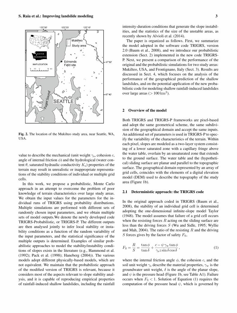
Fig. 2. The location of the Mukilteo study area, near Seattle, WA,USA.
value to describe the mechanical (unit weight γs, cohesion c,angle of internal friction φ) and the hydrological (water con-tent θ, saturated hydraulic conductivity Ks) properties of theterrain may result in unrealistic or inappropriate representa-tions of the stability conditions of individual or multiple gridcells.
In this work, we propose a probabilistic, Monte Carloapproach in an attempt to overcome the problem of poorknowledge of terrain characteristics over large study areas.We obtain the input values for the parameters for the in-dividual runs of TRIGRS using probability distributions.Multiple simulations are performed with different sets ofrandomly chosen input parameters, and we obtain multiplesets of model outputs.We denote the newly developed codeTRIGRS-Probabilistic, or TRIGRS-P. The different outputsare then analysed jointly to infer local stability or insta-bility conditions as a function of the random variability ofthe input parameters, and the statistical significance of themultiple outputs is determined. Examples of similar prob-abilistic approaches to model the stability/instability condi-tions of slopes exists in the literature (e.g., Hammond et al.(1992); Pack et al. (1998); Haneberg (2004)). The variousmodels adopt different physically-based models, which arenot equivalent. We maintain that the probabilistic approachof the modified version of TRIGRS is relevant, because itconsiders most of the aspects relevant to slope stability anal-ysis, and it is capable of reproducing empirical propertiesof rainfall-induced shallow landslides, including the rainfall
intensity-duration conditions that generate the slope instabil-ities, and the statistics of the size of the unstable areas, asrecently shown by Alvioli et al. (2014).
The paper is organized as follows. First, we summarizethe model adopted in the software code TRIGRS, version2.0 (Baum et al., 2008), and we introduce our probabilisticextension (Sect. 2) implemented in the new code TRIGRS-P. Next, we present a comparison of the performance of theoriginal and the probabilistic simulations for two study areas:Mukilteo, USA, and Frontignano, Italy (Sect. 3). Results arediscussed in Sect. 4, which focuses on the analysis of theperformance of the geographical prediction of the shallowlandslides, and on the potential application of the new proba-bilistic code for modeling shallow rainfall-induced landslidesover large areas (> 100 km2).
2 Overview of the model
Both TRIGRS and TRIGRS-P frameworks are pixel-basedand adopt the same geometrical scheme, the same subdivi-sion of the geographical domain and accept the same inputs.An additional set of parameters is used in TRIGRS-P to spec-ify the variability of the characteristics of the terrain. Withineach pixel, slopes are modeled as a two-layer system consist-ing of a lower saturated zone with a capillary fringe abovethe water table, overlain by an unsaturated zone that extendsto the ground surface. The water table and the (hypotheti-cal) sliding surface are planar and parallel to the topographicsurface. The geographical domain represented by an array ofgrid cells, coincides with the elements of a digital elevationmodel (DEM) used to describe the topography of the studyarea (Figure 1b).
2.1 Deterministic approach: the TRIGRS code
In the original approach coded in TRIGRS (Baum et al.,2008), the stability of an individual grid cell is determinedadopting the one-dimensional infinite-slope model Taylor(1948). The model assumes that failure of a grid cell occurswhen the resisting forces R acting on the sliding surface areless than the driving forces S (Wu and Sidle, 1995; Wyllieand Mah, 2004). The ratio of the resisting R and the drivingS forces gives by the factor of safety FS,
FS =R
S=
tanφ
tanδ+c−ψγw tanφ
γsz sinδ cosδ, (1)
where the internal friction angle φ, the cohesion c, and thesoil unit weight γs describe the material properties, γw is thegroundwater unit weight, δ is the angle of the planar slope,and ψ is the pressure head (Figure 1b, see Table A1). Failureoccurs when FS < 1. Solution of Equation (1) requires thecomputation of the pressure head ψ, which is governed by
4 S. Raia et al.: Improving landslide modeling
1278000 1280000
3440
0034
6000
3400
0034
2000
3430
0034
5000
3390
0034
1000
1277000 1279000
A
1278000 1280000
3440
0034
6000
3400
0034
2000
3430
0034
5000
3390
0034
1000
1277000 1279000
B
1278000 1280000
3430
0034
5000
3390
0034
1000
3430
0034
5000
3390
0034
1000
1277000 1279000
C
Qvt
Qva
Qtb
1278000 1280000
3440
0034
6000
3400
0034
2000
3430
0034
5000
3390
0034
1000
1277000 1279000
D
1278000 128000034
4000
3460
0034
0000
3420
00
3430
0034
5000
3390
0034
1000
1277000 1279000
E
1278000 1280000
3440
0034
6000
3400
0034
2000
3430
0034
5000
3390
0034
1000
1277000 1279000
F
0°
90° 79.5
6.0
10.4
4.1
TP
FPTN
FN
56.1
3.0
33.8
7.1
TP
FPTN
FN
Factor of safety, Fs≤ 0.7
(0.7, 0.8]
(0.8, 0.9]
(0.9, 1.0]
(1.0, 1.1]
(1.1, 1.2]
(1.2, 1.3]
(1.3, 1.4]
(1.4, 1.5]
> 1.5
Factor of safety, Fs≤ 0.7
(0.7, 0.8]
(0.8, 0.9]
(0.9, 1.0]
(1.0, 1.1]
(1.1, 1.2]
(1.2, 1.3]
(1.3, 1.4]
(1.4, 1.5]
> 1.5
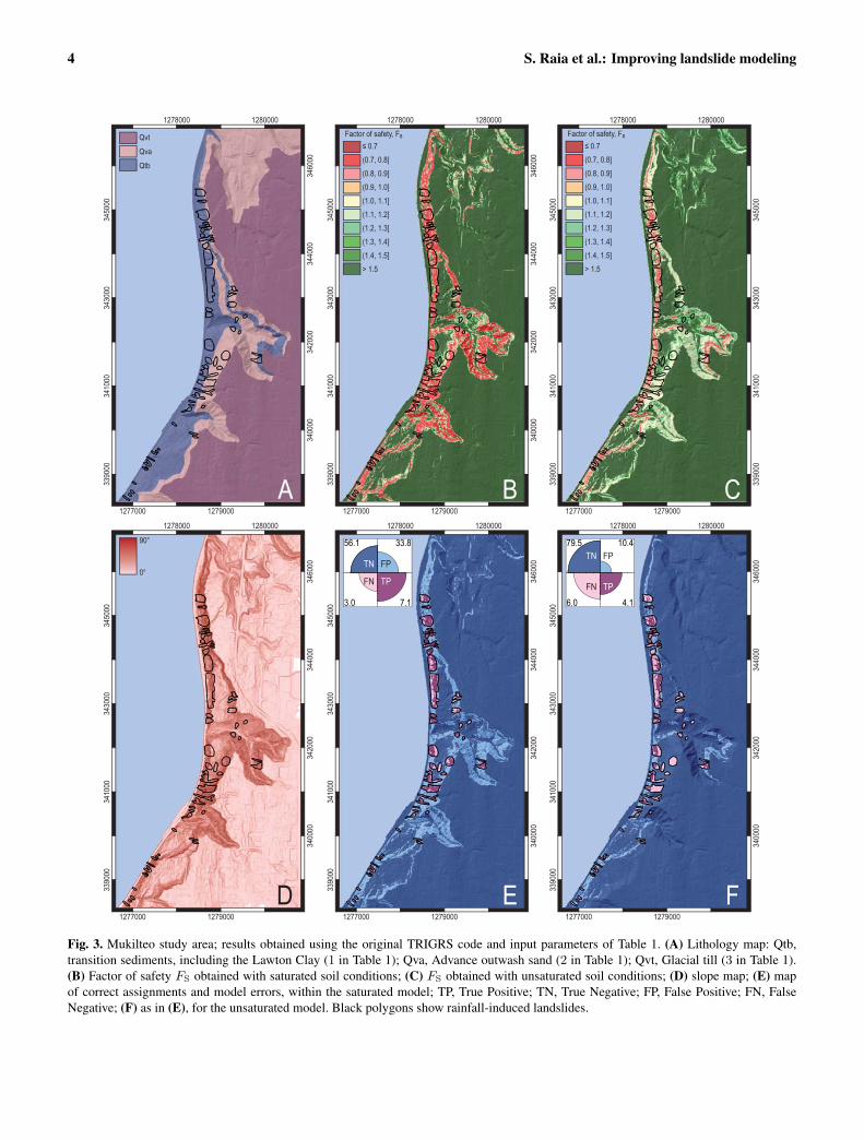
Fig. 3. Mukilteo study area; results obtained using the original TRIGRS code and input parameters of Table 1. (A) Lithology map: Qtb,transition sediments, including the Lawton Clay (1 in Table 1); Qva, Advance outwash sand (2 in Table 1); Qvt, Glacial till (3 in Table 1).(B) Factor of safety FS obtained with saturated soil conditions; (C) FS obtained with unsaturated soil conditions; (D) slope map; (E) mapof correct assignments and model errors, within the saturated model; TP, True Positive; TN, True Negative; FP, False Positive; FN, FalseNegative; (F) as in (E), for the unsaturated model. Black polygons show rainfall-induced landslides.
S. Raia et al.: Improving landslide modeling 5
1278000 1280000
3440
0034
6000
3400
0034
2000
3430
0034
5000
3390
0034
1000
1277000 1279000
B
1278000 1280000
3430
0034
5000
3390
0034
1000
3430
0034
5000
3390
0034
1000
1277000 1279000
C
1278000 1280000
3440
0034
6000
3400
0034
2000
3430
0034
5000
3390
0034
1000
1277000 1279000
A1278000 1280000
3440
0034
6000
3400
0034
2000
3430
0034
5000
3390
0034
1000
1277000 1279000
E
1278000 1280000
3430
0034
5000
3390
0034
1000
3430
0034
5000
3390
0034
1000
1277000 1279000
F
1278000 1280000
3440
0034
6000
3400
0034
2000
3430
0034
5000
3390
0034
1000
1277000 1279000
D
λ=0.01
ν=0.8
λ=0.5 λ=1.0
ν=1.1ν=0.9
0.7 0.8 0.9 1.0 1.1 1.2 1.3 1.4 1.5Factor of safety, Fs
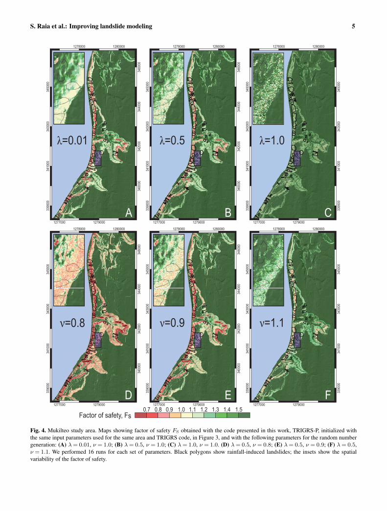
Fig. 4. Mukilteo study area. Maps showing factor of safety FS obtained with the code presented in this work, TRIGRS-P, initialized withthe same input parameters used for the same area and TRIGRS code, in Figure 3, and with the following parameters for the random numbergeneration: (A) λ= 0.01, ν = 1.0; (B) λ= 0.5, ν = 1.0; (C) λ= 1.0, ν = 1.0. (D) λ= 0.5, ν = 0.8; (E) λ= 0.5, ν = 0.9; (F) λ= 0.5,ν = 1.1. We performed 16 runs for each set of parameters. Black polygons show rainfall-induced landslides; the insets show the spatialvariability of the factor of safety.
6 S. Raia et al.: Improving landslide modeling
1278000 1280000
344000
346000
340000
342000
343000
345000
339000
341000
1277000 1279000
B
1278000 1280000
344000
346000
340000
342000
343000
345000
339000
341000
1277000 1279000
A
1278000 1280000
344000
346000
340000
342000
343000
345000
339000
341000
1277000 1279000
C1278000 1280000
344000
346000
340000
342000
343000
345000
339000
341000
1277000 1279000
E
1278000 1280000
344000
346000
340000
342000
343000
345000
339000
341000
1277000 1279000
D
1278000 1280000
344000
346000
340000
342000
343000
345000
339000
341000
1277000 1279000
F
λ=0.01
ν=0.8
λ=0.5 λ=1.0
ν=1.1ν=0.9
79.5
6.0
10.4
4.1
TP
FPTN
FN
49.0
2.4
40.9
7.7
TPFPTN
FN
69.2
4.4
20.7
5.7
TPFPTN
FN
84.9
7.8
5.0
2.3TP
FPTN
FN
79.4
6.0
10.5
4.1
TP
FPTN
FN
79.3
6.1
10.6
4.0
TP
FPTN
FN
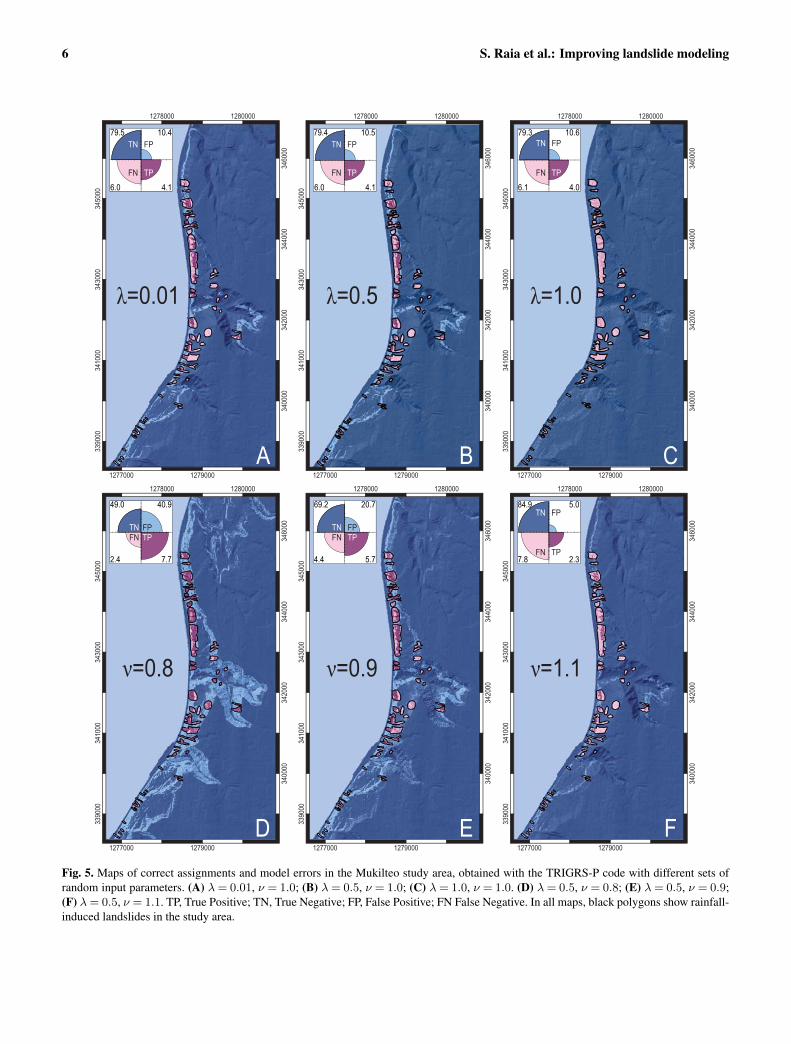
Fig. 5. Maps of correct assignments and model errors in the Mukilteo study area, obtained with the TRIGRS-P code with different sets ofrandom input parameters. (A) λ= 0.01, ν = 1.0; (B) λ= 0.5, ν = 1.0; (C) λ= 1.0, ν = 1.0. (D) λ= 0.5, ν = 0.8; (E) λ= 0.5, ν = 0.9;(F) λ= 0.5, ν = 1.1. TP, True Positive; TN, True Negative; FP, False Positive; FN False Negative. In all maps, black polygons show rainfall-induced landslides in the study area.
S. Raia et al.: Improving landslide modeling 7
the Richards (1931) equation:
∂
∂z
[Kz (ψ)
∂ (ψ− z)∂z
]=∂θ
∂t, (2)
where, z is the slope-normal coordinate, t is the time, Kz
is the vertical hydraulic conductivity that depends on thepressure head ψ, and θ is the volumetric water content (Fig-ure 1b). Equation (2) is solved in TRIGRS adopting the mod-eling scheme proposed by Baum et al. (2008).
For saturated conditions, TRIGRS uses a modified versionof the analytical solutions of Equation (2) proposed by Iver-son (2000), for short term and for long-term rainfall periods.Again, the modification consists chiefly in the possibility ofusing a complex rainfall history (Baum et al., 2008). To lin-earize Equation (2), Iverson (2000) adopted a normalizationcriterion using a length scale ratio as follows:
ε=
√d2
fp/D0
A/D0=
dfp√A, (3)
whereD0 is the maximum hydraulic diffusivity,A is the con-tributing area that affects hydraulic pressure at the potentialfailure plane depth dfp, and d2
fp/D0 and A/D0 are the mini-mum time required for slope-normal (d2
fp/D0) and for slope-lateral (A/D0) pore pressure transmission (see Table A1).Under the condition ε� 1, simplification of Equation (2)gives (Iverson, 2000):
∂
∂z∗
[K∗(ψ)
(∂ψ∗
∂z∗− z∗
)]= 0 , for t >
A
D0(4)
and
∂
∂z∗
[K∗(∂ψ∗∂z∗− z∗
)]=C(ψ)
C0
∂ψ∗∂t∗
, for t� A
D0, (5)
where ψ∗ = ψ/dfp, t∗ = tD/A , and z∗ = z/√dfp.
For unsaturated conditions, the code uses a modified ver-sion of the analytical solution of Equation (2) proposed bySrivastava and Yeh (1991), for the case of one-dimensional,transient, vertical infiltration. The modification consists inthe use of a variable rainfall history (intensity, duration), al-lowing modeling of complex rainfall patterns (Baum et al.,2008). Equation (2) was linearized in Srivastava and Yeh(1991), who adopted the following exponential model (Gard-ner, 1958):
Kz (ψ) =Ks eαψ ; (6)
θ = θr + (θs− θr) eαψ , (7)
where Ks is the saturated hydraulic conductivity, θr is theresidual water content, θs is the saturated water content, andψ = ψ−ψ0, ψ0 =−1/α is a constant, with α the inverse ofthe vertical height of the capillary fringe above the water ta-ble (Savage et al., 2003, 2004). Substitution of Equation (7)
into Equation (2) leads to the partial differential equation:
α(θs− θr)
Ks
∂K
∂t=∂2K
∂z2−α∂K
∂z. (8)
Equation (8) is a linear diffusion equation for which analyti-cal solutions can be obtained using the Laplace, the Fourier,or the Green’s function methods (Kevorkian, 1991), onceboundary conditions are specified, e.g.:
K(z,0) = IZLT −[IZLT −Kse
αψ0]e−αz ; (9)
K(0, t) =Kseαψ0 (10)
where IZLT is the steady surface flux, which can be approx-imated by the average precipitation rate necessary to main-tain the initial conditions in the days to months preceding anevent (Baum et al., 2010). When a solution of Equation (8)is obtained, the pore pressure head ψ can be calculated byinversion of Equation (2). Solutions of Equation (8) with theboundary conditions listed in Equation (10) are given in Ap-pendix A1.
TRIGRS implements a simple surface runoff routingscheme to disperse the excess water from the grid cells whererainfall intensity exceeds the local infiltration capacity (Hil-lel, 1982; Baum et al., 2008).
2.2 Probabilistic approach: the TRIGRS-P code
In our extension of the TRIGRS code, we use the same modeland equations as in the original code. The innovation consistsof using probability distributions to model the slope materialand hydrological properties, i.e. the values of the input pa-rameters. The geometry of the slope (δ) and the position ofthe sliding plane (dfp) remain unchanged. The model param-eters appearing in the equations described in Sect. 2.1 arereplaced by functions of random numbers, i.e.:
c= c(ξc), cohesion;
φ= φ(ξφ), angle of internal friction;
γs = γ(ξγ), soil unit weight;
D0 =D0(ξD0), hydraulic diffusivity;
Ks =Ks(ξKs), saturated hydraulic conductivity;
θr = θr(ξθr), residual water content;
θs = θs(ξθs), saturated water content;
α= α(ξα), inverse height of capillary fringe (11)
where ξi is a random number, with the subscript i used tospecify a different parameter, ξc for cohesion, ξφ for friction,etc., so that the parameters can be varied independently fromeach other. Replacing the parameters listed in Equation (11)into Eqs. (1), (2), (4), (5), and (8), we obtain a system ofequations that are initialized with a different, randomly cho-sen set of parameters at each run of TRIGRS-P. The solutionof the various scenarios for saturated or unsaturated condi-tions are performed in the very same way as in TRIGRS.
8 S. Raia et al.: Improving landslide modeling
0.0 0.2 0.4 0.6 0.8 1.0
0.0
0.2
0.4
0.6
0.8
1.0
False Alarm Rate
Hit R
ate
AUC AUC0.1 0.65 0.8 0.730.5 0.73 0.9 0.731.0 0.67 1.1 0.72
Variable range Variable meanν (λ=0.5)λ
Probabilistic runs
Deterministic unsaturated
Deterministic saturated
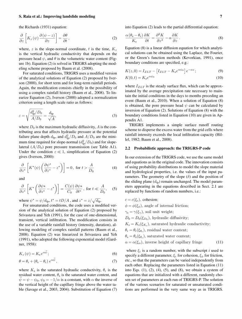
Fig. 6. The results of simulations for the Mukilteo study area, pre-sented using ROC curves. The grey square and circle represent theresults obtained using the original TRIGRS code with saturated andunsaturated initial conditions, respectively (Figure 3b, c); the curvescorrespond to the results obtained with the TRIGRS-P code, usingthe variability of input parameters shown in the inset as describedin the text (Figures 4 and 5).
The depth to the potential sliding plane dfp was assumed tocoincide with the soil depth, and was estimated by Godt et al.(2008) and Baum et al. (2010) using variations of the modelsproposed by DeRose (1996) and by Salciarini et al. (2006).Additional choices for initial conditions and correspondingsources of uncertainties will be discussed in the following.
We have implemented two probability density functions(pdf) for generating the modeling parameters: (i) the nor-mal distribution functionN , and (ii) the uniform distributionfunction U . If ξ is a standard normally distributed variableN (0,1) with mean ξ = 0 and standard deviation σ = 1, thevariable x= x+σxξ is normally distributed with mean x andstandard deviation σx, N (x,σx). Similarly, if ξ is standarduniformly distributed U(0,1), the variable y = ya+(yb−ya)ξ
Table 1. Geotechnical parameters for the geological units croppingout in the Mukilteo area (Figure 3a). c, cohesion; D0, hydraulicdiffusivity;Ks, saturated hydraulic conductivity; θs, saturated watercontent; θr, residual water content; α, inverse of capillary fringe.The friction angle φ has a common value of 33.6◦ for the threegeological units; units definitions are: 1, Qtb; 2, Qva; 3, Qvt.
Unit c D0 Ks θs θr α[kPa] [m2 s−1] [m s−1] – – [m−1]
1 3.0 3.8 · 10−4 1.0 · 10−4 0.40 0.06 102 3.0 5.0 · 10−6 1.0 · 10−7 0.40 0.10 23 8.0 8.3 · 10−6 1.0 · 10−6 0.45 0.10 5
285000 290000
4755
000
4745
000
295000
285000 290000 295000
4755
000
4745
000
4750
000
4750
000
0 3 km1.5
Collazzone
UMBRIA
Frontignano Study Area
CollazzonePerugia
Fig. 7. Map showing location of the Frontignano study area, Um-bria, central Italy. The area is located inside the larger Collazzonearea (Guzzetti et al., 2006a,b).
is uniformly distributed in the range [ya,yb], U(ya,yb). Theadvantage of using these expansions is that their determinis-tic limits are obtained for σx→ 0 and for λ≡ yb− ya→ 0,respectively.
In this work, we calculated the stability conditions in themodeling domain for a given set of variables describing theslope materials properties (φ, c, γs, Ks, D0, θr, θs) obtainedby sampling randomly from the uniform distribution only.There is a conceptual difference between the two distribu-tions for distributed landslide probabilistic modeling. Adop-tion of the Gaussian distribution requires that the investiga-tor has determined (e.g., through sufficient field tests or lab-oratory experiments) the uncertainty and measuring errorsassociated with the parameters. The mean and the standarddeviation of the Gaussian distribution define unambiguously
Table 2. Estimators of model performance for saturated and unsat-urated soil calculated with the original TRIGRS code, for the Muk-ilteo study area. TPR, True Positive Rate; FPR, False Positive Rate;ACC, Accuracy; PPV, Precision.
Model type TPR FPR ACC PPV
Saturated 0.71 0.38 0.63 0.17Unsaturated 0.41 0.12 0.84 0.28
S. Raia et al.: Improving landslide modeling 9
the uncertainty. Use of the uniform distribution implies thatthe investigator only knows the possible (or probable) rangeof variation of the parameters, ignoring the internal struc-ture of the uncertainty. We consider the Gaussian distribu-tion more appropriate to predict rainfall-induced landslidesin small areas where sufficient field and laboratory tests wereperformed to characterize the physical properties of the ge-ological materials, and the uniform distribution best suitedin the investigation of large areas where information on thegeo-hydrological properties is limited. Further, we consideruse of the Gaussian distribution best suited to investigate howerrors in the parameters propagate and affect the modeling re-sults, provided that the errors are known. Conversely, use ofthe uniform distribution allows for investigating how the un-certainty in the model parameters affects the model results.The sensitivity of the extended model to the random varia-tion of model parameters has been explored by running 16independent simulations, each with a different set of inputparameters while keeping unchanged, and equal to the runperformed with the original fixed-input TRIGRS model, theterrain morphology (δ) and rainfall history.
3 Deterministic vs. probabilistic approach
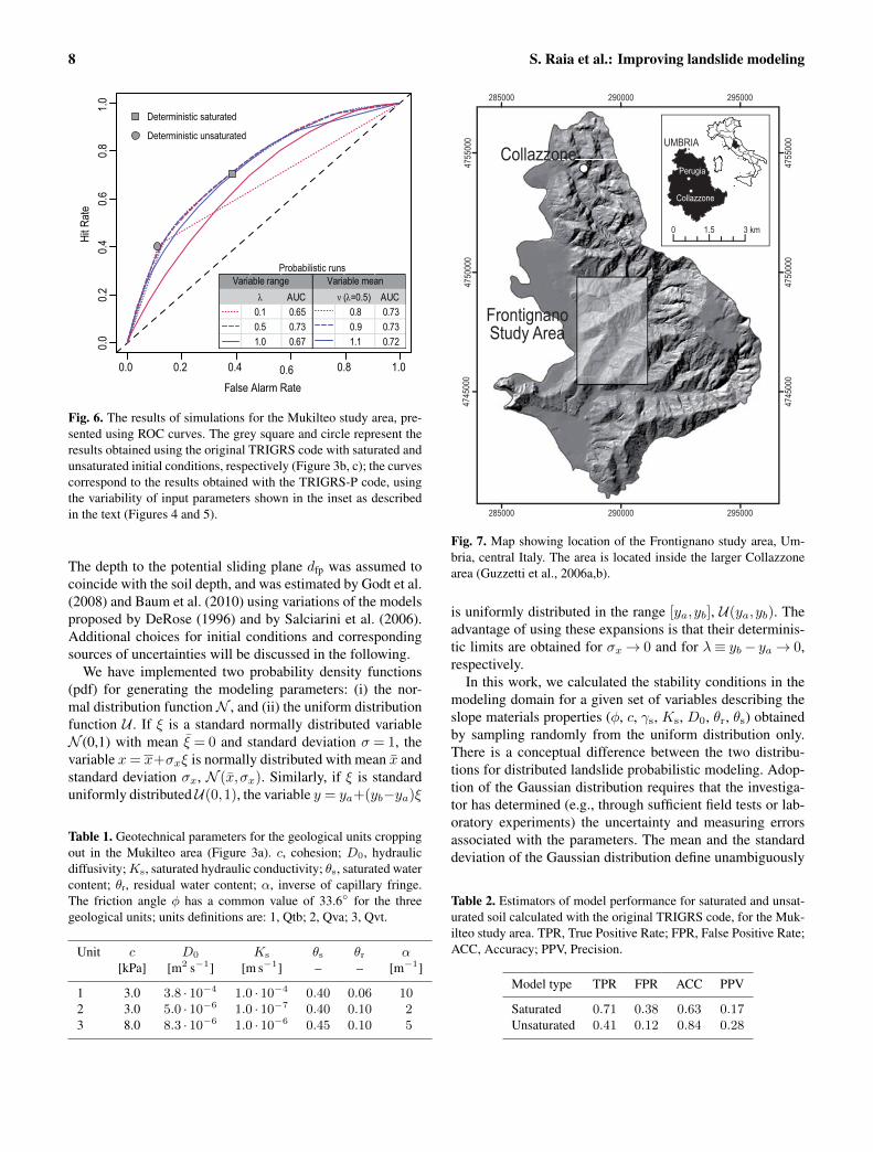
We tested the performance of the new probabilistic versionof the numerical code, TRIGRS-P 2.0, against the origi-nal TRIGRS code, version 2.0 (Baum et al., 2008), in twostudy areas. The first test was conducted in the Mukilteostudy area, near Seattle, WA, USA (Figure 2). This is thesame geographical area where Godt et al. (2008) and Baumet al. (2010) demonstrated the use of TRIGRS in a broadgeographical setting. The second test was performed in theFrontignano study area, Perugia, Italy (Figure 7). This is partof the Collazzone geographical area where Guzzetti et al.(2006a,b) have investigated the hazard posed by shallowlandslides using multivariate classification methods.
3.1 Mukilteo study area
The three square kilometre study area is located along theeastern side of the Puget Sound, about 15km north of Seattle,WA, USA (Figure 2). In this area, rainfall is the primary trig-ger of landslides. Slope failures are typically shallow (lessthan three meters thick), and involve the sandy colluviumand the weathered glacial deposits mantling the coastal bluffs(Galster and Laprade, 1991; Baum et al., 2000). The cli-mate of the Seattle area is characterized by a pronouncedseasonal precipitation regime with a winter maximum, and3/4 of the annual precipitation falling from November toApril (Church, 1974). Storms that trigger shallow landslidesin Seattle are generally of long duration (more than 24 h) andof moderate intensity (Godt et al., 2006). Three geologicalunits crop out in the area (Minard, 2000) (Figure 3a) includ-ing, from older to younger: (i) transition sediments, compris-
ing the Lawton Clay (Qtb), (ii) advance outwash sand (Qva),and (iii) glacial till (Qvt). The mechanical and hydrologicalproperties of the materials in the three geological units areknown through field tests and laboratory experiments (Luet al., 2006; Godt et al., 2006, 2008), and are summarizedin Table 1.
3.1.1 Predictions with the deterministic approach
For modeling purposes, the topography of the area wasdescribed by a 6ft× 6ft (1.83m× 1.83m) DEM obtainedthrough airborne laser-swath mapping (Haugerud et al.,2003). Initial conditions for infiltration were prescribed aszero pressure head at the depth of the lower boundary of col-luvium. This is in agreement with field observations (Baumet al., 2005; Schulz, 2007; Godt et al., 2008). A constantrainfall intensity I = 4.5mmh−1 for a period of 28 h wasused to force slope instability, for a cumulative event rainfallE = 126mm. The adopted rainfall history represents a limitcase of the rainfall intensity-duration conditions that have re-sulted in landslides in the Mukilteo area in the winter 1996–1997 (Godt et al., 2008; Baum et al., 2010). Figure 3 showsthe results of the runs with deterministic input, for saturated(Equation 4, Figure 3b) and for unsaturated (Equation 5,Figure 3c) conditions. For the mechanical and hydrologicalproperties of the geological materials (φ, c, γs, Ks, D0, θr,θs) we considered the values listed in Table 1.
In order to test the model prediction skills i.e., the abilityof the model to forecast the known distribution of rainfall-induced landslides (Guzzetti et al., 2006a), the two geograph-ical distributions of the factor of safety FS were comparedto a landslide inventory showing slope failures triggered byrainfall in the winter 1996–1997 (Baum et al., 2000; Godtet al., 2008), displayed by black lines in Figure 3. For thecomparison, all grid cells with FS < 1 were considered un-stable (i.e., potential landslide) cells. Four-fold plots andmaps showing the geographical distribution of the correctassignments and the model errors (Figure 3e, f) are used tosummarize and display the comparison. Four-fold plots aregraphical representations of contingency tables (or confusionmatrices), and show the fraction (or number) of true posi-tives (TP), true negatives (TN), false positives (FP), and falsenegatives (FN) (Fawcett, 2006; Rossi et al., 2010). In ouranalysis TP is the percentage of cells with observed land-slides, which are predicted as unstable by the model; simi-larly, TN is the percentage of cells without landslides pre-dicted as stable by the model. Correspondingly, FP (FN) arethe percentage of predicted unstable (stable) cells without(with) observed landslides. We will refer to both TP and TNas correct assignment in the following, while FP and FN aremodel errors. To further quantify the performance of the de-terministic forecasts, different metrics were computed (Ta-ble 2), including the True Positive Rate (sensitivity, or hitrate) TPR = TP/(TP + FN), the True Negative Rate (speci-ficity) TNR = TN/(FP + TN), the False Positive Rate (1 –
10 S. Raia et al.: Improving landslide modeling
288500 289500
4748
500
4749
500
4745
500
4746
500
4747
500
4748
000
4749
000
4746
000
4747
000
290500
289000 290000 291000
288500 289500
4748
500
4749
500
4745
500
4746
500
4747
500
4748
000
4749
000
4746
000
4747
000
290500
289000 290000 291000
288500 289500
4748
500
4749
500
4745
500
4746
500
4747
500
4748
000
4749
000
4746
000
4747
000
290500
289000 290000 291000
Factor of safety, Fs0.7 0.9 1.1 1.3 1.5
0° 90°Slope, δ
flyschsd cl gr-sd-st-cl sd-st-clLithology
A B C
288500 289500
4748
500
4749
500
4745
500
4746
500
4747
500
4748
000
4749
000
4746
000
4747
000
290500
289000 290000 291000
D
288500 289500
4748
500
4749
500
4745
500
4746
500
4747
500
4748
000
4749
000
4746
000
4747
000
289000 290000 291000
290500
E
289500
4748
500
4749
500
4745
500
4746
500
4747
500
4748
000
4749
000
4746
000
4747
000
290500
289000 290000 291000
288500
F74.1
0.9
24.4
0.6
TPFPTN
FN
85.8
1.2
12.7
0.3TP
FPTN
FN
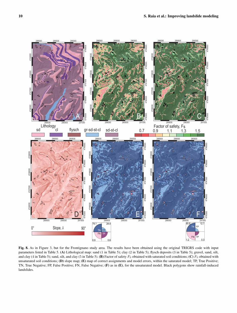
Fig. 8. As in Figure 3, but for the Frontignano study area. The results have been obtained using the original TRIGRS code with inputparameters listed in Table 5. (A) Lithological map: sand (1 in Table 5); clay (2 in Table 5); flysch deposits (3 in Table 5); gravel, sand, silt,and clay (4 in Table 5); sand, silt, and clay (5 in Table 5). (B) Factor of safety FS obtained with saturated soil conditions; (C) FS obtained withunsaturated soil conditions; (D) slope map; (E) map of correct assignments and model errors, within the saturated model; TP, True Positive;TN, True Negative; FP, False Positive; FN, False Negative; (F) as in (E), for the unsaturated model. Black polygons show rainfall-inducedlandslides.
S. Raia et al.: Improving landslide modeling 11
288500 289500
4748
500
4749
500
4745
500
4746
500
4747
500
4748
000
4749
000
4746
000
4747
000
290500
289000 290000 291000
288500 289500
4748
500
4749
500
4745
500
4746
500
4747
500
4748
000
4749
000
4746
000
4747
000
290500
289000 290000 291000
288500 28950047
4850
047
4950
047
4550
047
4650
047
4750
0
4748
000
4749
000
4746
000
4747
000
289000 290000 291000
290500 289500
4748
500
4749
500
4745
500
4746
500
4747
500
4748
000
4749
000
4746
000
4747
000
290500
289000 290000 291000
288500
288500 289500
4748
500
4749
500
4745
500
4746
500
4747
500
4748
000
4749
000
4746
000
4747
000
290500
289000 290000 291000
288500 289500
4748
500
4749
500
4745
500
4746
500
4747
500
4748
000
4749
000
4746
000
4747
000
290500
289000 290000 291000
Factor of safety, Fs0.7 0.8 0.9 1.0 1.1 1.2 1.3 1.4 1.5
A B C
D E F
ν=0.8 ν=1.1
λ=0.01 λ=0.75 λ=1.0
ν=0.9
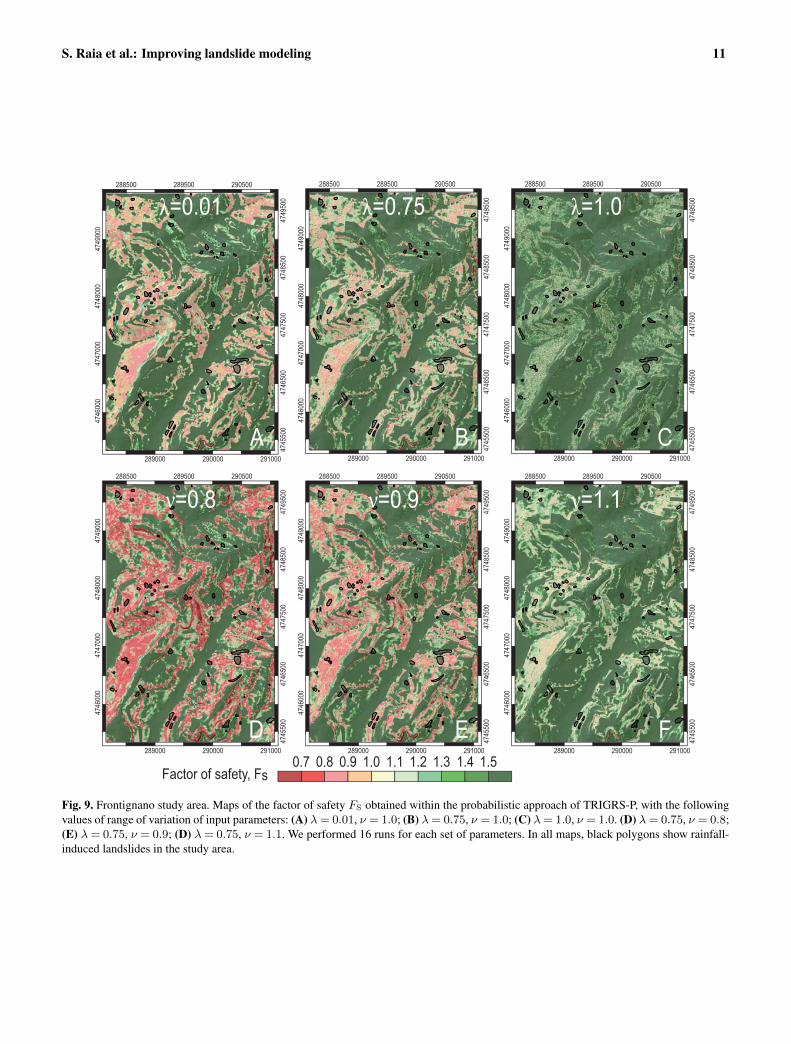
Fig. 9. Frontignano study area. Maps of the factor of safety FS obtained within the probabilistic approach of TRIGRS-P, with the followingvalues of range of variation of input parameters: (A) λ= 0.01, ν = 1.0; (B) λ= 0.75, ν = 1.0; (C) λ= 1.0, ν = 1.0. (D) λ= 0.75, ν = 0.8;(E) λ= 0.75, ν = 0.9; (D) λ= 0.75, ν = 1.1. We performed 16 runs for each set of parameters. In all maps, black polygons show rainfall-induced landslides in the study area.
12 S. Raia et al.: Improving landslide modeling
288500 289500
4748
500
4749
500
4745
500
4746
500
4747
500
4748
000
4749
000
4746
000
4747
000
290500
289000 290000 291000
288500 289500
4748
500
4749
500
4745
500
4746
500
4747
500
4748
000
4749
000
4746
000
4747
000
290500
289000 290000 291000
288500 289500
4748
500
4749
500
4745
500
4746
500
4747
500
4748
000
4749
000
4746
000
4747
000
289000 290000 291000
290500 289500
4748
500
4749
500
4745
500
4746
500
4747
500
4748
000
4749
000
4746
000
4747
000
290500
289000 290000 291000
288500
288500 289500
4748
500
4749
500
4745
500
4746
500
4747
500
4748
000
4749
000
4746
000
4747
000
290500
289000 290000 291000
288500 289500
4748
500
4749
500
4745
500
4746
500
4747
500
4748
000
4749
000
4746
000
4747
000
290500
289000 290000 291000
A B C
D E F
ν=0.8 ν=1.1
λ=0.01 λ=0.75 λ=1.0
ν=0.9
74.5
0.8
27.0
0.7
TPFPTN
FN
82.2
1.1
16.3
0.4
TPFPTN
FN
94.9
1.4
3.6
0.1
TP
FPTN
FN
74.1
0.9
24.4
0.6
TPFPTN
FN
62.5
0.7
36.0
0.8
TPFPTN
FN
92.1
1.3
6.4
0.2
FPTN
FN TP
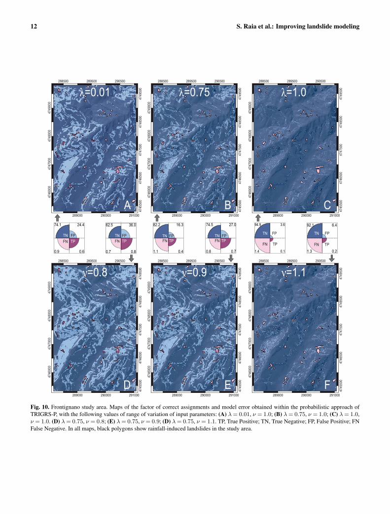
Fig. 10. Frontignano study area. Maps of the factor of correct assignments and model error obtained within the probabilistic approach ofTRIGRS-P, with the following values of range of variation of input parameters: (A) λ= 0.01, ν = 1.0; (B) λ= 0.75, ν = 1.0; (C) λ= 1.0,ν = 1.0. (D) λ= 0.75, ν = 0.8; (E) λ= 0.75, ν = 0.9; (D) λ= 0.75, ν = 1.1. TP, True Positive; TN, True Negative; FP, False Positive; FNFalse Negative. In all maps, black polygons show rainfall-induced landslides in the study area.
S. Raia et al.: Improving landslide modeling 13
0.0 0.2 0.4 0.6 0.8 1.0
0.0
0.2
0.4
0.6
0.8
1.0
False Alarm Rate
Hit R
ate
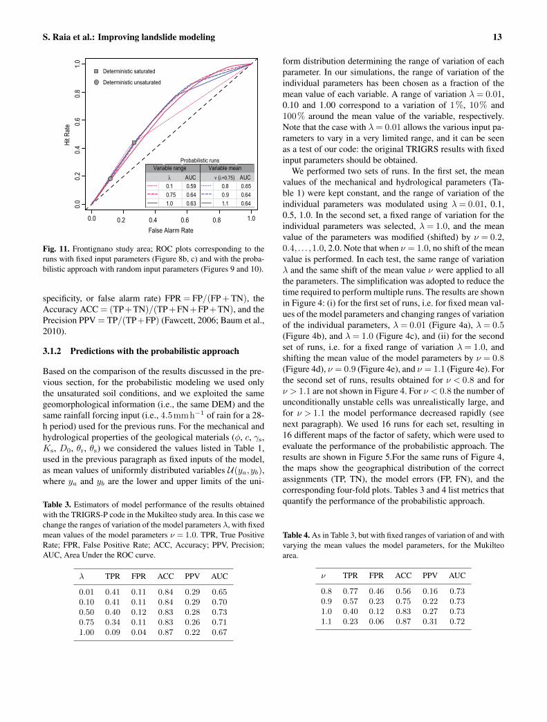
AUC AUC0.1 0.59 0.8 0.650.75 0.64 0.9 0.641.0 0.63 1.1 0.64
Variable range Variable meanν (λ=0.75)λ
Probabilistic runs
Deterministic unsaturated
Deterministic saturated
Fig. 11. Frontignano study area; ROC plots corresponding to theruns with fixed input parameters (Figure 8b, c) and with the proba-bilistic approach with random input parameters (Figures 9 and 10).
specificity, or false alarm rate) FPR = FP/(FP + TN), theAccuracy ACC = (TP+TN)/(TP+FN+FP+TN), and thePrecision PPV = TP/(TP+FP) (Fawcett, 2006; Baum et al.,2010).
3.1.2 Predictions with the probabilistic approach
Based on the comparison of the results discussed in the pre-vious section, for the probabilistic modeling we used onlythe unsaturated soil conditions, and we exploited the samegeomorphological information (i.e., the same DEM) and thesame rainfall forcing input (i.e., 4.5mmh−1 of rain for a 28-h period) used for the previous runs. For the mechanical andhydrological properties of the geological materials (φ, c, γs,Ks, D0, θr, θs) we considered the values listed in Table 1,used in the previous paragraph as fixed inputs of the model,as mean values of uniformly distributed variables U(ya,yb),where ya and yb are the lower and upper limits of the uni-
Table 3. Estimators of model performance of the results obtainedwith the TRIGRS-P code in the Mukilteo study area. In this case wechange the ranges of variation of the model parameters λ, with fixedmean values of the model parameters ν = 1.0. TPR, True PositiveRate; FPR, False Positive Rate; ACC, Accuracy; PPV, Precision;AUC, Area Under the ROC curve.
λ TPR FPR ACC PPV AUC
0.01 0.41 0.11 0.84 0.29 0.650.10 0.41 0.11 0.84 0.29 0.700.50 0.40 0.12 0.83 0.28 0.730.75 0.34 0.11 0.83 0.26 0.711.00 0.09 0.04 0.87 0.22 0.67
form distribution determining the range of variation of eachparameter. In our simulations, the range of variation of theindividual parameters has been chosen as a fraction of themean value of each variable. A range of variation λ= 0.01,0.10 and 1.00 correspond to a variation of 1%, 10% and100% around the mean value of the variable, respectively.Note that the case with λ= 0.01 allows the various input pa-rameters to vary in a very limited range, and it can be seenas a test of our code: the original TRIGRS results with fixedinput parameters should be obtained.
We performed two sets of runs. In the first set, the meanvalues of the mechanical and hydrological parameters (Ta-ble 1) were kept constant, and the range of variation of theindividual parameters was modulated using λ= 0.01, 0.1,0.5, 1.0. In the second set, a fixed range of variation for theindividual parameters was selected, λ= 1.0, and the meanvalue of the parameters was modified (shifted) by ν = 0.2,0.4, . . . ,1.0, 2.0. Note that when ν = 1.0, no shift of the meanvalue is performed. In each test, the same range of variationλ and the same shift of the mean value ν were applied to allthe parameters. The simplification was adopted to reduce thetime required to perform multiple runs. The results are shownin Figure 4: (i) for the first set of runs, i.e. for fixed mean val-ues of the model parameters and changing ranges of variationof the individual parameters, λ= 0.01 (Figure 4a), λ= 0.5(Figure 4b), and λ= 1.0 (Figure 4c), and (ii) for the secondset of runs, i.e. for a fixed range of variation λ= 1.0, andshifting the mean value of the model parameters by ν = 0.8(Figure 4d), ν = 0.9 (Figure 4e), and ν = 1.1 (Figure 4e). Forthe second set of runs, results obtained for ν < 0.8 and forν > 1.1 are not shown in Figure 4. For ν < 0.8 the number ofunconditionally unstable cells was unrealistically large, andfor ν > 1.1 the model performance decreased rapidly (seenext paragraph). We used 16 runs for each set, resulting in16 different maps of the factor of safety, which were used toevaluate the performance of the probabilistic approach. Theresults are shown in Figure 5.For the same runs of Figure 4,the maps show the geographical distribution of the correctassignments (TP, TN), the model errors (FP, FN), and thecorresponding four-fold plots. Tables 3 and 4 list metrics thatquantify the performance of the probabilistic approach.
Table 4. As in Table 3, but with fixed ranges of variation of and withvarying the mean values the model parameters, for the Mukilteoarea.
ν TPR FPR ACC PPV AUC
0.8 0.77 0.46 0.56 0.16 0.730.9 0.57 0.23 0.75 0.22 0.731.0 0.40 0.12 0.83 0.27 0.731.1 0.23 0.06 0.87 0.31 0.72
14 S. Raia et al.: Improving landslide modeling
1278000 1280000
3440
0034
6000
3400
0034
2000
3430
0034
5000
3390
0034
1000
1277000 1279000
B
1278000 1280000
3430
0034
5000
3390
0034
1000
3430
0034
5000
3390
0034
1000
1277000 1279000
C
1278000 1280000
3440
0034
6000
3400
0034
2000
3430
0034
5000
3390
0034
1000
1277000 1279000
A
Factor of safety, Fs
288500 289500
4748
500
4749
500
4745
500
4746
500
4747
500
4748
000
4749
000
4746
000
4747
000
290500
289000 290000 291000
288500 289500
4748
500
4749
500
4745
500
4746
500
4747
500
4748
000
4749
000
4746
000
4747
000
290500
289000 290000 291000
288500 289500
4748
500
4749
500
4745
500
4746
500
4747
500
4748
000
4749
000
4746
000
4747
000
290500
289000 290000 291000
A B C
λ=0.01 λ=0.5 λ=1.0
Std. dev.0.50 0.75 1.000.25
A
E
B C
D F0.7 0.8 0.9 1.0 1.1 1.2 1.3 1.51.4
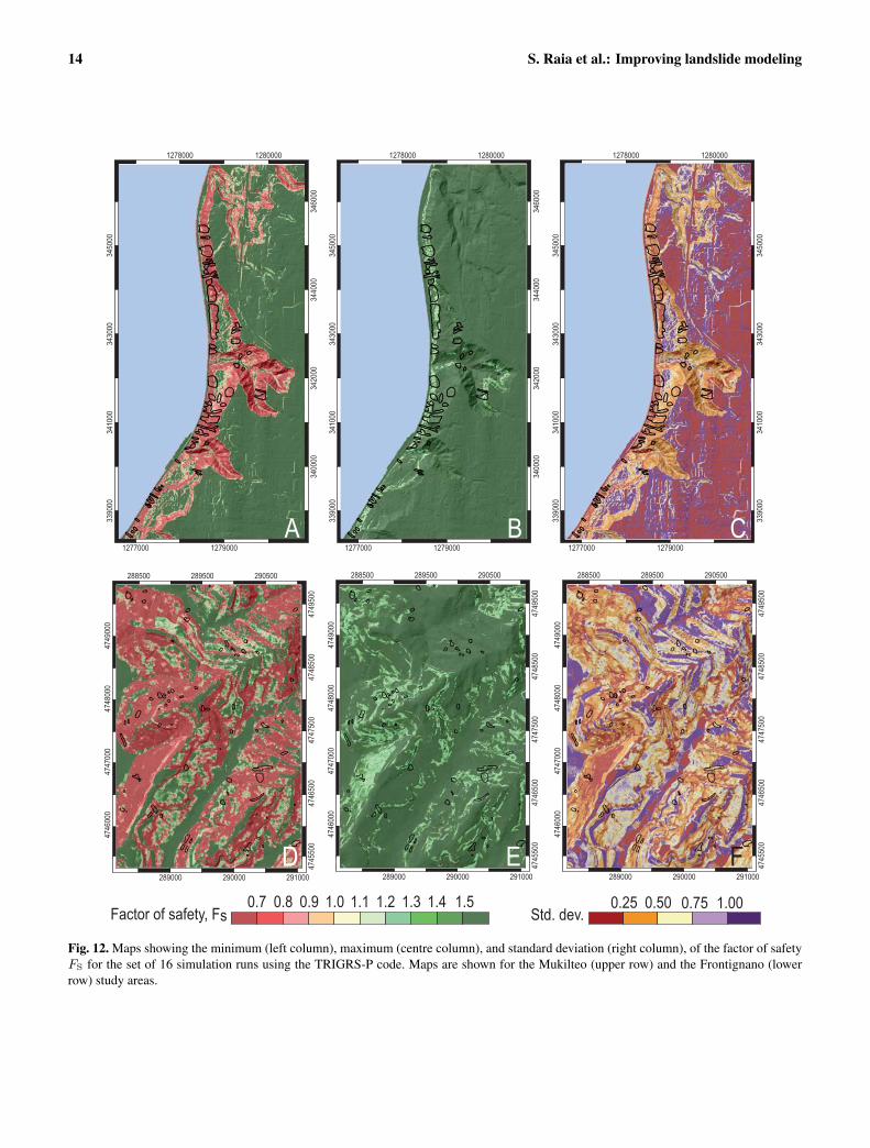
Fig. 12. Maps showing the minimum (left column), maximum (centre column), and standard deviation (right column), of the factor of safetyFS for the set of 16 simulation runs using the TRIGRS-P code. Maps are shown for the Mukilteo (upper row) and the Frontignano (lowerrow) study areas.
S. Raia et al.: Improving landslide modeling 15
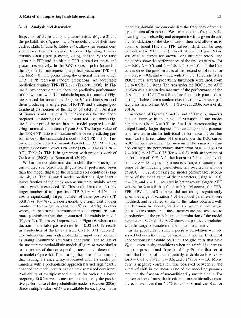
3.1.3 Analysis and discussion
Inspection of the results of the deterministic (Figure 3) andthe probabilistic (Figures 4 and 5) models, and of their fore-casting skills (Figure 6, Tables 2–4), allows for general con-siderations. Figure 6 shows a Receiver Operating Charac-teristics (ROC) plot (Fawcett, 2006), defined by the falsealarm rate FPR and the hit rate TPR, plotted on the x- andy-axes, respectively. In the ROC space, a point located inthe upper left corner represents a perfect prediction (TPR = 1and FPR = 0), and points along the diagonal line for whichTPR = FPR represent random predictions. An acceptableprediction requires TPR/FPR> 1 (Fawcett, 2006). In Fig-ure 6, two separate points show the predictive performanceof the two runs with deterministic inputs, for saturated (Fig-ure 3b) and for unsaturated (Figure 3c) conditions each ofthem producing a single pair FPR-TPR and a unique geo-graphical distribution of the factor of safety FS. Analysisof Figures 3 and 6, and of Table 2 indicates that the modelprepared considering the soil unsaturated conditions (Fig-ure 3c) performed better than the model prepared consid-ering saturated conditions (Figure 3b). The larger value ofthe TPR/FPR ratio is a measure of the better predicting per-formance of the unsaturated model (TPR/FPR = 3.46, Fig-ure 6), compared to the saturated model (TPR/FPR = 1.87,Figure 3), despite a lower TPR value (TPR = 0.42 vs. TPR =0.71, Table 2). This is in agreement with previous work ofGodt et al. (2008) and Baum et al. (2010).
Within the two deterministic models, the one using theunsaturated soil conditions (Figure 3c, f) performed betterthan the model that used the saturated soil conditions (Fig-ure 3b, e). The saturated model predicted a significantlylarger fraction of the study area as unstable, mainly whereterrain gradient exceeded 15◦. This resulted in a considerablylarger number of true positives (TP, 7.1 % vs. 4.1 %), butalso a significantly larger number of false positives (FP,33.8 % vs. 10.4 %) and a correspondingly significantly lowernumber of true negatives (TN, 56.1 % vs. 79.5 %). In otherwords, the saturated deterministic model (Figure 3b) wasmore pessimistic than the unsaturated deterministic model(Figure 3c). This is well represented in Figure 6, where a re-duction of the false positive rate from 0.38 to 0.12 resultsin a reduction of the hit rate from 0.71 to 0.41 (Table 2).The subsequent runs with probabilistic input were obtainedassuming unsaturated soil water conditions. The results ofthe unsaturated probabilistic models (Figure 4) were similarto the results of the corresponding unsaturated determinis-tic model (Figure 3c). This is a significant result, confirmingthat treating the uncertainty associated with the model pa-rameters with a probabilistic approach has not significantlychanged the model results, which have remained consistent.Availability of multiple model outputs for each run allowedpreparing ROC curves to measure quantitatively the predic-tive performance of the probabilistic models (Fawcett, 2006).Since multiple values of FS are available for each pixel in the
modeling domain, we can calculate the frequency of stabil-ity condition of each pixel. We attribute to this frequency themeaning of a probability and compare it with a given thresh-old. Modulation of the classification threshold allows us toobtain different FPR and TPR values, which can be usedto construct a ROC curve (Fawcett, 2006). In Figure 6 twosets of ROC curves are shown using different colors. Thered curves show the performances of the first set of runs, forλ= 0.01, λ= 0.5, and λ= 1.0, with ν = 1.0, and the bluecurves show the performances of the second set of runs, forν = 0.8, ν = 0.9, and ν = 1.1, with λ= 0.5. To construct theROC curves, several probability thresholds were used, from0.1 to 0.9 by 0.1 steps. The area under the ROC curve AUCis taken as a quantitative measure of the performance of theclassification. If AUC = 0.5, a classification is poor and in-distinguishable from a random classification, whereas a per-fect classification has AUC = 1 (Fawcett, 2006; Rossi et al.,2010).
Inspection of Figures 5 and 6, and of Table 3, suggeststhat an increase in the range of variation of the modelparameters (from λ= 0.01 to λ= 1.0), corresponding toa significantly larger degree of uncertainty in the parame-ters, resulted in similar individual performance indices, butsignificantly larger values of the area under the ROC curve,AUC. In our experiment, the increase in the range of varia-tion changed the performance index from AUC = 0.65 (forλ= 0.01) to AUC = 0.73 (for λ= 0.5), with an increase ofperformance of 16 %. A further increase of the range of vari-ation to λ= 1.0, a possibly unrealistic range of variation forsome of the modeling parameters, has resulted in a valueof AUC = 0.67, decreasing the model performance. Modu-lation of the mean value of the parameters, using ν = 0.8,ν = 0.9, and ν = 1.1, resulted in better results (larger AUCvalues) for λ= 0.5 than for λ= 0.01. Moreover, the TPR,FPR, PPV and ACC metrics did not change significantlywhen the range of variation λ of the model parameters weremodified, and remained similar to the values obtained withthe deterministic models, for λ≤ 0.5. We conclude that, inthe Mukilteo study area, these metrics are not sensitive tointroduction of the probabilistic determination of the modelparameters. Second, the AUC showed a positive correlationwith the range of variation in the model parameters.
In the probabilistic runs, a positive correlation was ob-served between the range of variation λ and the fraction ofunconditionally unstable cells i.e., the grid cells that haveFS < 1 even in dry conditions when no rainfall is increas-ing pore pressure and slope instability. For the first set ofruns, the fraction of unconditionally unstable cells was 0%for λ= 0.01, 0.3% for λ= 0.5, and 0.7% for λ= 1.0. More-over, a negative correlation was observed between ν, thewidth of shift in the mean value of the modeling parame-ters, and the fraction of unconditionally unstable cells. Forthe second set of runs, the fraction of unconditionally unsta-ble cells was less than 5.0% for ν ≥ 0.8, and was 0% for
16 S. Raia et al.: Improving landslide modeling
ν > 1.0, independent of the range of variation of the param-eters.
3.2 Frontignano study area
The Frontignano area is located in central Umbria, Italy,about 25km south of Perugia, in the Collazzone area (Fig-ure 7). In this area, landslides are caused primarily by rainfalland rapid snowmelt (Cardinali et al., 2000; Guzzetti et al.,2006a,b; Fiorucci et al., 2011). Multiple deep-seated andshallow slides were identified in the area through the visualinterpretation of multiple sets of aerial photographs and very-high resolution satellite images, and field surveys.
The shallow failures are typically less than three metersthick, and involve the soil and the colluvium mantling theslopes. Soils range in thickness from a few decimetres tomore than one meter; they have a fine to medium texture, andexhibit a xeric moisture regime, typical of the Mediterraneanclimate. In central Umbria, precipitation is most abundant inOctober and November, with a mean annual rainfall in theperiod 1921–2001 exceeding 850 mm. In the study area, ter-rain is hilly, and the lithology and the attitude of beddingplanes control the morphology of the slopes. Gravel, sand,clay, travertine, layered sandstone and marl, and thinly lay-ered limestone, crop out in the area (Cardinali et al., 2000;Guzzetti et al., 2006a,b).
3.2.1 Predictions with the deterministic approach
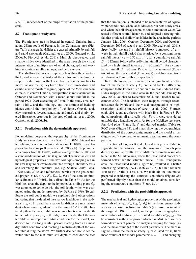
For modeling purposes, the topography of the Frontignanostudy area was described by a 5m× 5m DEM obtained in-terpolating 5-m contour lines shown on 1 : 10000 scale to-pographic base maps (Guzzetti et al., 2006a,b). Slope in thearea ranges from 0◦ to 62◦, with an average value of 10◦ anda standard deviation of 5.6◦ (Figure 8d). The mechanical andhydrological properties of the five soil types cropping out inthe area (Figure 8a) were determined through laboratory testsand searching the literature (see, e.g. Shafiee, 2008; Feda,1995; Lade, 2010, and references therein) on the geotechni-cal properties (φ, c, γs, Ks, D0, θr, θs) of the same or simi-lar sediments in Umbria, Italy (listed in Table 5). As for theMukilteo area, the depth to the hypothetical sliding plane dfpwas assumed to coincide with the soil depth, which was esti-mated using the model proposed by DeRose (1996). To cal-ibrate the soil depth model, we exploited field observationsindicating that the depth of the shallow landslides in the studyarea is dfp < 3 m, and that shallow landslides are most abun-dant where terrain gradient is in the range 7◦ ≤ δ ≤ 20◦. Ini-tial depth to the water table was set to a fraction of the depthto the failure plane, dw = 0.85dfp. Since the depth of the wa-ter table is an important initial condition for the model, wedecided to use a long rainfall period, starting from an almostdry initial condition and reaching a realistic depth of the wa-ter table during the storm. We further decided not to set thewater table to the maximum soil depth to consider the fact
that the simulation is intended to be representative of typicalwinter conditions, when landslides occur in both study areas,and when the soil always contains some amount of water. Wetested different rainfall histories, and adopted a forcing rain-fall that produced shallow landslides in the area in the periodsJanuary–May 2004, October–December 2004, and October–December 2005 (Guzzetti et al., 2009; Fiorucci et al., 2011).Specifically, we used a rainfall history composed of a 4-week initial rainfall period characterized by a constant meanrainfall intensity I = 0.36mmh−1, for a cumulative rainfallE = 242mm, followed by a 60-min rainfall period character-ized by a high rainfall intensity I = 90mmh−1, for a cumu-lative rainfall E = 90mm. Results for the saturated (Equa-tion 4) and the unsaturated (Equation 5) modeling conditionsare shown in Figures 8b, c, respectively.
To test the model performance, the geographical distribu-tion of the factor of safety FS predicted by TRIGRS werecompared to the known distribution of rainfall-induced land-slides mapped in the same area in the periods January toMay 2004, October to December 2004, and October to De-cember 2005. The landslides were mapped through recon-naissance fieldwork and the visual interpretation of high-resolution satellite images (Guzzetti et al., 2009; Fiorucciet al., 2011), and are shown with black lines in Figure 8. Forthe comparison, all grid cells with FS < 1 were consideredunstable (i.e., landslide) cells. As for the Mukilteo test case,four-fold plots (Figure 8e, f) and derived metrics (Table 6),ROC plots (Figure 11), and maps showing the geographicaldistribution of the correct assignments and the model errors(Figure 8e, f) were used to summarize and measure the com-parison.
Inspection of Figures 8 and 11, and analysis of Table 6,suggests that the saturated and the unsaturated models pro-duce very similar results. This is different from the result ob-tained in the Mukilteo area, where the unsaturated model per-formed better than the saturated model. In the Frontignanoarea, the unsaturated model (Figure 8c) resulted in a betterforecasting accuracy (ACC, 0.86 vs. 0.75), but in a reducedTPR to FPR ratio (1.4 vs. 1.7). We maintain that the modelprepared considering the saturated conditions (Figure 8b)performed slightly better than the model obtained consider-ing the unsaturated conditions (Figure 8c).
3.2.2 Predictions with the probabilistic approach
The mechanical and hydrological properties of the geologicalmaterials (φ, c, γs, Ks, D0, θr, θs) in the Frontignano studyarea were chosen as listed in Table 5 (also used as input ofthe original TRIGRS model, in the previous paragraph) asmean values of uniformly distributed variables U(ya,yb). Tobe consistent with the approach adopted in Mukilteo, we per-formed two sets of parametric analyses, varying the range (λ)and the mean value (ν) of the model parameters. The maps inFigure 9 show the factor of safety FS calculated for: (i) fixedmean values of the model parameters ν = 1.0, and changing
S. Raia et al.: Improving landslide modeling 17C
ount
050
010
0015
0020
0025
00C
ount
050
010
0015
0020
00
Factor of safety, Fs
Cou
nt
0 2 4 6 8 10
050
010
0015
0020
00
0 1 2 3 4 5 6 7 8 9 10
Cou
nt0
500
1000
1500
2000
2500
Cou
nt0
500
1000
1500
2000
Factor of safety, Fs
Cou
nt
0 2 4 6 8 10
050
010
0015
0020
00
0 1 2 3 4 5 6 7 8 9 10
A
C
B
D
E
F
Fig. 13. Histograms showing the distribution of the values of theFS for the Mukilteo (left, A, B, C) and the Frontignano (right, D,E, F) study areas. (A) and (D) for subsets of 1000 grid cells with0< F S ≤ 1.5. (B) and (E) for subsets of 1000 grid cells with 1.5<F S ≤ 3. (C) and (F) for subsets of 1000 grid cells with such thatF S > 3.
ranges of variation of the individual parameters, λ= 0.01(Figure 9a), λ= 0.75 (Figure 9b), and λ= 1.0 (Figure 9c),and (ii) a fixed range of variation λ= 0.75, and shifting themean value of the model parameters by ν = 0.8 (Figure 9d),ν = 0.9 (Figure 9e), and ν = 1.1 (Figure 9f). As in the previ-ous case, λ= 0.01 corresponds to a very small range of vari-ability of the parameters, and provides the same results. Forν = 1.0, no shift in the mean values of the model parametersis performed. The degree of accuracy of the two sets of runsfor the Frontignano area is shown in Figure 10, for the samemodels shown in Figure 9. The maps show the geographicaldistribution of the correct assignments (TP, TN), the modelerrors (FP, FN), and the corresponding four-fold plots. Ta-bles 7 and 8 list metrics that quantify the performance of theruns. The performance of the probabilistic models is furtheranalysed in Figure 11 by two sets of ROC curves, shown us-ing different colours; red curves for the case of variable rangeλ, and blue curves for the case of a variable mean ν. In thesame plot, the grey circle shows the predicting performanceof the saturated model (Figure 8b), and the grey square the
performance of the unsaturated model (Figure 8c) both runwith fixed input parameters.
3.2.3 Analysis and discussion
Inspection of the results of the fixed input runs (Figure 8),the runs with input parameter sampled from a suitable prob-ability distribution, (Figures 9 and 10), and of their abil-ity to forecast the spatial distribution of known landslides(Figure 11, Tables 6–8), allows for considerations that aresimilar to those discussed for the Mukilteo study area (seeSect. 3.1.3), with a few differences. In the Frontignanoarea, the saturated and the unsaturated models providednearly equivalent results, with the saturated model consid-ered marginally superior primarily because of the reducedvalue of the TPR to FPR ratio. From a statistical point ofview, given the reduced fraction of landslide area in Fron-tignano (1.5%) compared to Mukilteo (4.2%), the spatialprediction of landslides in Frontignano was more difficultthan in Mukilteo. From a physical point of view, modelingthe stability conditions in low gradient terrain is very sensi-tive to the initial conditions, which are uncertain and diffi-cult to determine spatially. The runs with variable input pa-rameters confirm the slightly poorer geographical predictiveperformance of the adopted physical framework in Frontig-nano, compared to Mukilteo (Tables 3 and 4 vs. Tables 7 and8). Taking the area under the ROC curve (AUC) as the met-ric to compare the models, one can readily see that runs forthe Mukilteo area resulted in 0.65≤ AUC≤ 0.73, and forthe Frontignano area exhibited 0.59≤ AUC≤ 0.65. In otherwords, the “worst” result for Mukilteo (AUC = 0.65, for ν =1.0 and λ= 0.01) has the same overall spatial predictive per-formance of the “best” result for Frontignano (AUC = 0.65,for ν = 0.8 or 0.9 and λ= 0.75). In the Frontignano area,despite a lower “absolute” performance (i.e., when comparedto Mukilteo), adoption of a probabilistic approach improvedthe spatial forecasting skills. Again, taking AUC as a metricto compare the models, values of this metric increased fromAUC = 0.59 (for ν = 1.0 and λ= 0.01), to AUC = 0.65 (forν = 0.8 or 0.9 and λ= 0.75). This is a non-negligible im-provement of about 10%. The result confirms that adoptionof a probabilistic framework to the distributed modeling ofshallow landslides results in improved spatial forecasts.
The result further corroborates the finding that model-ing the natural uncertainty (and poor understanding) of themechanical and hydrological variables results in better spa-tial landslide predictions of the locations of rainfall-inducedlandslides (see insets in Figure 4). First, the TPR, FPR, PPV,and AUC metrics did not change significantly when the rangeof variation λ of the model parameters was changed. Thesemetrics remained similar to the values obtained with the fixedinput model, confirming that they are not sensitive to dif-ferences between probabilistic framework runs with randomvariations of parameters and runs with fixed parameters. Sec-ond, the area under the ROC curve AUC confirmed its posi-
18 S. Raia et al.: Improving landslide modeling
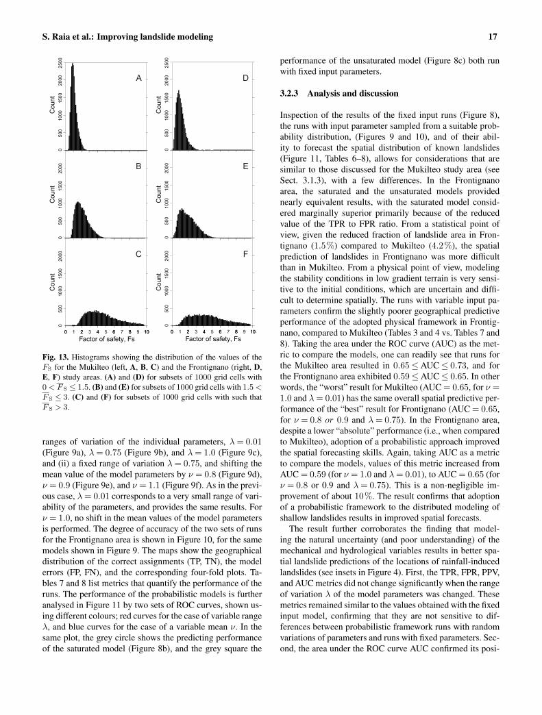
10-3
105
104
103
102
101
10-2
100
10-1
106
107
10-1
106
105
104
103
102
101
100
107108
105104103102101100
Mem
ory u
sage
[Gb
]
Area [km2]
Exec
ution
tim
e [s
]
A
TRIGRS - saturated model
1×1 m
30×30 m
10×10 m
5×5 m2×2 m
10-3
105
104
103
102
101
10-2
100
10-1
106
107
10-1
106
105
104
103
102
101
100
107
108
105104103102101100
Mem
ory u
sage
[Gb
]
Area [km2]
Exec
ution
time
[s]
B
TRIGRS-S - unsaturated model
1×1 m
30×30 m
10×10 m
5×5 m2×2 m
Fig. 14. Estimated memory usage (left y-axis) and execution times (right y-axis) for (A) the TRIGRS code (saturated model), and (B) a setof 16 runs of the TRIGRS-P code, for areas of different extent, and for grid cells of different spaptial resolutions.
tive correlation with the range of variation in the model pa-rameters λ, in support of the probabilistic approach. Third,the positive correlation between the range of variation λ andthe fraction of unconditionally unstable cells, and the neg-ative correlation between the shift in the mean value of themodeling parameters ν and the fraction of unconditionallyunstable cells, were both confirmed.
4 Discussion
Our probabilistic approach to the distributed modeling ofshallow landslides proved effective in the two study areaswhere it was tested (Figures 2 and 7). In both areas, the mapsshowing the geographical distribution of the factor of safetyFS obtained using TRIGRS-P were better predictors of thedistributions of known rainfall-induced landslides than thecorresponding maps obtained adopting the original TRIGRSapproach. This conclusion is supported by the indices usedto measure the forecasting skills of the different models, andparticularly the area under the ROC, AUC (Tables 2–4 forMukilteo, and Table 6, 7, 8 for Frontignano). The runs inwhich we allowed a large variability of the input parameters(e.g. λ= 0.50 or λ= 0.75) were better predictors of the ge-ographical distribution of known landslides than the modelsprepared using a reduced variability in the model parameters(e.g. λ= 0.1) (Guzzetti et al., 2006a; Rossi et al., 2010). Thisis shown in the insets in Figure 4, where a portion of the re-sults for the Mukilteo study area is shown at a larger scale.The variability of the geographical distribution of the FS isalso shown in Figure 12 where we have plotted the minimum,the maximum, and the standard deviation of the computed FS
values. In particular, the map of the standard deviation pro-vides quantitative and spatially distributed evidence of the
uncertainty associated with the distributed modeling of land-slide instability.
We studied the variation of the computed factor of safety.Figure 13 shows histograms for the distribution of the val-ues of the factor of safety FS in selected grid cells in theMukilteo (Figure 13a–c) and the Frontignano (Figure 13d–f)study areas. For simplicity, in the Figure we show the resultsobtained for a single lithological type i.e., the transition sed-iments (Qtb, indicated as unit 1 in Table 1) in the Mukilteoarea (Figure 3a), and the sand-silt-clay (unit 5 in Table 5)in the Frontignano area (Figure 8a). Results for other litho-logical types in the two study areas are similar. We adoptedthe following procedure to obtain the histograms. First, weperformed 100 probabilistic simulations to obtain a large setof values of the factor of safety FS, and we computed theaverage value of the factor of safety, FS for each grid cellin the two modeling domains. For both study areas, a valueof λ= 0.50 (and ν = 1.0) was used for the variability ofthe geotechnical and hydrological parameters. Next, we se-lected three subsets of 1000 grid cells, with 0< F S ≤ 1.5,1.5< F S ≤ 3.0, and F S > 3, respectively. Finally, we usedall the computed values of the FS in each subset to constructthe histograms. Inspection of the histograms reveals that forF S > 3 (Figure 13c, f) the distribution of the predicted fac-tor of safety is almost uniform and does not show a predom-inant value. Instead, for F S < 1.5 the distribution of the pre-dicted factors of safety peaks at FS ≈ 1.0 (Figure 13a, d). For1.5< F S ≤ 3.0, results are intermediate (Figure 13b, e).
In conclusion, the probabilistic approach results in a num-ber of model outputs, each representing the geographical dis-tribution of the FS values. In this work, 16 runs were per-formed. Availability of multiple results allows for the analy-sis of the sensitivity of the model to variations in the input pa-rameters controlling the stability conditions. Variability de-
S. Raia et al.: Improving landslide modeling 19
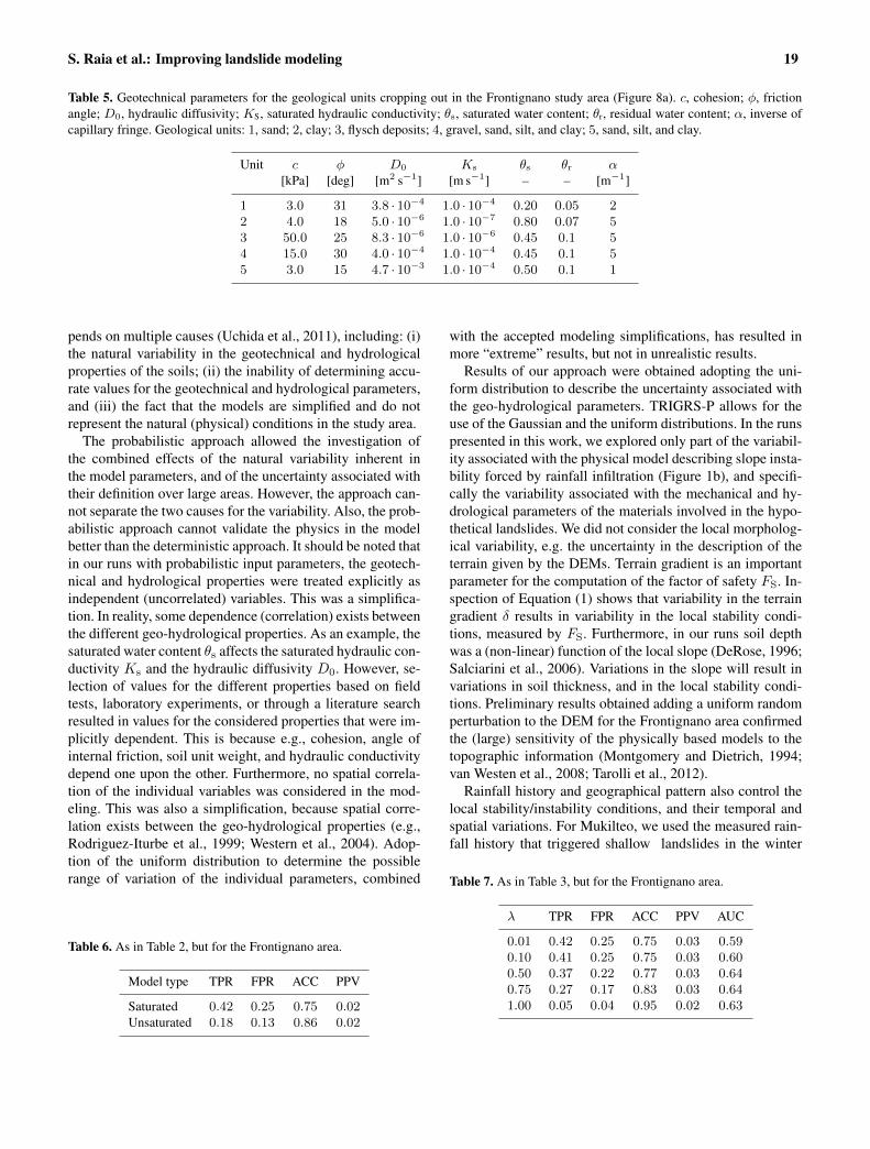
Table 5. Geotechnical parameters for the geological units cropping out in the Frontignano study area (Figure 8a). c, cohesion; φ, frictionangle; D0, hydraulic diffusivity; KS, saturated hydraulic conductivity; θs, saturated water content; θr, residual water content; α, inverse ofcapillary fringe. Geological units: 1, sand; 2, clay; 3, flysch deposits; 4, gravel, sand, silt, and clay; 5, sand, silt, and clay.
Unit c φ D0 Ks θs θr α[kPa] [deg] [m2 s−1] [m s−1] – – [m−1]
1 3.0 31 3.8 · 10−4 1.0 · 10−4 0.20 0.05 22 4.0 18 5.0 · 10−6 1.0 · 10−7 0.80 0.07 53 50.0 25 8.3 · 10−6 1.0 · 10−6 0.45 0.1 54 15.0 30 4.0 · 10−4 1.0 · 10−4 0.45 0.1 55 3.0 15 4.7 · 10−3 1.0 · 10−4 0.50 0.1 1
pends on multiple causes (Uchida et al., 2011), including: (i)the natural variability in the geotechnical and hydrologicalproperties of the soils; (ii) the inability of determining accu-rate values for the geotechnical and hydrological parameters,and (iii) the fact that the models are simplified and do notrepresent the natural (physical) conditions in the study area.
The probabilistic approach allowed the investigation ofthe combined effects of the natural variability inherent inthe model parameters, and of the uncertainty associated withtheir definition over large areas. However, the approach can-not separate the two causes for the variability. Also, the prob-abilistic approach cannot validate the physics in the modelbetter than the deterministic approach. It should be noted thatin our runs with probabilistic input parameters, the geotech-nical and hydrological properties were treated explicitly asindependent (uncorrelated) variables. This was a simplifica-tion. In reality, some dependence (correlation) exists betweenthe different geo-hydrological properties. As an example, thesaturated water content θs affects the saturated hydraulic con-ductivity Ks and the hydraulic diffusivity D0. However, se-lection of values for the different properties based on fieldtests, laboratory experiments, or through a literature searchresulted in values for the considered properties that were im-plicitly dependent. This is because e.g., cohesion, angle ofinternal friction, soil unit weight, and hydraulic conductivitydepend one upon the other. Furthermore, no spatial correla-tion of the individual variables was considered in the mod-eling. This was also a simplification, because spatial corre-lation exists between the geo-hydrological properties (e.g.,Rodriguez-Iturbe et al., 1999; Western et al., 2004). Adop-tion of the uniform distribution to determine the possiblerange of variation of the individual parameters, combined
Table 6. As in Table 2, but for the Frontignano area.
Model type TPR FPR ACC PPV
Saturated 0.42 0.25 0.75 0.02Unsaturated 0.18 0.13 0.86 0.02
with the accepted modeling simplifications, has resulted inmore “extreme” results, but not in unrealistic results.
Results of our approach were obtained adopting the uni-form distribution to describe the uncertainty associated withthe geo-hydrological parameters. TRIGRS-P allows for theuse of the Gaussian and the uniform distributions. In the runspresented in this work, we explored only part of the variabil-ity associated with the physical model describing slope insta-bility forced by rainfall infiltration (Figure 1b), and specifi-cally the variability associated with the mechanical and hy-drological parameters of the materials involved in the hypo-thetical landslides. We did not consider the local morpholog-ical variability, e.g. the uncertainty in the description of theterrain given by the DEMs. Terrain gradient is an importantparameter for the computation of the factor of safety FS. In-spection of Equation (1) shows that variability in the terraingradient δ results in variability in the local stability condi-tions, measured by FS. Furthermore, in our runs soil depthwas a (non-linear) function of the local slope (DeRose, 1996;Salciarini et al., 2006). Variations in the slope will result invariations in soil thickness, and in the local stability condi-tions. Preliminary results obtained adding a uniform randomperturbation to the DEM for the Frontignano area confirmedthe (large) sensitivity of the physically based models to thetopographic information (Montgomery and Dietrich, 1994;van Westen et al., 2008; Tarolli et al., 2012).
Rainfall history and geographical pattern also control thelocal stability/instability conditions, and their temporal andspatial variations. For Mukilteo, we used the measured rain-fall history that triggered shallow landslides in the winter
Table 7. As in Table 3, but for the Frontignano area.
λ TPR FPR ACC PPV AUC
0.01 0.42 0.25 0.75 0.03 0.590.10 0.41 0.25 0.75 0.03 0.600.50 0.37 0.22 0.77 0.03 0.640.75 0.27 0.17 0.83 0.03 0.641.00 0.05 0.04 0.95 0.02 0.63
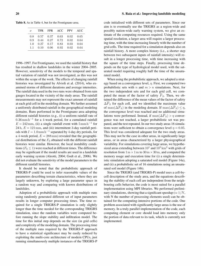
20 S. Raia et al.: Improving landslide modeling
Table 8. As in Table 4, but for the Frontignano area.
ν TPR FPR ACC PPV AUC
0.8 0.57 0.37 0.63 0.02 0.650.9 0.44 0.27 0.72 0.02 0.641.0 0.27 0.17 0.83 0.03 0.641.1 0.10 0.06 0.92 0.02 0.64
1996–1997. For Frontignano, we used the rainfall history thathas resulted in shallow landslides in the winter 2004–2005.However, sensitivity of the models to the temporal and spa-tial variation of rainfall was not investigated, as this was notwithin the scope of the work. The effects of changing rainfallhistories was investigated by Alvioli et al. (2014), who ex-amined storms of different durations and average intensities.The rainfall data used in the two runs were obtained from raingauges located in the vicinity of the study areas. The rainfallmeasurements may not represent the exact amount of rainfallat each grid cell in the modeling domain. We further assumeda uniformly distributed rainfall in the geographical modelingdomains. Runs performed in the Frontignano area adoptingdifferent rainfall histories (e.g., (i) a uniform rainfall rate of0.36mmh−1 for a 4-week period, for a cumulated rainfallE = 242mm, (ii) a single rainfall event with 5mmh−1 for24 h, E = 121mm, and (iii) intermittent 3-day rainfall peri-ods with I = 1.0mmh−1 separated by 4-day dry periods, fora 4-week period, E = 288mm) revealed that the geographi-cal distributions of the FS obtained with the different rainfallhistories were similar. However, the local instability condi-tions (FS ≤ 1) were reached at different times. The differencemay be significant if the model results are used in a landslideearly warning system (Aleotti, 2004; Godt et al., 2006). Wedid not evaluate the sensitivity of the model parameters to thedifferent rainfall histories.
It should be noted that the probabilistic approach ofTRIGRS-P could be used to infer reasonable values of theparameters describing terrain characteristics, where they arelargely unknown, by exploring a large parameter space ina random way and comparing with known distributions oflandslides.
Adoption of a probabilistic approach with multiple runsusing randomly generated different set of input parametersresults in longer computer processing times. The time re-quired for a single TRIGRS-P simulation is only slightlylonger than the time needed for the corresponding TRIGRSsimulation, since the random variables were computed be-fore running the slope stability and infiltration model. Thetime for this initial step depends on the size (in grid cells)and complexity of the modeling domain. The processing timeof the multiple runs required by the TRIGRS-P approachto have a statistical significance may be easily reduced byexploiting the multi-core architecture of modern CPUs, justrunning simultaneously multiple instances of the TRIGRS-P
code initialised with different sets of parameters. Since ouraim is to eventually use the TRIGRS as a region-wide andpossibly nation-wide early warning system, we give an es-timate of the computing resources required. Using the samespatial resolution, a larger area will require a larger process-ing time, with the time increasing linearly with the number ofgrid cells. The time required for a simulation depends also onrainfall history. A more complex history (i.e., a shorter stepbetween two subsequent inputs of rainfall intensity) will re-sult in a longer processing time, with time increasing withthe square of the time steps. Finally, processing time de-pends on the type of hydrological model used, with the sat-urated model requiring roughly half the time of the unsatu-rated model.
When using the probabilistic approach, we adopted a strat-egy based on a convergence level, η. First, we computed twoprobabilistic sets with n and m> n simulations. Next, forthe two independent sets and for each grid cell, we com-puted the mean of the factor of safety F S. Then, we ob-tained the difference of the mean values of the factor of safety∆F S for each cell, and we identified the maximum valueof max(∆F S) in the modeling domain. If max(∆F S)≤ η,the convergence level was reached and no additional simu-lations were performed. Instead, if max(∆F S)> η conver-gence was not reached, a larger probabilistic set was pre-pared, and the test repeated. In our two study areas 16 simula-tions were sufficient to obtain a convergence level η = 0.05.This level was considered adequate for the two study areas.This may not be the case in other areas, in significantly largeareas, or in areas characterized by a larger physiographicalvariability. For simulations covering large areas, we hypothe-sized areas extending between 101 and 105 km2 with grids ofresolution from 1m×1m to 30m×30m, and computed thememory usage and execution time for (i) a single determin-istic simulation adopting a saturated soil model (Figure 14a),and (ii) a probabilistic set of 16 simulations using an unsatu-rated soil model (Figure 14b).
Since the TRIGRS (and TRIGRS-P) model uses a cell-by-cell description of the study area, and the equations describ-ing the stability of each cell are independent from the neigh-bouring cells behavior, the code is most suited for a parallelimplementation using MPI libraries. We performed prelimi-nary simulations, showing that a significant speedup (' 1/N ,with N the number of processing elements used) can be ob-tained for the computing-intensive portions of the code. Oneproblem associated with significantly large areas is the use ofmemory. In a truly parallel implementation of the code, eachcomputing element or core should load into memory onlythe portion of data relevant to its task, which is currently notimplemented.
S. Raia et al.: Improving landslide modeling 21
5 Conclusions
We prepared a probabilistic version of the Transient RainfallInfiltration and Grid-Based Regional Slope-Stability Analy-sis code, TRIGRS (Baum et al., 2002, 2008), and tested thenew code TRIGRS-P in two study areas: Mukilteo, near Seat-tle, USA, and Frontignano, near Perugia, Italy. The tests sug-gest that the runs initialized with random values of the inputparameters generated according to proper probability distri-bution functions, were better predictors of the spatial locationof rainfall-induced shallow landslides than the correspondingoriginal TRIGRS runs. This was measured by different met-rics used to evaluate the comparison of the spatial forecastsof the instability conditions (FS values) against maps show-ing recent rainfall-induced landslides, in the two study areas.Adoption of a probabilistic-initiated framework allowed theinvestigation of the sensitivity of the model used to determinethe stability conditions to the geotechnical and hydrologicalproperties of the terrains where landslides can develop. Theobserved sensitivity was attributed to the combined effect ofthe natural variability inherent to the geotechnical and hy-drological properties of the slope materials, and to the factthat the numerical model is an approximate representation ofthe complex processes controlling rainfall-induced slope in-stability in an area. However, the probabilistic approach can-not separate the two causes of variability. Probabilistic mod-eling of rainfall-induced shallow landslides requires longerprocessing times, when compared to the corresponding de-
terministic modeling. A parametric study proved that the ap-proach is computationally feasible even for very large areas(104 km2, 108 grid cells) if a computer grid is used, and a par-allel computing strategy is adopted. We expect the proba-bilistic approach to improve the current capability to forecastthe occurrence of rainfall-induced shallow landslides, and tofacilitate the investigation of the variability of slope materialproperties over large areas.
Appendix A
Formulation of the model
In this appendix we summarize the solutions of Equation (2)implemented in deterministic code TRIGRS (Baum et al.,2010). Approximations are given for: (i) unsaturated soilconditions (Srivastava and Yeh, 1991), (ii) saturated soilconditions (Iverson, 2000), and (iii) a two-layer soil model(Baum et al., 2010) represented schematically in Figure 1b.
A1 Unsaturated soil
In their model for an unsaturated soil, Srivastava and Yeh(1991) use relation (Equation 2) to linearize Equation (2).The explicit solution for the hydraulic conductivity (Equa-tion 7), subject to the initial and boundary conditions givenby Equation (8), is the following:
K(Z,t) =IZ− [IZ−Ks]e−α1(dw−Z)− 4(IZ− IZLT )e
α1Z2 −Dψ t4
∞∑m=1
sin[Λmα1(dw−Z)] sin(Λmα1dw)
1 + α1dw
2 + 2Λ2mα1dw
e−Λ2mDψt (A1)
component:
ψ(z) = (z− dw)
[cosδ− IZLT
Ks
](A3)
where z = Zcosδ and dw is the depth to the water table (seeFigure 1b). The short term represents the transient compo-nent:
ψ(Z,t≤ T ) = (Z − dw)β+ +IZKs
[(Dt
π
) 12
e−Z2
Dt −Z erfc(Z2
Dt
)](A4)
ψ(Z,t > T ) = ψ(Z,t≤ T )− IZKs
[(D(t−T )
π
) 12
e− Z2
D(t−T ) −Z erfc(
Z2
D(t−T )
)](A5)
22 S. Raia et al.: Improving landslide modeling
where T is the rainfall duration, D = 4D0 cos2 δ is an ef-fective hydraulic diffusivity, and erfc is the complementaryerror function:
erfc(x) = 1− erf(x) =2√π
∞∫x
e−t2
dt (A6)
A3 Two-layer soil model
The linearized Richards equation allows for the superposi-tion of solutions. Baum et al. (2002) have extended the Iver-son (2000) and the Srivastava and Yeh (1991) solutions tothe case of a time-varying sequence of surface fluxes withvariable intensity and duration. They also considered an un-saturated layer of depth d and depth to the top of the capil-lary fringe du (see Figure 1b). Solution of Equation (A1) wasgeneralized as follows:
K(Z,t) =
N∑n=1
H(t− tn){InZ − [InZ −Ks]e
−α1(d−Z)− 4(IZ − IZLT )eα1Z
2 e−Dψt−tn
4 ·
·∞∑m=1
sin [Λmα1(d−Z)] sin(Λmα1d)
1 + α1d2 + 2Λ2
mα1de−Λ2
mDψ(t−tn)
}+
−N∑n=1
H(t− tn+1){InZ − [InZ −Ks]e
−α1(d−Z)− 4(IZ − IZLT ) ·
·eα1Z
2 e−Dψt−tn+1
4
∞∑m=1
sin [Λmα1(d−Z)] sin(Λmα1d)
1 + α1d2 + 2Λ2
mα1de−Λ2
mDψ(t−tn+1)
}(A7)
where InZ is the surface flux of a given intensity for then-th time interval, and H(t− tn) is the Heaviside step func-
tion. The Iverson (2000) solutions of Eqs. (A4) and (A5) aregeneralized as:
ψ(Z,t) =(Z − d)β+ 2
N∑n=1
InZKs
{H(t− tn)
[D1(t− tn)
12
]ierfc
[Z
2[D1(t− tn)]12
]}+
− 2
N∑n=1
InZKs
{H(t− tn+1)
[D1(t− tn+1)
12
]ierfc
[Z
2[D1(t− tn+1)]12
]}(A8)
with ierfc(η) = 1√π
exp(−η2)− ηerfc(η).
Supplementary material related to this article isavailable online at: http://www.geosci-model-dev.net/0/1/2018/gmd-0-1-2018-supplement.zip.
Acknowledgements. SR and MR supported by a grant of the Italiannational Department for Civil Protection (DPC); MA supported byRegione Umbria under contract por-fesr Umbria 2007–2013, asseii, attivita a1, azione 5 and DPC. We thank the ENEA-Grid team(www.eneagrid.enea.it), and the CRESCO computer centre (www.
cresco.enea.it) for support and the possibility of using their Gridcomputing facilities. We are grateful to L. Brakefield and A. Frankel(USGS) for their constructive reviews on an earlier version of thismanuscript.
References
Alvioli, M., Guzzetti, F., and Rossi, M.: Scaling prop-erties of rainfall-induced shallow landslides predictedby a physically based model, Geomorphology, in press;doi:10.1016/j.geomorph.2013.12.039.
Aleotti, P.: A warning system for rainfall-induced shallow failures,Eng. Geol., 73, 247–265, 2004.
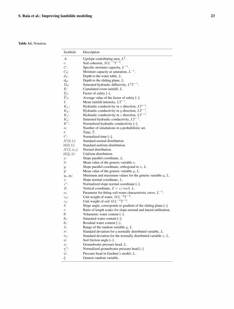
S. Raia et al.: Improving landslide modeling 23
Table A1. Notation.
Symbols Description
A: Upslope contributing area, L2.c: Soil cohesion, ML−1T−2.C: Specific moisture capacity, L−1.C0: Moisture capacity at saturation, L−1.dw: Depth to the water table, L.dfp: Depth to the sliding plane, L.D0: Saturated hydraulic diffusivity, L2T−1.E: Cumulated event rainfall, L.FS: Factor of safety [–].F S: Average value of the factor of safety [–].I: Mean rainfall intensity, LT−1.Kx: Hydraulic conductivity in x direction, LT−1.Ky: Hydraulic conductivity in y direction, LT−1.Kz: Hydraulic conductivity in z direction, LT−1.Ks: Saturated hydraulic conductivity, LT−1.K∗: Normalized hydraulic conductivity [–].n: Number of simulations in a probabilistic set.t: Time, T .t∗: Normalized time [–].N (0,1): Standard normal distribution.U(0,1): Standard uniform distribution.N (x,σx): Normal distribution.U(y,λ): Uniform distribution.x: Slope parallel coordinate, L.x: Mean value of the generic variable x.y: Slope parallel coordinate, orthogonal to x, L.y: Mean value of the generic variable y, L.ya,yb: Minimum and maximum values for the generic variable y, L.z: Slope normal coordinate, L.z∗: Normalized slope normal coordinate [–].Z: Vertical coordinate, Z = z/cosδ, L.α: Parameter for fitting soil-water characteristic curve, L−1.γw: Unit weight of water, ML−2T−2.γs: Unit weight of soil ML−2T−2.δ: Slope angle, corresponds to gradient of the sliding plane [–].ε: Ratio of length scales for slope-normal and lateral infiltration.θ: Volumetric water content [–].θs: Saturated water content [–].θr: Residual water content [–].λ: Range of the random variable y, L.σ: Standard deviation for a normally distributed variable, L.σx: Standard deviation for the normally distributed variable x, L.φ: Soil friction angle [–].ψ: Groundwater pressure head, L.ψ∗: Normalized groundwater pressure head [–].ψ: Pressure head in Gardner’s model, L.ξ: Generic random variable.
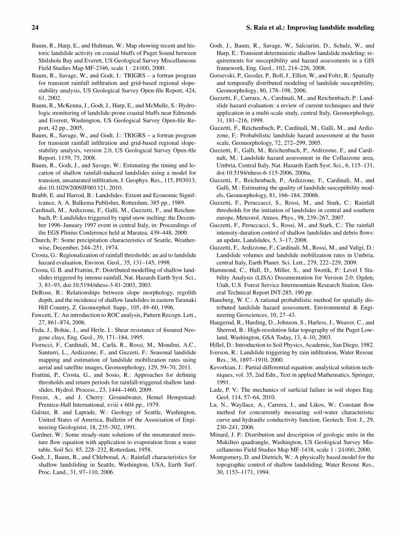
24 S. Raia et al.: Improving landslide modeling
Baum, R., Harp, E., and Hultman, W.: Map showing recent and his-toric landslide activity on coastal bluffs of Puget Sound betweenShilshole Bay and Everett, US Geological Survey MiscellaneousField Studies Map MF-2346, scale 1 : 24000, 2000.
Baum, R., Savage, W., and Godt, J.: TRIGRS – a fortran programfor transient rainfall infiltration and grid-based regional slope-stability analysis, US Geological Survey Open-file Report, 424,61, 2002.
Baum, R., McKenna, J., Godt, J., Harp, E., and McMulle, S.: Hydro-logic monitoring of landslide-prone coastal bluffs near Edmondsand Everett, Washington, US Geological Survey Open-file Re-port, 42 pp., 2005.
Baum, R., Savage, W., and Godt, J.: TRIGRS – a fortran programfor transient rainfall infiltration and grid-based regional slope-stability analysis, version 2.0, US Geological Survey Open-fileReport, 1159, 75, 2008.
Baum, R., Godt, J., and Savage, W.: Estimating the timing and lo-cation of shallow rainfall-induced landslides using a model fortransient, unsaturated infiltration, J. Geophys. Res., 115, F03013,doi:10.1029/2009JF001321, 2010.
Brabb, E. and Harrod, B.: Landslides: Extent and Economic Signif-icance, A. A. Balkema Publisher, Rotterdam, 385 pp., 1989.
Cardinali, M., Ardizzone, F., Galli, M., Guzzetti, F., and Reichen-bach, P.: Landslides triggered by rapid snow melting: the Decem-ber 1996–January 1997 event in central Italy, in: Proceedings ofthe EGS Plinius Conference held at Maratea, 439–448, 2000.
Church, P.: Some precipitation characteristics of Seattle, Weather-wise, December, 244–251, 1974.
Crosta, G.: Regionalization of rainfall thresholds: an aid to landslidehazard evaluation, Environ. Geol., 35, 131–145, 1998.
Crosta, G. B. and Frattini, P.: Distributed modelling of shallow land-slides triggered by intense rainfall, Nat. Hazards Earth Syst. Sci.,3, 81–93, doi:10.5194/nhess-3-81-2003, 2003.
DeRose, R.: Relationships between slope morphology, regolithdepth, and the incidence of shallow landslides in eastern TaranakiHill Country, Z. Geomorphol. Supp., 105, 49–60, 1996.
Fawcett, T.: An introduction to ROC analysis, Pattern Recogn. Lett.,27, 861–874, 2006.
Feda, J., Bohac, J., and Herle, I.: Shear resistance of fissured Neo-gene clays, Eng. Geol., 39, 171–184, 1995.
Fiorucci, F., Cardinali, M., Carla, R., Rossi, M., Mondini, A.C.,Santurri, L., Ardizzone, F., and Guzzeti, F.: Seasonal landslidemapping and estimation of landslide mobilization rates usingaerial and satellite images, Geomorphology, 129, 59–70, 2011.
Frattini, P., Crosta, G., and Sosio, R.: Approaches for definingthresholds and return periods for rainfall-triggered shallow land-slides, Hydrol. Process., 23, 1444–1460, 2009.
Freeze, A., and J. Cherry: Groundwater, Hemel Hempstead:Prentice-Hall International, xviii + 604 pp., 1979.
Galster, R. and Laprade, W.: Geology of Seattle, Washington,United States of America, Bulletin of the Association of Engi-neering Geologistst, 18, 235–302, 1991.
Gardner, W.: Some steady-state solutions of the unsaturated mois-ture flow equation with application to evaporation from a watertable, Soil Sci. 85, 228–232, Rotterdam, 1958.
Godt, J., Baum, R., and Chleborad, A.: Rainfall characteristics forshallow landsliding in Seattle, Washington, USA, Earth Surf.Proc. Land., 31, 97–110, 2006.
Godt, J., Baum, R., Savage, W., Salciarini, D., Schulz, W., andHarp, E.: Transient deterministic shallow landslide modeling: re-quirements for susceptibility and hazard assessments in a GISframework, Eng. Geol., 102, 214–226, 2008.
Gorsevski, P., Gessler, P., Boll, J., Elliot, W., and Foltz, R.: Spatiallyand temporally distributed modeling of landslide susceptibility,Geomorphology, 80, 178–198, 2006.
Guzzetti, F., Carrara, A., Cardinali, M., and Reichenbach, P.: Land-slide hazard evaluation: a review of current techniques and theirapplication in a multi-scale study, central Italy, Geomorphology,31, 181–216, 1999.
Guzzetti, F., Reichenbach, P., Cardinali, M., Galli, M., and Ardiz-zone, F.: Probabilistic landslide hazard assessment at the basinscale, Geomorphology, 72, 272–299, 2005.
Guzzetti, F., Galli, M., Reichenbach, P., Ardizzone, F., and Cardi-nali, M.: Landslide hazard assessment in the Collazzone area,Umbria, Central Italy, Nat. Hazards Earth Syst. Sci., 6, 115–131,doi:10.5194/nhess-6-115-2006, 2006a.
Guzzetti, F., Reichenbach, P., Ardizzone, F., Cardinali, M., andGalli, M.: Estimating the quality of landslide susceptibility mod-els, Geomorphology, 81, 166–184, 2006b.
Guzzetti, F., Peruccacci, S., Rossi, M., and Stark, C.: Rainfallthresholds for the initiation of landslides in central and southerneurope, Meteorol. Atmos. Phys., 98, 239–267, 2007.
Guzzetti, F., Peruccacci, S., Rossi, M., and Stark, C.: The rainfallintensity-duration control of shallow landslides and debris flows:an update, Landslides, 5, 3–17, 2008.
Guzzetti, F., Ardizzone, F., Cardinali, M., Rossi, M., and Valigi, D.:Landslide volumes and landslide mobilization rates in Umbria,central Italy, Earth Planet. Sci. Lett., 279, 222–229, 2009.
Hammond, C., Hall, D., Miller, S., and Swetik, P.: Level I Sta-bility Analysis (LISA) Documentation for Version 2.0: Ogden,Utah, U.S. Forest Service Intermountain Research Station, Gen-eral Technical Report INT-285, 190 pp.
Haneberg, W. C.: A rational probabilistic method for spatially dis-tributed landslide hazard assessment, Environmental & Engi-neering Geosciences, 10, 27–43.
Haugerud, R., Harding, D., Johnson, S., Harless, J., Weaver, C., andSherrod, B.: High-resolution lidar topography of the Puget Low-land, Washington, GSA Today, 13, 4–10, 2003.
Hillel, D.: Introduction to Soil Physics, Academic, San Diego, 1982.Iverson, R.: Landslide triggering by rain infiltration, Water Resour.
Res., 36, 1897–1910, 2000.Kevorkian, J.: Partial differential equation: analytical solution tech-
niques, vol. 35, 2nd Edn., Text in applied Mathematics, Springer,1991.
Lade, P. V.: The mechanics of surficial failure in soil slopes Eng.Geol. 114, 57–64, 2010.
Lu, N., Wayllace, A., Carrera, J., and Likos, W.: Constant flowmethod for concurrently measuring soil-water characteristiccurve and hydraulic conductivity function, Geotech. Test. J., 29,230–241, 2006.
Minard, J. P.: Distribution and description of geologic units in theMukilteo quadrangle, Washington, US Geological Survey Mis-cellaneous Field Studies Map MF-1438, scale 1 : 24000, 2000.
Montgomery, D. and Dietrich, W.: A physically based model for thetopographic control of shallow landsliding, Water Resour. Res.,30, 1153–1171, 1994.
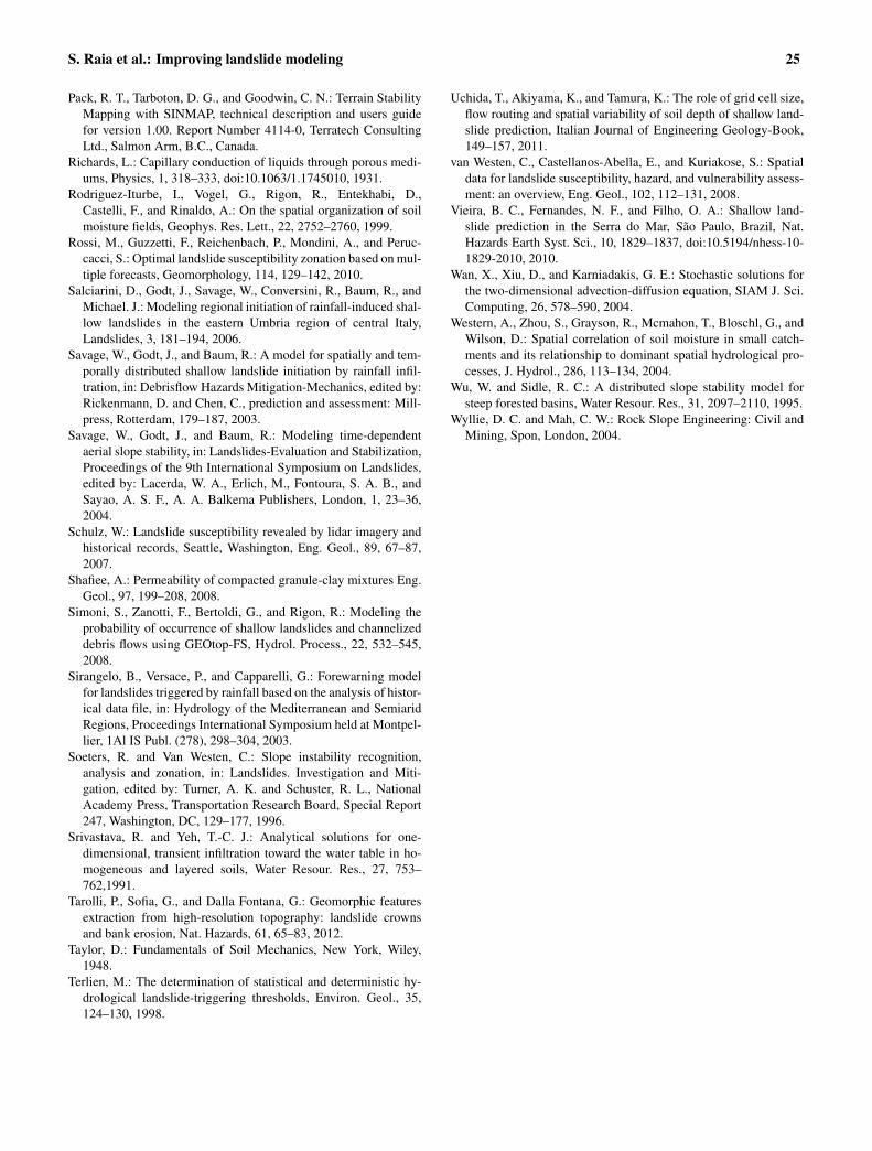
S. Raia et al.: Improving landslide modeling 25
Pack, R. T., Tarboton, D. G., and Goodwin, C. N.: Terrain StabilityMapping with SINMAP, technical description and users guidefor version 1.00. Report Number 4114-0, Terratech ConsultingLtd., Salmon Arm, B.C., Canada.
Richards, L.: Capillary conduction of liquids through porous medi-ums, Physics, 1, 318–333, doi:10.1063/1.1745010, 1931.
Rodriguez-Iturbe, I., Vogel, G., Rigon, R., Entekhabi, D.,Castelli, F., and Rinaldo, A.: On the spatial organization of soilmoisture fields, Geophys. Res. Lett., 22, 2752–2760, 1999.
Rossi, M., Guzzetti, F., Reichenbach, P., Mondini, A., and Peruc-cacci, S.: Optimal landslide susceptibility zonation based on mul-tiple forecasts, Geomorphology, 114, 129–142, 2010.
Salciarini, D., Godt, J., Savage, W., Conversini, R., Baum, R., andMichael. J.: Modeling regional initiation of rainfall-induced shal-low landslides in the eastern Umbria region of central Italy,Landslides, 3, 181–194, 2006.
Savage, W., Godt, J., and Baum, R.: A model for spatially and tem-porally distributed shallow landslide initiation by rainfall infil-tration, in: Debrisflow Hazards Mitigation-Mechanics, edited by:Rickenmann, D. and Chen, C., prediction and assessment: Mill-press, Rotterdam, 179–187, 2003.
Savage, W., Godt, J., and Baum, R.: Modeling time-dependentaerial slope stability, in: Landslides-Evaluation and Stabilization,Proceedings of the 9th International Symposium on Landslides,edited by: Lacerda, W. A., Erlich, M., Fontoura, S. A. B., andSayao, A. S. F., A. A. Balkema Publishers, London, 1, 23–36,2004.
Schulz, W.: Landslide susceptibility revealed by lidar imagery andhistorical records, Seattle, Washington, Eng. Geol., 89, 67–87,2007.
Shafiee, A.: Permeability of compacted granule-clay mixtures Eng.Geol., 97, 199–208, 2008.
Simoni, S., Zanotti, F., Bertoldi, G., and Rigon, R.: Modeling theprobability of occurrence of shallow landslides and channelizeddebris flows using GEOtop-FS, Hydrol. Process., 22, 532–545,2008.
Sirangelo, B., Versace, P., and Capparelli, G.: Forewarning modelfor landslides triggered by rainfall based on the analysis of histor-ical data file, in: Hydrology of the Mediterranean and SemiaridRegions, Proceedings International Symposium held at Montpel-lier, 1Al IS Publ. (278), 298–304, 2003.
Soeters, R. and Van Westen, C.: Slope instability recognition,analysis and zonation, in: Landslides. Investigation and Miti-gation, edited by: Turner, A. K. and Schuster, R. L., NationalAcademy Press, Transportation Research Board, Special Report247, Washington, DC, 129–177, 1996.
Srivastava, R. and Yeh, T.-C. J.: Analytical solutions for one-dimensional, transient infiltration toward the water table in ho-mogeneous and layered soils, Water Resour. Res., 27, 753–762,1991.
Tarolli, P., Sofia, G., and Dalla Fontana, G.: Geomorphic featuresextraction from high-resolution topography: landslide crownsand bank erosion, Nat. Hazards, 61, 65–83, 2012.
Taylor, D.: Fundamentals of Soil Mechanics, New York, Wiley,1948.
Terlien, M.: The determination of statistical and deterministic hy-drological landslide-triggering thresholds, Environ. Geol., 35,124–130, 1998.
Uchida, T., Akiyama, K., and Tamura, K.: The role of grid cell size,flow routing and spatial variability of soil depth of shallow land-slide prediction, Italian Journal of Engineering Geology-Book,149–157, 2011.
van Westen, C., Castellanos-Abella, E., and Kuriakose, S.: Spatialdata for landslide susceptibility, hazard, and vulnerability assess-ment: an overview, Eng. Geol., 102, 112–131, 2008.
Vieira, B. C., Fernandes, N. F., and Filho, O. A.: Shallow land-slide prediction in the Serra do Mar, Sao Paulo, Brazil, Nat.Hazards Earth Syst. Sci., 10, 1829–1837, doi:10.5194/nhess-10-1829-2010, 2010.
Wan, X., Xiu, D., and Karniadakis, G. E.: Stochastic solutions forthe two-dimensional advection-diffusion equation, SIAM J. Sci.Computing, 26, 578–590, 2004.
Western, A., Zhou, S., Grayson, R., Mcmahon, T., Bloschl, G., andWilson, D.: Spatial correlation of soil moisture in small catch-ments and its relationship to dominant spatial hydrological pro-cesses, J. Hydrol., 286, 113–134, 2004.
Wu, W. and Sidle, R. C.: A distributed slope stability model forsteep forested basins, Water Resour. Res., 31, 2097–2110, 1995.
Wyllie, D. C. and Mah, C. W.: Rock Slope Engineering: Civil andMining, Spon, London, 2004.