Shaft Deflection—A Very, Very Long Example
13
2013 ASEE Southeast Section Conference Shaft Deflection—A Very, Very Long Example Christopher D. Wilson 1 , Michael W. Renfro 2 Abstract – Most textbooks in mechanics of materials and components of machine describe numerous methods for determining shaft (beam) deflections. The examples are quite varied, but most are not interrelated with follow-up examples in which the same problem is attacked using different methods. Further, most examples are worked out by hand and do not emphasize numerical methods used in common practice. Here, the deflection of a stepped shaft in bending was solved using the following methods: closed-form successive integration of the bending moment equations, Castigliano’s second theorem, numerical successive integration using the trapezoid rule, finite element method, and estimation by beam table superposition. Computational tools, such as MATLAB, Excel, and Maple were used in the solution process. The advantages and disadvantages of the methods used are discussed as well as observations from use of the example. Keywords: beam deflection, Castigliano’s second theorem, double integration, finite element modeling, numerical integration I NTRODUCTION The basic idea of this paper is to present, or at least, outline the solution to a shaft deflection problem using several different methods. Studying the same problem from multiple perspectives is one way to gain a better overall understanding. Different problem solving strategies can lead to the same solution and allow a student to see how useful one method is when compared to another. Two other benefits from using different methods to study the same problem are confidence building and estimation-skill development. Certainly, if students have successfully arrived at one solution to a problem, they are likely to be more confident when trying another method. Also, having worked through the several different methods, students can begin to judge situations where one solution method might be preferred over others. Sometimes, the other method or methods may be not as accurate or as useful, but they can provide enough accuracy for estimating the solution. Students need to practice the art of estimation so that they can validate their own solutions. In this paper, we will consider only the statically determinate problem. However, the same methods could be applied to a statically indeterminate problem. Also, bending is restricted to a single plane in this paper. There are many different solution methods for beam/shaft deflections. Integration schemes—both direct successive integration and graphical integration—are the primary methods taught in mechanics of materials. Energy methods are very powerful, but often have less emphasis in the first mechanics of materials course. The general advice we give in machine design practice is to superimpose solutions from beam tables if the beam or shaft has a constant cross section. When a stepped shaft is to be studied, direct successive integration becomes tedious. For a stepped shaft, we recommend an energy method, such as Castigliano’s second theorem, if the deflection or slope is required at only a few locations. Otherwise, we recommend numerical methods, such as successive numerical integration or finite elements. However, we always recommend using beam table superposition for bounding estimates. There are many mechanics of materials texts available to students. Timoshenko [1] and Popov [2] are the classics in the field. Beer [3], Higdon [4] and Riley [5] are long established. Philpot [6], Vable [7] and Allen [8] are newer treatments. These texts provide many excellent examples of both statically determinate and indeterminate beam 1 Department of Mechanical Engineering, Tennessee Technological University. Box 5014, Cookeville, TN 38505. <[email protected]> 2 Center for Manufacturing Research, Tennessee Technological University. Box 5077, Cookeville, TN 38505. <[email protected]> © American Society for Engineering Education, 2013
-
Upload
hoangxuyen -
Category
Documents
-
view
223 -
download
0
Transcript of Shaft Deflection—A Very, Very Long Example
2013 ASEE Southeast Section Conference
Shaft Deflection—A Very, Very Long ExampleChristopher D. Wilson1, Michael W. Renfro2
Abstract – Most textbooks in mechanics of materials and components of machine describe numerous methods fordetermining shaft (beam) deflections. The examples are quite varied, but most are not interrelated with follow-upexamples in which the same problem is attacked using different methods. Further, most examples are worked out byhand and do not emphasize numerical methods used in common practice. Here, the deflection of a stepped shaft inbending was solved using the following methods: closed-form successive integration of the bending momentequations, Castigliano’s second theorem, numerical successive integration using the trapezoid rule, finite elementmethod, and estimation by beam table superposition. Computational tools, such as MATLAB, Excel, and Maplewere used in the solution process. The advantages and disadvantages of the methods used are discussed as well asobservations from use of the example.Keywords: beam deflection, Castigliano’s second theorem, double integration, finite element modeling, numericalintegration
INTRODUCTION
The basic idea of this paper is to present, or at least, outline the solution to a shaft deflection problem using severaldifferent methods. Studying the same problem from multiple perspectives is one way to gain a better overallunderstanding. Different problem solving strategies can lead to the same solution and allow a student to see howuseful one method is when compared to another. Two other benefits from using different methods to study the sameproblem are confidence building and estimation-skill development. Certainly, if students have successfully arrived atone solution to a problem, they are likely to be more confident when trying another method. Also, having workedthrough the several different methods, students can begin to judge situations where one solution method might bepreferred over others. Sometimes, the other method or methods may be not as accurate or as useful, but they canprovide enough accuracy for estimating the solution. Students need to practice the art of estimation so that they canvalidate their own solutions.
In this paper, we will consider only the statically determinate problem. However, the same methods could be appliedto a statically indeterminate problem. Also, bending is restricted to a single plane in this paper.
There are many different solution methods for beam/shaft deflections. Integration schemes—both direct successiveintegration and graphical integration—are the primary methods taught in mechanics of materials. Energy methodsare very powerful, but often have less emphasis in the first mechanics of materials course. The general advice wegive in machine design practice is to superimpose solutions from beam tables if the beam or shaft has a constantcross section. When a stepped shaft is to be studied, direct successive integration becomes tedious. For a steppedshaft, we recommend an energy method, such as Castigliano’s second theorem, if the deflection or slope is requiredat only a few locations. Otherwise, we recommend numerical methods, such as successive numerical integration orfinite elements. However, we always recommend using beam table superposition for bounding estimates.
There are many mechanics of materials texts available to students. Timoshenko [1] and Popov [2] are the classics inthe field. Beer [3], Higdon [4] and Riley [5] are long established. Philpot [6], Vable [7] and Allen [8] are newertreatments. These texts provide many excellent examples of both statically determinate and indeterminate beam
1Department of Mechanical Engineering, Tennessee Technological University. Box 5014, Cookeville, TN38505. <[email protected]>
2Center for Manufacturing Research, Tennessee Technological University. Box 5077, Cookeville, TN 38505.<[email protected]>
© American Society for Engineering Education, 2013
2013 ASEE Southeast Section Conference
problems. A variety of methods are used. For example, Hibbeler’s [9] chapter “Deflections of Beams and Shafts”includes successive integration of the load intensity and successive integration of the bending moment, singularity(Macaulay) functions, the moment-area method, and the principle of superposition. In a later chapter, “EnergyMethods,” virtual work and Castigliano’s second theorem are used to determine deflections.
As with mechanics of materials, there are many component machine design texts. All these texts assume thatstudents have already taken a course in mechanics of materials. Shigley[10], Phelan [11] and Spotts [12] are notableclassics, while Johnson [13] provided a new approach. Newer entries include Norton [14], Ugural [15] and Collins[16]. All these texts assume that students have taken mechanics of materials. This assumption is also true of mostmachine design courses.
There are many different tools for solving such problems. Powerful graphing calculators often have symbolic andnumerical capabilities for solving differential equations and for integration. Computer software includes specialtyeducational programs for mechanics of materials, small locally-written finite element codes, commercial finiteelement codes, computer algebra systems and related mathematical analysis programs and spreadsheets. With allthese computer tools available, many faculty and students will still choose to write their code.
THE PROBLEM STATEMENT
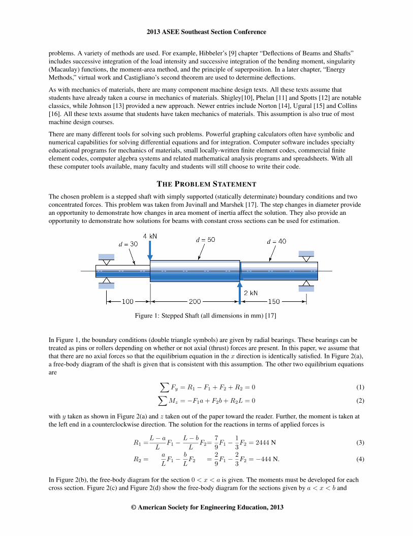
The chosen problem is a stepped shaft with simply supported (statically determinate) boundary conditions and twoconcentrated forces. This problem was taken from Juvinall and Marshek [17]. The step changes in diameter providean opportunity to demonstrate how changes in area moment of inertia affect the solution. They also provide anopportunity to demonstrate how solutions for beams with constant cross sections can be used for estimation.
Figure 1: Stepped Shaft (all dimensions in mm) [17]
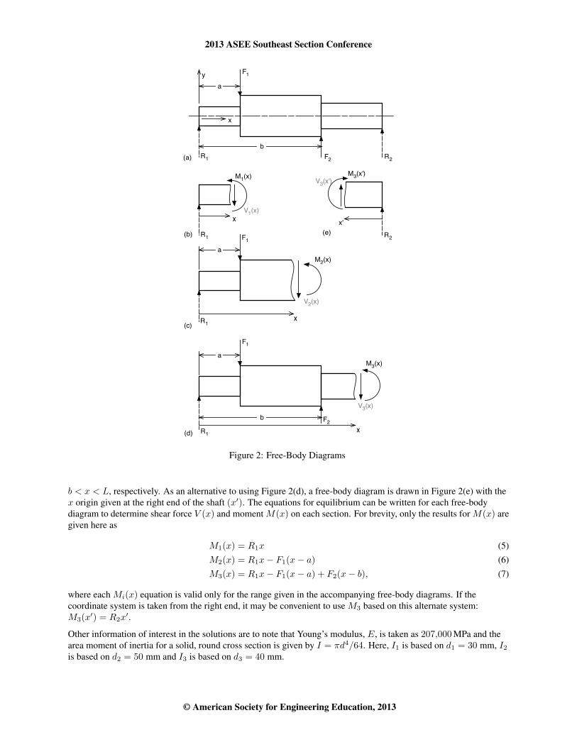
In Figure 1, the boundary conditions (double triangle symbols) are given by radial bearings. These bearings can betreated as pins or rollers depending on whether or not axial (thrust) forces are present. In this paper, we assume thatthat there are no axial forces so that the equilibrium equation in the x direction is identically satisfied. In Figure 2(a),a free-body diagram of the shaft is given that is consistent with this assumption. The other two equilibrium equationsare ∑
Fy = R1 − F1 + F2 +R2 = 0 (1)∑Mz = −F1a+ F2b+R2L = 0 (2)
with y taken as shown in Figure 2(a) and z taken out of the paper toward the reader. Further, the moment is taken atthe left end in a counterclockwise direction. The solution for the reactions in terms of applied forces is
R1 =L− aL
F1 −L− bL
F2=7
9F1 −
1
3F2 = 2444 N (3)
R2 =a
LF1 −
b
LF2 =
2
9F1 −
2
3F2 = −444 N. (4)
In Figure 2(b), the free-body diagram for the section 0 < x < a is given. The moments must be developed for eachcross section. Figure 2(c) and Figure 2(d) show the free-body diagram for the sections given by a < x < b and
© American Society for Engineering Education, 2013
2013 ASEE Southeast Section Conference
y
x
x x'
x
x
F1
R1
R1
R2
R2
F2R1
R1
F1
F1
F2
M1(x)M3(x')
M3(x)
M2(x)
V1(x)
V2(x)
V3(x')
V3(x)
(a)
(b)
(c)
(d)
(e)
a
a
a
b
b
Figure 2: Free-Body Diagrams
b < x < L, respectively. As an alternative to using Figure 2(d), a free-body diagram is drawn in Figure 2(e) with thex origin given at the right end of the shaft (x′). The equations for equilibrium can be written for each free-bodydiagram to determine shear force V (x) and moment M(x) on each section. For brevity, only the results for M(x) aregiven here as
M1(x) = R1x (5)M2(x) = R1x− F1(x− a) (6)M3(x) = R1x− F1(x− a) + F2(x− b), (7)
where each Mi(x) equation is valid only for the range given in the accompanying free-body diagrams. If thecoordinate system is taken from the right end, it may be convenient to use M3 based on this alternate system:M3(x
′) = R2x′.
Other information of interest in the solutions are to note that Young’s modulus, E, is taken as 207,000MPa and thearea moment of inertia for a solid, round cross section is given by I = πd4/64. Here, I1 is based on d1 = 30 mm, I2is based on d2 = 50 mm and I3 is based on d3 = 40 mm.
© American Society for Engineering Education, 2013
2013 ASEE Southeast Section Conference
THE SOLUTIONS
Superposition from Beam Table (By Hand Estimate)
As stated, the problem cannot be directly solved using superposition of beam table solutions because the crosssection is stepped. However, the beam tables can be used to quickly determine an estimate for the solution—by handcalculation. The solution for a simply-supported beam with a single point force is given in all mechanics of materialsand machine design texts.
We must choose a constant diameter (or alternatively, choose a constant moment of inertia) in making thecalculations. Clearly, the 30 mm diameter is not representative of the entire shaft and we expect using it will lead tomuch larger deflections than the actual stepped shaft. The opposite thought comes to mind for the 50 mm diametershaft; we expect that using 50 mm will lead to much smaller deflections than the actual stepped shaft. Perhaps, the 40mm diameter is a good choice. For it, we expect a deflection that is smaller than the actual deflection for the leftmostpart of the shaft. We also expect that the estimated deflection for the rightmost part of the shaft will be close to theactual deflection. Frankly, it is simple enough to try all three diameters and students should be encouraged to do so.
Successive Integration (Exact)
The successive integration of the moment equations requires three intervals. For each interval, there will be twoconstants of integration. Thus, there are six constants of integration to be found. For the simply-supported shaft, theboundary conditions v(0) = 0 and v(L) = 0 will provide two equations. Four additional equations are needed. Theycome from compatibility conditions at the intersections of the three intervals. At the left intersection, x = a, we musthave v(a)left = v(a)right and v′(a)left = v′(a)right. At the rightmost intersection, x = b, we must havev(b)left = v(b)right and v′(b)left = v′(b)right.
From Figure 2, the moments can be integrated to yield slope and deflection equations. The integration results aresummarized here. For 0 < x < a,
M1(x) = R1x (8)∫M1(x)dx = EI1
dv1dx
= R1x2
2+ C1 (9)∫∫
M1(x)dx = EI1v1(x) = R1x3
6+ C1x+ C2. (10)
For a < x < b,
M2(x) = R1x− F1(x− a) (11)∫M2(x)dx = EI2
dv1dx
= R1x2
2− F1
(x− a)2
2+ C3 (12)∫∫
M2(x)dx = EI2v2(x) = R1x3
6− F1
(x− a)3
6+ C3x+ C4. (13)
For b < x < L,
M3(x) = R1x− F1(x− a) + F2(x− b) (14)∫M3(x)dx = EI3
dv1dx
= R1x2
2− F1
(x− a)2
2+ F2
(x− b)2
2+ C5 (15)∫∫
M3(x)dx = EI3v3(x) = R1x3
6− F1
(x− a)3
6+ F2
(x− b)3
6+ C5x+ C6. (16)
Here, the flexural rigidity EI and odd-subscripted constants C1, C3 and C5 have the dimensions of F × L2 and theunits of N×mm2. Then even-subscripted constants C2, C4 and C6 have the dimensions of F × L3 and units ofN×mm3.
Substituting x = 0 clearly yields EI1v1(0) = C2. But, v1(0) = 0, so C2 = 0. The other five conditions can be
© American Society for Engineering Education, 2013
2013 ASEE Southeast Section Conference
written in matrix form as
0 0 0 L 1
a − aα2
− 1α2
0 0
1 − 1α2
0 0 0
0 bα2
1α2
− bα3
− 1α3
0 1α2
0 − 1α3
0
C1
C3
C4
C5
C6
=
−R1L3
6 + F1(L−a)3
6 − F2(L−b)3
6(1α2− 1)R1
a3
6(1α2− 1)R1
a2
2(1α3− 1
α2
) [R1
b3
6 − F1(b−a)3
6
](
1α3− 1
α2
) [R1
b2
2 − F1(b−a)2
2
]
. (17)
where α2 = I2/I1 and α3 = I3/I1. Note that Young’s modulus E cancels out of the equations and does not appearin the above matrix. A brief MATLAB script for the successive integration method is given in Listing 1.
Castigliano’s Second Theorem (Exact)
Castigliano’s Second Theorem is a commonly used energy method. However, it is limited to finding the deflection ata single point. It requires a point force at the location of interest, but a fictitious point force can be used if the locationdoes not have a point force. From Equations 5 through 7, we substitute the reaction equations 3-4 to yield:
M1(x) =
(7
9F1 −
1
3F2
)x (18)
M2(x) =
(7
9F1 −
1
3F2
)x− F1(x− a) (19)
M3(x) =
(7
9F1 −
1
3F2
)x− F1(x− a) + F2(x− b). (20)
Castigliano’s Second Theorem requires partial derivatives of the moment equations with respect to the point force atthe location of interest. If we use the method to determine the deflection at both x = a (where F1 is located) andx = b (where F2 is located), the following derivatives will be needed:
∂M
∂F1=
79x 0 < x < a79x− (x− a) a < x < b79x− (x− a) b < x < L
(21)
∂M
∂F2=
−x3 0 < x < a
−x3 a < x < b
−x3 + (x− b) b < x < L.
(22)
The resulting equations for the deflections are
v(a) =
∫ a
0
M1
EI1
∂M1
∂F1dx+
∫ b
a
M2
EI2
∂M2
∂F1dx+
∫ L
b
M3
EI3
∂M3
∂F1dx (23)
and
v(b) =
∫ a
0
M1
EI1
∂M1
∂F2dx+
∫ b
a
M2
EI2
∂M2
∂F2dx+
∫ L
b
M3
EI3
∂M3
∂F2dx. (24)
The equations are implemented in a Maple script given in Listing 2. It is very important to to note to students thatCastigliano’s Second Theorem gives v(b) as a negative value because the deflection is in the opposite direction of F2.They must see that F1 is downward and is twice as large as the upward F2, so that the overall deflection at x = b isstill downward (negative).
The Maple script also includes the use of a fictitious force that can be varied in a < x < b to determine deflections inthat range. Thus, using a script makes the effort involved in Castigliano’s Second Theorem more valuable.
© American Society for Engineering Education, 2013
2013 ASEE Southeast Section Conference
Finite Element Method (Numerical Estimate)
The finite element method, described by Mueller [18] and many others, is a procedure that first decomposes aphysical system into a set of simpler elements. Each element is governed by a simple system of algebraic equations.The elements are reassembled into an approximation of the original system, and the resulting system of equations issolved with matrix algebra. In the case of a structure subjected to loads within the linear elastic region of thematerial, each element is modeled as a linear elastic member with a governing equation of
{f}(e) = [k](e) {u}(e) , (25)
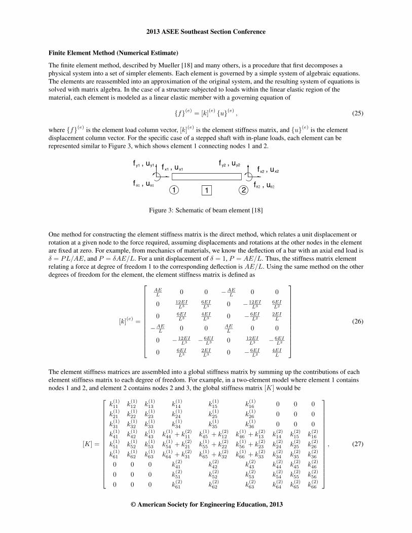
where {f}(e) is the element load column vector, [k](e) is the element stiffness matrix, and {u}(e) is the elementdisplacement column vector. For the specific case of a stepped shaft with in-plane loads, each element can berepresented similar to Figure 3, which shows element 1 connecting nodes 1 and 2.
f , uy1
21 1f , uθ1
f , uy2 f , ux2
θ2f , uθ2θ1
x1f , ux1y2
x2y1
Figure 3: Schematic of beam element [18]
One method for constructing the element stiffness matrix is the direct method, which relates a unit displacement orrotation at a given node to the force required, assuming displacements and rotations at the other nodes in the elementare fixed at zero. For example, from mechanics of materials, we know the deflection of a bar with an axial end load isδ = PL/AE, and P = δAE/L. For a unit displacement of δ = 1, P = AE/L. Thus, the stiffness matrix elementrelating a force at degree of freedom 1 to the corresponding deflection is AE/L. Using the same method on the otherdegrees of freedom for the element, the element stiffness matrix is defined as
[k](e)
=
AEL 0 0 −AEL 0 0
0 12EIL3
6EIL3 0 − 12EI
L36EIL2
0 6EIL3
4EIL3 0 − 6EI
L22EIL
−AEL 0 0 AEL 0 0
0 − 12EIL3 − 6EI
L3 0 12EIL3 − 6EI
L2
0 6EIL3
2EIL3 0 − 6EI
L24EIL
(26)
The element stiffness matrices are assembled into a global stiffness matrix by summing up the contributions of eachelement stiffness matrix to each degree of freedom. For example, in a two-element model where element 1 containsnodes 1 and 2, and element 2 contains nodes 2 and 3, the global stiffness matrix [K] would be
[K] =
k(1)11 k
(1)12 k
(1)13 k
(1)14 k
(1)15 k
(1)16 0 0 0
k(1)21 k
(1)22 k
(1)23 k
(1)24 k
(1)25 k
(1)26 0 0 0
k(1)31 k
(1)32 k
(1)33 k
(1)34 k
(1)35 k
(1)36 0 0 0
k(1)41 k
(1)42 k
(1)43 k
(1)44 + k
(2)11 k
(1)45 + k
(2)12 k
(1)46 + k
(2)13 k
(2)14 k
(2)15 k
(2)16
k(1)51 k
(1)52 k
(1)53 k
(1)54 + k
(2)21 k
(1)55 + k
(2)22 k
(1)56 + k
(2)23 k
(2)24 k
(2)25 k
(2)26
k(1)61 k
(1)62 k
(1)63 k
(1)64 + k
(2)31 k
(1)65 + k
(2)32 k
(1)66 + k
(2)33 k
(2)34 k
(2)35 k
(2)36
0 0 0 k(2)41 k
(2)42 k
(2)43 k
(2)44 k
(2)45 k
(2)46
0 0 0 k(2)51 k
(2)52 k
(2)53 k
(2)54 k
(2)55 k
(2)56
0 0 0 k(2)61 k
(2)62 k
(2)63 k
(2)64 k
(2)65 k
(2)66
, (27)
© American Society for Engineering Education, 2013

2013 ASEE Southeast Section Conference
0 50 100 150 200 250 300 350 400 450−0.1
−0.09
−0.08
−0.07
−0.06
−0.05
−0.04
−0.03
−0.02
−0.01
0
Position from left end (mm)
Deflection (
mm
)
Coarse FEM (3 elements)
Coarse FEM cubic interpolation
Medium FEM (9 elements)
Medium FEM cubic interpolation
Fine FEM (18 elements)
Fine FEM cubic interpolation
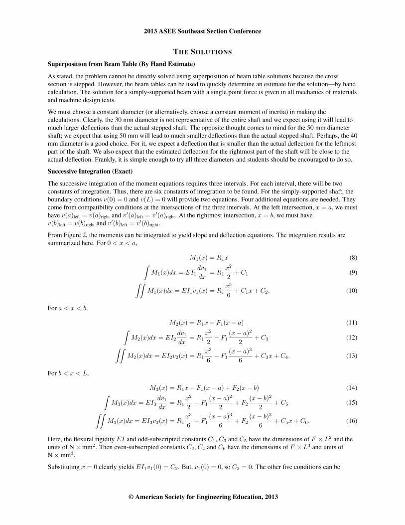
Figure 4: Influence of element length on shaft deflection
where k(m)ij represents the ith row and jth column of the stiffness matrix for element m.
Once the global stiffness matrix is assembled, the global force and displacement vectors ({F} and {U}) areconstructed. Each vector is a list of known and unknown forces and displacements sorted by degree of freedom.Since the first goal of the finite element method is to solve for the unknown displacements, all items in the stiffness,force, and displacement matrices corresponding to known displacements must be eliminated. For example, if node1’s y displacement (corresponding to degree of freedom 2) is fixed, then row 2 of the global force and displacementvectors must be eliminated, along with row 2 and column 2 of the global stiffness matrix.
Now that the global matrices and vectors contain only unknown displacements, the system of equations can be solvedfor {U}. Any method for solving a system of equations {F} = [K]{U} for {U} is acceptable, but Gaussianelimination or LU decomposition are popular methods. A MATLAB script demonstrating this procedure, adaptedfrom [18], is given in Listing 3. The mesh provided in the script uses an element length of 50 mm for a total of nineelements. This discretization is fine enough to provide an excellent match to the successive integration andCastigliano’s solutions. The script should be reused with fewer elements (perhaps three elements of unequal length)and with a larger number of elements (perhaps 18 elements of a uniform length of 25 mm) to demonstrate theconvergence process, as shown in Figure 4.
EXPERIENCE, RESULTS SUMMARY AND CONCLUSIONS
The first author’s experience with the example problem in a machine design course has been very successful.Students appreciate having a second (or third or even fourth) chance to successfully solve a problem. The examplehas been given to the class in three ways. First, the example has been used as an in-class case study spanning parts oflectures over a three-week period of studying design for stiffness principles. The total time expended for the examplegiven here is approximately three hours (approximately one-third of the total time allocated for design for stiffness in
© American Society for Engineering Education, 2013
2013 ASEE Southeast Section Conference
0 50 100 150 200 250 300 350 400 450−0.25
−0.2
−0.15
−0.1
−0.05
0
0.05
0.1
Position from left end (mm)
Deflection (
mm
)
Finite Element
Successive Integration
Castigliano’s Method
Superposition (30 mm shaft)
Superposition (40 mm shaft)
Superposition (50 mm shaft)
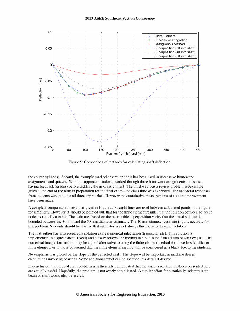
Figure 5: Comparison of methods for calculating shaft deflection
the course syllabus). Second, the example (and other similar ones) has been used in successive homeworkassignments and quizzes. With this approach, students worked through three homework assignments in a series,having feedback (grades) before tackling the next assignment. The third way was a review problem set/examplegiven at the end of the term in preparation for the final exam—no class time was expended. The anecdotal responsesfrom students was good for all three approaches. However, no quantitative measurements of student improvementhave been made.
A complete comparison of results is given in Figure 5. Straight lines are used between calculated points in the figurefor simplicity. However, it should be pointed out, that for the finite element results, that the solution between adjacentnodes is actually a cubic. The estimates based on the beam table superposition verify that the actual solution isbounded between the 30 mm and the 50 mm diameter estimates. The 40 mm diameter estimate is quite accurate forthis problem. Students should be warned that estimates are not always this close to the exact solution.
The first author has also prepared a solution using numerical integration (trapezoid rule). This solution isimplemented in a spreadsheet (Excel) and closely follows the method laid out in the fifth edition of Shigley [10]. Thenumerical integration method may be a good alternative to using the finite element method for those less familiar tofinite elements or to those concerned that the finite element method will be considered as a black-box to the students.
No emphasis was placed on the slope of the deflected shaft. The slope will be important in machine designcalculations involving bearings. Some additional effort can be spent on this detail if desired.
In conclusion, the stepped shaft problem is sufficiently complicated that the various solution methods presented hereare actually useful. Hopefully, the problem is not overly complicated. A similar effort for a statically indeterminatebeam or shaft would also be useful.
© American Society for Engineering Education, 2013
2013 ASEE Southeast Section Conference
REFERENCES
[1] Gere, James M. and Stephen P. Timoshenko. Mechanics of Materials. PWS, Boston, 1997.[2] Popov, Egor P. Mechanics of Materials. Prentice Hall, Upper Saddle River, New Jersey, 1976.[3] Beer, Ferdinand P., Jr. E. Russell Johnston, John T. DeWolf, and David F. Mazurek. Mechanics of Materials.
McGraw-Hill, New York, 2011.[4] Higdon, Archie, Edward H. Ohlsen, and William B. Stiles. Mechanics of Materials. Wiley, Hoboken, New
Jersey, 1960.[5] Riley, William F., Leroy D. Sturges, and Don H. Morris. Mechanics of Materials. Wiley, Hoboken, New Jersey,
2006.[6] Philpot, Timothy A. Mechanics of Materials: An Integrated Learning System. Wiley, Hoboken, New Jersey,
2012.[7] Vable, Madhukar. Mechanics of Materials. Oxford University Press, New York, 2002.[8] Allen, David H. Introduction to the Mechanics of Deformable Solids: Bars and Beams. Springer, Berlin, 2012.[9] Hibbeler, Russell C. Mechanics of Materials. Prentice Hall, Upper Saddle River, New Jersey, 2010.[10] Shigley, Joseph Edward and Charles Mischke. Mechanical Engineering Design. McGraw-Hill, New York,
1989.[11] Phelan, Richard M. Fundamentals of Mechanical Design. McGraw-Hill, New York, 1970.[12] Spotts, Merhyle F., Terry E. Shoup, and Lee E. Hornberger. Design of Machine Elements. Prentice Hall, Upper
Saddle River, New Jersey, 2003.[13] Johnson, Ray C. Optimum Design of Mechanical Elements. Wiley, New York, 1980.[14] Norton, Robert L. Machine Design. Prentice Hall, Upper Saddle River, New Jersey, 2010.[15] Ugural, Ansel C. Mechanical Design: An Integrated Approach. McGraw-Hill, New York, 2003.[16] Collins, Jack A., Henry R. Busby, and George H. Staab. Mechanical Design of Machine Elements and
Machines. Wiley, Hoboken, New Jersey, 2009.[17] Juvinall, Robert C. and Kurt M. Marshek. Fundamentals of Machine Component Design. Wiley, Hoboken,
New Jersey, 2011.[18] Donald W. Mueller, Jr. “Introducing the Finite Element Method to Mechanical Engineering Students Using
MATLAB.” In “Proceedings of the 2003 American Society for Engineering Education Annual Conference &Exposition,” American Society for Engineering Education, 2003.
Christopher D. Wilson
Christopher D. Wilson is an Associate Professor in mechanical engineering at Tennessee Technological University.He holds degrees in mechanical engineering (B.S., M.S.) from Tennessee Tech, mathematics (M.S.) from Universityof Alabama-Huntsville, and engineering science and mechanics (Ph.D.) from University of Tennessee-Knoxville. Histeaching and research interests are in machine design, mechanical behavior of materials, and computationalmechanics. He is a member of ASME, ASTM, ASEE, AIAA and is currently a vice-president of Pi Tau Sigma (thenational honor society for mechanical engineers).
Michael W. Renfro
Michael W. Renfro is a Research and Development Engineer for the Center for Manufacturing Research at TennesseeTechnological University. He holds degrees in mechanical engineering (B.S., M.S.) from Tennessee Tech, and is apart-time Ph.D. student there. His teaching and research interests include engineering graphics and solid modeling;engineering applications of MATLAB, LabVIEW, and Python; computational and experimental solid mechanics; andhigh performance computing.
© American Society for Engineering Education, 2013

2013 ASEE Southeast Section Conference
SUCESSIVE INTEGRATION CODE
Listing 1: MATLAB Script for Successive Integration% Successive integration method for stepped shaft
% Define the symbolic problemsyms x1 x2 x3 E L a b d1 d2 d3 F1 F2 c1 c2 c3 c4 c5 c6R1 = (L-a)/L*F1-(L-b)/L*F2;I1 = pi*d1^4/64;I2 = pi*d2^4/64;I3 = pi*d3^4/64;alpha2 = I2/I1;alpha3 = I3/I1;coeff = [ ...
0 0 0 L 1;a -a/alpha2 -1/alpha2 0 0;1 -1/alpha2 0 0 0;0 b/alpha2 1/alpha2 -b/alpha3 -1/alpha3;0 1/alpha2 0 -1/alpha3 0 ...];
rhs = [-R1*L^3/6+F1*(L-a)^3/6-F2*(L-b)^3/6;(1/alpha2-1)*R1*a^3/6;(1/alpha2-1)*R1*a^2/2;(1/alpha3-1/alpha2)*(R1*b^3/6-F1*(b-a)^3/6);(1/alpha3-1/alpha2)*(R1*b^2/2-F1*(b-a)^2/2)];
C = coeff\rhs; % elements of C1, C3, C4, C5, C6C = [C(1); 0; C(2:5)]; % elements of C1 ... C6v1 = (R1*(x1^3/6)+C(1)*x1+C(2))/(E*I1);v2 = (R1*(x2^3/6)-F1*(x2-a)^3/6+C(3)*x2+C(4))/(E*I2);v3 = (R1*(x3^3/6)-F1*(x3-a)^3/6+...
F2*(x3-b)^3/6+C(5)*x3+C(6))/(E*I3);
% Parameters for this particular stepped shaftL = 450; a = 100; b = 300;d1 = 30; d2 = 50; d3 = 40;F1 = 4000; F2 = 2000; E = 207e3;x1 = 0:25:a; x2 = a:25:b; x3 = b:25:L;% Evaluated solutionv1evaluated = subs(v1);v2evaluated = subs(v2);v3evaluated = subs(v3);plot(x1,v1evaluated,’-o’,x2,v2evaluated,’-s’,...
x3,v3evaluated,’-d’)xlabel(’Position along shaft (mm)’);ylabel(’Deflection (mm)’);grid on;table = [ x1 x2 x3; v1evaluated v2evaluated v3evaluated ]’
© American Society for Engineering Education, 2013
2013 ASEE Southeast Section Conference
CASTIGLIANO’S METHOD CODE
Listing 2: Maple Script for Castigliano’s Methodrestart;# Set up equilibrium equationsFy:=R1+R2-F1-F2-P:M0:=-F1*a-F2*b-P*c+R2*L:# Solve for reactionsR2:=solve(M0=0,R2);R1:=solve(Fy=0,R1);# Define moment diagramM1:=R1*x:M2:=M1-F1*(x-a):M3:=M2-P*(x-c):M4:=M3-F2*(x-b):# Take partials of moments with respect to PdM1dP:=diff(M1,P):dM2dP:=diff(M2,P):dM3dP:=diff(M3,P):dM4dP:=diff(M4,P):# Define deflection at P in terms of partial of strain energy with# respect to PvP:=int(M1/(E*I1)*dM1dP,x=0..a)+int(M2/(E*I2)*dM2dP,x=a..c)+ \
int(M3/(E*I2)*dM3dP,x=c..b)+int(M4/(E*I3)*dM4dP,x=b..L):# Define shaft geometry, material, and loadingd1:=30: d2:=50: d3:=40: a:=100: b:=300: L:=450:I1:=evalf(Pi)*d1^4/64: I2:=evalf(Pi)*d2^4/64: I3:=evalf(Pi)*d3^4/64:E:=207e3: F1:=4000: F2:=-2000: P:=0:# Evaluate deflection for given shaft and loadingfor c from a to b by 25 do
v:=evalf(vP);printf("x=%f, v=%f\n", c, v);
end do:
© American Society for Engineering Education, 2013
2013 ASEE Southeast Section Conference
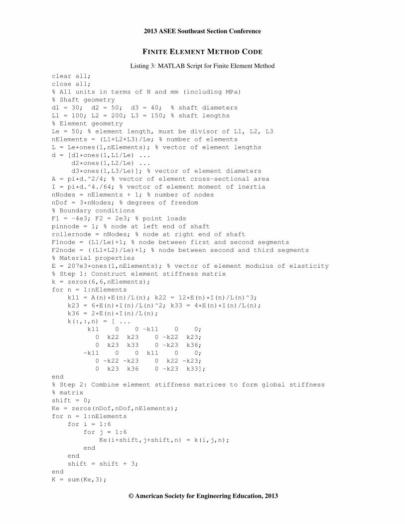
FINITE ELEMENT METHOD CODE
Listing 3: MATLAB Script for Finite Element Methodclear all;close all;% All units in terms of N and mm (including MPa)% Shaft geometryd1 = 30; d2 = 50; d3 = 40; % shaft diametersL1 = 100; L2 = 200; L3 = 150; % shaft lengths% Element geometryLe = 50; % element length, must be divisor of L1, L2, L3nElements = (L1+L2+L3)/Le; % number of elementsL = Le*ones(1,nElements); % vector of element lengthsd = [d1*ones(1,L1/Le) ...
d2*ones(1,L2/Le) ...d3*ones(1,L3/Le)]; % vector of element diameters
A = pi*d.^2/4; % vector of element cross-sectional areaI = pi*d.^4./64; % vector of element moment of inertianNodes = nElements + 1; % number of nodesnDof = 3*nNodes; % degrees of freedom% Boundary conditionsF1 = -4e3; F2 = 2e3; % point loadspinnode = 1; % node at left end of shaftrollernode = nNodes; % node at right end of shaftF1node = (L1/Le)+1; % node between first and second segmentsF2node = ((L1+L2)/Le)+1; % node between second and third segments% Material propertiesE = 207e3*ones(1,nElements); % vector of element modulus of elasticity% Step 1: Construct element stiffness matrixk = zeros(6,6,nElements);for n = 1:nElements
k11 = A(n)*E(n)/L(n); k22 = 12*E(n)*I(n)/L(n)^3;k23 = 6*E(n)*I(n)/L(n)^2; k33 = 4*E(n)*I(n)/L(n);k36 = 2*E(n)*I(n)/L(n);k(:,:,n) = [ ...
k11 0 0 -k11 0 0;0 k22 k23 0 -k22 k23;0 k23 k33 0 -k23 k36;
-k11 0 0 k11 0 0;0 -k22 -k23 0 k22 -k23;0 k23 k36 0 -k23 k33];
end% Step 2: Combine element stiffness matrices to form global stiffness% matrixshift = 0;Ke = zeros(nDof,nDof,nElements);for n = 1:nElements
for i = 1:6for j = 1:6
Ke(i+shift,j+shift,n) = k(i,j,n);end
endshift = shift + 3;
endK = sum(Ke,3);
© American Society for Engineering Education, 2013
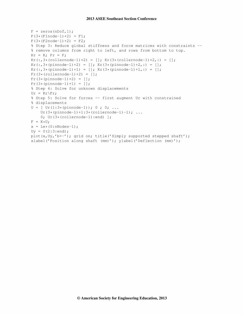
2013 ASEE Southeast Section Conference
F = zeros(nDof,1);F(3*(F1node-1)+2) = F1;F(3*(F2node-1)+2) = F2;% Step 3: Reduce global stiffness and force matrices with constraints --% remove columns from right to left, and rows from bottom to top.Kr = K; Fr = F;Kr(:,3*(rollernode-1)+2) = []; Kr(3*(rollernode-1)+2,:) = [];Kr(:,3*(pinnode-1)+2) = []; Kr(3*(pinnode-1)+2,:) = [];Kr(:,3*(pinnode-1)+1) = []; Kr(3*(pinnode-1)+1,:) = [];Fr(3*(rollernode-1)+2) = [];Fr(3*(pinnode-1)+2) = [];Fr(3*(pinnode-1)+1) = [];% Step 4: Solve for unknown displacementsUr = Kr\Fr;% Step 5: Solve for forces -- first augment Ur with constrained% displacementsU = [ Ur(1:3*(pinnode-1)); 0 ; 0; ...
Ur(3*(pinnode-1)+1:3*(rollernode-1)-1); ...0; Ur(3*(rollernode-1):end) ];
F = K*U;x = Le*(0:nNodes-1);Uy = U(2:3:end);plot(x,Uy,’b+-’); grid on; title(’Simply supported stepped shaft’);xlabel(’Position along shaft (mm)’); ylabel(’Deflection (mm)’);
© American Society for Engineering Education, 2013


![Analysis of Speed Reduction Assembly Output Shaft · 2020. 8. 16. · The static deflection of the shaft can be determined using Macaulay’s method [1] Fig 2: SFD and BMD 3.1Deflection](https://static.fdocuments.in/doc/165x107/613fd474b44ffa75b8047a18/analysis-of-speed-reduction-assembly-output-shaft-2020-8-16-the-static-deflection.jpg)