Shades of Brown and Green: Party E¤ects in ProportionalElection Systems �

Olle Folkey

IIES

November 12, 2009

Abstract

Small parties play an important role in proportional election systems. For example, theemergence and electoral success of environmental and anti-immigration parties have constitutedone of the central changes in the political landscape in Europe over the last three decades. Butwe do not know if this has actually had any implications for policy, since no methods existfor credibly estimating the e¤ect of legislative representation in proportional election systems.Because party representation is not randomly assigned, both observable and unobservable factorsin�uence policy outcomes as well as party representation. Using a part of the legislative seatallocation that is as good as random, I estimate the causal e¤ect of party representation onimmigration policy, environmental policy and tax policy in Swedish municipalities. The resultsshow that party representation has a large e¤ect on the �rst two policies, but not on the taxpolicy.

1. Introduction

A distinct feature of proportional election systems is the emergence and existence of small parties

(Duverger, 1954). Still, we do not know much about whether, and to what extent, individual

parties, small or large, shape policy. There are simply no suitable methods for estimating the e¤ect

of legislative representation of political parties in proportional election systems.1 In this paper, I

try to �ll this methodological gap and estimate how party representation a¤ects immigration policy,

environmental policy and tax policy.

To estimate the causal e¤ect of legislative representation, I use observations that are su¢ ciently

close to seat allocation thresholds, for part of the seat allocation to be considered as good as�The author gratefully acknowledges helpful comments from David Strömberg, Torsten Persson, Jim Snyder, Per

Pettersson-Lidbom, Ethan Kaplan, Donald Green, Matz Dahlberg, Orit Kedar, Emilia Simeonova, Albert Solé-Ollé,Jens Hainmueller, Peter Nilsson, Hans Grönqvist, Heléne Lundqvist, Erika Färnstrand Damsgaard, Erik Meyersson,Jon Fiva, Karin Edmark, Björn Tyrefors Hinnerich, and seminar participants at IIES, MIT, Harvard, CIFAR, Trond-heim NTNU, SULCIS, IEB Summer School, the 24th annual EEA congress, SLU and IFAU. The views expressed inthe paper are mine, as is the responsibility for any mistakes.

yIIES, Stockholm University, S-106 91 Stockholm, Sweden; folke@iies.su.se1 Around half of the democracies in the world, including most European countries, have political systems with

proportional representation, or elements of it.

random. The identifying assumption is that observations close to either side of a seat threshold

are equal in all respects, except party representation. If this holds, any observed di¤erences in

policy outcomes between observations on opposite sides of a seat threshold can be attributed to the

di¤erences in party representation. The identifying assumption is thus similar in spirit to that in

regression discontinuity design (RDD).2 Although the methodology is intuitively simple, there are

several complex methodical challenges associated with the inherent characteristics of proportional

election systems. This implies that I have to make several deviations, and developments, from

the typical RDD. Several of these methodological developments can be applied to other issues and

questions.

In addition to methodological advances, I also present a set of substantive results. Applying

the method to data from Swedish municipalities, I show that changes in legislative representation

have large and signi�cant e¤ects on immigration and environmental policy. However, I do not �nd

any evidence of legislative representation a¤ecting the municipal tax rate. The results also show

that OLS estimates of party representation e¤ects give misleading results.

Focusing on immigration and environmental policy is natural since the two policy areas seem

to have been central for the emergence of new small parties in Western Europe since the beginning

of the 1980�s. Examples of electorally successful anti-immigration parties include Front National

in France, Freiheitliche Partei Österreichs in Austria, Partij voor de Vrijheid in the Netherlands,

Dansk Folkeparti in Denmark and Vlaams Blok in Belgium. Green parties have been su¢ ciently

successful to gain parliamentary representation in several countries such as Germany, France, Italy,

Sweden and Belgium.

Proportionality of the election system has been central for the electoral success of green parties.3

To illustrate this, consider the United States and Germany, which both have strong environmental

movements. In Germany, where the representatives to the national parliament are elected pro-

portionally, the Greens (die Grünen) have been represented in the national parliament after every

election since 1983, commonly winning between 6 and 9 percent of the seats. Between 1998 and 2005

it was also part of the governing coalition. In the US, the Green Party has never been represented

in Congress, and only on a few occasions has it been represented in state legislatures. However,

the US environmental movement is still directly involved in policy formation through, for example,

lobbying and public campaigns.4 Thus, it is not clear whether the parliamentary representation of2 See Imbens & Lemieux (2008) for an overview of the RD methodology.3 Studies speci�cally focusing on the emergence and success of environmental parties include Kitschfelt (1989),

Rohrschneider (1993) and Burchell (2002).4 For example, the Sierra Club in the US has 1.3 million members.

2

German greens gives them a larger in�uence on public policy than US greens. This paper will help

me address the question of whether political representation actually gives environmental movements

better possibilities of in�uencing policy.

Proportionality of the electoral system has also been central for the emergence and electoral

success of anti-immigration parties.5 Even though it is unclear if, and how, representation of anti-

immigration parties has a¤ected policy, their electoral success is often met by strong public, and

political, reactions. An example of this is that the success of the German NPD, a party very far

to the right, with slogans like "Stop the Invasion by Poles", lead other parties to call for a ban of

NPD. For example, the Bavarian interior minister, Joachim Herrmann, stated that: "If we leave

the NPD to do what it wants until the federal republic is at risk, then we have missed the right

point for a ban". Given that we do not know how, or even if, representation of anti-immigration

parties a¤ects policy, it is unclear if the representation of parties like NPD politicians should be a

concern. This is another question this paper helps to address.

Apart from immigration and environmental policy, I also examine how legislative representation

a¤ects tax policy. The tax rate is a general-interest policy that, unlike immigration and environ-

mental policy, is basically de�ned on the left-right policy spectrum, which commonly de�nes how

governing coalitions are formed. This makes for an interesting comparison with the other two

policies and also allows me to relate the results to Petterson-Lidbom (2009) who, using an RDD,

estimates the e¤ect of legislative seat majorities on economic outcomes in Swedish municipalities.

There are few clear theoretical predictions of whether, or how, party representation a¤ects policy

in proportional election systems. But the assumption that individual parties a¤ect policy is central

in many theoretical models. In models comparing proportional and majoritarian representational

systems, the predicted di¤erences often rest on the assumption that individual parties, representing

minorities or special interests, shape policy outcomes; see for example Persson et al. (2007).

Similarly, the literature on the emergence of new parties over new policy issues, often taking its

starting point in Lipset and Rokkan (1967), frequently rests on the implicit assumption that the

legislative representation of a party will a¤ect policy. This is not obvious, however. Special-

interest parties, such as green parties and anti-immigration parties, are generally not part of the

traditional political establishment and seldom belong to governing coalitions. Furthermore, anti-

immigration parties often meet strong opposition in the public debate from parties taking an

opposite stance. From this perspective, estimating the e¤ect of legislative representation is essential5 For studies on the emergence and success of anti-immigration parties, see, for example, Jackman & Volpert

(1996), Golder (2003) and Rydgren (2005).

3

for understanding policy and party formation under proportional representation.

The scant knowledge about how party representation shapes policy outcomes is due to challeng-

ing methodical problems. Clearly, we expect voter preferences and characteristics to a¤ect both

party representation and policy outcomes. Thus, a positive relationship between the representation

of a green party and stricter environmental regulation does not necessarily mean that the green

party has a causal e¤ect on policy. It might simply be the case that when voters have strong en-

vironmental preferences, and vote for a green party, all parties become more "green". Since only a

subset of covariates that could a¤ect both representation and policy outcomes is easily observable,

or measurable, it is not possible to credibly estimate the e¤ect of party representation by including

a wide set of control variables. A credible estimation requires some exogenous variation in party

representation. Since it is not possible to randomly assign party representation, the remaining

option is to try to �nd some part of the party representation that can be considered to be as good

as random.

A common solution to estimating the causal e¤ect of legislative outcomes has been to adopt

a regression discontinuity design (RDD). Common to all previous studies is that they rely on the

assumption that a majority of political power is assigned in a random function close to the threshold

for winning a majority of either the vote share or the seat share. Examples of such studies include

Lee et. al. (2004), Ferreira & Gyorko (2009), Pettersson-Lidbom (2009) and Warren (2008).

However, applying this approach to legislative representation in proportional election systems is

not possible, as individual parties are rarely close to holding a majority of neither the vote share

nor the seat share. This motivates the development of a new methodological framework, in which

identi�cation of causal e¤ects is based on being close to a threshold for a shift in the seat allocation

instead of the threshold for a majority change.

To test the e¤ect of legislative representation on immigration policy, environmental policy and

tax policy, I use almost 300 Swedish municipalities (local governments). This has several advan-

tages. Parties focusing on these policy areas have been electorally successful in Swedish municipal-

ities. Swedish municipalities also have large opportunities to politically in�uence all three policy

areas that I examine. Finally, the municipalities are homogeneous with respect to both the political

system and the institutional framework.

My results show that changes in legislative representation have large and signi�cant e¤ects

on immigration policy, measured as the number of actively admitted refugee immigrants. The

representation e¤ects closely correspond to how voters perceive the parties. New Democracy, a

4

party which had a clear and strong anti-immigration position, also has the largest negative e¤ect

on immigration policy, while the party with the strongest pro-immigration position, the Liberal

Party, has the largest positive e¤ect. A one-percentage-point shift in seat shares between these two

parties would lead to the average municipality, which has a population of 30 000, actively admitting

ten more, or less, refugee immigrants per year during a four-year election period.

The results for environmental policy, measured through a survey-based environmental policy

ranking, also show large and statistically signi�cant e¤ects of changes in legislative representation.

The Environmental Party, with the strongest green pro�le in Sweden, has a large positive e¤ect

on the ambition level of municipalities� environmental policies. As in the case of immigration

policy, the estimated e¤ects of the other parties also correspond to how voters perceive the parties.

The estimated e¤ects suggest that an increase in the seat share of the Environmental Party of

�ve percentage points, at the expense of most other parties, could make a municipality undertake

environmental initiatives such as buying "green" energy or carrying out environmental information

campaigns.

The results for tax policy, measured through the municipal tax rate, also follow the voter

perceptions of the parties. The estimated e¤ects are too imprecise to be statistically signi�cant,

however. Pettersson-Lidbom (2009) �nds a large signi�cant e¤ect on the tax rate from left-wing

parties holding a seat majority, which suggests that legislative majorities, and not individual party

representation, constitute the relevant dimension for primary left-to-right policies such as the tax

rate.

Several mechanisms might potentially explain the representation e¤ects that I uncover. Party

representation could a¤ect what, and how, coalitions are formed; see for example Austen-Smith

& Banks (1988). The degree of representation could also be decisive for the voting power of a

party; see, for example, Banzhaf (1964) and Holler (1982). The legislative presence of a party could

a¤ect what, and how policies, are discussed in the legislature. Out of these mechanisms, I can only

examine the third. My results show that legislative presence cannot explain the representation

e¤ects.

Section 2 of the paper describes the identi�cation strategy, while Section 3 describes the data

and de�nes the parties�policy positions. Section 4 presents the results of the baseline speci�cation.

Section 5 shows results of alternative speci�cations and provides tests of the identifying assumption.

Section 6 covers some extensions to the baseline speci�cation and discusses the mechanisms behind

the results. Finally, Section 7 discusses the �ndings and concludes the paper.

5

2. Identi�cation Strategy

In this section, I �rst describe in detail why it is di¢ cult to estimate the policy e¤ects of party

representation in legislatures. Then, I propose a solution to this problem that involves comparing

outcomes in close elections.

Let me introduce some notation that is used throughout the paper. There are P parties indexed

by p = f1; 2; 3; :::; Pg. The number of votes for party p is denoted vp, and the total number of votes

is V =PP1 vp. The vector VP = (v1; v2; v3; :::; vP ) contains the votes for all parties. Analogously,

the number of seats of party p is denoted esp, and the total number of seats is S =PP1 esp. The seat

share of party p is denoted sp =espS ; and SP = (s1; s2; s3; :::; sP ) is a vector of the seat shares of all

parties.

For simplicity, I use three parties in all models and examples in this section. This is the simplest

setting that captures the speci�c characteristics of proportional election systems. Extending the

models and examples to more than three parties is straightforward and does not require any changes

in the model.

Given an allocation of votes, seats are allocated by the function esp = f (VP ; S) based on,

for example, the Sainte-Laguë or the d�Hondt method. A detailed description of seat allocation

methods in proportional election systems and how to adopt the method developed in this paper to

di¤erent seat allocation methods can be found in the Appendix.

2.1. Identi�cation problem

I wish to estimate the e¤ect of party representation, de�ned as the seat shares, SP , of parties,

on some policy, y, in municipality i. Let us assume that I wish to estimate the e¤ect of party

representation with a linear model:

yi = �+ �1s1i + �2s2i + "i: (2.1)

In this speci�cation with three parties, Party 3, p = 3, is omitted and used as the reference case.

Thus, what I estimate are the e¤ects of Party 1 or Party 2 when their representation increases at

the expense of Party 3.

The identi�cation problem arises because party representation is likely to be correlated with

the error term because voter preferences may directly a¤ect policy, "i = k (VP )+ui, where k (VP )

is an unknown function of the vote shares of the parties. Inserting this error term into the above

6

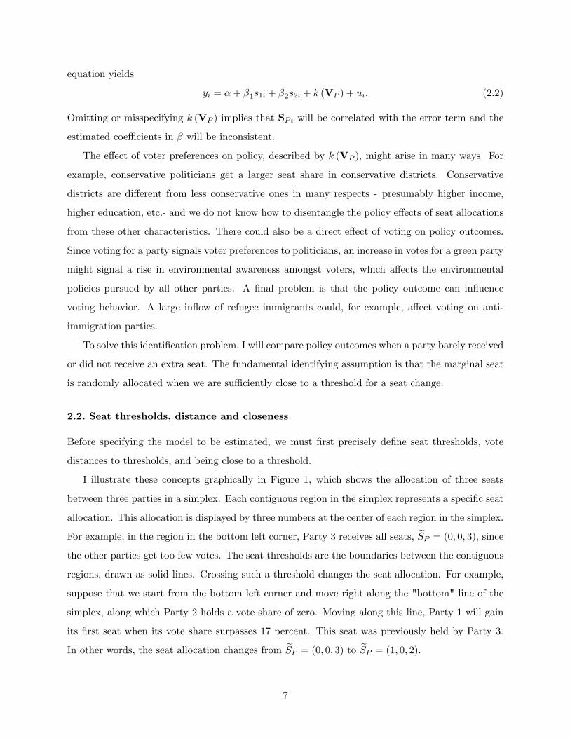
equation yields

yi = �+ �1s1i + �2s2i + k (VP ) + ui: (2.2)

Omitting or misspecifying k (VP ) implies that SPi will be correlated with the error term and the

estimated coe¢ cients in � will be inconsistent.

The e¤ect of voter preferences on policy, described by k (VP ), might arise in many ways. For

example, conservative politicians get a larger seat share in conservative districts. Conservative

districts are di¤erent from less conservative ones in many respects - presumably higher income,

higher education, etc.- and we do not know how to disentangle the policy e¤ects of seat allocations

from these other characteristics. There could also be a direct e¤ect of voting on policy outcomes.

Since voting for a party signals voter preferences to politicians, an increase in votes for a green party

might signal a rise in environmental awareness amongst voters, which a¤ects the environmental

policies pursued by all other parties. A �nal problem is that the policy outcome can in�uence

voting behavior. A large in�ow of refugee immigrants could, for example, a¤ect voting on anti-

immigration parties.

To solve this identi�cation problem, I will compare policy outcomes when a party barely received

or did not receive an extra seat. The fundamental identifying assumption is that the marginal seat

is randomly allocated when we are su¢ ciently close to a threshold for a seat change.

2.2. Seat thresholds, distance and closeness

Before specifying the model to be estimated, we must �rst precisely de�ne seat thresholds, vote

distances to thresholds, and being close to a threshold.

I illustrate these concepts graphically in Figure 1, which shows the allocation of three seats

between three parties in a simplex. Each contiguous region in the simplex represents a speci�c seat

allocation. This allocation is displayed by three numbers at the center of each region in the simplex.

For example, in the region in the bottom left corner, Party 3 receives all seats, eSP = (0; 0; 3), sincethe other parties get too few votes. The seat thresholds are the boundaries between the contiguous

regions, drawn as solid lines. Crossing such a threshold changes the seat allocation. For example,

suppose that we start from the bottom left corner and move right along the "bottom" line of the

simplex, along which Party 2 holds a vote share of zero. Moving along this line, Party 1 will gain

its �rst seat when its vote share surpasses 17 percent. This seat was previously held by Party 3.

In other words, the seat allocation changes from eSP = (0; 0; 3) to eSP = (1; 0; 2).7

Note that the number of seats of a party is a¤ected by the votes of all parties. Consequently,

the distance to a seat change cannot be measured only using the vote share of an individual party.

For example, the vote share at which Party 1 will receive its �rst seat depends on how the remaining

votes are distributed across Party 2 and Party 3. This implies that Party 1 may experience a seat

change while keeping its vote share constant.

I de�ne the distance between two vote vectors, V0P and V

1P , as the sum across parties of the

absolute vote di¤erences, measured in vote shares. That is, the distance between V0P and V

1P is

d�V0P ;V

1P

�=

p=PXp=1

��v1p � v0p�� : (2.3)

I then de�ne the minimal distance to a seat change for party p: Suppose that the election

outcome is V0P ; and the associated seat allocation to party p is s

0p = f

�V0P ; S

�: The minimal

distance to a seat change for party p is the minimal distance, d�V0P ;V

1P

�; to any point V 1P at

which the seat allocation for party p is di¤erent than at V0P , fp

�V0P ; S

�6= fp

�V1P ; S

�:

I will de�ne observations as being close to a threshold if the minimal distance to seat change is

less than a cuto¤ point, denoted by �. In Figure 1, close elections for party 1 (de�ned by � = 5

percentage points) are marked in grey. The large �ve percent value is chosen for illustrative reasons.

I use the much smaller � = 0:25 percentage points of the vote share in most empirical speci�cations.

In practice, measuring the minimal distance to a seat change is somewhat complicated. A

precise description of this can be found in the Appendix where I also provide a practical example.

2.3. Speci�cation

I now return to the speci�cation of the model to be estimated, which will compare outcomes in

elections where a party has barely received an extra seat to elections where it has barely not.

To implement this speci�cation, I need two indicator variables. One variable indicates all

observations where a party is close to a threshold. The other variable indicates whether the party

is close to and above or below such a threshold. This is the treatment variable. Formally, I de�ne

binary indicator variables for each party, cp, which takes the value of 12 for all observations where

the party is within distance � from a threshold, that is, for observations close to a threshold.6 I

also de�ne the treatment variables tp; which equal �12 if party p is close to and below a threshold,

6 The choice of � is a trade-o¤ between precision and internal validity. Decreasing � reduces the number ofidentifying observations, thus reducing the precision of the estimated e¤ects. The bene�t is that decreasing � increasesthe certainty that the identifying assumption holds. There is no formal rule for choosing � in this setting, makingthe choice of � a call of judgement.

8

12 if p is close to and above a threshold, and zero otherwise. Figure 1 illustrates the values of these

variables. The grey shading indicates close elections for Party 1 (c1 = 12). The horizontal stripes

indicate that Party 1 is just above a threshold (t1 = 12), and the vertical stripes indicate that Party

1 is just below (t1 = �12). I normalize this by assuming that the e¤ect of an additional seat depends

on the total number of seats in the legislature and thus, I divide the treatment and control variables

by this number.

The speci�cations I investigate are of the form

yi = �+ 1c1iSi+ 2

c2iSi+ �1

t1iSi+ �2

t2iSi+ g (VPi) + "i; (2.4)

where g (VPi) is a function of the vote shares of all parties. This speci�cation compares outcomes

when parties are just below or just above a threshold to receive more seats. The fundamental

identifying assumption is that within this range, it is essentially random whether a party receives

a seat, implying that corr( t1iSi ; "i) = corr( t2iSi ; "i) = 0.7 Since only observations close to the seat

thresholds are used for identi�cation, the control function, g (VPi), is only needed to reduce residual

variation, not to get consistent estimates.

Note that the e¤ect of a certain party gaining or losing a seat depends on what other party

is on the other side of the threshold. The e¤ect on taxes of a centrist party gaining a seat could

have a di¤erent e¤ect if it gains the seat at the expense of a right-wing party or a left-wing party.

In one case, the e¤ect is �centrist � �right�wing; in the other the e¤ect is �centrist � �left�wing: By

simultaneously estimating the e¤ect of all parties, this possibility is taken care of.8

I �nally discuss issues created by multiple election districts within a legislature. In this case,

e¤ects from multiple districts must be aggregated. This is done by aggregating the treatment

variable, tp, the control variable, cp, and the vote shares VPi, over all districts, N , using the

following speci�cation

yi = �+ 1c01iSi+ 2

c02iSi+ �1

1

Si

e=NXe=1

t1ie + �21

Si

e=NXe=1

t2ie + g�V0Pi

�+ "i: (2.5)

The control variable, c�pi, is now de�ned as the absolute value of the aggregated treatment variable:

c�pi = abs

e=NXe=1

tpie

!: (2.6)

7 Note that cov( t1iSi; "i) = E

h�t1i � t1i

� �1Si� 1

Si

�"ii

= EhE��t1i � t1i

�"i j Si

� �1Si� 1

Si

�i= 0 if

E��t1i � t1i

�"i j Si

�= 0; that is if the treatment is uncorrelated with "i for all legislature sizes, Si.

8 An alternative approach would be to separately estimate the e¤ect of crossing a seat threshold between each pairof parties. However, in the case of this paper, it would, give the same results as estimating the e¤ect of all partiessimultaneously.

9

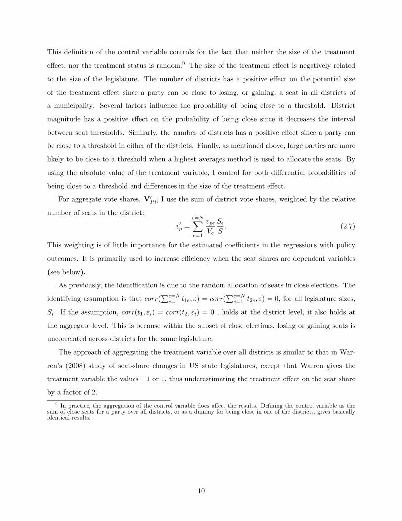
This de�nition of the control variable controls for the fact that neither the size of the treatment

e¤ect, nor the treatment status is random.9 The size of the treatment e¤ect is negatively related

to the size of the legislature. The number of districts has a positive e¤ect on the potential size

of the treatment e¤ect since a party can be close to losing, or gaining, a seat in all districts of

a municipality. Several factors in�uence the probability of being close to a threshold. District

magnitude has a positive e¤ect on the probability of being close since it decreases the interval

between seat thresholds. Similarly, the number of districts has a positive e¤ect since a party can

be close to a threshold in either of the districts. Finally, as mentioned above, large parties are more

likely to be close to a threshold when a highest averages method is used to allocate the seats. By

using the absolute value of the treatment variable, I control for both di¤erential probabilities of

being close to a threshold and di¤erences in the size of the treatment e¤ect.

For aggregate vote shares, V0Pi; I use the sum of district vote shares, weighted by the relative

number of seats in the district:

v0p =e=NXe=1

vpeVe

SeS: (2.7)

This weighting is of little importance for the estimated coe¢ cients in the regressions with policy

outcomes. It is primarily used to increase e¢ ciency when the seat shares are dependent variables

(see below).

As previously, the identi�cation is due to the random allocation of seats in close elections. The

identifying assumption is that corr(Pe=Ne=1 t1e; ") = corr(

Pe=Ne=1 t2e; ") = 0, for all legislature sizes,

Si. If the assumption, corr(t1; "i) = corr(t2; "i) = 0 , holds at the district level, it also holds at

the aggregate level. This is because within the subset of close elections, losing or gaining seats is

uncorrelated across districts for the same legislature.

The approach of aggregating the treatment variable over all districts is similar to that in War-

ren�s (2008) study of seat-share changes in US state legislatures, except that Warren gives the

treatment variable the values �1 or 1, thus underestimating the treatment e¤ect on the seat share

by a factor of 2.

9 In practice, the aggregation of the control variable does a¤ect the results. De�ning the control variable as thesum of close seats for a party over all districts, or as a dummy for being close in one of the districts, gives basicallyidentical results.

10

3. Data Description

In this section of the paper, I provide background information on Swedish municipalities, including

the most important institutional features of the political system. I also describe outcome variables

and political parties. Finally, I show what importance the parties attach to the three examined

policy dimensions and how they position themselves on them.

3.1. Political Institutions of Swedish Municipalities

Swedish politics take place at three geographical levels: the national, the county, with 20 counties,

and the municipal, with 290 municipalities. Municipalities di¤er widely in land area, from 9 to

19 447 square kilometers, and population, from 2 558 to 780 817 inhabitants. The municipalities

have a large freedom in organizing their activities. They have the right to levy income taxes, which

account for roughly two thirds of municipal government income. Day care, education and the care

of elderly and disabled are the most important expenditure posts. Expenditures are, on average,

around 20 percent of GDP.

The municipalities are governed by elected councils. The councils appoint subcommittees that

are responsible for di¤erent policy areas such as education and city planning. The municipalities

have a "quasi parliamentary" system where the heads of the subcommittees are appointed by the

governing majority, which is the equivalent of the government at the national level. However,

coalitional discipline is not binding, such that parties of the governing majority are not required to

vote together on all policy issues. This implies that alternative coalitions can be formed on speci�c

policy areas and issues.

Elections to the municipal councils are held every fourth year (before 1994 every third year).

The members of the governing councils are elected from multimember electoral districts. Around

two thirds of the municipalities only have one electoral district, but the large municipalities have

multiple districts. The election law dictates that a municipality with more than 24 000 eligible

voters, or a legislative council with more than 50 seats, must have at least two electoral districts.

When a municipality has more than one district, representatives are elected separately from each

district.

Within each district, the modi�ed Sainte-Laguë method is used to distribute the seats.10 The

number of seats per district is legally bound between 15 and 49. Unlike the national level, no seats

10 The decision to use the modi�ed Sainte-Laguë method in Sweden, taken in 1952, was supposedly made to givethe Communist Party a disadvantage in the seat allocation to Swedish Parliament (Grofman & Lijphart, 2002).

11

are used to "even out" di¤erences between the share of votes and seats caused the allocation of

votes between the districts. There is no explicit electoral threshold for gaining representation in

the municipal council.11

3.2. Outcome Variables

I will look at three policy outcomes in the municipalities: immigration policy, environmental policy

and the tax rate. Descriptive statistics for the three outcome variables are provided in Table 1. In

the estimations, each policy outcome is measured as an average over the relevant election period.

Swedish Municipalities have large possibilities of in�uencing the in�ow of immigrants. Once

refugee immigrants have been granted asylum in Sweden, they are placed in municipalities through

the placement program of the Swedish Immigration Agency. The process of this national program

has, in principle, remained the same from 1985 until today (Emilsson, 2008). The most important

change was that refugee immigrants were able to opt out of the placement program after 1994.

Each municipality must still be able to decide how many refugee immigrants should be received

through the program. Importantly, there have been large annual variations in the in�ow of refugee

immigrants to Sweden. For example, the intake spiked in 1994 and 2006 due to the wars in former

Yugoslavia and Iraq.

As the outcome variable for immigration policy, I will use the number of refugee immigrants

per capita placed in the municipality through the national placement program. The number placed

in each municipality is negotiated between the immigration agency and the municipalities. The

in�ow through the placement program is relatively large, see Table 1, with an annual average of 1.9

immigrants per 1000 inhabitants, or 58.6 immigrants in absolute terms. Moreover, immigration is

often a highly contentious issue in municipal politics, sometimes even leading to the formation of

new local parties. The distribution of placed refugee immigrants per capita between municipalities

is skewed to the right. For this reason, I use a logarithmic transformation in the estimation.

When it comes to environmental policy, the municipalities have numerous responsibilities and

freedoms. Their responsibilities include wastewater treatment, waste collection, zoning, building

permits, giving permissions for, and controlling, smaller and medium sized industries. In each of

these areas, the municipalities also have large freedoms in deciding and carrying out their own

policies.12

11 Naturally, there is an implicit electoral threshold that is determined by the number of seats in each district. Thelarge variation in seats among the districts gives a large variation in the implicit threshold, ranging from around 1.5to 5 %.12 I add one immigrant to all municipalities to be able to include all observations in the estimations. Excluding

12

As the outcome variable for environmental policy, I will use an environmental ranking of all

Swedish municipalities made by a Swedish environmental magazine (Miljö Eko, 1993-2001) in every

year between 1993 and 2001. This measure has previously been used by Dahlberg & Mörk (2002)

and Forslund et. al. (2008). The ranking is based on the initiatives undertaken by the municipality

and not the environmental outcomes. Thus, it is more appropriate to consider the environmental

ranking as an approximation, rather than as an absolute measure of the environmental policy

performance. The indicators used in the ranking include measures of sustainable procurement,

recycling programs, doing environmental audits, and "green" information to the inhabitants. The

contents and the maximum score of the survey changed somewhat over the years. For this reason,

I use the municipal score relative to the maximal score in the estimation.

The municipalities are free to set the tax rate as they see �t, as long as the budget de�cit is not

too large.13 The tax rates vary considerably between municipalities, which can be seen in Table 1.

They also vary considerably over time, with a large increase between 1991 and 1992 caused by a

shift in responsibility for the care of the elderly from counties to municipalities. Tax rate expressed

as a percentage is used as the outcome variable.

3.3. Parties, Policy Position and Importance

Currently, there are seven parties in Swedish parliament and those parties also dominate municipal

politics, although many municipal councils also have representatives from local parties. The parties

are traditionally divided into two blocks with the Social Democrats and the Left Party in the left

block and the Conservative Party, the Center Party, the Liberal Party and the Christian Democrats

in the right block. At the municipal level, the formation of governing coalitions does not always

follow this division. For example, it is common that the parties from the middle of the left-right

political spectrum form governing coalitions. The Environmental Party can either be classi�ed as

belonging to the left block, as in Svaleryd & Vlachos (2009) for example, or as independent, as in

Pettersson-Lidbom (2008) for example. While the Environmental Party nowadays sides with the

left block in national politics, the picture is more subtle in municipal politics. Data on governing

coalitions from the elections in 1994, 1998 and 2002 suggest that it is appropriate to classify the

Environmental Party as block independent in municipal politics.

Apart from the seven national parties, the populist New Democracy had a successful election

observations with no immigrants does not change the results, nor does using alternative transformations.13 In the election period between 1991 and 1993, the municipalities were not allowed to raise taxes. The results

are only marginally a¤ected by excluding this election period from the estimations.

13

in 1991, when it won 6.7 percent of the votes in the parliamentary elections and 2.8 percent in the

municipal elections. Even though the party collapsed at the national level in 1994, it maintained

seats in 37 municipal councils before it more or less vanished from Swedish politics in the election

of 1998. New Democracy had four core issues: to reduce immigration, reduce taxation, make the

public sector more e¢ cient and "politics should be fun" (Rydgren, 2002).

Descriptive statistics for the parties are provided in Table 2, along with notation14 and how the

voter perceived policy position and importance. The size of each party is illustrated in Figures 2

and 3, where the seat share and the seat distribution for each party is shown in a histogram. Both

seat shares and seats for the three largest parties, the Social Democrats, the Conservative Party

and the Center Party, vary considerably across municipalities. Still, it is only the Social Democrats

that frequently hold a majority of the seats. The other parties rarely hold more than ten percent

of the seat share, or more than �ve seats.

To form a prior on how parties might a¤ect policy, it is vital to know both what policy areas

are important for each party and the party positions in these areas. There are no studies that have

quanti�ed the importance attached by Swedish parties to speci�c policy areas. While there is an

extensive literature on the positions of Swedish parties in the left-right policy space,15 there are

no studies that have quantitatively measured their positions on immigration and environmental

policies. Consequently, I construct my own measures of these features using survey data from

the Swedish National Election Studies Program (Statistics Sweden, 1982-2002).16 The results are

presented in Table 2 and Figure 5.

To measure policy importance, I use a set of questions where the respondents list the �ve most

important policy issues for each party. My index of importance of policy area y for party p is the

share of respondents that have listed an issue in policy area y as important for party p. These

questions are part of the survey in every election, which means that I can use data from every

election period17 covered by data on the outcome variables.

To measure policy positions, I take the commonly used approach of measuring how voters, on

average, place the parties on pre-constructed policy scales.18 I use a set of questions where the

respondents place each party on a policy scale, from 1 to 10, in various policy areas. For immigration

14 All election data have been collected from Statistics Sweden.15 Gilljam & Oscarsson (1996), for example.16 The studies are survey based and have been carried out by the Department of Political Science at Göteborg

University and Statistics Sweden in conjunction with each election since 1950. Each study has about 4000 respondents.17 New Democracy was only included in 1991 and 1994. The Environmental Party is included in the survey from

1988 and onward. The Christian Democrats were not included in 1982 and 1988.18 Used in Macdonald et. al. (1991), Westholm (1997) and Kedar (2005), for example.

14

policy, parties were positioned according to their preferences for admitting more refugee immigrants,

with the score of 10 being most pro-immigration. For environmental policy, the parties were

positioned on a "green scale", with 10 as the score for being the most green. There is no explicit

question in the election survey where the parties are positioned on taxes. Instead, I use the parties�

position on the left-right scale as a proxy for their position on taxes. Questions on environmental

policy and immigration policy were only included in the 1994 election, so I can only use that survey.

Figure 5 illustrates the measures for each respective policy area. In the �gure, the perceived

policy positions are illustrated by the parties�position on the horizontal axis, while the perceived

policy importance is illustrated by the size of the markers.

New Democracy is, by far, most anti-immigration and also the party for which immigration

is most important. On the other side of the policy spectrum, the Liberal Party is most pro-

immigration and gives the second highest importance to immigration policy. This is consistent with

Green-Pedersen & Krogstrup (2008) who argue that New Democracy and the Liberal Party are the

only two parties with wide-spread support that brought up immigration policy as a central policy

issue in Sweden during the period studied in this paper. New Democracy used limiting immigration

as one of its core election issues, while the Liberal Party was the only party to properly engage

in a debate against New Democracy about immigration. This was something manifested in public

by the former leader of the Swedish Liberal Party, Bengt Westerberg, who after the Center-Right

victory in the election of 1991, refused to appear on TV with the leaders of New Democracy. This

was met by New Democracy�s leader Bert Karlsson wishing Westerberg�s daughter to be given

AIDS by an African immigrant.

Figure 5 also shows that the Environmental Party has the most "green" policy position and

gives environmental policy the highest importance. The Center Party also stands out from the other

parties both in "greenness" and high policy importance, even though this importance was greater

before the Environmental Party gained widespread support. There is no party on the opposite side

of the green scale that also placed importance on environmental policy.

The positions on the left-right policy scale, also illustrated in Figure 5, follow the division of

the blocks. The Left Party and the Conservative Party take opposite positions at the extremes of

the scale and are also the parties placing most importance on taxes. The positions are basically

the same as in Gilljam & Oscarsson (1996).

15

4. Baseline Speci�cations

In this section, I �rst estimate the e¤ect of the treatment variable, tp, on the seat share of each

party in the legislature. To see if the seat shares in�uence policy, I then use the treatment variable

to estimate the e¤ect on policy outcomes.

4.1. Results for seat shares

I start with a graphical analysis of the average e¤ect of a party moving over a seat threshold on

a party�s seat share at the electoral-district level.19 I then regress the treatment variable, tp, on

seat share at the municipal level. Data from all elections between 1982 and 2002 are used in the

analysis.

The graphical analysis follows the standard RD design procedure. I plot the binned averages

of party seat shares against the distance to a seat change, using a bin bandwidth of 0.1%. To

investigate whether the treatment e¤ect is a¤ected by the size of the party, I split the sample into

two groups below and above the sample median of 7.3 percentage points.

The results are displayed in Figure 4. The seat shares clearly jump at the thresholds. This jump

is less distinct for the larger parties, even though it is of the same magnitude in percentage points.

This is because there is a larger variation in the seat share for large parties and, most importantly,

a large party is often close to both winning and losing a seat. The size of the jump is almost three

percentage points. This is because the average district magnitude is 30, so winning one extra seat

means, on average, an increased seat share of 1/30.

Turning to the regression analysis, I regress the seat share of each party on treatment variable,

tp; controlling for being close to a threshold by cp. I use three de�nitions of close elections, with

cut-o¤ distances to a threshold of 0:5%; 0:25% and 0:1%. The model is estimated both with and

without a fourth-order polynomial of the vote share, v0p.20

The results in Table 3 show a clear e¤ect of the treatment variable, tp, on the seat share for all

parties. The e¤ect is always positive and often close to 1. Including the fourth-order polynomial

vote share control function greatly enhances the precision of the estimates, even though it does

not signi�cantly change their size. After controlling for vote shares, the e¤ect is always highly

signi�cant and close to 1, but decreases when observations further from the threshold are included

19 It is not possible to make a graphical analysis at the municipality level when municipalities have multiple electoraldistricts.20 Using another polynomial to de�ne g (v0Pi) a¤ects neither the size nor the precision of the estimates.

16

(� increased). The latter can also be seen in Figure 4, as the average di¤erence in seat shares above

and below the threshold decreases with the distance to the threshold.

Table 3 shows the number of identifying observations for each party (observations where tp 6= 0).

There are more identifying observations for the larger parties, since they have a higher probability

of being close to a threshold. The share of identifying observations is relatively large. In total,

there are about 2000 observations for the elections between 1982 and 2002. Out of these between

500 and 1000, depending on the size of the party, are identifying observations for � = 0:25%.

4.2. Results for policy

I now estimate the e¤ects of party representation on policy. When discussing the results, I focus

on parties with the largest expected in�uence on each policy area, which are those perceived as

having the most extreme policy positions and as giving high importance to the policy areas.

In the baseline speci�cation, corresponding to equation 5, I estimate the e¤ect of party repre-

sentation on policy outcomes in reduced form, using the treatment variable, tp. To de�ne closeness,

I use the cut-o¤ distance to a threshold of 0.25 percentage points of the vote share, � = 0:25%. The

control function of the vote share, g (V0Pi), is de�ned as a fourth-order polynomial. I also include

election-period and municipality �xed e¤ects. The Social Democrats, S, is used as the reference

(omitted) party in this and all other speci�cations. That is, all estimated e¤ects on policy refer to

a seat share gain of party p at the expense of the Social Democrats: �p � �S .

To evaluate if there are any signi�cant party e¤ects, it is instructive to look at comparisons

between all pairs of parties. For example, regarding immigration policy, it is natural to compare

what happens if New Democracy, ND, gains a seat from the Liberal party, FP , (�ND � �FP =

(�ND � �S)� (�FP � �S)), because these are the parties with the most extreme policy positions.

The estimation results are presented in Table 4. In Figures 6-8, I plot the point estimates for

each policy against the parties�policy positions, as perceived by the voters. The size of the markers

in these �gures is weighted by perceived importance of the policy area for each party. Finally,

Table 5 shows the cross-party comparisons (�p � �p00) together with p-values for the hypothesis

(�p 6= �p00) for the two parties that are perceived as giving most importance to the respective

policy areas. Table 4 also includes the results from OLS21 and 2SLS regressions. In the latter, the

treatment variable tp is used to instrument the e¤ect of seat shares on policy outcome.22

21 The OLS speci�cation is de�ned by equation 2.1 and includes election period and municipality �xed e¤ects.22 More speci�cally, I use equation 2.5 in the �rst stage to instrument the seat share of each party with the

treatment variable, tp. In the second stage, I once more use equation 2.5, but replace the treatment variables with

17

Immigration Policy The results for immigration policy are presented in Tables 4 and 5 and

Figure 6. What stands out in Column 1 of Table 4 is the large negative point estimate of New

Democracy. The Liberal Party has the largest positive point estimate. Recall that these are the

only national parties that have pro�led themselves on immigration policy and are perceived by

voters as having the most extreme policy positions. Figure 6 plots the estimated policy e¤ects

against the perceived policy positions and shows a striking correspondence between the perceived

policy positions and the estimated e¤ects of New Democracy and the Liberal Party. The �gure

also shows that the estimated e¤ects of the other parties are in line with voter perceptions.

Table 5 shows that the e¤ect of New Democracy is signi�cantly negative as compared to all seven

national parties. This can be seen in Column 1, which shows the e¤ect of New Democracy relative

to each individual party, speci�ed in the �rst column. Furthermore, the e¤ect of an increased seat

share for the pro-immigration Liberal Party is positive and signi�cant as compared to all parties

except the Environmental Party and the Social Democrats. This can be seen in Column 2. Note

that the coe¢ cients in the row for the Social Democrats are the same as the regression coe¢ cients

in Table 4, in which the Social Democrats are used as the reference party. That none of the

other parties signi�cantly a¤ects immigration is quite expected, given that they have not pro�led

themselves in this dimension of policy.

The estimated e¤ects are fairly large. The estimated di¤erence between New Democracy and

the other parties is between 11 and 22. A di¤erence of 10 between a pair of parties suggests that

the placement of refugee immigrants would change by ten percent due to a seat share shift of one

percentage point between the parties. This corresponds to a change of six placed refugee immigrants

per year in the average municipality.

To exemplify these e¤ects, I compare the placement of refugee immigrants after the election

in Oxelösund, in the county of Stockholm, in 1991 to the placement after the election in nearby

Nynäshamn in 1994. In these elections, New Democracy and the Liberal Party were close to (using

� = 0:25%), and on opposite sides of, seat thresholds. In Oxelösund, New Democracy received 7.82

percent of the votes and two seats (out of a legislature total of 31), while the Liberal Party received

7.92 percent of the votes and three seats. Obviously, with a vote share shift of 0.1 percentage points,

the seat allocation between the parties would have shifted. In Nynäshamn, New Democracy received

1.70 percent of the votes and one seat (out of a legislature total of 45), while the Liberal Party

received 5.52 percent of the votes and two seats. With a vote share shift of only 0.14 percentage

the �tted values of the seat shares from the �rst stage.

18

points, New Democracy could have been left without a seat and the Liberal Party would then have

gained a third seat. It turned out that Oxelösund placed an average of 69 refugee immigrants,

while Nynäshamn placed an average of 40. The estimated e¤ects suggest that about three quarters

of this di¤erence can be explained by the di¤erences in marginal seat share allocations for New

Democracy and the Liberal Party which are as good as random.

Simple OLS estimates of the e¤ect of seat shares on policy produce misleading results, as can

be seen in Column 2 of Table 4. OLS estimates suggest a negative and signi�cant e¤ect when the

Liberal Party wins seats from several other parties. Given that the estimated e¤ect of the treatment

variable on the seat share is close to one, the 2SLS estimation should provide results that are only

marginally di¤erent from the baseline speci�cation. This is indeed what I �nd in Column 3 of Table

4.

Environmental Policy I now move on to discuss the results for environmental policy, presented

in Tables 4 and 5 and Figure 7. The Environmental Party, the only party with a clear green pro�le,

has the largest positive point estimate in Column 4 of Table 4. The other party with a relatively

green image, the Center Party, has a point estimate that corresponds to the median e¤ect of all

parties. New Democracy, which is perceived as being the least "green", has the largest negative

point estimate, albeit with a large standard error. As in the case of immigration policy, Figure 7

shows a striking correspondence between the estimated e¤ects and the perceived policy positions.

The exception is the large positive point estimate for the Conservative Party, which is not consistent

with the voters perceiving the Conservative Party as one of the least "green" parties.

Column 3 of Table 5 shows that an increased seat share for the Environmental Party has a

positive and signi�cant e¤ect on environmental policy when the seats are taken from all parties

except the Conservative Party. The voters perceive the Center Party as second to the Environmental

Party in both "greenness" and the importance given to environmental policy. This party does not

have a positive signi�cant e¤ect vis à vis any party, as shown in Column 4. Not shown in the table

is the fact that the Conservative Party has a signi�cantly positive e¤ect as compared to several

parties. The negative e¤ect of New Democracy is, however, only signi�cant as compared to the

Environmental and the Conservative Party.

As in the case of immigration policy, the estimated e¤ects are large. The estimated di¤erence

between the Environmental Party and most other parties is around two. This implies that the

relative environmental ranking would change by two percentage points from a seat share shift of

19

one percentage point between the parties. That the policy e¤ect is relatively large is not surprising.

Some of the policies required to increase the environmental ranking are easily implemented. A shift

in the relative ranking by ten percentage points could, for example, be achieved by implementing

a information campaign to the citizens and companies of the municipality.

To exemplify the estimated e¤ects, I will compare the environmental rankings after the 1994

elections in the municipalities of Forshaga and Årjäng in the rural county of Värmland in Eastern

Sweden. In Forshaga, the Environmental Party received 3.69 percent of the votes and two seats

(out of a legislature total of 41), while in Årjäng it received 3.55 percent of the votes and one

seat (out of a legislature total of 41). In both elections, it would have been su¢ cient with a vote

share shift of less than 0.1 percentage points to change the seat allocation for the Environmental

Party. The seat share di¤erence between the two municipalities for the Environmental Party of 2.5

percentage points suggests that the environmental ranking would be �ve percent higher in Årjäng,

and �ve percent lower in Forshaga if the Environmental Party had ended up on the other side of

the seat threshold. The relative environmental ranking during the election period was 46 percent

for Forshaga and 35 percent for Årjäng. Half of this di¤erence (�ve percentage points) can thus be

explained by the di¤erence in seat share for the Environmental Party which is as good as random.

The estimated di¤erence also corresponds to the fact that in each year during the election period,

Forshaga performed better at providing environmental information to its citizens.

The OLS estimates in Column 6 of Table 4 fail to identify any e¤ect of the Environmental

Party, or any other party. This provides further evidence of the OLS providing misleading results.

As for immigration policy, the 2SLS speci�cation (Column 5 in Table 4) provides results that are

only marginally di¤erent from the baseline speci�cation.

Tax Rate The results for the tax rate are presented in Tables 4 and 5 and Figure 8. Column 7 of

Table 4 shows that the Conservative Party has the largest negative point estimate. This is indeed

the party that voters perceive as the right-most party on the left-right policy spectrum, and as the

party that gives the highest importance to tax policy. Even though the Left Party is furthest to

the left, it is not the party with the largest positive point estimate on tax policy. Figure 8 shows a

clear correspondence between the estimated e¤ects of the parties. The correspondence is not nearly

as striking as for the two previous policies, however.

When looking at cross-party comparisons, the standard errors are su¢ ciently large to eliminate

all signi�cant di¤erences between any pair of parties. This is shown for the Left Party and the

20

Conservative Party in Table 5. Even though the e¤ects are in line with voter perceptions, they are

not su¢ ciently large to compensate for the large standard errors.

The point estimates are actually quite large. The di¤erence in e¤ects between the Left Party

and the Conservative Party is three. This implies that a ten percentage point shift in seat shares

between the two parties would change the tax rate by 0.3 percentage points. This magnitude is in

line with the e¤ects found by Petterson-Lidbom (2008) from the traditional left-wing parties holding

a majority of the seats. Hence, I cannot really draw any �rm conclusion that party representation

does not have any e¤ect on the tax rate.

There are no substantial di¤erences between the baseline, 2SLS and OLS speci�cations (see

Columns 8 and 9 in Table 4).

5. Alternative Speci�cations and Robustness Checks

In this section, I evaluate the validity of the identifying assumption by testing alternatives to the

baseline speci�cation and conducting several robustness checks.

5.1. Alternative Speci�cations

Are the estimated e¤ects of party representation on policy sensitive to using alternative speci�ca-

tions? To corner this question, I will test speci�cations with di¤erent cut-o¤ values to de�ne close

elections, �, and speci�cations with alternative sets of covariates. I start by de�ning the alternative

speci�cations. Then, I discuss the general �ndings for each alternative speci�cation. Finally, I

discuss results that are speci�c to each policy outcome.

In Tables 6, 7 and 8, I investigate eight alternative speci�cations for each policy outcome. I test

two alternative cut-o¤ values to de�ne close elections, � = 0:5%, in Columns 1-2 of each table, and

� = 0:1%, in Columns 8-9 of each table. For each of the two cut-o¤ values, I use speci�cations both

with and without municipality �xed e¤ects. Using the cut-o¤ value from the baseline speci�cation,

� = 0:25%, I examine four alternative speci�cations. In the �rst speci�cation (Column 3), I do not

include any control variables. I then add the vote share control function (Column 4) and election

period �xed e¤ects (see Column 5). As a point of reference, I show the results of the baseline

speci�cation, which includes municipality �xed e¤ects (Column 6). Finally, I add a vector of control

variables23, including education level, demographic composition and population size (Column 7).

23 Data for the control variables are collected from Statistics Sweden.

21

As for the cut-o¤ points for de�ning close elections, �, the standard errors decrease when �

increases. This is intuitive, since the number of identifying observations increases as � increases.

Changing the interval also changes the point estimates, even though no changes are statistically

signi�cant. The coe¢ cients change has two explanations. A higher value of � expands the sample

of identifying observations and eventually makes the treatment endogenous. Using � = 0:5%,

the di¤erence in the vote share for a small party on opposite sides of the "close interval" is not

arbitrary, implying that the interval might be too wide. The results are also more sensitive to

including municipality �xed e¤ects for � = 0:5% than for the two smaller intervals. The results

suggest that � = 0:5% is too wide a de�nition of close elections, while the large standard errors

make � = 0:1% too narrow a de�nition.

If the identifying assumption holds, the covariates should only a¤ect the standard errors and

not the point estimates. This is indeed the case. The most important reduction in standard errors

is achieved by including election-period �xed e¤ects; see the di¤erence between Columns 4 and

5. There is also a fairly large reduction in standard errors from including the vote share control

function g (V0Pi), compare Columns 3 and 4, and municipality �xed e¤ects, compare Columns 1 and

2, Columns 5 and 6, and Columns 8 and 9. Including the vector of control variables has minimal

e¤ects on both the point estimates and the standard errors, as seen in Columns 6 and 7.

I now discuss the speci�c results for each policy area, starting with immigration policy. The

main results, shown in Table 6, are not sensitive to the alternative speci�cations. The reduction in

standard errors, obtained by including the covariates, is important for getting statistically signi�cant

results, however.

The alternative speci�cations for environmental policy in Table 7 show that the positive esti-

mated e¤ect of the Environmental Party, MP , is not very sensitive. When using � = 0:5%, the

point estimate decreases, but the e¤ect is still signi�cant as compared to several other parties. For

the Conservative Party, M , the positive estimated e¤ect is more sensitive both to changing the

de�nition of close elections and using di¤erent sets of covariates.

The results of the alternative speci�cations for the tax rate are shown in Table 8. Here, the

reduction in standard errors when including covariates is much larger than for the two other policies.

The large reduction when including municipality �xed e¤ects is likely to be caused by long-term

di¤erences in economic conditions between municipalities. Even though the point estimates are

sensitive to using alternative speci�cations, none of the alternative speci�cations indicate that

representation of individual parties a¤ects the tax rate.

22

5.2. Robustness Checks

To check the validity of the identifying assumption, I take two approaches. I graphically examine

if there is a shift in the vote share when moving over a seat threshold. I also regress the treatment

variable, tp, on municipal background characteristics that should not be a¤ected by political factors

in the short run.

First, I graph the balancing of vote shares close to seat thresholds. Since the distance to a seat

threshold is not only dependent on the vote share of the individual party, this analysis is important

to validate that the distance measure is correctly de�ned. A shift in the vote share when moving

over a threshold would indicate an invalid distance measure and a biased treatment variable.

In the graphs, I plot the vote share, instead of the seat share, against the distance to a seat

threshold. As before, I use binned averages with a width of 0.1%. To investigate whether the

identifying assumption holds irrespective of party size, I split the sample into two groups, below

and above the sample median of 7.3 percentage points. Figure 9 clearly shows that there is no

"jump" in the vote share at the seat threshold, irrespective of party size. This suggests that the

identifying assumption holds.

In the regression analysis, I test if the treatment variable, tp; has an e¤ect on background

variables that should not be a¤ected by short-term political outcomes. A signi�cant outcome

would indicate an invalid identifying assumption. The background variables I examine are real

income per capita, population share with higher education, population share of children and the

municipal population in logarithmic form. The vector of control variables is not included since

some of the control variables are now used as outcome variables. I estimate the model both with

and without municipality �xed e¤ects.

The results are presented in Table 9. Some of the parties are found to have signi�cant e¤ects

on the background variables in comparison to other parties; see, for example, the Environmental

Party, MP , in Column 1, the Center Party, C, in Columns 2 and 8, and the Conservative Party,

M , in Column 8. Unlike the estimates for the e¤ects on policy outcomes, however, these estimates

are very sensitive and disappear when municipality �xed e¤ects are included or excluded. This

suggests that the signi�cant e¤ects are random �ndings. Thus, the results do not provide any

evidence against the identifying assumption.

23

6. Mechanisms of representation

The results in the baseline speci�cation clearly show that party representation a¤ects policy out-

comes. But the results provide little guidance regarding the mechanisms behind the representation

e¤ects. In this section, I will carefully test one of the potential mechanisms, which is legislative

representation. Then, I discuss other potential mechanisms.

6.1. Legislative Representation

The methodology of this paper allows me to examine if legislative presence is an important mech-

anism behind the estimated representation e¤ects. Such a mechanism could re�ect the presence of

a party a¤ecting the salience of a given policy area in the legislature. For example, having a green

party in the legislature might raise the awareness of environmental issues amongst all parties. If

legislative presence is an important mechanism, we would expect representation e¤ects to be larger

for the �rst seat won by the party.

To estimate if the representation e¤ect is larger for the �rst seat, I add a second treatment

variable to the baseline speci�cation, de�ned by equation 2.5. I de�ne the second treatment variable

as an interaction term between the representation treatment variable, 1Si

Pe=Ne=1 tpe, and a dummy

for being close to the threshold for the �rst seat, crp. In practice, this means that I estimate the

representation e¤ect conditional on being close to the threshold for the �rst seat. As previously,

being close to a threshold is de�ned by the cut-o¤ value �. In the estimations, I use the same

de�nition of close elections, � = 0:25%, as in the baseline speci�cation. Since it is not random if

the party is close to the threshold for the �rst seat, I also include, crp, as a control variable. The

results are presented in Table 10. The estimates for the linear representation e¤ects are presented in

the rows labeled Seat Share, while the representation e¤ect for gaining the �rst seat are presented in

the rows labeled First Seat. I also show the share of the identifying observations for each treatment

variable.

In general, the results suggest that none of the key �ndings from the baseline speci�cation can

be explained by legislative presence. For some parties and policies, the representation e¤ects are

actually larger when the party is not close to the threshold for the �rst seat. This suggests that there

could be some type of increasing returns to scale for small parties in�uence on policy. Explanations

for this include that representatives can argue more forcefully when having the support of fellow

party members, or that very small parties are very likely to be dummy players in forming coalitional

24

majorities.24

The results for immigration, shown in Column 1 of Table 10, suggest that the representation

e¤ects are not larger at the threshold for the �rst seat. The representation e¤ect of the Liberal

Party is basically the same at the threshold as away from it. For New Democracy, the point

estimates suggest that the e¤ect is actually larger away from the threshold for the �rst seat. This

might suggest that New Democracy had better possibilities of in�uencing policy in municipalities

where they had more voter support. One interesting �nding is that the Left Party seems to have

a large negative e¤ect away from the threshold for the �rst seat. The huge negative e¤ect of the

Conservative Party at the threshold for the �rst seat is a product of the fact that there are only a

couple of observations close to this threshold.

The results for environmental policy, see Column 2 of Table 10, show that the estimated repre-

sentation e¤ect of the Environmental Party is larger away from threshold for the �rst seat. As in

the case with New Democracy�s e¤ect on immigration, it could be the case that the Environmental

Party has better possibilities of in�uencing policy when it has stronger support. As for immigra-

tion, the e¤ect of the Left Party seems to be larger when not close to the threshold for the �rst

seat. The large and signi�cant e¤ect of the Center Party around the threshold for the �rst seat is

likely to be a product of few identifying observations.

The results for the tax rate, shown in Column 3 of Table 10, do still not show a statistically

signi�cant e¤ect of party representation on the tax rate. The large e¤ect of the Center Party at

the threshold for the �rst seat is, as above, likely to be a product of few identifying observations.

6.2. Other Potential Mechanisms

As mentioned in the introduction, there are at least two other potential mechanisms whereby

representation can a¤ect policy. First, party representation a¤ects what, and how, coalitions are

formed; as in e.g., Austen-Smith & Banks (1988). In this sense, an increased seat share might

increase the probability of a party being in a governing coalition. Second, party representation

a¤ects the voting power of a party; as in e.g. Banzhaf (1964) and Holler (1982). The idea of the

voting-power indexes is to measure how pivotal a party is for forming legislative majorities relative

to other parties. The more pivotal a party, the larger its in�uence be on policy should be. Let me

brie�y discuss each of these two potential mechanisms.

Estimating representation e¤ects within a framework of governing coalitions requires a method

24 A dummy player is a party that is not pivotal for any possible coalition of parties gaining a seat majority.

25

for simultaneously estimating the e¤ect of shifts in seat shares of individual parties and seat ma-

jorities for coalitions of parties. This, in turn, requires a new method for de�ning close elections.

Developing this is part of my ongoing work.25 Preliminary results suggest that only parts of the

representation e¤ects can be explained by changes in coalition majorities.26 The main represen-

tation e¤ects on immigration and environmental policy cannot be explained by the possibility of

forming left- or right-wing coalitions. Holding the balance of power between the traditional left-

and right-wing blocks does not explain the e¤ect of New Democracy on immigration policy and

only a third of the Environmental Party�s e¤ect on environmental policy.

Estimating representation e¤ects within a voting power framework also requires methodological

developments. This is also part of my ongoing work.27 If changes in voting power, as de�ned

by for example the Banzhaf index, were the main mechanism behind the representation e¤ects,

changes in voting power would be a better predictor of policy outcomes than changes in seat

shares. Preliminary results suggest this not to be the case.

7. Discussion

I have developed a method for measuring how changes in the legislative representation of small

parties a¤ect policy outcomes in multi-party proportional election systems. Applying the method

to Swedish municipalities, I show that changes in the representation of anti-immigration and green

parties have a causal e¤ect on the key policies for these parties. However, party representation does

not seem to a¤ect the tax rate.

My causality interpretation of the results is supported by various robustness checks. A graphical

analysis of moving across a seat threshold clearly shows that there is only a shift in the seat share

and not in the vote share. Similarly, the regressions testing the e¤ect of the treatment variables on

background variables provide support for the identifying assumption. My results show that using a

simple OLS to estimate the e¤ect of party representation gives misleading results; the OLS results

suggest that party representation has no, or little, e¤ect on policy outcomes.

The estimated e¤ects basically agree with voter perceptions of the parties. Those parties that

are found to a¤ect immigration and environmental policy the most are also those parties that

voters identify with the most extreme policy positions and with giving most importance to each

25 Contact the author for a more detailed description.26 Such as the left or right block holding a majority of seats, or either the Environmental Party or New Democracy

holding the balance of power between the two blocks.27 There are several complicating factors for doing this. The most important being that there are there are multiple

thresholds for voting power changes, which also are of di¤erent sizes.

26

policy area. The positive e¤ect of the Liberal Party and the negative e¤ect of New Democracy on

immigration are thus exactly what we would expect. The estimated e¤ects are fairly large and not

sensitive to using alternative speci�cations.

That New Democracy had a negative e¤ect on immigration suggests that the large growth

of anti-immigration parties in Western Europe could have a¤ected immigration policy. However,

New Democracy was a relatively moderate anti-immigration party (Rydgren, 2002) and the e¤ects

that I �nd might be conditional on this. More extreme parties might have had smaller (or larger)

possibilities of a¤ecting policy. As an additional quali�cation, the political institutions of Swedish

municipalities might provide favorable conditions for anti-immigration parties a¤ecting policy. It

may thus be premature to extrapolate the results to other countries and contexts.

The positive e¤ect of the Environmental Party on environmental policy is consistent with the

voter perceptions of the party as the most "green" party with a large weight on environmental

policy. That a small single-issue party, like the Environmental Party, is able to in�uence policy

provides support for reduced-form studies which �nd that proportional election systems lead to

stricter environmental policies than majoritarian systems, such as Fredriksson & Millimet (2004a)

on environmental policies and Fredriksson & Millimet (2004b) on environmental taxes. One argu-

ment behind such results is that a proportional election system allows environmental interests to

be represented in legislatures. In this study, I show that representation can indeed have an e¤ect

on environmental policy.

Even though the estimated party e¤ects on the tax rate conform with the way how voters place

the parties on a left-right policy scale, there are no statistically signi�cant results. This indicates

that marginal shifts in party representation are not su¢ cient to substantially a¤ect the tax rate.

Pettersson-Lidbom�s (2008) �nding of a positive e¤ect on the tax rate from the parties of the left

block holding a legislative majority suggests that legislative majorities may be the relevant political

dimension when estimating the e¤ect of legislative outcomes on general-interest policies.

In terms of underlying channels, my results in Section 6 suggest that the representation e¤ects

are not larger for the �rst seat than for subsequent seats. This suggests that the representation

e¤ects cannot be explained by legislative presence as such. An extension where the e¤ects of coali-

tion majorities are estimated simultaneously with the representation e¤ects would be an important

development of this paper. To do this well, some methodological problems would have to be solved.

But the preliminary results indicate that the e¤ects on immigration and environmental policy are

not driven by the possibility of forming left- or right-wing coalitions. Neither are the results driven

27

by New Democracy or the Environmental Party holding the balance of power between the two

traditional blocks. In ongoing work, I am developing a method for estimating the e¤ect of vot-

ing power in a Banzhaf/Shapley-Shubik framework, which also has a potential for clarifying the

mechanism through which party representation a¤ects policy.

Interesting dimensions of heterogenous representation e¤ects that could be examined in further

work include municipality characteristics, election periods and governing coalitions. In general,

there are too few observations to get precise estimates of heterogeneous e¤ects. Nonetheless, pre-

liminary results indicate that some e¤ects could be heterogeneous over both municipality character-

istics and party size. A general problem with estimating heterogeneous e¤ects is that the variables

used to de�ne the heterogeneity are likely to be endogenous. For example, the population of the

municipality is correlated with both the education and the income level. If we observe heterogenous

e¤ects with respect to the size of municipalities, we would not know if it is population, education

or income that drives the results.

Strictly speaking, this study only tells us how party representation a¤ects policy in Swedish

municipalities. To draw some general conclusions about policy e¤ects of party representation in

proportional election systems, it is important to apply the method to other countries. Given that

the method is suitable for all types of seat-allocation methods, this is another natural extension of

my study.

28

References

[1] Alesina, Roubini A.M, N., and Cohen G., 1997, Political Cycles and the Macroeconomy, Cam-

bridge: MIT Press.

[2] Austen-Smith,D. & Banks, J. 1988. Elections, Coalitions, and Legislative Outcomes. American

Political Science Review, 82:2, 405-422.

[3] Banzhaf, JF. 1964. Weighted Voting Doesn�t Work: A Mathematical Analysis. Rutgers Law

Review 19:2, 317-343 .

[4] Burchell, J. 2002. The evolution of green politics : development and change within European

Green Parties. Earthscan, London

[5] Dahlberg, M & Mörk, E. 2004. On the Vote-Purchasing Behavior of Incumbent Governments.

American Political Science Review, 96:1.

[6] Duverger, M, 1954. Political Parties. Methuen, London.

[7] Edin P.-A., Fredriksson, P and Åslund, O. Settlement policies and the economic success of

immigrants, Journal of Population Economics 17:1, 133-155.

[8] Emilsson, Henrik. 2008. Introduktion och integration av nyanlända invandrare och �yktingar:

Utredningar, granskningar,resultat och bristområden. Asylmottagande i Fokus 2008:7, NTG-

asyl & integration i FOKUS

[9] Ferreira, F. & Gyorko, J., 2009. Do Political Parties Matter? Evidence from U.S. Cities.

Quarterly Journal of Economics.124:1, 399-422.

[10] Forslund, J., Samakovlis. & Vredin Johansson, M. 2008. Is it wise to combine environmen-

tal and labour market policies? An analysis of a Swedish subsidy programme" Ecological

Economics 65:3, 547-558.

[11] Fredriksson, P.G., & Millimet, D.L. 2004a. Comparative politics and environmental taxation.

Journal of Environmental Economics and Management, 48:1,705-722.

[12] Fredriksson, P.G., & Millimet, D.L. 2004b. Electoral rules and environmental policy. Economics

Letters, 84, 237�244.

29

[13] Gilljam, M. & Oscarsson, H. 1996. Mapping the Nordic Party Space. Scandinavia Political

Studies 19:1, 25 - 44.

[14] Golder, M. 2003. Explaining Variation In The Success Of Extreme Right Parties In Western

Europe. Comparative Political Studies, 36:4, 432-466.

[15] Green-Pedersen, C & Krogstrup, J. 2008. Immigration as a political issue in Denmark in

Denmark and Sweden. European Journal of Political Research 47,610-634.

[16] Grofman, Bernard and Lijphart, Arend. 2002. The Evolution of Electoral and Party Systems

in the Nordic Countries. New York Algora Publishing, 2002.

[17] Holler, M. 1982. Forming Coalitions and Measuring Voting Power. Political Studies, 30:2, 262

- 271.

[18] Imbens, G.W. and Lemieux, T, 2008, Regression Discontinuity Designs: A Guide to Practice,

Journal of Econometrics 142, 615-635.

[19] Jackman, R & Volpert, K. 1996. Conditions Favouring Parties of the Extreme Right in Western

Europe. British Journal of Political Science, 26:4, 501-521.

[20] Kedar, O. 2005. When Moderate Voters Prefer Extreme Parties: Policy Balancing Parliamen-

tary Elections. American Political Science Review, 99:2,185-199.

[21] Kitschfelt, H. 1989,The Logics of Party Formation: Ecological politics in Belgium and West

Germany. Cornell University Press, Ithaca and London.

[22] Lee, D., Moretti, E., and Butler, M., 2004. Do Voters A¤ect or Elect Policies? Evidence from

the U.S. House, Quarterly Journal of Economics, 119:3 ,807-859.

[23] Lijphart, A, 1990. The Political Consequences of Electoral Laws, 1945-85. The American Po-

litical Science Review 84:2, 481-496.

[24] MacDonald, E., Listhaug. & E, Rabinowitz, G. 1991. Issues and Party Support in Multiparty

Systems. American Political Science Review, 85:4,1107-1131.

[25] Lipset, S & Rokkan, S. 1967. Party Systems and Voter Alignments: Cross-national Perspec-

tives. Free press

30

[26] Persson, T, Roland, G & Tabellini, G. 2007. Electoral rules and government spending in

parliamentary democracies. Quarterly Journal of Political Science, 2:2, 155-88.

[27] Pettersson-Lidbom, P 2008. Do Parties Matter for Economic Outcomes? A Regression-

Discontinuity Approach, Journal of European Economic Association 6:5, 1037�1056.

[28] Rohrschneider, R. 1993. New Party versus Old Left Realignments: Environmental Attitudes,

Party Policies, and Partisan A¢ liations in Four West European Countries. The Journal of

Politics, 55:3, 682-7011.

[29] Rydgren, J. 2005. Is extreme right-wing populism contagious? Explaining the emergence of a

new party family. European Journal of Political Research 44:3, 413 - 437.

[30] Rydgren, J. 2002. Radical Right Populism in Sweden: Still a Failure, But for How Long?.

Scandinavian Political Studies, 25:1, 27 - 56.

[31] Statistics Sweden. Swedish National Election Studies, 1982-2002. Swedish National Data Ser-

vice, Gothenburg (distributor)

[32] Svaleryd, J & Vlachos, J. 2009. Political rents in a non-corrupt democracy. Journal of Public

Economics. 93: 3-4, 355-372.

[33] SOU. 2003. Etablering i Sverige. Möjligheter och ansvar för individ och samhälle. Swedish

Government O¢ cial Reports 2003:75.

[34] Warren, P. 2008. State Parties and State Policies: A Double Regression Discontinuity Ap-

proach. (unpublished manuscript)

[35] Westholm, A. 1997. Distance versus Direction: The Illusory Defeat of the Proximity Theory

of Electoral Choice. American Political Science Review, 91:4, 865-883 .

31

8. Appendix

8.1. Seat allocation methods

The basic idea behind proportional elections is to make the seat shares of the parties proportional

to the vote shares. For this purpose, several types of methods can be used. The most common

types are highest average methods, which are most common, and largest remainder methods.

The principle behind the highest averages methods is to distribute the seats one by one in

consecutive rounds using a series of divisors. The divisors are calculated using the number of seats

allocated to the party in previous rounds. In each round, the seat is awarded to the party with the

highest resulting quotient. The procedure is repeated until all seats have been allocated. What

sets the highest averages methods apart is the divisor series used. The two most common divisor

series are the d�Hondt divisor series, "1; 2; 3; 4; :::" and the Sainte-Laguë divisor series, "1; 3; 5; 7; :::".

In practice, the only di¤erence between the d�Hondt and Sainte-Laguë divisor series is that the

average threshold for getting the �rst seat is twice as large for d�Hondt. A common modi�cation of

the Sainte-Laguë divisor series, conveniently named the modi�ed Sainte-Laguë divisor series, uses

1.4 as the �rst divisor. This has the e¤ect of increasing the relative threshold for getting the �rst

seat.

The principle behind largest remainder methods is to �rst divide the votes of the party with

a quota representing the number of votes required for a seat. Each party is the given the number

of seats corresponding to the integer of the quota. After that, one is usually left with unallocated

seats. These seats are allocated on basis of the fraction of the quota that remains after subtracting

the integer; hence the name of the method. What sets larger remainder methods apart is how the

quota is calculated. The two most common quotas are the Hare quota (VS ) and the Drop quota

(1+ V1+S ). The basic di¤erence between using the di¤erent quotas is that the threshold for getting

the �rst seat is higher when using the drop quota.

In general, the di¤erences between using highest averages methods or largest remainder methods

are not larger than the di¤erences within in each class of methods (Lijphart, 1990). Using the Hare

quota gives similar results as using the Sainte-Laguë divisor series, while using the Drop quota

is similar to using the d�Hondt divisor series. For the method developed in this paper, there are

important di¤erences between highest averages methods and largest remainder methods, however.

What method within each class that is used is of no importance.

The key di¤erence between highest averages methods and largest remainder methods that is

32

relevant for this paper is in how to consider the distance to a seat threshold. The divisor series used

for a party in largest averages methods is a¤ected by the size of a party, while it is independent

of the votes for the other parties. The opposite is true for the largest remainder methods. Since

the same quota is used for all parties, it is independent of the size of the party, but dependent

on the votes for the other parties. The consequence of this di¤erence is that the distance to a

seat threshold for a party is easier to de�ne for the largest remainder method. This is because

the minimal distance to a seat change can always be de�ned in how many votes the party would

need to lose or gain to experience a seat change. For largest averages methods, the distance to a

seat change is instead de�ned as the smallest total change in vote shares that would be needed for

a party to experience a vote change. This will be explained in detail in the following part of the

appendix.

8.2. Measuring the distance to seat threshold

The method is formalized for largest averages methods and, speci�cally, for the modi�ed Sainte-

Laguë divisor series. There are two reasons for using this divisor series. First, it is the divisor

used in Swedish Municipalities. Second, it is the divisor series for which it is most complicated to

calculate the distance to seat changes. This means that no complexity will be added when applying

the method to other divisor series. To adjust the method to other divisor series, one simply has

to change how the comparison numbers are calculated. How to measure the distances to the seat

thresholds for largest remainder methods is discussed at the end of the appendix.

Before showing how the distance to a seat change is calculated, I need to introduce additional

notation. The comparison number the party will have when all seats are distributed is de�ned

as cp(esp) = vp1+2esp if esp > 0; cp(esp) = vp

1:4 if esp = 0. The comparison number for the last seat

given to a party is de�ned as cp(esp � 1) = vp1+2(esp�1) if esp > 1; cp(esp � 1) = vp

1:4 if sp = 1. The

comparison number for the last seat given to a party is de�ned as max(c1(es1); c2(es2); :::; cp(esp).Similarly, the comparison number for the last seat distributed to a party, cmin(es� 1), is de�ned asmin(c1(es1 � 1); (c2(es2 � 1); :::; cP (esp � 1)):

To de�ne and measure the distance to a seat threshold, I must �rst formally de�ne seat thresh-

olds and the conditions for parties gaining or losing a seat.

I de�ne the threshold for gaining a seat as the comparison number for the seat distributed in

the �nal round in the seat distribution. If a party is to gain a seat, its comparison for the number

of seats it holds, (cp(esp), must be larger than (cmin(es� 1). The condition for Party p gaining a seat33

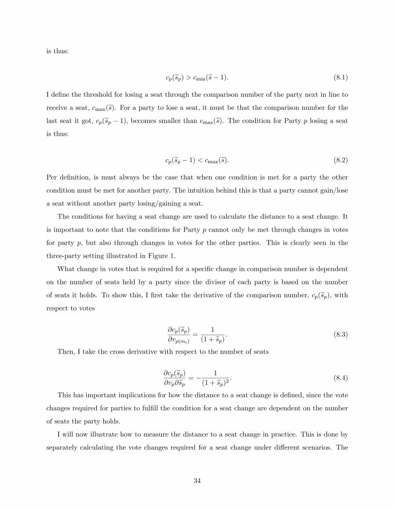
is thus:

cp(esp) > cmin(es� 1): (8.1)

I de�ne the threshold for losing a seat through the comparison number of the party next in line to

receive a seat, cmax(es). For a party to lose a seat, it must be that the comparison number for thelast seat it got, cp(esp � 1); becomes smaller than cmax(es). The condition for Party p losing a seatis thus:

cp(esp � 1) < cmax(es): (8.2)

Per de�nition, is must always be the case that when one condition is met for a party the other

condition must be met for another party. The intuition behind this is that a party cannot gain/lose

a seat without another party losing/gaining a seat.

The conditions for having a seat change are used to calculate the distance to a seat change. It

is important to note that the conditions for Party p cannot only be met through changes in votes

for party p, but also through changes in votes for the other parties. This is clearly seen in the

three-party setting illustrated in Figure 1.

What change in votes that is required for a speci�c change in comparison number is dependent

on the number of seats held by a party since the divisor of each party is based on the number

of seats it holds. To show this, I �rst take the derivative of the comparison number, cp(esp), withrespect to votes

@cp(esp)@vp(mi)

=1

(1 + esp) : (8.3)

Then, I take the cross derivative with respect to the number of seats

@cp(esp)@vp@esp = � 1

(1 + esp)2 : (8.4)

This has important implications for how the distance to a seat change is de�ned, since the vote

changes required for parties to ful�ll the condition for a seat change are dependent on the number

of seats the party holds.

I will now illustrate how to measure the distance to a seat change in practice. This is done by

separately calculating the vote changes required for a seat change under di¤erent scenarios. The

34

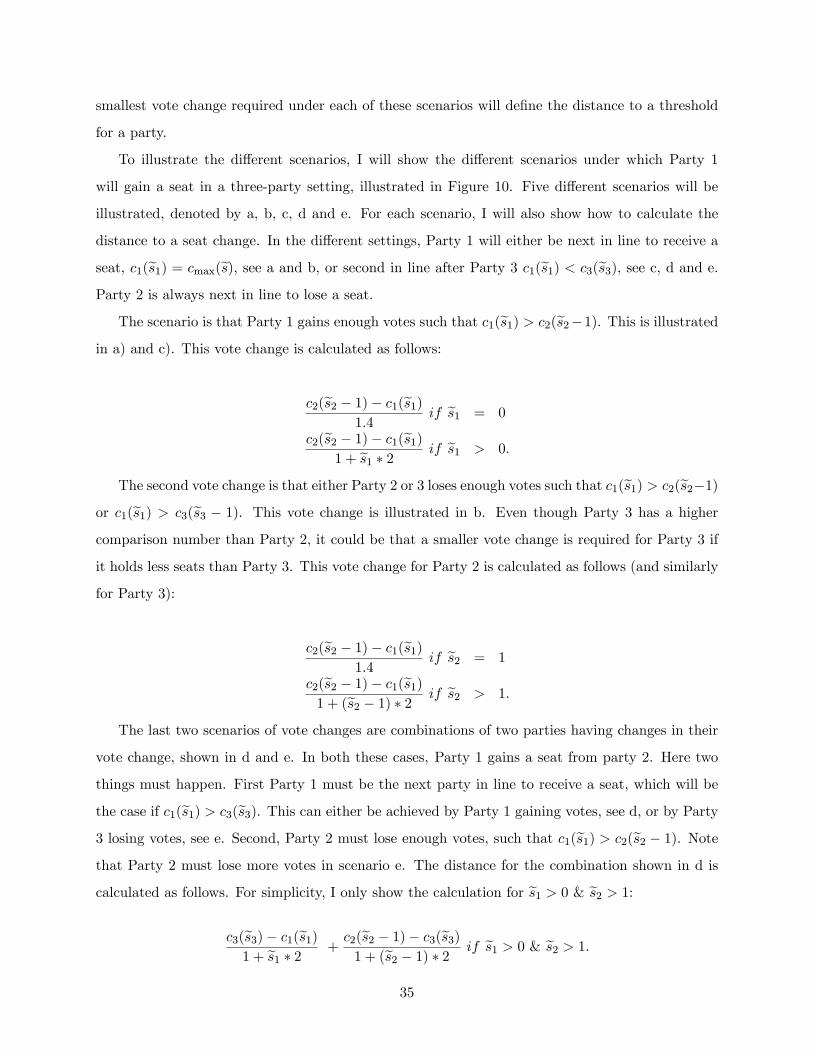
smallest vote change required under each of these scenarios will de�ne the distance to a threshold

for a party.

To illustrate the di¤erent scenarios, I will show the di¤erent scenarios under which Party 1

will gain a seat in a three-party setting, illustrated in Figure 10. Five di¤erent scenarios will be

illustrated, denoted by a, b, c, d and e. For each scenario, I will also show how to calculate the

distance to a seat change. In the di¤erent settings, Party 1 will either be next in line to receive a

seat, c1(es1) = cmax(es), see a and b, or second in line after Party 3 c1(es1) < c3(es3), see c, d and e.Party 2 is always next in line to lose a seat.

The scenario is that Party 1 gains enough votes such that c1(es1) > c2(es2�1). This is illustratedin a) and c). This vote change is calculated as follows:

c2(es2 � 1)� c1(es1)1:4

if es1 = 0

c2(es2 � 1)� c1(es1)1 + es1 � 2 if es1 > 0:

The second vote change is that either Party 2 or 3 loses enough votes such that c1(es1) > c2(es2�1)or c1(es1) > c3(es3 � 1). This vote change is illustrated in b. Even though Party 3 has a highercomparison number than Party 2, it could be that a smaller vote change is required for Party 3 if

it holds less seats than Party 3. This vote change for Party 2 is calculated as follows (and similarly

for Party 3):

c2(es2 � 1)� c1(es1)1:4

if es2 = 1

c2(es2 � 1)� c1(es1)1 + (es2 � 1) � 2 if es2 > 1:

The last two scenarios of vote changes are combinations of two parties having changes in their

vote change, shown in d and e. In both these cases, Party 1 gains a seat from party 2. Here two

things must happen. First Party 1 must be the next party in line to receive a seat, which will be

the case if c1(es1) > c3(es3). This can either be achieved by Party 1 gaining votes, see d, or by Party3 losing votes, see e. Second, Party 2 must lose enough votes, such that c1(es1) > c2(es2 � 1). Notethat Party 2 must lose more votes in scenario e. The distance for the combination shown in d is

calculated as follows. For simplicity, I only show the calculation for es1 > 0 & es2 > 1:c3(es3)� c1(es1)1 + es1 � 2 +

c2(es2 � 1)� c3(es3)1 + (es2 � 1) � 2 if es1 > 0 & es2 > 1:

35

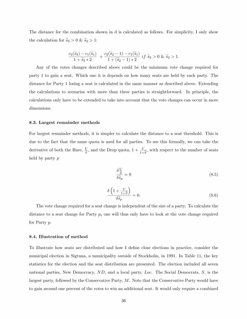
The distance for the combination shown in d is calculated as follows. For simplicity, I only show

the calculation for es3 > 0 & es2 > 1:c3(es3)� c1(es1)1 + es3 � 2 +

c2(es2 � 1)� c1(es1)1 + (es2 � 1) � 2 if es3 > 0 & es2 > 1:

Any of the votes changes described above could be the minimum vote change required for

party 1 to gain a seat. Which one it is depends on how many seats are held by each party. The

distance for Party 1 losing a seat is calculated in the same manner as described above. Extending

the calculations to scenarios with more than three parties is straightforward. In principle, the

calculations only have to be extended to take into account that the vote changes can occur in more

dimensions.

8.3. Largest remainder methods

For largest remainder methods, it is simpler to calculate the distance to a seat threshold. This is

due to the fact that the same quota is used for all parties. To see this formally, we can take the

derivative of both the Hare, VeS , and the Drop quota, 1 + V

1+eS , with respect to the number of seatsheld by party p

� VeS�esp = 0 (8.5)

��1 + V

1+eS�

�esp = 0: (8.6)

The vote change required for a seat change is independent of the size of a party. To calculate the

distance to a seat change for Party p, one will thus only have to look at the vote change required

for Party p.

8.4. Illustration of method

To illustrate how seats are distributed and how I de�ne close elections in practice, consider the

municipal election in Sigtuna, a municipality outside of Stockholm, in 1991. In Table 11, the key

statistics for the election and the seat distribution are presented. The election included all seven

national parties, New Democracy, ND, and a local party, Loc. The Social Democrats, S, is the

largest party, followed by the Conservative Party,M . Note that the Conservative Party would have

to gain around one percent of the votes to win an additional seat. It would only require a combined

36

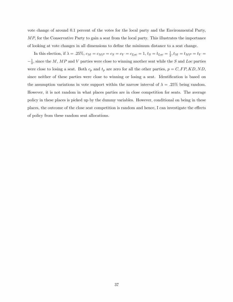
vote change of around 0.1 percent of the votes for the local party and the Environmental Party,

MP; for the Conservative Party to gain a seat from the local party. This illustrates the importance

of looking at vote changes in all dimensions to de�ne the minimum distance to a seat change.

In this election, if � = :25%, cM = cMP = cS = cV = cLoc = 1; tS = tLoc =12 ; tM = tMP = tV =

�12 ; since theM ,MP and V parties were close to winning another seat while the S and Loc parties

were close to losing a seat. Both cp and tp are zero for all the other parties, p = C;FP;KD;ND,

since neither of these parties were close to winning or losing a seat. Identi�cation is based on

the assumption variations in vote support within the narrow interval of � = :25% being random.

However, it is not random in what places parties are in close competition for seats. The average

policy in these places is picked up by the dummy variables. However, conditional on being in these

places, the outcome of the close seat competition is random and hence, I can investigate the e¤ects

of policy from these random seat allocations.

37

Figure 1. Distribution of three seats between three parties as a function of their respective vote shares. The number of seats of each party is written within each contiguous “seat outcome” region in the order Party 1, Party 2 and Party 3. Regions defined as close to a threshold for Party 1 are marked in grey. The vertical lines indicate that Party 1 is close to gaining a seat, while the horizontal line indicates its being close to losing a seat. The seats are allocated using the Sainte-Laguë method.

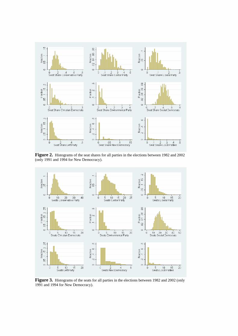
Figure 2. Histograms of the seat shares for all parties in the elections between 1982 and 2002 (only 1991 and 1994 for New Democracy).

Figure 3. Histograms of the seats for all parties in the elections between 1982 and 2002 (only 1991 and 1994 for New Democracy).

23

45

Aver

age

Seat

Sha

re (p

erce

ntag

e po

ints

) Sm

all P

artie

s

-1 -.5 0 .5 1Distance to Seat Change (percentage points) Small Parties

2224

2628

30Av

erag

e Se

at S

hare

(per

cent

age

poin

ts) L

arge

Par

ties

-1 -.5 0 .5 1Distance to Seat Change (percentage points) Large Parties

Figure 5. The voter perceived policy positions on immigration policy, environmental policy and tax policy on a scale between 0 and 10. The sizes of the markers are weighted according to the perceived importance of the policy area to each party.

Figure 4. The average seat share by the distance to a seat change, measured in percentage points of the vote share, for parties with a vote share (a) under the median size (b) and over the median size. The width of the intervals is 0.1 percentage points.

ba

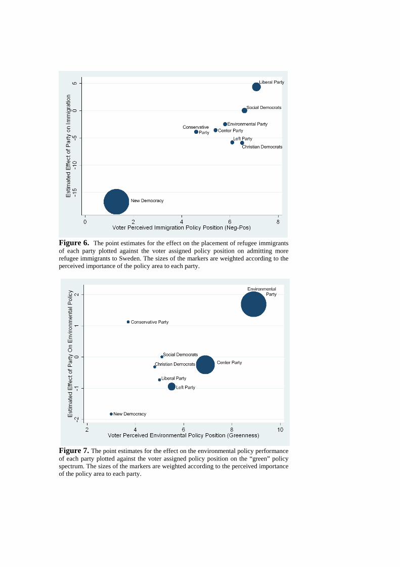
Figure 6. The point estimates for the effect on the placement of refugee immigrants of each party plotted against the voter assigned policy position on admitting more refugee immigrants to Sweden. The sizes of the markers are weighted according to the perceived importance of the policy area to each party.

Figure 7. The point estimates for the effect on the environmental policy performance of each party plotted against the voter assigned policy position on the “green” policy spectrum. The sizes of the markers are weighted according to the perceived importance of the policy area to each party.

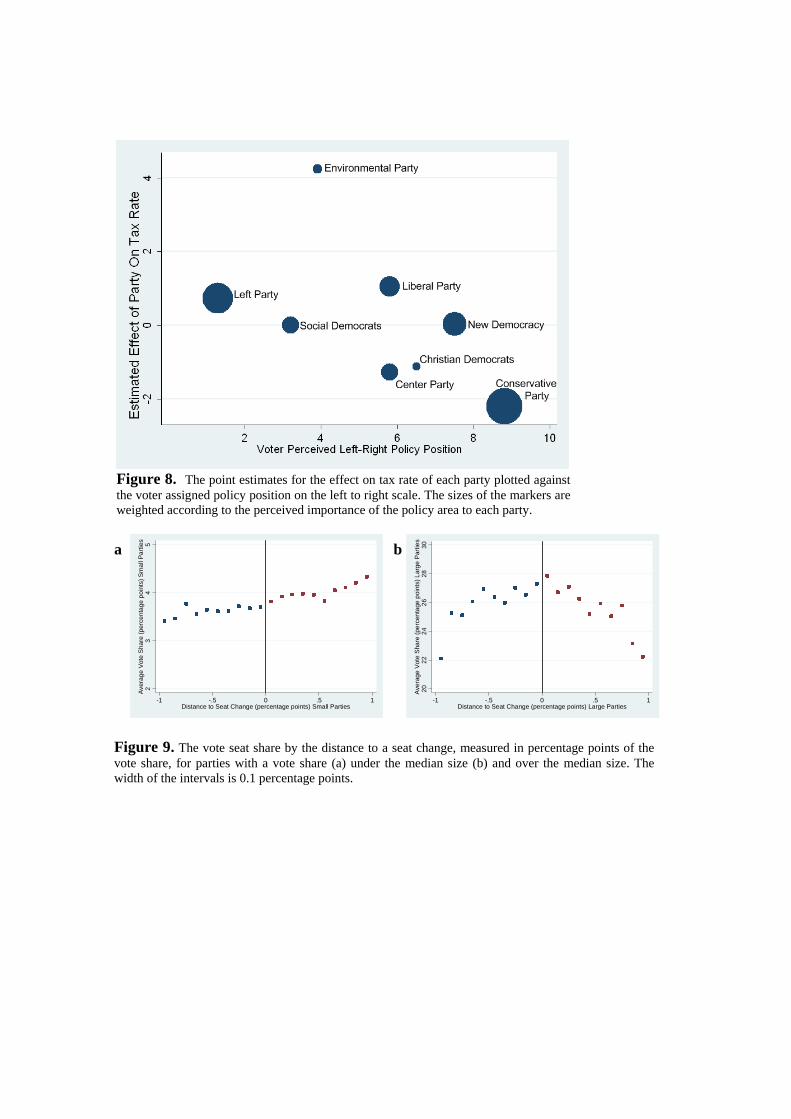
Figure 8. The point estimates for the effect on tax rate of each party plotted against the voter assigned policy position on the left to right scale. The sizes of the markers are weighted according to the perceived importance of the policy area to each party.

23

45

Aver

age

Vote

Sha

re (p

erce

ntag

e po

ints

) Sm

all P

artie

s

-1 -.5 0 .5 1Distance to Seat Change (percentage points) Small Parties

2022

2426

2830

Ave

rage

Vot

e S

hare

(per

cent

age

poin

ts) L

arge

Par

ties

-1 -.5 0 .5 1Distance to Seat Change (percentage points) Large Parties

Figure 9. The vote seat share by the distance to a seat change, measured in percentage points of the vote share, for parties with a vote share (a) under the median size (b) and over the median size. The width of the intervals is 0.1 percentage points.

ba

Figure 10. Illustration of different scenarios of vote changes leading to Party 1 gaining a seat. a) Party 1 increases its votes, such that C1(s1) > C2(s2-1) b) Either Party 2 or 3 loses votes, such that C2(s2-1) < C1(s1) or C3(s3-1) < C1(s1). c) Party 1 increases its votes such that C1(s1) > C2(s2-1). d) Party 1 increases its votes and Party 2 loses votes such that C1(s1) > C3(s3) and C2(s2-1) < C1(s1). e) Party 2 and 3 lose votes such that C3(s3) < C1(s1) and C2(s2-1) < C1(s1).

C3(s3)

C1(s1) C2(s2)

C2(s2-1)

C1(s1-1) C3(s3-1)

e)

C3(s3)

C1(s1) C2(s2)

C2(s2-1)

C1(s1-1) C3(s3-1)

d)

C3(s3)

C1(s1) C2(s2)

C2(s2-1)

C1(s1-1) C3(s3-1)

c)

C1(s1)

C3(s3) C2(s2)

C2(s2-1)

C3(s3-1) C1(s1-1)

b)

C1(s1)

C3(s3) C2(s2)

C2(s2-1)

C3(s3-1) C1(s1-1)

a)

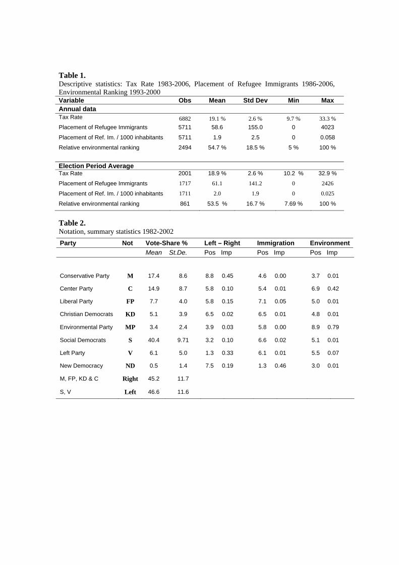
Table 1. Descriptive statistics: Tax Rate 1983-2006, Placement of Refugee Immigrants 1986-2006, Environmental Ranking 1993-2000 Variable Obs Mean Std Dev Min Max Annual data Tax Rate 6882 19.1 % 2.6 % 9.7 % 33.3 % Placement of Refugee Immigrants 5711 58.6 155.0 0 4023

Placement of Ref. Im. / 1000 inhabitants 5711 1.9 2.5 0 0.058

Relative environmental ranking 2494 54.7 % 18.5 % 5 % 100 %

Election Period Average Tax Rate 2001 18.9 % 2.6 % 10.2 % 32.9 %

Placement of Refugee Immigrants 1717 61.1 141.2 0 2426

Placement of Ref. Im. / 1000 inhabitants 1711 2.0 1.9 0 0.025

Relative environmental ranking 861 53.5 % 16.7 % 7.69 % 100 %

Table 2. Notation, summary statistics 1982-2002 Party Not Vote-Share % Left – Right Immigration Environment Mean St.De. Pos Imp Pos Imp Pos Imp

Conservative Party M 17.4 8.6 8.8 0.45 4.6 0.00 3.7 0.01

Center Party C 14.9 8.7 5.8 0.10 5.4 0.01 6.9 0.42

Liberal Party FP 7.7 4.0 5.8 0.15 7.1 0.05 5.0 0.01

Christian Democrats KD 5.1 3.9 6.5 0.02 6.5 0.01 4.8 0.01

Environmental Party MP 3.4 2.4 3.9 0.03 5.8 0.00 8.9 0.79

Social Democrats S 40.4 9.71 3.2 0.10 6.6 0.02 5.1 0.01

Left Party V 6.1 5.0 1.3 0.33 6.1 0.01 5.5 0.07

New Democracy ND 0.5 1.4 7.5 0.19 1.3 0.46 3.0 0.01

M, FP, KD & C Right 45.2 11.7

S, V Left 46.6 11.6

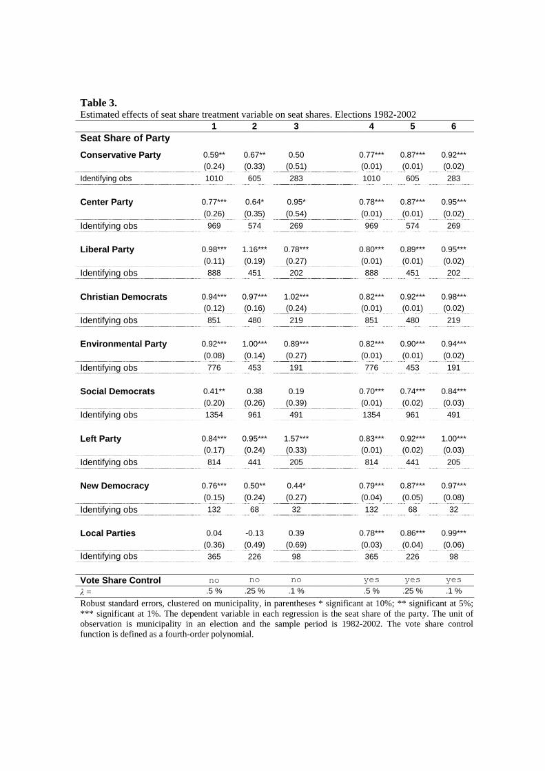
Table 3. Estimated effects of seat share treatment variable on seat shares. Elections 1982-2002

1 2 3 4 5 6 Seat Share of Party

Conservative Party 0.59** 0.67** 0.50 0.77*** 0.87*** 0.92*** (0.24) (0.33) (0.51) (0.01) (0.01) (0.02) Identifying obs 1010 605 283 1010 605 283 Center Party 0.77*** 0.64* 0.95* 0.78*** 0.87*** 0.95*** (0.26) (0.35) (0.54) (0.01) (0.01) (0.02) Identifying obs 969 574 269 969 574 269 Liberal Party 0.98*** 1.16*** 0.78*** 0.80*** 0.89*** 0.95*** (0.11) (0.19) (0.27) (0.01) (0.01) (0.02) Identifying obs 888 451 202 888 451 202 Christian Democrats 0.94*** 0.97*** 1.02*** 0.82*** 0.92*** 0.98*** (0.12) (0.16) (0.24) (0.01) (0.01) (0.02) Identifying obs 851 480 219 851 480 219 Environmental Party 0.92*** 1.00*** 0.89*** 0.82*** 0.90*** 0.94*** (0.08) (0.14) (0.27) (0.01) (0.01) (0.02) Identifying obs 776 453 191 776 453 191 Social Democrats 0.41** 0.38 0.19 0.70*** 0.74*** 0.84*** (0.20) (0.26) (0.39) (0.01) (0.02) (0.03) Identifying obs 1354 961 491 1354 961 491 Left Party 0.84*** 0.95*** 1.57*** 0.83*** 0.92*** 1.00*** (0.17) (0.24) (0.33) (0.01) (0.02) (0.03) Identifying obs 814 441 205 814 441 205 New Democracy 0.76*** 0.50** 0.44* 0.79*** 0.87*** 0.97*** (0.15) (0.24) (0.27) (0.04) (0.05) (0.08) Identifying obs 132 68 32 132 68 32 Local Parties 0.04 -0.13 0.39 0.78*** 0.86*** 0.99*** (0.36) (0.49) (0.69) (0.03) (0.04) (0.06) Identifying obs 365 226 98 365 226 98 Vote Share Control no no no yes yes yes

λ = .5 % .25 % .1 % .5 % .25 % .1 % Robust standard errors, clustered on municipality, in parentheses * significant at 10%; ** significant at 5%; *** significant at 1%. The dependent variable in each regression is the seat share of the party. The unit of observation is municipality in an election and the sample period is 1982-2002. The vote share control function is defined as a fourth-order polynomial.

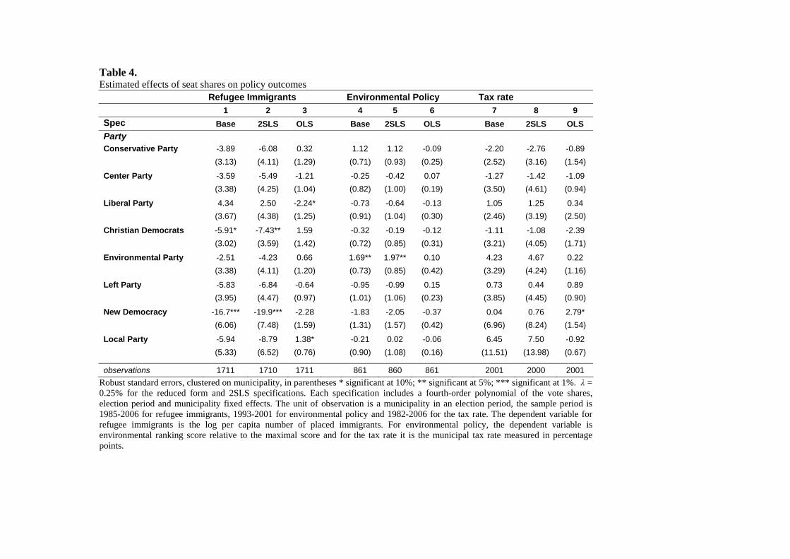
Table 4. Estimated effects of seat shares on policy outcomes

Refugee Immigrants Environmental Policy Tax rate 1 2 3 4 5 6 7 8 9

Spec Base 2SLS OLS Base 2SLS OLS Base 2SLS OLS Party Conservative Party -3.89 -6.08 0.32 1.12 1.12 -0.09 -2.20 -2.76 -0.89 (3.13) (4.11) (1.29) (0.71) (0.93) (0.25) (2.52) (3.16) (1.54)

Center Party -3.59 -5.49 -1.21 -0.25 -0.42 0.07 -1.27 -1.42 -1.09 (3.38) (4.25) (1.04) (0.82) (1.00) (0.19) (3.50) (4.61) (0.94)

Liberal Party 4.34 2.50 -2.24* -0.73 -0.64 -0.13 1.05 1.25 0.34 (3.67) (4.38) (1.25) (0.91) (1.04) (0.30) (2.46) (3.19) (2.50)

Christian Democrats -5.91* -7.43** 1.59 -0.32 -0.19 -0.12 -1.11 -1.08 -2.39 (3.02) (3.59) (1.42) (0.72) (0.85) (0.31) (3.21) (4.05) (1.71)

Environmental Party -2.51 -4.23 0.66 1.69** 1.97** 0.10 4.23 4.67 0.22 (3.38) (4.11) (1.20) (0.73) (0.85) (0.42) (3.29) (4.24) (1.16)

Left Party -5.83 -6.84 -0.64 -0.95 -0.99 0.15 0.73 0.44 0.89 (3.95) (4.47) (0.97) (1.01) (1.06) (0.23) (3.85) (4.45) (0.90)

New Democracy -16.7*** -19.9*** -2.28 -1.83 -2.05 -0.37 0.04 0.76 2.79* (6.06) (7.48) (1.59) (1.31) (1.57) (0.42) (6.96) (8.24) (1.54)

Local Party -5.94 -8.79 1.38* -0.21 0.02 -0.06 6.45 7.50 -0.92

(5.33) (6.52) (0.76) (0.90) (1.08) (0.16) (11.51) (13.98) (0.67)

observations 1711 1710 1711 861 860 861 2001 2000 2001 Robust standard errors, clustered on municipality, in parentheses * significant at 10%; ** significant at 5%; *** significant at 1%. λ = 0.25% for the reduced form and 2SLS specifications. Each specification includes a fourth-order polynomial of the vote shares, election period and municipality fixed effects. The unit of observation is a municipality in an election period, the sample period is 1985-2006 for refugee immigrants, 1993-2001 for environmental policy and 1982-2006 for the tax rate. The dependent variable for refugee immigrants is the log per capita number of placed immigrants. For environmental policy, the dependent variable is environmental ranking score relative to the maximal score and for the tax rate it is the municipal tax rate measured in percentage points.

Table 5. Difference in representation effects between pairs of parties. Refugee Immigrants Environmental Policy Tax rate 1 2 3 4 5 6 Gain

Party Liberal Party

New Demo

Environ Party

Center Party

Conser Party

Left Party

Lose Conservative Party 8.2 -12.8 0.6 -1.4 2.9 (0.06) (0.04) (0.58) (0.16) (0.53)

Center Party 7.9 -13.1 2 -0.9 2 (0.08) (0.05) (0.05) (0.84) (0.58)

Liberal Party -21 2.4 0.4 -3.3 -0.4 (0.00) (0.05) (0.68) (0.36) (0.94)

Christian Democrats 10.2 -10.8 2 0 -1.1 1.8 (0.03) (0.09) (0.04) (0.95) (0.78) (0.67)

Environmental Party 6.8 -14.2 -2 -6.4 -3.5 (0.16) (0.05) (0.05) (0.10) (0.33)

Social Democrats 4.3 -16.7 1.7 -0.3 -2.2 (0.7 (0.24) (0.01) (0.02) (0.76) (0.38) (0.85)

Left Party 10.1 -10.9 2.6 0.6 -2.9 (0.03) (0.10) (0.04) (0.58) (0.53)

New Democracy 21 3.5 1.5 -2.2 0.7 (0.00) (0.03) (0.29) (0.76) (0.93)

Local Party 10.2 -10.8 1.9 -0.1 -8.7 -5.8

(0.12) (0.19) (0.08) (0.97) (0.47) (0.59)

The results from the baseline specification, shown in table 4, are used to construct the table. The effect of each party gaining a seat relative to each other party is shown in the columns, while the effect of losing a seat is shown in the rows. The differences that are significant at the 10% level are highlighted in bold. The P-values from F-tests for differences in effects between pair of parties are shown in parentheses.

Table 6. Estimated effects of seat shares on the placement of refugee immigrants 1986-2006, alternative specifications

λ = 0.5% 0.25 % 0.1% 1 2 3 4 5 6 7 8 9

Conservative Party -2.56 -1.30 -6.30 -4.12 -5.41 -3.89 -4.01 -3.48 -0.64 (2.61) (2.40) (4.92) (4.41) (3.43) (3.13) (3.19) (5.16) (4.62)

Center Party -0.31 -0.92 -4.43 -3.97 -3.33 -3.59 -3.38 0.08 -3.25 (2.81) (2.51) (5.35) (4.88) (4.03) (3.38) (3.36) (6.30) (5.61)

Liberal Party 0.60 0.59 5.57 6.19 3.20 4.34 4.18 10.16* 8.99 (2.63) (2.53) (5.36) (4.86) (3.92) (3.67) (3.61) (5.96) (5.87)

Christian Democrats -2.27 -1.14 -9.3** -8.71* -5.92* -5.91* -6.24** -8.28 -9.55** (2.78) (2.49) (4.53) (4.43) (3.54) (3.02) (3.04) (5.79) (4.72)

Environmental Party 0.06 -2.45 -1.90 1.57 -0.03 -2.51 -2.44 -1.96 2.53 (2.59) (2.37) (5.43) (4.60) (3.89) (3.38) (3.41) (6.78) (5.39)

Left Party -2.98 -1.70 -9.62* -8.68* -11.8*** -5.83 -5.83 -8.93 -2.53 (2.85) (2.69) (5.73) (4.89) (4.00) (3.95) (3.93) (5.81) (5.67)

New Democracy -8.61 -9.64** -13.1 -14.1 -18.8** -16.7*** -16.9*** -9.72 -13.4** (6.25) (4.46) (10.2) (11.57) (8.41) (6.06) (6.01) (6.18) (6.41)

Local Party -9.23** -7.09* -16.7** -14.9** -7.00 -5.94 -6.23 0.29 2.11 (4.45) (3.71) (8.29) (7.37) (6.47) (5.33) (5.38) (8.57) (7.79)

Vote Share Control yes yes no yes yes yes yes yes yes Election Period F.E yes yes no no yes yes yes yes yes Municipality F.E no yes no no no yes yes no yes Control Varaibles no no no no no no yes no no observations 1711 1711 1711 1711 1711 1711 1711 1711 1711

Robust standard errors, clustered on municipality, in parentheses * significant at 10%; ** significant at 5%; *** significant at 1%. The dependent variable is the log of the number of placed immigrants per capita. The unit of observation is a municipality in an election period and the sample period is 1985-2006.

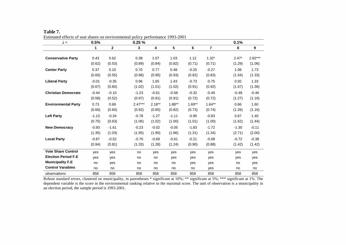
Table 7. Estimated effects of seat shares on environmental policy performance 1993-2001

λ = 0.5% 0.25 % 0.1% 1 2 3 4 5 6 7 8 9

Conservative Party 0.43 0.62 0.38 1.07 1.03 1.12 1.32* 2.47* 2.82*** (0.62) (0.53) (0.89) (0.84) (0.82) (0.71) (0.71) (1.29) (1.06)

Center Party 0.37 0.10 0.70 0.77 0.48 -0.25 -0.27 1.06 1.73 (0.65) (0.55) (0.98) (0.95) (0.93) (0.82) (0.83) (1.54) (1.33)

Liberal Party -0.01 -0.35 0.96 1.65 1.43 -0.73 -0.75 0.92 1.33 (0.67) (0.60) (1.02) (1.01) (1.02) (0.91) (0.92) (1.67) (1.36)

Christian Democrats -0.44 -0.10 -1.23 -0.61 -0.58 -0.32 -0.49 -0.48 -0.46 (0.58) (0.52) (0.97) (0.91) (0.91) (0.72) (0.72) (1.27) (1.16)

Environmental Party 0.73 0.69 2.47*** 2.18** 1.88** 1.69** 1.64** 0.66 1.60 (0.66) (0.60) (0.92) (0.85) (0.82) (0.73) (0.74) (1.26) (1.16)

Left Party -1.13 -0.34 -0.78 -1.27 -1.11 -0.95 -0.83 0.67 1.40 (0.75) (0.63) (1.06) (1.02) (1.00) (1.01) (1.00) (1.62) (1.44)

New Democracy -0.93 -1.61 -0.23 -0.02 -0.05 -1.83 -1.72 -1.30 -0.11 (1.35) (1.03) (1.95) (1.90) (1.86) (1.31) (1.34) (2.71) (2.00)

Local Party -0.87 -0.52 -0.76 -0.69 -0.61 -0.21 -0.08 -0.72 -0.38 (0.94) (0.81) (1.33) (1.28) (1.24) (0.90) (0.88) (1.42) (1.42)

Vote Share Control yes yes no yes yes yes yes yes yes Election Period F.E yes yes no no yes yes yes yes yes Municipality F.E no yes no no no yes yes no yes Control Varaibles no no no no no no yes no no observations 858 858 858 858 858 858 858 858 858

Robust standard errors, clustered on municipality, in parentheses * significant at 10%; ** significant at 5%; *** significant at 1%. The dependent variable is the score in the environmental ranking relative to the maximal score. The unit of observation is a municipality in an election period, the sample period is 1993-2001.

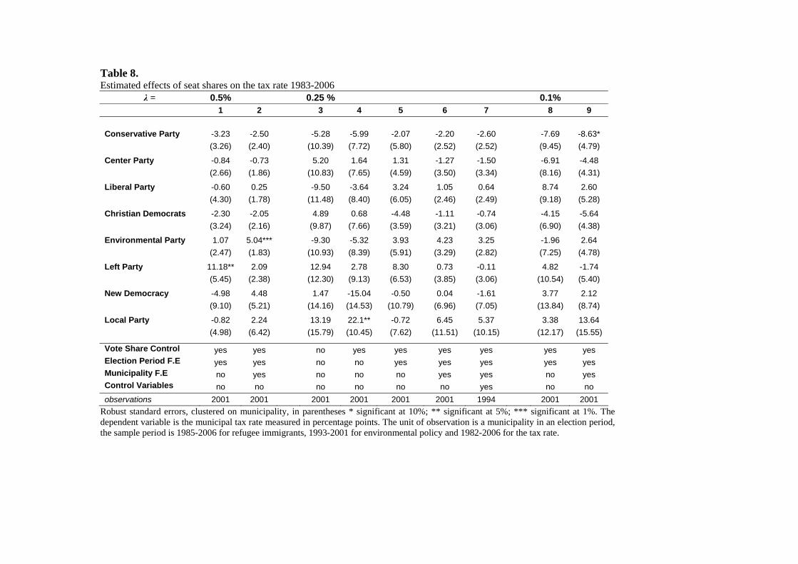
Table 8. Estimated effects of seat shares on the tax rate 1983-2006

λ = 0.5% 0.25 % 0.1% 1 2 3 4 5 6 7 8 9

Conservative Party -3.23 -2.50 -5.28 -5.99 -2.07 -2.20 -2.60 -7.69 -8.63* (3.26) (2.40) (10.39) (7.72) (5.80) (2.52) (2.52) (9.45) (4.79)

Center Party -0.84 -0.73 5.20 1.64 1.31 -1.27 -1.50 -6.91 -4.48 (2.66) (1.86) (10.83) (7.65) (4.59) (3.50) (3.34) (8.16) (4.31)

Liberal Party -0.60 0.25 -9.50 -3.64 3.24 1.05 0.64 8.74 2.60 (4.30) (1.78) (11.48) (8.40) (6.05) (2.46) (2.49) (9.18) (5.28)

Christian Democrats -2.30 -2.05 4.89 0.68 -4.48 -1.11 -0.74 -4.15 -5.64 (3.24) (2.16) (9.87) (7.66) (3.59) (3.21) (3.06) (6.90) (4.38)

Environmental Party 1.07 5.04*** -9.30 -5.32 3.93 4.23 3.25 -1.96 2.64 (2.47) (1.83) (10.93) (8.39) (5.91) (3.29) (2.82) (7.25) (4.78)

Left Party 11.18** 2.09 12.94 2.78 8.30 0.73 -0.11 4.82 -1.74 (5.45) (2.38) (12.30) (9.13) (6.53) (3.85) (3.06) (10.54) (5.40)

New Democracy -4.98 4.48 1.47 -15.04 -0.50 0.04 -1.61 3.77 2.12 (9.10) (5.21) (14.16) (14.53) (10.79) (6.96) (7.05) (13.84) (8.74)

Local Party -0.82 2.24 13.19 22.1** -0.72 6.45 5.37 3.38 13.64 (4.98) (6.42) (15.79) (10.45) (7.62) (11.51) (10.15) (12.17) (15.55)

Vote Share Control yes yes no yes yes yes yes yes yes Election Period F.E yes yes no no yes yes yes yes yes Municipality F.E no yes no no no yes yes no yes Control Variables no no no no no no yes no no observations 2001 2001 2001 2001 2001 2001 1994 2001 2001

Robust standard errors, clustered on municipality, in parentheses * significant at 10%; ** significant at 5%; *** significant at 1%. The dependent variable is the municipal tax rate measured in percentage points. The unit of observation is a municipality in an election period, the sample period is 1985-2006 for refugee immigrants, 1993-2001 for environmental policy and 1982-2006 for the tax rate.

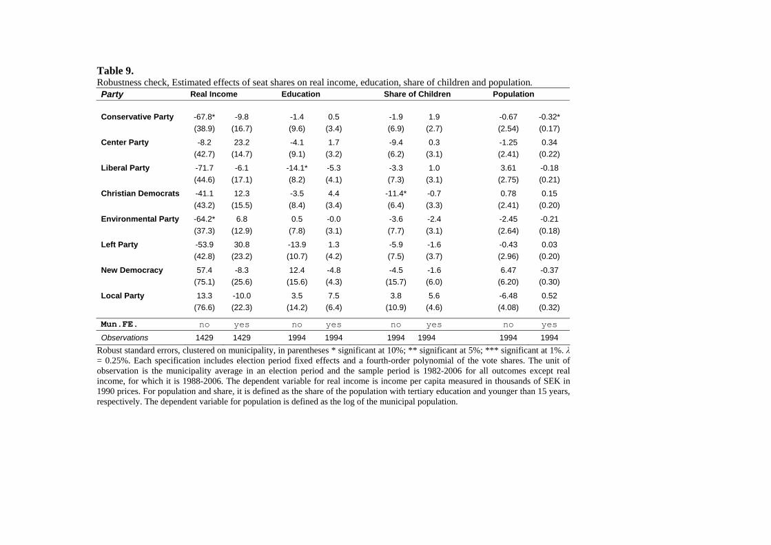
Table 9. Robustness check, Estimated effects of seat shares on real income, education, share of children and population. Party Real Income Education Share of Children Population Conservative Party -67.8* -9.8 -1.4 0.5 -1.9 1.9 -0.67 -0.32* (38.9) (16.7) (9.6) (3.4) (6.9) (2.7) (2.54) (0.17)

Center Party -8.2 23.2 -4.1 1.7 -9.4 0.3 -1.25 0.34 (42.7) (14.7) (9.1) (3.2) (6.2) (3.1) (2.41) (0.22)

Liberal Party -71.7 -6.1 -14.1* -5.3 -3.3 1.0 3.61 -0.18 (44.6) (17.1) (8.2) (4.1) (7.3) (3.1) (2.75) (0.21)

Christian Democrats -41.1 12.3 -3.5 4.4 -11.4* -0.7 0.78 0.15 (43.2) (15.5) (8.4) (3.4) (6.4) (3.3) (2.41) (0.20)

Environmental Party -64.2* 6.8 0.5 -0.0 -3.6 -2.4 -2.45 -0.21 (37.3) (12.9) (7.8) (3.1) (7.7) (3.1) (2.64) (0.18)

Left Party -53.9 30.8 -13.9 1.3 -5.9 -1.6 -0.43 0.03 (42.8) (23.2) (10.7) (4.2) (7.5) (3.7) (2.96) (0.20)

New Democracy 57.4 -8.3 12.4 -4.8 -4.5 -1.6 6.47 -0.37 (75.1) (25.6) (15.6) (4.3) (15.7) (6.0) (6.20) (0.30)

Local Party 13.3 -10.0 3.5 7.5 3.8 5.6 -6.48 0.52 (76.6) (22.3) (14.2) (6.4) (10.9) (4.6) (4.08) (0.32)

Mun.FE. no yes no yes no yes no yes

Observations 1429 1429 1994 1994 1994 1994 1994 1994 Robust standard errors, clustered on municipality, in parentheses * significant at 10%; ** significant at 5%; *** significant at 1%. λ = 0.25%. Each specification includes election period fixed effects and a fourth-order polynomial of the vote shares. The unit of observation is the municipality average in an election period and the sample period is 1982-2006 for all outcomes except real income, for which it is 1988-2006. The dependent variable for real income is income per capita measured in thousands of SEK in 1990 prices. For population and share, it is defined as the share of the population with tertiary education and younger than 15 years, respectively. The dependent variable for population is defined as the log of the municipal population.

Table 10. Heterogeneous representation effects with respect to winning the first seat. 1 2 3

Treatment Variable

Share of Observation

Refugee Immigrants Environmental

Policy Tax rate

Conservative Party Seat Share 99% -2.84 1.23 -2.53 (3.22) (0.76) (2.65) First Seat 1% -120*** 0.00 -13.84 (28.1) (0.00) (32.38)

Center Party Seat Share 97% -2.49 -0.28 -1.25 (3.38) (0.86) (3.72) First Seat 3% -31.04 7.48 -18.96 (21.27) (5.52) (13.30)

Liberal Party Seat Share 94% 3.81 -0.92 -1.34 (3.79) (0.95) (2.76) First Seat 6% -35.2 0.03 31.84* (33.2) (7.60) (17.00)

Christian Democrats Seat Share 72% -2.13 -0.91 0.68 (3.71) (0.86) (4.02) First Seat 28% -9.63 2.92* -5.11 (8.55) (1.76) (6.39)

Environmental Party Seat Share 70% -3.58 2.44** 4.05

(3.93) (0.94) (3.52)

First Seat 30% -2.33 -6.11*** -1.71 (6.84) (2.04) (5.25)

Left Party Seat Share 87% -7.14* -1.57 1.72

(4.33) (1.04) (4.51)

First Seat 13% 15.99* 4.92** -5.53 (9.66) (2.27) (8.13)

New Democracy Seat Share 43% -22.00 -1.07 -5.37

(13.74) (1.98) (12.50)

First Seat 57% 12.86 -4.55 13.01 (15.99) (2.80) (16.58)

Local parties Seat Share 85% -4.56 -0.49 12.39

(6.07) (1.05) (12.26)

First Seat 15% 18.05 1.05 -36.89 (16.88) (5.33) (32.57)

Observations 1711 861 2001 Robust standard errors, clustered on municipality, in parentheses * significant at 10%; ** significant at 5%; *** significant at 1%. d = 0.25%. The treatment variable labeled seat share is the seat share treatment variable from the baseline specification. The treatment variable labeled first seat is the dummy for being close to the threshold for the first seat interacted with the seat share treatment variable. Each specification includes a fourth-order polynomial of the vote shares, dummy variables for each party being close to the threshold for the first seat, election period and municipality fixed effects. The unit of observation is a municipality in an election period, the sample period is 1985-2006 for refugee immigrants, 1993-2001 for environmental policy and 1982-2006 for the tax rate.

Table 11. Election Data from Sigtuna 1991. Party Cons. Cent. Lib. Chr. Env. Soc. Left N. D. Local Vote Share % 31.24 6.21 9.59 3.71 3.04 36.64 2.96 4.79 3.11

Seats 15.00 3.00 5.00 2.00 1.00 18.00 1.00 2.00 2.00

Seat Share % 3.61 6.12 1.20 4.08 2.04 36.73 2.04 4.08 4.08

Dis gain ind % .92 1.05 1.82 1.47 .08 1.75 .16 .40 2.07

Dis gain all % .10 .95 1.62 1.42 .08 .75 .16 .35 2.02

Dis lose ind % 1.88 1.15 .48 .68 1.62 1.21 1.54 1.75 .08

Note:. "Dis gain ind" and "Dis lose ind" is the distance to a threshold measured in the individual parties’ votes. "Dis gain all" and "Dis lose all" are the distance to a threshold measured in percentage points. The distance measure is in bold if the party is within .25% of a threshold.