sfdg - Brands Delmar - Cengage Learning€¦ · Web viewPlace the word PARAM adjacent to R4....

Notes Click to select desired

section or chapter Vol 1 refers to Circuit

Analysis, while Vol 2 refers to Circuit Analysis with Devices

Chapters 1 to 23 are common to both books

Background Notes1. Cadence Design Systems (who

owns the OrCad trademark) has created two schematic capture interface programs, Capture (as described in the text book) and Schematics (as described here).

2. Capture and Schematics have both been bundled into the PSpice student software package. When you invoke PSpice on your computer, you must select the one that you wish to use.

3. In the Robbins and Miller books, we have used Capture; on this web site, we provide duplicate coverage using Schematics.)

On-Line Companion: PSpice Using Schematics

As you now know, to analyze a problem using PSpice, you

must first create its circuit on your screen, a process referred to

as “schematic capture”. The purpose of this web site is to show

you how to use the PSPice Schematics editor for this task (see

Background Notes).

Index

Section I: A Short Overview of Schematics

Section II: Worked Out PSPice Examples Using Schematics

Chapter 4 Chapter 5 Chapter 6 Chapter 7 Chapter 8 Chapter 9 Chapter 11 Chapter 14 Chapter 15 Chapter 16 Chapter 17 Chapter 18 Chapter 19 Chapter 20 Chapter 21 Chapter 22 Chapter 23 Chapter 24 (Vol 1) Chapter 25 (Vol 2) Chapter 26 (Vol 2) Chapter 27 (Vol 2) Chapter 28 (Vol 2) Chapter 29 (Vol 2) Chapter 30 (Vol 2)

Robbins/ Miller On-Line Comapnion 1 Nov 2003 (Revised Jan 4/04)

Saving PSpice files

As noted in Appendix A of the text book, we recommend that you use a separate folder for each PSpice problem or group of problems in order to contain the clutter of intermediate files that PSpice creates.

Section I: A Short Overview of SchematicsSection I is for reference. If you are new to PSpice, you should browse through it for

general information before you try the examples of Section II. (Because it is a reference

document, you may find things that you have not yet covered. For example, if you are

reading this while studying dc, you will not understand the comments regarding ac, etc.

Just ignore these and return to them later when you get to that part of your course.). In

what follows, we assume that you have PSpice loaded on your computer with the

Schematics icon on your screen. (If you do not have the icon on your screen, click Start,

select Programs, PSpice Student then Schematics.) To analyze a circuit, use the following

general procedure:

1. Click the Schematics icon on your screen. This opens the PSpice editor,

Figure I-1.

2. Create the circuit on your screen.

3. Save your work to an appropriately named file – see box.

4. Specify the type of analysis that you wish to perform

5. Set up the analysis parameters, perform the analysis, then

view the results

There are generally several ways to do many things. The approaches

shown below will get you started.


The Schematics Screen

When you click the Schematics icon, a screen similar to that shown in Figure I-1 should

open.

Note the menu items and icons. To familiarize yourself with these, place your mouse pointer over each in

turn. As you do, a text box opens to tell you what the selected item’s function is. After you have

familiarized yourself with these, review the PSpice information in Appendix A of the text, starting at the

section entitled “Some Key Points for PSpice Users”.

Other Things to Note

Mouse Buttons: Use the left mouse button for all operations unless directed otherwise.


Keyboard entries: Frequently, you are instructed to type values into dialog boxes. In the

examples that follow, these are shown in bold face. Thus, 25V indicates a value that you

type in via the keyboard.

Get and Place a Part: To get and place a new part, click the Get New Part button and

when the Parts Browser dialog box opens, select the desired part (source, resistor,

capacitor, etc). You can do this by clicking on the item in the parts list, (or you can type

in its abbreviation, R for resistor, C for capacitor, etc.), then click Place or Place & Close

(or press the Enter key). Position the component as desired on the window, then click the

left button. If you wish to place more than one instance of the component, repeat for each

placement. When done, click the right button to end placement of that component.

Get Recent Part Bin: PSpice keeps track of the most recent parts used and lists them in

the Get Recent Part bin. You can save time by selecting items from this bin. Simply

double click the item then place as described above.


Meter Elements IPRINT, VPRINT1 and VPRINT2: These are general purpose

metering components that you can use to measure voltage and current. To determine their

readings, you must examine the output file. (Click Analysis, Examine Output, then scroll

until you find them.) Note that IPRINT and VPRINT1 have a terminal marked with a

sign that corresponds to the COM terminal on a real physical meter. You must wire them

into your circuit as you would a real meter, taking into account where you want the COM

terminal. In addition, you must configure them for the type of measurement (dc or ac)

that you wish to make. This is described in the examples that follow.


Netlists: When PSpice creates a circuit description from your schematic, it numbers

nodes and for each component, lists the nodes to which it is connected as well as the

value of the component. (For example, Node 1 is designated $N001, node 2 as $N002,

etc.) These designations do not appear on your schematic screen but instead they reside in

a file as a “netlist”. (To view, click Analysis, then Examine Netlist.) In the netlist, the “1”

end of a component is connected to the first indicated node.) The netlist can serve as a

useful troubleshooting aid; if PSpice displays an error message after simulation and you

need more information, click Analysis, Examine Output then check for error details.)

Section II: Worked Out PSpice Examples Using Schematics

For the most part, Schematics screen displays are similar to those created by Capture and

thus (except for the first few examples), we will rely on the photos in the book. For the

instructions that follow, icons and menu items referred to may be identified by reference

to the user interface screen of Figure I-1 shown earlier (Section I).

Chapter 4 Ohm’s Law

PSpice provides two methods for solving dc problems, the bias point method and the DC

Sweep method. We illustrate both. Since this is our first look at computer simulation, we

include considerable detail.


Operational Notes1. The resistor should be rotated

before it is placed so that its “1” end is at the top (see Appendix A of the textbook). To rotate it, hold down the Control key and type R, an operation we henceforth designate as Ctrl/R. If the resistor does not rotate, it may have become deselected. If this is the case, select it again as in Note 2, then rotate.

2. To select a component for any reason (e.g., to reposition it or to delete it), place your mouse pointer on the component, then left click. (It turns red to indicate that it is selected).

3. If you make a mistake and need to delete a component, or a wire, select it as in Note 2, then press the Delete key on your keyboard.

First Example (Bias Point Analysis)

Determine current for the circuit of Figure 4-27 of the book using the bias point method.

Procedure: Click the Schematics icon to call up PSpice and get the opening screen on

your computer. Now construct the circuit of Figure 4-29 of the text (also shown in Figure

I-1 of these notes) as follows:

Click the Get New Part button and in the browser Part Name window, type vdc to

select the dc source, then press the Enter key on your keyboard. (You can also click

its name on the browser scroll list.) Alternately, if the source is already in the Recent

Parts bin, you can get it from there by clicking it in the drop-down box.

Move the mouse pointer into the drawing area and position the source where you

want it. Click the left mouse button to place, then click

the right mouse button to end placement. (The battery

has a default voltage of 0V. We will change it shortly.)

To get the resistor, repeat the first step above except

type R in the Part Name window.

Rotate the resistor three times to provide for correct

node assignments – see box, Note 1. Position the

resistor where desired, click the left mouse button to

place it, then click the right mouse button to end

placement.

To get the ground symbol, repeat the first step except

type egnd. A ground symbol appears. Position it on the screen with a left click then

click right.


To wire the circuit, click the Draw Wire button. A pencil appears. Position it at the

end of the lead protruding from the top of the battery, click left to start placement,

then drag the pencil to the end of the lead at the top of the resistor. As you drag, a

dashed line follows. Click left when you reach the resistor lead. This places the

wire. (To help control routing, you can click the left button to freeze the wire in

place as you drag it, as for example when you want to turn a corner.) Similarly,

place a wire between the bottom of the source and the ground, then place a wire

from the bottom end of the resistor to the wire just placed. (You should now have

the circuit of Figure I-1.) Click right button to end placement.

If you want to reposition a component or wire to improve the layout of your circuit,

select the component as in Operational Note 2, drag it to its new location then

release the button. Repeat for any other items that need moved.

The battery default voltage is 0V. To change it, double click its voltage value.

(Make sure you double click 0V, not the battery symbol.) A Set Attribute Value

dialog box opens. Type 25V then press Enter or click OK. (The unit V can be

omitted if desired. If you include the symbol V, do not leave a space. Thus, 25 V is

unacceptable.) Repeat the process and set the resistor to 12.5ohm.

Click the Save button and save your work under an appropriate file name such as

figure 4-29 in an appropriate file folder. (See Note 11 on page 105 of the text.)

Now run the simulation. To do this, click the Simulate button. After a short

execution time, an inactive Output window may open. If so, close it.


On the menu bar, click the Enable Bias Current Display button. Computed currents

are displayed as in Figure 4-29 of the text. Now click the Enable Bias Voltage

Display button and circuit voltages will appear.

To exit from PSpice, click the in the upper right hand corner of the screen and

click yes to save changes (if asked).

Second Example (DC Sweep Analysis)

You can also solve the problem of Figure 4-27 using the DC Sweep method. First, call up

PSpice to get the opening screen, then build the circuit as in Figure 4-30 of the text.

(IPRINT is a general-purpose ammeter that you get by clicking Get New Part. Type

IPRINT and place as indicated.)

You need to configure IPRINT for dc operation. Double click its symbol and a

dialog box opens. Double click DC = and in the Value box type yes, click Save Attr,

then click OK. The box closes. The meter has now been set for dc operation.

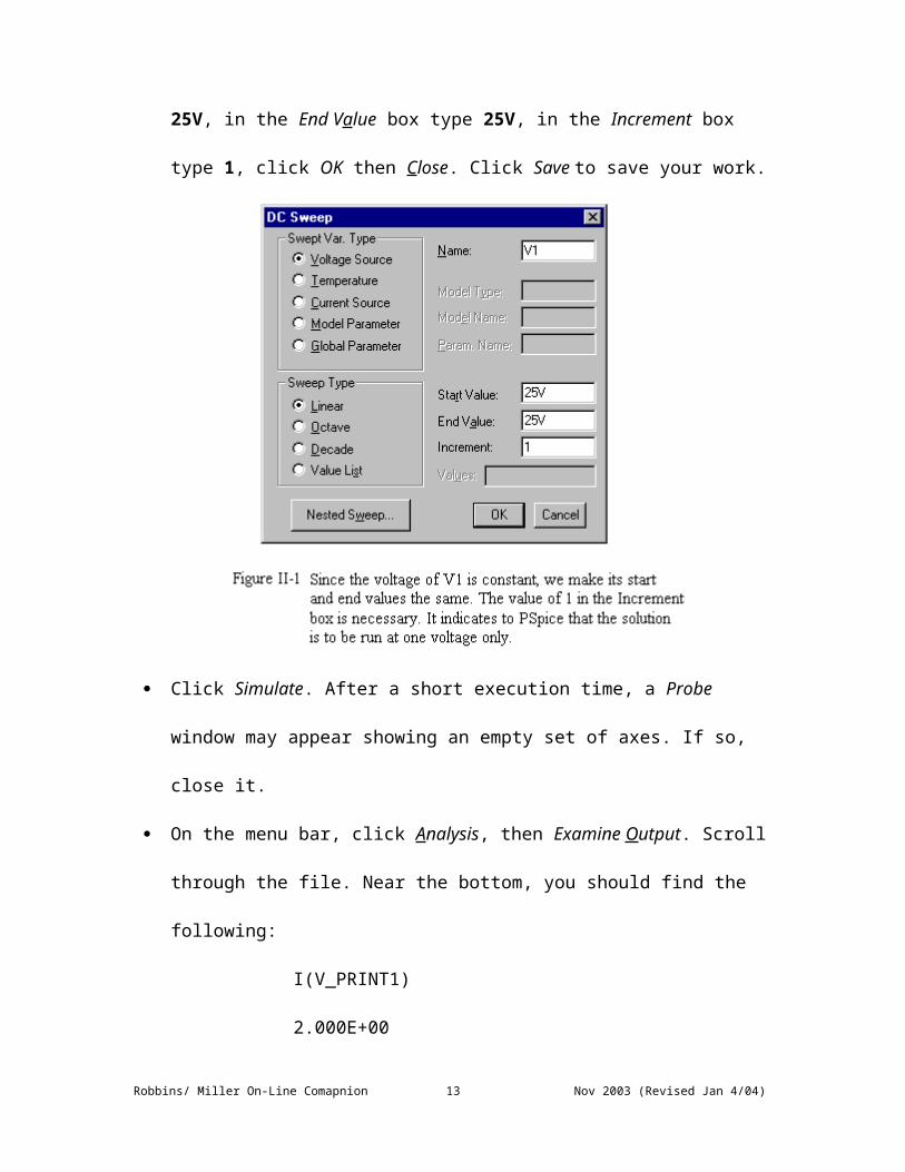
Click Setup Analysis and in the Analysis Setup dialog box that opens, click DC

Sweep. A dialog box opens, Figure II-1. In the Name box, type the name of your

source. (Check the schematic on your screen. The source is likely labeled V1. Enter

this.) In the Start Value box type 25V, in the End Value box type 25V, in the

Increment box type 1, click OK then Close. Click Save to save your work.


Click Simulate. After a short execution time, a Probe window may appear showing

an empty set of axes. If so, close it.

On the menu bar, click Analysis, then Examine Output. Scroll through the file. Near

the bottom, you should find the following:

I(V_PRINT1)

2.000E+00

This is the answer. The I(V_PRINT1) refers to the IPRINT meter and the answer

2.000E+00 is the current that it measured. Thus, for this circuit, PSpice determined I = 2

A as expected.


NoteIt is not always possible to place the cursor exactly where you want it (because of the nature of simulation programs). You may have to set it as closely as you can get then estimate the value that you are trying to measure.

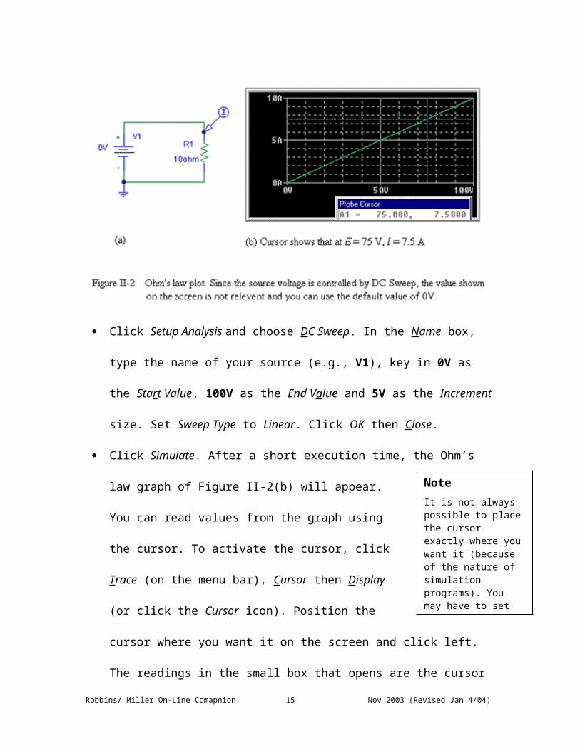
Third Example (Ohm’s Law Plot)

PSpice can graph results. By varying the voltage of the source and plotting current for

example, you can get an Ohm’s law plot.

Build the circuit of Figure II-2(a). Click the Current Marker Probe button and place

the marker at the top end of the resistor as shown. Save your work as file figure II-2

(or a file name of your own choosing).

Click Setup Analysis and choose DC Sweep. In the Name box, type the name of your

source (e.g., V1), key in 0V as the Start Value, 100V as the End Value and 5V as

the Increment size. Set Sweep Type to Linear. Click OK then Close.

Click Simulate. After a short execution time, the Ohm’s law graph of Figure II-2(b)

will appear. You can read values from the graph using the cursor.

To activate the cursor, click Trace (on the menu bar), Cursor

then Display (or click the Cursor icon). Position the cursor

where you want it on the screen and click left. The readings in


the small box that opens are the cursor coordinates. The first number represents the

x-axis reading (voltage) and the second the y-axis reading (current). Position the

cursor at various voltages, read the results and verify using your calculator.

Chapter 5 Series Circuits (Example 5-15)

Using the bias point analysis technique, solve for circuit current and for each of the

voltages of Figure 5-41.

Build the circuit on your screen as in Figure 5-43. Rotate components to provide for

correct node assignments – refer to Appendix A and Chapter 4 of these notes for

details if necessary. Click Save and save your work under an appropriate file name

such as Ch 5 PSpice (or a file name of your own choosing such as figure 5-43).

Click Simulate. After a short execution time, an inactive Output window may open.

If so, close it.

On the menu bar, click Enable Bias Current Display. The computed current is

displayed as in Figure 5-43. Click Enable Bias Voltage Display and circuit voltages

appear as well.

Note that PSPice displays voltages with respect to ground. However, you can easily

determine voltage across individual resistors as follows:

V1 = 24 V – 20 V = 4 V

V2 = 20 V – 8 V = 12 V

V3 = 8 V

Confirm these using Ohm’s law – e.g., V1 = I R1 = (2 A)(2 ) = 4 V.


NoteIn the previous chapter, we applied PSpice to series circuits. In this chapter, we apply it to parallel circuits, in Chapter 7, we apply it to series-parallel circuits and in succeeding chapters, we apply it to more complex circuits. However, one of the nice things about a circuit simulation program is that it doesn’t care what type of problem you are applying it to; to PSpice, it is just a circuit. Thus, you need make no distinction – simply build the circuit and click Simulate and PSpice will solve it.

Save your file and exit from PSpice.

Chapter 6 Parallel Circuits (Example 6-19)

Using the bias point analysis technique, solve for the currents

of the parallel circuit of Figure 6-41 – see box. First, build the

circuit on your screen as in Figure 6-42, save your file, then

simulate. You can easily verify results using Ohm’s law. For

example, I(R1) = 27V/300 = 90 mA and so on. Total current

is IT = 90 mA + 45 mA + 30 mA = 165 mA.

Chapter 7 Series-Parallel Circuits (Example 7-

15)

Determine and graph voltage Vab of Figure 7-41 as Rx is varied from 100 to 50 k. Use

differential markers to display the voltage.

Create the circuit on your screen. (It should look similar to Figure 7-43.)

(Remember to rotate components as necessary for correct node assignment.) Change

all component values (except R4) as indicated.

Place differential markers to measure the voltage between points a and b as follows.

On your menu, click Markers and select Mark Voltage Differential. Position the

marker that appears at point a and right click. A second marker appears. Place it at

point b. (When you run the simulation, these markers will plot voltage Vab.)


Double click the component value for R4 and enter {Rx} in the Value box. (The

curly braces {} are necessary. They tell PSpice to evaluate the parameter and use its

value.)

Click the Get New Part tool, type PARAM then click Place & Close. Place the

word PARAM adjacent to R4. Double click PARAM and in its dialog box Figure II-

3, double click NAME1 =, type Rx, click Save Attr, double click VALUE1 =, type

50k, click Save Attr, then OK.

Click Setup Analysis and select DC Sweep. Click Global Parameter and Linear. In

the Name box type Rx, for Start Value enter 100, for End Value enter 50k, for

Increment enter 100, click OK, then Close. (During simulation, this will cause Rx to

be swept from 100 to 50k in 100 increments.)

Click Simulate. The green curve of Figure 7-44 should appear. Click Plot, Add

Y_Axis, Trace, Add Trace, select I(V1) and click OK. This adds the current trace.

Note that current is negative since PSpice computes and plots current into devices –


thus, the plot shows current into the dc source rather than out as we would like. (To

get current out, you can plot –I(V1) instead.)

Chapter 8 Methods of Analysis (Example 8-26)

Draw the circuit of Figure 8-62 on the screen as in Figure 8-63. Save to an

appropriate file name. Simulate.

Following simulation, click Enable Bias Voltage Display and Enable Bias Current

Display. Computed values appear on your screen as in Figure 8-63. Note that they

are consistent with the answers of Example 8-22.

Chapter 9 Network Theorems (Example 9-17)

For the circuit of Figure 9-72, compute and display load voltage, current and power as a

function of load resistance.

Create the circuit of Figure 9-73 on your screen. Double click each resistor in turn

and change the reference cells to RTh and RL. Add a voltage marker probe at the

top of RL.

Double click the component value for RL and enter {Rx}. Get and place the

PARAM part adjacent to RL, then double click it. In its dialog box double click

NAME1 =, type in Rx, click Save Attr, double click VALUE1 =, type in 10, click

Save Attr, then OK.

Adjust the simulation settings to have the resistor value swept from 0.1 to 10 in

0.1 increments. (Refer to Example 7-15 for details if needed.)

Click Simulate. The voltage curve of Figure 9-74 should appear.


To add the current trace, click Plot, Add Y_Axis, Trace, Add Trace then OK. To add

the power trace, click Add Trace then enter the product V(RL:1)*I(RL) in the

Trace Expression box and click OK. (If the resulting Y-axis does not extend down

to 0 W, you can change the Y-axis scale as follows: click Plot, Axis Settings, click

the Y-axis tab, select User Defined under Data Range then type in the desired

limits, e.g., 0W and 5W.) Using the cursor, verify that maximum power occurs at RL

= RTh.

Chapter 11: Capacitor Charging, Discharging and Simple Waveshaping Circuits

To determine the transient response of a circuit, PSpice computes its response from t = 0

s to some user specified finish time. (We enter this at setup time as Final Time. Usually

we choose five time constants or more so that we can view the complete transient.) To

determine time constants for simple circuits is easy. For complex circuits however, you

may need to use trial and error. To do this, estimate the time constant of the circuit, run a

simulation, then based on the result, adjust Final Time and repeat. Continue until you get

a satisfactory plot. If you get a choppy waveform, you probably need to plot more data

points by setting a value for Print Step (illustrated below). Note however, if you set Print

Step too small, the analysis may run very slowly. (You may have to use trial and error to

get a balance between solution speed and quality of waveform.)

First Example Voltage and Current in a Charging Circuit

For Figure 11-2(a), let R = 200 , C = 50 F, V0 = 0 V and E = 40 V.


Create the circuit on your screen as in Figure 11-46, using vdc for the source and

Sw_tClose for the switch. Rotate the capacitor 3 times (as discussed in Appendix A

of the text) to get its “1” end at the top. Double click and set its initial condition (IC)

to 0V. Position a Voltage Marker probe at its top end.

Click Setup Analysis, Transient, set Final Time to 50ms and Print Step to 1us. (The

value of Print Step is not critical but it should be much smaller than Final Time.)

Save your file then Simulate. A trace of capacitor voltage (Figure 11-47) appears.

To add the current trace, click Plot on the Probe window, Add Y-Axis, Trace then

Add Trace. In the dialog box, click I(C1), then OK. You should now have two

traces as in Figure 11-47. You can label these as desired – see Appendix A of the

text.

Using the cursor, read values from the curves. At t = 5 ms for example, you should

find vC =15.7 V and iC =121 mA as we computed in Example 11-10, part (c).

Second Example

Plot the transient voltage and current vC and iC for the circuit of Figure 11-21 and

compare to the results of the previous example. The capacitor is initially uncharged.

Build the circuit as in Figure 11-48, using differential voltage markers (found under

Markers on the menu bar) across C to plot vC. Set the capacitor IC to 0V.

Click Setup Analysis, Transient, set Print Step to a suitable value, Final Time to

50ms then Simulate. A trace of capacitor voltage (Figure 11-47) will appear on your

screen. Add a second axis, then the current trace as we did in the previous example.


With the cursor, measure voltage and current at t = 5 ms and 10 ms. You should get

exactly the same results as in the previous example. Why?

Third Example (Example 11-17)

The capacitor of Figure 11-49 (page 393 of the text) has an initial voltage of 10 V. The

initially open switch is moved to the charge position for 1 s, then to the discharge

position where it remains. Determine curves for vC and iC.

Solution

PSpice has no switch that implements the above switching sequence. However, moving

the switch to charge then to discharge is equivalent to placing 20 V across the RC

combination for the charge time and 0 V thereafter as indicated in Figure 11-49(b).

Although a combination of switches could be used, a simpler solution is to use a pulse

source as indicated in Figure 11-49(c). Thus,

Using source VPULSE, create the circuit as in (c). (Remember to rotate the

capacitor to get its “1” end at the top.) Double click the VPULSE symbol and set

parameters as indicated – i.e., V1 to 0V, V2 to 20V, etc. to define the pulse. (Note

that these don’t show on your screen.) Set the capacitor initial condition (IC) to

10V. Click Setup Analysis, Transient, set Print Step to 2ms and Final Time to 2s.

Add a voltage marker to measure vC, save the file, then simulate.

When simulation is complete, the voltage trace of Figure 11-50 should appear on the

screen. Add a second axis, then the current trace.


Note that capacitor voltage starts at 10 V (since this is what we set as its initial

condition) and climbs to 20 V (since this is the value of the source voltage). Current starts

at (E V0)/R = 30 V/5 k = 6 mA, then decays to zero as it should. When the switch is

moved to the discharge position, current drops to 20 V/5 k = 4 mA, then decays to

zero again (as it should). Thus, all aspects of the solution check. (Verify these results with

the cursor.)

Chapter 14: Inductive Transients

A Note on Initial Conditions

Capacitors and inductors require the specification of initial conditions – i.e., the initial

voltage V0 on capacitors and the initial current I0 in inductors. There are two ways to

handle these – you can either manually enter them (as we did in the previous chapter), or

you can let PSpice compute them for you. Note however, while the first method always

works, the second method works only if it is possible (based on the circuit configuration)

to compute initial conditions. To illustrate, consider Figure II–4(a). With the switch open,

the capacitor is isolated and it is impossible to compute its voltage – that is, since a

capacitor can hold its voltage, V0 can be anything, depending on how the capacitor was

used previously. To handle this case, you must specify the initial condition that you want

to employ in your solution, then double click the capacitor and type it in. (This is what

we did in the previous examples). Now consider Figure II-4(b). Assume the circuit is in

steady state with the switch closed. In this case, the initial capacitor voltage can be

computed easily. To illustrate, note that since the capacitor looks like an open circuit to

steady state dc and since the first resistor is shorted out, the circuit can be reduced to a


simple equivalent as in (c). From this you can see that V0 = 25 V. You now have a choice

– you can either double click the capacitor and set IC = 25V or you can leave the “IC = “

slot blank in the dialog box and let PSpice determine it for you. The same principles

apply when dealing with initial currents in inductors.

First Example

Consider Figure 14-33 (page 476 of the text). The circuit is in steady state when the

switch is opened t = 0. Determine inductor voltage and current at t = 100 ms.

Solution

Method 1: With the switch closed, the initial inductor current is I0 = 12V/4 = 3 A. The

time constant of the circuit (see the text) is 0.1 s. Build the circuit on your screen.

(Remember to rotate L so that its “1” end is at the top.) Select transient analysis and set

Final Time to 0.5s and other parameters as appropriate. Double click the inductor and set

IC to 3A. Save then Simulate. When analysis is complete, you will have the voltage trace

of Figure 14-34 on your screen. Add the current trace. Now see page 476 of the text for

an analysis of results.

Method 2: Exactly the same as Method 1 except leave the “IC = “ slot blank in the dialog

box. Run this case and note that the results are identical to those of Method 1.


Second Example (Example 14-12)

Read the problem description then build the circuit of Figure 14-35 on your screen. (Note

that we use two switches here since PSpice does not have a switch that both opens and

closes.) The current source is IDC. Double click switch SW_tOpen and set it to open at

300ms. Select Transient Analysis and set Final Time to 0.5s. Run the simulation, create a

second Y-axis and add the current trace I(L1) – see Figure 14-36. With the cursor, you

should get values of 27 V and 1.73 A at t = 100 ms and about 69 V and 490mA at t =

350 ms.

Chapter 15 AC Fundamentals

PSpice has two ac sources, VAC and VSIN. For time varying waveform analysis you must

use VSIN while for phasor analysis, you must use VAC. To illustrate, plot voltages e1 =

100 sin t and e2 = 80 sin ( t + 60) at f = 500 Hz.

These are time varying waveforms, thus, use VSIN. Create the circuit as in Figure

15-74. Double click the first source and set VOFF = 0V, VAMPL = 100V, FREQ =

500Hz and PHASE = 0. (VSIN permits inclusion of a dc offset. Here, we have set it

to zero.) Leave other parameters at their default values. Set parameters for source 2.

Click Setup, Transient and set Final Time to 2ms.

Following simulation, the graphs of Figure 15-75 should appear. With your cursor,

verify the angular displacement using the procedure described in the textbook.


Chapter 16 R, L and C Elements and the Impedance ConceptAC Sources

First Example (A Time Domain Problem)

In Chapter 16 (Figure 16-10), we added waveforms e1 = 100 sin t and e2 = 80 sin ( t +

60) point by point to get their sum v = e1 + e2. Later (in Example 16-6), we used phasor

analysis to determine their sum as v = 21.8 sin ( t + 36.6). Use PSpice to show that both

approaches yield the same result. Since the process is independent of frequency, we can

use any frequency we want. Let us use f = 500 Hz.

Create the circuit of Figure 16-44 using VSIN. For source 1, set VOFF = 0V, VAMPL

= 10V, FREQ = 500Hz and PHASE = 0. Similarly, configure source 2. To display

e2, use differential markers.

Click Setup, Transient, set Print Step to 5us and Final Time to 2ms. Following

simulation, the graphs of Figure 16-45 should appear.

Using the cursor, scale voltages at t = 500 s. (This is the 90 point on the t axis of

Figure 16-10.) You should get values of 10 V for e1, 7.5 V for e2 and 17.5 V for v as

indicated in Figure 16-10. Now read values at 45 intervals and tabulate.

Replace the sources with a single source of 21.8 sin ( t + 36.6). Following

simulation, compare values with those of the previous step. They should be the

same.

Second Example (Example 16-18: Plotting Reactance)

Compute and plot the reactance of a 12 F capacitor over the range 10 Hz to 1000 Hz.


Since this is a phasor domain problem, use source VAC. Create the circuit of Figure

16-46 on the screen. Double click the source value and set ACMAG to 120V.

Click Analysis Setup, AC Sweep, set Pts/Dec to 100, Start Freq to 10Hz, End Freq

to 1000Hz and AC Sweep Type to Decade. Simulate. An empty set of axes appears.

Click Trace, then Add Trace. In the dialog box, click V1(C1), press the division key

(/) on the keyboard, click I(C1), then OK. This plots the ratio of capacitor phasor

voltage to capacitor phasor current (which is reactance) versus frequency, Figure

16-47. Use the cursor to scale values from the curve and verify using XC = 1/C.

Third Example (Phasor Analysis)

Create the circuit of figure 16-48 using VAC. Double click its symbol and set

ACMAG to 70.7V and ACPHASE to –40deg. Double click IPRINT and set AC to

yes (i.e., type in yes and click Save Attr), set MAG to yes and PHASE to yes. (This

configures IPRINT as an AC meter that displays current in magnitude and angle

format.) For analysis, use AC Sweep with start and end points set to 1000Hz.

Following simulation, click Analysis on the menu bar, select Examine Output, then

scroll until you find the answer, Figure 16-49. Note that it agrees with our manual

solution, Example 16-17.


Chapter 17 Power in AC Circuits

Plot power versus time for the circuit of Figure 17-3(a) with v = 1.2 sin t, R = 0.8

and f = 1000 Hz.

Create the circuit as in Figure 17-29 using VSIN. Set VOFF = 0V, VAMPL = 1.2V

and FREQ = 500Hz. Select Transient, set Print Step to 20us, Final Time to 1ms.

Simulate. Curves for voltage and current as in Figure 17-30 should appear. To plot

power, click Trace, Add Trace, enter the product V1(R1)*I(R1) into the Trace

Expression box, then click OK. Results should confirm the analysis of Figure 17-3.

Chapter 18 AC Series-Parallel Circuits (Example 18-23)

Show how the network impedance, ZT in the circuit of Figure 18-72, varies as a function

of frequency. Provide a graphical display of the network impedance as a function of

frequency from 50 Hz to 500 Hz.

On your computer screen, create the circuit as shown in Figure 18-73. Rotate C1

three times to ensure that the “1” terminal of the capacitor is at the top. Use VAC

as the voltage source, and assign a value of 10V to this source, even though any

other value may be used.

Click on the “Setup Analysis” tool, enable the AC Sweep by using your mouse

(left-click) to check the box adjacent to AC Sweep.


Next click on the AC Sweep button and change the settings by entering the

following values into the appropriate dialog boxes. Start frequency: 50, End

frequency: 500, Total points: 1001. Click OK.

Click on the “Simulate” tool. After a few seconds, the Probe postprocessor will

appear on the screen. You will observe that the abscissa (horizontal axis) shows

the desired frequency range.

Click on the Trace menu and select the Add trace menu item.

Enter V(R1:1)/I(R1) into the Trace Expression box. In this expression, you are

dividing the voltage appearing at terminal 1 of R1 by the current through R1.

Although the graph will not show the units, you can see that the ordinate (vertical

axis) must be ohms, since the values are obtained by dividing a voltage by a

current.

Chapter 19 Methods of AC Analysis (Example 19-17)

Determine the current through XL, R2, and XC in the circuit of Figure 19-15. Assume that

the circuit operates at a frequency of = 50 rad/s (f = 7.958 Hz). Solve for the currents

through IC, R2, and XL.

On your computer screen, create the circuit as shown in Figure 19-46. The current

source is obtained by selecting ISRC from the Source library. Set the value of the

current source to 1A 40Deg. Notice the placement of the space between

magnitude and the phase angle.

Similarly, select the voltage source, VAC from the Source library and set the

value to 12V 0Deg.


The magnitude and phase angles of the desired currents are found by using the

IPRINT part, found in the Special library. In order for the currents to be correctly

displayed, it is necessary to set the various attributes of the IPRINT part. Begin by

double-clicking on the part, and then scrolling down to the name AC. In the value

box, enter OK, to select ac analysis. Make sure that you click on the Save Attr

button to save the attribute. Similarly, enter OK into the Mag and Phase fields.

Complete the circuit, by copying and placing two more IPRINT parts as

illustrated in Figure 19-46 of your textbook.

Setup the analysis by clicking on the Setup Analysis button, checking AC Sweep

and changing the AC Sweep/Noise analysis to the following conditions:

Start frequency: 7.958 HzEnd frequency: 7.958 HzTotal points: 1

Disable the Probe postprocessor by selecting the Analysis menu, and then clicking

on the Probe Setup menu item. Click on the box adjacent to the Do not auto-run

Probe option.

Click on the Simulate tool to run the analysis.

When the analysis is complete you will observe a blank A/D Demo window.

Select the View menu and click on the Output File menu item. Scroll through the

file until you see the currents shown as follows:

FREQ IM(V_IPRINT1) IP(V_IPRINT1)7.958E+00 7.887E-01 -1.201E+02

FREQ IM(V_IPRINT2) IP(V_IPRINT2)7.958E+00 1.304E+00 1.560E+02

FREQ IM(V_IPRINT3) IP(V_IPRINT3)7.958E+00 1.450E+00 -5.673E+01

Notice that these results are consistent with those determined previously.


Chapter 20 AC Network Theorems (Example 20-15)

Use PSpice to find the Thévenin equivalent of the circuit shown in Figure 20-46. Assume

that the circuit operates at a frequency of f = 1000 Hz (although any other frequency will

work just as well).

On your computer screen, create the circuit as it appears in Figure 20-64. Use

VAC (found in the Source library) as the voltage source and set its value to 20V

0Deg.

The current source, ISRC is also found in the Source library. Set the value of the

current source to 10mA 0Deg.

Select the voltage-controlled voltage source (E) from the Analog library. You will

need to double-click on the part to change the gain to Gain=2. In order to display

this value, click on the Change Display button, and enable Both name and value

in the What to display dialog box. (Remember to save the attributes.)

The magnitude and phase angles of the desired currents are found by using the

VPRINT1 part, found in the Special library. In order for the voltage to be

correctly displayed, it is necessary to set the various attributes of the VPRINT1

part. Begin by double-clicking on the part, and then scrolling down to the name

AC. In the value box, enter OK, to select ac analysis. Make sure that you click on

the Save Attr button to save the attribute. Similarly, enter OK into the Mag and

Phase fields. The name and value of each attribute can be displayed with the part

symbol by using the Change Display button.


Click on the Setup Analysis button and enable AC Sweep. Set the Sweep

parameters for at total of 1 point, Start frequency: 1kHz and an End frequency:

1kHz.

Since we do not need to use the Probe postprocessor, it can be disabled by

selecting the Analysis menu, and then clicking on the Probe Setup menu item.

Click on the box adjacent to the Do not auto-run Probe option.

Click on the Simulate tool to run the analysis.

When the analysis is complete you will observe a blank A/D Demo window.

Select the View menu and click on the Output File menu item. Scroll through the

file until you see the open-circuit (Thévenin) voltage shown as follows:

FREQ VM($N_0004) VP($N_0004) 1.000E+03 4.000E+00 1.800E+02

In order to obtain the short-circuit (Norton) current, you will need to replace the

VPRINT1 part with the IPRINT part. Make sure that you enable the AC, MAG,

and PHASE attributes and then repeat the previous two steps to obtain the current

as:

FREQ IM(V_PRINT2) IP(V_PRINT2) 1.000E+03 1.250E-03 1.800E+02 Finally, the Thévenin (Norton) impedance is determined by dividing the Thévenin

voltage by the Norton current, namely:


Chapter 21 Resonance (Example 21-9)

Use PSpice to obtain the frequency response for the current in the circuit of Figure 21-12.

Use cursors to find the resonant frequency and the bandwidth of the circuit from the

observed response. Compare the results to those obtained in Example 21-2.


VAC (found in the Source library) as the voltage source and set its value to 10V

0Deg.

Place a Current Marker on the inductor as illustrated. (Ensure that the inductor is

placed with its #1 terminal at the top.)

Enable AC Sweep and set the Sweep Parameters to have Start frequency: 1kHz

and End frequency: 3kHz.

Simulate the design and use the cursor to find the resonant frequency and the ½

power frequencies (as determined when the current is at 0.707 A). The results are

consistent with those determined in Example 21-2.

(Example 21-10)

Use PSpice to obtain the frequency response for the voltage across the parallel resonant

circuit of Figure 21-34. Use cursors in the PROBE postprocessor to find the resonant

frequency and the bandwidth of the circuit from the observed response. Compare the

results to those obtained in Example 21-7.


ISRC (found in the Source library) as the current source and set its value to 20mA

0Deg.


Place a Voltage Marker on the resistor as illustrated. (Ensure that the resistor is

placed with its #1 terminal at the top.)

Enable AC Sweep and set the Sweep Parameters to have Start frequency: 100kHz

and End frequency: 300kHz.

Simulate the design and use the cursor to find the resonant frequency and the ½

power frequencies (as determined when the voltage is at 0.707 of the maximum).

The results are consistent with those determined in Example 21-7.

Chapter 22 Filters and the Bode Plot (Example 22-12)

Use PSpice to view the frequency response from 1 Hz to 100 kHz for the circuit of Figure

22-36. Determine the cutoff frequencies of the circuit. Compare the results to those

obtained in Example 22-11.


VAC as the voltage source (found in the Source library) and set its value to 1V

0Deg.

Click on the Analysis Setup tool and enable AC Sweep. Set the parameters of the

ac sweep to provide 1001 points per decade from 1 Hz to 100 kHz.

Simulate the design and obtain the output voltage (in decibels) as follows. Select

dB() from the Functions or Macros dialog box. Place the cursor between the

brackets and select V(C2:1) from the Simulation Output Variables dialog box.

You should observe that the Trace Expression is DB(V(C2:1)). Click on OK and

you should observe the voltage gain response similar to that shown as Figure 22-

44 in the textbook.


PreliminaryReads Notes 2, 3 and 4 on page 864 of the textbook. For example, to get a turns ratio of a =2 for an iron-core transformer, you can set L1 =100000H and L2 = L1/a2 = 25000H.

In order to simultaneously display the phase-shift response, it is necessary to

complete the following steps. Click on the Plot menu and select the Add Plot to

Window menu item. Next, click on the Trace menu and click on the Add Trace

menu item. Select p() from the Functions or Macros dialog box, and then once

again select V(C2:1) as the argument within the brackets. You should observe

that the Trace Expression is P(V(C2:1)). The display will now be similar to that

shown in Figure 22-44.

Use the cursor tools to obtain the half-power (-3 dB down) frequencies.

Chapter 23 Transformers and Coupled Circuits

First Example: An Iron Core Transformer

Solve for generator and load currents and the load voltage for

the circuit of Figure 23-65.

Create the circuit on the screen as in Figure 23-68. Use

VAC and XFRM-LINEAR. Double click the transformer and set coupling to 1 and

turns ratio to 2 (see above box.) Configure all meters for AC and MAG and

PHASE. Select AC Sweep, set Total Pts to 1 and Start and End frequencies to

60Hz.

After simulation, scroll the output file. You should find Ig = 208.3 mA 33.6, IL =

416.7 mA 33.6 and VL = 34.6 V19.4 as determined manually on page 862.


Second Example: A Loosely Coupled Circuit

Consider Figure 23-60. Build this on the screen as in Figure 23-69. Use VAC and XFRM-

LINEAR. (Be sure to orient source 2 as shown.) Set L1, L2, coupling and source

frequency as described on page 863. You should find answers as indicated.

Chapter 24 Three-Phase Systems (Vol 1)

Consider the 4-wire Y circuit of Figure 24-42. Build it on your screen as in Figure 24-44,

using source VAC. (Be sure to orient with the + sign of all sources as shown.) Set EAN

(i.e., V1) to 120 V0 and the other two sources accordingly. Configure all IPRINT

devices for AC, MAG and PHASE. Select AC Sweep and set Start and End frequencies

to 60Hz. Scroll the Output file for results. They should agree with the answers shown.

Now convert this problem to a 3-wire problem as described on page 904 and repeat the

analysis. Since the system is balanced, answers should agree with the 4-wire case.

Volume 2: Circuit Analysis with Devices


Chapter 25 Diode Theory and Application (Example 25-9)

Here, we will use PSpice to study the waveforms of the full-wave bridge/filter circuit of

Figure 25-43. Since this is a time domain analysis, we need to use PSpice’s transient

analysis facility. However, we are only interested in the solution after it reaches steady

state. To focus on steady state, you need to suppress the transient. As you learned in

Chapter 11, there will be no transient if the voltage on the capacitor at t = 0 is equal to the

value that it would have in steady state at t = 0. As you can see from the filtered

waveforms of this chapter, this is a bit less than Vm (see Notes 1 to 5 on page 919). For

this example, let us use V0 = 31.4 V.

Build the circuit on your screen as Figure 25-48(a), using source VSIN and diodes

D1N4002. Double click the capacitor and set its initial condition IC = 31.4V.

Double click the source and set VAMPL to 34.1V (See Note 3), FREQ to 60Hz and

VOFF to 0V.

Select Transient analysis and set Final Time to 30ms. Upon simulation, you should

get the load voltage waveform. (To re-scale the Y-axis to start at 0 V as in Figure

25-48, click Plot, Axis Settings, click the Y-Axis tab, then type 0V into the box

labeled User Defined.) Add a new axis and plot diode currents I(D1) and I(D2), the

red curves of Figure 25-48. Using your cursor, measure min and max voltage,

compute ripple and compare to Example 25-9 of the text. Now determine the

average load voltage and current using the method outlined in Practice Problem 11,

page 921. Results should agree well with the manual solution of Example 25-9.

Chapter 26 Basic Transistor Theory (Example 26-17)


Use PSpice to find VGSQ, IDQ, and VDSQ for the circuit of Figure 26-66.

Construct the circuit as illustrated in Figure 26-67 of the textbook. Obtain the

MOSFET by holding down Ctrl-G or by using the Get New Part tool. The

IRF150 Enhancement MOSFET is located in the EVAL library.

Enable both the Bias Voltage Display and the Bias Current Display, and delete the

unnecessary voltages and currents from the display. Your computer screen should

appear as shown in Figure 26-67.

You should observe that VGSQ = VDSQ = 2.98 V and IDQ = 34.0 mA.

Chapter 27 Transistor Amplifiers (Example 27-15)

a. Use PSpice Schematics to enter the circuit shown in Figure 27-20. Use a 2N3904

npn transistor.

b. Use the Probe postprocessor to observe both the input voltage (at the base of the

transistor) and the output voltage appearing across the load resistor.

c. Determine the voltage gain of the circuit and compare the value to the predicted

gain of Example 27-5.

Construct the circuit as illustrated in Figure 27-66 of the textbook, following the

steps as outlined in the textbook. You will need to use the VSIN voltage source

from the Source library. Make sure that you set the attributes of VSIN to the

following values:

VOFF=0 VAMP=5mV FREQ=2kHz Follow all other steps as listed in the textbook. Once you have completed all the

steps, you can simulate the design and obtain the voltage displays as illustrated in

Figure 27-67.


Finally, the voltage gain is determined as

Chapter 28 Operational Amplifiers (Example 28-12)

Use PSpice Schematics to enter the circuit shown in Figure 28-45. Use the ac model of a

741 operational amplifier having the following characteristics: Rin = 2 M, Avol =

200,000, and

Rout = 75 . Apply an input voltage of 1.0 V and determine the voltage gain, input

impedance, and output impedance of the amplifier. Compare the results to those of

Example 28-5.

Construct the circuit as illustrated in Figure 28-45 of the textbook.

Use the VSRC as the voltage source for the circuit, making sure that the attributes

are set to DC=0 and AC=1V.

You will need to get a voltage-controlled voltage source from the parts bin (Part

Name:E) and change the gain attribute to GAIN=200000 (Note: You cannot use a

comma in the number.)

You will also need to place an ammeter (using IPRINT) and a voltmeter (using

VPRINT1). The attributes of each of these is AC=OK, MAG=OK, and

PHASE=OK, resulting in an output file that will display the magnitude and phase

angle of the ac current and voltage.

Lastly, click on the Setup Analysis tool and enable an AC Sweep having a single

point with a start frequency of 1 kHz and an end frequency of 1 kHz.


Since we don’t need the Probe Postprocessor, disable this by selecting the

Analysis menu, and clicking on the Probe Setup menu item. In the Probe Startup

dialog box, select Do not auto-run Probe.

Simulate the design and once the OrCAD PSpice A/D Demo screen appears, click

on the View menu and select the Output file menu item. Scroll to the bottom of

the output file, where you will see the following data:

FREQ IM(V_PRINT1) IP(V_PRINT1)1.000E+03 1.527E-11 0.000E+00andFREQ VM($N_0004) VP($N_0004) 1.000E+03 6.100E+00 0.000E+00

These results indicate that the voltage gain of the amplifier is

and the input impedance is

In order to calculate the output impedance, it is first necessary to replace the

open-circuit (voltmeter) at the output with a short-circuit (ammeter). The resulting

circuit is illustrated in the following figure.


Once again it is necessary to simulate the design and examine the Output file. The

pertinent results are as follows:

FREQ IM(V_PRINT3) IP(V_PRINT3)1.000E+03 2.656E+03 0.000E+00

Now, since the Thévenin impedance is determined as the ratio of open-circuit

voltage and short-circuit current, we have the output impedance of the circuit:

Chapter 29 Applications of Op-Amps (Example 29-14)

Use PSpice Schematics to enter the circuit shown in Figure 29-28. Use a 741 op-amp

having a 15 V supply.

Construct the circuit as illustrated in Figure 29-40 of the textbook. Obtain the 741

op-amp by calling for Part Name: uA741 from the Eval library.

Use the VAC part to provide the ac voltage source and set its value to 1V.

Click on the Setup Analysis tool and enable AC Sweep. Set the sweep parameters

to provide 1001 points per decade between 10 Hz and 10 kHz.


After simulating the design, use the Probe postprocessor to display the voltage (in

dBV) across V4 by entering DB(V(R4:1)) in the Trace Expression dialog box.

Use the cursor tool to obtain the resonant frequency of the filter and the half-

power frequencies. You will observe that the center frequency is very close to the

design value of 400 Hz and that the bandwidth of the filter is 100 Hz, as required.

Chapter 30 Oscillators (Example 30-13)

Use PSpice Schematics to enter the circuit shown in Figure 30-38. Use a 555 timer as a

relaxation oscillator, letting RA = RB = 7.5 k and C = 0.1 F. Place a 1-k resistor

between the output terminal of the 555-timer and ground.

Construct the circuit as illustrated in Figure 30-48 of the textbook. Obtain the 555

timer by calling for Part Name: 555D from the Eval library.

Place a Voltage/Level Marker on the load resistor as illustrated.

In order to display the output voltage as a function of time it is necessary to

enable Transient Analysis using the Setup Analysis tool. Although any reasonable

time can be used, Figure 30-49 in the textbook shows that a final time of 5ms was

selected.

Finally, by using the cursor tool, we obtain the following results for the output

square wave: TON = 1.04 ms TOFF = 0.52 ms T = 1.56 ms f = 641

Hz. The results are consistent with those calculated in Example 30-10.


sfdg - Brands Delmar - Cengage Learning€¦ · Web viewPlace the word PARAM adjacent to R4....

Documents

Transcript of sfdg - Brands Delmar - Cengage Learning€¦ · Web viewPlace the word PARAM adjacent to R4....