SEWG Workplan Facilitation and Modelling Project … · SEWG Workplan Facilitation and Modelling...
70
SEWG Workplan Facilitation and Modelling Project Spatial Modelling Database Guide Prepared by: Barry Wilson, with contributions from J. Brad Stelfox and Mike Patriquin of the Silvatech Team 2008
Transcript of SEWG Workplan Facilitation and Modelling Project … · SEWG Workplan Facilitation and Modelling...
SEWG Workplan Facilitation and Modelling Project
Spatial Modelling Database Guide
Prepared by: Barry Wilson, with contributions from J. Brad Stelfox and Mike Patriquin of the Silvatech Team
2008
SEWG Workplan Facilitation and Modelling Project Spatial Modeling Database Guide
_____________________________________________________________________
_________________________________________________________________
2
Table of Contents
1. INTRODUCTION .............................................................................. 4
2. MAIN PROGRAM MODELLING APPROACH....................................... 5
2.1. SPATIALLY EXPLICIT MODELING............................................................... 5
3. INPUT DATA ARCHIVE..................................................................... 5
4. DESCRIPTION OF THE STUDY AREA................................................ 6
5. LANDBASE INVENTORIES................................................................ 8
5.1. FOREST COVER INVENTORY .................................................................. 13
5.1.1. Alberta Vegetation Inventory.................................................... 13
5.1.2. The Alberta Ground Cover Classification Inventory ..................... 14
6. LANDBASE STRATIFICATION ........................................................ 23
7. LANDSCAPE DISTURBANCE........................................................... 30
7.1. THE SPATIAL DISTURBANCE QUEUE ........................................................ 30
7.2. FOREST FIRE.................................................................................... 30
7.3. SURFACE MINEABLE OILSANDS .............................................................. 34
7.4. IN SITU OILSANDS (SAGD) ................................................................. 36
7.5. FORESTRY ....................................................................................... 63
7.5.1. Calculation of Allowable Annual Cut .......................................... 63
8. PROJECTION TIME HORIZON........................................................ 66
9. SCENARIOS FOR MAIN PROGRAM MODELLING............................ 67
9.1. BASE CASE (CONTROL) SCENARIOS ........................................................ 67
9.1.1. Guiding Principles:................................................................... 67
9.1.2. Narrative: ............................................................................... 67
9.2. PROTECTED AREAS SCENARIO ............................................................... 67
9.2.1. Guiding Principles:................................................................... 67
9.2.2. Narrative: ............................................................................... 67
9.3. INNOVATIVE APPROACHES SCENARIO ...................................................... 69
9.3.1. Guiding Principles:................................................................... 69
9.3.2. Narrative: ............................................................................... 69
9.4. ACCESS MANAGEMENT SCENARIO ........................................................... 69
SEWG Workplan Facilitation and Modelling Project Spatial Modeling Database Guide
_____________________________________________________________________
_________________________________________________________________
3
9.4.1. Guiding Principles:................................................................... 69
9.4.2. Narrative: ............................................................................... 69
Table of Figures
Figure 1: Regional Municipality of Wood Buffalo .............................................. 7
Figure 3: Sample Alberta Vegetation Inventory Map - Scale = 1 Township....... 14
Figure 4: Sample AGCC spatial data ............................................................. 15
Figure 6: Forest inventory with and without age attribute. ............................. 18
Figure 7: Forest age class distribution of entire aged AGCC dataset................. 19
Figure 8: Forest age class distribution of Closed Black Spruce Forest............... 20
Figure 9: Forest age class distribution of Hardwood ......................... 20
Figure 14: Large Scale view of potential fire pattern ...................................... 32
Figure 15: Small scale view of potential fire pattern ....................................... 33
Figure 16: Surface Mine Base Case Footprint Summary.................................. 34
Figure 17: Surface Mine Innovative Approaches Footprint Summary................ 34
Figure 18: In Situ Base Case Footprint Summary ........................................... 37
Figure 19: In Situ Innovative Approaches Footprint Summary......................... 39
Figure 20: In Situ Spatial Design Detail Thick Pay Base Case .......................... 50
Figure 21: In Situ Spatial Design Detail Thick Pay Innovative Approaches........ 57
Figure 22: Alberta Pacific FMA and other FMU's in the study area ................... 64
Figure 23: Location of existing Parks and Protected Areas within RMWB.......... 68

SEWG Workplan Facilitation and Modelling Project Spatial Modeling Database Guide
_____________________________________________________________________
_________________________________________________________________
4
1. Introduction This document is intended to provide background information for the use and interpretation of the access databases containing the results of spatial modelling undertaken in support of the development of the Cumulative Environmental Management Association’s (CEMA) Terrestrial Ecosystem Management Framework (TEMF). All data inputs and assumptions were approved by SEWG prior to the assembly of data for input into the models.
Three scenarios are available:
1. Base Case Single Production – Current management assumptions projected to be continued for planning horizon utilizing current (2006) bitumen production and forestry harvest rate trajectories.
2. Base Case Double Production - Current management assumptions projected to be continued for planning horizon utilizing current (2006) forestry harvest rate trajectory and double the current expected bitumen production trajectory.
3. Protected Areas Double Production – Current management assumptions for all sectors except that the SEWG Protected Areas are invoked and industrial development within is prohibited, current (2006) forestry harvest rate trajectory and double the current expected bitumen production trajectory.
This document is intended to provide guidance into the data and assumptions used to generate these databases.
The Directory Structure should be as follows:
Spatial Modelling Databases
Double Production
BC_DP
DP_BC_RESULTS_0-10.mdb
DP_BC_RESULTS_11-20.mdb
DP_BC_DISTURBANCE_NORTH.mdb
DP_BC_ALL_AGES_CENTSOUTH.mdb
Modelling Database Use.doc
Scenario Metadata.xls
PA_DP
DP_PA_RESULTS_0-10.mdb
DP_PA_RESULTS_11-20.mdb
DP_PA_DISTURBANCE_NORTH.mdb
DP_PA_ALL_AGES_CENTSOUTH.mdb
SEWG Workplan Facilitation and Modelling Project Spatial Modeling Database Guide
_____________________________________________________________________
_________________________________________________________________
5
Modelling Database Use.doc
Scenario Metadata.xls
Single Production
BC_SP
SP_BC_RESULTS_ALL_PERIODS.mdb
SP_BC_DISTURBANCE_NORTH.mdb
SPBCALLAGESCENTSOUTH.mdb
Modelling Database Use.doc
Scenario Metadata.xls
Please refer to ‘Scenario_metadata.xls’ in each directory for detailed descriptions for each database’s purpose and use. Further information regarding the methodology for the development of the Terrestrial Ecosystem Management Framework can be found online at www.cemaonline.ca.
2. Main Program Modelling Approach The Main Program modelling integrated three distinct simulation models:
• Spatially stratified modelling • Spatially explicit modelling • Economic impact modelling
This document focuses primarily on the spatially explicit components.
2.1. Spatially Explicit Modeling At the outset of the project it was expected that an existing landscape estate model would be customized to forecast anthropogenic landscape disturbance activities in a spatially explicit manner. However, as the project developed, it became apparent that it would be necessary to forecast natural as well as anthropogenic disturbance and this introduced significant challenges in utilizing any of the several platforms available at the time. In order to enable the spatial forecasting of both anthropogenic and natural landscape disturbances under a range of potential scenarios a custom spatial model was developed using ESRI GIS (Geographic Information System) and MS Access relational databases.
3. Input Data Archive All data sets used for input into the models, meta-data describing file content and permissable codes and the spatially stratified and spatially explicit models are archived by Alberta Sustainable Resource Development on CEMA’s behalf. For more information on this data and information, please contact the Program Manager, Operations Data Stores, Alberta Sustainable Resource Development.

SEWG Workplan Facilitation and Modelling Project Spatial Modeling Database Guide
_____________________________________________________________________
_________________________________________________________________
6
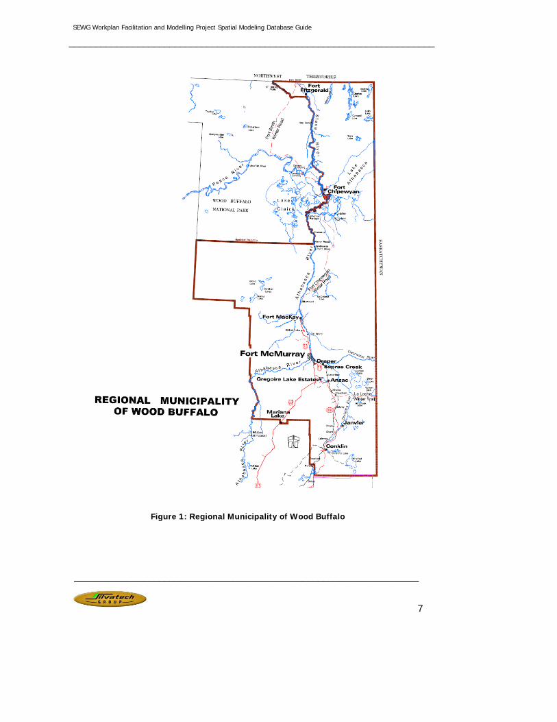
4. Description of the Study Area In September 1998, Alberta Environment announced the creation of the Regional Sustainable Development Strategy (RSDS) for the Athabasca Oil Sands Region. The RSDS study area is defined by the boundary of the Regional Municipality of Wood Buffalo (RMWB) and is also the boundary used for the development of the TEMF.
Stretching from north central Alberta to the borders of Saskatchewan and the Northwest Territories, The RMWB ranks, by area, among the largest municipalities in North America. It was established April 1, 1995, through amalgamation of the City of Fort McMurray and Improvement District No. 143.
Within its 68,454 square kilometers, the municipality is a region of startling contrasts, encompassing both vast stretches of pristine wilderness and one of the fastest growing industrial communities in Canada. Bolstered by the rich oil sands deposits that underlie the region, the dynamic economy of Wood Buffalo is slated for aggressive growth in the future.1 The RMWB supports an ever-diversifying cosmopolitan population that contributes to the cultural richness of the region. While an indigenous population of Chipewyan and Beaver are native to the Athabasca region, by the 1870s the Cree, Metis and Euro-Canadians also made their homes here. In 2002, more than 58 thousand people called the RMWB region their home.
1 http://www.woodbuffalo.ab.ca/residents/regional_profile/RegionalProfile.pdf
SEWG Workplan Facilitation and Modelling Project Spatial Modeling Database Guide
_____________________________________________________________________
_________________________________________________________________
7
Figure 1: Regional Municipality of Wood Buffalo

SEWG Workplan Facilitation and Modelling Project Spatial Modeling Database Guide
_____________________________________________________________________
_________________________________________________________________
8
5. Landbase Inventories Landscape simulation models require spatial data to define the study area and its composition as well as any zones of activity where specific management requirements will be simulated. Both spatially stratified and explicit simulation
models require the generation of a GIS file commonly referred to as a “resultant” that is the product of an overlay process. The process involves combining separate spatial datasets (points, lines or polygons) to create a new output vector dataset. The overlay process can be thought of in a similar way to mathematical Venn diagram overlays. Figure 2 shows how spatial data layer A-B is overlaid onto spatial data layer 1-2 and the “result” is the final coverage that includes the attributes of both data sets.
Two separate resultant files will be created for the Main Program modelling component of this project. The first resultant, the ALCES resultant, will enable the aggregation of all the study area into the appropriate canisters for
input into the ALCES model. The second resultant file, the spatial resultant will be created by overlaying additional spatial layers to the ALCES resultant in order to enable the spatial simulation of anthropogenic and natural disturbance scenarios.
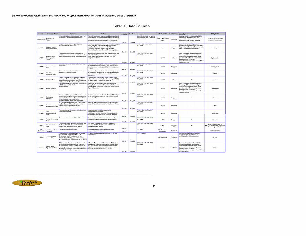
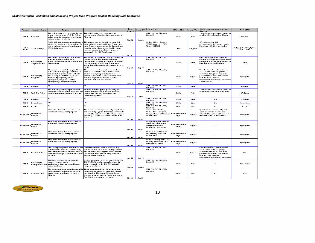
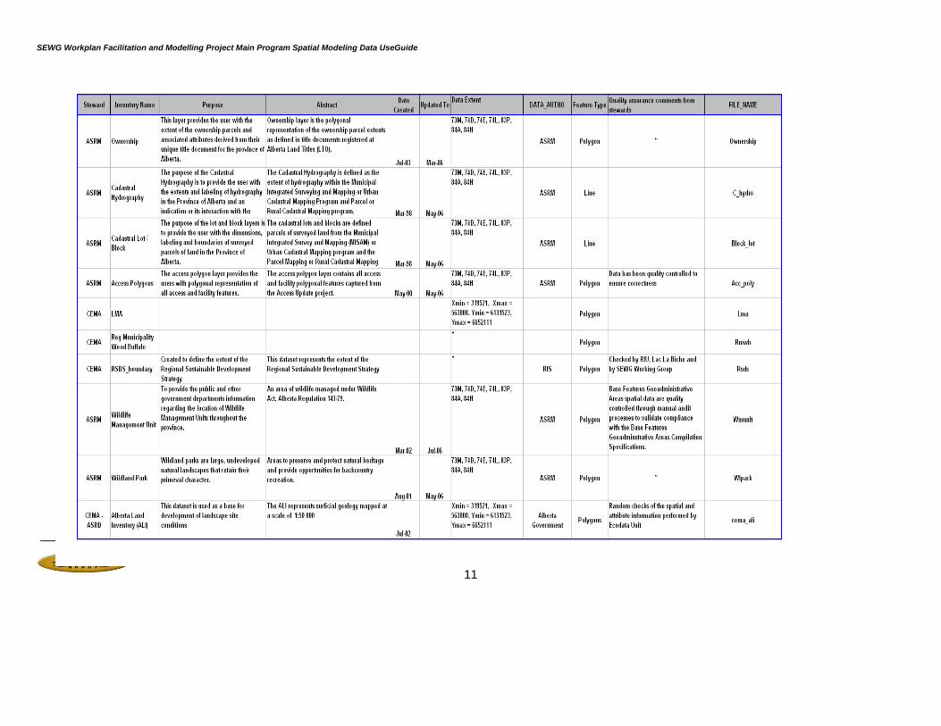
The table below shows a summary of the inventory layers received from SEWG for the modelling that were used to stratify the study area into the necessary categories for input into the ALCES model.
Figure 2: Overlay Process
SEWG Workplan Facilitation and Modelling Project Main Program Spatial Modeling Data UseGuide
________________________________________________________________
9
Table 1: Data Sources
SEWG Workplan Facilitation and Modelling Project Main Program Spatial Modeling Data UseGuide
________________________________________________________________
10
SEWG Workplan Facilitation and Modelling Project Main Program Spatial Modeling Data UseGuide
________________________________________________________________
11

SEWG Workplan Facilitation and Modelling Project Main Program Spatial Modeling Data UseGuide
________________________________________________________________
12
Additional layers were added to the ALCES resultant for the spatial modelling and the additional layers are shown below.
Steward Inventory Name Abstract
Silvatech 1/4 township grid Basis for generic bitumen extraction spatial simulation
ACC caribou range Habitat ranges used to evaluate impacts on caribou habitat
SEWG golder sceanrio Projection to 2010 used as the starting point for time 0 status of surface mine activity in simulation modelling
ALPAC spatial harvest blocks Spatial harvest sequence provided by Alberta Pacific Forest Industries Ltd.
Silvatech SAGD Footprint Spatial representation of generic in-situ bitumen extraction play.
Silvatech Surface Mine Footprint Spatial representation of generic surface mine bitumen extraction play.
First Nations TLU Traditional Land Use Areas
ALPAC THLB Timber havesting land base delineation
The Oil Sands Area Section of the EUB’s Geology and
Reserves Group Bitumen Pay
Used to determine spatial bitumen extraction land base and sequencing: <15m uneconomic, 15-25 thin, >25 thick. Bitumen Pay Thickness (thickness of deposit not depth to deposit) where bitumen is assumed to compose >50% of the deposit. This information was provided solely for use by Silvitech on behalf of SEWG, and the EUB has requested that any distribution of the data be limited to CEMA members only.
Silvatech Fire Spatial fire sequnece generated using MapNow
ALPAC FMA Boundary Alberta Pacific Forest Industries Ltd. FMA boundary
Table 2: Additional layers for spatial resultant

SEWG Workplan Facilitation and Modelling Project Main Program Spatial Modeling Data UseGuide
_________________________________________________________________
13
5.1. Forest Cover Inventory Available forest inventory data varies in quality and resolution significantly across the study area. Forest cover data is a mandatory requirement for forest landscape simulation models and as such influences the modelling approaches, assumptions and interpretation of results possible. Because of the variability and the importance of this data, a separate section regarding just this component is included here.
5.1.1. Alberta Vegetation Inventory The Alberta Vegetation Inventory (AVI) is a photo-based digital inventory developed to identify the type, extent and conditions of vegetation, where it exists and what changes are occurring. AVI polygons have the following attributes:
• Moisture Regime
• Crown Closure
• Stand Height
• Species Composition and Percentage
• Stand Structure and Value
• Stand Origin
• Timber Productivity Rating
• Interpreters Initials
• Naturally Non-Forested Vegetated Land (i.e. shrubs, forbs)
• Naturally Non-Vegetated Land (i.e. rivers, rock barren)
• Anthropogenic Vegetated Land (i.e. agriculture, industrial)
• Anthropogenic Non-Vegetated Land (i.e. created by man)
• Stand Modifier, Extent and Year (i.e. burn, clearcut)
• Data Source
The AVI is considered to be a very accurate vegetation inventory and five audits are required when approving Crown managed AVI data:
• Photo interpretation audit - acceptance accuracy 80%.
• Fieldwork audit - work reviewed but no acceptance accuracy specified.
• Orthophoto base transfer audit - acceptance accuracy 90%.
• Attribute coding audit - acceptance accuracy 95%.
• Digital attribute database audit - acceptance accuracy 100%.

SEWG Workplan Facilitation and Modelling Project Main Program Spatial Modeling Data UseGuide
_________________________________________________________________
14
Figure 3: Sample Alberta Vegetation Inventory Map - Scale = 1 Township
Alberta Pacific Forest Industries Ltd. has generated Alberta Vegetation Inventory standard data in support of their Forest Management Agreement and this covered approximately 48 of the study area.
5.1.2. The Alberta Ground Cover Classification Inventory The Alberta Ground Cover Classification (AGCC) is derived using Landsat TM and 7 ETM imagery to create a land-use / land cover map of the province. This information was primarily intended to support the Forest Protection Division of Alberta Sustainable Resource Development (ASRD) forest fuels data set.
SEWG Workplan Facilitation and Modelling Project Main Program Spatial Modeling Data UseGuide
_________________________________________________________________
15
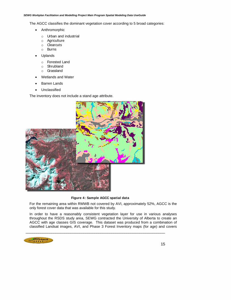
The AGCC classifies the dominant vegetation cover according to 5 broad categories:
• Anthromorphic
o Urban and industrial o Agriculture o Clearcuts o Burns
• Uplands
o Forested Land o Shrubland o Grassland
• Wetlands and Water
• Barren Lands
• Unclassified
The inventory does not include a stand age attribute.
Figure 4: Sample AGCC spatial data
For the remaining area within RMWB not covered by AVI, approximately 52%, AGCC is the only forest cover data that was available for this study.
In order to have a reasonably consistent vegetation layer for use in various analyses throughout the RSDS study area, SEWG contracted the University of Alberta to create an AGCC with age classes GIS coverage. This dataset was produced from a combination of classified Landsat images, AVI, and Phase 3 Forest Inventory maps (for age) and covers
SEWG Workplan Facilitation and Modelling Project Main Program Spatial Modeling Data UseGuide
_________________________________________________________________
16
approximately 35% of the study area. The Phase 3 Forest Inventory was created from 1970-1986 by manually classifying black and white 1:15 000 aerial photography.
In January 2005, the Strategic Corporate Services Division of the Resource Information Management Branch of Alberta Sustainable Resource Development undertook an audit of a portion of this inventory in order to assess the certainty with which it could be used in strategic or operational planning exercises. The audit included the review of 24 townships, roughly 224,000 hectares, within forest management units A6, A9, A10, A11 and A12.
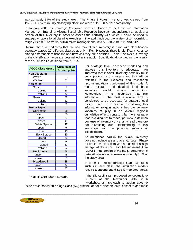
Overall, the audit indicates that the accuracy of this inventory is poor, with classification accuracy across 27 different classes at only 45%. However, there is significant variance among different classifications and how well they are classified. Table 3 shows a summary of the classification accuracy determined in the audit. Specific details regarding the results of the audit can be obtained from ASRD.
For strategic level landscape modelling and analysis, this inventory is adequate. An improved forest cover inventory certainly must be a priority for this region and this will be reflected in the research and monitoring recommendations component of this study. A more accurate and detailed land base inventory would reduce uncertainty. Nonetheless, it is recognized that this information is the best available and is considered to be adequate for strategic level assessments. It is certain that utilizing this information to gain insights into the dynamic variables at play in an overall regional cumulative effects context is far more valuable than deciding not to model potential outcomes because of inventory uncertainty and therefore not advancing our understanding of this landscape and the potential impacts of development.
As mentioned earlier, the AGCC inventory does not include a stand age attribute. Phase 3 Forest Inventory data was not used to assign an age attribute for Land Management Area (LMA) 1 - the portion of the study area north of Lake Athabasca – representing roughly 17% of the study area.
In order to project forested stand attributes such as seral class, the simulation models require a starting stand age for forested areas.
The Silvatech Team proposed conceptually to SEWG at the November 28th, 2006 workshop, an approach to assign ages to
these areas based on an age class (AC) distribution for a sizeable area closest to and most
AGCC Class Group Classification Accuracy (%)
Non-vegetatedWater 93Wetland 83
Non-forestShrub 59
Upland 36wetland 49
Grass 48Upland 31wetland 56
Forest TypesConiferous 88
Pine 53open 47closed 41
White Spruce 17open 0closed 16
Black Spruce 80upland 56
open 0closed 51
wetland 72Deciduous 82
open 0closed 80
Mixedwood 38open 47closed 33
Table 3: AGCC Audit Results
SEWG Workplan Facilitation and Modelling Project Main Program Spatial Modeling Data UseGuide
_________________________________________________________________
17
ecologically similar to LMA 1. At that time, it was assumed that LMA 2 (directly south of the lake) most closely resembles LMA1 in terms of its ecology, natural disturbance history and relative absence of anthropogenic disturbance. In principle, SEWG approved this approach as reasonable and rational.
The approach proposed was simply to determine the current forested age class distribution of LMA2 by ALCES Landscape Type (LT) and use this ratio to proportionately assign ages to the forested LT’s in LMA1. Within each LT, the actual distribution of age assignments to individual polygons would be done randomly to minimize bias.
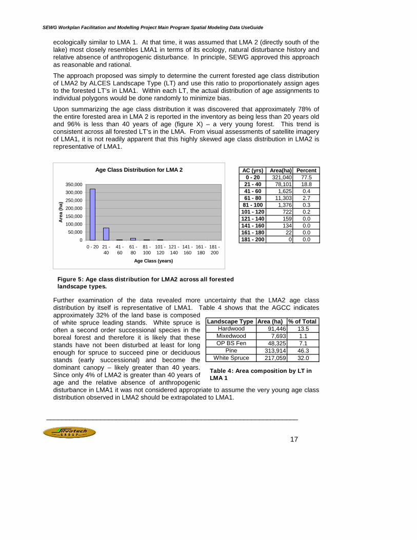
Upon summarizing the age class distribution it was discovered that approximately 78% of the entire forested area in LMA 2 is reported in the inventory as being less than 20 years old and 96% is less than 40 years of age (figure X) – a very young forest. This trend is consistent across all forested LT’s in the LMA. From visual assessments of satellite imagery of LMA1, it is not readily apparent that this highly skewed age class distribution in LMA2 is representative of LMA1.
Further examination of the data revealed more uncertainty that the LMA2 age class distribution by itself is representative of LMA1. Table 4 shows that the AGCC indicates approximately 32% of the land base is composed of white spruce leading stands. White spruce is often a second order successional species in the boreal forest and therefore it is likely that these stands have not been disturbed at least for long enough for spruce to succeed pine or deciduous stands (early successional) and become the dominant canopy – likely greater than 40 years. Since only 4% of LMA2 is greater than 40 years of age and the relative absence of anthropogenic disturbance in LMA1 it was not considered appropriate to assume the very young age class distribution observed in LMA2 should be extrapolated to LMA1.
Figure 5: Age class distribution for LMA2 across all forested landscape types.
Age Class Distribution for LMA 2
0
50,000
100,000
150,000
200,000
250,000
300,000
350,000
0 - 20 21 -40
41 -60
61 -80
81 -100
101 -120
121 -140
141 -160
161 -180
181 -200
Age Class (years)
Are
a (h
a)
AC (yrs) Area(ha) Percent0 - 20 321,040 77.521 - 40 78,101 18.841 - 60 1,625 0.461 - 80 11,303 2.781 - 100 1,376 0.3101 - 120 722 0.2121 - 140 159 0.0141 - 160 134 0.0161 - 180 22 0.0181 - 200 0 0.0
Table 4: Area composition by LT in LMA 1
Landscape Type Area (ha) % of TotalHardwood 91,446 13.5Mixedwood 7,693 1.1OP BS Fen 48,325 7.1
Pine 313,914 46.3White Spruce 217,059 32.0
SEWG Workplan Facilitation and Modelling Project Main Program Spatial Modeling Data UseGuide
_________________________________________________________________
18
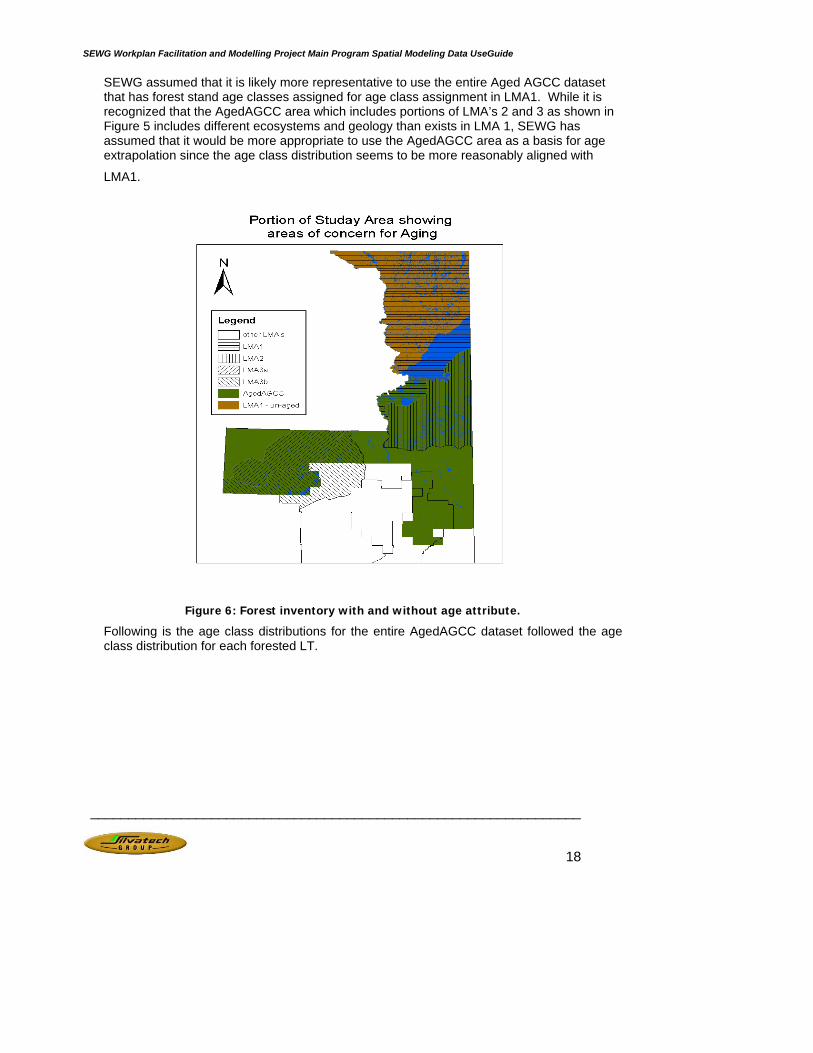
SEWG assumed that it is likely more representative to use the entire Aged AGCC dataset that has forest stand age classes assigned for age class assignment in LMA1. While it is recognized that the AgedAGCC area which includes portions of LMA’s 2 and 3 as shown in Figure 5 includes different ecosystems and geology than exists in LMA 1, SEWG has assumed that it would be more appropriate to use the AgedAGCC area as a basis for age extrapolation since the age class distribution seems to be more reasonably aligned with
LMA1.
Figure 6: Forest inventory with and without age attribute.
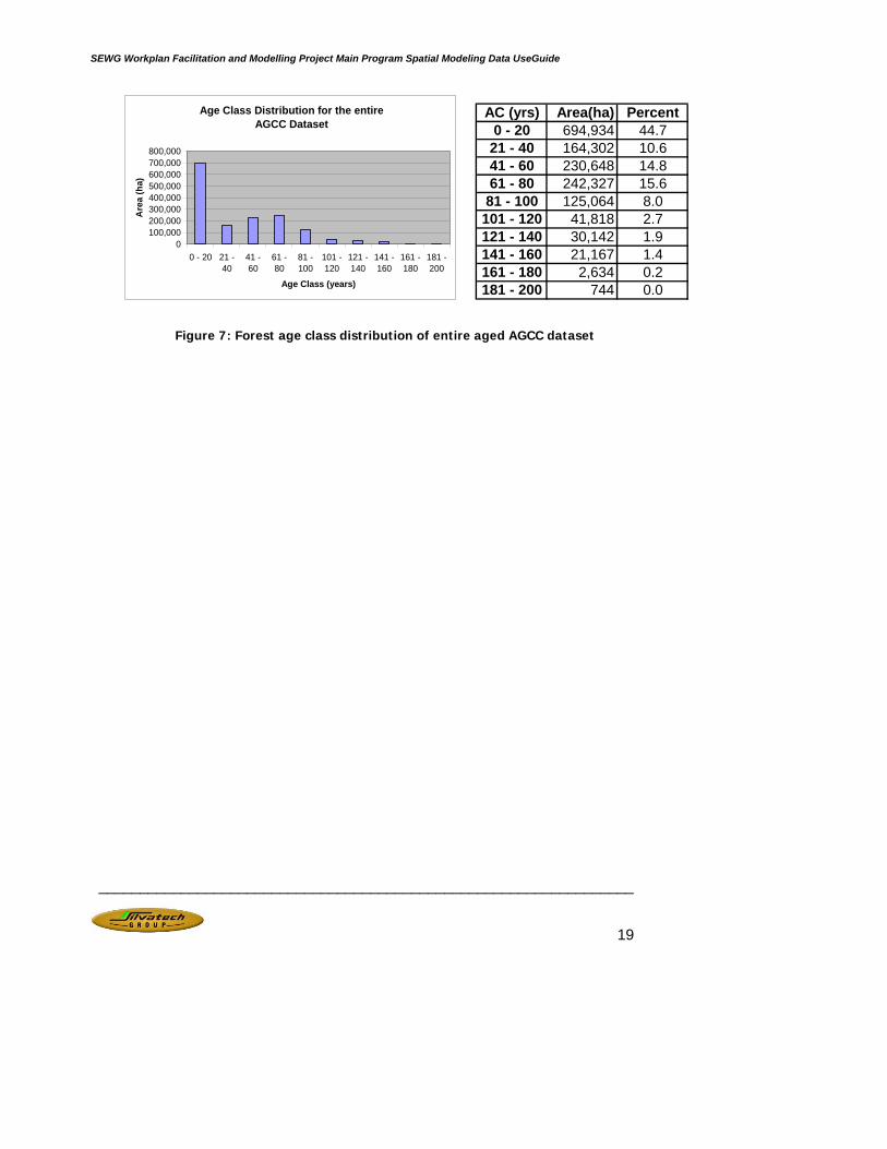
Following is the age class distributions for the entire AgedAGCC dataset followed the age class distribution for each forested LT.
SEWG Workplan Facilitation and Modelling Project Main Program Spatial Modeling Data UseGuide
_________________________________________________________________
19
Age Class Distribution for the entire AGCC Dataset
0100,000200,000300,000400,000500,000600,000700,000800,000
0 - 20 21 -40
41 -60
61 -80
81 -100
101 -120
121 -140
141 -160
161 -180
181 -200
Age Class (years)
Are
a (h
a)
Figure 7: Forest age class distribution of entire aged AGCC dataset
AC (yrs) Area(ha) Percent0 - 20 694,934 44.7
21 - 40 164,302 10.641 - 60 230,648 14.861 - 80 242,327 15.681 - 100 125,064 8.0
101 - 120 41,818 2.7121 - 140 30,142 1.9141 - 160 21,167 1.4161 - 180 2,634 0.2181 - 200 744 0.0

SEWG Workplan Facilitation and Modelling Project Main Program Spatial Modeling Data UseGuide
_________________________________________________________________
20
Age Class Distribution of 'Cl BS Forest' LT
0
1,000
2,000
3,000
4,000
5,000
6,000
0 - 20 21 -40
41 -60
61 -80
81 -100
101 -120
121 -140
141 -160
161 -180
181 -200
Age Class (years)
Are
a (h
a)
Figure 8: Forest age class distribution of Closed Black Spruce Forest
Figure 9: Forest age class distribution of Hardwood
Age Class Distribution of 'Hardwood' LT
05,000
10,00015,00020,00025,00030,00035,00040,00045,000
0 - 20 21 -40
41 -60
61 -80
81 -100
101 -120
121 -140
141 -160
161 -180
181 -200
Age Class (years)
Are
a (h
a)AC (yrs) Area(ha) Percent
0 - 20 2,705 13.421 - 40 144 0.741 - 60 2,240 11.161 - 80 5,666 28.1
81 - 100 3,750 18.6101 - 120 1,570 7.8121 - 140 3,222 16.0141 - 160 791 3.9161 - 180 66 0.3181 - 200 3 0.0
AC (yrs) Area(ha) Percent0 - 20 12,779 16.521 - 40 999 1.341 - 60 7,928 10.261 - 80 39,956 51.5
81 - 100 7,866 10.1101 - 120 5,121 6.6121 - 140 1,515 2.0141 - 160 1,295 1.7161 - 180 93 0.1181 - 200 69 0.1
Age Class Distribution of 'Mixedwood' LT
0
10,000
20,000
30,000
40,000
50,000
60,000
0 - 20 21 -40
41 -60
61 -80
81 -100
101 -120
121 -140
141 -160
161 -180
181 -200
Age Class (years)
Are
a (h
a)
AC (yrs) Area(ha) Percent0 - 20 49,519 36.021 - 40 10,027 7.341 - 60 9,491 6.961 - 80 28,122 20.4
81 - 100 15,376 11.2101 - 120 7,208 5.2121 - 140 7,323 5.3141 - 160 9,340 6.8161 - 180 1,216 0.9181 - 200 63 0.0
Figure 10: Forest age class distribution of Mixedwood

SEWG Workplan Facilitation and Modelling Project Main Program Spatial Modeling Data UseGuide
_________________________________________________________________
21
Age Class Distribution of 'Pine' LT
050,000
100,000150,000200,000250,000300,000350,000400,000450,000500,000
0 - 20 21 -40
41 -60
61 -80
81 -100
101 -120
121 -140
141 -160
161 -180
181 -200
Age Class (years)
Are
a (h
a)
Age Class Distribution of 'White Spruce' LT
0
5,000
10,000
15,000
20,000
25,000
30,000
0 - 20 21 -40
41 -60
61 -80
81 -100
101 -120
121 -140
141 -160
161 -180
181 -200
Age Class (years)
Are
a (h
a)Age Class Distribution of 'OP BS Fen' LT
020,00040,00060,00080,000
100,000120,000140,000160,000180,000200,000
0 - 20 21 -40
41 -60
61 -80
81 -100
101 -120
121 -140
141 -160
161 -180
181 -200
Age Class (years)
Are
a (h
a)AC (yrs) Area(ha) Percent
0 - 20 173,801 30.521 - 40 61,819 10.841 - 60 178,506 31.361 - 80 76,398 13.481 - 100 53,467 9.4101 - 120 11,325 2.0121 - 140 9,174 1.6141 - 160 4,550 0.8161 - 180 593 0.1181 - 200 230 0.0
AC (yrs) Area(ha) Percent0 - 20 443,497 67.021 - 40 89,500 13.541 - 60 19,563 3.061 - 80 66,022 10.081 - 100 26,236 4.0101 - 120 9,059 1.4121 - 140 5,191 0.8141 - 160 2,585 0.4161 - 180 374 0.1181 - 200 303 0.0
AC Area(ha) Percent0 - 20 12,634 14.7
21 - 40 1,812 2.141 - 60 12,920 15.061 - 80 26,163 30.481 - 100 18,368 21.3101 - 120 7,535 8.7121 - 140 3,715 4.3141 - 160 2,606 3.0161 - 180 291 0.3181 - 200 77 0.1
Figure 11: Forest age class distribution of Bog Fen
Figure 12: Forest age class distribution of Pine
Figure 13: Forest age class distribution of White Spruce

SEWG Workplan Facilitation and Modelling Project Main Program Spatial Modeling Data UseGuide
_________________________________________________________________
22
While it is not known for certain if this age class distribution is a better representation of the age class distribution in LMA1 than that of just LMA2 without an inventory audit that includes ground sampling, the distributions observed are more normalized and as such are considered to be a more reasonable basis upon which to make the data extrapolation.
Following are the broad steps used to assign ages in LMA 1 according to the age class distribution observed in the AgedAGCC dataset.
• The proportion of each LT that is within each age class is first determined. These will become the targets when assigning age classes to forested LT’s in LMA 1.
• To ensure that the aging of forested LT’s is random (and not east to west in a youngest to oldest manner for example), a random seed value is applied to every forested LT polygon in LMA 1.
• The age classes will be assigned according to the age class distribution for each LT rather than across the entire landscape at once to capture species variance and therefore the seed values will be randomly applied to each LT individually.
• For each LT, the inventory table will be sorted by the random seed value and then ages will be assigned from youngest to oldest according to the order of the seed value. This is intended to ensure that stands within each age class will exist in a spatially random arrangement across the landscape.
• A map of age classes assigned for each LT will be produced to verify the random distribution across the landscape.
Formatted: Bullets andNumbering
SEWG Workplan Facilitation and Modelling Project Main Program Spatial Modeling Data UseGuide
_________________________________________________________________
23
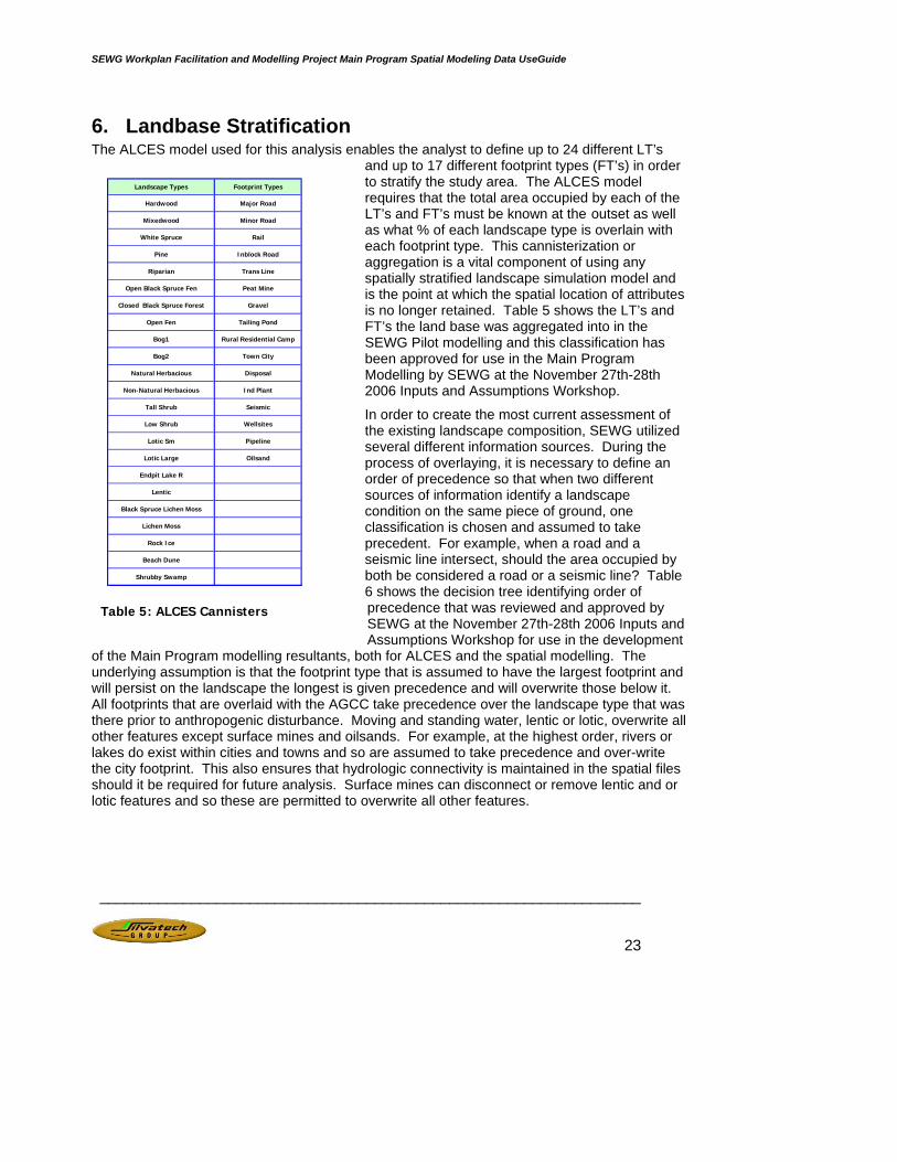
6. Landbase Stratification The ALCES model used for this analysis enables the analyst to define up to 24 different LT’s
and up to 17 different footprint types (FT’s) in order to stratify the study area. The ALCES model requires that the total area occupied by each of the LT’s and FT’s must be known at the outset as well as what % of each landscape type is overlain with each footprint type. This cannisterization or aggregation is a vital component of using any spatially stratified landscape simulation model and is the point at which the spatial location of attributes is no longer retained. Table 5 shows the LT’s and FT’s the land base was aggregated into in the SEWG Pilot modelling and this classification has been approved for use in the Main Program Modelling by SEWG at the November 27th-28th 2006 Inputs and Assumptions Workshop.
In order to create the most current assessment of the existing landscape composition, SEWG utilized several different information sources. During the process of overlaying, it is necessary to define an order of precedence so that when two different sources of information identify a landscape condition on the same piece of ground, one classification is chosen and assumed to take precedent. For example, when a road and a seismic line intersect, should the area occupied by both be considered a road or a seismic line? Table 6 shows the decision tree identifying order of precedence that was reviewed and approved by SEWG at the November 27th-28th 2006 Inputs and Assumptions Workshop for use in the development
of the Main Program modelling resultants, both for ALCES and the spatial modelling. The underlying assumption is that the footprint type that is assumed to have the largest footprint and will persist on the landscape the longest is given precedence and will overwrite those below it. All footprints that are overlaid with the AGCC take precedence over the landscape type that was there prior to anthropogenic disturbance. Moving and standing water, lentic or lotic, overwrite all other features except surface mines and oilsands. For example, at the highest order, rivers or lakes do exist within cities and towns and so are assumed to take precedence and over-write the city footprint. This also ensures that hydrologic connectivity is maintained in the spatial files should it be required for future analysis. Surface mines can disconnect or remove lentic and or lotic features and so these are permitted to overwrite all other features.
Landscape Types Footprint Types
Hardwood Major Road
Mixedwood Minor Road
White Spruce Rail
Pine Inblock Road
Riparian Trans Line
Open Black Spruce Fen Peat Mine
Closed Black Spruce Forest Gravel
Open Fen Tailing Pond
Bog1 Rural Residential Camp
Bog2 Town City
Natural Herbacious Disposal
Non-Natural Herbacious Ind Plant
Tall Shrub Seismic
Low Shrub Wellsites
Lotic Sm Pipeline
Lotic Large Oilsand
Endpit Lake R
Lentic
Black Spruce Lichen Moss
Lichen Moss
Rock Ice
Beach Dune
Shrubby Swamp
Table 5: ALCES Cannisters

SEWG Workplan Facilitation and Modelling Project Main Program Spatial Modeling Data UseGuide
_________________________________________________________________
24
Rank Feature Rank Feature1 Surface Mine 16 Black Spruce2 Lentic or Lotic 17 Fen/Bog3 Town / City 18 Hardwood4 Industrial Plant 19 White Spruce5 Rural Residence / Camp / Campground 20 Shrub6 Major Road 21 Rock / Ice7 Minor Road 22 Pine8 Pipeline 23 Mixedwood9 Transline 24 Moss / Lichen
10 Wellsites 25 Natural Herbaceous11 Miscellaneous Facilities 26 Non-Native Herbaceous12 Gravel 27 Open Black Spruce Fen13 Seismic 28 Open Black Spruce / Lichen Moss14 Riparian 29 Open Treeless Fen15 Beach 30 Classify Proportionately
31 Unclassified
Order of Precedance for Overlay Process
Table 6: SEWG Order of Precedence for Current Landscape Condition Overlay Process
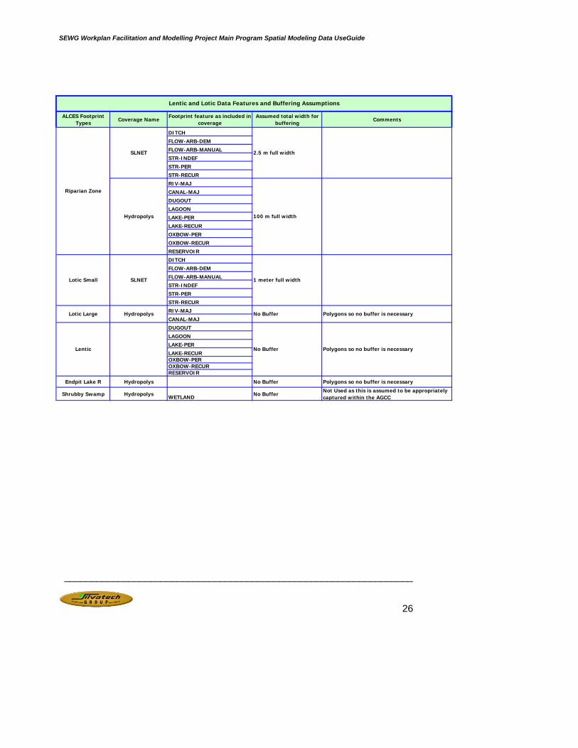
Although many data types are often digitally stored as lines or points, in reality they all are actually polygons with shape and area. These spatial characteristics need to be represented in the resultant file in order to properly account for the area occupied by historic but not reclaimed and current anthropogenic footprint. Therefore, point and line footprint features are buffered and converted to polygons prior to overlay. The following table outlines SEWG’s assumptions for buffering line and point data for input into the resultant file.

SEWG Workplan Facilitation and Modelling Project Main Program Spatial Modeling Data UseGuide
_________________________________________________________________
25
ALCES Footprint Types
Coverage NameFootprint feature as included in
coverageAssumed total width for
bufferingComments
INTERCHANGE-RAMP
ROAD-PAVED-DIV
ROAD-PAVED-UNDIV-2L
ROAD-GRAVEL-2LROAD-GRAVEL-1LROAD-UNCLASSIFIEDROAD-UNIMPROVEDROAD-WINTER-ROADTRUCK-TRAIL
Transmission Lines Powerlines TRANS-LINE 30 m full width Includes Right-of-Way
Gravel Hydropolys QUARRY 300 m diameterNo buffer required. If a point, assume 300m diameter circle polygon. If a polygon, leave as is.
HELIPORT-EVENT 100 m diameter Point data buffered by a 50 m radius
OFFICE WILDFIRE MANAGEMENT
100 m diameter Point data buffered by a 50 m radius
TOWER-LOOKOUT 100 m diameter Point data buffered by a 50 m radius
TOWER-MAJOR 100 m diameter Point data buffered by a 50 m radius
CUTLINE-TRAILCUTLINE TRAIL WITHIN CLEARINGTRAIL-ATV
TRAIL-ATV-INDEFINITE
WELL
WELL-ABAND
WELL-GASWELL-GAS-ABANDWELL-GAS-CAPPEDWELL-OILWELL-OIL-ABANDWELL-WATER 0.5 hectaresWELL-WATER-ABAND 0.5 hectares
Pipelines Pipelines PIPELINE12 m assumed to be area weighted average
Assumed to be an area weighted average
6 m pre 2000; 2.5 m 2000+
There is a significant range in seismic line widths existing on the landbase. These assumptions are assumed to be reasonable for the purposes of SEWG strategic modelling.
WellsitesWells are point data and therefore we are using a radius to buffer
.81 ha for conventional oil and natural gas wellites; 4 ha for SAGD, 0.5 ha for exploratory, .81 for dry wellsites and unknown wells
0.81 hectares
Miscillaneous Facilities
Seismic Lines
Wellsites
Facilities
Cutlines
Current Footprint Overlay Data Features and Buffering Assumptions
Roads
Roads
Major Road
Minor Road
25 m full width
15 m full width
Includes Right-of-Way
Includes Right-of-Way
Table 7: Current Footprint Overlay Buffering Assumptions
SEWG Workplan Facilitation and Modelling Project Main Program Spatial Modeling Data UseGuide
_________________________________________________________________
26
ALCES Footprint Types
Coverage NameFootprint feature as included in
coverageAssumed total width for
bufferingComments
DITCH
FLOW-ARB-DEM
FLOW-ARB-MANUAL
STR-INDEF
STR-PER
STR-RECUR
RIV-MAJ
CANAL-MAJ
DUGOUT
LAGOON
LAKE-PER
LAKE-RECUR
OXBOW-PER
OXBOW-RECUR
RESERVOIR
DITCH
FLOW-ARB-DEM
FLOW-ARB-MANUAL
STR-INDEF
STR-PER
STR-RECUR
RIV-MAJ
CANAL-MAJ
DUGOUT
LAGOON
LAKE-PER
LAKE-RECUROXBOW-PEROXBOW-RECURRESERVOIR
Endpit Lake R Hydropolys No Buffer Polygons so no buffer is necessary
Shrubby Swamp Hydropolys WETLAND No BufferNot Used as this is assumed to be appropriately captured within the AGCC
Lotic Small
Lotic Large
Lentic
Hydropolys
SLNET
Polygons so no buffer is necessary
Polygons so no buffer is necessary
1 meter full width
No Buffer
No Buffer
Lentic and Lotic Data Features and Buffering Assumptions
Riparian Zone
SLNET
Hydropolys 100 m full width
2.5 m full width
SEWG Workplan Facilitation and Modelling Project Main Program Spatial Modeling Data UseGuide
_________________________________________________________________
27
Landbase Aggregation
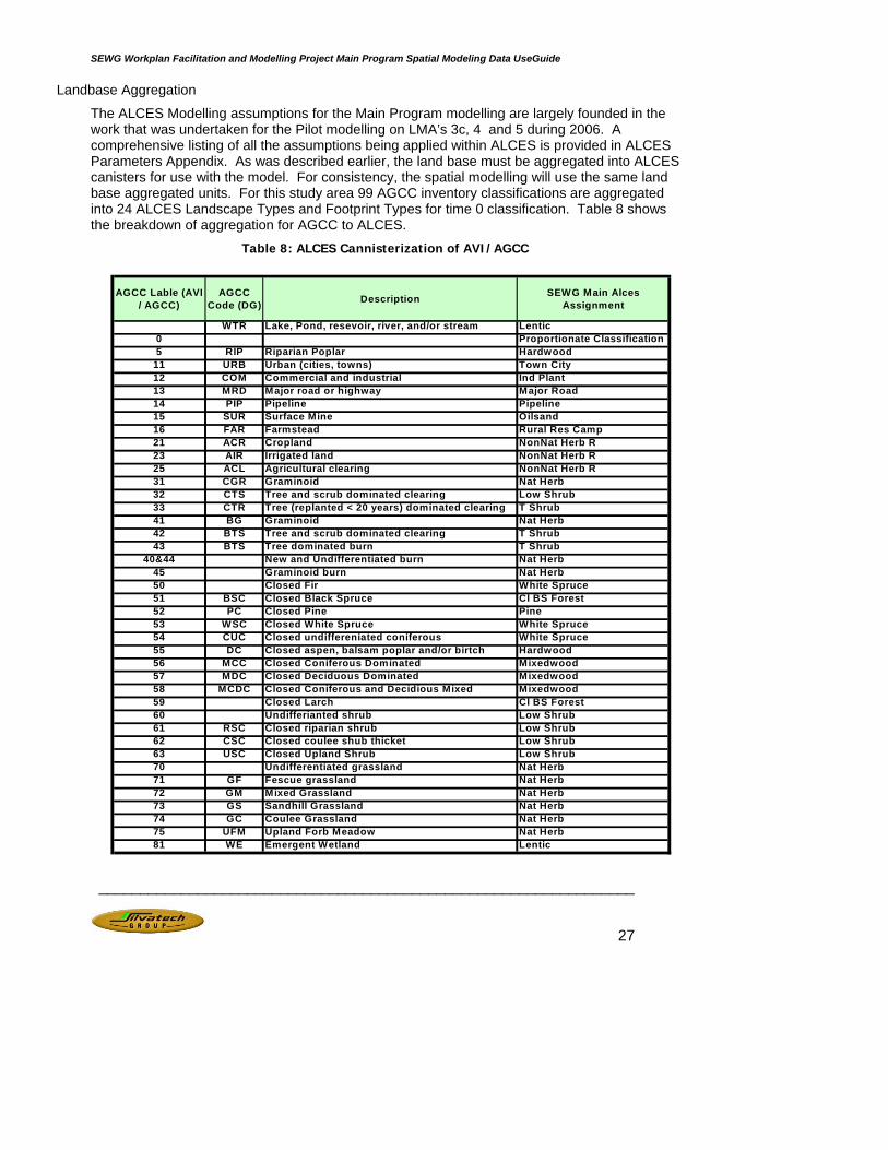
The ALCES Modelling assumptions for the Main Program modelling are largely founded in the work that was undertaken for the Pilot modelling on LMA’s 3c, 4 and 5 during 2006. A comprehensive listing of all the assumptions being applied within ALCES is provided in ALCES Parameters Appendix. As was described earlier, the land base must be aggregated into ALCES canisters for use with the model. For consistency, the spatial modelling will use the same land base aggregated units. For this study area 99 AGCC inventory classifications are aggregated into 24 ALCES Landscape Types and Footprint Types for time 0 classification. Table 8 shows the breakdown of aggregation for AGCC to ALCES.
Table 8: ALCES Cannisterization of AVI/AGCC
AGCC Lable (AVI / AGCC)
AGCC Code (DG) Description SEWG Main Alces
Assignment
WTR Lake, Pond, resevoir, river, and/or stream Lentic0 Proportionate Classification5 RIP Riparian Poplar Hardwood
11 URB Urban (cities, towns) Town City12 COM Commercial and industrial Ind Plant13 MRD Major road or highway Major Road14 PIP Pipeline Pipeline15 SUR Surface Mine Oilsand16 FAR Farmstead Rural Res Camp21 ACR Cropland NonNat Herb R23 AIR Irrigated land NonNat Herb R25 ACL Agricultural clearing NonNat Herb R31 CGR Graminoid Nat Herb32 CTS Tree and scrub dominated clearing Low Shrub33 CTR Tree (replanted < 20 years) dominated clearing T Shrub41 BG Graminoid Nat Herb42 BTS Tree and scrub dominated clearing T Shrub43 BTS Tree dominated burn T Shrub
40&44 New and Undifferentiated burn Nat Herb45 Graminoid burn Nat Herb50 Closed Fir White Spruce51 BSC Closed Black Spruce Cl BS Forest52 PC Closed Pine Pine53 WSC Closed White Spruce White Spruce54 CUC Closed undiffereniated coniferous White Spruce55 DC Closed aspen, balsam poplar and/or birtch Hardwood56 MCC Closed Coniferous Dominated Mixedwood57 MDC Closed Deciduous Dominated Mixedwood58 MCDC Closed Coniferous and Decidious Mixed Mixedwood59 Closed Larch Cl BS Forest60 Undifferianted shrub Low Shrub61 RSC Closed riparian shrub Low Shrub62 CSC Closed coulee shub thicket Low Shrub63 USC Closed Upland Shrub Low Shrub70 Undifferentiated grassland Nat Herb71 GF Fescue grassland Nat Herb72 GM Mixed Grassland Nat Herb73 GS Sandhill Grassland Nat Herb74 GC Coulee Grassland Nat Herb75 UFM Upland Forb Meadow Nat Herb81 WE Emergent Wetland Lentic

SEWG Workplan Facilitation and Modelling Project Main Program Spatial Modeling Data UseGuide
_________________________________________________________________
28

SEWG Workplan Facilitation and Modelling Project Main Program Spatial Modeling Data UseGuide
_________________________________________________________________
29
AGCC Lable (AVI / AGCC)
AGCC Code (DG) Description SEW G M ain Alces
Assignment
82 W G Graminoid W etland Nat Herb83 W SB Shrubby Wetland Bog184 W SB Sphagnum Bog Open Fen85 W OL Lichen Bog Lichen M oss86 W BS Black Spruce Bog (sphagnum Understory) OP BS Fen87 W BL Black Spruce Bog (lichen Understory) BS Lichen M oss88 Undifferentiated wetland Bog189 Open wooded fen Bog190 Open fen Open Fen91 Proportionate Classification
101 BPI Perm ice and snow Rock Ice102 BR Rock, talus, and/or avalanche chute Rock Ice103 BS Exposed Soil Rock Ice104 BAF Alkali flat and/or mud flat Rock Ice105 BUD Upland Dune Rock Ice106 BAD Alluvial Deposit Rock Ice107 BB Beach Beach Dune108 BBL Badland Rock Ice109 BBZ Blowout Zone Rock Ice112 US Cloud, Haze, Shadow Proportionate Classification150 Open Fir W hite Spruce151 BSO Open Black Spruce Cl BS Forest152 PO Open Pine Pine153 W SO Open White Spruce W hite Spruce154 UCO Open undiffereniated coniferous OP BS Fen155 DO Open aspen, balsam poplar and/or birtch Hardwood156 M CO Open Coniferous Dominated M ixedwood157 M DO Open Deciduous Dominated M ixedwood158 M CDO Open Coniferous and Decidious M ixed M ixedwood159 Open Larch BS Lichen M oss161 RSO Open Riparian Shrub Low Shrub162 CSO Open Coulee shrub thicket Low Shrub163 USO Open Upland Shrub Low Shrub164 SO Open Sagebrush Low Shrub831 Open shruby wetland Shrubby Swamp832 Closed shruby wetalnd Shrubby Swamp861 Open Black Spruce / sphagnum bog OP BS Fen862 Closed Black Spruce / sphagnum bog Cl BS Forest891 Open wooded fen Open Fen892 Closed wooded fen Cl BS Forest
5450 Closed Fb Leads Conifer W hite Spruce5451 Closed Sb Leads Conifer Cl BS Forest5452 Closed Pine Leads Conifer Pine5453 Closed Sw Leads Conifer W hite Spruce5459 Leading Larch Cl BS Forest5650 Closed Fb dominated M ixedwood M ixedwood5651 Closed Sb dominated M ixedwood M ixedwood5652 Closed Pine dominated M ixedwood M ixedwood5653 Closed Sw dominated M ixedwood M ixedwood
154150 Open Fb Leads Conifer W hite Spruce154151 Open Sb Leads Conifer Cl BS Forest154152 Open Pine Leads Conifer Pine154153 Open Sw Leads Conifer W hite Spruce154159 Open Leading W hite Spruce W hite Spruce156151 Open Sb dominated M ixedwood M ixedwood156152 Open Pine dominated M ixedwood M ixedwood156153 Open Sw dominated M ixedwood M ixedwood

SEWG Workplan Facilitation and Modelling Project Main Program Spatial Modeling Data UseGuide
_________________________________________________________________
30
7. Landscape Disturbance
7.1. The Spatial Disturbance Queue Sequential simulation models require a rule set or sequence of events to simulate and project change. The spatial model requires a schedule of disturbances according to a range of spatial and temporal objectives. Silviculture systems and stand growth and yields are assigned to each polygon. At each time step, polygons are first ranked according to a disturbance priority. Polygons are then disturbed (denuded) according to the queue subject to meeting any constraints imposed to meet forest level objectives. Polygons are disturbed until a constraint becomes binding, the queue is exhausted or the periodic target is met. At this stage the forest is aged to the next time period, and the process is repeated. At each time period, the model reports the status of every polygon in the landscape. These periodic inventories can then be displayed in maps assess landscape patterns.
For this study, the following overall hierarchy will define the spatial disturbance queue in each time step:
1. Forest Fires
2. Surface mine development and salvage logging
3. In Situ development and salvage logging
4. Forest Harvesting
7.2. Forest Fire It is understood that natural disturbance in the form of fire in the RMWB will alter the age class distribution of the forested landscape. Many of the sub-models being utilized for this study have been developed with the assumption that fire is an active disturbance agent on the environment. Despite human intervention in the form of fire suppression, fire remains a significant disturbance in the RMWB. Dave Andison of Bandaloop computed the 80 year fire cycle (1.25% burned annually) used in the ALCES modelling and this assumes approximately 75% fire suppression is occurring.
SEWG has identified that if the ALCES modelling includes fire but the spatial modelling does not, there could be a significant discrepancy in the modelling results and that this would come about only as an inappropriate artifact of the modelling approaches.
In light of this, Silvatech researched opportunities to incorporate fire modelling spatially in the spatial platform for the SEWG project. Silvatech discussed the approach with modelling peers and reviewed several extension reports summarizing various modelling approaches for incorporating natural disturbance.
In order to maintain consistency in models to the greatest extent possible, SEWG has assumed that fire metrics will be derived in the ALCES model in the form of area burned by landscape type by period, across the entire RMWB study area in the simulations. Over the entire study area this amounts to an average1.25% of each Landscape Type simulated to burn in each year of the projection timeline.
Silvatech research indicates that the rate of burn, severity of burn and burn pattern are the three most important characteristics of fire on habitat and biodiversity (Bergeron et al. 2002).

SEWG Workplan Facilitation and Modelling Project Main Program Spatial Modeling Data UseGuide
_________________________________________________________________
31
The burn rate determines how much fire occurs on the landscape over time. The burn severity determines the effect of fire upon the stand, such as how many trees are killed and which residual structures remain. The burn pattern influences the patches that result after fire (Davis and Boyland 2003).
For strategic level spatial habitat and biodiversity planning as well as timber supply analysis using a spatial platform, Davis and Boyland note that “Burn rate, severity and pattern parameters are both uncertain and stochastic, making modelling fire disturbance deceptively difficult. Parameter uncertainty directly reduces the confidence in model results. However, even if parameters were known with certainty, stochasticity forces model results to include a range of possible futures corresponding to the different pathways of fire disturbance. Very complex patterns occur on the landscape when burn rate, severity and pattern combine, and a wide range of projected landscape conditions are sometimes equally likely given the level of uncertainty and stochasticity in fire projections. Given the complexity and the uncertainty of measuring fire disturbance parameters, we decided it was pragmatic to simplify the problem. In a global sense, we felt that given the potential for misleading results without including disturbance, some method of including disturbances into timber supply and biodiversity modelling was required, however imperfect the method might be. We considered burn rate to be the most important disturbance parameter.”
Detailed modelling of spatial fire patterns could very well lead to massive volumes of data with very significant levels of uncertainty and likely would not add tremendous value to the exercise. Similarly, while fire severity is known to be an important factor in the development of specific stand characteristics for certain wildlife habitat types, the AGCC is not a stand-level forest inventory and as such we would likely be attempting to model at a resolution beyond the intended use of the data. Davis and Boyland concluded in their assessment that ”a simple burn pattern such as an ellipse would be adequate (Gardner et al. 1999).” This level of complexity is also considered appropriate for the SEWG TEMF modelling.
Three spatial natural disturbance modelling options emerged from the literature that were considered for this project and the deterministic disturbance option was chosen. Conceptually, fire will be simulated as just another disturbance type like logging but occurs according to a deterministic schedule.
Because of the stochastic nature of fire, a range of fires could be simulated on the ground spatially each with equal probability of occurring but with locally different outcomes. This is a recognized limitation of applying fire in a spatially explicit way without undertaking a Monte Carlo approach and simulating a range of probabilities. The spatial Monte Carlo approach is outside the scope of this project. However, because the rate of burn per period by LT is derived from a Monte Carlo approach within ALCES, the actual pattern simulated is assumed to be reflective of a probable level within the range of natural variability.
A new modelling software product developed in Alberta called Map Now (designed for use with ALCES) will be utilized to generate a plausible fire pattern representative of the range of natural variation simulated stochastically within ALCES for the Main Program modelling. In essence, the rate of burn by landscape type by period will be exported from ALCES to the Map Now product that will use a randomized algorithm to identify a plausible burn patterns spatially over the study area. The fire growth algorithm randomly chooses the location to burn within each landscape type until it reach the number of fire patches and area of fire in each landscape type provided by the ALCES output. The algorithm will not necessarily match individual fire size metrics from ALCES since the size of each fire patch is also randomly grown resulting in variable fire sizes and shapes. Fires will be generated in a
SEWG Workplan Facilitation and Modelling Project Main Program Spatial Modeling Data UseGuide
_________________________________________________________________
32
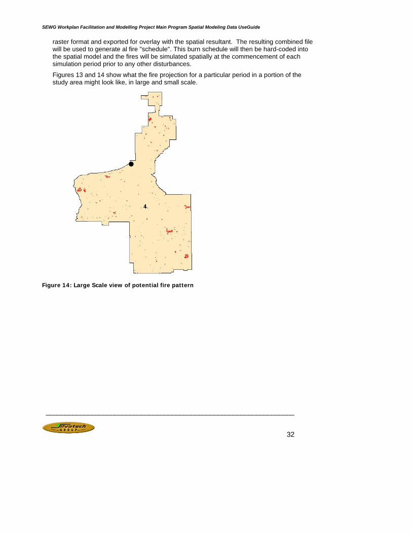
raster format and exported for overlay with the spatial resultant. The resulting combined file will be used to generate al fire "schedule". This burn schedule will then be hard-coded into the spatial model and the fires will be simulated spatially at the commencement of each simulation period prior to any other disturbances.
Figures 13 and 14 show what the fire projection for a particular period in a portion of the study area might look like, in large and small scale.
Figure 14: Large Scale view of potential fire pattern

SEWG Workplan Facilitation and Modelling Project Main Program Spatial Modeling Data UseGuide
_________________________________________________________________
33
Figure 15: Small scale view of potential fire pattern
The actual fire schedule developed will be included in and reported on in the final modelling results.
Table 9: Fire Assumptions Summary
SEWG Workplan Facilitation and Modelling Project Main Program Spatial Modeling Data UseGuide
_________________________________________________________________
34
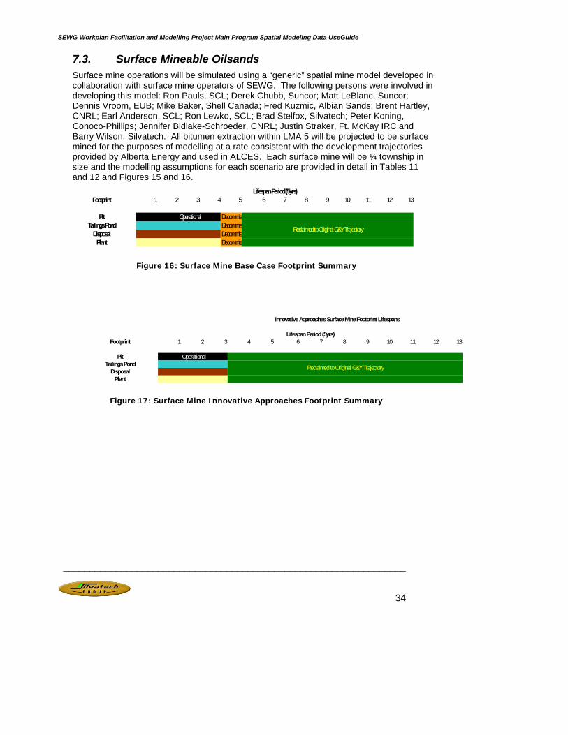
7.3. Surface Mineable Oilsands Surface mine operations will be simulated using a “generic” spatial mine model developed in collaboration with surface mine operators of SEWG. The following persons were involved in developing this model: Ron Pauls, SCL; Derek Chubb, Suncor; Matt LeBlanc, Suncor; Dennis Vroom, EUB; Mike Baker, Shell Canada; Fred Kuzmic, Albian Sands; Brent Hartley, CNRL; Earl Anderson, SCL; Ron Lewko, SCL; Brad Stelfox, Silvatech; Peter Koning, Conoco-Phillips; Jennifer Bidlake-Schroeder, CNRL; Justin Straker, Ft. McKay IRC and Barry Wilson, Silvatech. All bitumen extraction within LMA 5 will be projected to be surface mined for the purposes of modelling at a rate consistent with the development trajectories provided by Alberta Energy and used in ALCES. Each surface mine will be ¼ township in size and the modelling assumptions for each scenario are provided in detail in Tables 11 and 12 and Figures 15 and 16.
Footprint 1 2 3 4 5 6 7 8 9 10 11 12 13
Pit Operational DecommissTailings Pond Decommiss
Disposal DecommissPlant Decommiss
Lifespan Period (5yrs)
Reclaimed to Original G&Y Trajectory
Figure 16: Surface Mine Base Case Footprint Summary
Innovative Approaches Surface Mine Footprint Lifespans
Footprint 1 2 3 4 5 6 7 8 9 10 11 12 13
Pit OperationalTailings Pond
DisposalPlant
Reclaimed to Original G&Y Trajectory
Lifespan Period (5yrs)
Figure 17: Surface Mine Innovative Approaches Footprint Summary
SEWG Workplan Facilitation and Modelling Project Main Program Spatial Modeling Data UseGuide
_________________________________________________________________
35
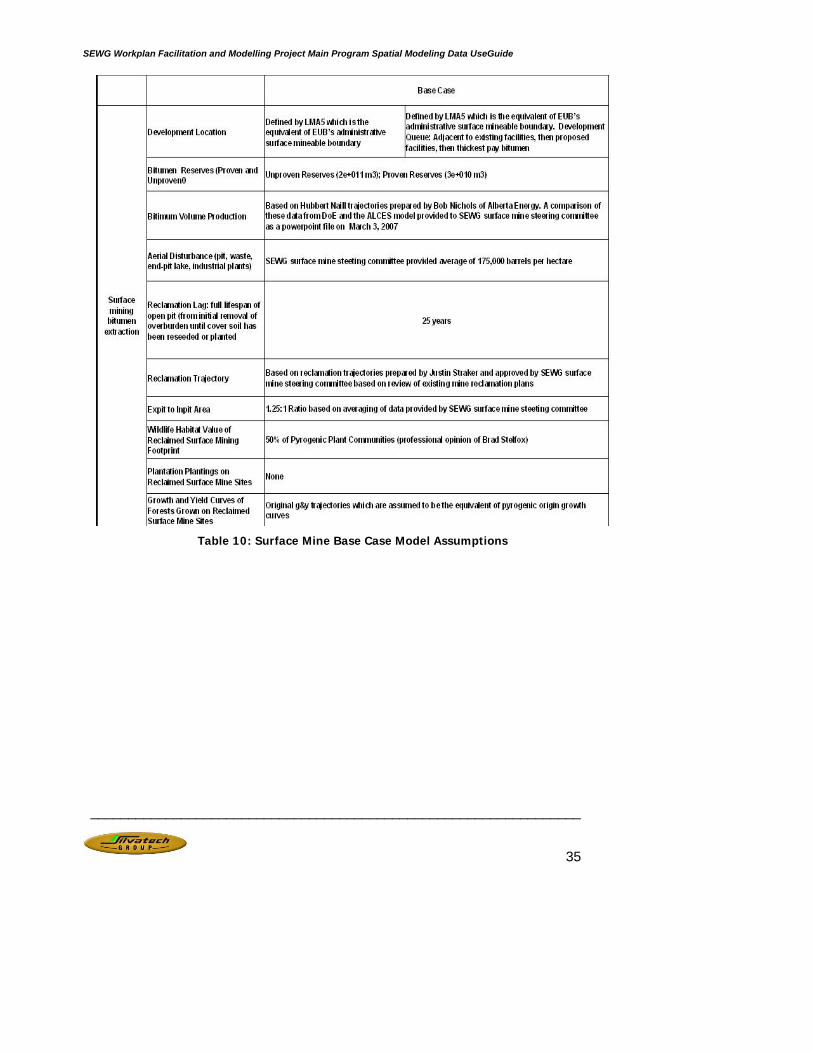
Table 10: Surface Mine Base Case Model Assumptions
SEWG Workplan Facilitation and Modelling Project Main Program Spatial Modeling Data UseGuide
_________________________________________________________________
36
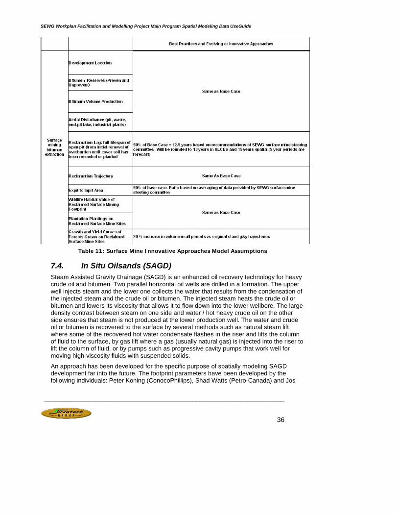
Table 11: Surface Mine Innovative Approaches Model Assumptions
7.4. In Situ Oilsands (SAGD) Steam Assisted Gravity Drainage (SAGD) is an enhanced oil recovery technology for heavy crude oil and bitumen. Two parallel horizontal oil wells are drilled in a formation. The upper well injects steam and the lower one collects the water that results from the condensation of the injected steam and the crude oil or bitumen. The injected steam heats the crude oil or bitumen and lowers its viscosity that allows it to flow down into the lower wellbore. The large density contrast between steam on one side and water / hot heavy crude oil on the other side ensures that steam is not produced at the lower production well. The water and crude oil or bitumen is recovered to the surface by several methods such as natural steam lift where some of the recovered hot water condensate flashes in the riser and lifts the column of fluid to the surface, by gas lift where a gas (usually natural gas) is injected into the riser to lift the column of fluid, or by pumps such as progressive cavity pumps that work well for moving high-viscosity fluids with suspended solids.
An approach has been developed for the specific purpose of spatially modeling SAGD development far into the future. The footprint parameters have been developed by the following individuals: Peter Koning (ConocoPhillips), Shad Watts (Petro-Canada) and Jos

SEWG Workplan Facilitation and Modelling Project Main Program Spatial Modeling Data UseGuide
_________________________________________________________________
37
Lussenburg (JACOS). Barry Wilson and Brad Stelfox (Silvatech) provided the conceptual modeling approach and feedback on the footprint parameters.
Spatial modeling of SAGD is done for Environmental Impact Assessments (EIAs), but only involves the footprints of existing or planned projects. The SEWG work intends to go far beyond that in terms of projected bitumen production. The department of energy has provided SEWG with two key products necessary to support this modeling: 1) a forecast of in-situ production, by year for 100 years, 2) a map of bitumen thickness and locations of existing or planned projects.
The pay zone is a term used to describe the thickness of a bitumen deposit that is considered commercially viable under current economic and technological conditions. The bitumen pay data provided by Alberta Energy for this analysis indicates bitumen pay thickness in meters where bitumen accounts for >50% of the deposit composition. For the purposes of this analysis, a bitumen pay thickness of less than 15m is considered un-economic and is therefore not scheduled for development in the simulations. Thin pay is assumed to be 15 m to 25 m in thickness and thick pay is greater than 25 m in thickness.
Four generic SAGD footprints are proposed:
1. Base Case" in thick bitumen (Thick Pay – Base Case)
2. Base Case in thin bitumen (Thin Pay – Base Case)
Base Case Thick In Situ Footprint Lifespans
# Footprint 1 2 3 4 5 6 7 8 9 10 11 12 13
1 Seismic, delineation, exploration Operational Reclaimed to Original G&Y Trajectory2 Plant, access and pipelines Operational Decommissioned Reclaimed 3 Production wells 1 Operational Decommissioned Reclaimed to Original G&Y Trajectory4 Production wells 2 Operational Decommissioned Reclaimed to Original G&Y Traject5 Production wells 3 Operational Decommissioned Reclaimed
Base Case Thin In Situ Footprint Lifespans
# Footprint 1 2 3 4 5 6 7 8 9 10 11 12 13
1 Seismic, delineation, exploration Operational Reclaimed to Original G&Y Trajectory2 Plant, access and pipelines Operational Decommissioned Reclaimed to Original G&Y Trajectory3 Production wells 1 Operational Decommissioned Reclaimed to Original G&Y Trajectory4 Production wells 2 Operational Decommissioned Reclaimed to Original G&Y Trajectory5 Production wells 3 Operational Decommissioned Reclaimed to Original G&Y Trajectory
Lifespan Period (5yrs)
Lifespan Period (5yrs)
Figure 18: In Situ Base Case Footprint Summary

SEWG Workplan Facilitation and Modelling Project Main Program Spatial Modeling Data UseGuide
_________________________________________________________________
38
Table 12: In Situ Base Case Model Assumptions
3. Innovative Approaches in thick bitumen (Thick Pay – Best Practices)
4. Innovative Approaches in thin bitumen (Thick Pay – Best Practices)
SEWG Workplan Facilitation and Modelling Project Main Program Spatial Modeling Data UseGuide
_________________________________________________________________
39
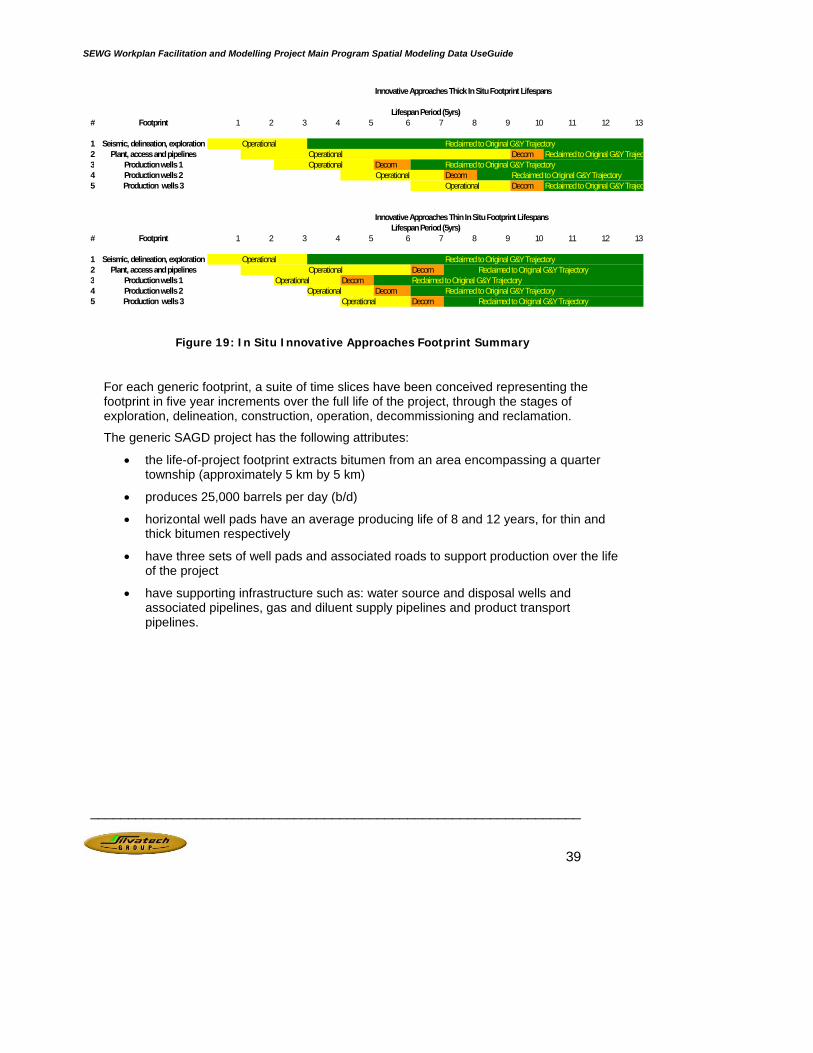
Innovative Approaches Thick In Situ Footprint Lifespans
# Footprint 1 2 3 4 5 6 7 8 9 10 11 12 13
1 Seismic, delineation, exploration Operational Reclaimed to Original G&Y Trajectory2 Plant, access and pipelines Operational Decom Reclaimed to Original G&Y Traject3 Production wells 1 Operational Decom Reclaimed to Original G&Y Trajectory4 Production wells 2 Operational Decom Reclaimed to Original G&Y Trajectory5 Production wells 3 Operational Decom Reclaimed to Original G&Y Traject
Innovative Approaches Thin In Situ Footprint Lifespans
# Footprint 1 2 3 4 5 6 7 8 9 10 11 12 13
1 Seismic, delineation, exploration Operational Reclaimed to Original G&Y Trajectory2 Plant, access and pipelines Operational Decom Reclaimed to Original G&Y Trajectory3 Production wells 1 Operational Decom Reclaimed to Original G&Y Trajectory4 Production wells 2 Operational Decom Reclaimed to Original G&Y Trajectory5 Production wells 3 Operational Decom Reclaimed to Original G&Y Trajectory
Lifespan Period (5yrs)
Lifespan Period (5yrs)
Figure 19: In Situ Innovative Approaches Footprint Summary
For each generic footprint, a suite of time slices have been conceived representing the footprint in five year increments over the full life of the project, through the stages of exploration, delineation, construction, operation, decommissioning and reclamation.
The generic SAGD project has the following attributes:
• the life-of-project footprint extracts bitumen from an area encompassing a quarter township (approximately 5 km by 5 km)
• produces 25,000 barrels per day (b/d)
• horizontal well pads have an average producing life of 8 and 12 years, for thin and thick bitumen respectively
• have three sets of well pads and associated roads to support production over the life of the project
• have supporting infrastructure such as: water source and disposal wells and associated pipelines, gas and diluent supply pipelines and product transport pipelines.
SEWG Workplan Facilitation and Modelling Project Main Program Spatial Modeling Data UseGuide
_________________________________________________________________
40
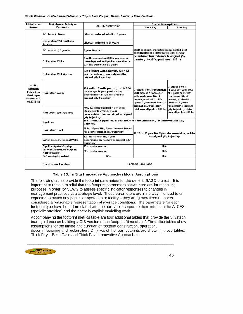
Table 13: In Situ Innovative Approaches Model Assumptions
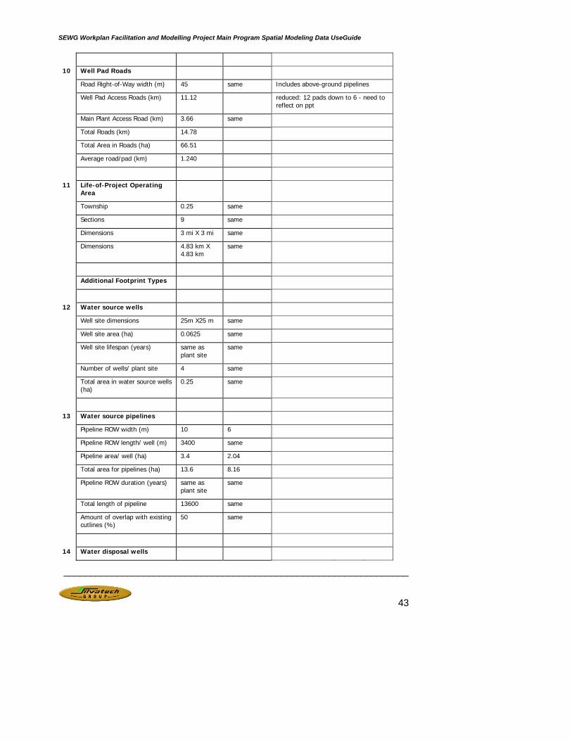
The following tables provide the footprint parameters for the generic SAGD project. It is important to remain mindful that the footprint parameters shown here are for modelling purposes in order for SEWG to assess specific indicator responses to changes in management practices at a strategic level. These parameters are in no way intended to or expected to match any particular operation or facility – they are generalized numbers considered a reasonable representation of average conditions. The parameters for each footprint type have been formulated with the ability to incorporate them into both the ALCES (spatially stratified) and the spatially explicit modelling work.
Accompanying the footprint metrics table are four additional tables that provide the Silvatech team guidance on building a GIS version of the footprint “time slices”. Time slice tables show assumptions for the timing and duration of footprint construction, operation, decommissioning and reclamation. Only two of the four footprints are shown in these tables: Thick Pay – Base Case and Thick Pay – Innovative Approaches.
SEWG Workplan Facilitation and Modelling Project Main Program Spatial Modeling Data UseGuide
_________________________________________________________________
41
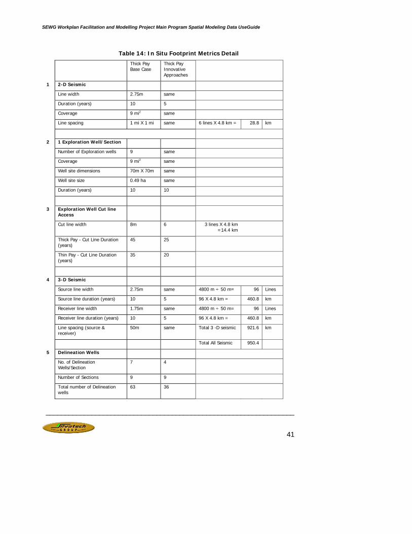
Table 14: In Situ Footprint Metrics Detail
Thick Pay Base Case
Thick Pay Innovative Approaches
1 2-D Seismic
Line width 2.75m same
Duration (years) 10 5
Coverage 9 mi2 same
Line spacing 1 mi X 1 mi same 6 lines X 4.8 km = 28.8 km
2 1 Exploration Well/Section
Number of Exploration wells 9 same
Coverage 9 mi2 same
Well site dimensions 70m X 70m same
Well site size 0.49 ha same
Duration (years) 10 10
3 Exploration Well Cut line Access
Cut line width 8m 6 3 lines X 4.8 km =14.4 km
Thick Pay - Cut Line Duration (years)
45 25
Thin Pay - Cut Line Duration (years)
35 20
4 3-D Seismic
Source line width 2.75m same 4800 m ÷ 50 m= 96 Lines
Source line duration (years) 10 5 96 X 4.8 km = 460.8 km
Receiver line width 1.75m same 4800 m ÷ 50 m= 96 Lines
Receiver line duration (years) 10 5 96 X 4.8 km = 460.8 km
Line spacing (source & receiver)
50m same Total 3 -D seismic 921.6 km
Total All Seismic 950.4
5 Delineation Wells
No. of Delineation Wells/Section
7 4
Number of Sections 9 9
Total number of Delineation wells
63 36
SEWG Workplan Facilitation and Modelling Project Main Program Spatial Modeling Data UseGuide
_________________________________________________________________
42
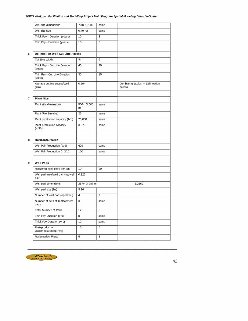
Well site dimensions 70m X 70m same
Well site size 0.49 ha same
Thick Pay - Duration (years) 10 3
Thin Pay - Duration (years) 10 3
6 Delineation Well Cut Line Access
Cut Line width 8m 6
Thick Pay - Cut Line Duration (years)
40 20
Thin Pay - Cut Line Duration (years)
30 15
Average cutline access/well (km)
0.394 Combining Explor. + Delineation access
7 Plant Site
Plant site dimensions 500m X 500 m
same
Plant Site Size (ha) 25 same
Plant production capacity (b/d) 25,000 same
Plant production capacity (m3/d)
3,975 same
8 Horizontal Wells
Well Pair Production (b/d) 629 same
Well Pair Production (m3/d) 100 same
9 Well Pads
Horizontal well pairs per pad 10 20
Well pad area/well pair (ha/well pair)
0.826
Well pad dimensions 287m X 287 m 8.2369
Well pad size (ha) 8.26
Number of well pads operating 4 2
Number of sets of replacement pads
3 same
Total Number of Pads 12 6
Thin Pay Duration (yrs) 8 same
Thick Pay Duration (yrs) 12 same
Post-production Decommissioning (yrs)
15 5
Reclamation Phase 5 5
SEWG Workplan Facilitation and Modelling Project Main Program Spatial Modeling Data UseGuide
_________________________________________________________________
43
10 Well Pad Roads
Road Right-of-Way width (m) 45 same Includes above-ground pipelines
Well Pad Access Roads (km) 11.12 reduced: 12 pads down to 6 - need to reflect on ppt
Main Plant Access Road (km) 3.66 same
Total Roads (km) 14.78
Total Area in Roads (ha) 66.51
Average road/pad (km) 1.240
11 Life-of-Project Operating Area
Township 0.25 same
Sections 9 same
Dimensions 3 mi X 3 mi same
Dimensions 4.83 km X 4.83 km
same
Additional Footprint Types
12 Water source wells
Well site dimensions 25m X25 m same
Well site area (ha) 0.0625 same
Well site lifespan (years) same as plant site
same
Number of wells/ plant site 4 same
Total area in water source wells (ha)
0.25 same
13 Water source pipelines
Pipeline ROW width (m) 10 6
Pipeline ROW length/ well (m) 3400 same
Pipeline area/ well (ha) 3.4 2.04
Total area for pipelines (ha) 13.6 8.16
Pipeline ROW duration (years) same as plant site
same
Total length of pipeline 13600 same
Amount of overlap with existing cutlines (%)
50 same
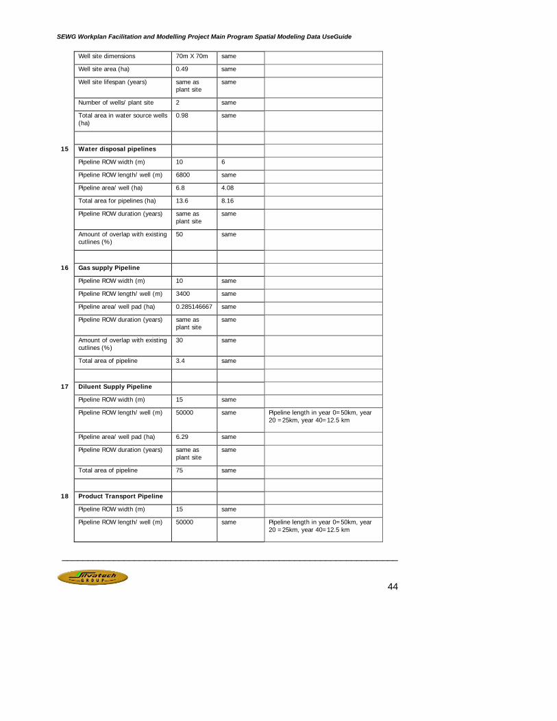
14 Water disposal wells
SEWG Workplan Facilitation and Modelling Project Main Program Spatial Modeling Data UseGuide
_________________________________________________________________
44
Well site dimensions 70m X 70m same
Well site area (ha) 0.49 same
Well site lifespan (years) same as plant site
same
Number of wells/ plant site 2 same
Total area in water source wells (ha)
0.98 same
15 Water disposal pipelines
Pipeline ROW width (m) 10 6
Pipeline ROW length/ well (m) 6800 same
Pipeline area/ well (ha) 6.8 4.08
Total area for pipelines (ha) 13.6 8.16
Pipeline ROW duration (years) same as plant site
same
Amount of overlap with existing cutlines (%)
50 same
16 Gas supply Pipeline
Pipeline ROW width (m) 10 same
Pipeline ROW length/ well (m) 3400 same
Pipeline area/ well pad (ha) 0.285146667 same
Pipeline ROW duration (years) same as plant site
same
Amount of overlap with existing cutlines (%)
30 same
Total area of pipeline 3.4 same
17 Diluent Supply Pipeline
Pipeline ROW width (m) 15 same
Pipeline ROW length/ well (m) 50000 same Pipeline length in year 0=50km, year 20 =25km, year 40=12.5 km
Pipeline area/ well pad (ha) 6.29 same
Pipeline ROW duration (years) same as plant site
same
Total area of pipeline 75 same
18 Product Transport Pipeline
Pipeline ROW width (m) 15 same
Pipeline ROW length/ well (m) 50000 same Pipeline length in year 0=50km, year 20 =25km, year 40=12.5 km

SEWG Workplan Facilitation and Modelling Project Main Program Spatial Modeling Data UseGuide
_________________________________________________________________
45
Pipeline area/ well pad (ha) 6.29 same
Pipeline ROW duration (years) same as plant site
same
Total Items 13, 15 - 18
Total pipeline km/well pad Year 0
9.527 same Note: lumps differing ROW widths!!
Total pipeline km/well pad Year 20
5.334 same Note: lumps differing ROW widths!!
Total pipeline km/well pad Year 40
3.237 same Note: lumps differing ROW widths!!
Ratios based on production pads
Brad Peter (Base Case)
Seismic Line (km) per production pad
24 79.7
Delineation wellpad # per production pad
6 5
Pipeline km per production pad 1.8 9.5, 5.3, 3.2 (see above)
Plant area (ha) per production pad
0.25 2.097
Roads km per production pad 4 1.24
Cut line (km) per production pad
2.080
SEWG Workplan Facilitation and Modelling Project Main Program Spatial Modeling Data UseGuide
_________________________________________________________________
46
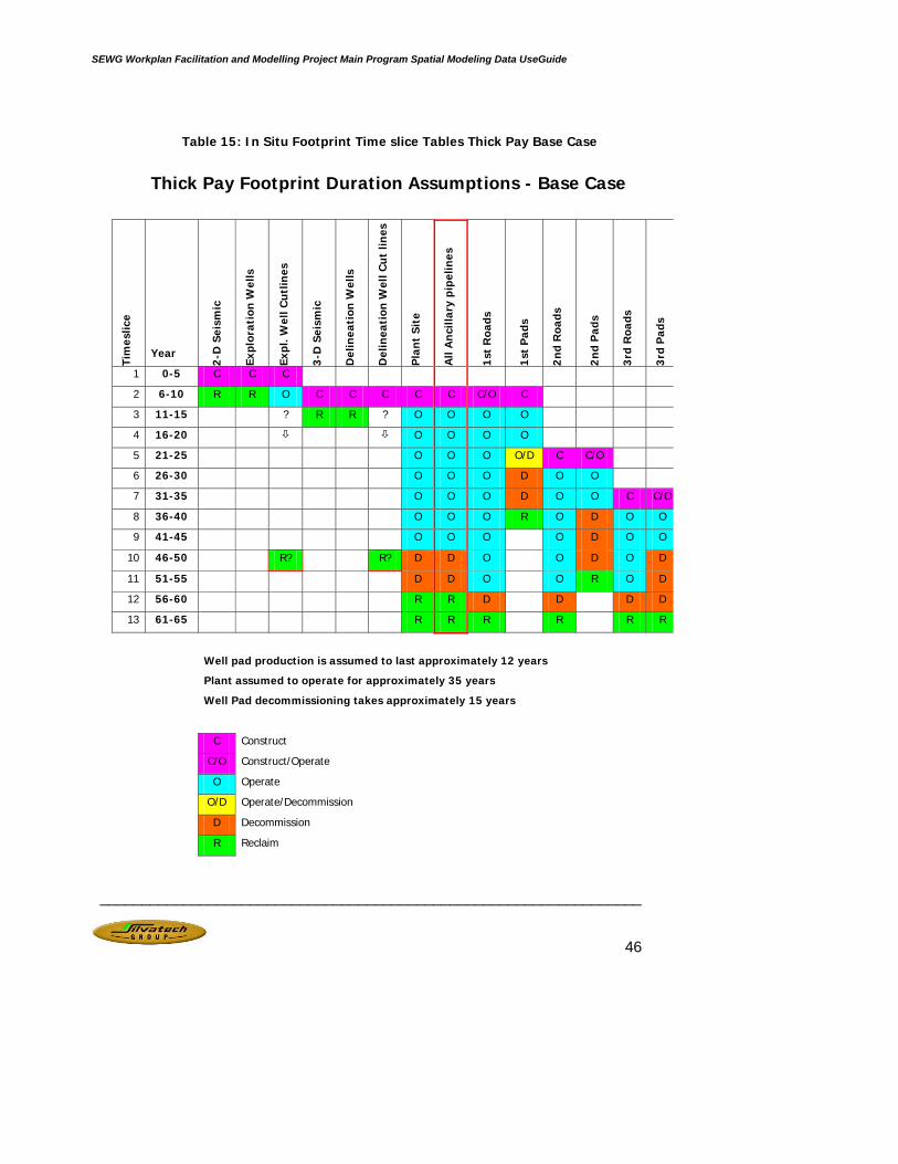
Table 15: In Situ Footprint Time slice Tables Thick Pay Base Case
Thick Pay Footprint Duration Assumptions - Base Case
Tim
eslic
e
Year
2-D
Sei
smic
Expl
orat
ion
Wel
ls
Expl
. Wel
l Cu
tlin
es
3-D
Sei
smic
Del
inea
tion
Wel
ls
Del
inea
tion
Wel
l Cu
t lin
es
Pla
nt
Sit
e
All
An
cilla
ry p
ipel
ines
1st
Roa
ds
1st
Pad
s
2n
d R
oads
2n
d P
ads
3rd
Roa
ds
3rd
Pad
s
1 0-5 C C C
2 6-10 R R O C C C C C C/O C
3 11-15 ? R R ? O O O O
4 16-20 O O O O
5 21-25 O O O O/D C C/O
6 26-30 O O O D O O
7 31-35 O O O D O O C C/O
8 36-40 O O O R O D O O
9 41-45 O O O O D O O
10 46-50 R? R? D D O O D O D
11 51-55 D D O O R O D
12 56-60 R R D D D D
13 61-65 R R R R R R
Well pad production is assumed to last approximately 12 years
Plant assumed to operate for approximately 35 years
Well Pad decommissioning takes approximately 15 years
C Construct
C/O Construct/Operate
O Operate
O/D Operate/Decommission
D Decommission
R Reclaim

SEWG Workplan Facilitation and Modelling Project Main Program Spatial Modeling Data UseGuide
_________________________________________________________________
47
Table 16: In Situ Footprint Time slice Tables Thick Pay Innovative Approaches
Thick Pay Footprint Duration Assumptions - Best Practice
Tim
eslic
e
Year
2-D
Sei
smic
Expl
orat
ion
Wel
ls
Expl
. Wel
l Cu
tlin
es
3-D
Sei
smic
Del
inea
tion
Wel
ls
Del
inea
tion
Wel
l Cu
t lin
es
Pla
nt
Sit
e
An
cilla
ry P
ipel
ines
1st
Roa
ds
1st
Pad
s
2n
d R
oads
2n
d P
ads
3rd
Roa
ds
3rd
Pad
s
1 0-5 C C C
2 6-10 R R O C C C C C C/O C
3 11-15 ? R R ? O O O O
4 16-20 O O O O
5 21-25 ? ? O O O O/D C C/O
6 26-30 R? R? O O O R O O
7 31-35 O O O O O C C/O
8 36-40 O O O O D O O
9 41-45 O O O O R O O
10 46-50 D D D D D D
11 51-55 D D R R R R
12 56-60 R R
Well pad production is assumed to last approximately 12 years
Plant assumed to operate for approximately 35 years
Well Pad decommissioning takes approximately 5 years
C Construct
C/O Construct/Operate
O Operate
O/D Operate/Decommission
D Decommission
R Reclaim
SEWG Workplan Facilitation and Modelling Project Main Program Spatial Modeling Data UseGuide
_________________________________________________________________
48
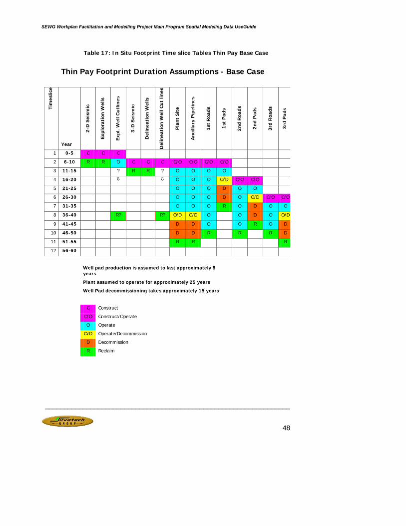
Table 17: In Situ Footprint Time slice Tables Thin Pay Base Case
Thin Pay Footprint Duration Assumptions - Base Case
Tim
eslic
e
Year
2-D
Sei
smic
Expl
orat
ion
Wel
ls
Expl
. Wel
l Cu
tlin
es
3-D
Sei
smic
Del
inea
tion
Wel
ls
Del
inea
tion
Wel
l Cu
t lin
es
Pla
nt
Sit
e
Anc
illar
y P
ipel
ines
1st
Roa
ds
1st
Pad
s
2nd
Roa
ds
2nd
Pad
s
3rd
Roa
ds
3rd
Pad
s
1 0-5 C C C
2 6-10 R R O C C C C/O C/O C/O C/O
3 11-15 ? R R ? O O O O
4 16-20 O O O O/D C/O C/O
5 21-25 O O O D O O
6 26-30 O O O D O O/D C/O C/O
7 31-35 O O O R O D O O
8 36-40 R? R? O/D O/D O O D O O/D
9 41-45 D D O O R O D
10 46-50 D D R R R D
11 51-55 R R R
12 56-60
Well pad production is assumed to last approximately 8 years
Plant assumed to operate for approximately 25 years
Well Pad decommissioning takes approximately 15 years
C Construct
C/O Construct/Operate
O Operate
O/D Operate/Decommission
D Decommission
R Reclaim
SEWG Workplan Facilitation and Modelling Project Main Program Spatial Modeling Data UseGuide
_________________________________________________________________
49
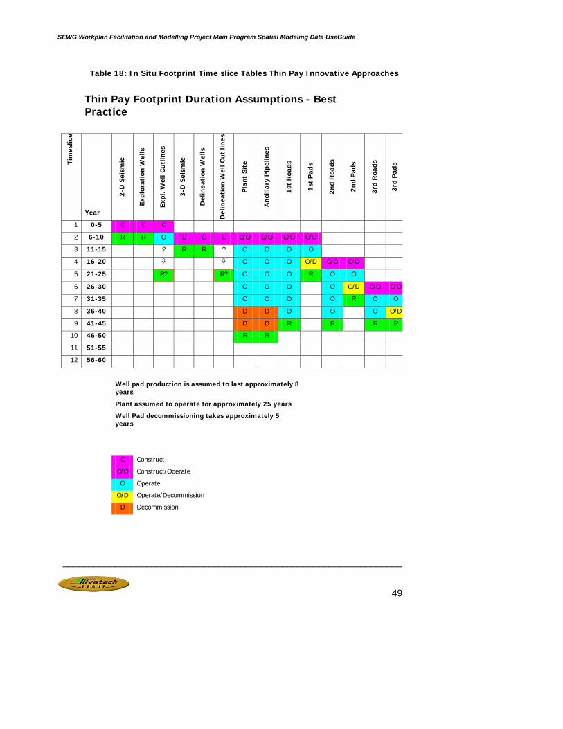
Table 18: In Situ Footprint Time slice Tables Thin Pay Innovative Approaches
Thin Pay Footprint Duration Assumptions - Best Practice
Tim
eslic
e
Year
2-D
Sei
smic
Expl
orat
ion
Wel
ls
Expl
. Wel
l Cut
lines
3-D
Sei
smic
Del
inea
tion
Wel
ls
Del
inea
tion
Wel
l Cu
t lin
es
Pla
nt
Sit
e
An
cilla
ry P
ipel
ines
1st
Roa
ds
1st
Pad
s
2nd
Roa
ds
2n
d P
ads
3rd
Roa
ds
3rd
Pad
s
1 0-5 C C C
2 6-10 R R O C C C C/O C/O C/O C/O
3 11-15 ? R R ? O O O O
4 16-20 O O O O/D C/O C/O
5 21-25 R? R? O O O R O O
6 26-30 O O O O O/D C/O C/O
7 31-35 O O O O R O O
8 36-40 D D O O O O/D
9 41-45 D D R R R R
10 46-50 R R
11 51-55
12 56-60
Well pad production is assumed to last approximately 8 years
Plant assumed to operate for approximately 25 years
Well Pad decommissioning takes approximately 5 years
C Construct
C/O Construct/Operate
O Operate
O/D Operate/Decommission
D Decommission
SEWG Workplan Facilitation and Modelling Project Main Program Spatial Modeling Data UseGuide
_________________________________________________________________
50
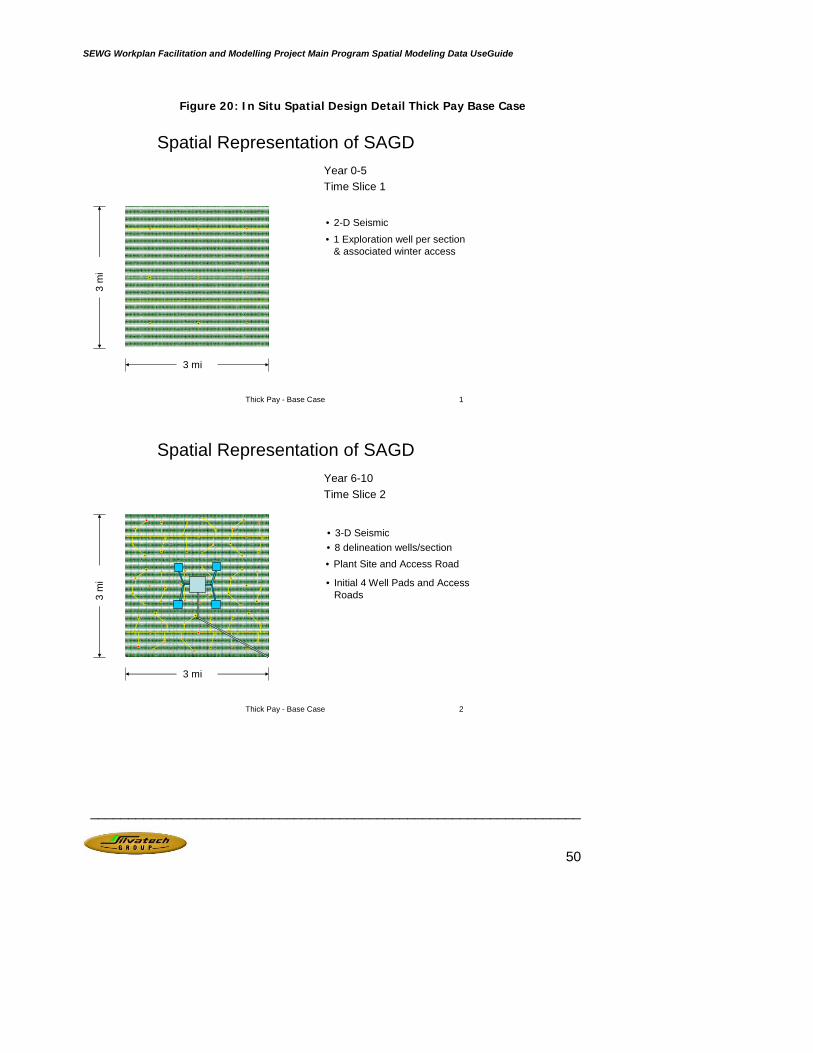
Figure 20: In Situ Spatial Design Detail Thick Pay Base Case
Thick Pay - Base Case 1
Spatial Representation of SAGDYear 0-5Time Slice 1
3 mi
3 m
i
• 2-D Seismic
• 1 Exploration well per section & associated winter access
Thick Pay - Base Case 2
• 3-D Seismic
Spatial Representation of SAGDYear 6-10Time Slice 2
3 mi
3 m
i
• 8 delineation wells/section• Plant Site and Access Road
• Initial 4 Well Pads and Access Roads
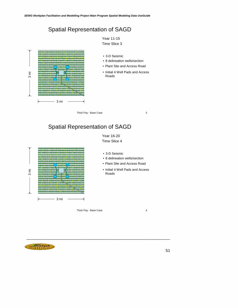
SEWG Workplan Facilitation and Modelling Project Main Program Spatial Modeling Data UseGuide
_________________________________________________________________
51
Thick Pay - Base Case 3
• 3-D Seismic
Spatial Representation of SAGDYear 11-15Time Slice 3
3 mi
3 m
i
• 8 delineation wells/section• Plant Site and Access Road
• Initial 4 Well Pads and Access Roads
Thick Pay - Base Case 4
• 3-D Seismic
Spatial Representation of SAGDYear 16-20Time Slice 4
3 mi
3 m
i
• 8 delineation wells/section• Plant Site and Access Road
• Initial 4 Well Pads and Access Roads
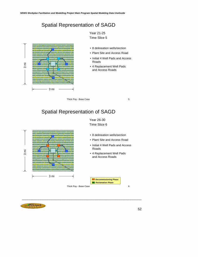
SEWG Workplan Facilitation and Modelling Project Main Program Spatial Modeling Data UseGuide
_________________________________________________________________
52
Thick Pay - Base Case 5
Spatial Representation of SAGDYear 21-25Time Slice 5
3 mi
3 m
i
• 8 delineation wells/section• Plant Site and Access Road
• Initial 4 Well Pads and Access Roads
• 4 Replacement Well Pads and Access Roads
Thick Pay - Base Case 6
Spatial Representation of SAGDYear 26-30Time Slice 6
3 mi
3 m
i
• 8 delineation wells/section
• Plant Site and Access Road
• Initial 4 Well Pads and Access Roads
• 4 Replacement Well Pads and Access Roads
Reclamation PhaseDecommissioning Phase
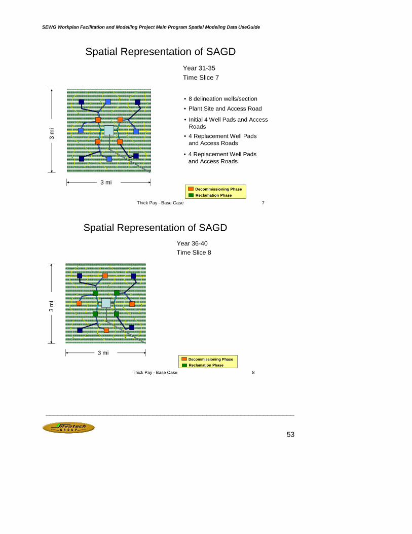
SEWG Workplan Facilitation and Modelling Project Main Program Spatial Modeling Data UseGuide
_________________________________________________________________
53
Thick Pay - Base Case 7
Spatial Representation of SAGDYear 31-35Time Slice 7
3 mi
3 m
i
• 8 delineation wells/section
• Plant Site and Access Road
• Initial 4 Well Pads and Access Roads
• 4 Replacement Well Pads and Access Roads
• 4 Replacement Well Pads and Access Roads
Reclamation PhaseDecommissioning Phase
Thick Pay - Base Case 8
Spatial Representation of SAGDYear 36-40Time Slice 8
3 mi
3 m
i
Reclamation PhaseDecommissioning Phase
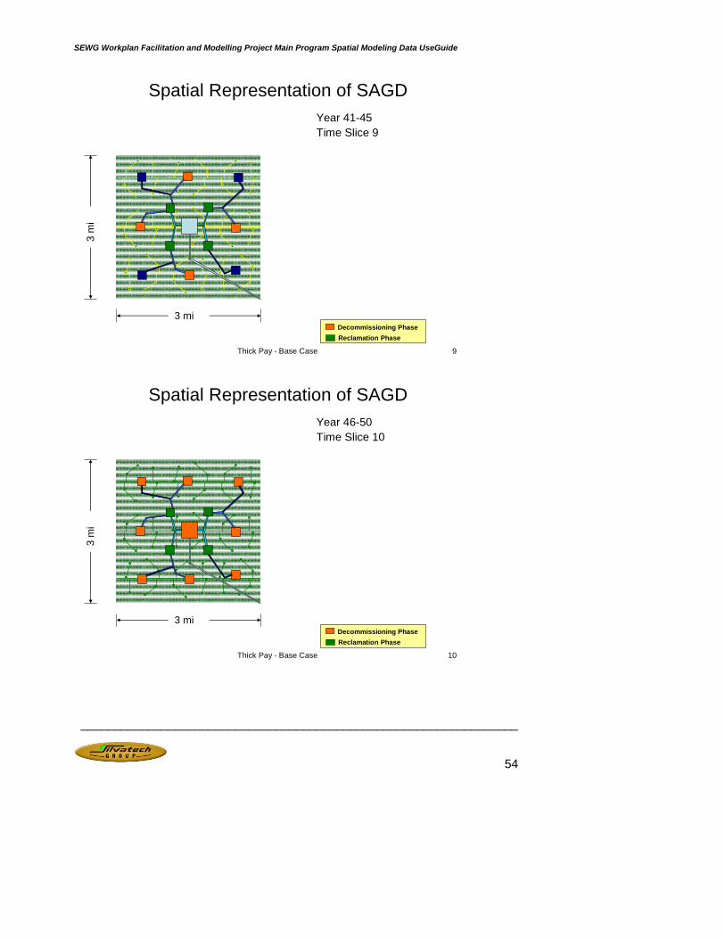
SEWG Workplan Facilitation and Modelling Project Main Program Spatial Modeling Data UseGuide
_________________________________________________________________
54
Thick Pay - Base Case 9
Spatial Representation of SAGDYear 41-45Time Slice 9
3 mi
3 m
i
Reclamation PhaseDecommissioning Phase
Thick Pay - Base Case 10
Spatial Representation of SAGDYear 46-50Time Slice 10
3 mi
3 m
i
Reclamation PhaseDecommissioning Phase
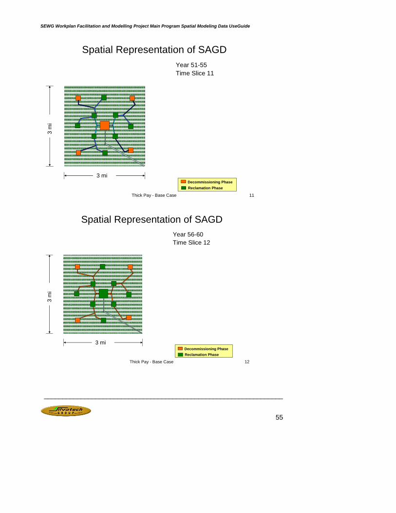
SEWG Workplan Facilitation and Modelling Project Main Program Spatial Modeling Data UseGuide
_________________________________________________________________
55
Thick Pay - Base Case 11
Spatial Representation of SAGDYear 51-55Time Slice 11
3 mi
3 m
i
Reclamation PhaseDecommissioning Phase
Thick Pay - Base Case 12
Spatial Representation of SAGDYear 56-60Time Slice 12
3 mi
3 m
i
Reclamation PhaseDecommissioning Phase

SEWG Workplan Facilitation and Modelling Project Main Program Spatial Modeling Data UseGuide
_________________________________________________________________
56
Thick Pay - Base Case 13
Spatial Representation of SAGDYear 61-65Time Slice 13
3 mi
3 m
i
Reclamation PhaseDecommissioning Phase
Thick Pay - Base Case 15
Spatial Representation of SAGD
3 mi
3 m
i
12 Well Pads
5 horizontal wellsDrainage area= 500 m X 800 m (40 ha)
12 pads X 2 drainage areas/pad = 24 drainage areas
2,331 ha
24 drainage areas X 40 ha = 960 ha
Drainage area coverage: 960 ha / 2,331 ha = 41%
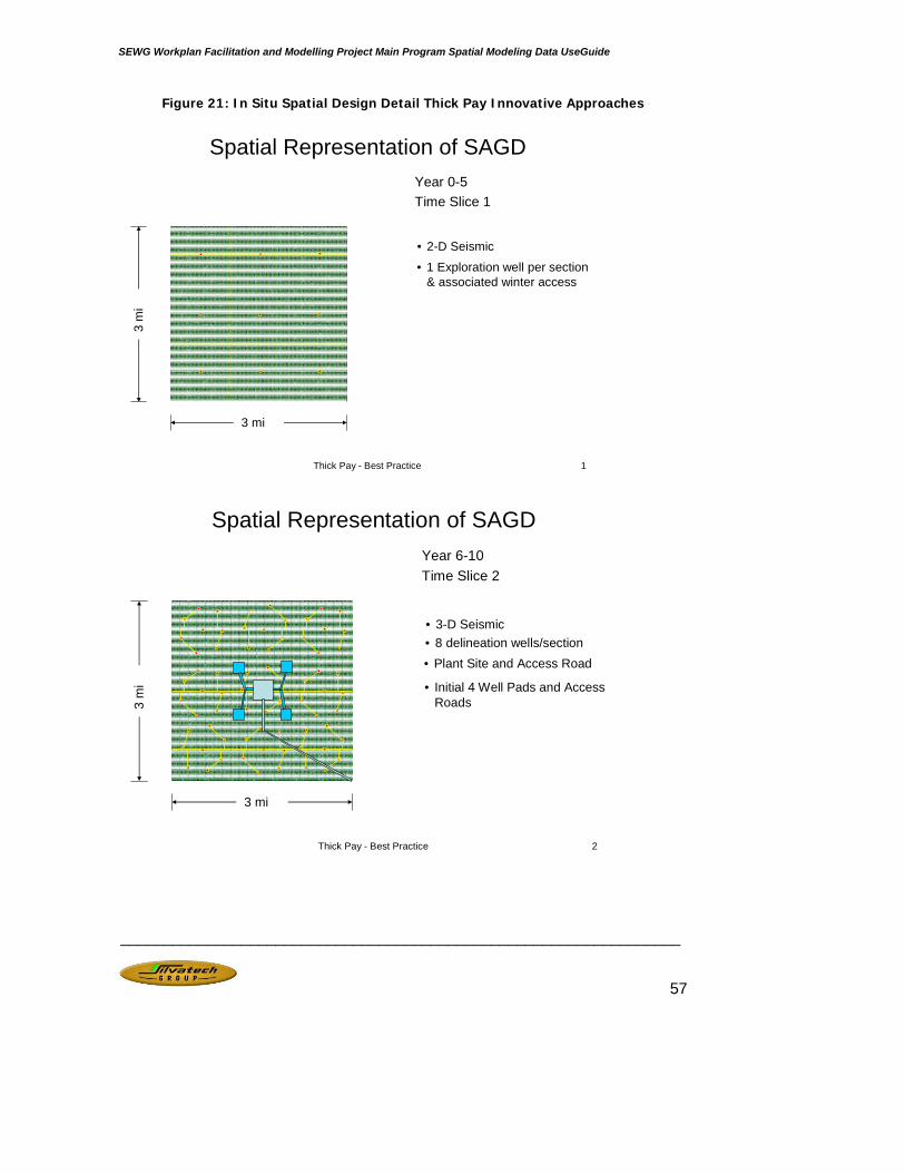
SEWG Workplan Facilitation and Modelling Project Main Program Spatial Modeling Data UseGuide
_________________________________________________________________
57
Figure 21: In Situ Spatial Design Detail Thick Pay Innovative Approaches
Thick Pay - Best Practice 1
Spatial Representation of SAGDYear 0-5Time Slice 1
3 mi
3 m
i
• 2-D Seismic
• 1 Exploration well per section & associated winter access
Thick Pay - Best Practice 2
• 3-D Seismic
Spatial Representation of SAGDYear 6-10Time Slice 2
3 mi
3 m
i
• 8 delineation wells/section• Plant Site and Access Road
• Initial 4 Well Pads and Access Roads
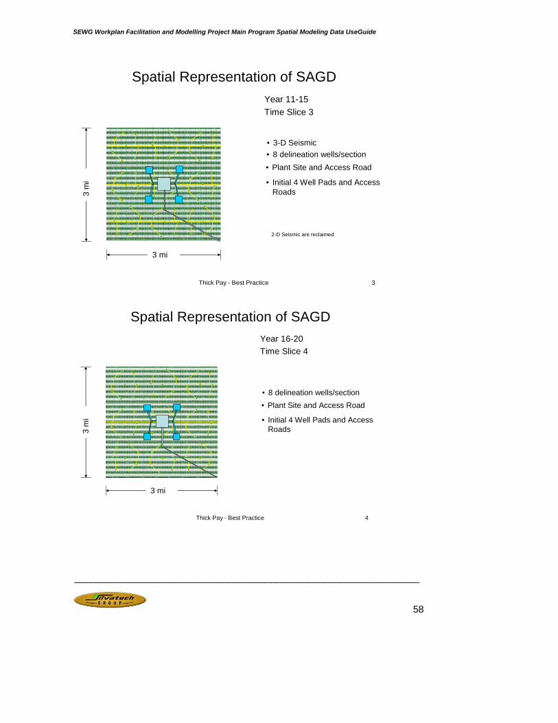
SEWG Workplan Facilitation and Modelling Project Main Program Spatial Modeling Data UseGuide
_________________________________________________________________
58
Thick Pay - Best Practice 3
• 3-D Seismic
Spatial Representation of SAGDYear 11-15Time Slice 3
3 mi
3 m
i
• 8 delineation wells/section• Plant Site and Access Road
• Initial 4 Well Pads and Access Roads
2-D Seismic are reclaimed
Thick Pay - Best Practice 4
Spatial Representation of SAGDYear 16-20Time Slice 4
3 mi
3 m
i
• 8 delineation wells/section• Plant Site and Access Road
• Initial 4 Well Pads and Access Roads
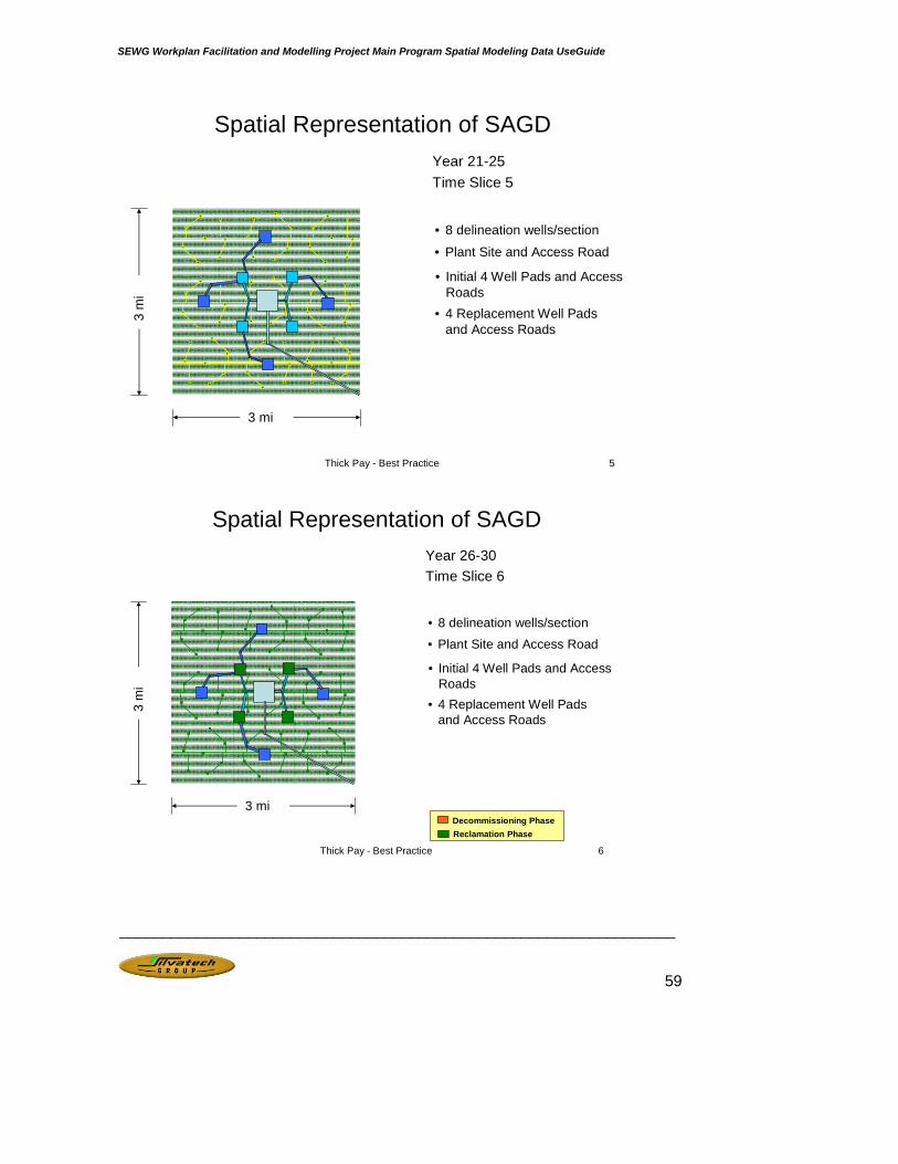
SEWG Workplan Facilitation and Modelling Project Main Program Spatial Modeling Data UseGuide
_________________________________________________________________
59
Thick Pay - Best Practice 5
Spatial Representation of SAGDYear 21-25Time Slice 5
3 mi
3 m
i
• 8 delineation wells/section
• Plant Site and Access Road
• Initial 4 Well Pads and Access Roads
• 4 Replacement Well Pads and Access Roads
Thick Pay - Best Practice 6
Spatial Representation of SAGDYear 26-30Time Slice 6
3 mi
3 m
i
• 8 delineation wells/section• Plant Site and Access Road
• Initial 4 Well Pads and Access Roads
• 4 Replacement Well Pads and Access Roads
Reclamation PhaseDecommissioning Phase

SEWG Workplan Facilitation and Modelling Project Main Program Spatial Modeling Data UseGuide
_________________________________________________________________
60
Thick Pay - Best Practice 7
Spatial Representation of SAGDYear 31-35Time Slice 7
3 mi
3 m
i
• Plant Site and Access Road
• Initial 4 Well Pads and Access Roads
• 4 Replacement Well Pads and Access Roads
• 4 Replacement Well Pads and Access Roads
Reclamation PhaseDecommissioning Phase
Thick Pay - Best Practice 8
Spatial Representation of SAGDYear 36-40Time Slice 8
3 mi
3 m
i
Reclamation PhaseDecommissioning Phase
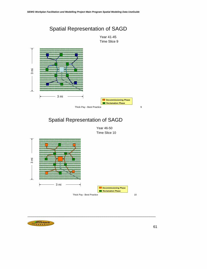
SEWG Workplan Facilitation and Modelling Project Main Program Spatial Modeling Data UseGuide
_________________________________________________________________
61
Thick Pay - Best Practice 9
Spatial Representation of SAGDYear 41-45Time Slice 9
3 mi
3 m
i
Reclamation PhaseDecommissioning Phase
Thick Pay - Best Practice 10
Spatial Representation of SAGDYear 46-50Time Slice 10
3 mi
3 m
i
Reclamation PhaseDecommissioning Phase
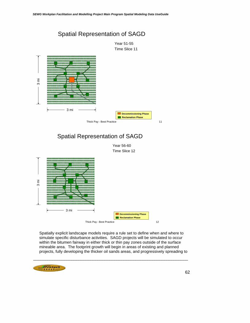
SEWG Workplan Facilitation and Modelling Project Main Program Spatial Modeling Data UseGuide
_________________________________________________________________
62
Thick Pay - Best Practice 11
Spatial Representation of SAGDYear 51-55Time Slice 11
3 mi
3 m
i
Reclamation PhaseDecommissioning Phase
Thick Pay - Best Practice 12
Spatial Representation of SAGDYear 56-60Time Slice 12
3 mi
3 m
i
Reclamation PhaseDecommissioning Phase
Spatially explicit landscape models require a rule set to define when and where to simulate specific disturbance activities. SAGD projects will be simulated to occur within the bitumen fairway in either thick or thin pay zones outside of the surface mineable area. The footprint growth will begin in areas of existing and planned projects, fully developing the thicker oil sands areas, and progressively spreading to
SEWG Workplan Facilitation and Modelling Project Main Program Spatial Modeling Data UseGuide
_________________________________________________________________
63
thinner zones as defined by the bitumen pay coverage over time at a rate consistent with projected production. Development will be allowed to occur except where more than 50% of the ¼ township grid overlies an urban area or a double line water feature. SAGD operations are assumed not to be permitted in these areas.
7.5. Forestry Because of the predominance of the projected energy sector development in this region, significant volumes of timber will be harvested to make way for oil extraction development. Because of existing policies that will charge harvested merchantable timber from energy sector development to forest tenure holders AAC, timber salvage activities associated with this development is expected to be a significant driver for forest sector activity. Therefore, timber salvaged from surface mineable and SAGD operations will be accounted for first during each simulation period. If, after all salvage activities for the period there remains a deficit of timber relative to the target AAC, harvesting will be simulated to take place first according to the spatial harvest sequence identified by Alpac in there DFMP and secondly from the remaining area designated for timber production according to the “oldest first” harvest queue rule.
7.5.1. Calculation of Allowable Annual Cut Because an Allowable Annual Cut (AAC) has not been determined for the RMWB, a target AAC volume will be calculated for the purposes of this project. A long-term non-declining harvest level will be computed using the following coarse procedure. The resulting AAC will be used to simulate timber harvest levels for both the ALCES and spatial models.
Step 1. Calculate the Net Productive Land base for the RMWB
From the gross land base, the following areas will be netted out to determine a commercially viable net productive land base:
Non-tenured lands: all forested lands that are not currently allocated for forest harvesting. In discussions with Alpac it was deemed that non FMA lands will be excluded from the productive land base for the purposes of this analysis. While it is recognized that there is some interest in timbered areas outside the FMA boundary (A9,A10, A11, A12, A13) there are no known tenures allocated or imminently planned and therefore these areas will not be included. These areas are shown on the map below:
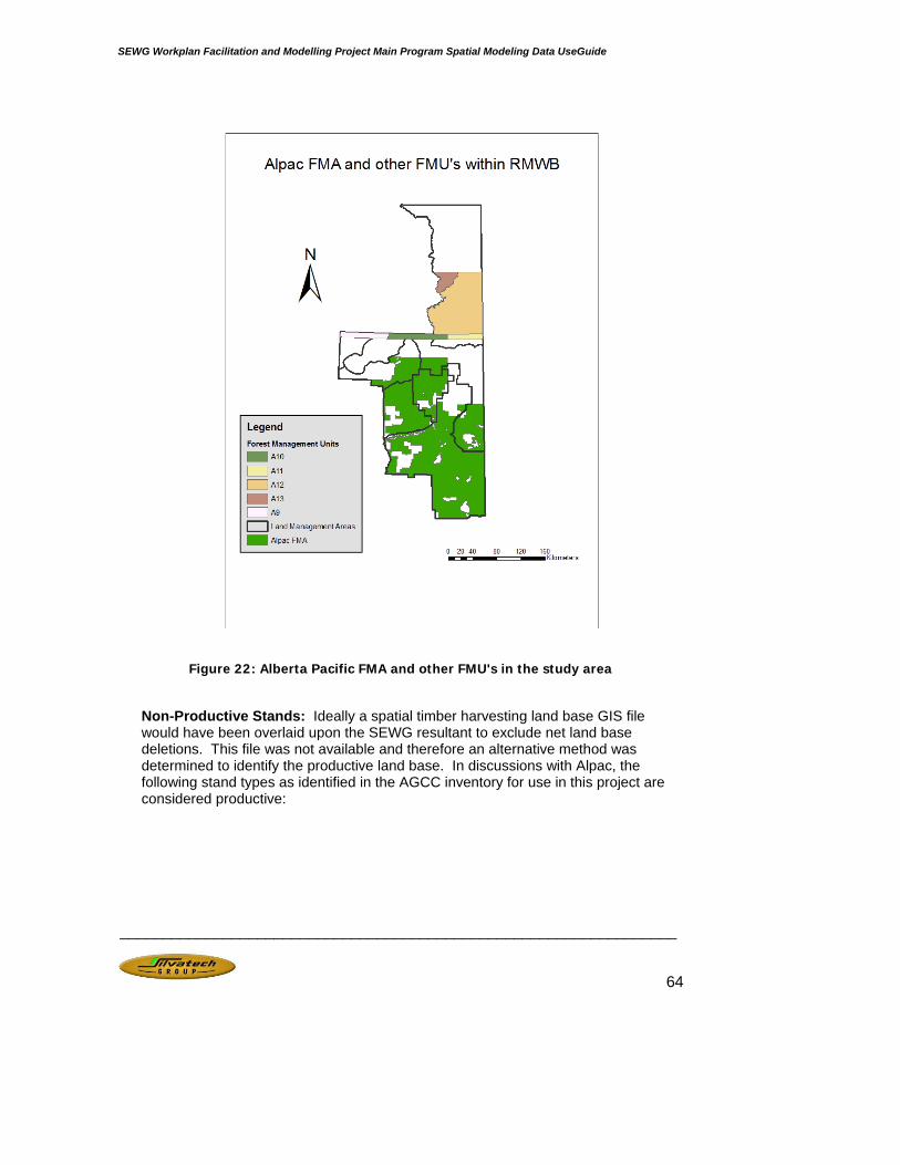
SEWG Workplan Facilitation and Modelling Project Main Program Spatial Modeling Data UseGuide
_________________________________________________________________
64
Figure 22: Alberta Pacific FMA and other FMU's in the study area
Non-Productive Stands: Ideally a spatial timber harvesting land base GIS file would have been overlaid upon the SEWG resultant to exclude net land base deletions. This file was not available and therefore an alternative method was determined to identify the productive land base. In discussions with Alpac, the following stand types as identified in the AGCC inventory for use in this project are considered productive:

SEWG Workplan Facilitation and Modelling Project Main Program Spatial Modeling Data UseGuide
_________________________________________________________________
65
Landscape Type AGCC Lable (AVI / AGCC) Description
52 Closed Pine5452 Closed Pine Leads Conifer
Hardwood 55 Closed aspen, balsam poplar and/or birtch56 Closed Coniferous Dominated
5650 Closed Fb dominated Mixedwood5652 Closed Pine dominated Mixedwood5653 Closed Sw dominated Mixedwood57 Closed Deciduous Dominated58 Closed Coniferous and Decidious Mixed153 Open White Spruce
154153 Open Sw Leads Conifer53 Closed White Spruce54 Closed undiffereniated coniferous
5450 Closed Fb Leads Conifer5453 Closed Sw Leads Conifer
Pine
Mixedwood
White Spruce
Table 19: Productive Forest Landscape Types
All black spruce stands and all open stands with the exception of open white spruce stands are excluded. While it is Alberta Pacific’s experience that approximately ½ of all jack pine leading stands are excluded, the inventory is not considered detailed enough to explicitly identify which stands in this group are in and which are out. Exclusion of these stands is assumed to be accounted for in determining the AAC using further aspatial netdown assumptions documented below but for the spatial delineation of the productive land base, all jack pine leading stands as identified in the above table will remain in the net productive land base. This is not assumed to introduce significant uncertainty to the scheduling of harvesting areas as a spatial harvest sequence provided by Alpac that already excludes these inoperable areas will be used to schedule non-salvage harvest.
Inoperable or unstable steep slopes: based on the Alpac DFMP, an aspatial reduction of 4.5% removal will be applied for the purposes of AAC determination. The spatial identification and removal of these sites will not be undertaken. This is not assumed to introduce significant uncertainty to the scheduling of harvesting areas as a spatial harvest sequence provided by Alpac that already excludes these inoperable areas will be used to schedule non-salvage harvest.
Greenup delay: based on the Alpac DFMP, an aspatial reduction of 10% removal will be applied for the purposes of AAC determination to account for stands ineligible for harvest due to greenup delay constraints.
Riparian buffers: based on the Alpac DFMP, an aspatial reduction of 2.2% removal will be applied for the purposes of AAC determination to account for stands ineligible for harvest because they are located within riparian buffers. During modelling, these riparian buffers have been explicitly identified and accounted for and harvest activity within them will not be permitted.
Inaccessible stands buffers: based on the Alpac DFMP, an aspatial reduction of 3% removal will be applied for the purposes of AAC determination to account for stands ineligible for harvest because they are considered inaccessible or isolated. The spatial identification and removal of these sites will not be undertaken. This is

SEWG Workplan Facilitation and Modelling Project Main Program Spatial Modeling Data UseGuide
_________________________________________________________________
66
not assumed to introduce significant uncertainty to the scheduling of harvesting areas as a spatial harvest sequence provided by Alpac that already excludes these inoperable areas will be used to schedule non-salvage harvest. Protected Areas: for the protected areas scenario, the proposed Canadian Parks and Wilderness Protected Areas Network will be removed from the net productive land base and stands growing in this area will not contribute to the AAC. Existing protected areas area also excluded for all scenarios.
Step 2. Calculate Annual Harvest volumes for both hardwood and softwood. Once the Net Productive Land base has been determined (Step 1 above), the Mean Annual Increment (MAI) values currently used for the Alpac FMA will be applied to compute an annual harvest volume.
Step 3. The harvest volumes computed in Step 2 will be applied to the land base and the merchantable stands will be grown based on the Average Site Growth and Yield curves provided by Alpac as derived for use in their DFMP. Harvest levels will be simulated on the RMWB for a minimum of 2 rotations (200 years) to ensure that they generate a non-declining (sustainable) cut level. If a non-declining harvest trajectory can not be achieved harvest targets will be lowered until sustainability can be demonstrated by the achievement of stable long term growing stock. Once the non-declining harvest level has been determined it will serve as the harvest target for both the ALCES and spatial modelling.
8. Projection Time Horizon The Main Program Modelling will project disturbances and monitor indicator performance over a 100-year time horizon. Time 0 is assumed to be 2006. ALCES modelling will be projected on an annual basis. In order to reduce data processing requirements, the spatially explicit modelling will be simulated in 5-year periods.
SEWG Workplan Facilitation and Modelling Project Main Program Spatial Modeling Data UseGuide
_________________________________________________________________
67
9. SCENARIOS FOR MAIN PROGRAM MODELLING
9.1. Base Case (Control) Scenarios
9.1.1. Guiding Principles: • Is a snapshot in time representative of current policies, practices and
technologies.
• Is a benchmark against which the other scenarios can be compared to evaluate alternative management outcomes.
• Assumes that present practices will continue for the duration of the forecast.
• Uses the best available Traditional Environmental Knowledge, scientific data and information as provided by SEWG to Silvatech.
9.1.2. Narrative: The Base Case scenario represents the way things are done today and assumes that current practices, policies, market forces etc. remain unchanged. The Base Case is a benchmark against which indicator performance in all other management option scenarios can be compared and evaluated.
9.2. Protected Areas Scenario
9.2.1. Guiding Principles: • Accepts the basic premise that the recommended Protected Areas will
adequately maintain ecosystem integrity.
• Is based on the work of Al-Pac, CPAWS and the Pembina Institute.
• Minimize conflict with the energy sector where possible
9.2.2. Narrative: The ecosystem best practices scenario explores the concept that the purposeful preservation of specific areas in their natural state is an effective way to ensure adequate protection of ecosystems to help maintain long-term sustainability in the RMWB. In this scenario, the first management priority is to maintain natural ecosystem integrity.
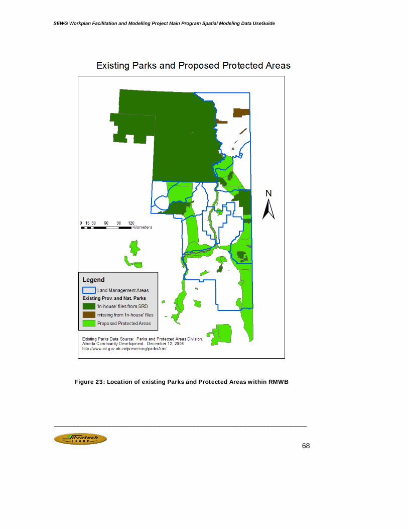
SEWG Workplan Facilitation and Modelling Project Main Program Spatial Modeling Data UseGuide
_________________________________________________________________
68
Figure 23: Location of existing Parks and Protected Areas within RMWB

SEWG Workplan Facilitation and Modelling Project Main Program Spatial Modeling Data UseGuide
_________________________________________________________________
69
9.3. Innovative Approaches Scenario
9.3.1. Guiding Principles: • New and innovative approaches.
• Future footprint/bitumen disturbance ratios decrease with technological advances
• Cross industry joint planning to minimizing cumulative footprint spatially and temporally
• Employs a concept of BATEA (Best Available Technology Economically Achievable) and is assumed not to increase capital accrual costs and or royalty reductions not to exceed 10%
• Human access management
9.3.2. Narrative: The evolving approaches scenario will provide SEWG with the opportunity to consider how new and innovative practices could be applied to reduce the overall human footprint and its associated impacts. The scenario is intended to capture the maximum opportunity for multi-user cooperative planning and the full benefit of scientific and operations advancement.
9.4. Access Management Scenario
9.4.1. Guiding Principles: • Minimize the construction of linear features
• Limit human utility of linear features for movement
• Influence predator utility of linear features for movement and hunting
9.4.2. Narrative: The access management scenario will provide SEWG with the opportunity to consider how practices aimed at minimizing the construction of linear features as well as those aimed at minimizing the effective utility of features that are constructed for movement by both humans and predators.

SEWG Workplan Facilitation and Modelling Project Main Program Spatial Modeling Data UseGuide
_________________________________________________________________
70
Table 20: Access Management Assumptions Summary