Generalized Minimum Bias Models By Luyang Fu, Ph. D. Cheng-sheng Peter Wu, FCAS, ASA, MAAA.
Upload
sarah-kelleyCategory
view
221download
0
Severity Distributions for GLMs: Gamma or Lognormal?
Presented by
Luyang Fu, Grange Mutual
Richard Moncher, Bristol West
2004 CAS Spring Meeting
Colorado Springs, Colorado
May 18, 2004

2
Session Outline
Introduction
Distribution Assumptions
Simulation Method
Simulation Results
Conclusions

3
Introduction
Common characteristics of loss distributions
Typical GLM forms in actuarial practice
Lognormal and Gamma are most widely-used distributions in size of loss (severity) analysis
Lognormal or Gamma?

4
Distribution Characteristics of Insurance Losses
Non-negative
Positively skewed
Variance is positively correlated with mean.
Normal is not appropriate:
negative,
symmetric,
constant variance

5
Advantages of GLMsExponential Distribution Selections:
Poisson, Gamma, Binomial, Inverse Gaussian, Negative Binomial, etc.
Lognormal is not in exponential family.
Link Function Selections:
Identity, Log, Logit, Power, Probit, etc.

6
Typical GLM Forms in Actuarial Practice
Severity:
Log link, Gamma Distribution
Frequency:
Log link, Poisson Distribution
Retention (Renewal):
Logit link, Binomial Distribution

7
Gamma or Lognormal?
Gamma and lognormal are the two most popular selections of loss distributions
On CAS website (www.casact.org), we found 31 papers by searching “Lognormal” and 37 papers by searching “Gamma”

8
Lognormal Is One of Most Widely-Used Loss Distributions
Proceedings of the Casualty Actuarial Society
Ratemaking and ReinsuranceWacek, Michael G.(1997)Bear, Robert A.; Nemlick, Kenneth J. (1990)Hayne, Roger M. (1985)Mack, Thomas (1984)Ter Berg, Peter (1980)Benckert, Lars-Gunnar (1962)

9
Lognormal Is One of Most Widely-Used Loss Distributions
Proceedings of the Casualty Actuarial Society
Reserving and Reinsurance
Kreps, Rodney E. (1997)
Ramsay, Colin M.; Usabel, Miguel A. (1997)
Doray, Louis G. (1996)
Levi, Charles; Partratm, Christian (1991)
Hertig, Joakim (1985)

10
Lognormal Is One of Most Widely-Used Loss Distributions
In actuarial practice
Increased Limit Factors
Excess of Loss Calculations
Weather Load Quantile
Loss Reserve Variability

11
Gamma or Lognormal?
Desirable Features of Gamma and Lognormal Distributions:
1. Non-negative
2. Positively skewed
3. Variance is proportional to the mean-squared (Constant Coefficient of Variation)

12
Gamma or Lognormal?Advantages of Lognormal:
Easy to understand (related to normal distribution)Consistent with other actuarial procedures, such as increased limits ratemakingFits data with large skewness well
Disadvantage of Lognormal:Not in exponential family, and GLM coefficients need volatility adjustment

13
Gamma or Lognormal?
Under what conditions are the severity distribution assumptions important?
If severity distribution is unknown, which distribution yields most accurate and stable results (i.e., minimized estimation bias and standard error)?

14
Classical Distribution Assumptions
Normal
Constant Variance
Gamma
Constant Coefficient of Variation
),( 2iN
2 VarianceMean i
2ii VarianceMean
),( iG
2
1

15
Classical Distribution Assumptions
Lognormal
Constant Coefficient of Variation
),( iML
2/2 iMeMean
)1(222 eeVariance iM
)1(2
e

16
Does Normal Necessarily Imply Constant Variance?
NormalConstant Coefficient of Variation:
Variance function is like Gamma
NormalVariance proportional to mean:
Variance function is like Poisson
),( 22 iiN
),( 2 iiN
MeanVarSqrt /)(
2σMeanVar /

17
Does Gamma Necessarily Imply Constant Coefficient of Variation?
Gamma
Variance is proportional to mean:
Variance function is like Poisson.
θ),G(αi
2 ii VarianceMean
θMean / Variance

18
Distribution Assumptions
One of two parameters is constantWhich one is selected as constant should be based on data Classical assumptions are most-widely used distribution forms, and generally fit data betterCan we assume none of them are constant?Yes, but it will increase the number of parameters and reduce the degrees of freedom

19
Why Simulation?
The distributions of GLM coefficients and predicted values are unknown in the case of small samples
Statistical analysis based on asymptotic distributions is not reliable
In an individual regression, we don’t know if the difference between predicted value and observed value is from random variation or systematic bias

20
Simulation Assumptions
32 Severity Observations for Two Class Variables
8 Age Groups
4 Vehicle-Use Groups
Data Source: Private Passenger Auto Collision used in Mildenhall (1999) and McCullagh and Nelder (1989)

21
Simulation Assumptions
Individual Losses Have Constant Coefficient of Variation
Multiplicative Relationship Between Severities and Rating Variables
Known “True” Base Severities & Relativities
Known CVs for the Severity Distribution

22
Simulation Procedures
1. Generate individual losses based on lognormal and gamma distributions and calculate 32 claim severities
2. Fit three regressions: GLM with Gamma, GLM with Normal, and GLM with log-transformed severity
3. Repeat Steps 1-2 one thousand times, and generate sampling distributions of GLM coefficients and predicted values

23
Performance Measurements
Weighted Absolute Bias, which measures the systematic bias (accuracy):
Weighted Standard Error, which measures random variation (stability):
ji
jijiji
w
SSEwwab
,
,,, |)ˆ(|
ji
jiji
w
wwse
,
,,

24
Adjustments for Log-Transformed Regressions
GLMs with Gamma and Normal
Log-transformed Regression
is called the “Volatility Adjustment Factor”
jijiji nbaji eeS ,
2, 2intercept
, *ˆ
ji baji eeS *ˆ intercept
,
jiji ne ,2, 2

25
Simulation Results
Data Generated
Regression Results
Residual Diagnostics

26
Data Generated
Reporting on Two Different Classes:
Classification I - Age 17-20 and Pleasure Use, with 21 observations.
Classification II - Age 40-49 and Short Drive to Work, with 970 observations.

27
Data Generated: Gamma Severity for Age 17-20 and Pleasure Use with Coefficient of Variation 3.0
simulations
Se
ve
rity
0 200 400 600 800 1000
02
00
40
06
00
80
0
simulated severity for age 17-20 for pleasure
severity
de
nsity
-200 0 200 400 600 800 1000 1200
0.0
0.0
01
00
.00
20
severity density for age 17-20 for pleasure
Quantiles of Standard Normal
Se
ve
rity
-2 0 2
02
00
40
06
00
80
0
severity QQ Plot for age 17-20 for pleasure
0 200 400 600 800 1000 1200
05
01
00
15
02
00
25
03
00
Severity
Sim
ula
tio
ns
severity histogram for age 17-20 for pleasure

28
Data Generated: Gamma Severity for Age 40-49 and DTW Short Use with Coefficient of Variation 3.0
simulations
Se
ve
rity
0 200 400 600 800 1000
16
01
80
20
02
20
24
02
60
simulated severity for age 40-49 for DTW Short
severity
de
nsity
140 160 180 200 220 240 260 280
0.0
0.0
05
0.0
10
0.0
15
severity density for age 40-49 for DTW Short
Quantiles of Standard Normal
Se
ve
rity
-2 0 2
16
01
80
20
02
20
24
02
60
severity QQ Plot for age 40-49 for DTW Short
160 180 200 220 240 260
05
01
00
15
02
00
Severity
Sim
ula
tio
ns
severity histogram for age 40-49 for DTW Short

29
Data Generated: Lognormal Severity for Age 17-20 and Pleasure Use with Coefficient of Variation 3.0
simulations
Se
ve
rity
0 200 400 600 800 1000
01
00
02
00
03
00
04
00
0
simulated severity for age 17-20 for pleasure
severity
de
nsity
0 1000 2000 3000 4000 5000
0.0
0.0
00
50
.00
15
severity density for age 17-20 for pleasure
Quantiles of Standard Normal
Se
ve
rity
-2 0 2
01
00
02
00
03
00
04
00
0
severity QQ Plot for age 17-20 for pleasure
0 500 1000 1500 2000
01
00
20
03
00
Severity
Sim
ula
tio
ns
severity histogram for age 17-20 for pleasure

30
Data Generated: Lognormal Severity for Age 40-49 and DTW Short Use with Coefficient of Variation 3.0
simulations
Se
ve
rity
0 200 400 600 800 1000
16
02
00
24
02
80
simulated severity for age 40-49 for DTW Short
severity
de
nsity
150 200 250 300
0.0
0.0
05
0.0
15
severity density for age 40-49 for DTW Short
Quantiles of Standard Normal
Se
ve
rity
-2 0 2
16
02
00
24
02
80
severity QQ Plot for age 40-49 for DTW Short
160 180 200 220 240 260 280
05
01
00
15
02
00
Severity
Sim
ula
tio
ns
severity histogram for age 40-49 for DTW Short

31
Regression ResultsOverall Unbiasedness and Stability
of Predicted Severities for Gamma Loss
CV wab wse
G-G G-L G-N G-G G-L G-N
1.0 0.180 0.240 0.221 8.170 8.177 8.568
2.0 0.475 0.852 0.509 16.498 16.514 17.239
3.0 0.860 1.808 1.139 25.223 25.097 26.986

32
Regression ResultsOverall Unbiasedness and Stability
of Predicted Severities for Lognormal Loss
CV wab wse
L-G L-L L-N L-G L-L L-N
1.0 0.151 0.202 0.175 8.309 8.284 8.754
2.0 0.498 0.844 0.604 16.426 16.113 17.721
3.0 0.720 1.589 1.006 24.328 23.214 27.608

33
Regression Results: Predicted Severities for Gamma Loss with Coefficient of Variation 3.0 for Age 17-20 and Pleasure Use
simulations
Pre
dic
ted
Se
ve
rity
0 200 400 600 800 1000
10
03
00
50
0
G-G severity for 17-20 and pleasure
severity
de
nsity
0 200 400 600
0.0
0.0
02
0.0
04
G-G severity density for 17-20 and pleasure
simulations
Pre
dic
ted
Se
ve
rity
0 200 400 600 800 1000
10
03
00
50
0
G-L severity for 17-20 and pleasure
severityd
en
sity
0 200 400 600
0.0
0.0
02
0.0
04
G-L severity density for 17-20 and pleasure
simulations
Pre
dic
ted
Se
ve
rity
0 200 400 600 800 1000
10
03
00
50
07
00
G-N severity for 17-20 and pleasure
severity
de
nsity
0 200 400 600
0.0
0.0
02
0.0
04
G-N severity density for 17-20 and pleasure

34
Regression Results: Predicted Severities for Gamma Loss with Coefficient of Variation 3.0 for Age 40-49 and DTW Short Use
simulations
Pre
dic
ted
Se
ve
rity
0 200 400 600 800 1000
16
02
00
24
0
G-G severity for 40-49 and DTW Short
severity
de
nsity
140 160 180 200 220 240 260 280
0.0
0.0
10
0.0
25
G-G severity density for 40-49 and DTW Short
simulations
Pre
dic
ted
Se
ve
rity
0 200 400 600 800 1000
16
02
00
24
0
G-L severity for 40-49 and DTW Short
severityd
en
sity
140 160 180 200 220 240 260 280
0.0
0.0
10
0.0
25
G-L severity density for 40-49 and DTW Short
simulations
Pre
dic
ted
Se
ve
rity
0 200 400 600 800 1000
16
02
00
24
0
G-N severity for 40-49 and DTW Short
severity
de
nsity
140 160 180 200 220 240 260
0.0
0.0
10
0.0
20
G-N severity density for 40-49 and DTW Short

35
Regression Results: Predicted Severities for Lognormal Loss with Coefficient of Variation 3.0 for Age 17-20 and Pleasure Use
simulations
Pre
dic
ted
Se
ve
rity
0 200 400 600 800 1000
20
06
00
10
00
L-G severity for 17-20 and pleasure
severity
de
nsity
0 200 400 600 800 1000 1200 1400
0.0
0.0
02
0.0
05
L-G severity density for 17-20 and pleasure
simulations
Pre
dic
ted
Se
ve
rity
0 200 400 600 800 1000
10
03
00
50
07
00
L-L severity for 17-20 and pleasure
severity
de
nsity
0 200 400 600 800
0.0
0.0
03
0.0
06
L-L severity density for 17-20 and pleasure
simulations
Pre
dic
ted
Se
ve
rity
0 200 400 600 800 1000
01
00
02
00
0
L-N severity for 17-20 and pleasure
severity
de
nsity
0 1000 2000 3000
0.0
0.0
01
5L-N severity density for 17-20 and pleasure
36
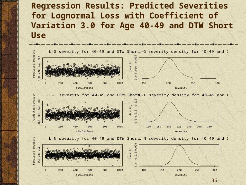
Regression Results: Predicted Severities for Lognormal Loss with Coefficient of Variation 3.0 for Age 40-49 and DTW Short Use
simulations
Pre
dic
ted
Se
ve
rity
0 200 400 600 800 1000
16
02
00
24
02
80
L-G severity for 40-49 and DTW Short
severity
de
nsity
150 200 250 300
0.0
0.0
10
0.0
25
L-G severity density for 40-49 and DTW Short
simulations
Pre
dic
ted
Se
ve
rity
0 200 400 600 800 1000
16
02
00
24
02
80
L-L severity for 40-49 and DTW Short
severityd
en
sity
160 180 200 220 240 260 280
0.0
0.0
10
0.0
25
L-L severity density for 40-49 and DTW Short
simulations
Pre
dic
ted
Se
ve
rity
0 200 400 600 800 1000
15
02
00
25
0
L-N severity for 40-49 and DTW Short
severity
de
nsity
100 150 200 250 300
0.0
0.0
10
0.0
20
L-N severity density for 40-49 and DTW Short

37
Residual Diagnostics: Standardized Residuals for Gamma Loss with Coefficient of Variation 3.0
Quantiles of Standard Normal
Pe
ars
on
Re
sid
ua
ls
-2 -1 0 1 2
-3-2
-10
1
G-G Pearson Residuals QQ Plot
Quantiles of Standard Normal
De
via
nce
Re
sid
ua
ls
-2 -1 0 1 2
-3-2
-10
1
G-G Deviance Residuals QQ Plot
Quantiles of Standard Normal
Re
sid
ua
ls
-2 -1 0 1 2
-3-2
-10
1
G-L Residuals QQ Plot
Quantiles of Standard Normal
Re
sid
ua
ls
-2 -1 0 1 2
-3-2
-10
12
G-N Residuals QQ Plot
38
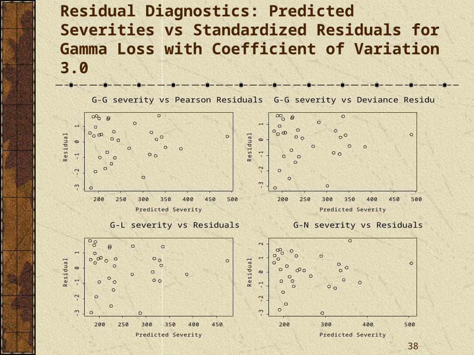
Residual Diagnostics: Predicted Severities vs Standardized Residuals for Gamma Loss with Coefficient of Variation 3.0
Predicted Severity
Re
sid
ua
l
200 250 300 350 400 450 500
-3-2
-10
1
G-G severity vs Pearson Residuals
Predicted Severity
Re
sid
ua
l
200 250 300 350 400 450 500
-3-2
-10
1
G-G severity vs Deviance Residuals
Predicted Severity
Re
sid
ua
l
200 250 300 350 400 450
-3-2
-10
1
G-L severity vs Residuals
Predicted Severity
Re
sid
ua
l
200 300 400 500
-3-2
-10
12
G-N severity vs Residuals

39
Residual Diagnostics: Standardized Residuals for Lognormal Loss with Coefficient of Variation 3.0
Quantiles of Standard Normal
Pe
ars
on
Re
sid
ua
ls
-2 -1 0 1 2
-2-1
01
23
L-G Pearson Residuals QQ Plot
Quantiles of Standard Normal
De
via
nce
Re
sid
ua
ls
-2 -1 0 1 2
-2-1
01
2
L-G Deviance Residuals QQ Plot
Quantiles of Standard Normal
Re
sid
ua
ls
-2 -1 0 1 2
-2-1
01
2
L-L Residuals QQ Plot
Quantiles of Standard Normal
Re
sid
ua
ls
-2 -1 0 1 2
-3-2
-10
12
3
L-N Residuals QQ Plot

40
Residual Diagnostics: Predicted Severities vs Standardized Residuals for Lognormal Loss with Coefficient of Variation 3.0
Predicted Severity
Re
sid
ua
l
200 300 400 500
-2-1
01
23
L-G severity vs Pearson Residuals
Predicted Severity
Re
sid
ua
l
200 300 400 500
-2-1
01
2
L-G severity vs Deviance Residuals
Predicted Severity
Re
sid
ua
l
200 300 400 500
-2-1
01
2
L-L severity vs Residuals
Predicted Severity
Re
sid
ua
l
200 300 400 500
-3-2
-10
12
3
L-N severity vs Residuals

41
Residual Diagnostics: Standardized Residuals for Gamma Loss with Coefficient of Variation 1.0 Based on Individual Data
Quantiles of Standard Normal
Pe
ars
on
Re
sid
ua
ls
-4 -2 0 2 4
02
46
81
01
2
G-G Pearson Residuals QQ Plot
Quantiles of Standard Normal
De
via
nce
Re
sid
ua
ls
-4 -2 0 2 4
-4-2
02
4
G-G Deviance Residuals QQ Plot
Quantiles of Standard Normal
Re
sid
ua
ls
-4 -2 0 2 4
-6-4
-20
2
G-L Residuals QQ Plot
Quantiles of Standard Normal
Re
sid
ua
ls
-4 -2 0 2 4
-20
24
68
10
G-N Residuals QQ Plot

42
Residual Diagnostics: Predicted Severities vs Standardized Residuals for Gamma Loss with Coefficient of Variation 1.0 Based on Individual Data
Predicted Severity
Re
sid
ua
l
200 300 400 500
02
46
81
01
2
G-G severity vs Pearson Residuals
Predicted Severity
Re
sid
ua
l
200 300 400 500
-4-2
02
4
G-G severity vs Deviance Residuals
Predicted Severity
Re
sid
ua
l
150 200 250 300 350 400
-6-4
-20
2
G-L severity vs Residuals
Predicted Severity
Re
sid
ua
l
200 300 400 500
-20
24
68
10
G-N severity vs Residuals
43
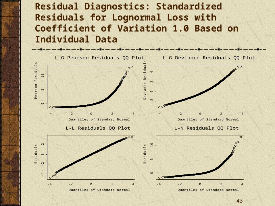
Residual Diagnostics: Standardized Residuals for Lognormal Loss with Coefficient of Variation 1.0 Based on Individual Data
Quantiles of Standard Normal
Pe
ars
on
Re
sid
ua
ls
-4 -2 0 2 4
05
10
L-G Pearson Residuals QQ Plot
Quantiles of Standard Normal
De
via
nce
Re
sid
ua
ls
-4 -2 0 2 4
-20
24
L-G Deviance Residuals QQ Plot
Quantiles of Standard Normal
Re
sid
ua
ls
-4 -2 0 2 4
-4-2
02
L-L Residuals QQ Plot
Quantiles of Standard Normal
Re
sid
ua
ls
-4 -2 0 2 4
05
10
L-N Residuals QQ Plot

44
Residual Diagnostics: Predicted Severities vs Standardized Residuals for Lognormal Loss with Coefficient of Variation 1.0 Based on Individual Data
Predicted Severity
Re
sid
ua
l
200 250 300 350 400
05
10
L-G severity vs Pearson Residuals
Predicted Severity
Re
sid
ua
l
200 250 300 350 400
-20
24
L-G severity vs Deviance Residuals
Predicted Severity
Re
sid
ua
l
200 250 300 350 400
-4-2
02
4
L-L severity vs Residuals
Predicted Severity
Re
sid
ua
l
200 250 300 350 400
05
10
L-N severity vs Residuals

45
Conclusions
When the gamma distribution is “true”, the G-G model is dominant in both unbiasedness and stability (except the G-L model is slightly more stable in the case of large volatility).

46
Conclusions
When the lognormal distribution is “true”, the L-L model is dominant in terms of stability.

47
ConclusionsGLMs with a normal distribution never dominate based on any criteria, and they have the worst weighted standard error.

48
Conclusions
GLMs with a gamma distribution are dominant in terms of unbiasedness, no matter whether the “true” distribution is gamma or lognormal.

49
Conclusions
In general, GLMs with a gamma distribution are recommended because they perform slightly better than the log-transformed model.

50
Conclusions
When the data is not volatile, the distribution selection for GLMs may not be as important because all distribution assumptions yield small biases and standard errors.
51
ConclusionsWhen the data is very volatile, the log-transformed regression is recommended because it provides the most stable estimation.

52
Conclusions
When the log-transformed model is used, the classification relativities should be adjusted by a volatility-adjustment factor. Without the adjustment, the relativities could be undervalued.

53
ConclusionsResidual plots may work well to examine the distribution assumptions on individual data, but not necessarily on summarized/average data.

54
Questions & Answers
Questions?
Thank You!