SET-WET: A WETLAND SIMULATION MODEL TO OPTIMIZE …

SET-WET: A WETLANDSIMULATION MODEL TO OPTIMIZE

NPS POLLUTION CONTROL

ERIK RYAN LEE

Thesis submitted to the Faculty of theVirginia Polytechnic Institute and State University

in partial fulfillment of the requirements for the degree of

Master of Sciencein

Biological Systems Engineering

Saied Mostaghimi, ChairTheo A. Dillaha

Raymond B. ReneauJohn V. Perumpral

September 15,1999Blacksburg, VA

Keywords: Wetlands, Model, Nonpoint Source Pollution,Biological, Nutrients

Copyright 1999, Erik R. Lee

SET-WET: A WETLAND SIMULATION MODEL TOOPTIMIZE NPS POLLUTION CONTROL

Erik Ryan Lee

(Abstract)

A dynamic, compartmental, continuously stirred tank reactor, simulation model (SET-

WET) was developed for design and evaluation of constructed wetlands in order to optimize

non-point source (NPS) pollution control measures. The model simulates the hydrologic,

nitrogen, carbon, dissolved oxygen, bacteria, vegetative, phosphorous and sediment cycles of a

wetland system. Written in Fortran 77, SET-WET models both free water surface (FWS) and

sub-surface flow (SSF) wetlands and is designed in a modular manner which gives the user the

flexibility to decide which cycles and processes to model. SET-WET differs from many existing

wetland models in that it uses a system’s approach, and limits the assumptions made concerning

the interactions of the various nutrient cycles in a wetland system. It accounts for carbon and

nitrogen interactions, as well as effect of oxygen levels upon microbial growth. It also directly

links microbial growth and death to the consumption and transformations of nutrients in the

wetland system. Many previous models have accounted for these interactions with zero and first

order rate equations that assume rates are dependent only on initial concentrations. The SET-

WET model is intended to be utilized with an existing NPS hydrologic simulation model, such as

ANSWERS or BASINS, but may also be used in situations where measured input data to the

wetland are available.

The model was calibrated and validated using limited data collected at Benton, Kentucky.

A non-parametric statistical analysis of the model's output indicated eight out of nine examined

outflow predictions were not statistically different from the measured observations. Linear

regression analysis showed that six out of nine examined parameters were statistically similar,

and that within the expected operating range, all of the examined outflow parameters (9) were

within the 95% confidence intervals of the regression lines. A sensitivity analysis showed the

most significant input parameters to the model were those which directly affect bacterial growth

and oxygen uptake and movement. The model was applied to a subwatershed in the Nomini

iii

Creek watershed located in Virginia. Two year simulations were completed for five separate

wetland designs, with reductions in percentage of BOD5 (4%-45%), TSS (85%-100%), total

nitrogen (42%-56%), and total phosphorous (38%-57%) comparable to levels reported by

previous research.

iv

Acknowledgements

I would first like to thank my advisor Professor Saied Mostaghimi, who gave me

countless advice and information on how to do proper and professional thesis work. To my

committee members Professor Theo Dillaha and Professor Ray Reneau, your advice and tutelage

were sage and wise. To our Department head, Professor John Perumpral, I would like to give

thanks for helping me adjust to Virginia and making me feel at home. Big thanks to Kevin

Brannan and Shreeram Inmandar, who knew that when I knocked on their door they were going

to be interrupted for an hour. To Theresa Wynn I give thanks for all the help on my model when

you were dog-tired and the advice about life and other important things.

My parents, Priscilla and Collin Wong, were very encouraging and I am glad that they

made me learn how to cook and clean, because I’ve seen plenty of very helpless people in

college. My grandmothers, Lin Kim Lennie Lee and Susie Lum have always been supportive

and understanding. To my brothers, Daryl, William, and Alex, I thank you for giving me the

motivation to study because I wanted to get better grades than you. To my aunts and cousins

who have sent me cookies through my college years, my roommates and I thank you. Of course,

even though I am about to graduate that tradition may continue.

I would also like to acknowledge every one in my family and all of my friends. Now that

I have my Master’s in Biological Systems Engineering, I hope that you can finally remember

what the title of my degree is.

v

Table of ContentsI. INTRODUCTION ............................................................................................................................................. 1

A. GOAL AND OBJECTIVES ................................................................................................................................. 2

II. LITERATURE REVIEW ................................................................................................................................. 3

A. NPS POLLUTION ............................................................................................................................................ 3B. BEST MANAGEMENT PRACTICES (BMPS) .................................................................................................... 5C. WETLANDS ..................................................................................................................................................... 7

1. Classification ............................................................................................................................................. 8a. Natural Wetlands.........................................................................................................................................................8b. Constructed Wetlands..................................................................................................................................................9

2. Constructed Wetland Design................................................................................................................... 103. Nitrogen Cycle in Wetlands..................................................................................................................... 15

a. Nitrogen Transformation Processes .........................................................................................................................17i. Mineralization (ammonification) ..........................................................................................................................17ii. Nitrification ..........................................................................................................................................................18iii. Denitrification.......................................................................................................................................................19iv. Nitrogen Fixation.................................................................................................................................................19v. Assimilation: Plant and Bacterial Uptake ............................................................................................................20

b. Other Nitrogen Fluxes ..............................................................................................................................................21i. Atmospheric Nitrogen Inputs ................................................................................................................................21ii. Ammonia Volatilization .........................................................................................................................................21iii. Adsorption ............................................................................................................................................................22iv. Burial of Organic Nitrogen ..................................................................................................................................22v. Biomass Decomposition.......................................................................................................................................22

4. Phosphorous Cycle in Wetlands ............................................................................................................. 22a. Importance of Sediment – Sorption/Desorption .......................................................................................................23b. Precipitation ..............................................................................................................................................................24c. Biomass: Growth, Death, Decomposition, Uptake and Storage ..............................................................................25

5. Bacteria in Wetlands ............................................................................................................................... 256. Vegetative/Carbon Cycle in Wetlands ..................................................................................................... 277. Modeling Wetland Processes .................................................................................................................. 28

a. General Modeling Practices......................................................................................................................................29b. Modeling of Specific Wetland Processes ..................................................................................................................31

i. Hydrology .............................................................................................................................................................31Overall Water Budget ...........................................................................................................................................31Surface Water Flow...............................................................................................................................................33Evapotranspiration ................................................................................................................................................35Groundwater Flow ................................................................................................................................................37

ii. Nitrogen ................................................................................................................................................................37iii. Phosphorous .........................................................................................................................................................41iv. Sediment................................................................................................................................................................43v. Vegetation .............................................................................................................................................................45

c. Selected Wetland Models...........................................................................................................................................46D. LITERATURE REVIEW SUMMARY..................................................................................................... 55

III: MODEL DEVELOPMENT............................................................................................................................ 58

A. MODEL OVERVIEW:............................................................................................................................... 581. FWS vs. SSF Modeling ........................................................................................................................... 60

B. MODEL COMPONENTS: ........................................................................................................................ 621. Wetland main program: .......................................................................................................................... 622. Base submodel: ....................................................................................................................................... 633. Hydrology submodel: .............................................................................................................................. 644. Vegetation Submodel: ............................................................................................................................. 695. Nitrogen/Carbon/DO/Bacteria relations: ............................................................................................... 726. Carbon submodel: ................................................................................................................................... 73

vi

7. Nitrogen submodel:................................................................................................................................. 808. Dissolved oxygen submodel: ................................................................................................................... 879. Bacteria submodel: ................................................................................................................................. 91

a. Autotrophic Dynamics...............................................................................................................................................91b. Heterotrophic bacteria ..............................................................................................................................................93

10. Sediment submodel: ................................................................................................................................ 9611. Phosphorous submodel:.......................................................................................................................... 9812. Deltaht submodel: ................................................................................................................................. 10113. SET-WET Flow Chart .......................................................................................................................... 102

C. MODEL DEVELOPMENT SUMMARY ............................................................................................... 102

IV. MODEL EVALUATION............................................................................................................................... 106

A. MODEL CALIBRATION AND VALIDATION .................................................................................................. 1061. Study Area ............................................................................................................................................. 1062. Model Calibration: ................................................................................................................................ 1073. Model Validation: .................................................................................................................................. 125

B. STATISTICAL ANALYSIS: ............................................................................................................................ 132C. SENSITIVITY ANALYSIS:............................................................................................................................. 136D. MODELING APPLICATION .......................................................................................................................... 141

1. Study/Application Area ......................................................................................................................... 1412. Simulation Runs.................................................................................................................................... 1433. Simulation Results ................................................................................................................................ 146

E. MODEL EVALUATION SUMMARY ............................................................................................................... 152

V. SUMMARY, CONCLUSIONS, AND RECOMMENDATIONS ............................................................... 154

VI. CITED WORK:............................................................................................................................................. 158

VII. APPENDICES........................................................................................................................................... 166

A. APPENDIX A: MODEL PARAMETERS......................................................................................................... 167B. APPENDIX B: DATA ENTRY TO MODEL..................................................................................................... 180C. APPENDIX C: MODEL FORTRAN CODE FOR THE SET-WET MODEL ...................................................... 190D. APPENDIX D: SYMBOL DESCRIPTION FOR FIGURES 8 THROUGH 22 ........................................................ 239E. APPENDIX E: REGRESSION GRAPHS ......................................................................................................... 240F. APPENDIX F: SENSITIVITY ANALYSIS TABLES.......................................................................................... 244

VIII. VITA.............................................................................................................................................................248

vii

List of Tables

TABLE 1: NUTRIENT REMOVAL RATES FOR NATURAL WETLAND SITES RECEIVING WASTEWATER INPUTS.9TABLE 2: GENERAL HYDROPERIOD TOLERANCE RANGES FOR SELECTED WETLAND PLANT

COMMUNITIES………………………………………………………………..………………………14TABLE 3: WETLAND DESIGN PARAMETERS .........................................................………………………..15TABLE 4: A PARTIAL LIST OF PREVIOUS WETLAND MODELS..................................................……………30TABLE 5: MEASURED INFLOW VALUES TO WETLAND CELL 2 IN BENTON, KENTUCKY USED FOR

VALIDATION AND CALIBRATION OF SET-WET MODEL……...………………………………..…....107

TABLE 6:INPUT PARAMETER VALUES AND SOURCES FOR CALIBRATION AND VALIDATION PERIODS…….109TABLE 7: MEASURED, PREDICTED, AND DIFFERENCE BETWEEN THE MEASURED AND PREDICTED

VALUES FOR THE HYDROLOGY, AND VARIOUS WETLAND EFFLUENT CONCENTRATIONS FOR

THE CALIBRATED, PREDICTED VALUES……………………………………………………………..123TABLE 8: MEASURED, PREDICTED, AND DIFFERENCE BETWEEN THE MEASURED AND PREDICTED

VALUES FOR THE HYDROLOGY, AND VARIOUS WETLAND EFFLUENT CONCENTRATIONS FOR

THE VALIDATED, PREDICTED VALUES………………………………………………………………130TABLE 9: P-VALUES AND RESULTS OF THE WILCOXON SIGNED RANK TEST PROCEDURE FOR

DIFFERENCES BETWEEN THE MEASURED AND VALIDATED, PREDICTED VALUES OF WETLAND

EFFLUENT IN BENTON, KENTUCKY………… …………………………………………………....133 TABLE 10: LINEAR REGRESSION DATA FOR OBSERVED (Y-AXIS) AND PREDICTED (X-AXIS) WETLAND

EFFLUENT………………………………………………………………………………………..….134TABLE 11: SENSITIVITY ANALYSIS RESULTS OF SET-WET MODEL AS APPLIED TO THE BENTON

WETLAND FOR (+/-) 50% CHANGE IN BASE VALUES……… ……………………………………...137TABLE 12: INITIAL INPUT PARAMETERS TO SET-WET MODEL FOR FIVE HYPOTHETICAL SIMULATION

RUNS FOR POTENTIAL FWS CONSTRUCTED WETLAND IN QN2 SUBWATERSHED OF NOMINI CREEK

WATERSHED…………………………………………………………………………………………146TABLE 13: INFLUENT, EFFLUENT, AND % REDUCTION OF NUTRIENTS FOR VARIOUS NUTRIENTS FOR

2 YEAR PERIODS OF WETLAND SIMULATIONS FOR QN2 SUBWATERSHED DATA………………….....150TABLE 14: RANGE OF POLLUTANT REMOVAL EFFICIENCIES REPORTED FOR CONSTRUCTED WETLAND

SYSTEMS……………………………………………………………………………………………152TABLE F.1: SENSITIVITY ANALYSIS RESULTS OF SET-WET MODEL AS APPLIED TO THE BENTON

WETLAND FOR (+/-) 10% CHANGE IN BASE VALUES………… …………………………………...244TABLE F.2: SENSITIVITY ANALYSIS RESULTS OF SET-WET MODEL AS APPLIED TO THE BENTON

WETLAND FOR (+/-) 25% CHANGE IN BASE VALUES………..……………………………………...246

viii

List of Figures

FIGURE 1: BREAKDOWN OF NPS POLLUTION EMANATION FOR RIVERS IN VIRGINIA....................................4FIGURE 2: CROSS SECTION OF A FWS WETLAND.........................................................................................10FIGURE 3: CROSS SECTION OF A TYPICAL SUBSURFACE FLOW WETLAND. .................................................11FIGURE 4: NITROGEN TRANSFORMATIONS IN WETLANDS. .........................................................................17FIGURE 5: PHOSPHORUS TRANSFORMATIONS IN WETLANDS......................................................................24FIGURE 6: WETLAND DESCRIPTION FOR SET-WET MODEL WETLANDS.......................................................59FIGURE 7: RELATIONSHIP OF SET-WET MAIN CODE TO SET-WET SUBMODELS ...........................................63FIGURE 8: RELATIONSHIPS BETWEEN MODELED PROCESSES THAT AFFECT THE HYDROLOGIC CYCLE

SUBMODEL FOR FWS WETLANDS IN THE SET-WET MODEL..................................................................66FIGURE 9: RELATIONSHIPS BETWEEN MODELED PROCESSES THAT AFFECT THE HYDROLOGIC CYCLE

SUBMODEL FOR SSF WETLANDS IN THE SET-WET MODEL ...................................................................67FIGURE 10: RELATIONSHIPS BETWEEN MODELED PROCESSES THAT AFFECT THE VEGETATION CYCLE

SUBMODEL OF THE SET-WET MODEL...................................................................................................71FIGURE 11: RELATIONSHIPS BETWEEN MODELED PROCESSES THAT AFFECT THE CARBON CYCLE

SUBMODEL FOR FWS WETLANDS OF THE SET-WET MODEL .................................................................74FIGURE 12: RELATIONSHIPS BETWEEN MODELED PROCESSES THAT AFFECT THE CARBON CYCLE

SUBMODEL FOR SSF WETLANDS OF THE SET-WET MODEL...................................................................75FIGURE 13: RELATIONSHIPS BETWEEN MODELED PROCESSES THAT AFFECT THE NITROGEN CYCLE

SUBMODEL FOR FWS WETLANDS OF THE SET-WET MODEL .................................................................81FIGURE 14: RELATIONSHIPS BETWEEN MODELED PROCESSES THAT AFFECT THE NITROGENCYCLE

SUBMODEL FOR SSF WETLANDS OF THE SET-WET MODEL...................................................................83FIGURE 15: RELATIONSHIPS BETWEEN MODELED PROCESSES THAT AFFECT THE OXYGEN CYCLE

SUBMODEL FOR FWS WETLANDS OF THE SET-WET MODEL…………………………………………..88FIGURE 16: RELATIONSHIPS BETWEEN MODELED PROCESSES THAT AFFECT THE OXYGEN CYCLE

SUBMODEL FOR SSF.............................................................................................................................89FIGURE 17: RELATIONSHIPS BETWEEN MODELED PROCESSES THAT AFFECT THE AUTOTROPHIC

BACTERIA CYCLE IN FWS WETLAND SURFACE WATER.........................................................................92FIGURE 18: RELATIONSHIPS BETWEEN MODELED PROCESSES THAT AFFECT THE AUTOTROPHIC

BACTERIA CYCLE IN FWS AND SSF WETLAND SUBSTRATE …………………………………………..92FIGURE 19: RELATIONSHIPS BETWEEN MODELED PROCESSES THAT AFFECT THE HETEROTROPHIC

BACTERIA CYCLE IN FWS WETLAND SURFACE WATER.........................................................................94FIGURE 20: RELATIONSHIPS BETWEEN MODELED PROCESSES THAT AFFECT THE HETEROTROPHIC

BACTERIA CYCLE IN FWS AND SSF WETLAND SUBSTRATE…………………………………………...94FIGURE 21: RELATIONSHIPS BETWEEN MODELED PROCESSES THAT AFFECT THE SEDIMENT CYCLE

SUBMODEL FOR FWS WETLANDS OF THE SET-WET MODEL .................................................................97FIGURE 22: RELATIONSHIPS BETWEEN MODELED PROCESSES THAT AFFECT THE PHOSPHOROUS

CYCLE SUBMODEL FOR FWS WETLANDS OF THE SET-WET MODEL…………………………………100FIGURE 23: FLOW CHART FOR CALLING ORDER OF SET-WET MODEL FROM MAIN CODE THROUGH

SUBROUTINES....................................................................................................................................103FIGURE 24A: OBSERVED AND CALIBRATED PREDICTED VALUES (4/27/88 TO 7/27/89) FOR

HYDROLOGIC OUTFLOW FROM THE WETLAND..................................................................................114FIGURE 24B: OBSERVED AND CALIBRATED PREDICTED VALUES (1/24/88 TO 4/26/89) FOR

HYDROLOGIC OUTFLOW FROM THE WETLAND..................................................................................114FIGURE 25A: OBSERVED AND CALIBRATED PREDICTED VALUES (4/27/88 TO 7/27/89) FOR AMMONIUM

EFFLUENT CONCENTRATIONS FROM THE

WETLAND………………………………………………...115FIGURE 25B: OBSERVED AND CALIBRATED PREDICTED VALUES (1/24/88 TO 4/26/89) FOR AMMONIUM

EFFLUENT CONCENTRATIONS FROM THE

WETLAND………………………………………………...115

ix

FIGURE 26A: OBSERVED AND CALIBRATED PREDICTED VALUES (4/27/88 TO 7/27/89) FOR NITRATE

EFFLUENT CONCENTRATIONS FROM THE WETLAND..........................................................................116FIGURE 26B: OBSERVED AND CALIBRATED PREDICTED VALUES (1/24/88 TO 4/26/89) FOR NITRATE

EFFLUENT CONCENTRATIONS FROM THE WETLAND..........................................................................116FIGURE 27A: OBSERVED AND CALIBRATED PREDICTED VALUES (4/27/88 TO 7/27/89) FOR ORGANIC

NITROGEN EFFLUENT CONCENTRATIONS FROM THE WETLAND. .......................................................117FIGURE 27B: OBSERVED AND CALIBRATED PREDICTED VALUES (1/24/88 TO 4/26/89) FOR ORGANIC

NITROGEN EFFLUENT CONCENTRATIONS FROM THE WETLAND. .......................................................117FIGURE 28A: OBSERVED AND CALIBRATED PREDICTED VALUES (4/27/88 TO 7/27/89) FOR DISSOLVED

OXYGEN EFFLUENT CONCENTRATIONS FROM THE WETLAND. ..........................................................118FIGURE 28B: OBSERVED AND CALIBRATED PREDICTED VALUES (1/24/88 TO 4/26/89) FOR DISSOLVED

OXYGEN EFFLUENT CONCENTRATIONS FROM THE WETLAND. ..........................................................118FIGURE 29A: OBSERVED AND CALIBRATED PREDICTED VALUES (4/27/88 TO 7/27/89) FOR BOD5

EFFLUENT CONCENTRATIONS FROM THE WETLAND..........................................................................119FIGURE 29B: OBSERVED AND CALIBRATED PREDICTED VALUES (1/24/88 TO 4/26/89) FOR BOD5

EFFLUENT CONCENTRATIONS FROM THE WETLAND..........................................................................119FIGURE 30A: OBSERVED AND CALIBRATED PREDICTED VALUES (4/27/88 TO 7/27/89) FOR TOTAL

SUSPENDED SOLIDS EFFLUENT CONCENTRATIONS FROM THE WETLAND..........................................120FIGURE 30B: OBSERVED AND CALIBRATED PREDICTED VALUES (1/24/88 TO 4/26/89) FOR TOTAL

SUSPENDED SOLIDS EFFLUENT CONCENTRATIONS FROM THE WETLAND..........................................120FIGURE 31A: OBSERVED AND CALIBRATED PREDICTED VALUES (4/27/88 TO 7/27/89) FOR DISSOLVED

PHOSPHOROUS EFFLUENT CONCENTRATIONS FROM THE WETLAND. ................................................121FIGURE 31B: OBSERVED AND CALIBRATED PREDICTED VALUES (1/24/88 TO 4/26/89) FOR DISSOLVED

PHOSPHOROUS EFFLUENT CONCENTRATIONS FROM THE WETLAND. ................................................121FIGURE 32A: OBSERVED AND CALIBRATED PREDICTED VALUES (4/27/88 TO 7/27/89) FOR TOTAL

PHOSPHOROUS EFFLUENT CONCENTRATIONS FROM THE WETLAND. ................................................122FIGURE 32B: OBSERVED AND CALIBRATED PREDICTED VALUES (1/24/88 TO 4/26/89) FOR TOTAL

PHOSPHOROUS EFFLUENT CONCENTRATIONS FROM THE WETLAND. ................................................122FIGURE 33: OBSERVED AND VALIDATED PREDICTED VALUES (7/27/88 TO 1/24/89) FOR HYDROLOGIC

OUTFLOW FROM THE WETLAND ........................................................................................................125FIGURE 34: OBSERVED AND VALIDATED PREDICTED VALUES (7/27/88 TO 1/24/89) FOR AMMONIUM

EFFLUENT CONCENTRATIONS FROM THE WETLAND..........................................................................126FIGURE 35: OBSERVED AND VALIDATED PREDICTED VALUES (7/27/88 TO 1/24/89) FOR NITRATE

EFFLUENT CONCENTRATIONS FROM THE WETLAND..........................................................................126FIGURE 36: OBSERVED AND VALIDATED PREDICTED VALUES (7/27/88 TO 1/24/89) FOR ORGANIC

NITROGEN EFFLUENT CONCENTRATIONS FROM THE WETLAND. .......................................................127FIGURE 37: OBSERVED AND VALIDATED PREDICTED VALUES (7/27/88 TO 1/24/89) FOR DISSOLVED

OXYGEN EFFLUENT CONCENTRATIONS FROM THE WETLAND. ..........................................................127FIGURE 38: OBSERVED AND VALIDATED PREDICTED VALUES (7/27/88 TO 1/24/89) FOR BOD5

EFFLUENT CONCENTRATIONS FROM THE WETLAND..........................................................................128FIGURE 39: OBSERVED AND VALIDATED PREDICTED VALUES (7/27/88 TO 1/24/89) FOR TOTAL

SUSPENDED SOLIDS EFFLUENT CONCENTRATIONS FROM THE WETLAND..........................................128FIGURE 40: OBSERVED AND VALIDATED PREDICTED VALUES (7/27/88 TO 1/24/89) FOR DISSOLVED

PHOSPHOROUS EFFLUENT CONCENTRATIONS FROM THE WETLAND. ................................................129FIGURE 41: OBSERVED AND VALIDATED PREDICTED VALUES (7/27/88 TO 1/24/89) FOR TOTAL

PHOSPHOROUS EFFLUENT CONCENTRATIONS FROM THE WETLAND. ................................................129FIGURE 42: SIMULATED AND OBSERVED VALUES FOR DISSOLVED PHOSPHOROUS CONCENTRATIONS,

PLOTTED WITH THE DETERMINED LINEAR REGRESSION, AND IDEAL 1:1 LINE. ................................135FIGURE 43: LOCATION OF THE NOMINI CREEK WATERSHED IN VIRGINIA WITH RESPECT TO

RICHMOND, VA AND THE CHESAPEAKE BAY. ..................................................................................142FIGURE 44: NOMINI CREEK WATERSHED (QN1) WITH SUBWATERSHED (QN2; SHADED) .......................142

x

FIGURE 45: LINEAR REGRESSION OF RECORDED TOTAL BOD5 AND HYDROLOGIC INFLOW TO QN2SUBWATERSHED OF NOMINI CREEK WATERSHED FOR MARCH 26, 1992 TO MARCH 25, 1994.........144

FIGURE E.1.: SIMULATED AND OBSERVED VALUES FOR OUTFLOW, PLOTTED BESIDE THE DETERMINED

LINEAR REGRESSION WITH PREDICTION INTERVAL, AND IDEAL 1:1 LINE. ........................................240FIGURE E.2.: SIMULATED AND OBSERVED VALUES FOR AMMONIUM CONCENTRATIONS, PLOTTED

BESIDE THE DETERMINED LINEAR REGRESSION WITH PREDICTION INTERVAL,AND IDEAL 1:1 LINE. .........................................................................................................................240

FIGURE E.3.: SIMULATED AND OBSERVED VALUES FOR NITRATE CONCENTRATION, PLOTTED BESIDE

THE DETERMINED LINEAR REGRESSION WITH PREDICTION INTERVAL, AND IDEAL 1:1 LINE. ...........241FIGURE E.4.: SIMULATED AND OBSERVED VALUES FOR ORGANIC NITROGEN CONCENTRATIONS,

PLOTTED BESIDE THE DETERMINED LINEAR REGRESSION WITH PREDICTION INTERVAL, AND

IDEAL 1:1 LINE. .................................................................................................................................241FIGURE E.5.: SIMULATED AND OBSERVED VALUES FOR DISSOLVED OXYGEN CONCENTRATIONS,


IDEAL 1:1 LINE. .................................................................................................................................242FIGURE E.6.: SIMULATED AND OBSERVED VALUES FOR BOD5 CONCENTRATIONS, PLOTTED BESIDE

THE DETERMINED LINEAR REGRESSION WITH PREDICTION INTERVAL, AND IDEAL 1:1 LINE. ...........242FIGURE E.7.: SIMULATED AND OBSERVED VALUES FOR TOTAL SUSPENDED SOLID CONCENTRATIONS,


IDEAL 1:1 LINE. .................................................................................................................................243FIGURE E.8.: SIMULATED AND OBSERVED VALUES FOR TOTAL PHOSPHOROUS CONCENTRATIONS,


IDEAL 1:1 LINE. .................................................................................................................................243

1

SET-WET: a wetland simulation model tooptimize NPS pollution control.

I. Introduction

Nonpoint Source (NPS) pollution accounts for more than 50% of the nation’s total water

quality problems (Novotny and Olem, 1981) and over 65% of the total pollutant load to inland

surface waters (USEPA, 1993). Therefore, developing practices for controlling NPS pollution is

of major importance to the health of humans and wildlife. Various types of best management

practices (BMPs) have been developed to address this acute problem, one of which is the use of

wetlands.

Wetlands filter out pollutants and act as sinks for nutrients through physical, chemical

and biochemical processes (Novotny and Olem, 1994). Unfortunately humans have not always

perceived wetlands to be beneficial, and wetlands have been converted to other uses such as

agriculture, mining and development at an alarming rate in the United States. The U.S. Fish and

Wildlife Service estimates that over 50 percent of U.S. wetlands have been destroyed during the

last two centuries (Environmental Law Institute, 1993). Iowa alone has lost 99% of its original

natural marshes, while California has had 91% of it’s wetlands converted to other uses (Tiner,

1984). Nonetheless, wetlands still comprise over 6% of the entire land based area on the planet

Earth (Novotny and Olem, 1994).

In an effort to restore converted wetlands, many Federal management agencies have

active programs to restore wetlands under their jurisdiction and are encouraging private

landowners and other agencies to do the same (Whitacker and Terrell, 1993). Legislation in

Florida requires any natural wetland removal to be replaced with constructed or restored wetland

sites that are at minimum, two times the amount of lost wetland area.

The use of wetlands to control NPS pollution is a relatively new concept (Raisin and

Mitchell, 1995; Teague et al., 1997). Wetland restoration has taken place in northeastern Illinois

(Hey et al. 1989), and constructed wetlands have been established in Massachusetts (Daukas et

al., 1989) with encouraging results, as significant nutrients and sediments have been retained by

these systems. Research has supported the use of wetlands to treat NPS pollution, but the

2

question is whether these wetlands are being properly designed to optimize a wetland’s ability to

decrease NPS pollution.

The design of wetlands for NPS pollution removal can be optimized with the use of

models that accurately represent wetland system’s processes. The ability to optimize wetland

design is beneficial for several reasons. Due to the “no net loss” policy developed at the

National Wetland Policy Forum in 1987, there should be no removal of wetlands without the

construction of replacement wetlands. There are no laws controlling the quality of these

replacement wetlands however, and many are poorly planned and constructed. To use

replacement wetlands effectively, there is a need to predict how effective these replacements will

be. It is pointless to replace an efficient waste removing wetland with a “pond” that

accomplishes little. Use of models allows comparisons among various designs, and

consequently improves the effectiveness of replacement wetland with respect to NPS pollution

control efforts.

A. Goal and Objectives

The overall goal of the study is to develop a simulation model that can be used as a

planning tool for the design of constructed wetlands for effective control and treatment of NPS

pollution. The specific objectives are to:

1) Develop a user-friendly, dynamic, long-term, lumped parameter model for the design of

constructed wetlands to optimize NPS pollution control measures.

2) Evaluate the proposed model by comparing its predictions with field data collected from

representative constructed wetland site(s).

3

II. Literature Review

In this section a basic overview of the problems associated with NPS pollution is

presented. It describes various best management practices (BMPs) that are utilized to minimize

NPS pollution, but focuses mainly upon the use of wetlands as a pollution controller. A

description detailing the biological and chemical processes in a wetland is also presented,

followed by a general overview of modeling. The concluding section presents specific

descriptions of models previously developed for constructed wetlands.

A. NPS Pollution

The definition of nonpoint source pollution is tied to the definition of point source

pollution. Today’s statutory definition of point sources of pollution is as follows (Water Quality

Act, Sec.502-14, U.S. Congress, 1987):

The term “point source” means any discernible, confined, and discrete conveyance, including but

not limited to any pipe, ditch, channel, tunnel, conduit, well, discrete fissure, container, rolling

rock, concentrated animal feeding operation, or vessel to other floating craft from which pollutants

are or may be discharged. This term does not include agricultural stormwater and return flow

from irrigated agriculture.

Nonpoint sources are defined as “everything else” and can be characterized as follows (Novotny

and Olem, 1994):

• Nonpoint discharges enter the receiving water at intermittent intervals in a diffuse manner

and are highly correlated with the occurrence of meteorological events.

• Pollution arises from an extended area of land and is in transit overland before it reaches

receiving waters or infiltrates into shallow aquifers.

• Nonpoint sources lack a specific point of origin.

• Unlike point sources where treatment is the most effective method of pollution control,

prevention of NPS pollution focuses on land and runoff management practices.

• Waste emissions and discharges cannot be measured in terms of effluent limitations

4

• The extent of NPS pollution is related to certain uncontrollable climatic events (rain, floods,

hurricanes, etc.) as well as geographic and geologic conditions.

There are five major forms of NPS pollution: sediments, nutrients, toxic substances,

pathogens, and oxygen demanding substances. Sediments are soil particles carried by runoff into

streams, bays, lakes, and rivers. Nutrients such as nitrogen (N) and phosphorous (P) are

necessary for plant and animal growth, but their usefulness has a plateau after which all excess is

potentially detrimental to the environment. Toxic substances such as pesticides, formaldehydes,

household chemicals, and motor oil, among others could cause human and wildlife health

problems. Pathogens are disease causing microorganisms that are present in animal and human

waste. Oxygen demanding substances decrease dissolved oxygen (DO) concentrations in aquatic

environments through degradation of organic materials.

There are approximately 45 nonpoint sources of pollution identified in the

Commonwealth of Virginia (DCR, 1996). Rivers receive a vast majority of its NPS pollution

impact from farms (64%), urban areas (6%), forest land (6%), and construction areas (6%), as

presented in Figure 1. All other sources of NPS pollution account for only 18% of the total NPS

pollution impact. Therefore, to maximize the use of limited resources (money and people), NPS

pollution control efforts should be directed towards highly contributive areas such as farms,

forest land, urban areas, and construction areas.

Farms 64%

Other Sources 18%

Urban 6%

Forest Land 6%

Construction 6%

FIGURE 1: BREAKDOWN OF NPS POLLUTION EMANATION FOR RIVERS IN VIRGINIAAdapted from DCR (1998)

5

B. Best Management Practices (BMPs)

Methods, measures, or practices for preventing or reducing nonpoint source pollution to a

level compatible with water quality goals are termed BMPs (Novotny and Olem, 1994). By

definition, BMPs must be economically and technically feasible and can be categorized as

structural, vegetative, or management. Selection of BMPs is based on either controlling a known

or suspected type of pollution from reaching a particular source, or to prevent pollution from a

category of land-use activity (such as agricultural row crop farming) (Novotny and Olem, 1994).

Various BMPs exist, but selection of a BMP is dependent upon the particular pollutants

and the forms in which they are being transported. The following process can be used when

selecting which particular BMP to implement (USDA, Soil Conservation Service, 1988):

1) Identify the water quality problem (e.g., eutrophication in a lake).

2) Identify the pollutants contributing to the problem and their probable sources.

3) Determine how each pollutant is delivered to the water source (e.g., runoff from a feedlot).

4) Set a reasonable water quality goal for the resources and determine the level of treatment

needed to meet that goal.

5) Evaluate feasible BMPs for water quality effectiveness, effect on groundwater, economic

feasibility, and suitability of the practice to the site.

Various structural BMPs such as terraces and sediment basins have been developed.

Structural BMPs help control NPS pollution with changes to the landscape that either capture

and contain, or slow pollutant movement. A terrace is an earthen embankment, channel or a

combination of ridges and channels constructed across a slope to intercept runoff (Novotny and

Olem, 1994). Terraces decrease the effective slope of the land, which decreases runoff velocity.

A decreased runoff velocity allows soil particles and adsorbed pollutants to settle out, thus

preventing transport from the field to the receiving water source. Terraces can remove up to 95%

of sediment, up to 90% of sediment’s associated adsorbed nutrients, and between 30% to 70% of

dissolved nutrients (Novotny and Olem, 1994). Sediment basins, sediment control basins, and

detention-retention ponds are earthen embankments that are generally designed as large pools

that control water outflow. These structures retard water flow, allowing heavier particulates to

6

settle out. Sediment basins can remove 40%-87% of the incoming sediment, up to 30% of the

adsorbed N and 40% of the total P (Novotny and Olem, 1994). Detention-retention ponds are

generally more effective than sediment basins due to the uptake of nutrients by associated

vegetation.

Vegetative BMPs include cropping practices, and vegetative filter strips. Cropping

practices such as conservation tillage and cover crops stress maintenance of vegetative cover

during critical times (heavy rains and strong winds) of NPS pollution generation (Novotny and

Olem, 1994). Conservation tillage is any tillage practice that leaves at least 30% of the soil

surface covered with crop residue after planting. Cover crops are close growing legumes,

grasses, or small grain crops that cover the soil during critical erosion periods for the area. Both

practices reduce NPS pollution by reducing erosion through decreased soil detachment, which

also decreases adsorbed pesticide and nutrient movement. Cover crops also store nutrients that

would otherwise be lost during fallow periods. Conservation tillage has been found to be highly

effective in sediment reduction (30-90%), but has very little effect on controlling soluble

nutrients and pesticides (Novotny and Olem, 1994). Cover crops have been found to be 40-60%

effective in reducing sediment, and 30-50% in removing total P (Novotny and Olem, 1994).

Vegetative filter strips utilize strips of closely growing vegetation, such as bunch grasses, sod, or

small grain crops with the primary objective of water quality protection. They are generally

placed between the source of pollution and the receiving water body. Vegetative filter strips are

designed to slow water velocity from sheet runoff and allow sediment and adsorbed pollutants to

deposit. They are effective in removing sediment and sediment-bound N (about 35-90%) but

much less effective in removing P, fine sediment, and soluble nutrients (Novotny and Olem,

1994).

Management BMPs focus on the use of potential pollutants and include integrated pest

management (IPM) and nutrient management. The combination of practices to control crop

pests (insects, diseases, weeds) while minimizing pollution is termed IPM. It works primarily by

decreasing the amount of pesticide or crop-protection chemical available for runoff by choosing

resistant crop varieties, modified planting dates, and selection of the least toxic, least mobile and

least persistent chemicals (Novotny and Olem, 1994). By decreasing the available chemical

amounts, pollution potential is reduced. The effectiveness of IPM is still being debated, with

some estimates being extremely high and others low. Nutrient management works with the same

7

concept of decreasing availability of excess nutrients through improvements in timing,

application rates, and location/selection of fertilizer placement. A more precise application rate

minimizes the potential pollutant availability and has been shown to reduce N and P

concentrations by 20-90% (Novotny and Olem, 1994).

Wetlands are another BMP used for NPS pollution control. This approach is explained in

detail in the following section.

C. Wetlands

Wetlands provide many important ecological functions. Wetlands provide flood storage

and conveyance; stream flow modification; erosion reduction and sediment control; groundwater

recharge/discharge; wildlife habitat; recreation and enjoyment; and pollution control (Novotny

and Olem, 1994). In many aspects, wetlands are excellent BMPs because they provide so many

benefits to the environment and can also be appreciated by wildlife and humans alike. For the

purpose of this study however, the focus will be on wetland’s abilities towards pollution control.

Mitsch and Gosselink (1993) described wetlands as the “kidneys of the landscape.”

Wetlands filter out pollutants and act as sinks for nutrients by purifying the water through

physical (sedimentation, filtration), physical-chemical (adsorption on plants, soil, and organic

substrates), and biochemical processes (biochemical degradation, nitrification, denitrification,

decomposition, and plant uptake) (Novotny and Olem, 1994). The mild slopes of wetlands serve

to slow the velocity of water, which consequently allows sediment and absorbed nutrients to

settle; enhances bacterial die-off due to longer retention times; allows wetland vegetation to

uptake nutrients; and provides a carbon source for microbial action (Novotny and Olem, 1994).

A precise definition which satisfactorily describes all wetland types is not possible due to

the varying types of wetlands (Mitsch and Gosselink, 1993); however, the most comprehensive

definition for wetlands was advanced by the U.S. Fish and Wildlife Service (Cowardin et al.,

1979):

Wetlands are lands transitional between terrestrial and aquatic systems where the water table is usually

at or near the surface or the land is covered by shallow water. Wetlands must have one or more of the

following attributes: (1) at least periodically, the land supports predominately hydrophytes; (2) the

substrate is predominately undrained hydric soils; or (3) the substrate is nonsoil (organic matter) with

water or covered by shallow water at some time during the growing season each year.

8

As seen by this definition, the hydrology, soil type, and vegetation play significant roles

in determining the functionality and effectiveness of wetlands in retaining pollutants. This

significance will be explored more thoroughly in the section dealing with the design of

constructed wetlands.

1. Classification

There are various ways to classify wetlands but a consistent method has not been

developed to describe them. The easiest way to differentiate wetlands are to divide wetlands

between natural and constructed types, but beyond this simplistic categorization, a clear cut

classification scheme for wetlands does not exist. The confusion in terminology stems from the

vast diversity of wetland types that exist throughout the world and the lack of direct equivalent

translations between various languages (Mitsch and Gosselink, 1993).

The U.S. Fish and Wildlife Service (Shaw and Fredine, 1956) developed the first

classification scheme in 1956. In this classification, twenty types of wetlands were described

under the following four categories; 1) inland fresh areas, 2) inland saline areas, 3) coastal

freshwater areas, and 4) coastal saline areas. Presently, the classification scheme used in the

United States, as part of the National Wetlands Inventory (Cowardin et al., 1979) is very formal

and all encompassing, but very difficult to use. The classification system is based on a

taxonomic separation scheme, in which all wetland and deep-water habitats are divided into five

systems (marine, estuarine, riverine, lacustrine, and palustrine), and further subdivided into

various subsystems and classes. Mitsch and Gosselink (1993) divide wetland types into two

initial systems (coastal and inland) and then further subdivide these systems into seven separate

categories that encompass most, but not all wetland types.

a. Natural Wetlands

Natural wetlands originate in geological settings due to water movement and

accumulation. The major geological settings in which wetlands form are areas of 1) slope

discontinuity, 2) topographic depression, 3) stratigraphic features which inhibit infiltration, and

4) permafrost (Widener, 1995). Wetlands that are formed in lowland areas tend to be underlain

by glacial outwash, clay and silt, or alluvial outwash comprised of sand or a mixture of sand and

9

TABLE 1: NUTRIENT REMOVAL RATES FOR NATURAL WETLAND SITES RECEIVING WASTEWATER INPUTS

Loading Nutrient RemovalType of (Population (percent)Wetland Location /Hectare) Substrate Total N Total PNorthern PeatlandBog Wisconsin 30 O 98 78

Nontidal freshwatermarshCattail marsh Wisconsin 17 O 80 88Lacustrine marsh Ontario n/a n/a 38 24Deepwater marsh Florida 99 O n/a 97Lacustrine marsh Hungary n/a n/a 95 n/aRiverine swamp South Carolina n/a O n/a 50

Tidal freshwater marshDeepwater marsh Louisiana n/a O 51 53Complex marsh New Jersey 198 I 40 0

Tidal salt marshBrackish marsh Chesapeake bay n/a O/I 0 1.5Salt marsh Georgia Sludge O/I 50 n/aSalt marsh Massachusetts Sludge O/I 85 n/aSource: Compiled by Mitsch and Gosselink (1986)Note: O= organic substrate; I= inorganic substrate; n/a= information not availablea Load given in g/m2-year

gravel, while wetlands formed in upland areas tend to be underlain by bedrock and glacial till

(Baker, 1973). Mitsch and Gosselink (1986) compiled data on the performance of natural

wetlands for removal of nutrients. As indicated in Table 1, retention of nutrients varies greatly

among different areas. This variability complicates modeling of wetland processes as further

explained in the modeling section.

b. Constructed Wetlands

Constructed wetlands are man-made systems designed to imitate the functions of natural

wetland systems. There are two fundamental types of constructed wetlands, the free water

surface (FWS) system, and the subsurface flow system (SSF) (Novotny and Olem, 1994). The

FWS system usually consists of basins or channels with a natural or subsurface barrier of clay or

impervious geotechnical “lining” to prevent seepage (U.S. EPA, 1988). The basins are then

filled with soils to support the accompanying planted vegetation (Figure 2). The water level in a

10

FWS wetland is above the soil substrate with water flow occurring primarily above ground. A

SSF system consists of a trench or bed underlain with an impermeable layer of clay. The trench

is back filled with media that usually consists of crushed stone, rock fill, gravel, and different

soils. Water flows through the medium and is purified through filtration; absorption by

microorganisms; and adsorption onto soils, organic matters, and plant roots (U.S. EPA, 1988)

(Figure 3). Hence, the performance of the wetland depends on the detention time of incoming

pollutants, the loading rates, the biotic condition within the system, and oxygen availability.

2. Constructed Wetland Design

Hydrology is the most important wetland design variable. With proper hydrologic

conditions, the potential chemical and biological elements necessary for a properly functioning

wetland exist. Hydrologic conditions can directly modify or change physical and chemical

properties, such as soil salinity, pH, sediment properties, substrate anoxia, and nutrient

availability (Mitsch and Gosselink, 1993). Hydrology is less forgiving than other biological

components, and if improperly accounted for, can cause a constructed wetland to fail.

FIGURE 2: CROSS SECTION OF A FWS WETLAND.Adapted from Novotny and Olem (1994)

11

FIGURE 3: CROSS SECTION OF A TYPICAL SUBSURFACE FLOW WETLAND.Adapted from EPA (1988)

Ultimately, the hydrologic conditions determine success of a wetland system, for it determines

the depth, residence time, and hydroperiod. The hydraulic residence time is the average length

of time a volume of water is detained in a wetland before exiting the system (Novotny and Olem,

1994), and can be estimated as:

Q

VpHRT

*= (1)

where HRT is the hydraulic residence time for a FWS system (T); p is the porosity ((ratio of

water volume)/(total volume); 0.9-1.0 for FWS); V is the active volume of the wetland (L3); and

Q is the average flow rate (L3/T).

The hydroperiod is the seasonal pattern of water level in a wetland or the water depth

above or below wetland surface level over time (Mitsch and Gosselink, 1993). The hydroperiod

is the dominant factor controlling the plant community composition of wetlands (Duever, 1988).

When hydrologic conditions in a wetland change even slightly, the biota may respond with

massive changes in species richness, composition, and ecosystem productivity.

12

The hydrologic conditions for a wetland are affected by various inputs, outputs and

storage patterns. The general balance between water storage and the outflows and inflows can

best be expressed with the following equation (Kadlec, 1996):

AETPQQQQQQdt

dVgwbosmci )( −+−−−++= (2)

where A is the wetland surface area (L2); ET is the evapotranspiration rate (L/T); P is the

precipitation rate (L/T); Qb is the bank loss rate (L3/T); Qc is the catchment runoff rate (L3/T);

Qgw is the percolation to groundwater (L3/T); Qi is the input stream flow rate (L3/T); Qo is the

output stream flow rate (L3/T); Qsm is the snowmelt rate (L3/T); t is the time step (T); and V is

the volume of water storage in wetland (L3).

The underlying soil strata play a very important role in wetland development. It

functions both as the medium in which many of the wetland chemical transformations take place

and as the primary storage of available chemicals for wetland vegetation (Mitsch and Gosselink,

1993). The soil is often described as hydric, defined by the U.S. Soil Conservation Service

(1987) as “a soil that is saturated, flooded, or ponded long enough during the growing season to

develop anaerobic conditions in the upper part.” Wetland soils usually have very high organic

matter content. Highly permeable soils are not suitable for wetlands that are not fed by

groundwater because a high permeability does not allow sufficient water storage for hydric soil

conditions to establish. Permeability must be kept below a certain threshold value, which may

vary according to site-specific and geographic conditions (Novotny and Olem, 1994).

Wetlands plants may be characterized as “submersed” (i.e., completely submerged),

“emergent” (i.e., those plants with a root system and stem below the water, but which reaches to

or above the surface), or “terrestrial” (land based) (Dennison and Berry, 1993). Due to the

anoxia, wide salinity range, and water fluctuations characteristic of an environment that is

neither aquatic nor terrestrial, wetland conditions can be physiologically harsh. The constant

fluctuations in living environment can be taxing to organisms as the changing conditions requires

limited energy supplies to be directed toward growth, and more towards survival practices.

Aquatic organisms can not easily adjust to the periodic drying that occurs in many wetlands and

terrestrial organisms could become stressed by long periods of flooding (Mitsch and Gosselink,

13

1993). To deal with anoxia, wetland plants have developed aerenchyma, or air spaces that run

from the stems to the roots, allowing the diffusion of oxygen from the aerial portions of the

plants to the roots. This adaptation allows plants to generate the required energy needed for

survival (Mitsch and Gosselink, 1993). Other adaptations are used by the species of woody trees

(mangroves, cypress, tupelo, willow and a few others) that have successfully adapted to the

wetland environment. Many woody trees have developed adventitious roots above the anoxic

zone, which allow them to attain the necessary air diffusion requirements for biological

processes. A whole plant strategy adopted by many wetland plants concerns the timing of seed

production and transport. Seed production occurs in the nonflooding season and is accompanied

by either delayed or accelerated flowering (Bloom et al., 1990); the production of buoyant seeds

that float until they lodge on unflooded, higher ground; and seed germination while fruit is still

attached to the trees (Mitsch and Gosselink, 1993). All of these mechanisms increase the

probability of plant survival in a wetland environment. Table 2 lists the general depth and

hydroperiod for selected wetland plant communities.

TABLE 2: GENERAL HYDROPERIOD TOLERANCE RANGES FOR SELECTED WETLAND PLANT COMMUNITIESAverage Water Average

Wetland Type Typical Species Depth (m) Hydroperiod *Floating Deep Hyacinths, pennywort

Floating rooted Water lily, water dock, 0.5 -02 70-100 aquatic water shield

Submerged hydrills, egeria, water 0.5-3.0 80-100 aquatic millfoil, naiad

Emergent Cattails, pickelrelweed, 0.1-1 40-100 marsh bulrush, sedgem maidencane

Floodplain Red maple, black gum, cabbage, 0.2-0.3 10 to 50 palm, pond cypress, oaks, pines, bald cypress, ash

Swamp Forest Bald cypress, ash, black gum, 0.3-1.0 50-80 tupelo, gum, red

lCypress dome Pond cypress, red maple, black 0.1-0.3 50-75

gum, dahoon holly

Wet prairie St.Johns wort iris, sagittaria 0.1-0.2 20-50

* The average % of the year the wetland water surface is above wetland ground level.Source: Adapted from Novotny and Olem (1994)

14

Constructed wetlands, as compared with natural wetlands, provide a better chance for

management and control of NPS pollution for two reasons; 1) government regulations, and 2)

location. In the Unites States, natural wetlands are considered natural receiving surface-water

bodies like oceans and lakes; hence they are protected from excessive pollution discharges, and

any discharge requires a permit (Novotny and Olem, 1994). There are limits on how much

pollution can be released to a wetland and this consequently reduces its use for water treatment.

Unlike natural wetlands, constructed wetlands do not have these restrictions placed upon them

and can therefore receive higher pollutant loadings for treatment. Consequently, constructed

wetlands are used more often for water quality improvement. In addition, constructed wetlands

can be created wherever the proper hydrologic, chemical and biological requirements can be

established. This allows constructed wetland systems to be more flexible for NPS pollution

treatment for they can be created where water treatment is necessary.

Novotny and Olem (1994) have summarized the basic principles of wetland design:

1. Design the system for minimum maintenance, where the system of plants, animals, microbes,

substrate and water flows are self-maintaining.

2. Design a system that utilizes natural energies, such as gravity flow and the potential energy

of streams.

3. Consider the landscape for system design. Do not overengineer wetland design with

unnatural basin shape, structures, uniform depths, and regular morphology. Try to mimic

nature.

4. Design the entire system as an ecotone, including the use of buffer strips around the site.

5. Consider the surrounding lands and future land-use changes.

6. Hydrologic conditions are paramount. A detailed surface and groundwater study is

necessary.

7. Give the system time to develop. Wetlands are not created overnight.

8. Soil surveys should be conducted, as highly permeable soils do not support wetland systems.

Table 3 lists wetland design parameters for constructed wetlands and compares them to

natural systems.

15

TABLE 3: WETLAND DESIGN PARAMETERS

Constructed ConstructedFWS SFS Natural

Minimum Size

requirement 2 to 4 1.2 to 17 5 to 10

(ha/1000m3/d)

Hydraulic Loading 2.5 to 5 5.8 to 8.3 1 to 2

(cm/day)

Maximum water 50 water level below 50; depend on

depth (cm) ground surface native vegetation

Bed depth (cm) n/a 30 to 90 n/a

Minimum hydraulic

residence time (days) 5 to 10 5 to 10 14

Minimum aspect 2 to 1 n/a 1 to 4

ratio

Minimum Primary; secondary Primary Primary; secondary;

pretreatment is optional nitrification; TP

reduction

Configuration Multiple Cells in Multiple beds in multiple discharge

parallel and series parallel series

Distribution swale, perforated Inlet zone (0.5m) swale, perforated

pipe of large gravel pipe

Maximum Loading,

(kg/ha-day)

BOD5 100 to 110 80 to 120 4

Suspended Solids up to 150

TKN 10 to 60 10 to 60 3

Phosphorous ? ? 0.3 to 0.4

Additional Mosquito control Allow flooding Natural hydroperiod

Consideration with mosquitofish; capability for should be >50%; no

remove vegetation weed control vegetation harvest

Source: Novotny and Olem (1994).

3. Nitrogen Cycle in Wetlands

The transformations and interactions of the various forms of N in soils, sediment of

surface waters, and substrates of wetlands is very complex. The basic forms of N in soils and

sediments are ammonium ion (NH4+), nitrate (NO3

-), organic phytonitrogen in plants and plant

residues, and protein N in living and dead bacteria (Novotny and Olem, 1994). As a negatively

16

charge ion, NO3- is not subject to adsorption by negatively charged soil particles like the

positively charged NH4+ ion, and is thus more mobile in solution. In flooded soils and sediments,

the organic forms of N predominate, while NH4+ is the predominant inorganic N form (Reddy

and Patrick, 1984). Some researchers refer to N content in an area as either Total Kjeldahl N

(TKN) or as total N (TN). Total Kjeldahl N is a measure of reduced N equal to the sum of

organic N and NH4+-N (Kadlec and Knight, 1996). Total N is a measure of all organic and

inorganic forms and is essentially equal to the sum of TKN, NO3- and NO2-N (Kadlec and

Knight, 1996).

Sources of N that contribute to wetland sites include: a) precipitation on the surface of

flooded soils and sediments; b) N fixation in the water and the sediments; c) inputs from surface

and ground water infiltration/percolation; d) application of fertilizers; e) N release during

decomposition of dead aquatic vegetation and animal community inputs; and f) discharge of

waste water effluents (Reddy and Patrick, 1984).

A number of processes can transport or translocate N compounds from one point in a

wetland to another without molecular transformation. These transfer processes are physical in

nature and include: 1) particulate settling and resuspension, 2) diffusion of dissolved forms,

3) litterfall, 4) plant uptake and translocation, 5) NH3 volatilization, 6) sorption of soluble N on

substrates, 7) seed release, and 8) organism migrations (Kadlec and Knight, 1996).

Important processes that transform the basic forms of N in soils and sediments are

presented in Figure 4. These processes are mineralization (ammonification), nitrification,

denitrification, nitrogen (N2) fixation, and assimilation (plant and bacterial uptake).

Understanding the N transfer and transformation processes is very important to the design

of a wetland system. If these processes are not understood, the design of constructed wetland

systems will be negatively affected. The following sections describe the transformations and

transport processes of the N cycle in further detail.

17

FIGURE 4: NITROGEN TRANSFORMATIONS IN WETLANDS.SON =soluble organic nitrogen. Adapted from Mitsch and Gosselink (1993).

a. Nitrogen Transformation Processes

i. Mineralization (ammonification)

Mineralization is the biological transformation of organic N to NH4+ that occurs during

organic matter degradation (Gambrell and Patrick, 1978). Mineralization occurs through

microbial breakdown of organic tissues containing amino acids, hydrolysis of urea and uric acid,

and through excretion of ammonia directly by plants and animals (Kadlec and Knight, 1996).

Mineralization occurs under both anaerobic and aerobic conditions but proceeds at a slower rate

in anaerobic conditions due to the decreased efficiency of heterotrophic bacteria in these

environments (Reddy and Patrick, 1984).

The mineralization rate is affected by temperature, pH, carbon to nitrogen (C:N) ratio of

the substrate, available nutrients in the soil, and soil properties such as texture and structure

(Reddy and Patrick, 1988). The effect of these factors on mineralization in well-drained soils is

fairly well understood, but less is known about their effects in flooded soils. Reddy et al. (1979)

18

concluded that the rate of mineralization doubles with a temperature increase of 10 °C, while the

optimum temperature of mineralization was found to be between 40 to 60 °C (Reddy and

Patrick, 1984), a rare field condition. The optimal pH range for the mineralization process is

between 6.5 and 8.5 (Reddy and Patrick, 1984), a condition found under most flooded conditions

because the oxidation of organic material produces CO2, which buffers the system.

Measured mineralization rates in natural wetlands range from 0.3 to 35 mg N/m2/d

(annual average of 1.5 g/m2/yr)) in a swamp forest in central Minnesota (Zak and Grigal, 1991),

and 4.3 to 5.9 g/m2/yr in a Minnesota bog (Urban and Eisenrich, 1988). Higher rates were

reported in organic soils in Florida by Reddy (1982), with rates of 41 to 125 g/m2/yr.

ii. Nitrification

After NH4+ ions are formed through the mineralization process, it can take several

pathways. It can be absorbed by plant root systems or taken up by anaerobic microorganisms

and converted to organic matter; immobilized through ion exchange by soil particles; or it can

undergo nitrification (Mitsch and Gosselink, 1993).

Nitrification is the biological oxidation of ammonium-N to nitrate-N with nitrite-N

(NO2-) as an intermediate product. Nitrification is accomplished with the help of two groups of

chemoautotrophic bacteria that allow the oxidation process to occur. The first step (Mitsch and

Gosselink, 1993):

energyHOHNOONH +++→+ +−− 42232 2224 (3)

is accomplished with the Nitrosomonas sp. The second step:

energyNOONO +→+ −−322 22 (4)

is conducted by the Nitrobacter sp.

Anaerobic conditions in wetland soils limit the amount of nitrification that can occur, as

nitrification requires oxygen. In a wetland system, nitrification can occur in; 1) the water

column above wet soils (Reddy and Patrick, 1984), 2) the thin oxidized layer at the surface of

19

wetland soils, and 3) the oxidized rhizosphere of plants (Mitsch and Gosselink, 1993).

Nitrification can still occur at low levels of about 0.3 mg/L of DO (Reddy and Patrick, 1984).

iii. Denitrification

As stated before, NO3- is far more mobile in solution than NH4

+. If NO3- is not

assimilated by plants or microbes or lost to groundwater flow through rapid movement,

denitrification may occur. Denitrification is the biological reduction of NO3--N to gaseous N

forms such as molecular N2, NO, NO2 and N2O (Novotny and Olem, 1994). Under anaerobic

(oxygen free) conditions and in the presence of available organic (carbon) substrate, denitrifying

organisms such as bacillus, micrococcus, alcaligenes, and spirillum, can use NO3- as an electron

acceptor during respiration. These organisms oxidize a carbohydrate substrate by converting

NO3- to carbon dioxide, water, N gas and other gaseous oxides that can result from denitrification

as indicated above (Reddy and Patrick, 1984):

OHNCOHNOOCH 22232 725445 ++→++ + (5)

This chemical reaction is irreversible in natural conditions.

Several factors are known to influence the rate of denitrification including the absence of

O2; presence of readily available C; temperature; soil moisture; pH; presence of denitrifiers; soil

texture; and presence of overlying floodwater (Reddy and Patrick, 1984). Denitrification rate

has been shown to increase with temperature and researchers (Reddy and Patrick, 1984) have

concluded that a 1.5 to 2.0 fold increase will occur with a 10 °C rise in temperature.

iv. Nitrogen Fixation

Nitrogen fixation is the process by which atmospheric N2 gas diffuses into solution and is

reduced to organic N by autotrophic and heterotrophic bacteria, blue-green algae, and higher

plants (Kadlec and Knight, 1996). N fixation is an adaptive process that provides N for

organisms to grow in conditions that are otherwise depleted of N. N fixation is inhibited by high

concentrations of available N; and is generally not observed in N rich ecosystems.

20

In wetlands, N fixation can occur in overlying waters, in the anaerobic or aerobic soils

layers, in the oxidized rhizosphere of the plants and on the leaves and stem surface of plants

(Mitsch and Gosselink, 1993). Observations of N fixation values vary greatly from differing

wetland sites. Dierberg and Brezonik (1984) observed fixation rates ranging from 1.2 to 19.0

kg/ha/yr in a Florida cypress dome receiving municipal wastewater, but fixation was concluded

to be an insignificant contributor to total N loading.

v. Assimilation: Plant and Bacterial Uptake

Nitrogen assimilation refers to a variety of biological processes that convert inorganic N

forms into organic compounds that serve as building blocks for cells and tissues (Kadlec and

Knight, 1996). The two most commonly used forms of N are NH4+-N and NO3

--N. NH4+ is

more reduced energetically than NO3-, thus it is the more preferred source for assimilation by

plants and bacteria.

Depending upon the loading rate to the wetland, plant N assimilation can involve a

significant fraction of the total N load. Adcock et al. (1994) determined that a SSF treatment

wetland in Australia had 65% of the N load contained in macrophyte biomass due to its low N

loading rate (25 to 40 g/m2/yr). At sites with higher loading rates, the amount of N lost to

assimilation is a smaller overall percentage.

In temperate climates, plant assimilation is a spring-summer phenomenon. Depending on

location, plant species can either be sinks or sources of N. During the spring and summer when

growth is taking place, plants uptake N, but during the winter months when vegetation dies,

uptake ceases and decomposition occurs.

Microorganisms assimilate nutrients for growth, as NH4+ is readily incorporated into

amino acids by many autotrophs and microbial heterotrophs (Kadlec and Knight, 1996). The

amino acids are transformed into proteins, purines, and pyramidines that are used as energy. The

magnitude of the uptake process has not been quantified for treatment wetlands (Kadlec and

Knight, 1996).

21

b. Other Nitrogen Fluxes

There are numerous other pathways that N compounds can follow besides the previously

described molecular transformations. These processes may be important when designing

wetland systems and can contribute or subtract from the TN content of a wetland system. These

processes include (1) atmospheric N inputs through rainfall and dryfall, (2) NH3 volatilization,

(3) NH4+ adsorption, (4) burial of organic N, and (5) biomass decomposition (Kadlec and Knight,

1996). Brief descriptions of each process follow.

i. Atmospheric Nitrogen Inputs

Atmospheric deposition of N contributes measurable quantities of N to land areas. All

forms of N are involved including particulate, dissolved, inorganic and organic. Wetfall (rain or

snow) contributes more than dryfall, and rain contributes more than snow (Kadlec and Knight,

1996).

Nitrogen concentrations in rainfall are highly variable and dependent on atmospheric

conditions, air pollution and geographic location. A typical range of TN concentrations

associated with rainfall is 0.5 to 2.0 mg/L, with about 50% of this present as NO3- and NH3-N

(Kadlec and Knight, 1996). Atmospheric sources are usually negligible contributors to the

overall wetland N budget.

ii. Ammonia Volatilization

Un-ionized NH3 is relatively volatile and can be removed through mass transfer of NH3

from the water surface to the atmosphere (Kadlec and Knight, 1996). Volatilization has limited

importance for wetlands. Volatilization practically ceases if pH is at or below 7 (Novotny and

Olem, 1994). Typically, volatilization is an insignificant factor when discussing the N cycle in

wetlands. However, in wetlands with a high concentration of NH3-N (20mg/L) and a pH greater

than 8, volatilization can play a significant role (Kadlec and Knight, 1996).

22

iii. Adsorption

Adsorption is the adherence of chemical ions to the surface of a solid. NH4+ can be

removed from solution through a cation exchange adsorption reaction with inorganic sediments

and detritus (Kadlec and Knight, 1996). The adsorbed NH4+ is loosely bound to the substrate

and can be released when water chemistry conditions change. Most forms of N are very soluble

and do not attach to sediment and other particle types; therefore adsorption plays a limited role in

the overall N balance.

iv. Burial of Organic Nitrogen

A fraction of the organic N incorporated in detritus and plants may eventually become

unavailable for additional nutrient cycling due to burial and peat formation. Burial of N can be

important for light N loading conditions, but becomes insignificant for high N loads (Kadlec and

Knight, 1996). For example, Reddy et al. (1991) reported a N burial rate of 14 to 34 g N/m2/yr

for a lightly fertilized zone of wetland, while the N burial rate was 365 g N/m2/yr in a treatment

wetland.

v. Biomass Decomposition

The N that is assimilated by macrophytes, microflora, and microfauna is partially

released during decomposition. Turnover times for leaf litter can vary from several months to

over 2 years in colder climates, but decomposition rates during warmer months do not vary much

with geographical conditions (Kadlec and Knight, 1996). The decomposition process is typified

by a rapid initial weight loss that is followed by an exponential loss of the remaining weight to

an irreducible residual which contributes to sediment and soil building (Kadlec and Knight,

1996).

4. Phosphorous Cycle in Wetlands

Due to the general scarcity of P in the natural environment and the absence of significant

atmospheric inputs, natural ecosystems such as wetlands, have numerous adaptations to

23

sequester this element (Kadlec and Knight, 1996). P is rendered relatively unavailable to

microconsumers and plants when (Mitsch and Gosselink, 1993): a) insoluble phosphates

precipitate with ferric iron, calcium, and aluminum under aerobic conditions; b) chemical

sorption of phosphate to clay particles, organic peat, and other minerals occurs; and c) P

incorporates into the living biomass of wetland biota. Phosphorous is not particularly mobile in

soils and phosphate ions do not readily leach, thus P transport is mostly from plant uptake or

through soil transport (Novotny and Olem, 1994). Figure 5 details the basic transport modes and

reactions for P in a wetland.

Phosphorous occurs as insoluble and soluble complexes in both organic and inorganic

forms in wetland soils. The principal inorganic form is orthophosphate, which includes the ions

PO4-3, HPO4

=, and H2PO4- (Mitsch and Gosselink, 1993). The phosphorous cycle is sedimentary

rather than gaseous (i.e., N); therefore, commonly a major portion of a wetland’s P content is tied

up in organic peat and litter and in sediment (Mitsch and Gosselink, 1993). Removal efficiencies

range from 0 to 90% (Watson et al., 1989).

a. Importance of Sediment – Sorption/Desorption

As stated before, the P cycle is sedimentary-based, therefore, sediment movement plays a

vital role in determining P transport and concentrations. Dissolved P in both inorganic and

organic forms usually interacts with suspended and bed sediments. Many of these interactions

are heterogeneous in nature and it is therefore likely that the kinetics of the processes rather than

the chemical equilibrium determine the P division (Grobbelaar, and House, 1995). The nature of

specific interactions for many systems is still unknown, because (Grobbelaar and House, 1995):

• The wide range of affinities of P for sediments, combined with the uncertainties in

sedimentary materials composition makes it difficult to identify the key processes,

• Dissolution/precipitation, adsorption/desorption and biological uptake and release are

difficult to separate for measurement purposes, and

• The transformations of organic P to inorganic P are not well understood.

24

FIGURE 5: PHOSPHORUS TRANSFORMATIONS IN WETLANDS.SOP = soluble organic phosphorous. Adapted from Mitsch and Gosselink, 1993.

In many wetlands, P cycling tends to follow sediment deposition and resuspension. This

is due to the high sorption rates associated with P. However, there is a common misconception

that wetlands provide P removal only through sorption processes on settling sediments.

Although most sediments do have sorptive capacity for P, this storage will become saturated

under constant P loading rates (Kadlec and Knight, 1996).

b. Precipitation

Precipitation of P in wetland systems is very complicated and is highly dependent on pH

in the system. At higher pH values, the P precipitates mostly in combination with calcium.

Below a pH of 7, which is characteristic of soils with high clay and organic matter (such as

wetlands), P reacts predominately with the iron and aluminum ions in soils (Novotny and Olem,

1994). Depending on soil pH, the dissolved P concentrations may decrease to values of 0.01

mg/L or less.

25

c. Biomass: Growth, Death, Decomposition, Uptake and Storage

The amount of P sustainably removed by a wetland is usually much less than the P taken

up by plants during a growing season. All wetland biota undergo a constant cycle of growth,

death and partial decomposition. This results in the decay of plant life and the subsequent

release of assimilated P. Therefore, increases in biomass should not be counted towards the

long-term sustainable P removal capacity of wetlands (Kadlec and Knight, 1996). Although

plants may temporarily remove P from the wetland water and soils, in the long term, it provides

very little retention.

Determining P removal is dependent upon the accretion of biomass residuals and

minerals because this is the only sustainable storage mechanism for P removal (Kadlec and

Knight, 1996). Burial of material removes P from the plant growth/death cycle; therefore the

more plant growth/death cycles, the more chances for burial. Turnover rate is defined as the

number of times the above ground biomass is replaced per year. In northern climates the

turnover rate is lower than in southern climates because southern areas have a longer growing

season (Kadlec and Knight, 1996). Since turnover rate is higher in southern climates, there are

increased chances for accretion and a higher probability of nutrient retention.

5. Bacteria in Wetlands

Many nutrient transformations in wetlands are due to microbial metabolism and are

directly related to microbial growth (Tanji, 1982). There are theories that state that

decomposition and ammonification rates are linked to microbial energy requirements, the C:N

ratio of the organic matter and the growth rate of microbes in the substrate (Parnas, 1975; Fyock ,

1977; Patrick, 1982). Nitrogen and C are both necessary as a source of energy, while C is

required for building microbial biomass (Parnas, 1975). Growth rates of microbes are a function

of both the environmental conditions and substrate availability.

Energy is obtained by the transference of electrons from an electron donor to an electron

acceptor. Examples of electron donors would be complex organics and NH4+, while oxygen and

NO3- are acceptable electron acceptors (Gidley, 1995). Most of the treatment in wetlands is due

to heterotrophic and autotrophic bacteria (Mitsch and Jorgensen, 1989). Particulate and soluble

labile organics are used as a C source and electron donor by heterotrophic bacteria (Gidley,

26

1995). Equations 3, 4, and 5 show how the microbial transformations generate energy, whose

yield differs for each process. Aerobic degradation of organic materials yields more energy per

mass of electron donor, than either organics degradation or nitrification.

Microbes also utilize N and C to build cell mass. A common formula for microbes is

C5H7O2N (Parnas, 1975). Nitrogen comprises more than 12% of cells, while C accounts for

more than 50% of cell mass. Since microbes use C and N organics; growth of heterotrophs are

influenced by the C:N ratio of the materials they degrade ( Reddy and Patrick, 1983). Aerobic

heterotrophs require organics with a C:N ratio of about 23.5 (Parnas, 1975). Part of the C is used

as an electron donor, while the rest is incorporated into cell mass. Anaerobic decomposition is

not as efficient, therefore more C is required to generate equal amounts of energy. Anaerobic

heterotrophs optimize organic use at a C:N ratio of about 80. Consequently, ammonification is

greater under anaerobic conditions (Reddy and Patrick, 1983). If the C:N ratio is lower than 23.5

or 80, for aerobic and anaerobic conditions respectively, growth will be C limited and the excess

N is wasted as NH4+. If the C:N ratio is higher than these ratios, growth is N limited and the C:N

ratio of the organic materials increase as N is incorporated into cell mass. If the excess N is

NH4+, microbes utilize NH4

+ and the C:N ratio remain the same (Parnas, 1975).

Microbial growth rate is determined by the availability of electron donors and acceptors,

the amounts of C and N, and environmental conditions (temperature, pH, space, etc.) (Grady and

Lim, 1980; Reddy and Patrick, 1983). While heterotrophs are responsible for ammonification,

nitrification is inhibited when the DO concentrations drop below 2 mg/L (Bowmer, 1987).

Conversely, the rate of denitrification is reduced in the presence of oxygen.

Optimal conditions for bacterial growth are generally reported as being between a pH of

six and nine, and at temperatures ranging from 15 °C and 40°C (Fyock, 1977; Reddy and Patrick,

1983; Bruno and Tomasso, 1991). Growth of microbes still occurs outside of these ranges but

the rates are reduced (Broderick et al., 1988). The pH of submerged soils is generally neutral

because the oxidation of organic material produces CO2, which buffers the system (Reddy and

Patrick, 1983). When organic loading is high, heterotrophs out-compete autotrophs and

nitrification is reduced (Grady and Lim, 1980).

The N and C cycles in a wetland are not mutually exclusive as other bacteria may require

the byproducts of one microbial process. For example, heterotrophic bacteria obtain energy from

organics and produce NH4+, which is in turn used by autotrophs as an energy source. The NO3

-

27

formed by the aerobic heterotrophs is then used by anaerobic heterotrophs as an electron

acceptor (Gidley, 1995). Heterotrophs rely on plants to provide organic substrates and a suitable

environment for survival, while plants are dependent on microbial decomposition for nutrient

recycling (Reed and Brown, 1992). At the same time though, plants and microbes both compete

for nutrients during the growing season (Good and Patrick, 1986). All of these interactions form

a complex system that is difficult to manage, model and recreate (Gidley, 1995).

6. Vegetative/Carbon Cycle in Wetlands

The C cycle in wetlands is dominated by wetland’s plant life. Wetland plants follow a

cycle of growth and nutrient uptake, death, and lastly, decomposition, nutrient release, and soil

accretion (Gidley, 1995). Plant growth and death follow seasonal patterns, while processes such

as decomposition and soil accumulation may take years. Wetlands usually have a seasonal

pattern of nutrient retention in the summer, followed by a nutrient release in the fall and early

spring floods when lower temperatures reduce biological activity (Mitsch and Jorgensen, 1989;

Hantzsche, 1985).

During the summer, vegetation grows and uptakes nutrients. Boyd (1978) found the

mean C and N content were 45% and 1.01%, respectively, for Typha latifolia, and 48% and

1.36% for Juncus effusus, in a natural wetland. Tanner (1996) found the range of N and P

content were 1.5% to 3.2% and 0.13% to 0.34%, respectively, for eight emergent plant species in

a constructed wetland. The chemical composition in wetland biomass varies among plant parts

and changes seasonally; therefore, it is difficult to determine an average nutrient concentration.

Younger plants that have grown in nutrient enriched environments have the highest nutrient

content and aboveground parts usually have higher concentrations than below ground parts

(Heliotis and DeWitt, 1983; Mitsch and Jorgensen, 1989). Kadlec (1989) estimated the typical

N content of wetland biomass to be 2% of the dry weight. The primary productivity in wetlands

is greater than the best agricultural land (Hammer, 1986). The average above ground biomass

growth rates ranged from 0.003 m2-day at Porter Ranch peatland in Michigan (Hammer, 1984) to

0.04 m2-day of total growth of Typha Latifolia in a cultivated northern U.S. peatland on a dry

weight basis (DeBusk and Ryther, 1986).

Nutrients stored in wetland vegetation represent only a small fraction of nutrient input to

wetlands, despite the high primary productivity rates (Mitsch and Gosselink, 1993). The soil

28

nutrient stock is often 1-2 times higher than the biomass nutrient stock (Johnston, 1991).

Regardless, the small amount that is assimilated by biomass is returned to the wetland system at

the end of the growing season as emergent vegetation dies and is decomposed by microbes.

Over the winter and spring the standing dead plants fall to the ground and become litter.

There is an initial period during which nutrients leach from the dead vegetation (Heliotis and

DeWitt, 1983; Kadlec, 1986). Polunin (1982) observed a 13% initial weight loss during a

decomposition study in England, and attributed this degradation to physical factors since the loss

was unaffected by biological inhibitors.

Several researchers have described microbial decomposition as a two-stage process

(Kadlec, 1989b; Kulshrestha and Gopal, 1982). The first stage is an initial rapid weight loss over

the first 30-60 days that is caused by the biological utilization of starches and sugars. The loss of

C from litter is rapid and can exceed initial loss of total organic N and P (Morris and Bowden,

1986). The second stage is an exponential decomposition with the biological release of

additional nutrients. Litter degradation is dependent on particle refractability, microbial growth

and the availability of electron acceptors and nutrients (Heliotis and Dewitt, 1983).

A portion of the biomass is resistant to decomposition and accumulates as soil. Jansson

and Persson (1982) have described this soil organic matter as a heterogeneous mixture. There is

little information regarding the rate of this soil formation, although soil accretion rates for the

Houghton Lake wetland were measured at 2.5 mm/yr using carbon dating (Kadlec, 1989b).

7. Modeling Wetland Processes

Modeling wetland processes is relatively new as compared to other ecosystems (Mitsch et

al., 1988). As the interest in wetlands has increased, so has the interest to model the processes

that occur within a wetland. A comprehensive understanding of processes is desired, so that the

construction of replacement wetlands will be equivalent or even better than natural wetlands; be

that for NPS pollution control or the creation of wildlife habitat.

A tremendous amount of wetland modeling has been drawn from previous works on

lakes and other large water bodies. This section will explore general modeling approaches and

techniques, present the specific modeling processes for wetlands used by researchers, and

conclude with descriptions of a few existing wetland models.

29

a. General Modeling Practices

In general, there are certain approaches modelers adopt to represent a system. Simple

classification systems can designate a model as either empirical or theoretical; lumped or

distributed; and steady state or dynamic.

Empirical models are functional relationships defined in terms of statistical analysis of

observed data, while theoretical models are functional relationships defined from physical laws

and relationships (Heatwole, 1998). Empirical models are based on site-specific data and

therefore may not be applicable to different areas. Theoretical models can, hypothetically, be

used without calibration, but this is rarely the case. Although a single model representing a

single process can not be both empirical and theoretical at the same time, there can be many

relationships combined to form one large system model that contains both empirical and

theoretical relationships.

Distributed models consider parameters as functions of time and space. They seek to

represent the spatial differences and relationships of the physical system. Lumped models leave

parameters within a range of prescribed spatial locations and/or time. A lumped model is more

of a “conceptual” model and spatial relationships are not represented (Heatwole, 1998).

Distributed models are more difficult to create and implement; however, they are necessary for

larger non-uniform areas because too much generalization and grouping of a represented area

will detrimentally affect the results.

A system can also be represented as either steady state or dynamic. For a steady state

model, the variables defining the system are not dependent upon time. A dynamic model on the

other hand has variables defining the system being a function of time (Jorgensen, 1983).

Table 4 exhibits a partial list of existing wetland models. As shown, the approaches for

modeling wetland areas vary greatly. Each of these models vary in complexity (various input

requirements, differing modeled processes), subsequently some are more difficult to apply than

others. The common assumption would be that a more complex model would better represent

the data of a system because more input usually equates with better results, yet this is not

necessarily the case. Costanza and Sklar (1985) reviewed 87 mathematical wetland models and

rated them on their articulation, accuracy and effectiveness. Articulation measures the size and

30

complexity of the model, accuracy measures the goodness-of-fit (comparison of differences

between observed field data and model generated output), while effectiveness is a function of

articulation and accuracy. They concluded that there is a trade-off between the articulation and

accuracy of a model. The more accurate a model became, the less articulate it was (the model

described a few processes with very good detail). The less accurate a model was, the more

articulate it was seen to be (the model described many processes with little accuracy). This study

suggests that it is difficult to be both accurate and articulate, which may have been a result of

smaller computing capabilities in the past.

TABLE 4: A PARTIAL LIST OF PREVIOUS WETLAND MODELS

Author(s) Model Type !Wetland Type applicable to

Parameters Simulated * Model Purpose #

HYDROLOGY:

Feng & Molz (1997) DY, DI, T FWS wetlands H R, M

Guertin, Barten, & Brooks (1987)

DY, L, T FWS peatland H M

Hammer & Kadlec (1986) DY, DI, T FWS wetlands H R, M, DE

Walton et al. (1996) DY, DI, T FWS wetlands H R, M

NITROGEN:

Widener (1995) DY, DI, T FWS H, N R

PHOSPHOROUS:

Mitsch & Reeder (1991) DY, DI, M FWS coastal H, P, Sd R

Christensen, Mitsch, & Jorgensen (1994)

S, L, TFWS

constructedH, P, Sd DE

MULTIPLE NUTRIENT PARAMETERS:

Brown (1988) DY, L, MFWS bogs,

swampsH, N, P M, DE

Dorge et al. (1994) DY, L, MFWS

freshwaterH,N, P M, DE

Gidley (1995) DY, L, MSSF

constructedH, N, DO,

C, BAC, BODM, DE

Jorgensen et al. (1988) DY, DI, MFWS

reedswampH, N, P M

Kadlec & Hammer (1988) DY, DI, M FWS wetlands H, N, P,CL M, DE

! DY = dynamic, S = steady state, DI = distributed, L = lumped,E = empirical, T = theoretical, M = mixed (theoretical and empirical)

* H = hydrology, N = nitrogen, P = phosphorous, SD = sediment, Cl = chloride,VG = vegetation growth, VS = vegetation survival, CB = coliform bacteria,

BOD = biological oxygen demand, Con = contaminants, SS = suspended solids# M = management, R = research, DE = design

31

Ideally, a model would require minimal input; and give output which is very accurate and

detailed, yet this is usually not the case. To design a model that is so esoteric, to the point in

which only a few specialists could use it, would be of limited use. There are models with a wide

spectrum of complexity yet it is best to select a model appropriate to available input data

(Jorgensen, 1995).

b. Modeling of Specific Wetland Processes

There have been various approaches to describe wetland processes. Researchers have usually

focused on one or two of the following specific processes: hydrology, nutrient (N, P, and C)

transport and transformations, and vegetative growth patterns. Described in the following

sections are the more frequently used approaches to modeling specific wetland processes.

i. Hydrology

Overall Water Budget

Proper modeling of hydrologic processes and overall water balance is pertinent to

wetland modeling. The complex interactions between soil, water and biota are driven, first and

foremost, by the hydrology of the wetland (Hammer and Kadlec, 1986). Nutrient

transformations and transport, vegetative survival, and sediment transport and associated

reactions are all dependent upon proper hydrologic functioning.

The overall water budget (Equation 2) details the inputs and outputs for a wetland. The

input and output parameters must be represented in the overall hydrologic modeling balance, to

determine the total volume of water stored in a wetland. These data can be combined with

known topography and construction data to determine wetland depths, residence time and

hydroperiod.

Many researchers have used the structure of the overall water budget (Equation 2) to

determine wetland hydrology (Dorge, 1994; Mitsch and Reeder, 1991; Walton et al., 1996).

Different researchers may have included or omitted certain input or output processes but the

concept of the model having one state variable (wetland water volume) is consistent throughout

all approaches. The overall budget may be used in either a lumped or distributed approach. If a

32

distributed modeling approach is used, then either a link node method (Walton et al., 1996; Hales

et al., 1991) or finite-difference approach (McDonald and Harbaugh, 1988) is usually used. The

link node method divides the system into a series of finite volumes called “nodes” where the

stage is defined. Flows are defined along 1-d links between adjacent nodes that can be modified

to represent simple or complex geometry. Essentially the link node method is applied to

continuous segments of the modeled area and uses continuity and momentum equations for

surface water to confirm logic in the system. Detail on the continuity and momentum equations

is included in the surface water description.

The finite-difference scheme or “block-centered” scheme is used in the groundwater flow

model MODFLOW (Harbaugh and McDonald, 1996). In this approach, the nodes are associated

with known parameter values and equations are solved to obtain unknown values (Fetter, 1994).

Any model that is distributed and represents more than one vertical layer of hydrologic

representation usually uses this scheme.

Many of the parameters that are included in the overall water budget are not modeled but

are included as input values. Amounts of precipitation, river inflow, and river outflow are

measured or estimated from previously recorded data. These inputs are forcing functions or

external variables that influence the state of the system, which in this case is wetland volume.

An input that is not specified to a great extent is the catchment runoff. Many researchers

have used recorded input volumes or first order estimations to determine the amount of nutrients

associated with inflow from catchment runoff (Brown, 1988; Christensen, 1994). This approach

does not allow for considerations of changes in watershed activities that may increase or

decrease nutrient loads.

One method of estimating catchment runoff is the Soil Conservation Service (SCS)

runoff curve model; a method that has been developed to estimate rainfall excess without the

need to compute infiltration and surface storage separately (Novotny and Olem, 1994). In the

SCS method, excess rainfall, Q, depends on the volume of precipitation, PP, and the volume of

total storage, S. S includes both the initial abstraction and total infiltration Ia.

The relationship between the rainfall excess and total rainfall on a daily basis is (SCS,

1968):

33

)8.0(

)2.0( 2

SP

SPQ

P

P

+−

= (6)

and

25425400 −=

CNS (7)

where Q is the rainfall excess (mm); PP is the precipitation rate (mm); S is a storage parameter

(mm); and CN is the runoff curve number. The curve number depends upon a number of factors

that include: land-use type, land-use cover, hydrologic soil group, hydrologic conditions, and

watershed soil moisture conditions. Typical values for the curve number can be found in the

SCS (1968) reference.

Another method for estimating hydrologic and nutrient transport to an existing or

potential wetland is to use an existing comprehensive watershed model such as ANSWERS,

AGNPS, or BASINS for predictions. The output results can be used as input sources to a

wetland model. These predictions should be more accurate than using more generalized

methods; thereby, improving input data and consequently output predictions of the wetland

model.

Surface Water Flow

In a FWS wetland, surface water flow plays an integral part in determining the movement

of dissolved and particulate nutrients out of the system. This is because the velocity at which

water flows through a wetland affects the mixing and settling of the constituents in the water. In

addition, the faster the water exits the system, the less time the processes that transform nutrients

in the system have to perform, thereby decreasing a wetland’s nutrient retaining capabilities.

Hydraulic structures, uneven topography, and vegetation cause frictional drag that decreases

surface water velocity. Accounting for the loss in surface water velocity due to obstacles will

allow for a better accounting of predicted residence times and outflows, thereby increasing the

accuracy of predictions for nutrient and sediment effluent.

A simple manner in which to determine the surface water flow velocity is:

34

A

Qv = (8)

where v is the water velocity (m/d), Q is the discharge from the wetland (m3/d), and A is the

cross sectional area of the wetland (m2). As Equation 8 shows, if the water velocity in the

system is over or under predicted, the determined outflow of the system is affected. Since a

lumped model assesses the system as a whole, the flow velocity rate is the same throughout the

entire wetland.

The modeling of surface water flow in a distributed system is more complicated. The

nodes in the system allow different velocities to be determined through the wetland based on the

site data. To assess logic and reasoning within a distributed modeling system, the continuity and

momentum equations are used to evaluate water movement. Walton et al. (1996) used the

equations for conservation of momentum and continuity:

)(/( 2

fo SSgAx

ygA

x

AQ

t

Q−=

∂∂+

∂∂+

∂∂ β

(9)

and

∑=

+=∂∂ N

nin QQ

t

V

1

(10)

where Q is the flow rate (L3/T); β is a momentum correction factor; A is the cross sectional area

of the link (L2); g is the acceleration due to gravity (L/T2); y is water depth (L); So is the bed

slope; Sf is the friction slope; V is the nodal volume (L3); Qn is the flow rate in link “n”; N is the

number of channels entering nodes; t is time (T); x is the longitudinal distance along a link (L);

and Qi is all other inflows such as precipitation, bank inflows, etc. (L3/T). In each adjoining

node, the momentum and conservation equations must be satisfied. This process confirms that

water is flowing smoothly in the wetland model.

Kadlec (1990) presented a system that is based on a friction rate law equation:

35

'

**

d

SdKv

αβ

= (11)

where v is the water velocity through the wetland bed; K is a premultiplier constant; d is the

average wetland depth (L); S is the slope; β is a depth exponent; α is a slope exponent; and d’ is

the average depth of free water. This rate law is combined with mass conservation to determine

wetland surface water flow. The model takes into account the movement of surface water in

response to gradient and vegetation flow resistance.

Evapotranspiration

Evapotranspiration (ET) is the term used for the water lost to the atmosphere from both

evaporation and plant transpiration. It is difficult to differentiate the two processes when

measuring water loss from a system, thus they are combined for many wetland modeling

situations. It is mainly a function of climatic variables such as solar radiation, temperature,

vapor pressure deficit, and wind speed (Abtew, 1996).

Like any other system, there are simple and more complicated approaches to modeling

ET. One empirical method is the pan evaporation method in which measured values of

evaporation from a standard pan are multiplied by a coefficient to represent actual ET in a

system (Novotny and Olem, 1994).

Pierce (1992) recommends the use of the Thornthwaite method for calculating potential

ET. The Thornthwaite method assumes that the soil moisture is not limiting and that air

temperature is the primary controlling factor of ET. The Thornthwaite method equation for

potential evapotranspiration (PET) follows the form of (Thornthwaite and Mather, 1955):

a

I

TDPET )

*10(*)

12(*54.2= (12)

where PET is the potential ET in cm/day; D is the number of daylight hours; T is the average

monthly air temperature (°C); I is the heat index; and a is a coefficient. The heat index, I, and

coefficient, a, are calculated as follows:

36

514.1)5

( jj

Ti = j = 1…12, (13)

∑=j

jiI , and (14)

49239.0*)10(792.1(*)10(771.*)10(75.6 22537 ++−= −−− IIIa (15)

where Tj is the historical average monthly temperature (°C).

Abtew (1996) examined six different models to estimate ET rates in South Florida. He

concluded that the Penman-Monteith equation best estimated ET for cattail and mixed marsh

vegetation while the Penman combination equation was more suitable for open water/algae

systems. The Penman-Monteith equation follows the form (Abtew, 1996):

)1(

1*)(**)(

α

α

γ

ρ

r

r

reecGR

ETc

dApn

++∆

−+−∆= (16)

where ET is the evapotranspiration (kw/m2); Rn is the net radiation flux at surface (kw/m2); G is

the water heat flux (kw/m2); ρ is the atmospheric density (kw/m3); cp is the specific heat of moist

air (KJ/ kg °C); (ea-ed) is the vapor pressure deficit (kPa); rc is the canopy resistance (s/m); ra is

the aerodynamic resistance (s/m); ∆ is the slope of vapor pressure curve (kPa/°C); and γ is a

psychometric constant (kPa/°C). The Penman Combination method is of the form (Allen et al.,

1989):

γγ

λ +∆−++−∆

= )2 )((43.6*)(1 dawwn eeubaGRET (17)

where ET is the grass or alfalfa reference ET (m/d); u2 is the wind speed at 2 m height (m/s); aw

is an empirical coefficient for the study area; bw is an empirical coefficient for the study area; Rn

37

is the net radiation flux at surface (kw/m2); G is the water heat flux (kw/m2); (ea-ed) is the vapor

pressure deficit (kPa); and γ is a psychometric constant (kPa/°C). Both approaches require large

data input, thus their use is limited as such data are not readily available.

Groundwater Flow

Groundwater flow can convey water and potentially nutrients to a wetland site. Some

wetlands are entirely fed and rely on groundwater flow for most hydrologic input. A few models

of constructed wetlands assume that groundwater inflow and outflow are negligible, compared to

the through-flow water volume, and are therefore ignored (Niswander and Mitsch, 1993; Mitsch

and Reeder, 1991; Hammer and Kadlec, 1986). Other researchers have assumed a constant rate

of infiltration to groundwater (Christensen et al., 1994; Brown, 1988).

The modeling of horizontal groundwater flow usually entails the use of Darcy’s law for

saturated groundwater flow (Fetter, 1994):

)(**dl

dhAKQ hh −= (18)

where Qh is the horizontal flow (L3/T); Kh is the horizontal hydraulic conductivity (L/T); A is

the cross sectional area (L2); dh is the change in hydraulic head (L); and dl is the change in

distance (L). Vertical groundwater flow can be determined in the same manner with Kh being

replaced with Kv, the vertical hydraulic conductivity.

With these two calculations, the total potentiometric head may be calculated at each

subsurface node with the continuity equation (Equation 9). By taking the calculated heads at

various points in a wetland, the release of wetland water (infiltration) or input of groundwater

(percolation) may be deduced. Walton et al. (1996) and Dorge (1994) are among a few

researchers who have used this approach in their modeling.

ii. Nitrogen

The modeling of N processes usually include nitrification, denitrification, mineralization,

immobilization, and assimilation. Processes such as N fixation, volatilization, atmospheric

38

deposition, and adsorption are either concluded to be negligible or are only modeled for specific

situations. The approaches to modeling the differing processes are very similar. There are

certain approaches that are used with their only differences being in parameter declaration and

values.

A commonly used empirical model for wetland design assumes plug flow hydraulics and

first order BOD removal kinetics with an adjustment for temperature effects (Gidley, 1995). The

equation follows the form:

tKoe

TeCC −= (19)

where Co is the influent concentration (M/L3); Ce is the effluent concentration (M/L3); KT is the

rate constant (day–1); and t is the hydraulic retention time (days). The rate constant is a function

of temperature and is determined by:

2020

−Θ= TT KK (20)

where K20 is the rate constant at 20 degrees Celsius (day-1), and T is the design or operating

temperature (°C).

There are theoretical models that emulate the transformations within a wetland. If the

reaction is independent of the substrate concentration, it is considered to be zero order. The rate

equation for this type of reaction is:

[ ]k

dt

Sd =−(21)

where S is the substrate (M/L3), k is the rate constant (M/L3/T), and t is time.

The first order equation is similar to the zero order form except it accounts for substrate

concentration. This equation is of the form:

[ ] [ ]SKdt

Sd =−(22)

39

where K is the rate coefficient (day-1).

Another approach is the use of Monod kinetics to describe wetland reactions. The

Monod kinetics account for the microorganisms responsible for the transformation processes

using the growth rate of the microorganisms. The Monod equation follows the form of

(Snoeyink and Jenkins, 1980):

SK

SMM

s += max (23)

where M is the growth rate (L3/MT); Mmax is the maximum growth rate (M/L3T); Ks is the

substrate concentration when M= Mmax/2 half-saturation constant (M/L3); and S is the substrate

concentration (M/L3).

Very similar to the Monod kinetics approach is the Michaelis-Menten kinetics equation

(Dorge, 1994):

[ ] [ ][ ]SK

SV

dt

Sd

m += max (24)

where S is the substrate (M/L3); Vmax is the maximum rate of reaction (M/L3T); and Km is the

half-saturation constant (M/L3). The two approaches bear a striking resemblance, and are based

on the concept of conversion of a single substrate to a single product. They are fairly

interchangeable and are basically a matter of semantics; however, the Monod equation was

initially developed for bacterial growth, while the Michaelis-Menten was developed for enzyme

reactions.

Previous models usually ignore diffusion of dissolved N. There are two common choices

for modeling diffusion; Fick’s law and a law with no formal name that involves a mass transfer

coefficient.

Fick’s law is the most commonly cited in modeling diffusion. There are many forms of

Fick’s law, the basic form is (Cussler, 1997):

40

z

cADAjJ

∂∂

−== 111 (25)

where J1 is the one dimensional flux of a constituent (M); A is the cross sectional area across

which diffusion occurs(L2); j1 is the flux per unit area (M/L2 ); c1 is the concentration of the

constituent (M/L3); z is the distance (L); and D is the diffusion coefficient (L/T).

Mass transfer is an approximate engineering idea that often gives a simpler description of

diffusion. Analyzing diffusion with mass transfer coefficients requires the assumption that

changes in concentration are limited to the small part of the system’s volumes connecting

boundaries (Cussler, 1997). The common form used to describe mass transfer is (Cussler, 1997):

)( 111 cckN i −= (26)

where N1 is the flux at the interface (M/L2T); k is the mass transfer coefficient (L/T); c1 is the

concentration in bulk solution 1 (M/L3); and c1i is the concentration at interface (M/L3). The

concentration of c1i is in the bulk concentration of c1 but is usually in equilibrium with the

concentration across the interface in a second adjacent fluid. The product of the flux and cross

sectional area will result in the amount of mass that has been transferred.

As stated earlier, nitrification, denitrification, mineralization, assimilation and

immobilization are modeled with similar approaches, the only difference being parameter

declarations and the type of substrate being examined. For example, if nitrification was being

modeled with a first order equation, the substrate substance would be NH4+ with an associated

rate constant. If the process examination concerns denitrification, the substrate examined would

be NO3-. For mineralization, immobilization, and assimilation, the respective substrates to be

examined would be organic N, NH3, and both NH3 and NO3-.

These approaches do not cover all attempts taken to model the N cycle within a wetland,

yet they are the most often used. In the selected models description sections, differing

approaches will be more fully examined.

41

iii. Phosphorous

Modeling of the P cycle would seem to be simpler than the N cycle because of the fewer

processes involved, yet this is not the case since processes in the P cycle are not entirely

understood.

For simplification, a high percentage of models simulate total P rather than its component

forms. A mass balance is implemented to account for inputs, outputs, and retention of P

amounts:

retoutinm PPP

dt

dP−−= (27)

where Pm is the mass of phosphorous per unit wetland volume (M/L3); Pin is the influent

phosphorous (M/L3); Pout is the effluent phosphorous (M/L3); and Pret is the retention of

phosphorous (M/L3)

Various modeling approaches differ with respect to how they represent the mass balance

parameters. Mitsch et al. (1995) developed a simple model that accounted for retention by

incorporating the effect of the hydrologic loading on the wetland. The retention was calculated

as:

Thret PaLkP )1( += (28)

where Lh is the hydrologic loading of the wetland (L/T); k is the retention coefficient for P (1/L3;

a is the coefficient reflecting the magnitude of added hydrologic effect (T/L); and PT is the total P

in the system (M). Input is the phosphorous concentration of inflow and output is the

concentration value of wetland outflow. The retention coefficients were determined through

calibration.

Mitsch and Reeder (1991) used the same mass balance concept with more detail. The

model accounted for macrophyte and plankton phosphorous uptake and release, sedimentation

and resuspension velocities, and phosphorous concentrations in sediments. Christensen et al.

(1994) accounted for pools of dissolved TP in the water column, particulate TP in water, bottom

42

soil TP, and macrophyte uptake and release. Mineralization, sedimentation and inflows were all

modeled using first order equations.

Both models use simple adsorption rates that were determined from field data.

When adsorption is calculated, it is usually modeled using the Langmuir expression, which is

valid for monolayer adsorption (Jorgensen, 1988). The Langmuir model is of the form (Novotny

and Olem, 1994):

e

eo

bC

bCQr

+=

1(29)

where Qo is the adsorption maximum at a fixed temperature (µg/g); b is a constant related to the

net energy of net enthalpy of adsorption (1/µg); r is the adsorbed concentration of the

contaminate (µg/g); and Ce is the dissolved (free) concentration of the contaminant water (µg/1).

Jorgensen (1988) uses the Langmuir model to determine adsorption amounts while Dorge (1996)

uses a temperature-dependent Langmuir adsorption model.

There are other models to determine adsorption of P to particles. One approach is use of

the Freundlich equation (Novotny and Olem, 1994):

neCKr /1*= (30)

where K and n are constants. The constants K and n are obtained by plotting r versus Ce on log-

log graph paper, where the logarithmic intercept is K and the logarithmic slope equals 1/n. The

Freundlich isotherm is useful when the energy term in the Langmuir isotherm varies as a

function of surface coverage (Novotny and Olem, 1994).

For low concentrations of contaminants, the Freundlich and Langmuir isotherms can be

simplified to a linear isotherm:

∏= eCr (31)

where Π is the partition coefficient (1/g).

43

Every model examined in the wetland review did not model the amounts of P

transformed through precipitation. This is due to the negligible amounts that are lost through

precipitation and also the difficulty involved in modeling the process.

iv. Sediment

Wetland ecosystems are effective sediment traps, generally retaining more suspended

sediments than they export. Sediment deposition is important in improving a wetland’s water

quality not only because sediments themselves are a water contaminant, but also because

sediments concentrate many toxic species and nutrients through sorption processes (Fennessey et

al., 1994). Sediment particles may possibly improve water quality as they settle and scavenge

suspended and dissolved contaminants from the water column (Hart, 1982), and can represent

permanent removal of contaminants through chemical breakdown, and burial in the bottom

(Johnson et al., 1984). Although intuitively wetland vegetation would augment sediment

deposition through filtration of the wetland waters, this is not necessarily the case. Hosokawa

and Horie (1992) observed no differences in TSS removal efficiency of vegetated and

unvegetated cells, suggesting that vegetation does not increase TSS removal.

Sediment deposition is one of the most difficult parameters to measure in wetland

ecosystems (Fennessey et al., 1994), because sedimentary processes are not well understood

(Mitsch and Gosselink, 1993). A constructed wetland in Florida retained over 80% of the

incoming total suspended solids (Knight, 1987), and a wetland bordering Lake Erie retained 55%

of the annual sediment inflow in a drought year (Mitsch and Reeder, 1992). The values reported

in the literature indicate sediment removal efficiencies between 80-95% (Daukas et al., 1989).

Modeling of sediment deposition entails determination of sedimentation velocities,

resuspension velocities, and the amount of available sediment material. Sedimentation and

resuspension velocities are usually modeled with zero order rate equations. The only differences

in amounts of sedimentation and resuspension is determined by the pools of available sediment

material which can increase and decrease due to catchment runoff and biological death. Mitsch

and Reeder (1991) included sediment coefficients for a plankton pool and for a macrophyte pool.

Christensen et al. (1994) used a mass balance approach to determine sediments in the water

44

column and sediments located on the wetland bottom. Sedimentation was modeled with a first

order equation.

One method used to increase the accuracy of the prediction of resuspension of material

from wetland bottoms is the determination of a critical velocity. The critical velocity is the

minimum velocity at which resuspension occurs. The theory of plain sedimentation predicts that

as the water velocity in a wetland increases, there is a point at which the shear stress will detach

particles from the wetland bottom. These stresses can be reflected with a Manning’s coefficient

value (Kadlec and Hammer, 1996). Wetland flows simplify this determination because generally

flow is in the laminar regime. The critical velocity, u, can be determined with (Kadlec and

Hammer, 1996):

≤

3/2

6/13/1

*2.7nd

Hwu (32)

where d is the particle diameter (m); H is the water depth (m); n is the Manning’s coefficient for

open channel (s/m1/3); u is the water velocity (m/d); and w is the particle settling velocity (m/s).

According to this theory, if the water velocity is less than the right-hand side of Equation 32,

resuspension will not occur. Since this result is based on laminar theory, it is necessary that two

Reynold’s number criteria are satisfied:

≤=

gn

Hud 6/1

1

*2**Re

µρ

(33)

1**

Re2 ≤

=

µρ wd

(34)

where µ is the water viscosity (kg/m⋅s ~ .001 at 20 °C), and ρ is the water density (kg/m3 ~1000

at 20°C). Although this theory places a constraint on when resuspension will and will not occur,

it does not predict how much will resuspend.

45

An approach used to determine the amount of sediment outflow from a sedimentation

basin may also be applied to wetlands. The classic “overflow rate” theory of settling tank design

determines whether a particle is removed from the system (Novotny and Olem, 1994):

wA

QOR ≤= (35)

where OR is the overflow rate (m/day), Q is the inflow to the basin (m3/day), A is the water

surface area (m2), and w is the particle settling velocity (m/day). Utilizing the “ideal settling

basin” assumption, all particles with settling velocities that are greater than the OR will be

trapped in the wetland. The theory assumes that all particles of a particular size will either be

completely retained (100%), or not at all (0%), by the wetland system. This may affect the

accuracy of the results.

Particle settling velocity may be estimated from Stoke’s equation (Novotny and Olem,

1994):

)1(18

2

−= s

gdw ρ

ν(36)

where d is the particle diameter (m), g is gravity acceleration (m/sec2), ρs is the specific gravity

of the particle with respect to water, and ν is the kinematic viscosity (m2/sec).

v. Vegetation

According to Kadlec and Hammer (1988) a simple model of nutrient uptake is sufficient

for describing wetland processes, and highly sophisticated models are not warranted for

simulation of overall wetland features. This is beneficial as finely detailed models may require

parameter inputs for rarely collected data on leaf resistance to CO2, light intensity variations, leaf

mortality rate, and stem mortality rate (Dixon, 1974).

Various researchers employ the idea of a simple vegetation model. Dorge (1994) based

plant uptake on a ratio of daily to yearly irradiance multiplied by an empirical parameter for

46

yearly plant uptake. He assumed that over a yearly scale, plant uptake is equivalent to plant

death. Brown et al. (1988) used empirical data to fit a growth curve to the growing season for

both N and P. He assumed that there was a breakdown of 75% uptake from the soil

concentration and 25% from the water column. Christensen et al. (1994) used a simple mass

balance on macrophyte biomass which determines the change in biomass based on the

macrophyte death rate subtracted from the macrophyte growth rate. Macrophyte rates were

modeled using first order equations.

Output that describes hydroperiod and depth of inundation can be used to determine

proper vegetation for a specific wetland site. If the hydrologic characteristics for a wetland are

known, then based on known growth patterns for vegetation and climate, a user can determine

what would be the most appropriate vegetation to include in a wetland.

c. Selected Wetland Models

The following wetland model descriptions are included to present an overview of

approaches taken to model the hydrologic and nutrient dynamics in wetland systems. Far from

being comprehensive, a basic overview of the models, results of their application, ease of use,

and their deficiencies will be discussed, to present the scope of previous research.

Hammer and Kadlec (1986) developed a distributed, hydrologic model for the overland

flow of a wetland. The model takes into account the movement of surface water in response to

the hydrologic gradient and vegetation flow resistance. It employs the rate law equation

(Equation 11), combined with a mass balance to determine surface water flow in the system.

Input information includes site topography, porosities, ET, stream flows, groundwater

recharge/discharge, and pumped additions. Depths and flow rates are calculated as functions of

position and time. Evapotranspiration is estimated using the Thornthwaite method (Equations

12, 13, 14, and 15). The model accounts for snowmelt and freezing of the wetland water. The

model uses a Crank-Nicholson finite difference approximation technique to solve the partial

difference equations, along with a volume-differencing procedure to reduce cumulative errors.

The model was applied to data from the Porter Ranch site in Houghton, Michigan.

Simulation data from 1978 to 1979 were presented to detail the surface water elevation

predictions in the wetland. Visual analysis showed a very good match between predicted and

observed values. Input to the model is specific and may be difficult to obtain for it requires very

47

precise descriptions of the shape of the wetland and soil porosities and conductivities of the area.

The set of parameters chosen for the model is site-specific to the Porter Ranch system, and

generalization of parameters is necessary.

Feng and Molz (1997) developed a 2-dimensional, diffusion based wetland flow model

(WETFLOW) which allows the incorporation of spatial variations in flow resistance and

vegetation. Continuity equations are combined with a modified Manning’s equation and solved

with a Picard-iteration scheme. The two basic parameter distributions required by WETFLOW

are land surface topography and flow resistance. Since the model is two-dimensional, the

amount of input needed to properly describe the site is large.

The model was applied to two situations: a laboratory experiment and a wetland pond.

The researchers related that the values were similar through visual analysis of experimental and

predicted data, and that WETFLOW performed well in a numerical sense. A decrease in grid

size significantly affects the representation of the land surface and hydrologic representation,

with smaller more detailed entries resulting in more accurate model predictions. For the

simulation concerning the wetland pond, 105,600 nodes was required to describe the site.

Guertin, Barten and Brooks (1987) developed a hydrologic model (PHIM) for wetlands

typical of those found in the Great Lakes region of the United States. PHIM is physically based

with input limited to climactic data (precipitation, maximum and minimum daily air temperature)

and wetland description information (e.g. vegetation type, canopy cover and soil depth). The

model accounts for three different types of wetlands; natural peatlands, mined peatlands, and

mineral soil upland peatlands. Inputs differ for each respective wetland system, but the basic

hydrologic inputs include net precipitation, snowmelt, upland inflow, groundwater inflow,

percolation, and ET.

All three wetland types were simulated with data from watersheds in northern Minnesota.

The short-term predictions for all three simulations were within one standard deviation of the

observed values. Long term evaluations were not completed.

Walton et al. (1996) developed the Wetlands Dynamic Water Budget Model, named

thusly because it provides magnitudes for the water budget components as well as water depths,

discharges and flow velocities throughout the entire wetland. There are three dynamically linked

modules which allow the model to represent the surface water, vertical processes and horizontal

groundwater movement in the wetland. The surface water module combines the equations for

48

conservation of momentum and volume (Equations 9 and 10). The vertical processes simulated

in the model are canopy interception and drainage, infiltration, surface water evaporation, soil

water evaporation, and transpiration. Horizontal movement of groundwater is based on Darcy’s

law (Equation 18). The model uses a link-node method that divides a wetland system into a

series of finite volumes where the water level is defined. The scheme is flexible because it can

easily represent simple or complex geometry, while the one dimensional flows used for the links

are simple to program and efficiently solve.

The model was applied to the Black Swamps wetland, located on the Cache River in

eastern Arkansas. A link node grid consisting of 66 nodes and 115 links were used to describe

the wetland area. The model was calibrated with data from the water year 1990 and validated

with data from the water years 1988 to 1991. The researchers presented the validation data

which visually matched the observed data points, but no statistical or sensitivity analyses were

presented. Although the model presents data that is accurate, the amount of input necessary to

generate the results are fairly extensive.

While all of the presented hydrologic models provide fairly, accurate predictions, their

use is limited as the number of input values is quite extensive. The amount of energy and

resources needed to collect the required input values make their use impractical. Although they

can be used to simulate the hydrologic functions of a wetland and the potential problems with

these designs, a wetland would not be designed specifically for water retention. If combined

with nutrient modeling, their use would be greatly enhanced.

Widener (1995) developed a mathematical model of the N cycle for FWS constructed

wetlands. The model is designed to represent the organic N, NH4+ and NO3

- concentrations in a

wetland system to a very fine degree, supported by the entry of spatial examination in

centimeters. Ionic exchange of NH4+ with soil particles, nitrification, mineralization, and

diffusion of ammonium NH4+-N affect ammonium NH4

+-N concentrations in the sediment.

Nitrification, denitrification, and diffusion processes affect NO3- concentration. Mineralization,

nitrification, and denitrification are modeled using first-order equations with temperature

dependent effects. Oxygen is an examined parameter, but not explicitly modeled. The model

assumes that there is active transport of oxygen to the wetland soil. The transport aerates the

wetland soil to a user-defined thickness, which the model assumes is the extent of root zone

penetration. The oxic zone is where nitrification occurs and where denitrification is inhibited.

49

The partial differential equations were solved using center-divided differences with

Taylor Series expansion. Inputs to the model are not extensive, and should be easily obtained

except for the determination of the wetland sediment aerobic zone. The model was not applied

to its intended target of NPS reduction due to lack of available data, but six scenarios were

examined to determine if model predictions are comparable to qualitative theory. The scenarios

tested the spatial distribution of the calculations, the temperature effects and the flow condition

effects. Widener (1995) concluded that the model predictions were sound from analyzing graphs

of the ammonium and nitrate movement.

The extensive time required for simulations during the study period was limiting, as the

computation to real time simulation ratio was 30:1. This eliminated any long term simulations as

it would have required 12.2 computing days to simulate one year of real world processes. This

problem may have been alleviated due to recent increases in computing capabilities.

Christensen, Mitsch, and Jorgensen (1994) developed an ecosystem model to examine the

retention of sediment and P at the Des Plaines, Illinois experimental wetlands. The hydrologic

model is a black box model and uses a simple water budget to account for runoff and pumped

inflow, runoff and pumped outflow, direct precipitation, and ET amounts. Two pools for

sediment are simulated, amounts located in the water and the bottom. There are three pools for

P; dissolved and particulate P in the water column, and bottom total P. The mass balance for

sediment in water is affected by influent amounts, net sedimentation of solids, sediment outflow,

and sediment production in the water which consists of macrophyte and algal production.

Sediments on the bottom are accounted for with additions from macrophyte death and decay of

organic bottom sediments. The dissolved P balance accounts for mineralization from the bottom

and particulate P pools, inflows, outflows, and sedimentation. Mineralization, and sedimentation

are modeled with first order rate equations. Particulate P balances inflows, outflows, and

sedimentation, while bottom P accounts for sedimentation, remineralization and contributions

from macrophyte death. Macrophyte biomass is modeled with a simple zero order growth and

death rate. Primary productivity is modeled with a dependence upon the solar radiation and

water temperature.

The model was calibrated with data collected at the Des Plaines wetlands, but not

validated with an independent data set. Calibration was determined through visual analysis of

the measured and predicted values, minimizing the differences between the two. The model

50

appeared to be the most sensitive to the sedimentation velocity in the wetland system. It does not

account for precipitation of P in the wetland system.

Mitsch and Reeder (1991) developed a model for a coastal wetland of Lake Erie called

Old Woman Creek, which included submodels for hydrology, productivity and P. The hydrology

submodel is capable of running independently from the other submodels. Factors affecting the

only hydrologic state variable, volume of water in the marsh, include rainfall, inflow, ET and

outflow. The productivity model simulates macrophyte cover as a function of water level, which

was determined through empirical observations. Plankton biomass is based on the gross primary

productivity, solar radiation and a zero order sedimentation rate. Incoming P concentrations were

based on empirical observations from similar areas and are a function of flow. The model

utilized two P storages, wetland waters and sediments. Sedimentation and resuspension

pathways are based on an average settling velocity and a function based on wetland depth. The

model differs from similar models in that it accounts for plankton biomass in the overall P

balance and determines the amount of P using a simple ratio between the P and growth rate base

on solar radiation.

The model assumes that there is no P limitation in the wetland, therefore no attempt was

made to divide the P in the water column into available and unavailable forms. Assumptions

were also made concerning the macrophyte growth, which was limited to the dominant

vegetation of Nelumbo lutea. The model uses a fourth order Runge-Kutta technique with and

integration interval of 0.1 day.

The model was calibrated with data collected from March, 1988 to November, 1988 in a

step-wise manner where first hydrology; then primary productivity, macrophyte biomass, and

chlorophyl data; and finally P were examined. Subsequent simulations were made for various

combinations of flow from the watershed to the wetland and varying water levels for Old Woman

Creek to determine optimal conditions of P retention and to test the stability and range of the

model. P retention varied from 17% to 52%, with highest retention of P by the wetland

occurring when high inflows from the watershed are coupled with high water levels in the

wetlands.

According to the researchers, results for the hydrologic and nutrient modeling were fairly

accurate. The hydrology submodel predictions were usually within 0.2 m of recorded field data,

but did not reflect dramatic changes in water level. Field measurements of gross primary

51

productivity were within one standard deviation of the field measurements 70% of the time.

Predicted average P concentrations followed the observed field data trends.

Brown (1988) developed a model in BASIC, for the hydrology and nutrient dynamics of

a wetland typical of those found in north and central Florida. The model predicts water depth,

recharge, and surface outflow as well as concentrations of P (total P) and three N species (NOX,

NH3, and organic N). The hydrology submodel may be run independently from the nutrient

dynamics and accounts for runoff, precipitation, evaporation, transpiration, and surface and

groundwater outflow. Evaporation is estimated as the average pan evaporation with adjustments

made for rain, temperature and humidity. Transpiration is described as the product of a growth

coefficient and solar radiation. The N cycle accounts for atmospheric, plant decomposition,

sedimentation, groundwater, and runoff inputs and for transformations such as nitrification,

denitrification , and mineralization. Transformations of N were modeled with zero order rate

equations based upon measured rate coefficients. Hydroperiod and depth of inundation are

calculated, which allow appropriate vegetation choices to be planted to optimize plant growth

and nutrient uptake. Nutrient uptake by vegetation is based upon the product of tissue nutrient

concentration and growth rate. The output consists of water levels and nutrient concentrations at

a daily time step.

Required input to the model are readily available or fairly easy to estimate. This is

because the model is lumped and requires mostly weekly, monthly and yearly, but not daily

inputs. Comparisons of field data to model predictions were not presented, instead simulation

results for hypothetical additions of treated effluent were presented. The simulation results

concluded that the addition of treated effluent increased the depth and duration of flooding in the

wetland. The results also showed a predicted decrease in the effluent concentration of the N and

P species. The decrease in concentration may stem from the extra water volume which enters

and subsequently leaves the wetland, but could also mean that the additional treated effluent may

have had an initial lower concentration of contaminants.

Drawbacks to the model include the failure to model diffusion processes, and the

assumption that the amount of organic C is non-limiting in the denitrification process. This

limits the application of the model to areas where these assumptions apply. In addition, Brown’s

model does not allow for seasonal parameter changes, which may vary considerably.

52

Jorgensen et al. (1988) modeled the nutrient removal capabilities of a wet meadow and

natural reedswamp in Denmark. The hydrology, N, and P submodels were created using the

language CSMP. The hydrology submodel accounts for precipitation, ET, inflows, outflows,

water uptake by plants, and the modeling of vertical and horizontal flows with Darcy’s equation.

The N submodel included N input from inflows and rainwater, ammonification, nitrification,

denitrification, adsorption, and plant assimilation processes. Ammonification and nitrification

are described with first order functions dependent on moisture content and temperature.

Volatilization is described as a first order equation that is dependent on moisture content,

temperature and pH. Denitrification is modeled using a Michaelis-Menton equation (Equation

24). Adsorption is modeled using a Langmuir expression (Equation 30), which is valid for

monolayer adsorption. Plant uptake is dependent on the root zone nutrient gradients and the

maximum concentration of nutrients within the vegetation. Plant decomposition is described

with a temperature dependent first order equation that allows for complete plant degradation

between autumn and the following springtime. The P submodel is described similar to its

parallel N processes with different parameters, being the only distinction.

The presented model was not calibrated or validated due to a lack of available data;

therefore no statistical or sensitivity analyses were presented. Since the model covers so many

processes, model input is fairly difficult to obtain. Although the model may be very

encompassing, the accuracy of the model is unknown.

Kadlec and Hammer (1988) developed a dynamic, compartmental, simulation model to

evaluate the effects of wastewater additions to a natural wetland. Flow rates and water levels are

calculated using a one-dimensional model for surface flow through vegetation (Hammer and

Kadlec, 1986). The ecosystem model took a different approach than other models by containing

nine compartments that accounted for annual and woody biomass; roots; standing dead; annual

and woody litter; and top, mid and deep soil layers. Solids exchange rates were computed as a

constant depletion rate multiplied by the peak pool amount. Summer decomposition and nutrient

transformation rates were 10 times the winter rates. The annual biomass pool is assumed to be

zero on the first day of the growing season, producing at a constant composition until it reaches

peak biomass on the last day of the growing season. Growth rates are a function of soil nutrient

limits and are constrained by the limiting nutrient. Mass balances were applied to chloride, N

and P amounts in the wetland.

53

The model was applied to the Porter Ranch wastewater treatment facility at Houghton

Lake, Michigan. Results were reported for simulations comparing the first two years of the

system’s operation (1978 and 1979). The author’s determined that the model predicted surface

water solute concentrations, as well as biomass, litter, and soil dynamics accurately based on a

visual analysis of recorded effluent and model predictions. No statistical or sensitivity analyses

were provided.

The model requires a number of plant growth and death parameters for input that may be

difficult to attain. In addition, the model does not allow for seasonal changes in parameter rate

values.

Dorge (1994, 1996) developed a simulation model describing the hydrology, N turnover,

and P turnover in freshwater wetlands. The WET model describes four components in the water

phase (NH4-N, NO3-N, PO4-P and Particulate P) and five attached to the sediment/peat (plant

biomass, labile organic matter, stabile organic matter, immobile N and adsorbed N). The N cycle

is dynamically modeled while the P cycle is modeled as a black box, i.e. as an inexhaustible pool

of P. The hydrologic submodel accounts for inflow, precipitation, evaporation, outflow, and

infiltration. Nitrification and denitrification are described with temperature dependent

Michaelis-Menton equations. Adsorption is determined with the Langmuir equation (Equation

30), while mineralization is a temperature dependent process coupled with the decomposition of

organic material. The plant uptake component assumes that there is no N limitation and that

growth is only dependent on the actual radiance intensity at the wetland surface. The model

accounts for microbial immobilization with a temperature dependent, first order assimilation rate

and assumes the subsequent release is based on a first order decay rate. Diffusion is modeled

based upon the hydrologic gradients in the system, where transport of dissolved constituents

travels between the surface water and peat water depending on the flow of the water. Diffusion

is not based on concentration gradients in the wetland. The P cycle accounts for mineralization,

immobilization and plant uptake of PO4-P. The particulate-P component accounts for

sedimentation and resuspension. Sedimentation has an empirically determined maximum and

minimum rate and is dependent on plant biomass in the wetland. Resuspension is an empirically

determined constant that is input as grams per meter squared.

An early version of the model that modeled only hydrologic and N processes was applied

to three wetlands in Denmark. The researchers reported results as being fairly accurate based on

54

visual analysis, with no statistical analysis. The model had difficulty in modeling extreme

weather events such as the colder winter months and seasonal flooding. The model is interfaced

with a Windows based system, allowing for easy entry of data. Input entries are minimal and

should be fairly easy to determine.

Gidley (1995) developed a mechanistic, compartmental simulation model for SSF

constructed wetlands, written in STELLA. The model consists of six submodels, one each for

water volume, N, C, dissolved oxygen, heterotrophic and autotrophic bacteria. The N cycle

includes pools for dissolved, immobilized and particulate organic N, ammonium and nitrate.

Processes modeled include both particulate and dissolved organic N ammonification, N uptake,

incorporation by biomass and microbes, nitrification and denitrification. The C cycle models the

balances of particulate and dissolved C, by accounting for contributions made from plant death,

leaching, decomposition, wastewater BOD, and microbial death; and removals due to

heterotrophic growth and peat accumulation. Bacteria are modeled using dual substrate Monod

kinetics with limitations due to electron donors and acceptors, along with temperature

considerations. The DO balance is computed assuming plant translocation and losses due to

microbial respiration. The water balance uses Darcy’s law to determine outflow, and

Thornthwaite’s method to estimate ET.

Gidley’s model took a different approach to the typical modeling of wetland systems. It

accounted for the C and N interaction, and the effect of DO levels upon microbial growth. It also

directly linked microbial growth and death to the consumption of nutrients in the system.

Previous models accounted for these interactions with zero to first order rate equations that

assume rates are dependent only on initial concentrations.

The model was tested on a constructed wetland site in Maryland by examining model

predictions of DO, BOD5, and N concentrations against actual effluent values. Model results

reproduced seasonal trends and treatment efficiency well based on visual analysis of the output

data. A statistical comparison of measured and predicted values were not completed; however a

sensitivity analysis determined that the model was more sensitive to parameters affecting

microbial growth and substrate use directly.

55

D. LITERATURE REVIEW SUMMARY

A prevalent problem today is NPS pollution. Wetlands are a BMP implemented in an

attempt to alleviate the impact of NPS pollution. Constructed wetlands are an attractive BMP

because in addition to controlling NPS pollutants, they provide other beneficial functions to the

environment such as wildlife habitat and recreation, while also being relatively low maintenance

and cost effective.

Many processes affect the N and P cycles in a wetland. To complicate matters, many of

these processes are poorly understood and are affected by a complex web of dependent

interactions. The hydrologic cycle controls all of the wetlands functions, but factors which affect

the N cycle include the vegetative, C, bacteria and dissolved oxygen cycles. The N cycle is

affected by transformations such mineralization, nitrification, denitrification, N fixation, and

assimilation; and transfer processes such as particulate settling and resuspension, diffusion,

litterfall, plant uptake and translocation, ammonia volatilization, adsorption, seed release, and

organism migrations. The P cycle is a sedimentary cycle and is affected by adsorption,

precipitation, desorption, mineralization, sedimentation, and resuspension.

One of the more effective ways to enhance the design and construction of wetlands is

with the use of models. Models provide an ability to make comparisons among alternative

designs and management strategies, allowing a wetland to be optimally utilized for its intended

purpose, be that for pollution control or wildlife interactions.

The problems with most existing models is that model development was geared towards

certain objectives and goals to fit the specific needs and functions of a certain wetland type. This

is exemplified by assumptions made during model development by Brown (1988), and Mitsch

and Reeder (1991). Assumptions initially made to ease model development restrict the

transferability of the model from one area to another, as assumptions for one location may not

hold in another. To develop a model that is applicable to many situations, generalizations will

need to be made. Generalizations usually decrease accuracy; nonetheless, these model types are

necessary so that an easy to use, widely applicable program can be developed which will not

require constant modifications. From experience, it is noted that a person can operate a model

better if they have a chance to utilize the model on a frequent basis. Therefore, a model that can

56

provide the ability to examine many different wetland designs at one time, would be the most

beneficial for a wetland designer.

Individually each model presented in the model review works for the intended purpose of

the described research. However, the question is whether others would use the model to actually

design and model wetlands. If a proposed wetland fits the assumptions made by previous

models, they might be able to, otherwise the alternative is to find a model that is similar to the

desired system and alter the modeling code.

The ability to model many designs is a key point missed by many existing models. Most

simulate either FWS or SSF wetlands, but usually never both. There is an inability to change

values of parameters after initial input, which does not allow the modeling of changes due to

seasonal variability. Most models require all components of a model (hydrologic, N and P) to be

run, even if only one cycle is desired. This can also apply to processes in individual cycles such

as N fixation or atmospheric deposition in the N cycle. Additionally, there is a lack of

documentation on how to operate most existing models.

Another overall problem with previous models is that the input requirements are

restricting. Most models are not linked to existing models that will accurately quantify input

values to the wetland. Known daily input values would be ideal as rapid changes in weather can

effect incoming loads; however, when predicting input values for a possible wetland these values

are unknown. The ability to predict incoming concentrations with one model or the ability to

input values directly from an existing model would be beneficial, as better input values usually

results in more accurate effluent predictions.

Additionally, one would like the ability to determine input values on a more theoretical

basis, because less laboratory and research efforts would be needed to determine how wetland

designs would function. For example, most wetland models have lumped the effects of the N

processes with first order (Widener, 1995) rate equations, which do not account for the

interactions of the bacterial, C, and DO cycles on these processes. Attempts were made by

Dorge (1994, 1996) and Jorgensen (1988) to use Michaelis-Menten equations to account for

bacterial affects, and Gidley (1995) directly incorporates actual bacterial growth, in addition to

the C and DO cycles. These approaches are a movement in a new direction towards modeling

wetland processes and relations.

57

From the review, it can be seen that there is a need to develop a model that is general

enough to be applied to various situations, but accurate enough to be useful and implemented. In

this study, attempts were made to develop such a model.

58

III: Model Development

A. MODEL OVERVIEW:

The developed simulation model, SET-WET, models both FWS and SSF wetlands. The

SET-WET model simulates the hydrologic, vegetative, N, C, DO, bacteria, sediment, and P

cycles of the wetland. SET-WET is designed so that the cycles may be modeled independently

with some constraints. The N, C, bacteria, and DO cycles are linked and may not be run

independently. These cycles will be referred to as the NCOB cycle to denote this dependence.

The P cycle is dependent on the sediment cycle, and all of the cycles except the hydrologic,

require that vegetative growth also be simulated. The sediment and P cycles may not be modeled

in conjunction with the SSF wetland option. In addition to the choice of which cycles may be

simulated, there are options within each modeling cycle that allow certain processes to be

simulated. More details will be given with each individual cycle description.

The SET-WET model simulates the wetland as a continuously stirred tank reactor. The

model user must enter the average wetland length, average wetland width, wetland substrate

bottom (HB, m), wetland substrate top (HT, m); the top of the wetland cell (HO, m) and the

initial water height (HI, m) to describe the physical description and initial hydrologic conditions

in the wetland system. The wetland levels (HB, HI, HO, HT) are all relative to a user-defined

datum; however, it is suggested that the user designate the substrate bottom as the reference level

(datum). Figure 6 represents how the FWS and SSF wetlands are dimensionally represented in

the SET-WET model.

The SET-WET model is designed as a flexible tool and could be applied to many

situations. Every wetland type could not be covered, yet there are many options in the model

that should allow the design and modeling of various new and old wetland systems. The SET-

WET model is also designed to be user-friendly. One feature of SET-WET which increases the

ease of model use is the lack of formatted model input. This style was chosen to simplify

inputting parameter values because it alleviates problems associated with incorrect value entries

due to differences in spacing and decimal places. It is suggested that inputs be entered similar to

the format the parameters are placed in the Fortran code (usually six entries per line) to facilitate

the comparisons of input parameter readings. Appendix A lists all possible entries to the model

59

W is free lying surface water; B is wetland substrate water Striped area represents wetland volume to which water level affects Shading represents wetland substrate

FIGURE 6: WETLAND DESCRIPTION FOR SET-WET MODEL WETLANDS

along with the required units. Appendix B details the order and entry of inputs to the model for

each respective submodel. Appendix C lists the SET-WET FORTRAN code.

The SET-WET model is designed to accept two forms of data inputs. The first option

requires hydrologic, sediment and nutrient inputs which consist of daily input values for various

hydrologic and nutrient parameters (daily inflow (m3/d); NO3-, NH4

+, DO etc., (mg/L)). These

values may have been collected or been generated by a NPS model such as ANSWERS or

BASINS. Output from the existing NPS models would be used as input to the SET-WET model.

The second option for data input is based on the SCS curve method (Equations 6 and 7). The

hydrologic inflow that is determined by the SCS method is combined with a runoff concentration

to determine the constituent’s inflow to the wetland system in the following manner:

RUNCONWATINPUTCONIN *= (37)

where CONIN is the constituent input to wetland (g); WATINPUT is the water input due to

catchment runoff (m3); and RUNCON is the concentration in the runoff for the individual

constituent (mg/L). Runoff concentration coefficients may be determined from empirical

analysis of site data or estimated from similar watershed situations.

60

Two different models (Thornthwaite method or pan method) may be used to model ET.

Six different options to describe the wetland outlet may be used to simulate the hydrologic

outflow from the wetland system, including five types for FWS systems, and one for SSF

wetlands. For the N cycle, the atmospheric deposition inputs, N fixation and volatilization may

be simulated. These components are not mandatory inputs as various wetland sites may or may

not be significantly affected by these processes. For the P cycle, adsorption may be modeled in

two different manners, using the Freundlich isotherm, which may be simplified to a linear

isotherm through choice of parameters (Equations 30 and 31).

The model is designed to control time management with a season and time period format.

Each season period consists of a user-defined number of time periods, with each time period

representing one day. To conserve memory, the season periods are programmed for a maximum

length of 500 days; however, this length can easily be changed in the program code. The

season/time period format minimizes data entry by allowing stable parameter values to be

entered on fewer occasions. Instead of entering data for individual days, values that stay the

same for longer time frames need only be entered once every season period. However, a change

in season periods allows the user to input new values for these parameters. For example, four

season periods could be used to simulate the four seasons of the year; plant growth and microbial

parameters may differ for these time periods and can be changed accordingly. In between season

periods, certain flagged entries will determine whether parameter values need to be changed; a

‘1’ entry signifying changes will be made, while a ‘0’ entry signifies no changes are necessary.

1. FWS vs. SSF Modeling

Due to the free lying water of the FWS system and the lack thereof for the SSF, there are

two pools of water simulated for FWS systems and one for SSF systems. To ease the transition

between coding for both systems, the same base parameter names have been used for both

wetland types soil/peat systems. For processes or pools that occur in both the surface water and

peat of the FWS system, the difference is signified in the programming code with a ‘W’ to

represent surface water, and a ‘B’ for wetland soil/peat bottoms, at the end of individual

parameter code name. Figure 6 shows how these respective pools are represented. For example,

the parameter code HETEROW is used to account for the number of heterotrophic bacteria in the

61

FWS wetland surface water, while HETEROB accounts for those in the wetland soil/peat of both

wetland systems.

The principal differences that exist between the modeling of FWS and SSF wetlands are

the inclusion of settling and resuspension rates for particulates, and the use of mass transfer rates

for dissolved constituents, to model movement in a FWS wetland. The fall rates of particles such

as particulate organic N, particulate organic C and sediment particles is based on the comparison

of the fall rate with the height of the water differential in the FWS surface (wetland water surface

minus wetland soil/peat top). The particles are considered to be homogeneously mixed through

the water surface volume and the settling amount is considered 100% if the fall rate of the

particles is greater than the difference between the wetland water surface and the top of the

wetland soil/peat layer. If the fall rate is less than the difference between the water surface and

the wetland soil then a proportion of the constituent, based on the outflow and water volume, is

assumed to settle.

Resuspension of sediment is based on a critical velocity, and is modeled using Equation

32. When the critical velocity is attained, a certain thickness of the soil/peat layer is affected.

From this thickness a user-defined percentage of the analyzed constituent will re-enter the water

column and be resuspended from the surface bottom. For these processes, the resuspension is

modeled as:

HBHT

RESTHCCONRESCONBCONRE

jjj −

=−

−1

1 ** (38)

where CONRE is the constituent resuspension amount (g constituents); CONB is the total

constituent amount in the wetland peat bottom (g constituents); CONRES is the percentage of

constituent that resuspends from the critical resuspension area (g resuspended cons./ g cons.

total); RESTHC equals the thickness of wetland soil to which the velocity resuspends

particles(m); HT is the top of the wetland soil/peat surface (m); and HB is the bottom of the

wetland soil/peat surface (m). The CONRES and RESTHC parameter values are determined

through calibration.

Mass transfer rates are used to model the transfer of constituents from the surface water

to the peat water. Mass transfer is modeled as:

62

ACCKMASSTC wsmt *)(**864 −= (39)

where MASSTC is the mass transfer amount for a constituent (g/day); Kmt is the mass transfer

coefficient (cm/sec); Cs is the concentration of the constituent in surface water (mg/L); Cw is the

concentration of the constituent in the peat water (mg/L); and A is the wetland area (m2).

B. MODEL COMPONENTS:

The following sections will describe the various submodels; their purpose and the

reasoning behind the equations and assumptions used in their development. For clarity and

conciseness, while explaining individual processes in the submodel descriptions, the ‘W’ and ‘B’

indicators at the end of each parameter code name will be omitted from the parameter names.

However, to differentiate which variables have two pools for the FWS system, a parenthesized

‘W/B’ will be placed after the initial parameter description. If the process occurs in only one of

the FWS pools they will be distinguished with a parenthesized W or B. The described processes

will occur in the SSF system, unless otherwise stated.

Figure 7 shows the relationships between the main code and the various submodels for

SET-WET. As Figure 7 shows, the main program calls every submodel a various number of

times. The number of times and whether a sub-model is called are dependent on the length of

the simulation and which cycles are modeled.

Figures 8 through 22 represent the relationships between modeled processes affecting the

respective cycles in SET-WET. The figures represent the various stocks, parameters and flows

that are accounted for by SET-WET during a simulation run. Appendix D explains the symbols

used in the respective figures.

1. Wetland Main Program:

The wetland main program is the bookkeeper and accountant of the model. It determines

when and if each submodel should be called, transfers data between time and season periods,

opens input and output files, and writes to the files. There are no inputs to the main program, but

it is the code that links all of the submodel components together.

63

BASE ( ONE TIME )!

DELTAH ( T )*,#

HYDROLOGY ( S + T )!

PHOSPHOROUS ( S + T )#

VEGETATION ( S + T )*,#

MAIN CODE

SEDIMENT ( S + T )#

CARBON ( S + T )*

DISSOLVED OXYGEN (S + T)*

BACTERIA ( S + T )*

NITROGEN ( S + T )*

Number of times the MAIN CODE calls each respective submodel for an entire simulation run.! Submodel is called whenever SET-WET runs a simulation* If the NCOB cycle is simulated, then submodel is called by the main code# If the phosphorous cycle is simulated, then submodel is called by the main code One Time - submodel is called only once for the entire simulation run T – submodel is called once every time period S + T – submodel is called by main code once every season and time period

FIGURE 7: RELATIONSHIP OF SET-WET MAIN CODE TO SET-WET SUBMODELS

2. Base Submodel:

The base submodel describes the basic design of the wetland system and determines

which nutrient cycles will be modeled. As stated before, the input values are not in a fixed

format; however, it is suggested that the values are entered in the same manner of the Fortran

code, or similar to the manner that it is displayed in Appendix B.

64

3. Hydrology Submodel:

The hydrology submodel is active for every simulation. The model represents two pools

of water for the FWS simulations and one for the SSF wetland simulations (Figures 8 and 9).

The model assumes that the FWS wetland always has water lying upon the surface and is never

completely exhausted of free lying surface water. It further assumes that the water flow for a

SSF wetland is always beneath surface level. For FWS simulations, the soil and peat area is

assumed to be saturated at all times. A valid assumption for many constructed wetlands would

be that they are lined, thus infiltration/percolation is minimal; however, there is a percolation and

infiltration option that allows a daily set amount of water to be released or enter the system.

Water input could be derived from four sources; 1) watershed catchment runoff, 2) direct

precipitation input, 3) percolation additions, and 4) point source additions. Although initially

designed for constructed wetlands, the model may analyze any natural wetlands that follow these

conditions.

The total amount of water in the system is determined using a simple mass balance

similar to Equation 2. The water budget for the model may be written as:

AETPIPSDVBMVQQQdt

dVoutpc *)( −−+∆+∆+−+= (40)

where dV/dt is the change in surface storage (m3/day); Qc is the runoff from the catchment

(m3/day); Qp are the water flow from possible point source additions (m3/day); Qout is the outflow

rate (m3/day); ∆BMV is the change in living biomass volume in the surface water (m3/day);

∆SDV is the change in standing dead volume in surface water (m3/day); P is the daily

precipitation rate (m/day); PI is the percolation/infiltration rate (m/day); ET is the

evapotranspiration rate (m/day); and A is the wetland surface area (m2), determined from the

input wetland length and width.

As stated earlier, there are two options available for determining runoff from the

watershed; the daily option and the SCS method. The daily option requires input of Qc on a daily

basis, where the amount is either known or determined with an existing NPS model. If the SCS

65

method is used, runoff will be determined from the daily precipitation and the SCS curve

number.

The outflow from the system is a function of the water volume, and the type of outflow

device associated with the wetland, while ET is a function of daily temperature and local climate.

There are six different options that can be chosen to represent the wetland outlet, five for FWS

wetlands and one for SSF wetlands.

Outlet option 1 is for rectangular weirs. A modified Francis equation (Benefield et. al,

1984) is used to describe the head-discharge relationship for weirs of this type and is determined

by:

2

3

)2.0(843.1 HHLQ ××−×= (41)

where Q is the discharge (m3/s); L is the weir length (m); and H is the head on the weir (m). The

head on the weir is the difference between the wetland water height (HI) and the bottom level of

the outflow weir (HOUT, m). The Francis equation allows both suppressed and contracted weir

outflows to be determined.

If the water height in the system is lower than HOUT, then it is assumed that outflow

from the system is zero. If the water height in the system is higher than the HOVER (water

height completely above the weir) mark, outflow is the addition of the overflow through the weir

and the water that spills over the weir height.

Outlet option 2 is for fully contracted v-notch weirs of any angle between 25 and 100

degrees (Kulin and Compton, 1975). A modified Kindsvater-Shen relationship is used to

determine outflow:

2/51*)

2tan(**363.2 ee hCQ

θ= (42)

where Q is the discharge over the weir (m3/s); Ce is the effective discharge coefficient; θ is the

angle of the v-notch (degrees); h1 is the head on the weir (m); kh is the head correction factor (m,

function of θ); and h1e is equivalent to the sum of h1 and kh.

66

WATER VOLUME SURFACE

WATER VOLUME BOTTOM

Catchment runoff inflow

Precipitation

Daily Precipitation

Point Flow

Outflow

Evapotranspiration

Evap=1;Panevap

Length

Width

Surface Area

HI

Outlet=1;Hout,Outw idth,Hover,Ncont

Outlet=2;Angvnot,Diseffc,Khcoef,Hout

Outlet=3;Hout,Areapipe,Contc

Outlet=4;Flow out,Toppump

Outlet=5;Alpha,Beta,Kcoeff,Hout

Evap=0;Air Temp.,Daylength,

HT

Peat Porosity

HB

Evap=0;Evap. Coef.,Heat Index

Percolation/Infiltration

Percolation/Infiltration Rate

Percolation/Infiltration Flag

Point Flow Flag

Hydtype=0,Water input

Hydtype=1,Watershed Area,Length, Width,SC Curve Number

Hydtype=1, Daily Precipitation

Biomass Volume

Standing Dead Volume

% Biomass Underw ater

% Standing deadUnderw ater

FIGURE 8: RELATIONSHIPS BETWEEN MODELED PROCESSES THAT AFFECT THE HYDROLOGIC CYCLE SUBMODEL FOR FWS WETLANDS IN THE SET-WET MODEL

(See Appendix D for explanation of figure’s symbols)

67

WATER VOLUME BOTTOM

Outflow

Evapotranspiration

Surface Area

HT

Evap=0;Air Temp.,Daylength,

Point Flow Flag

Outf low

Evapotranspiration

Surface Area

HB

Catchment runoff inf low

Precipitation

Daily Precipitation

Point Flow

Outflow

Evapotranspiration

Evap=1;Panevap

LengthWidthSurface Area

HI

Hout PorosityBed slope

Hydraulic Conductivity

Peat Porosity

Evap=0;Evap. Coef.Heat Index

Hydtype=0,Water input

Hydtype=1,Watershed Area,Length, Width,SC Curve Number

Hydtype=1, Daily Precipitation

Percolation/Infiltration Rate

Percolation/Infiltration Flag

Percolation/Infiltration

FIGURE 9: RELATIONSHIPS BETWEEN MODELED PROCESSES THAT AFFECT THE HYDROLOGIC CYCLE SUBMODEL FOR SSF WETLANDS IN THE SET-WET MODEL


68

Outlet option 3 is for a fixed non-perforated pipe that removes water from the wetland

according to the hydraulic pressure on the outlet opening.

)(*81.9*2** HOUTHIAREAPIPECONTCOUTFLOW −= (43)

where CONTC is the contraction coefficient for the pipe; AREAPIPE is the area of opening for

the outflow pipe (m2); HI is the water level in the wetland relative to a zero datum (m); and

HOUT is the height (m) of the outflow opening relative to a zero datum.

Outlet option 4 represents pumped discharge that removes a constant amount of water

from the system per day. The input values are TOPPUMP and FLOWOUT and represent

respectively the height necessary in the wetland for water to flow from the system (m, with

respect to zero datum) and the amount removed per day when outflow is continuos through the

day (m3). Flow is continuos when the wetland water level is above the TOPPUMP location.

For each of these outlet options, the water velocity in the wetland system is determined

after the outflow in the system is determined. Water velocity is calculated by dividing the

outflow through the system by the wetland cross-sectional area (Equation 8).

For option 5, water velocity is determined first and is then used to calculate outflow.

Water velocity is determined using the rate law equation (Equation 11). In the rate law equation

when flow is in the turbulent range, α (slope component) is approximately 0.5, and if flow is in

the laminar range, α=1.0. The β (depth component) value is usually in the range of 2≤β≤4, but is

dependent on microtopography as well as the stem-density depth distribution of the wetland

(Hammer and Kadlec, 1986). The calculated velocity in the wetland system is multiplied by the

wetland cross-sectional area to determine outflow.

Outlet option 6 is for SSF wetlands. To determine the outflow from the SSF wetland the

water flow through the wetland substrate must be determined. Darcy’s equation (Equation 18) is

used to model this type of flow (Kadlec, 1989; Jorgensen et. al, 1988). Although flow through

the SSF wetland may be unsteady due to factors such as precipitation and ET, it is assumed that

it is steady for short time periods, which is a requirement for Darcy’s law. The system porosity

is considered constant throughout each season period. Changes in porosity may be accounted for

by the user during changes in season periods; however, the effects of peat accumulation on

hydraulic conductivity and porosity are not determined by the SET-WET model. The hydraulic

69

gradient in the system is assumed to be the greater value between the difference in elevation

between the wetland water surface and the outflow pipe height, or the bed slope.

The model runs on a daily time step, but to improve the accuracy of the model, the

outflow data is calculated on an hourly basis. The amounts of individual water inputs and

outputs (except outflow) are first divided by twenty-four to give an hourly, instead of daily rate.

These values are used to determine outflow for a one-hour time period and a new wetland water

surface height (HI) is determined. The new water surface is then used in the following outflow

calculation and continued until 24 one-hour time steps are conducted. Outflows for each hourly

time step are then added to determine the total daily outflow from the system. No other

component of the model is run on a time step shorter than a day.

Evaporation and transpiration losses are difficult to determine separately, and thus are

combined as an ET parameter. Various models are available for estimating ET. Thornthwaite’s

method (Equations 12, 13, 14 and 15) and the pan method were used in SET-WET because their

required input data are readily available. For the Thornthwaite method, daily ET approximations

are determined by using the daily average air temperature instead of the monthly average

temperature and then dividing by 30 days:

=

30

**

*10*

12

LW

HINDEX

ATDLET

a

(44)

where DL is the daylength (hours daylight/12 ); AT is the daily air temperature (°C); HINDEX is

the heat index based on the historical average monthly temperatures (unitless); a is a determined

coefficient based on the heat index (unitless); W is the average wetland width (m); and L is the

average wetland length (m). ET is considered zero when temperatures are below freezing.

4. Vegetation Submodel:

Solar radiation, temperature, water, and available nutrients are a few of the factors

affecting plant growth. Solar radiation data is not readily available, therefore, a simple model of

nutrient uptake was used in SET-WET to model vegetative growth (Figure 10). A simple

wetland model is sufficient for overall wetland features (Hammer and Kadlec, 1988) which is

70

important because most proposed plant models are very complex. The model is similar in

structure and form to the one previously described by Gidley (1995).

There are two components to the vegetation submodel, BIOMASST and STANDDT.

The total amount of living plant biomass in the wetland system is defined as BIOMASST, while

STANNDT refers to the dead aboveground plant parts before they have had a chance to fall to

the ground and become litter.

The total amount of plant biomass in the system is determined by:

BIOMASSTJ = BIOMASSTJ-1 + (BIOMGROWJ

- BIOMDTHJ - BIOMOUTJ)*dt (45)

where BIOMASST is the amount of live plant biomass in wetland (g biomass); BIOMGROW is

the amount of plant growth in the system (g biomass/day); BIOMDTH is the amount of biomass

death in the system (g biomass/day); BIOMOUT is the amount of biomass removal from system

(g biomass/day); J equals the time period number (day from start of season period), and dt is the

daily time step (day).

The amount of standing dead in the system is accounted for by:

STANDDTJ = STANDDTJ-1 + (BIOMDTHJ

+ PHYDEGJ - SDEADOUTJ)*dt (46)

where STANDDT is the amount of standing dead biomass in wetland (g biomass); PHYDSEG is

the amount of physical degradation of standing dead (g biomass/day); and SDEADOUT is the

amount of standing dead removal from the wetland (g biomass/day).

Biomass growth is simulated with a simple zero order equation (Equation 21) that

multiplies the wetland area by a biomass growth rate. At the beginning of the growing season,

biomass of an assumed constant composition throughout the wetland system, grows at a linearly

increasing rate for a user-specified number of days, until the maximum growth rate is reached.

This growth continues throughout the growing season until winter, at which time the growth rate

linearly decreases to zero at a user-defined rate. The growth rates are ramped to represent the

gradual changes within the system and to reduce model instabilities. The start and end of the

71

TOTAL BIOMASS

TOTAL STANDING

DEAD

Biomass growth

Biomass growth

Winter flag

Day w inter turnsTime period

Point biomass decays to Days degradation occurs over

WINKCOLENGTH WIDTH

Biomass Death

Living biomass removal

Biomass removal flag

Amount removal of BIOMASST

Day removal of BIOMASSTStanding dead removal

STANDD removal flag

Amount of STANDD

Day removal of STANDD

Time period

Physical Degradation

Biomass degradation rate

FIGURE 10: RELATIONSHIPS BETWEEN MODELED PROCESSES THAT AFFECT THE VEGETATION CYCLE SUBMODEL OF THE

SET-WET MODEL


72

growing season will differ by location; but a general rule would be that the start and end of the

growing seasons corresponds with the first and last frosts in the area. The time periods over

which plant growth increases and decreases are estimated, as literature values are unavailable. It

is assumed that biomass growth is not limited by lack of nutrients or water supply. Since little is

known about the dynamics of below ground parts of plants, it is not modeled.

Biomass growth and death are assumed to be dependent and can not occur

simultaneously. Biomass death only occurs in the winter and is simulated with a simple first

order equation (Equation 22). When biomass death begins it becomes standing dead plant

material at an exponential rate. The percentage of which biomass degrades (DEGBIO) and the

length of time (DAYSDEG) over which biomass degradation occurs is input by the model user.

The standing dead physically degrades to other sources at an exponential rate over the

course of one year. Since this plant mass is not lying on the ground, degradation occurs due to

physical processes such as rain and wind rather than microbial processes.

An option to account for removal of plant material from the system is available. This

option can be used to represent anthropomorphic removal, or any other removal from the system.

The day from the start of the season period, and the amount of removal are input by the user and

removed from the system accordingly.

5. Nitrogen/Carbon/DO/Bacteria Relations:

As examined in the literature review, the N cycle is not an independent process, but one

whose reactions are dependent upon many factors. The C, DO, and microbiological cycles all

play a role in the rates and reactions of N processes which occur within the wetland system.

Each cycle was modeled separately, and the relationships between the respective cycles are

expressed in Figures 11 through 22. Each cycle will be examined individually, but the

relationships between them must always be accounted for. The work in the N, C, DO, and

bacteria relations are based on the work by Gidley (1995) and Parnas (1975).

73

6. Carbon Submodel:

The C cycle consists of either five (SSF) or seven (FWS) state variables (Figures 11 and

12). The state variables are; biomass C (W), standing dead C (W), particulate organic C (POC,

W/B), dissolved organic C (DOC, W/B), and refractory C.

Biomass C and standing dead C components are intertwined heavily with the vegetative

submodel as the biomass C is calculated as:

BIOMASSJ = BIOMASSJ-1 + ((BIOMASSTJ

– BIOMASSTJ-1) * BIOCCONT)*dt (47)

where BIOMASS is the total plant C biomass (g C), and BIOCCONT is the fraction of C in

plants (g C/g biomass). The growth, death and removal of biomass C have already been

accounted for by the BIOMASST term from the vegetative cycle. The standing dead C values

are determined similarly:

STANDDCJ = STANDDCJ-1 + ((STANDDTJ – STANDDTJ-1)

* BIOCCONT) – DOCLEACHJ - PHYSDEGCJ)*dt (48)

where STANDDC is the dead biomass that has not become litter (g C); DOCLEACH is the

leaching of standing dead to DOC (g C/day); and PHYSDEGC is the conversion of standing

dead C to homogeneous litter (POC) (g C/day). Standing dead physically degrades to other

sources at an exponential rate over the course of one year. Physical degradation is an input

source to the POC pool, which Jansson and Persson (1982) define as a homogenous organic

mixture of decaying plant litter, sloughed microbial cells and particulate influent wastewater

BOD. Over the first 30 days of winter, 15% of the plant nutrients are quickly lost by leaching to

DOC and DON (Heliotis and DeWitt, 1983; Kadlec, 1986).

74

DONB

DOCB

DO Bottom Water Bottom

WATER VOLUME BOTTOM

Water Surface Water Surface

POCBBIOMASS CARBON DOCW

TOTAL BIOMASS

STANDING DEAD CARBON DON SURFACE

DO SURFACEPOCW


PONW

REFC

Outf low

DOC outf low

Soluble BOD inf lowBOD C fraction

BOD runoff inf luent

BOD particulate fraction

Runoff inflow

Point source inf low

Point flow BOD conc.

DOC leaching

Leaching Rate

Biomass C content

Physical Deg. Carbon

Biomass deg. rate

Microbial death W

Microbial C content

HT death WNS death W

Particulate BOD inf low

BOD C fraction

HT=0; BOD runoff

inf luent conc.;HT=1; BOD runoff coef.

BOD particulate fraction


Point flow BOD conc.Runoff Inflow

Peat accumulation

Peat C content

Peat accumulation rate W

DOC min\imob W

POC min\imobw

TOCW

TONW

HT grow th W

HT yield W

Microbe Total C:N W

POC outf low

POC resuspension

POC settlling

POC falling rate

HT

HI

POC size

POC resuspension crit.

MANNC

HB

Water velocity

DOC mass transfer

DOC min\imob B

TOCB

TONB

HT grow th B

HT yield B

Microbe Total C:N B

POC min\imob B

Microbial death B

Microbial C content

HT death B NS death B

DOC MT coef.

Length

Width

POC resusp. rate

POC resusp. thick

Percolation/Inf iltration Total DOC percolation

DOC Percolation/Inf iltration Total

FIGURE 11: RELATIONSHIPS BETWEEN MODELED PROCESSES THAT AFFECT THE CARBON CYCLE SUBMODEL FOR FWS WETLANDS OF THE SET-WET

MODEL


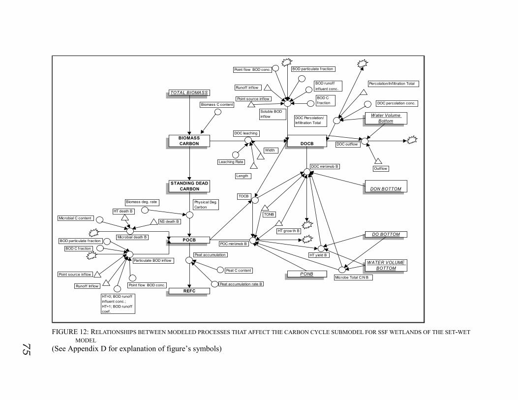
75

TOTAL BIOMASS

Water Volume Bottom

BIOMASS CARBON DOCB

STANDING DEAD CARBON DON BOTTOM

DO BOTTOMPOCB

WATER VOLUME BOTTOM

PONB

REFC

Outf low

DOC outf low

Soluble BOD inf low

BOD C f raction

BOD runof f

inf luent conc.

BOD particulate f raction

Runof f inf low


Point f low BOD conc.

DOC leaching

Leaching Rate

Biomass C content

Physical Deg. Carbon

Biomass deg. rate

Microbial death B

Microbial C content

HT death B

NS death B

Particulate BOD inf low

BOD C f raction

HT=0; BOD runof f inf luent conc.;HT=1; BOD runof f coef .

BOD particulate f raction


Point f low BOD conc.Runof f Inf low

Peat accumulation

Peat C content

Peat accumulation rate B

DOC min\imob B

POC min\imob B

TOCB

TONB

HT grow th B

HT yield B

Microbe Total C:N B

Percolation/Inf iltration Total

DOC percolation conc.

DOC Percolation/Inf iltration Total

Length

Width

FIGURE 12: RELATIONSHIPS BETWEEN MODELED PROCESSES THAT AFFECT THE CARBON CYCLE SUBMODEL FOR SSF WETLANDS OF THE SET-WET

MODEL


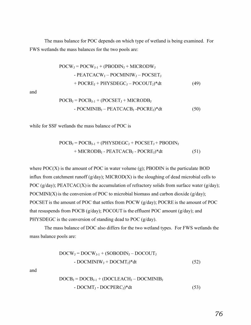
76

The mass balance for POC depends on which type of wetland is being examined. For

FWS wetlands the mass balances for the two pools are:

POCWJ = POCWJ-1 + (PBODINJ + MICRODWJ

- PEATCACWJ – POCMINIWJ – POCSETJ

+ POCREJ + PHYSDEGCJ – POCOUTJ)*dt (49)

and

POCBJ = POCBJ-1 + (POCSETJ + MICRODBJ

- POCMINIBJ – PEATCACBJ -POCREJ)*dt (50)

while for SSF wetlands the mass balance of POC is

POCBJ = POCBJ-1 + (PHYSDEGCJ + POCSETJ + PBODINJ

+ MICRODBJ - PEATCACBJ - POCREJ)*dt (51)

where POC(X) is the amount of POC in water volume (g); PBODIN is the particulate BOD

influx from catchment runoff (g/day); MICROD(X) is the sloughing of dead microbial cells to

POC (g/day); PEATCAC(X) is the accumulation of refractory solids from surface water (g/day);

POCMINI(X) is the conversion of POC to microbial biomass and carbon dioxide (g/day);

POCSET is the amount of POC that settles from POCW (g/day); POCRE is the amount of POC

that resuspends from POCB (g/day); POCOUT is the effluent POC amount (g/day); and

PHYSDEGC is the conversion of standing dead to POC (g/day).

The mass balance of DOC also differs for the two wetland types. For FWS wetlands the

mass balance pools are:

DOCWJ = DOCWJ-1 + (SOBODINJ – DOCOUTJ

- DOCMINIWJ + DOCMTJ)*dt (52)

and

DOCBJ = DOCBJ-1 + (DOCLEACHJ – DOCMINIBJ

- DOCMTJ - DOCPERCJ)*dt (53)

77

while for SSF wetlands, the mass balance is:

DOCBJ = DOCBJ-1 + (SOBODINJ + DOCLEACHJ

- DOCMINIBJ – DOCOUTJ)*dt (54)

where DOC(X) is the amount of DOC in the water volume (g); SOBODIN is the soluble BOD

influx from catchment runoff (g/day); DOCOUT is the effluent DOC (g/day); DOCMINI(X) is

the conversion of DOC to microbial biomass and carbon dioxide (g/day); DOCMT is the amount

of DOC that diffuses at the interface (g/day); DOCLEACH is the leaching of DOC from standing

dead (g/day); and DOCPERC equals the amount of DOC lost/gained from infiltration/percolation

(g/day).

Since the model is designed for NPS pollutants, a general assumption of the chemical

composition of the material coming into the wetland system is difficult to determine. This value

is site-specific and can be estimated with the approach presented by McCarty (1975).

Microbial sloughing contributes to the POC content and is the product of the microbial C

content and the sum of heterotroph and autotroph death. Microbes are not considered to be a part

of POC until they die and are accounted for in the bacteria counts. It is assumed that microbial

death contributes only to POC, not DOC, since most microbes in wetland systems are associated

with plant litter and soil organic matter. Particulate BOD inflow is determined as:

PBODINJ = 1.4 * BODPFRAC * BODCFRAC * (BODINFCO

* WATINPUTJ + APFLOW * BODCONC) (55)

where PBODIN is the particulate BOD flux from waste additions (g C/day); BODPFRAC is the

fraction of influent BOD that is in particulate form (g part. BOD5/g total BOD5); BODCFRAC is

the fraction of C in influent BOD (g C/g BOD5); BODINFCO is the BOD5 concentration in

catchment runoff (mg BOD5/l); WATINPUT is the amount of catchment runoff (m3); APFLOW

is the amount of point flow contributions (m3); and BODCONC is the BOD5 concentration in

point source (mg BOD5/l). Five day BOD is converted to ultimate BOD assuming k=0.25

(Tchobangolous and Burton, 1991).

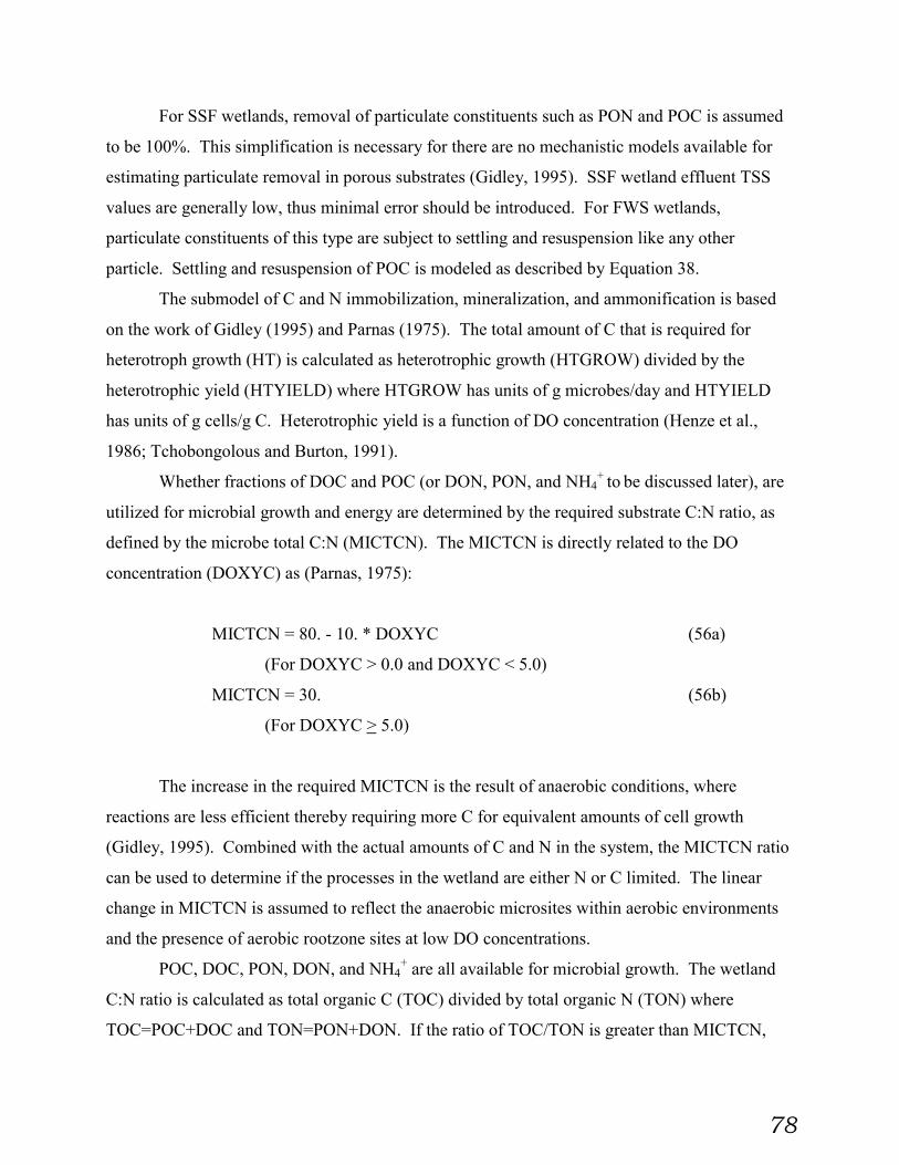
78

For SSF wetlands, removal of particulate constituents such as PON and POC is assumed

to be 100%. This simplification is necessary for there are no mechanistic models available for

estimating particulate removal in porous substrates (Gidley, 1995). SSF wetland effluent TSS

values are generally low, thus minimal error should be introduced. For FWS wetlands,

particulate constituents of this type are subject to settling and resuspension like any other

particle. Settling and resuspension of POC is modeled as described by Equation 38.

The submodel of C and N immobilization, mineralization, and ammonification is based

on the work of Gidley (1995) and Parnas (1975). The total amount of C that is required for

heterotroph growth (HT) is calculated as heterotrophic growth (HTGROW) divided by the

heterotrophic yield (HTYIELD) where HTGROW has units of g microbes/day and HTYIELD

has units of g cells/g C. Heterotrophic yield is a function of DO concentration (Henze et al.,

1986; Tchobongolous and Burton, 1991).

Whether fractions of DOC and POC (or DON, PON, and NH4+

to be discussed later), are

utilized for microbial growth and energy are determined by the required substrate C:N ratio, as

defined by the microbe total C:N (MICTCN). The MICTCN is directly related to the DO

concentration (DOXYC) as (Parnas, 1975):

MICTCN = 80. - 10. * DOXYC (56a)

(For DOXYC > 0.0 and DOXYC < 5.0)

MICTCN = 30. (56b)

(For DOXYC > 5.0)

The increase in the required MICTCN is the result of anaerobic conditions, where

reactions are less efficient thereby requiring more C for equivalent amounts of cell growth

(Gidley, 1995). Combined with the actual amounts of C and N in the system, the MICTCN ratio

can be used to determine if the processes in the wetland are either N or C limited. The linear

change in MICTCN is assumed to reflect the anaerobic microsites within aerobic environments

and the presence of aerobic rootzone sites at low DO concentrations.

POC, DOC, PON, DON, and NH4+ are all available for microbial growth. The wetland

C:N ratio is calculated as total organic C (TOC) divided by total organic N (TON) where

TOC=POC+DOC and TON=PON+DON. If the ratio of TOC/TON is greater than MICTCN,

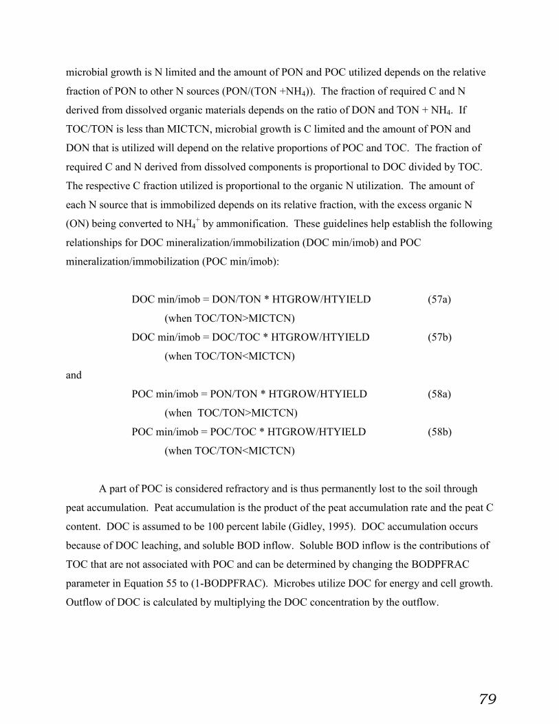
79

microbial growth is N limited and the amount of PON and POC utilized depends on the relative

fraction of PON to other N sources (PON/(TON +NH4)). The fraction of required C and N

derived from dissolved organic materials depends on the ratio of DON and TON + NH4. If

TOC/TON is less than MICTCN, microbial growth is C limited and the amount of PON and

DON that is utilized will depend on the relative proportions of POC and TOC. The fraction of

required C and N derived from dissolved components is proportional to DOC divided by TOC.

The respective C fraction utilized is proportional to the organic N utilization. The amount of

each N source that is immobilized depends on its relative fraction, with the excess organic N

(ON) being converted to NH4+ by ammonification. These guidelines help establish the following

relationships for DOC mineralization/immobilization (DOC min/imob) and POC

mineralization/immobilization (POC min/imob):

DOC min/imob = DON/TON * HTGROW/HTYIELD (57a)

(when TOC/TON>MICTCN)

DOC min/imob = DOC/TOC * HTGROW/HTYIELD (57b)

(when TOC/TON<MICTCN)

and

POC min/imob = PON/TON * HTGROW/HTYIELD (58a)


POC min/imob = POC/TOC * HTGROW/HTYIELD (58b)


A part of POC is considered refractory and is thus permanently lost to the soil through

peat accumulation. Peat accumulation is the product of the peat accumulation rate and the peat C

content. DOC is assumed to be 100 percent labile (Gidley, 1995). DOC accumulation occurs

because of DOC leaching, and soluble BOD inflow. Soluble BOD inflow is the contributions of

TOC that are not associated with POC and can be determined by changing the BODPFRAC

parameter in Equation 55 to (1-BODPFRAC). Microbes utilize DOC for energy and cell growth.

Outflow of DOC is calculated by multiplying the DOC concentration by the outflow.

80

7. Nitrogen Submodel:

Processes that are always modeled by the N submodel include ammonification (W/B),

immobilization (W/B), nitrification (W/B), denitrification (W/B), and peat accumulation (W/B).

As stated before, there are flags that signify whether ammonia volatilization (W), atmospheric

deposition (W) and N fixation (W) will also be included in the overall N cycle modeling. These

are user-defined options, whereby all or none of the processes have to be included in the

simulation. Sorption of NH4+ is not modeled as it is assumed that sorbed NH4

+ is still available

to attached microbes. The state variables include dissolved organic N (DON; W/B), particulate

organic N (PON; W/B), NH3 and NH4+-N (NH4; W/B), nitrate N (NO3; W/B), immobilized N

(W/B), and refractory N (Figures 13 and 14).

Influent DON enters the wetland through catchment runoff, point source inflow, percolation,

and atmospheric deposition (dry and wet):

DONINJ = (1 – ONPARTF) * WATINPUTJ * ORGNINCJ

+ APFLOW * DONCONC (59)

where DONIN is the incoming DON to wetland (g N/day); ONPARTF is the fraction of organic

N in particulate form (g PON/g TON); ORGNINC is the influent ON from catchment runoff (mg

ON-N/L); and DONCONC is the ON concentration from point sources (mg ON-N/L).

If the atmospheric deposition option is chosen and there is no precipitation, then the total

dry deposition for that day is the dry deposition rate (g DON/ m2) multiplied by the wetland

surface area. If precipitation does occur, then the input to the wetland is the total precipitation

amount multiplied by the concentration of DON in the rain.

Dissolved organic N also accumulates by leaching of N from the standing dead, due to

the physical degradation of standing dead biomass. It is assumed that accumulation occurs based

on a constant proportion of C to N in the plant biomass. Dissolved organic N leaching is

calculated as the product of the DOC leaching rate and the biomass C:N ratio (BIOMASS C:N).

Dissolved organic N outflow is determined by multiplying the wetland DON concentration by

the outflow. As previously described, a part of DON is reincorporated into microbial biomass

during the degradation of organic C; while the rest is wasted as ammonium. These relations are

as follows:

81

WATER VOLUME BOTTOM

NO3 SURFACE

IMMOBILIZED N SURFACE

NH4 SURFACE

NO3 BOTTOMWater Surface

Water Bottom


DOC SURFACE

NH4 BOTTOM

DON SURFACE

DON BOTTOM

Water Surface

Water Bottom

NH4 SURFACE DON SURFACEIMMOBLIZED N

SURFACEPON SURFACE

AnaHT NO3 yield B

Outflow

NO3 inf luent

HT=0; NO3 runof f

influent conc.;HT=1; NO3 runof f

coef f.

Nitrif ication B

NS Yield B

NH4 influent

DON influent

HT=0; Inf luent runof f

ON conc.;

HT=1; ON runoff coef f.

ON particulate fraction

runoff inflow

Point source inflow

HT=0; inf luent

runoff NH4 conc.HT=1; NH4 runoff

coef f.

Point NH4 conc.

Point NO3 conc

Dry A.D. NO3

Wet A.D. NO3

Length

Width

Direct precip.

A. D. flag

Point ON conc.

Wet A.D.

Dry A.D.

Wet A.D. DONDry A.D. DON

HT yield B

N leaching

Biomass C:N

DOC leaching

NO3 outf low

Volatization

pH factorpH

Nitrogen Fixation

Nitrogen fixation rate

Width

Length

Denitif ication B

Anaerobic HT grow th W

HT NO3 yield W

Nitrif ication W

NS Yield W

biomass grow thNS grow th W

Biomass C:N

H

nitrate uptake W

ammonium uptake W

PON

Microbial N content

HT NH4 immob. W

HT g

Plant

Plant up division

HT yield W

TON W

DON immobilization W

TOCW

Microbe Total C:N W

HT grow th W TONWTONW & NH4W

Microbial N Content

HT NH4 immob. W

DON ammoniafication W

DON ammoniafication B

TON B

Outflow

DON outflow

NH4 outflow

Volatilization rate

NO3 mass

transfer

NO3 MT coef.

Surface

Area

NH4 MT coef .NH4 MT

Surface area

DON mass transfer

DON MT coef .

DON Perc./Inf. Conc.

DON Per

Perc./Inf. Total

NH4 PeInf. Co

Perc./Inf

FIGURE 13: RELATIONSHIPS BETWEEN MODELED PROCESSES THAT AFFECT THE NITROGEN CYCLE

SUBMODEL FOR FWS WETLANDS OF THE SET-WET MODEL


82

WATER VOLUME BOTTOM

POC SURFACE

IMMOBILIZED N SURFACE

PON SURFACE

POC SURFACE

NO3 BOTTOM

POC BOTTOM

IMMOBILIZED N BOTTOM

NH4 BOTTOM PON BOTTOM REFRACTORY N

DOC BOTTOMPOC BOTTOM

DON BOTTOM

Water Surface

Water Bottom

NH4 BOTTOM DON BOTTOM

PON BOTTOM

PON inf luent

Peat accumulation rate W

runoff

ON Particulate fraction

HT=0; Inf luent runoff ON conc.;HT=1; ON runoff coeff .

Point source flow

Point ON conc.

Anaerobic HT grow th BO3 yield B

Nitrif ication B

NS Yield B

biomass grow thNS grow th B

Biomass C:N

HT death B NS death B physical degradation C

HT grow th B

nitrate uptake B

ammonium uptake B

d B

DON immobilization B

TOCB

Microbe Total C:N B

PON immobilization B

PON ammonif ication B

Microbial N content

HT grow th B

death BTONB & NH4B

A. D. flag Dry A.D. PON

Wet A.D. PON

Length

Width

Direct precip.

HT NH4 immob. B

TOCBTONB

Microbe Total C:N B

HT yield

HT grow th B TONBTONB & NH4B

Microbial N Content

HT NH4 immob. B

fication B

Biomass C:N

HT death W NS death W physical degradation C

HT grow th WPON immobilization

PON ammonif ication W

death TONW & NH4W

mmob. W

TOCBTONW

Microbe Total C:N

HT yield WHT grow th W

Plant up division

tion B

Peat N content


PON resuspension

PON falling rate

HT

HI

PON size

PON resusp. crit. vel.

MANNC

HB

Water velocity

PON settling

PON resusp. thick.

PON resusp rate

oef.


DON Perc./Inf il.

Perc./Inf. Total

NH4 Perc./Inf. Conc.

NH4 Perc./Inf il. Perc./Inf. Total

NO3 Perc./Inf. Conc.

NO3 Perc./Inf il.

Perc./Inf. Total

FIGURE 13 (CONT.): RELATIONSHIPS BETWEEN MODELED PROCESSES THAT AFFECT THE NITROGEN

CYCLE SUBMODEL FOR FWS WETLANDS OF THE SET-WET MODEL


83

WATER BOTTOM

WATER VOLUME BOTTOM

NO3 BOTTOM


NH4 BOTTOM

WATER BOTTOM

DOC BOTTOM

DON BOTTOM

NH4 BOTTOMWATER BOTTOM

Denitrification B

Anaerobic HT growth BHT NO3 yield B

Outflow

NO3 influentHT=0; NO3 runoff influent conc.;HT=1; NO3 runoff coeff.

Nitrification B

NS Yield B

NH4 influent

DON influent

HT=0; Influent runoff ON conc.;HT=1; ON runoff coeff.

ON particulate fraction

runoff inflow

Point source inflow

HT=0; influent runoff NH4 conc.HT=1; NH4 runoff coeff.

Point NH4 conc.

biomass growthNS growth B

Biomass C:N

HT

nitrate uptake B

ammonium uptake B

Point NO3 conc

Dry A.D. NO3

Wet A.D. NO3

Length

Width

Direct

A. D. flag

Point ON conc.

Wet A.D. NH4

Dry A.D. NH4

Wet A.D. DON

Dry A.D. DON

DON ammonification

HT yield B

NH4 outflow

DON outflow


TON BTOCB

Microbe Total C:N B

N leaching

Biomass C:N

DOC leaching

PON

Microbial N content

NO3 outflow

HT NH4 immob. B

HT growth B T

HT NH4 immob. B

Volatization

Volatization rate

pH factor

pH

Nitrogen Fixation

Nitrogen fixation rate

Width

Length

Plant up division

Perc./Inf. Total

NO3 Percolation/Infiltration Conc.

NO3 Perc./Infil.

Perc./Inf. Total

NH4 Perc./Inf. Conc.

NH4 Perc./Infil.

Perc./Inf. Total

DON Perc./Infil.


FIGURE 14: RELATIONSHIPS BETWEEN MODELED PROCESSES THAT AFFECT THE NITROGEN CYCLE SUBMODEL FOR SSF WETLANDS OF THE SET-WET MODEL


84

WATER VOLUME BOTTOM

POC BOTTOM


PON BOTTOM REFRACTORY N

POC BOTTOM

DOC BOTTOM

WATER VOLUME BOTTOM

NH4 BOTTOM DON BOTTOM

PON BOTTOM

PON influent

Peat N content


catchment runoff inflow ON Particulate fraction

HT=0; Influent runoff ON conc.;HT=1; ON runoff coeff.

Point source flow

Point ON conc.

HT growth B

w

biomass growthBiomass C:N

HT death B NS death B physical degradation C

HT growth B

ake B

DON outflow


Outflow

be Total C:N B

PON immobilization B

PON ammonification B

bial N content

HT growth B

death BTONB & NH4B

A. D. flag

Dry A.D. PON

Wet A.D. PON

Length

Width

Direct precip.

HT NH4 immob. B

TOCBTONB

Microbe Total C:N B

HT yield B

T growth BTONBTONB & NH4B

Microbial N Content

HT NH4 immob. B

Perc./Inf. Total

Perc./Inf. Total

FIGURE 14 (CONT.): RELATIONSHIPS BETWEEN MODELED PROCESSES THAT AFFECT THE NITROGEN CYCLE SUBMODEL FOR SSF WETLANDS

OF THE SET-WET MODEL


85

DONIM = DON/ (TON+NH4) * MICRONC *HTGROW (60a)


DONIM = DOC/TOC * (MICRONC * HTGROW - HTNH4IM) (60b)


PONIM = PON/(TON+NH4)*MICRONC*HTGROW (61a)


PONIM = POC/TOC *(MICRONC * HTGROW - HTNH4IM) (61b)


HTNH4IM = MICRONC *HTGROW *NH4 / (TON +NH4) (62)

DONAM = 0 (63a)

(when TOC/TON > MICTCN or DOC < 0.1)

DONAM = DOC/TOC * HTGROW/HTYIELD (63b)

*DON/DOC – DONIM

(when TOC/TON < MICTCN)

PONAM = 0 (64a)

(when TOC/TON >MICTCN or POC < 0.1)

PONAM = POC/TOC * HTGROW/HTYIELD * PON/POC (64b)

-POC/TOC * (MICRONC * HTGROW - HTNH4IM)

(when TOC/TON < MICTCN)

where DONIM is DON immobilization (g N/day); DONAM is DON ammonification (g N/day);

MICRONC is the microbial N content (g N/g microbes); HTGROW equals the heterotrophic

(HT) growth rate (g microbes/day); HTYIELD is the yield of HT bacteria (g microbes/g C

degraded); HTNH4IM is the NH4 utilized by HT bacteria during organics degradation (g NH4+-

N); PONIM is PON immobilization (g N/day); and PONAM is PON ammonification (g N/day).

86

Another source of DON to the wetland system is N fixation. N fixation is assumed to

occur at a constant user provided rate. Mass transfer of DON between the surface and bottom of

the wetland is modeled as discussed previously (Equation 39).

Particulate organic N dynamics are similar to those for DON, except that PON is

assumed to also accumulate in peat as refractory N. Peat N accumulation is the product of the

peat accumulation rate and the peat N content. Particulate organic N outflow is zero for SSF

wetlands and is calculated as the product of the wetland concentration and the outflow.

NH4+ and NH3 are referred to as NH4 only because at neutral pH, the predominate form is

NH4+. NH4

+ accumulates through NH4+ influent (catchment, point, percolation, and

atmospheric), and PON and DON ammonification. NH4+ influent is modeled similar to DON

(Equation 60), while PON and DON ammonification are modeled as previously discussed

(Equations 64 and 65). Plant and microbial uptake, NH4+ effluent, infiltration and nitrification

all decrease NH4+ amounts in the wetland. NH4

+ uptake is the sum of the plant uptake (minus

nitrate uptake), and microbial uptake (the sum of HTNH4IM and the product of Nitrosomonas

bacteria growth and microbial N content). Biomass is assumed to prefer NO3- rather than NH4

+

as a N source, thus NH4+ utilization only occurs when NO3

- amounts are insufficient. NH4+ is

used by autotrophic bacteria as an electron source converting it to nitrate through nitrification,

which is modeled as the quotient of Nitrosomonas growth and Nitrosomonas yield.

Volatilization is an optional model component that affects ammonium concentrations.

Volatilization is modeled as a first order equation with an included pH factor. Mass transfer

occurs as a function of the concentration gradient (Equation 39).

Immobilized N is the sum of DON and PON immobilization, NO3- uptake and NH4

+

uptake. Immobilized N eventually returns to PON through the death of microbes and biomass.

These values are the product of the respective death rates and N contents as discussed in the

microbial and C submodels.

The last N pool is NO3- (NO3). Influent concentrations and mass transfer are modeled in

the same manner as other dissolved N pools. Nitrate pool increases are due to nitrification and

influent contributions, and is decreased by plant uptake and denitrification. Nitrate uptake is

modeled as the product of biomass growth and biomass C:N ratio. Nitrate outflow is the product

of the wetland outflow and wetland nitrate concentration. Anaerobic heterotrophs use NO3- as an

electron acceptor to convert the NO3- to N2 gas, which is eventually lost to the atmosphere. It is

87

assumed that the movement of the N2 gas from the soil system is instantaneous, as the diffusion

of the product is not modeled. Denitrification is modeled as the quotient of anaerobic

heterotroph growth and heterotroph NO3- yield. Other intermediates such as NO and N2O are

produced by microbes, but are not considered in the simulation.

8. Dissolved Oxygen Submodel:

The oxygen budget (Figures 15 and 16) consists of the single state variable, DO (W/B).

Oxygen is added to the wetland through influent runoff, influent point sources, DO

concentrations in precipitation, percolation, by plants and re-aeration. Re-aeration with the

atmosphere is modeled only for FWS wetlands as it is assumed that oxygen transfer with the

atmosphere is negligible in SSF systems because the water surface is below the substrate. The

mass balance for DO in the FWS wetland surface is:

DOXYWJ = DOXYWJ-1 + (DOINFJ + MTDOXYJ

+ MTFWSJ – HTRESPWJ – NSRESPWJ - DOOUTJ)*dt (65)

for FWS wetland bottoms:

DOXYBJ = DOXYBJ-1 + (BIOFLUXB – DOPERCJ

-HTRESPBJ – NSRESPBJ - MTDOXYJ)*dt (66)

and for SSF wetlands:

DOXYBJ = DOXYBJ-1 + (DOINFJ – DOPERCJ

BIOFLUXB – HTRESPBJ - NSRESPBJ)*dt (67)

where DOXY(X) is the amount of DO in water volume (g); DOINF is the oxygen additions from

runoff and point inflow (g/day); MTDOXY is the diffusion of DO from one pool to the other

(g/day); MTFWS is the DO re-aeration from atmosphere (g/day); HTRESP(X) is the oxygen loss

by heterotroph growth (g/day); NSRESP(X) is the oxygen loss due to autotroph growth (g/day);

DOOUT is the effluent DO (g/day); DOPERC are additions from percolation (g/day); and

BIOFLUXB is the oxygen flux from rootzone aeration by plants (g/day).

88

DISSOLVEDOXYGENSURFACE

WATERVOLUME

SURFACE

WATERVOLUMEBOTTOM

DISSOLVEDOXYGENBOTTOM

HT respiration W NS respiration W

Outf low

Aerobic HT

growth W

HT DO

y ield WNS DO

y ield W

NS growth W

DO outf low

Runoff inf low

Point f low DO conc.


Precipitation input

At. DO conc.

Inf luent DO

Surf ace area

Biomass oxy genation rate

Biomass f lux

HT respiration B NS respiration B

Aerobic HT

growth B

HT DO

y ield WNS DO

y ield B

NS growth B

DO mass transf er

Reairation

Parameters;

Reairc,Reairm,

Reairn,

Doxy csat

HT=0, inf luent DO conc.;

HT=1, DO runoff conc.

DO MT coef .

DO Percolation/

Inf iltration

DO Percolation/

Inf iltration Conc.

Percolation/

Inf iltration Total

FIGURE 15: RELATIONSHIPS BETWEEN MODELED PROCESSES THAT AFFECT THE OXYGEN CYCLE

SUBMODEL FOR FWS WETLANDS OF THE SET-WET MODEL


89

DISSOLVEDOXYGENBOTTOM

WATERVOLUMEBOTTOM

Surface areaBiomass oxygenation rate

Biomass flux

HT respiration W NS respiration W

OutflowAerobic HTgrowth W

HT DOyield W

NS DOyield W

NS grow th W

DO outflow

HT=0, influent DO conc.;HT=1, DO runoff conc.

Runoff inflow

Point f low DO conc.


Precipitation input

At. DO conc.

Influent DO

DO Percolation/Infiltration

DO Percolation/Infiltration Conc.

Percolation/Infiltration Total

FIGURE 16: RELATIONSHIPS BETWEEN MODELED PROCESSES THAT AFFECT THE OXYGEN CYCLE SUBMODEL FOR SSF

WETLANDS OF THE SET-WET MODEL (SEE APPENDIX D FOR EXPLANATION OF FIGURE’S SYMBOLS)

90

Re-aeration to the wetland is modeled using a general two-film theory that is based on

mass transfer. The mass transfer of oxygen from air to water can be presented as (Jorgensen,

1983):

( )CCV

AK

dt

dCS

L −= * (68)

where KL is the mass transfer coefficient (m/day); A is the surface area through which diffusion

takes place (m2); V is the volume of water being re-aerated (m3); Cs is the oxygen saturation

concentration (g/m3); and C is the oxygen concentration in surface water volume (g/m3).

Biomass flux is the product of the biomass oxygenation rate and the wetland surface area.

It is assumed that there is a uniform vegetation stand throughout the wetland system and that

plants transport of oxygen to the wetland bottom occurs at a constant rate through the growing

season. This assumption is based on the theory that processes such as Knudsen diffusion are

responsible for rootzone aeration (Grosse, 1989). The biomass oxygenation rate is linearly

increased from zero to the maximum biomass oxygenation rate starting from the first day of the

growing season and decreasing linearly to zero at the end of the growing season. Although not

linked through any proportionality ratios, the oxygenation rate is ramped to correspond with the

vegetative growth model.

Chemical oxidation of reduced iron and manganese, and autotrophic and heterotrophic

respiration are two of the processes that consume dissolved oxygen in a wetland (Reddy and

Patrick, 1983). Heterotroph (HTRESP) and Nitrosomonas (NSRESP) respiration are modeled as

proportional to microbial growth:

HTDOY

AEHTGRWHTRESP = (69)

NSDOY

ANHTGRWNSRESP = (70)

where HTRESP is the oxygen loss due to heterotrophic growth (g O2/day); AEHTGRW is the

growth of aerobic heterotrophs (g microbes/day); HTDOY is the oxygen yield of aerobic

91

heterotrophs (g microbes/g O2); NSRESP is the oxygen loss due to Nitrosomonas growth (g

O2/day); ANHTGRW is the growth of anaerobic autotrophs (g microbes/day); and NSDOY is

the oxygen yield of Nitrosomonas bacteria (g microbes/g O2).

Most constructed wetlands have gravel substrates and secondary wastewater additions are

generally aerobic; therefore reduced iron, manganese and sulfide concentrations are considered

negligible. The dissolved oxygen outflow from the system is the product of the wetland DO

concentration and the effluent volume from the system.

9. Bacteria Submodel:

The bacteria submodel accounts for the microbial growth and associated activities in the

model. To simplify the description, the model is described according to the natural breakdown

between autotrophic (AT) and heterotrophic (HT) bacteria.

a. Autotrophic Dynamics

The state variable NITROSO (NS, W/B) represents the AT population within the

wetland. Although there are other AT species that carry out nitrification, Nitrosomonas and

Nitrobacter are the dominant species responsible for the rate limited reaction (Wheaton et al.,

1991). Changes in the population of NS are due to NS growth and NS death (Figures 17 and 18).

Growth rate of NS is described using Monod dual substrate limitation kinetics (Gidley,

1995):

+

+

=DONH KDO

DO

KNH

NH**

44

4maxµµ (71)

where µ is the actual NS specific growth rate (day-1); µmax is the NS maximum growth rate

(day-1); NH4+

is the ammonium concentration (mg/L); KNH4 is a NS NH4+ half saturation

constant (mg/L); DO is the wetland dissolved oxygen concentration (mg/L); and KDO is the NS

DO half saturation constant. This expression modifies the NS growth rate when oxygen (the

electron acceptor) or ammonium (the electron donor) is limiting.

92

NITROSOMONAS SURFACE

NH4 SURFACE


DISSOLVED OXYGEN SURFACE

NS grow th W NS death W

NS Temp. Factor W

NS max. grow thrate W NS DO

half sat. con. W

NS NH4 half sat.con. W

Water Temp. W

NS death rate W

FIGURE 17: RELATIONSHIPS BETWEEN MODELED PROCESSES THAT AFFECT THE AUTOTROPHIC BACTERIA

CYCLE IN FWS WETLAND SURFACE WATER


NITROSOMONAS BOTTOM

NH4 BOTTOM

WATER VOLUME BOTTOM

DISSOLVED OXYGEN BOTTOM

NS grow th B NS death B

NS Temp. Factor B

NS max. grow thrate B NS DO

half sat. con. B

NS NH4 half sat.con. B

Water Temp. B

NS death rate B

FIGURE 18: RELATIONSHIPS BETWEEN MODELED PROCESSES THAT AFFECT THE AUTOTROPHIC BACTERIA

CYCLE IN FWS AND SSF WETLAND SUBSTRATE


93

Monod models are steady state and do not describe microbial growth well in unsteady

conditions (Boyd, 1978). Benefield and Molz (1984) used the Monod model to develop a

biofilm model for an idealized plate assuming pseudo steady state conditions. Gidley (1995)

also assumed pseudo steady state conditions were adequate for Monod kinetics in wetlands.

Besides substrate limitations, temperature and pH also limit microbial growth. The

optimum temperature range for NS is from 15 to 35 °C (Reddy and Patrick, 1983; Wheaton et

al., 1991), and while growth still occurs outside of this range, it is at a reduced rate. To account

for these temperature effects, the NS temperature factor is included. In the optimum temperature

range, the temperature factor equals 1.0. The factor value linearly decreases to 0 °C (the lower

limit) and to 40 °C (upper limit), once outside of the optimum range. Fyock (1977), and Reddy

and Patrick (1983) have reported that the optimum pH range for NS growth is 6-9. Wetlands

tend to drive pH toward neutrality (pH = 7), therefore a pH factor is not included. NS growth is

calculated by:

1** −= jj SNITRSOMONANSTEMPFNSGROW µ (72)

where NSGROW is the amount of NS growth (g microbes); NSTEMPF is the NS temperature

factor; and NITROSOMONAS is the amount of NS microbes (g microbes). Since there is little

information concerning the factors controlling microbial die-off, it is modeled as a first order

reaction (Equation 22).

b. Heterotrophic Dynamics

Heterotrophic (W/B) dynamics is also modeled in the bacteria submodel (Figures 19 and

20). Monod kinetics is used to model the changes in microbial growth rate caused by substrate

limitations. For HT bacteria, the electron acceptor is either oxygen or NO3- while the electron

donors are the C compounds in the system. Heterotrophs can use electron acceptors other than

oxygen, including NO3-, sulfate, iron and manganese (Gidley, 1995); however, only NO3

- is

modeled and is assumed to be the only other available electron acceptor when DO concentrations

drop below 1-2 mg/L.

94

HETEROTROPHS SURFACE

NO3 SURFACE


DISSOLVED OXYGEN SURFACE

HT grow th W HT death W

Aerobic HT grow th W

HT temp. fac. W

Water temp. W

Aerobic max.grow th rate W

HT organics half sat. con. W

Anaerobic HT grow th W

HT DO half sat constant W

Anaerobe fraction W

Anaerobic max. grow th rate W

HT NO3 halfsat. con. W

HT death rate W

TOC

FIGURE 19: RELATIONSHIPS BETWEEN MODELED PROCESSES THAT AFFECT THE HETEROTROPHIC

BACTERIA CYCLE IN FWS WETLAND SURFACE WATER


HETEROTROPHS BOTTOM

NO3 BOTTOM

WATER VOLUME BOTTOM

DISSOLVED OXYGEN BOTTOM

HT grow th B HT death B

Aerobic HT grow th B

HT temp. fac.

Water temp.

Aerobic max.grow th rate B

HT organics half sat. con. B

Anaerobic HT grow th B

HT DO half sat constant B

Anaerobe fraction B

Anaerobic max. grow th rate B

HT NO3 halfsat. con. B

HT death rate B

TOC

FIGURE 20: RELATIONSHIPS BETWEEN MODELED PROCESSES THAT AFFECT THE HETEROTROPHIC

BACTERIA CYCLE IN FWS AND SSF WETLAND SUBSTRATE


95

HT bacteria are facultative, meaning they can survive under both aerobic or anaerobic

conditions. SET-WET determines the fraction of the HT bacteria which utilize either aerobic or

anaerobic conditions based on the DO concentrations in the system (Gidley, 1995):

)75.0*(*8.0 DOXYCANFRAC = (73a)

(when 0.0 < DOXYC < 8.0)

ANFRAC = 0.2 (73b)

(when DOXYC > 8.0)

where ANFRAC is the anaerobic fraction of HT bacteria; and DOXYC is the DO concentration

(mg/L). The ANFRAC value is multiplied by the total HT bacteria amounts in the system to

determine the amount of aerobic and anaerobic bacteria that are present in the wetland. Bacteria

which utilize aerobic or anaerobic conditions always exist due to the presence of anaerobic

microsites under anaerobic conditions and aerobic microsites in the root zones under anaerobic

conditions (Gidley, 1995). Denitrification can even occur in aerobic wetland systems as

anaerobic microsites are present, and aerobes receive the necessary oxygen to survive due to

plant root diffusion.

The Monod models used for the HT bacteria are:

+

+

=DOTOC

AHAH KDO

DO

KTOC

TOC**max,µµ (74)

+

+

=DO

DO

TOCANHANH KDO

K

KTOC

TOC**max,µµ (75)

where µmaxis the maximum growth rate (day-1); TOC is the total organic C concentration (mg/L);

KTOC is the HT organics half saturation constant (mg/L); DO is the dissolved oxygen

concentration (mg/L); KDO is the HT DO half saturation constant (mg/L); AH are aerobic

heterotrophs; and ANH are anaerobic heterotrophs.

The same optimum temperature and pH rules apply to HT bacteria, as they did for the AT

bacteria. Total HT growth is the sum of the aerobic HT and anaerobic HT growth. The HT

96

growth and death are modeled in the exact manner as the AT bacteria, with the differing

respective parameter values.

10. Sediment Submodel:

The sediment cycle simulates sediment particles and any other desired suspended solid in

the wetland system (Figure 21). As stated earlier, the sediment model does not work in

conjunction with the SSF wetland simulation. For the SSF system, it is assumed that the

retention of particulates in the system is 100%, yet there is no account to the loss in porosity for

the wetland gravel substrate. Between season periods, there is an ability to change the porosity

values in the SSF system. If the system did have high loading of sediment to the system, the

model may have difficulty in modeling the NCOB cycle in the SSF system due to the clogging of

the wetland substrate. It is advised that the SSF system be used in conjunction with another

BMP designed to lower sediment concentrations, such as a detention basin, if using a SSF

system to control NPS pollution, to prevent clogging of the SSF wetland substrate.

The sediment model has been designed to accept up to five particle size categories. Each

category requires inputs for sediment diameter (SEDSIZE, mm), fall rate (SEDFALL, m/s),

initial amount in the water surface (SEDINITW, g), initial amount in the wetland bottom

(SEDINITB, g), and the percentage of the total incoming amount based on weight (SEDPER).

The final input category may be used to represent the organic suspended solids in the wetland

system. All organic material must be represented in this single category, as there is an associated

decomposition component for the final category. The decomposition component in the sediment

submodel does not run concurrently with the NCOB cycle. Decomposition is not modeled based

on the bacterial consumption modeled in the NCOB cycle, but with a simple user defined first

order rate equation. This was a necessary step to allow SET-WET the ability to simulate the

nutrient components independently.

Total incoming sediment amounts are either directly input or determined with a

combination of the SCS curve method and runoff concentrations (Equation 37). The total

incoming amount from catchment runoff and point flow is multiplied by SEDPER to determine

the incoming amounts for each respective category (SEDINW).

The balances for sediment in the wetland are (adapted from Christensen et al., 1994):

97


SEDIMENT SURFACE, X

SEDIMENT BOTTOM, X

Sed. X influent to surface

HT=1; Sed. X runoff coeff.

HT=1; runoff inflow

Sed. X influent from runoff

Point source inflow

Sed. Total point conc.

Sed. X % of Sed. Total

Outf low

Sed. X outflow

HI

HT

Outlet

Outlet = 4Pump outlet

Outlet = 1,2,3,5Outf low height

Sed. X, deposition

Sed. X falling rate

Water velocity

Sed. X, Resuspension

Sed. X, Reynold's number 2 check

Sed. X, particle diameter

Sed. X, falling rate

HI HT

Sed. X Critical Velocity

Manning's coeff. Sed. X, Reynold's number 1 check

Sed. Reynold's number 1b check

HB

Sed. Resusp. thick

Sed. Resusp. rate

Sediment Decomposition

Decomposition Rate

Physical Degradation

FIGURE 21: RELATIONSHIPS BETWEEN MODELED PROCESSES THAT AFFECT THE SEDIMENT CYCLE SUBMODEL FOR FWS WETLANDS OF THE SET-WET MODEL


98

SEDQTYWC,J = SEDQTYWC,J-1 + (SEDINWC,J

+ RESUSPC,J – SEDOUTC,J – SEDDEPC,J)*dt (76)

and

SEDQTYBC,J = SEDQTYBC,J-1 + (SEDDEPC,J

+SDECOMPSEDCAT,J – RESUSPC,J)*dt (77)

where SEDQTYW is the amount of sediment in the surface water (g), SEDQTYB is the amount

of sediment in the surface bottom (g), SEDINW is the amount of incoming sediment (g/day);

RESUSP is the amount of sediment resuspended from the surface bottom (g/day); SEDOUT is

the sediment outflow (g/day); SEDDEP is sediment deposition (g/day); C is the sediment

category; and SEDCAT is the total number of sediment categories.

Resuspension and settling of sediment particles are determined with Equation 38.

Sediment outflow is based on the fall rate and is treated like other particle constituents in the

wetland. If the fall rate exceeds the free water surface height, then sediment outflow is

considered to be zero, while for rates less than the free water surface height, a ratio of removal is

based on outflow and surface water volume.

11. Phosphorous Submodel:

The P cycle (Figure 22) is dependent on the sediment cycle, and does not operate if the

sediment cycle is not included in the simulation. The basis of the model is that all of the

suspended sediment particles provide surface area to which P can be attached and consequently,

settled, resuspended, or transformed. There are four pools for the P cycle; particulate and

dissolved for both the surface and bottom of the wetland. The budgets for the pools are as

follows (adapted from Christensen et al., 1994):

For surface water dissolved P:

DTPHOSWJ = DTPHOSWJ-1 + (DISPHOSIJ

+ PMINPPTJ – DPHOSOUTJ + PHOSMTJ)*dt (78)

99

for soil/peat water dissolved P,

DTPHOSBJ = DTPHOSBJ-1 + (PRMINBPTJ

+ PHOSPERCJ – PHOSMTJ - PHOSUPWJ)*dt (79)

for particulate P in the surface water

PPHOSC,J = PPHOSC,J-1 + (PPHOSINC,J + PPHOSRESC,J

- PMINPPC,J – PPHOSSETC,J –PPHOSOUTC,J)*dt (80)

and for bottom particulate P

BTPHOSC,J = BTPHOSC,J-1 + (PPHOSSETC,J

+ DEADPHOSC,J – PRMINBPTC,J –PPHOSRESC,J)*dt (81)

where DTPHOSW is the total dissolved P in surface water (g P); DTPHOSB is the total

dissolved P in wetland bottom (g P); PPHOS is the particulate P in surface water (g P); BTPHOS

is the particulate P in the wetland bottom (g P); DISPHOSI is the influent dissolved P (g P/day);

PMINPPT is the P mineralization from the particulate pool (g P/day); MASSTP is the mass

transfer of dissolved P (g P/day); DPHOSOUT is the effluent dissolved P outflow (g P/day);

PRMINBPT is the P remineralization from bottom particulate pool (g P/day); PPHOSRES is the

resuspension of particulate P from bottom (g P)/day; PPHOSOUT is the particulate P effluent

outflow (g P/day); PPHOSSET is the particulate P settling from surface (g P/day); and

DEADPHOS is the contribution of P from physical degradation of standing dead (g P/day).

Incoming particulate P amounts are modeled using either the Freundlich isotherm

(Equation 30), the Linear isotherm (Equation 31) or as direct input. If using either the Linear or

Freundlich isotherms, the dissolved P concentration is used to determine the particulate P

concentration. Knowing the weight of sediment, the surface area for each particle class is

determined and the particulate P is assumed to be partitioned among each particle class

100

DISSOLVED PHOSPHOROUS (DP) SURFACE

PARTICULATE PHOSPHOROUS

(PPS) SURFACE; XSEDIMENT

SURFACE, X


SEDIMENT SURFACE, X

SEDIMENT BOTTOM, X

WATER VOLUME BOTTOM

DISSOLVED PHOSPOROUS (DP) BOTTOM

PARTICULATE PHOSPHOROUS

(PPB) BOTTOM; X


Runof f inf low

HT=0, runof f DP conc.HT=1;DP runof f coef f .

Point DP conc.

DP inf luent

PPS mineralization coef f .

P minerlization f rom Sed. X

P min. total f rom Sed. Total

P reminerlization f rom Sed. X

PPB remineralization coef f .

P remin. total f rom Sed. Total

PPS,Xsettling

Sed. X., deposition

PP,X resuspensionSed. X Resuspension

Biomass Grow thBiomass Plant/Phos ratio

Plant DP uptake

DP Mass transfer

# of sed. categoriesDP mass transfer coef f .

Physical degradation

PPB f rom plant deg.

PPB ratio

Sed. X outf low

PPS outf low

PPS, x inf luent

PPS attachment ratio

runof f inf low

PPS inf luent total

point source inf low

PPS conc. In point

PPS conc. In runof f

AD=0, Freundlich K coef .

AD=0, Freundlich N coef .

AD=1, Linear partition coef .

Adsorption (AD) f lag

AD=2, PPS inf luent

Sed. X part. volume

Sed. X part surface area

Sed. X total surface area

Sed. Total total surface area

Sed. X particle #

Sed. X inf luent volumeSed. X inf luent mass

Sed. specif ic gravity

Length

Width

DP Percolation/Inf iltration Rate

Percolation/Inf iltration Total

DP Percolation/Inf iltration

FIGURE 22: RELATIONSHIPS BETWEEN MODELED PROCESSES THAT AFFECT THE PHOSPHOROUS CYCLE SUBMODEL FOR FWS WETLANDS OF THE

SET-WET MODEL


101

according to the incoming surface area ratio for the particle class, divided by the total of all

particle surface areas.

Mass transfer of dissolved P is modeled in the form of Equation 39. Mineralization and

remineralization are modeled as first order equations for each particular category of particles.

Resuspension and settling of P corresponds to the amount of sediment particles and is related to

the ratio of each category that resuspends and settles. This also applies to the attached P for P

outflow. The contributions of P made by physical degradation (DEADPHOS) is based on the

plant:phosphorous ratio (BIOMPP). The quotient of physical degradation and BIOMPP

determines DEADPHOS. As the suspended particles are broken into categories, the addition of

each category amount allows the determination of the total amounts in each pool.

12. Deltaht Submodel:

The DELTAHT submodel determines the change in height, respective to the zero datum,

of the wetland surface bottom. This applies only to FWS wetlands and is activated whenever the

sediment or N cycles are being simulated.

If only the N cycle is being modeled the changes in the wetland bottom surface height

(HT) are determined by:

( )WIDTHLENGTH

PEATDENS

PEATACRB

DELTAHT

J

*

1000*

= (82)

where DELTAHT is the change in height of the soil top layer (m); PEATACRB is the bottom

peat accumulation rate (g/day); and PEATDENS is the peat density (kg/m3). If only the sediment

cycle is being modeled the changes in HT are determined by:

( )WIDTHLENGTH

SEDSPG

SEDTOTAL

DELTAHT*

1000000*

= (83)

102

where SEDSPG is the sediment specific gravity (kg/m3), and SEDTOTAL is the total change in

sediment mass of the wetland bottom (g). If both options are activated then DELTAHT is

determined by:

WIDTHLENGTH

SEDSPG

SEDTOTAL

PEATDENS

PEATACRBJ

DELTAHT**1000

*1000

+

= (84)

13. SET-WET Flow Chart

Figure 23 shows the flow chart of the SET-WET model. However, the main program was

removed from the flow chart for sake of clarity. As Figure 7 indicates, the main program calls

every submodel and thus the number of connections required to represent these interactions

would make Figure 23 impossible to view or understand. Instead, the main program is not

shown in Figure 23, and the connections shown represent the flows from one submodel to

another without referring to the actual flow from the main program for each section.

C. MODEL DEVELOPMENT SUMMARY

The developed model, entitled SET-WET, simulates the hydrologic, N, C, bacteria, DO,

vegetative, P and sediment cycles of a wetland system. The N, C, DO, and bacteria cycles are

linked and cannot be run independently. These cycles are referred to as the NCOB cycle to

denote their dependence. The P cycle is dependent on the sediment cycle, and neither the

sediment nor P cycles may be simulated with the SSF wetland option. Any simulation run that

includes modeling the NCOB, sediment or P cycles requires that vegetative growth be simulated.

The SET-WET model is designed so that the hydrologic component may be run independently or

concurrently with any or all of the NCOB, sediment and P cycles.

The SET-WET model development was based on the work of Gidley (1995), Parnas

(1975) and Christensen et al. (1994). The SET-WET model is written in Fortran 77 to facilitate

linking with existing NPS models, such as ANSWERS. The SET-WET model is based on

options. The program is developed such that a main program calls and manages the cycles and

options that need to be simulated, based on input values. SET-WET may use two different forms

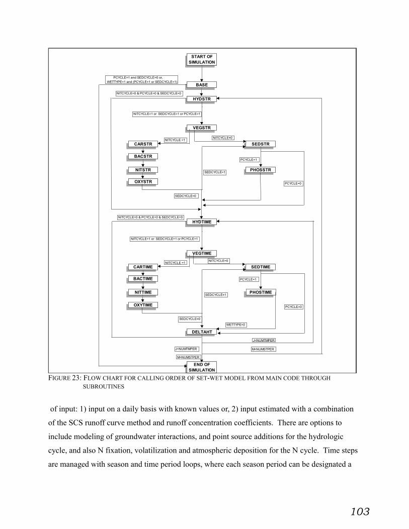
103

START OF SIMULATION

BASE

HYDSTR

VEGSTR

CARSTR SEDSTR

BACSTR

NITSTR PHOSSTR

OXYSTR

HYDTIME

VEGTIME

CARTIME SEDTIME

BACTIME

NITTIME PHOSTIME

OXYTIME

DELTAHT

END OF SIMULATION

PCYCLE=1 and SEDCYCLE=0 or, WETTYPE=1 and (PCYCLE=1 or SEDCYCLE=1)

NITCYCLE =1

PCYCLE=1

NITCYCLE=0 & PCYCLE=0 & SEDCYCLE=0

NITCYCLE=1 or SEDCYCLE=1 or PCYCLE=1

SEDCYCLE=1

PCYCLE=0

SEDCYCLE=0

NITCYCLE =1

PCYCLE=1

NITCYCLE=0 & PCYCLE=0 & SEDCYCLE=0

NITCYCLE=1 or SEDCYCLE=1 or PCYCLE=1

SEDCYCLE=1

PCYCLE=0

SEDCYCLE=0

J=NUMTMPER

J<NUMTMPER

M=NUMSTPER

M<NUMSTPER

WETTYPE=0

NITCYCLE=0

NITCYCLE=0

FIGURE 23: FLOW CHART FOR CALLING ORDER OF SET-WET MODEL FROM MAIN CODE THROUGH

SUBROUTINES

of input: 1) input on a daily basis with known values or, 2) input estimated with a combination

of the SCS runoff curve method and runoff concentration coefficients. There are options to

include modeling of groundwater interactions, and point source additions for the hydrologic

cycle, and also N fixation, volatilization and atmospheric deposition for the N cycle. Time steps

are managed with season and time period loops, where each season period can be designated a

104

certain number of daily time periods. Designed to act like a continuously stirred tank reactor, the

model assumes all incoming nutrients are evenly mixed throughout the entire volume. Dissolved

nutrient effluent concentrations from the wetland system are determined with a ratio of the

hydrologic outflow and the total amount of water volume in the system. Particulate effluent

concentrations are determined with the ratio of the fall rate and water depth in the wetland, in

conjunction with the ratio of the hydrologic outflow and the total amount of water in the wetland.

The model allows for both free water surface (FWS) and sub-surface flow (SSF) wetlands to be

modeled and, although initially developed to help with the design of constructed wetlands, SET-

WET may also be applied to model the functions of natural wetlands.

SET-WET differs from many existing wetland models in that it uses a system’s approach

and links the many interactions of the various nutrient cycles in a wetland system. It accounts

for C and N interactions, as well as for effect of DO levels upon microbial growth. It also

directly links microbial growth and death to the consumption and transformations of nutrients in

the wetland system. Many previous models have accounted for these interactions with zero and

first order rate equations, which assume that rates are dependent only on initial concentrations.

SET-WET was developed to be as general as possible, but there were assumptions made

during model development which might not apply to all wetland locations. The model assumes

that the FWS system always has free lying surface water, and that the SSF system never floods.

This may limit its ability to model extreme climactic occurrences during drought or flood

periods. It does not account for snow or snow melt, which may limit its use to warmer climate

areas. The model assumes that the dissolved and particulate concentrations in both the surface

water and substrate water are evenly mixed through the respective volumes, which is known to

not physically be the case.

Plant growth is assumed to be of constant composition throughout the wetland, and is not

limited by lack of nutrients or water supply. In addition, growth and death cannot occur at the

same time, therefore, the model does not account for turnover of plant material during the year.

Oxygen transfer by plants is considered to be constant through the growing season, and it is also

assumed that biomass and bacteria prefer NO3- rather than NH4

+. The use of a simple plant

model will affect the release rate of nutrients to the system from plant decomposition, but more

complicated plant growth model’s input requirements are too data intensive to be used.

105

Modeling of adsorption of NH4+ is not conducted as it is assumed that the amount that is

adsorbed is still available for microbial use. The model assumes that P is attached to all of the

particulates in the system based on the surface area of the particles. In addition, SSF wetland

aeration is assumed to be negligible because the water surface is below the substrate, and SSF

wetland PON and POC removal is assumed to be 100%.

In addition to assumptions made directly concerning wetland interactions and processes,

there are assumptions made by previous researchers that were incorporated into the model. The

Thornthwaite method for estimating ET assumes that the soil moisture in the area is not limiting

and that air temperature is the primary controller of ET. Another assumption is induced by using

mass transfer coefficients to model diffusion, which assumes that changes in concentrations

between the two pools (surface and substrate water) are limited to the small part of the system’s

volume connecting boundaries.

Although SET-WET does incorporate a few assumptions into model development, it still

offers the flexibility of modeling various designs for a desired wetland. However, these

assumptions are noted for the benefit of the user.

106

IV. Model Evaluation

Another objective of this study was to “evaluate the proposed model by comparing its

predictions with field data collected from representative constructed wetland site(s).” This

objective was difficult to satisfy because there are a lack of field data related to the control of

NPS pollution using FWS constructed wetlands. Wetlands have been created (Silverman, 1989;

Daukas et al., 1989; Teague et al., 1997) whose intent is to control NPS pollution, but data

collection has not included all relative parameters (NH4+, BOD5, DO, etc) for substantial time

periods (1-2 years) that would allow the use of data for calibration and validation of SET-WET.

The SET-WET model’s performance in simulating the functions of FWS wetlands was

evaluated with data collected at a wetland site located in Benton, Kentucky. This was not an

ideal data set because the Benton wetlands treat municipal waste, but there were no available

NPS pollution wetland data sets. The model’s performance for SSF wetlands was not evaluated;

however, previous research by Gidley (1995) examined SET-WET’s basic approach towards

modeling SSF wetlands. Model evaluation procedures included the calibration and validation of

the model, performing two types of statistical analyses, conducting a sensitivity analysis, and

using SET-WET to demonstrate its application for design of wetlands. Overall the model

performed well, even though the data used for evaluation were somewhat limited.

A. Model Calibration and Validation

1. Study Area

The SET-WET model was calibrated and validated with data collected from a constructed

wetland located in Benton, Kentucky. As described by Choate et al. (1990) and summarized by

Kadlec and Knight (1996), the Benton wetlands were designed to upgrade and polish municipal

effluent from an existing lagoon for 5000 people. There are three parallel wetland cells (two

FWS, one SSF) of equivalent size (333 m by 45m) located in Benton, but only one of the FWS

cells (cell 2) was used to examine SET-WET’s performance.

The wetland cell consists of substrate made of native clay and impermeable clay lining of

3 to 4.5 m thickness, which eliminated infiltration or percolation effects. It was planted with

107

Scripus cyperinus (L.) Kunth (woolgrass bulrush), Scripus validius Vahl. (softstem bulrush), and

Typha latiofolia L. (cattail). Influent and effluent samples were collected either monthly or

bimonthly for a variety of parameters. Measurements for most of the parameters were conducted

from March 30, 1998 until September 6, 1990; however, total suspended solids (TSS), and

dissolved and total P were discontinued after April 26, 1989. Listed in Table 5 is the data set

used as input for the calibration and validation of the SET-WET model.

Incoming input daily water flow, nutrient, and sediment values were determined by linear

interpolation between the monthly data points. This was the case for all daily parameters,

excluding the daily weather data such as precipitation and air and water temperature.

Precipitation and air temperature were obtained from NOAA (National Oceanographic and

Atmospheric Administration) records at a site located in Padukah, Kentucky; approximately 25

miles northeast of Benton (NOAA, 1988: NOAA, 1989). Water temperature was estimated from

a linear regression of the air temperature and measured water temperature. With the known air

temperature, the daily water temperature was determined.

2. Model Calibration:

Data for one year were used to calibrate and validate the SET-WET model. This time

period was chosen because the nutrient and hydrologic input data needed for SET-WET were

available. During this time period, only thirteen data points for the hydrologic and nutrient

TABLE 5: MEASURED INFLOW VALUES TO WETLAND CELL 2 IN BENTON, KENTUCKY USED FOR

VALIDATION AND CALIBRATION OF SET-WET MODEL.Flow DO BOD5 NH3-N NO3-NO2 Org-N TKN TSS Dis-P Tot-P

Date (m^3/d) mg/l mg/l mg/l mg/l mg/l mg/l mg/l mg/l mg/l4/27/88 213.2 2.4 30 12.0 0.02 5 17 30 3 4.55/25/88 567.9 8.1 34 12.0 0.02 8 20 49 5.5 6.86/29/88 339.0 2 18 5.2 0.02 11 16.2 63 6.8 7.87/27/88 350.4 8.3 19 3.1 0.01 12.3 15.4 110 4.1 5.68/30/88 472.5 16.8 * 20 0.1 0.09 9.9 10 5.4 9.79/28/88 403.6 2.4 14 4.1 0.01 9.6 13.7 59 5.6 5.7

10/25/88 478.0 6.2 23 9.8 0.36 7.1 16.9 54 6.611/29/88 1263.1 10.8 22 3.8 0.74 6.5 10.3 31 2.3 3.412/13/88 523.9 19.1 * 38 4.8 0.4 6.3 11.1 54 2.9 3.31/24/89 877.1 13 24 3.1 0.51 1.5 4.6 31 0.7 3.72/22/89 1816.1 10 23 1 0.57 4.3 5.3 9 0.9 1.43/28/89 1016.4 8.3 24 2.0 0.25 6 8 29 1.1 2.64/26/89 633.0 9 26 3.0 0.24 12 15 53 2.3 2.9

(Choate et al., 1990)* Data removed; physically impossible

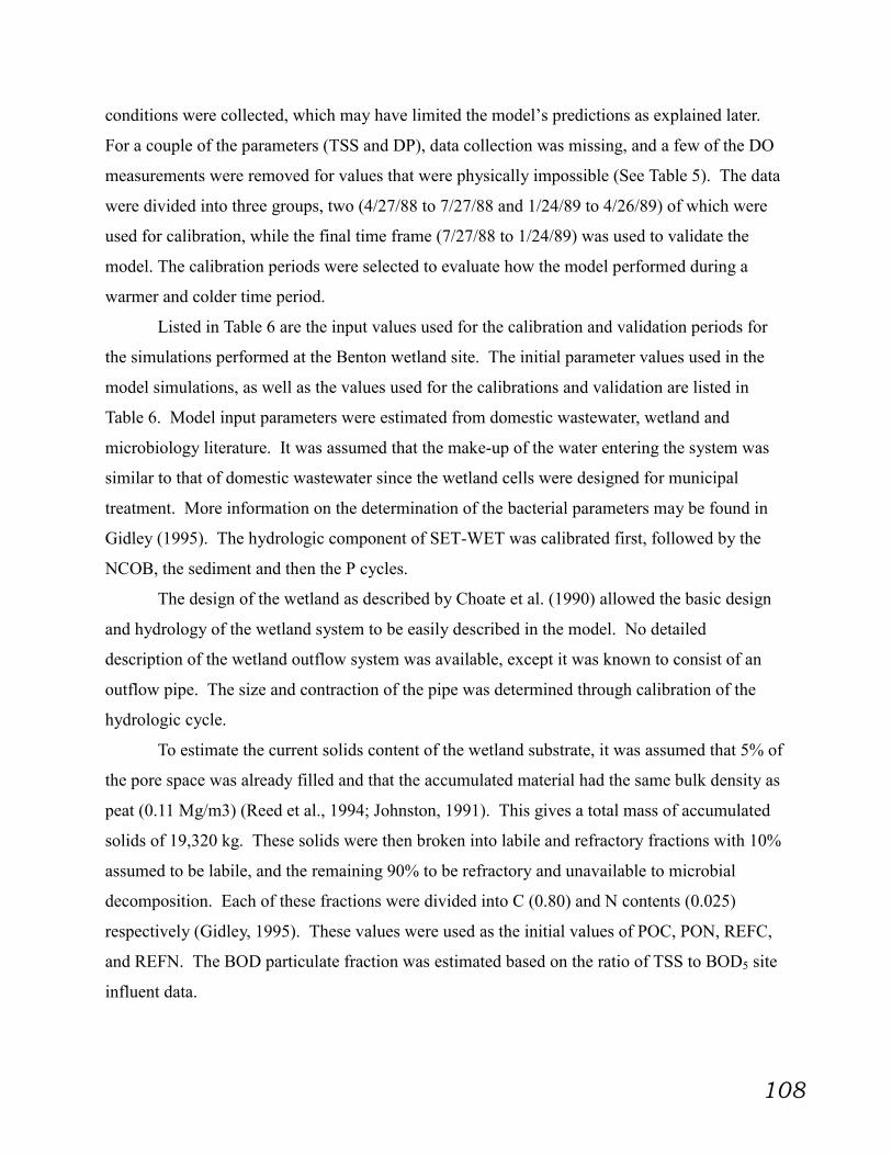
108

conditions were collected, which may have limited the model’s predictions as explained later.

For a couple of the parameters (TSS and DP), data collection was missing, and a few of the DO

measurements were removed for values that were physically impossible (See Table 5). The data

were divided into three groups, two (4/27/88 to 7/27/88 and 1/24/89 to 4/26/89) of which were

used for calibration, while the final time frame (7/27/88 to 1/24/89) was used to validate the

model. The calibration periods were selected to evaluate how the model performed during a

warmer and colder time period.

Listed in Table 6 are the input values used for the calibration and validation periods for

the simulations performed at the Benton wetland site. The initial parameter values used in the

model simulations, as well as the values used for the calibrations and validation are listed in

Table 6. Model input parameters were estimated from domestic wastewater, wetland and

microbiology literature. It was assumed that the make-up of the water entering the system was

similar to that of domestic wastewater since the wetland cells were designed for municipal

treatment. More information on the determination of the bacterial parameters may be found in

Gidley (1995). The hydrologic component of SET-WET was calibrated first, followed by the

NCOB, the sediment and then the P cycles.

The design of the wetland as described by Choate et al. (1990) allowed the basic design

and hydrology of the wetland system to be easily described in the model. No detailed

description of the wetland outflow system was available, except it was known to consist of an

outflow pipe. The size and contraction of the pipe was determined through calibration of the

hydrologic cycle.

To estimate the current solids content of the wetland substrate, it was assumed that 5% of

the pore space was already filled and that the accumulated material had the same bulk density as

peat (0.11 Mg/m3) (Reed et al., 1994; Johnston, 1991). This gives a total mass of accumulated

solids of 19,320 kg. These solids were then broken into labile and refractory fractions with 10%

assumed to be labile, and the remaining 90% to be refractory and unavailable to microbial

decomposition. Each of these fractions were divided into C (0.80) and N contents (0.025)

respectively (Gidley, 1995). These values were used as the initial values of POC, PON, REFC,

and REFN. The BOD particulate fraction was estimated based on the ratio of TSS to BOD5 site

influent data.

109

TABLE 6: INPUT PARAMETER VALUES AND SOURCES FOR CALIBRATION AND VALIDATION PERIODS.Initial Value Value Value Typical

Parameter Value 1st. Cal. 2nd Cal. Validation Range Reference

BASELENGTH 333.5 333.5 333.5 333.5 Site Data WIDTH 43.9 43.9 43.9 43.9 Site DataHO 2 2 2 2 Site DataHB 0 0 0 0 Site DataHTI 0.6 0.6 0.6 0.6 Site DataHII 1.115 1.127 1.01 Site DataSO 0.001 0.001 0.001 0.001 .01-.0001 Reed , 1988

HYDROLOGYPORPEAT 0.3 0.3 0.3 0.3 .2-.4 Brune and Tomasso, 1991

Boyd, 1991OUTLET 3 3 3 3 Site DataHOUT 1.056 1.057 1.056 CalibrationAREAPIPE 0.0105 0.0095 0.01 CalibrationCONTC 0.8 0.9 0.85 CalibrationWATINPUT Site DataPRECIPR NOAA, 1988; NOAA 1989AIRTEMP NOAA, 1988; NOAA 1989DAYLEN .81-1.27 Site Data

BIOMASSBIOINIT 3,800,000 5,000 8,635,000 See discussionSTANDIN 8,000,000 8,000,000 6,000,000 "PEATACRW 300 300 300 300 Johnston, 1991PEATACRB 2,000 2,000 2,000 2,000 Johnston, 1991PEATDENS 110 32 32 32 110 Reed et al., 1994

Johnston, 1991PRATEUP 0.5 0.7 0.7 0.7 CalibrationBIODENS 50 50 50 50 Kadlec and Knight, 1996STDDENS 50 50 50 50 Kadlec and Knight, 1996PBIOUW 0.3 0.4 0.4 0.4 CalibrationPSTDUW 0.3 0.2 0.2 0.2 CalibrationDEGBIO 0.99 0.99 0.99 See discussionDAYSDEG 20 20 20 See discussionBIOMGRR 10 3 3 3 5.-15. Kadlec, 1991

Hammer, 1984

BACTERIANITROSIW 18,300 6,000 1,000 1,000 See discussionNITROSIB 183,000 18,000 2,400 2,400 "HETEROIW 5,300 40,000 10,000 25,000 "HETEROIB 53,000 250,000 230,000 240,000 "NDRATEW/NDRATEB .1 / .1 .002 / .002 .002 / .002 .002 / .002 .05-.15 Henze et al., 1986

Brune and Tommasso, 1991NDOHSATW/NDOHSATB 1. / 1. 1. / 1. 1. / 1. 1. / 1. .4-1.3 Henze et al., 1986

Fritz et al., 1979NMAXGRW/NMAXGRB 1 .005 / .005 .005 / .005 .005 / .005 .3-2.0 Henze et al., 1986NNH4HSCW/NNH4HSCB 1 1 1 1 .2-5.0 Henze et al., 1986

Brune and Tommasso, 1991Grady and Lim, 1980

110

Table 6 (cont.): Input parameter values and sources for calibration and validation periods.Initial Value Value Value Typical

Parameter Value 1st. Cal. 2nd Cal. Validation Range ReferenceAEMAXGRW/AEMAXGRB 6 .05 / .01 .05 / .01 .05 / .01 3.-12. Grady and Lim, 1980ANMAXGRW/ANMAXGRB 4 .05 / .01 .05 / .01 .05 / .01 2.-8. Grady and Lim, 1980HTDRW/HTDRB 0.05 0.001 0.001 0.001 .02-.08 Henze et al., 1986

Brune and Tommasso, 1991Fritz et al., 1979

HTDOHSCW/HTDOHSCB 1 0.5 / 0.5 0.5 / 0.5 0.5 / 0.5 .1-2.0 Henze et al., 1986Strand et al., 1985

HNO3HSCW/HNO3HSCB 0.15 0.15 / 0.15 0.15 / 0.15 0.15 / 0.15 .1-.2 Henze et al., 1986Brune and Tommasso, 1991

HORGHSCW/HORGHSCB 50 50 / 50 50 / 50 50 / 50 15-100 Henze et al., 1986Grady and Lim, 1980Brune and Tommasso, 1991

ANFRACW/ANFRACB .1-.9 .2-.8 .2-.8 .2-.8 0.0-0.4 Henze et al., 1986HTTEMPFW/HTTEMPFB 0.0-1.0 0.0-1.0 0.0-1.0 0.0-1.0 - See discussionWATTEMPW Site DataWATTEMPB Site Data

CARBONREFCINIT 13,900,000 13,900,000 20,000,000 16,000,000 See DiscussionDOCINITW * 30,000 20,000 50,000 "DOCINITB * 40,000 30,000 60,000 "POCINITW * 107,000 75,000 200,000 "POCINITB 1,545,000 2,000,000 3,000,000 2,500,000 "BIOCCONT 0.47 0.47 0.47 0.47 Boyd, 1978BODCFRAC 0.8 0.8 0.8 0.8 StoichiometryBODPFRAC 0.5 0.5 0.5 0.5 StoichiometryLEACHR 0.01 0.01 0.01 Kulshretha and Gopal, 1982

Polunin, 1982MICROBEC 0.53 0.53 0.53 0.53 StoichiometryPEATCC 0.8 0.8 0.8 0.8 Brady, 1984POCFALL 0.7 0.45 0.45 0.45POCRES 0.1 0.001 0.001 0.001 CalibrationMANNC 2 2 2 2RESTHC 0.02 0.01 0.01 0.01 CalibrationPOCSIZE 0.2 0.25 0.15 0.2MTCDOC 0.00005 0.00004 0.00004 0.00004 Cussler, 1997POCCOUT 1 0.75 0.3 0.3 CalibrationBODINFCO Site Data

NITROGENDONINITW * 14,000 5,500 5,000 See DiscussionDONINITB * 14,000 10,000 10,000 "IMMINITW * 50,000 700,000 700,000 "IMMINITB * 2,000,000 7,500,000 9,900,000 "NH4INITW * 27,000 20,250 30,000 "NH4INITB * 20,000 10,000 55,000 "NO3INITW * 2,100 6,000 400 "NO3INITB * 5,000 11,000 4,000 "PONINITW * 16,250 10,000 15,000 " PONINITB 48,000 250,000 100,000 300,000 "REFNINIT 435,000 435,000 565,000 500,000 "BIOMCN 23.5 23.5 23.5 23.5 Boyd, 1978BIOMPN 95 95 95 95 Boyd, 1978HTNO3YW/HTNO3YB 3.29 / 3.29 3.29 / 3.29 3.29 / 3.29 3.29 / 3.29 StoichiometryMICRONC 0.125 0.125 0.125 0.125 Stoichiometry

111

Table 6 (cont.): Input parameter values and sources for calibration and validation periods.Initial Value Value Value Typical

Parameter Value 1st. Cal. 2nd Cal. Validation Range ReferenceNSYIELDW/NSYIELDB 0.3 / 0.3 0.3 / 0.3 0.3 / 0.3 .1-.34 Henze et al., 1986

Tchobangolous and Burton, 1991ONPARTF 0.6 0.6 0.6 Site DataPEATNC 0.025 0.025 0.025 Gidley, 1995PONRES 0.01 0.01 0.01 CalibrationPONFALL 0.25 0.25 0.25MTCDON 0.00002 0.00002 0.00002 Cussler, 1997MTCNH4 0.00006 0.00006 0.00006 Cussler, 1997MTCNO3 0.00006 0.00006 Cussler, 1997PONSIZE 0.05 0.05 0.05RESTHN 0.01 0.01 0.01 CalibrationPONCOUT 0.375 0.375 0.375 CalibrationORGNINC Site DataNH4INC Site DataNO3INC Site Data

DISSOLVED OXYGENDOINITW * 60,000 22,000 15,000 See discussionDOINITB * 15,000 15,000 15,000 "HTDOYW/HTDOYB 0.81 .15 / .15 .15 / .15 .15 / .15 0.81 StoichiometryNSDOYW/NSDOYB 0.084 .02 / .02 .02 / .02 .02 / .02 0.084 StoichiometryDOCONCP 0.001 0.001 0.001MTDOX 0.0001 0.0001 0.0001 Cussler, 1997MTFWSDOC 0.00008 0.00008 0.00008 Cussler, 1997DOXYCSAT 8.5 8.5 8.5 Cussler, 1997BIOOXRB Site DataDOCONCIN Site Data

SEDIMENTSEDCAT 3 2 2 2 See DiscussionSEDRES 1 0.1 0.1 0.1 "SEDSIZE (SEDCLASS) .25-.5 .25-.5 .25-.5 .25-.5 "SEDFALL (SEDCLASS) .3-.8 .3-.7 .3-.6 .3-.7 "

SEDINITW (SEDCLASS) 80,000-300,000

10,000-20,000

10,000-190,000 site data

SEDINITB (SEDCLASS) 1,000,000-23,000,000

12,000,000-28,000,000

1,100,000-26,000,000 site data

SEDSPG (SEDCLASS) 2.65 2.65 2.65 2.65SEDPER (SEDCLASS) 1 1 1 1 Site DataRESTHICK 0.1 0.0015 0.0005 0.001 CalibrationMANNC 2 2.5 2.5 2.5DECOMPR 0.1 0.1 0.1 0.1 CalibrationPSEDDEP 0.5 0.5 0.5 0.5 CalibrationSEDINT . Site Data

PHOSPHOROUSDTPHOSIW 21,000 10,000 38,000 See DiscussionDTPHOSIB 25,000 15,000 40,000 " BTPHOSI 250,000 250,000 250,000 "PPHOSI 10,000 20,000 7,150 "PMINPPC 0.05 0.05 0.05 CalibrationPRMINBPC 0.001 0.0005 0.00075 CalibrationADSORP 2 2 2 Site DataMTCPHOS 0.00006 0.00006 0.00006 Cussler, 1997BIOMPP 300 300 300 Kadlec and Knight, 1996PHOSCON 0 0 0 Site DataDISPHOSC Site DataPPHOSCAL Site Data

112

The initial amount of biomass in the system was determined using the time period (days)

between the start of the growing season and the start of the simulation, multiplied by the

assumed constant growth rate of the system. There were no collected estimates on biomass

amounts in the system, therefore a conservative growth estimate of 3 g/m2-day was assumed

(Kadlec, 1991). The initial amount of standing dead material in the system was similarly

determined using a decay rate of .0126 day –1 multiplied by the length of time between the start

of simulation and the end of the previous growing season (Gidley, 1995).

The initial values of DOC, DON, NH4+, NO3

-, DO, BOD5, DP, TP, and TSS were

determined using the initial water volume and the site effluent concentrations at the start of each

simulation period. The water volume in the system was multiplied by the respective effluent

concentrations to determine the nutrient loads in each system. Since no site data were collected

concerning the concentrations of the nutrients in the wetland substrate, these amounts were

determined through calibration.

The initial amount of heterotroph and autotroph cells in the wetland substrate were

estimated based on values given in Stevenson (1982). NS populations are in the range of 106 –

107 cells/gram of soil. It was assumed that NS were present at a density of 106 cells/gram peat.

Generally there are a larger number of heterotrophs present than autotrophs due to their higher

growth rate, thus a density of 108 heterotroph cells/gram peat was assumed (Stevenson, 1982).

An average cell diameter of 1 µm and a density of 1 g/cm3 were used to determine the mass of

bacteria cells. It was assumed that microbes had roughly the same density as water and that they

were spherical. To convert from the number of cells per soil mass to an estimate of local initial

mass of cells, an average bulk density (1.25 Mg/m3) was used (Brady, 1984). To estimate the

number of bacteria in the wetland surface water it was assumed that the number of bacteria in the

water was 10% of the amount in the substrate. It has been shown that up to 30% of the amount

of bacteria in the substrate, may be located in the surface water (Hatano et al., 1994) for

wastewater constructed wetlands.

There was no site data describing the particle size distribution of the incoming sediment

to the wetland cell; however, since the influent to the wetland system initially passed through one

treatment system, it was assumed that many of the larger particulate particles and aggregates had

113

already settled. Since the breakdown or size of the particles was unknown, only one small

particle category (0.2 mm) was used to describe sediment.

The model was determined to be “calibrated” through visual analysis of the graphical

output (Figures 24a to 32b) of the predicted and observed values for the hydrology and nutrients.

Since SET-WET models the interactions between various nutrient cycles, it can be difficult to

simultaneously calibrate all of the cycles. This is because a parameter change for one cycle can

affect up to eight other cycles. For example, the rate of mineralization will affect the amount of

organic N and NH4+ in the system. In addition, this rate will affect the ratio of TON to TOC in

the system, which in combination with the MICTCN ratio determines if the system is N or C

limited. These effects will be further explored with the sensitivity analysis.

Table 7 lists the differences between the observed and predicted values for the Benton

site. The data shows that the predicted values of SET-WET mostly follows the trends for the two

calibration periods. From visual analysis, the hydrology (Figures 24a and 24b), BOD5 (Figures

29a and 29b), dissolved P (Figures 31a and 31b), and total P (Figures 32a and 32b) predictions

values followed the observed values trends the best.

Ammonium concentrations were over-predicted for the first calibration period, while the

NO3-, organic N, and DO effluent concentration predictions did not completely match the trends

for the observed values. The objective of the calibration process was to examine the effects of

both warmer and colder seasons in the study area. Since there were limited data for each

calibration period (4 data points each), each calibration period was modeled as one season

period, eliminating the ability to change parameter values during the simulation. The high NH4+

predictions may be attributable to the extremely high influent concentrations on April 27, 1988

and May 25, 1988 for the Benton wetlands. These two data points were averaged over the entire

time period, meaning for a one-month period, the model was receiving input concentrations of 12

mg/L for NH3-N. These measurements may have been spikes in the observed measurements,

which would contribute to the high NH4+ predictions by the model. Any errors in the input

measurements will be amplified for all nutrients because so few data points were available.

For the second calibration period (1/24/88 to 4/26/89), the DO concentration predictions

were over predicted. Once again this can probably be attributed to the lack of sufficient data

points used for input. The measured incoming DO counts, for the entire second calibration

period were at high levels. Another reason DO values may have been over-predicted is due to

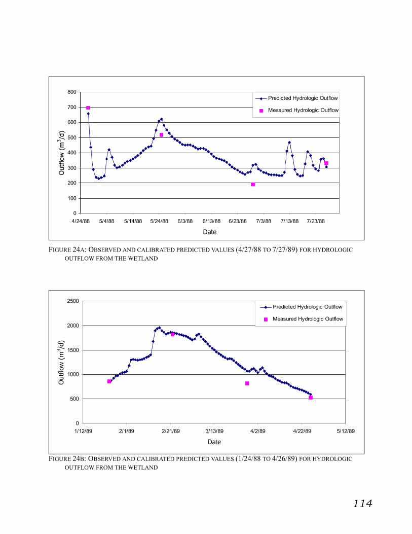
114

0

100

200

300

400

500

600

700

800

4/24/88 5/4/88 5/14/88 5/24/88 6/3/88 6/13/88 6/23/88 7/3/88 7/13/88 7/23/88

Date

Out

flow

(m

3 /d)

Predicted Hydrologic Outflow

Measured Hydrologic Outflow

FIGURE 24A: OBSERVED AND CALIBRATED PREDICTED VALUES (4/27/88 TO 7/27/89) FOR HYDROLOGIC

OUTFLOW FROM THE WETLAND

0

500

1000

1500

2000

2500

1/12/89 2/1/89 2/21/89 3/13/89 4/2/89 4/22/89 5/12/89

Date

Out

flow

(m

3 /d)



FIGURE 24B: OBSERVED AND CALIBRATED PREDICTED VALUES (1/24/88 TO 4/26/89) FOR HYDROLOGIC


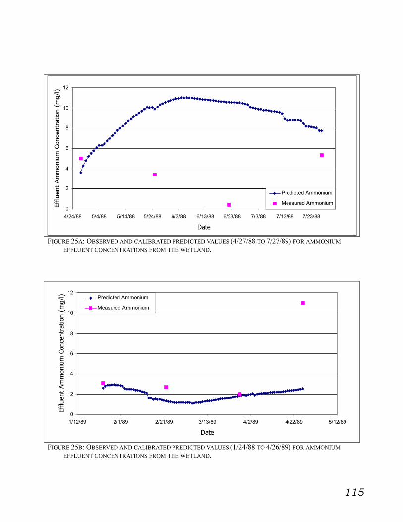
115

0

2

4

6

8

10

12

4/24/88 5/4/88 5/14/88 5/24/88 6/3/88 6/13/88 6/23/88 7/3/88 7/13/88 7/23/88

Date

Efflu

ent

Amm

oniu

m C

once

ntra

tion

(mg/

l)

Predicted Ammonium

Measured Ammonium

FIGURE 25A: OBSERVED AND CALIBRATED PREDICTED VALUES (4/27/88 TO 7/27/89) FOR AMMONIUM

EFFLUENT CONCENTRATIONS FROM THE WETLAND.

0

2

4

6

8

10

12

1/12/89 2/1/89 2/21/89 3/13/89 4/2/89 4/22/89 5/12/89

Date

Efflu

ent

Amm

oniu

m C

once

ntra

tion

(mg/

l) Predicted Ammonium

Measured Ammonium

FIGURE 25B: OBSERVED AND CALIBRATED PREDICTED VALUES (1/24/88 TO 4/26/89) FOR AMMONIUM


116

0

0.1

0.2

0.3

0.4

0.5

0.6

4/24/88 5/4/88 5/14/88 5/24/88 6/3/88 6/13/88 6/23/88 7/3/88 7/13/88 7/23/88

Date

Efflu

ent

Nitr

ate

Conc

entr

atio

n (m

g/l)

Predicted Nitrate

Measured Nitrate

FIGURE 26A: OBSERVED AND CALIBRATED PREDICTED VALUES (4/27/88 TO 7/27/89) FOR NITRATE


0

0.2

0.4

0.6

0.8

1

1.2

1.4

1/12/89 2/1/89 2/21/89 3/13/89 4/2/89 4/22/89 5/12/89

Date

Efflu

ent

Nitr

ate

Conc

entr

atio

n (m

g/l)

Predicted Nitrate

Measured Nitrate

FIGURE 26B: OBSERVED AND CALIBRATED PREDICTED VALUES (1/24/88 TO 4/26/89) FOR NITRATE


117

0

1

2

3

4

5

4/24/88 5/4/88 5/14/88 5/24/88 6/3/88 6/13/88 6/23/88 7/3/88 7/13/88 7/23/88

Date

Efflu

ent

Org

anic

Nitr

ogen

Conc

entr

atio

n (m

g/l)

Predicted Organic Nitrogen

Measured Organic Nitrogen

FIGURE 27A: OBSERVED AND CALIBRATED PREDICTED VALUES (4/27/88 TO 7/27/89) FOR ORGANIC

NITROGEN EFFLUENT CONCENTRATIONS FROM THE WETLAND.

0

0.5

1

1.5

2

2.5

3

3.5

4

4.5

1/12/89 2/1/89 2/21/89 3/13/89 4/2/89 4/22/89 5/12/89

Date

Efflu

ent

Org

anic

Nitr

ogen

Co

ncen

trat

ion

(mg/

l)



FIGURE 27B: OBSERVED AND CALIBRATED PREDICTED VALUES (1/24/88 TO 4/26/89) FOR ORGANIC


118

0

3

6

9

12

15

4/24/88 5/4/88 5/14/88 5/24/88 6/3/88 6/13/88 6/23/88 7/3/88 7/13/88 7/23/88

Date

Efflu

ent

Dis

solv

ed O

xyge

n Co

ncen

trat

ion

(mg/

l)

Predicted Dissolved Oxygen

Measured Dissolved Oxygen

FIGURE 28A: OBSERVED AND CALIBRATED PREDICTED VALUES (4/27/88 TO 7/27/89) FOR DISSOLVED

OXYGEN EFFLUENT CONCENTRATIONS FROM THE WETLAND.

0

1

2

3

4

5

6

7

8

9

10

1/12/89 2/1/89 2/21/89 3/13/89 4/2/89 4/22/89 5/12/89

Date

Efflu

ent

Dis

solv

ed O

xyge

n Co

ncen

trat

ion

(mg/

l)



FIGURE 28B: OBSERVED AND CALIBRATED PREDICTED VALUES (1/24/88 TO 4/26/89) FOR DISSOLVED


119

0

2

4

6

8

10

12

14

16

18

20

4/24/88 5/4/88 5/14/88 5/24/88 6/3/88 6/13/88 6/23/88 7/3/88 7/13/88 7/23/88

Date

Efflu

ent

BOD

5 Co

ncen

trat

ions

(m

g/l)

Predicted BOD5

Measured BOD5

FIGURE 29A: OBSERVED AND CALIBRATED PREDICTED VALUES (4/27/88 TO 7/27/89) FOR BOD5 EFFLUENT

CONCENTRATIONS FROM THE WETLAND.

0

2

4

6

8

10

12

14

16

18

1/12/89 2/1/89 2/21/89 3/13/89 4/2/89 4/22/89 5/12/89

Date

Efflu

ent

BOD

5 Co

ncen

trat

ions

(m

g/l)

Predicted BOD5

Measured BOD5

FIGURE 29B: OBSERVED AND CALIBRATED PREDICTED VALUES (1/24/88 TO 4/26/89) FOR BOD5 EFFLUENT


120

0

10

20

30

40

50

60

4/24/88 5/4/88 5/14/88 5/24/88 6/3/88 6/13/88 6/23/88 7/3/88 7/13/88 7/23/88

Date

Efflu

ent

Tota

l Sus

pend

ed S

olid

s Co

ncen

trat

ion

(mg/

l)

Predicted TSS

Measured TSS

FIGURE 30A: OBSERVED AND CALIBRATED PREDICTED VALUES (4/27/88 TO 7/27/89) FOR TOTAL

SUSPENDED SOLIDS EFFLUENT CONCENTRATIONS FROM THE WETLAND.

0

5

10

15

20

25

1/12/89 2/1/89 2/21/89 3/13/89 4/2/89 4/22/89 5/12/89

Date

Efflu

ent

Tota

l Sus

pend

ed S

olid

s Co

ncen

trat

ion

(mg/

l)

Predicted TSS

Measured TSS

FIGURE 30B: OBSERVED AND CALIBRATED PREDICTED VALUES (1/24/88 TO 4/26/89) FOR TOTAL

SUSPENDED SOLIDS EFFLUENT CONCENTRATIONS FROM THE WETLAND.

121

0

1

2

3

4

5

6

7

8

9

4/24/88 5/4/88 5/14/88 5/24/88 6/3/88 6/13/88 6/23/88 7/3/88 7/13/88 7/23/88

Date

Efflu

ent

Dis

solv

ed P

hosp

horo

us

Conc

entr

atio

n (m

g/l)

Predicted Dissolved Phosphorous

Measured Dissolved Phosphorous

FIGURE 31A: OBSERVED AND CALIBRATED PREDICTED VALUES (4/27/88 TO 7/27/89) FOR DISSOLVED

PHOSPHOROUS EFFLUENT CONCENTRATIONS FROM THE WETLAND.

0

0.5

1

1.5

2

2.5

3

3.5

4

4.5

1/12/89 2/1/89 2/21/89 3/13/89 4/2/89 4/22/89 5/12/89

Date

Efflu

ent

Dis

solv

ed P

hosp

horo

us

Conc

entr

atio

n (m

g/l)



FIGURE 31B: OBSERVED AND CALIBRATED PREDICTED VALUES (1/24/88 TO 4/26/89) FOR DISSOLVED


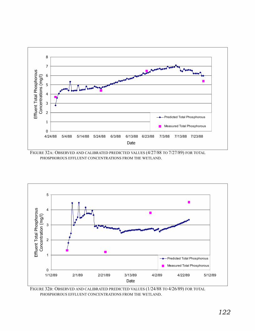
122

0

1

2

3

4

5

6

7

8

4/24/88 5/4/88 5/14/88 5/24/88 6/3/88 6/13/88 6/23/88 7/3/88 7/13/88 7/23/88

Date

Efflu

ent

Tota

l Pho

spho

rous

Co

ncen

trat

ions

(m

g/l)

Predicted Total Phosphorous

Measured Total Phosphorous

FIGURE 32A: OBSERVED AND CALIBRATED PREDICTED VALUES (4/27/88 TO 7/27/89) FOR TOTAL


0

1

2

3

4

5

1/12/89 2/1/89 2/21/89 3/13/89 4/2/89 4/22/89 5/12/89

Date

Efflu

ent

Tota

l Pho

spho

rous

Co

ncen

trat

ion

(mg/

l)



FIGURE 32B: OBSERVED AND CALIBRATED PREDICTED VALUES (1/24/88 TO 4/26/89) FOR TOTAL


123

TABLE 7: MEASURED, PREDICTED, AND DIFFERENCE BETWEEN THE MEASURED AND PREDICTED VALUES

FOR THE HYDROLOGY, AND VARIOUS WETLAND EFFLUENT CONCENTRATIONS FOR THE CALIBRATED,PREDICTED VALUES.

Measured Predicted Difference Measured Predicted

Hydrologic Hydrologic in NH4 NH4

Outflow Outflow Hydrologic Effluent Effluent DifferenceDate (m^3) (m^3) Outflow Conc. (mg/l) Conc. (mg/l) NH4

4/27/88 657.52 696.22 38.70 5 3.58 -1.425/25/88 621.05 518.56 -102.49 3.4 9.92 6.526/29/88 318.32 190.90 -127.42 0.4 10.57 10.177/27/88 305.97 332.33 26.36 5.3 7.72 2.42

1/24/89 864.97 858.29 -6.68 3.1 2.62 -0.482/22/89 1853.03 1815.93 -37.10 2.7 1.36 -1.343/28/89 1071.55 816.99 -254.56 2 1.86 -0.144/26/89 598.78 530.25 -68.53 11 2.54 -8.46

Measured Predicted Measured PredictedNO3 NO3 Organic-N Organic-N

Effluent Effluent Difference Effluent Effluent DifferenceDate Conc. (mg/l) Conc. (mg/l) NO3 Conc. (mg/l) Conc. (mg/l) Organic-N

4/27/88 0.37 0.279 -0.092 3.45 2.67 -0.785/25/88 0.54 0.013 -0.527 4.5 2.96 -1.546/29/88 0.01 0.013 0.003 4.2 3.87 -0.337/27/88 0 0.013 0.013 1.5 4.34 2.84

1/24/89 0.82 0.778 -0.042 1.5 1.20 -0.302/22/89 0.34 0.537 0.197 1 1.74 0.743/28/89 0.15 0.323 0.173 3 2.55 -0.454/26/89 0.01 0.039 0.029 4.2 4.27 0.07

Measured Predicted Measured PredictedDO DO BOD5 BOD5

Effluent Effluent Difference Effluent Effluent DifferenceDate Conc. (mg/l) Conc. (mg/l) DO Conc. (mg/l) Conc. (mg/l) BOD5

4/27/88 8.75 7.10 -1.65 16.50 11.16 -5.345/25/88 11.50 5.01 -6.49 18.00 15.11 -2.896/29/88 0.30 4.13 3.83 6.00 15.04 9.047/27/88 0.20 4.63 4.43 19.00 11.07 -7.93

1/24/89 4.80 5.14 0.34 9.00 4.92 -4.082/22/89 3.80 7.82 4.02 9.00 11.85 2.853/28/89 1.20 5.77 4.57 12.00 12.84 0.844/26/89 0.20 6.48 6.28 16.00 13.33 -2.67

Measured Predicted Measured PredictedTSS TSS Dis.-P Dis.-P

Effluent Effluent Difference Effluent Effluent DifferenceDate Conc. (mg/l) Conc. (mg/l) TSS Conc. (mg/l) Conc. (mg/l) Dis.-P

4/27/88 40.00 39.79 -0.21 3.20 4.61 1.415/25/88 53.00 22.07 -30.93 5.80 6.25 0.456/29/88 23.00 21.36 -1.64 5.40 5.96 0.567/27/88 27.00 21.45 -5.55 3.10 2.79 -0.31

1/24/89 2.00 2.59 0.59 1.40 1.30 -0.102/22/89 2.00 6.14 4.14 1.20 2.83 1.633/28/89 20.00 6.61 -13.39 3.70 2.74 -0.964/26/89 14.00 3.34 -10.66 4.10 3.34 -0.76

124

the estimation of water temperature in the system. Water temperature was estimated from the air

temperature, with the assumption that the water temperature in the surface and substrate water

were the same. These values may have been incorrect, due to the limited data points used in the

regression. In addition, air temperature fluctuates appreciably more than water temperature.

Water temperature is a factor in bacterial growth. If the water temperature is below 0 °C,

bacterial growth will cease, limiting the amount of oxygen consumption in the wetland. There

were no bacterial counts made in the system thus it is unknown if bacteria counts are close to

actual values.

Additionally, matching the predicted and simulated values for sediment was difficult for

the calibration periods. The hydrologic outflow from the system is used to determine the water

velocity in the wetland. The wetland water velocity is then used to determine if resuspension in

the system occurs based on the water velocity being greater than the critical velocity (Equation

32). There is no function controlling the amount of sediment that is lifted up (resuspended) from

the wetland substrate based on the speed above the critical velocity. A set amount is lifted up

whenever the critical velocity is exceeded; this makes the predictions less accurate.

The calibrated values input did not greatly deviate from the values previously

determined through literature, except for parameters directly involving bacterial growth and

oxygen transfer. For the microbial parameters, the most dramatic changes involved the

maximum growth rates, which were changed by two order of magnitudes (from 6.0 and 4.0. to

0.05 and 0.05 for HT bacteria; 1.0 to 0.005 for AT bacteria). The literature values are typical for

conventional wastewater treatment systems, therefore it is not unreasonable for microbial growth

to be slower in a less controlled environment. Additionally, the heterotroph and autotroph yields

and death rates were each decreased significantly. These values would correspond with the

changes associated with the lowering of the growth parameters. If the death parameter were not

lowered to correspond to the decrease in microbial growth parameters, then the bacteria in the

system would completely die out. Furthermore, the microbial yields needed to be changed as the

growth of the microbes is decreased with the smaller growth parameter; therefore, more oxygen

per bacteria is consumed since there is less competition.

125

3. Model Validation:

SET-WET was validated by comparing the model’s predicted results with the observed

data for the period 7/27/88 to 1/24/89. In the validation process, the initial amounts of each

respective nutrient in the system were determined in the same manner as the calibration

procedure, by multiplying the effluent concentrations with the initial water volume in the system.

The input parameter values for the validation period were determined by taking the average of

the two calibration period parameter values (Table 6). On 08/30/88 (16.8 mg/L) and 12/13/88

(19.1 mg/L), the measured DO concentrations were above the maximum DO solubility under

atmospheric conditions (14.62 mg/L at 0 °C; Reed et al., 1994). These values were removed

from the validation process. Figures 33-41 display the model predictions and the observed data

for the outflow and the effluents of NH4+, NO3

-, organic N, DO, BOD5, TSS, DP and TP

concentrations for the validation period. Table 8 lists the measured values, predicted values, and

the difference between the two values for the hydrology outflow, and the NH4+, NO3

-, organic N,

DO, BOD5, TSS, and DP effluent concentrations.

0

200

400

600

800

1000

1200

1400

1600

7/16/88 8/5/88 8/25/88 9/14/88 10/4/88 10/24/88 11/13/88 12/3/88 12/23/88 1/12/89 2/1/89

Date

Out

flow

(m

3 /d)



FIGURE 33: OBSERVED AND VALIDATED PREDICTED VALUES (7/27/88 TO 1/24/89) FOR HYDROLOGIC


126

0

1

2

3

4

5

6

7

8

9

10

7/16/88 8/5/88 8/25/88 9/14/88 10/4/88 10/24/88 11/13/88 12/3/88 12/23/88 1/12/89 2/1/89

Date

Efflu

ent

Amm

oniu

m C

once

ntra

tion

(mg/

l)

Predicted Ammonium

Measured Ammonium

FIGURE 34: OBSERVED AND VALIDATED PREDICTED VALUES (7/27/88 TO 1/24/89) FOR AMMONIUM


0

0.2

0.4

0.6

0.8

1

7/16/88 8/5/88 8/25/88 9/14/88 10/4/88 10/24/88 11/13/88 12/3/88 12/23/88 1/12/89 2/1/89

D a t e

Efflu

ent

Nitr

ate

conc

entr

atio

n (m

g/l) Predicted Nitrate

Measured Nitrate

FIGURE 35: OBSERVED AND VALIDATED PREDICTED VALUES (7/27/88 TO 1/24/89) FOR NITRATE EFFLUENT


127

0

1

2

3

4

5

6

7

8

7/16/88 8/5/88 8/25/88 9/14/88 10/4/88 10/24/88 11/13/88 12/3/88 12/23/88 1/12/89 2/1/89

Date

Efflu

ent

Org

anic

Nitr

ogen

Con

cent

ratio

n (m

g/l)



FIGURE 36: OBSERVED AND VALIDATED PREDICTED VALUES (7/27/88 TO 1/24/89) FOR ORGANIC


0

1

2

3

4

5

6

7

8

7/16/88 8/5/88 8/25/88 9/14/88 10/4/88 10/24/88 11/13/88 12/3/88 12/23/88 1/12/89 2/1/89

Date

Efflu

ent

Dis

solv

ed O

xyge

n Co

ncen

trat

ion

(mg/

l)



FIGURE 37: OBSERVED AND VALIDATED PREDICTED VALUES (7/27/88 TO 1/24/89) FOR DISSOLVED


128

0

4

8

12

16

20

7/16/88 8/5/88 8/25/88 9/14/88 10/4/88 10/24/88 11/13/88 12/3/88 12/23/88 1/12/89 2/1/89

Date

Efflu

ent

BOD

5 co

ncen

trat

ions

(m

g/l)

Predicted BOD5

Measured BOD5

FIGURE 38: OBSERVED AND VALIDATED PREDICTED VALUES (7/27/88 TO 1/24/89) FOR BOD5 EFFLUENT


0

5

10

15

20

25

30

7/16/88 8/5/88 8/25/88 9/14/88 10/4/88 10/24/88 11/13/88 12/3/88 12/23/88 1/12/89 2/1/89

Date

Efflu

ent

Tota

l Sus

pend

ed S

olid

s Co

ncen

trat

ion

(mg/

l)

Predicted TSS

Measured TSS

FIGURE 39: OBSERVED AND VALIDATED PREDICTED VALUES (7/27/88 TO 1/24/89) FOR TOTAL SUSPENDED

SOLIDS EFFLUENT CONCENTRATIONS FROM THE WETLAND.

129

0

1

2

3

4

5

6

7

8

9

7/16/88 8/5/88 8/25/88 9/14/88 10/4/88 10/24/88 11/13/88 12/3/88 12/23/88 1/12/89 2/1/89

Date

Efflu

ent

Dis

solv

ed P

hosp

horo

us C

once

ntra

tion

(mg/

l)



FIGURE 40: OBSERVED AND VALIDATED PREDICTED VALUES (7/27/88 TO 1/24/89) FOR DISSOLVED


0

1

2

3

4

5

6

7

8

9

10

7/16/88 8/5/88 8/25/88 9/14/88 10/4/88 10/24/88 11/13/88 12/3/88 12/23/88 1/12/89 2/1/89

Date

Efflu

ent

Tota

l Pho

spho

rous

Co

ncen

trat

ion

(mg/

l)



FIGURE 41: OBSERVED AND VALIDATED PREDICTED VALUES (7/27/88 TO 1/24/89) FOR TOTAL


130

TABLE 8: MEASURED, PREDICTED, AND DIFFERENCE BETWEEN THE MEASURED AND PREDICTED VALUES

FOR THE HYDROLOGY AND VARIOUS WETLAND EFFLUENT CONCENTRATIONS FOR THE VALIDATED,PREDICTED VALUES.

Measured Predicted Difference Measured PredictedHydrologic Hydrologic in NH4 NH4

Outflow Outflow Hydrologic Effluent Effluent DifferenceDate (m^3) (m^3) Outflow Conc. (mg/l) Conc. (mg/l) NH4

7/27/88 332.33 345.64 -13.31 5.30 4.36 0.948/30/88 473.75 424.41 49.34 8.60 3.54 5.069/28/88 332.33 371.21 -38.88 8.40 2.83 5.5710/25/88 560.24 492.28 67.96 9.00 6.22 2.7811/29/88 1355.81 1274.87 80.94 4.60 5.53 -0.9312/13/88 864.91 631.60 233.31 3.80 5.02 -1.221/24/89 858.29 856.48 1.81 3.10 4.99 -1.89

Measured Predicted Measured PredictedNO3 NO3 Organic-N Organic-N

Effluent Effluent Difference Effluent Effluent DifferenceDate Conc. (mg/l) Conc. (mg/l) NO3 Conc. (mg/l) Conc. (mg/l) Organic-N

7/27/88 0.01 0.06 -0.05 1.50 1.54 -0.048/30/88 0.01 0.01 0.00 4.90 4.28 0.629/28/88 0.02 0.00 0.02 7.20 3.95 3.2510/25/88 0.17 0.03 0.14 2.40 3.26 -0.8611/29/88 0.55 0.54 0.01 1.00 2.85 -1.8512/13/88 0.76 0.54 0.22 2.40 2.77 -0.371/24/89 0.82 0.46 0.36 1.50 1.22 0.28

Measured Predicted Measured PredictedDO DO BOD5 BOD5

Effluent Effluent Difference Effluent Effluent DifferenceDate Conc. (mg/l) Conc. (mg/l) DO Conc. (mg/l) Conc. (mg/l) BOD5

7/27/88 0.20 3.94 -3.74 19.00 14.28 4.738/30/88 1.40 7.83 -6.43 11.00 11.85 -0.859/28/88 3.60 5.04 -1.44 9.00 9.24 -0.2410/25/88 2.50 5.62 -3.12 5.00 9.48 -4.4811/29/88 4.00 6.59 -2.59 8.00 11.78 -3.7812/13/88 3.30 9.34 -6.04 7.00 15.62 -8.621/24/89 4.80 7.42 -2.62 9.00 14.19 -5.19

Measured Predicted Measured PredictedTSS TSS Dis.-P Dis.-P

Effluent Effluent Difference Effluent Effluent DifferenceDate Conc. (mg/l) Conc. (mg/l) TSS Conc. (mg/l) Conc. (mg/l) Dis.-P

7/27/88 27.00 27.62 -0.62 5.40 5.52 -0.128/30/88 11.00 2.47 8.53 5.30 6.36 -1.069/28/88 9.00 2.53 6.47 5.80 5.62 0.1810/25/88 2.00 2.60 -0.60 4.30 4.59 -0.2911/29/88 4.00 4.15 -0.15 2.80 2.56 0.2412/13/88 3.00 3.89 -0.89 2.80 2.64 0.161/24/89 2.00 3.34 -1.34 1.40 1.24 0.16

131

The data set used to calibrate and validate the SET-WET model was not ideal, as the use

of monthly linear interpolation between the observed data points contradicts the principle idea of

NPS pollution’s randomness and dependence upon climatic occurrences. Since the Benton

wetland site is developed for municipal waste treatment, however, this problem may have been

mitigated. The ideal data set would consist of daily data points for all concerned hydrologic and

nutrient parameters over a minimum of two-years, but no such data were available. This type of

data set would allow the seasonal as well as long term comparison of model performances.

As evident in Figures 33-41, the predicted trends for the validated period match the

observed values fairly well for various parameters, except for the NH4+ (Figure 34) and DO

(Figure 37) predictions. The trend for predicted NH4+ concentrations does not follow the

measured values for the period of middle of August 1988 to the end of October 1988. During

this period, the model’s predictions are low, thus implying that the conversion of organic N

through mineralization is not sufficiently handled by the model for this period. However when

one examines the organic N concentration (Figure 36), there is not an overestimation of values;

therefore, the model may be under-predicting organic N amounts due to a lack of accounting for

biomass degradation and possible additions from N fixation. Another possible explanation for

the extremely low NH4+ predictions is the very low influent NH4

+ concentrations during this time

frame. The values are comparably low and as stated earlier, since the data points are so few, any

major errors in measurements during data collection will have a significant effect on model

input.

The inability of the model to match DO concentrations is a cause for concern. This

concern stems from the fact that many of the bacterial growth and bacteria uptake rates are

directly and indirectly affected by oxygen concentrations in the system. It is possible that the

assumption of a constant oxygen transfer rate by plants during the growing season may be

incorrect, as the DO concentrations are much higher than observed.

The dissolved concentrations associated with the total P effluent (Figures 40 and 41)

comprise a significant percentage of the total P. These values suggest that there is a significant

amount of particulate P buried in the system, which is in accordance with findings of previous

researchers (Kadlec and Knight, 1996).

To confirm that the model is performing proper mathematical calculations, a mass

balance of various hydrologic and nutrient pools of the model’s predictions were performed.

132

The cumulative inflows and outflows from the system were determined for every pool in the

system. The difference between these two values was compared with the change in storage in

the system, which is the difference between the final and initial amounts for each pool. The

largest percent difference between these values was 1%, indicating that the model sufficiently

accounted for the interactions of each pool.

From visual analysis of the data points it appears that the data matches very well

considering the data limitations. Further support will be lent by the statistical analyses.

B. Statistical Analysis:

Statistical analyses were performed on the differences between the observed

measurements and model’s predicted values for the hydrology, and nutrient parameters. The

SAS software package “proc univariate’ procedure was used to perform the Wilcoxon signed

rank test on the data (Ott, 1993). In the test, the null hypothesis (H0) was that there are no

differences between the observed and predicted values, while the alternative hypotheses (H1) is

that there are significant differences between the values. Using a two-sided test, with an alpha

value of 0.10, it was determined whether the model predictions were similar to the measured

values.

Ordinarily, the objective of a statistical test is to try to reject the null hypothesis, giving

fairly strong support to the alternative hypothesis. The Wilcoxon test is not designed in this

manner, therefore, we do not want to reject the null hypothesis. Failure to reject the hypothesis

means acceptance of H0, indicating that the observed and predicted values are not statistically

different from each other. A p-value that is greater than the alpha cut-off value of 0.10 would

result in the failure to reject the null hypothesis. The confidence level in this comparison

increases as the reported p-value approaches the maximum value of 1.0.

Table 9 presents the p-values for the differences between the observed measurements and

predicted model values for selected outflow parameters. For the hydrology, NO3-, NH4

+, organic

N, BOD5, TSS, dissolved and total P outflows, we failed to reject the null hypothesis, as their p-

values are greater than 0.10 indicating that the measured and predicted values were statistically

similar. The only parameter for which the null hypothesis was rejected was DO, whose p-value

was 0.016. These results must be examined closely however, as there were only seven values

133

TABLE 9: P-VALUES AND RESULTS OF THE WILCOXON SIGNED RANK TEST PROCEDURE FOR DIFFERENCES

BETWEEN THE MEASURED AND VALIDATED, PREDICTED VALUES OF WETLAND EFFLUENT IN BENTON,KENTUCKY.

Outflow Parameter P-value H0

Hydrology 0.156 AcceptNitrate 0.375 Accept

Ammonium 0.297 AcceptOrganic Nitrogen 0.938 Accept

Dissolved Oxygen 0.016 Not AcceptBOD 5 0.109 Accept

Total Suspended Solids 0.938 AcceptDissolved Phosphorous 0.999 Accept

Total Phosphorous 0.688 Accept

in the data set used for each comparison. The Wilcoxon signed rank test is more reliable when

more observations are used. For the BOD5 (p=0.109), and hydrology (p=0.156) comparisons,

the p-values are barely above the cutoff value, meaning that caution should be used in failing to

reject the null hypothesis. On the other hand, the p-values for the TSS (p=0.938), ON (p=.0938),

and DP (p=0.999) are close to one, indicating a higher confidence in the acceptance of the null

hypothesis because the values are symmetrical around the observed values. Results of the

statistical analyses indicate that the SET-WET model predicted values that are similar to the

observed data.

In addition to the Wilcoxon signed rank test, linear regression was also performed on the

output values. The regression analysis was used to compare the measured and predicted values

for the nutrients and hydrology of the wetland. For this analysis, our null hypothesis (H0) was

that the slope coefficient between the observed and predicted values is zero, while the alternative

hypothesis (H1) was that the slope coefficient is not equal to zero. The ideal situation, which is

referred to as the 1:1 line, would be a line that crosses the y intercept (B0) at zero and has a slope

(B1) of one. This line represents the situation in which the observed and predicted values are

exactly the same.

Table 10 lists the results of the linear regression analysis. The values for B0 and B1 are the

linear regression of the simulated (independent variable) and observed (dependent variable) data

points, respectively. Because SET-WET is a deterministic model, the simulated values are used

as the independent values since the model will always predict these values with the same data

input. There is variability and uncertainty in the observed values since there are differences in

the observed measurements depending on how, when and who takes and analyses the samples

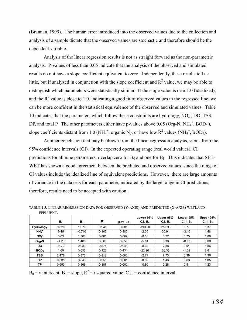
134

(Brannan, 1999). The human error introduced into the observed values due to the collection and

analysis of a sample dictate that the observed values are stochastic and therefore should be the

dependent variable.

Analysis of the linear regression results is not as straight forward as the non-parametric

analysis. P-values of less than 0.05 indicate that the analysis of the observed and simulated

results do not have a slope coefficient equivalent to zero. Independently, these results tell us

little, but if analyzed in conjunction with the slope coefficient and R2 value, we may be able to

distinguish which parameters were statistically similar. If the slope value is near 1.0 (idealized),

and the R2 value is close to 1.0, indicating a good fit of observed values to the regressed line, we

can be more confident in the statistical equivalence of the observed and simulated values. Table

10 indicates that the parameters which follow these constraints are hydrology, NO3-, DO, TSS,

DP, and total P. The other parameters either have p-values above 0.05 (Org-N, NH4+, BOD5 ),

slope coefficients distant from 1.0 (NH4+, organic N), or have low R2 values (NH4

+, BOD5).

Another conclusion that may be drawn from the linear regression analysis, stems from the

95% confidence intervals (CI). In the expected operating range (real world values), CI

predictions for all nine parameters, overlap zero for B0 and one for B1. This indicates that SET-

WET has shown a good agreement between the predicted and observed values, since the range of

CI values include the idealized line of equivalent predictions. However, there are large amounts

of variance in the data sets for each parameter, indicated by the large range in CI predictions;

therefore, results need to be accepted with caution.

TABLE 10: LINEAR REGRESSION DATA FOR OBSERVED (Y-AXIS) AND PREDICTED (X-AXIS) WETLAND

EFFLUENT.Lower 95% Upper 95% Lower 95% Upper 95%

B0 B1 R2p-value C.I. B0 C.I. B0 C. I. B1 C. I. B1

Hydrology 9.820 1.070 0.945 0.001 -199.30 218.93 0.77 1.37

NH4+ 9.45 -0.710 0.105 0.480 -2.05 20.94 -3.10 1.68

NO3- 0.03 1.300 0.881 0.002 -0.16 0.22 0.75 1.86

Org-N -1.23 1.480 0.560 0.053 -5.81 3.36 -0.03 3.00

DO -2.72 0.933 0.574 0.048 -8.32 2.88 0.01 1.86

BOD5 1.69 0.650 0.126 0.434 -22.96 26.35 -1.32 2.61

TSS 2.478 0.873 0.812 0.006 -2.77 7.73 0.39 1.36

DP 0.535 0.843 0.956 0.001 -0.39 1.46 0.63 1.05

TP 0.693 0.869 0.887 0.002 -0.90 2.28 0.51 1.23

B0 = y intercept, B1 = slope, R2 = r squared value, C.I. = confidence interval

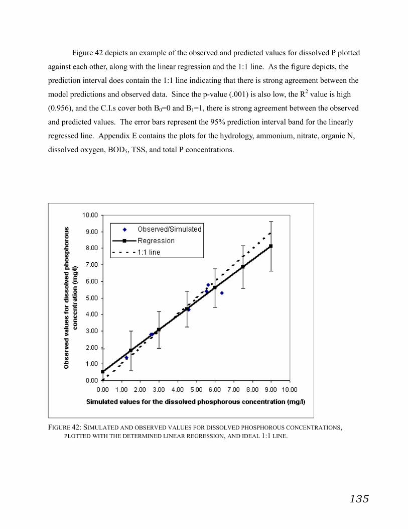
135

Figure 42 depicts an example of the observed and predicted values for dissolved P plotted

against each other, along with the linear regression and the 1:1 line. As the figure depicts, the

prediction interval does contain the 1:1 line indicating that there is strong agreement between the

model predictions and observed data. Since the p-value (.001) is also low, the R2 value is high

(0.956), and the C.I.s cover both B0=0 and B1=1, there is strong agreement between the observed

and predicted values. The error bars represent the 95% prediction interval band for the linearly

regressed line. Appendix E contains the plots for the hydrology, ammonium, nitrate, organic N,

dissolved oxygen, BOD5, TSS, and total P concentrations.

FIGURE 42: SIMULATED AND OBSERVED VALUES FOR DISSOLVED PHOSPHOROUS CONCENTRATIONS,PLOTTED WITH THE DETERMINED LINEAR REGRESSION, AND IDEAL 1:1 LINE.

136

C. Sensitivity Analysis:

A sensitivity analysis was conducted to determine which parameters would require the

most scrutiny in future simulations. The relative sensitivity (RS) of each parameter was

determined with the following equation (Heatwole, 1998):

−−

=b

b

b

bR O

P

PP

OOS * (85)

where SR is the relative sensitivity; O is the model output variable of interest; P is the parameter

value; and b is a subscript which represents the parameter values and output of the base scenario.

Each examined parameter was adjusted a total of six times, with changes of (+/-) 10%,

(+/-) 25%, and (+/-) 50%. The cumulative average value for the base scenario was compared

with the average change in model response for the hydrologic and nutrient components. If the

absolute value of the unitless RS is equal to one, then the same percent change occurs in the

output and input; if the RS is less then one, the model response is damped; while an RS value

greater than one indicates the model response is inflated. If the RS value is equal to zero, then

the selected parameter has no effect on the outcome of the component’s predicted values.

Additionally, if the RS value is positive or negative, it can be determined if there is an indirect (-)

or direct (+) relationship between the parameter and the output (Heatwole, 1998).

Table 11 presents the relative sensitivity analysis results for changes of (+/-) 50% to the

base value. Appendix F contains the tables for the relative sensitivity changes of (+/-) 10% and

(+/-) 25%. The data is presented for the hydrologic and nutrient components of SET-WET. The

results of the (+) 50% change are presented first followed by the results of the (–) 50% change.

The (+/-) sign designates whether the RS value relation is direct or indirect, while the letters

represent the one of seven categories into which the RS value falls. A note is made of the ‘NC’

category, which indicates that the simulation run was incomplete due to the generation of

unintelligible results. Parameter values could not be changed (+) 50% for certain situations in

which the parameters were fractions. A (+) 50% change resulted in a fractional value greater

than one, which is impossible. For these cases (PEATCC, BODCFRAC, and PONCOUT), Table

11 presents RS values for a change of +25% from the base. For SET-WET, the results of the

137

TABLE 11: SENSITIVITY ANALYSIS RESULTS OF SET-WET MODEL AS APPLIED TO THE BENTON WETLAND FOR (+/-) 50% CHANGE IN BASE VALUESP a r a m e te r B a s e V a lu e N H 4 N O 3 D O N P O N D O B O D 5 T S S D P T PB A C T E R I A

A E M A X G R B 0 . 0 1 (N C )/ (+ E ) (N C )/ (-D ) (N C )/ (-C ) (N C )/ (-C ) (N C )/ (-E ) (N C )/ (-C ) A / A A / (-C ) (A / -C )A E M A X G R W 0 . 0 5 (+ E )/ (+ D ) (-C )/ (-C ) (-D )/ (-C ) (-C )/ (-C ) (-D )/ (-D ) (-D )/ (-C ) A / A A / A A / AA N M A X G R B 0 . 0 1 (+ D )/ (+ D ) (-D )/ (-D ) (-B )/ (-B ) (-B )/ (-B ) (-C )/ (-C ) (-B )/ (-B ) A / A A / A A / AA N M A X G R W 0 . 0 5 (+ B )/ (+ B ) (-C )/ (-C ) (-B )/ (-B ) (-B )/ (-B ) (-B )/ (-B ) (-B )/ (-B ) A / A A / A A / A

H E T R O I B 2 4 0 0 0 0 (N C )/ (+ E ) (N C )/ (-E ) (N C )/ (-C ) (N C )/ (-C ) (N C )/ (-E ) (N C )/ (-C ) A / A A / A A / AH E T E R O I W 2 5 0 0 0 (+ D )/ (+ D ) (-C )/ (-C ) (-C )/ (-C ) (-B )/ (-B ) (-D )/ (-D ) (-C )/ (-C ) A / A A / A A / AH N O 3 H S C B 0 . 1 5 (-C )/ (-D ) (+ D )/ (+ D ) (+ B )/ (+ B ) (+ B )/ (+ B ) (+ B )/ (+ B ) (+ B ) A / A A / A A / AH N O 3 H S C W 0 . 1 5 (-B )/ (-B ) (+ B )/ (+ B ) (+ B )/ (+ B ) (+ B )/ (+ B ) (+ B )/ (+ B ) (+ B )/ (+ B ) A / A A / A A / AH O R G H S C B 5 0 (-C )/ (-D ) (+ C )/ (+ C ) (+ B )/ (+ B ) (+ B )/ (+ B ) (+ C )/ (+ C ) (+ B )/ (+ B ) A / A A / A A / AH O R G H S C W 5 0 (-C )/ (N C ) (+ C )/ (N C ) (+ C )/ (N C ) (+ B )/ (N C ) (+ D )/ (N C ) (+ C )/ (N C ) A / A A / A A / AH T D O H S C B 0 . 1 5 (-D )/ (N C ) (-C )/ (N C ) (+ C )/ (N C ) (+ C )/ (N C ) (+ D )/ (N C ) (+ C )/ (N C ) A / A A / A A / AH T D O H S C W 0 . 5 (-C )/ (-C ) (-C )/ (-C ) (+ B )/ (+ B ) (+ B )/ (+ B ) (+ C )/ (+ C ) (+ B )/ (+ B ) A / A A / A A / A

H T D R B 0 . 0 0 1 2 5 (-D )/ (-E ) (+ D )/ (+ D ) (+ B )/ (+ C ) (+ B )/ (+ C ) (+ D )/ (+ D ) (+ B )/ (+ C ) A / A A / A A / AH T D R W 0 . 0 0 1 (-C )/ (-C ) (+ B )/ (+ B ) (+ B )/ (+ B ) (+ C )/ (+ C ) (+ C )/ (+ C ) (+ B )/ (+ B ) A / A A / A A / A

N D O H S A T B 1 (-C )/ (-C ) (-C )/ (-C ) (+ B )/ (+ B ) (+ B )/ (+ B ) (+ C )/ (+ C ) (+ B )/ (+ B ) A / A A / A A / AN D O H S A T W 1 (-B )/ (-B ) (-C )/ (-C ) (+ B )/ (+ B ) (+ B )/ (+ B ) (+ C )/ (+ C ) (+ B )/ (+ B ) A / A A / A A / A

N D R A T E B 0 . 0 0 2 (-C )/ (-C ) (-C )/ (-C ) (+ B )/ (+ B ) (+ B )/ (+ B ) (+ C )/ (+ C ) (+ B )/ (+ B ) A / A A / A A / AN D R A T E W 0 . 0 0 2 (-B )/ (-B ) (-C )/ (-C ) (-B )/ (-B ) (-B )/ (-B ) (+ C )/ (+ B ) (-B )/ (-B ) A / A A / A A / AN I T R O S I B 2 4 0 0 (+ D )/ (+ D ) (+ D )/ (+ D ) (-B )/ (-B ) (-C )/ (-B ) (-D )/ (-D ) (-B )/ (-B ) A / A A / A A / AN I T R O S I W 1 0 0 0 (+ C )/ (+ C ) (+ D )/ (+ D ) (-B )/ (-B ) (-B )/ (-B ) (-C )/ (-C ) (-B )/ (-B ) A / A A / A A / AN M A X G R B 0 . 0 0 5 (-D )/ (N C ) (-F )/ (N C ) (+ E )/ (N C ) (-D )/ (N C ) (+ D )/ (N C ) (-E )/ (N C ) A / A A / A A / AN M A X G R W 0 . 0 0 5 (+ C )/ (+ C ) (+ D )/ (+ D ) (-B )/ (-B ) (-B )/ (-B ) (-D )/ (-D ) (-B )/ (-B ) A / A A / A A / AN N H 4 H S C B 1 (-C )/ (-C ) (-C )/ (-C ) (+ B )/ (+ B ) (+ B )/ (+ B ) (+ C )/ (+ (C ) (+ B )/ (+ B ) A / A A / A A / AN N H 4 H S C W 1 (-B )/ (-B ) (-C )/ (-C ) (+ B )/ (+ B ) (+ B )/ (+ B ) (+ C )/ (+ C ) (+ B )/ (+ B ) A / A (-C )/ (+ C ) (-C )/ (+ C )

N I T R O G E NB I O M C N 2 3 .5 (+ D )/ (-D ) (+ F )/ (-B ) (-C )/ (-C ) (-D )/ (-E ) (-C )/ + B ) (-B )/ (+ B ) (-B )/ (+ B ) (-B )/ (+ B ) (-B )/ (+ B )B I O M P N 9 5 (+ E )/ (+ E ) (+ D )/ (+ D ) (-B )/ (-B ) (-C )/ (+ C ) (-C )/ (-D ) (-B )/ (-B ) (-B )/ (+ B ) (-B )/ (+ B ) (-B )/ (+ B )

D O N I N I T B 1 0 0 0 0 (+ B )/ (+ C ) (-B )/ (+ B ) (+ D )/ (+ D ) (-C )/ (+ C ) (-B )/ (-B ) (-B )/ (+ B ) (-B )/ (+ B ) (-B )/ (+ B ) (-B )/ (+ B )D O N I N I T W 5 0 0 0 (-B )/ (+ C ) (-B )/ (+ B ) (+ D )/ (+ D ) (-C )/ (+ C ) (-B )/ (-B ) (-B )/ (+ B ) (-B )/ (+ B ) (-B )/ (+ B ) (-B )/ (+ B )H T N O 3 Y B 3 . 2 9 (+ C )/ (+ D ) (+ D )/ (+ D ) (-B )/ (-B ) (-C )/ (+ C ) (-B )/ (-B ) (-B )/ (-B ) (-B )/ (+ B ) (-B )/ (+ B ) (-B )/ (+ B )H T N O 3 Y W 3 . 2 9 (-B )/ (+ B ) (+ C )/ (+ C ) (-B )/ (+ B ) (-C )/ (+ C ) (-B )/ (-B ) (-B )/ (+ B ) (-B )/ (+ B ) (-B )/ (+ B ) (-B )/ (+ B )I M M IN I T B 9 9 0 0 0 0 0 (-B )/ (+ C ) (-B )/ (+ B ) (-B )/ (+ B ) (-C )/ (+ D ) (-B )/ (-B ) (-B )/ (+ B ) (-B )/ (+ B ) (-B )/ (+ B ) (-B )/ (+ B )I M M IN I T W 7 0 0 0 0 0 (-B )/ (+ B ) (-B )/ (+ B ) (-B )/ (+ B ) (-C )/ (+ C ) (-B )/ (+ B ) (-B )/ (+ B ) (-B )/ (+ B ) (-B )/ (+ B ) (-B )/ (+ B )M I C R O N C 0 . 1 2 5 (-C )/ (-D ) (-B )/ (-B ) (-B )/ (+ B ) (+ D )/ (+ D ) (+ B )/ (+ B ) (-B )/ (+ B ) (-B )/ (+ B ) (-B )/ (+ B ) (-B )/ (+ B )M T C D O N 0 . 0 0 0 0 2 (-B )/ (+ B ) (-B )/ (+ B ) (+ C )/ (+ C ) (-C )/ (+ C ) (-B )/ (+ B ) (-B )/ (+ B ) (-B )/ (+ B ) (-B )/ (+ B ) (-B )/ (+ B )M T C N H 4 0 . 0 0 0 0 6 (-C )/ (-C ) (-B )/ (-B ) (-B )/ (-B ) (-C )/ (+ C ) (-B )/ (-B ) (-B )/ (+ B ) (-B )/ (+ B ) (-B )/ (+ B ) (-B )/ (+ B )M T C N O 3 0 . 0 0 0 0 6 (+ C )/ (+ C ) (+ C )/ (+ D ) (-B )/ (-B ) (-C )/ (+ C ) (-B )/ (-B ) (-B )/ (-B ) (-B )/ (+ B ) (-B )/ (+ B ) (-B )/ (+ B )N H 4 IN I T B 5 5 0 0 0 (+ E )/ (+ E ) (+ C )/ (+ C ) (-B )/ (-B ) (-C )/ (+ C ) (-C )/ (-C ) (-B )/ (-B ) (-B )/ (+ B ) (-B )/ (+ B ) (-B )/ (+ B )N H 4 IN I T W 3 0 0 0 0 (+ D )/ (+ D ) (+ B )/ (+ C ) (-B )/ (-B ) (-C )/ (+ C ) (-C )/ (-C ) (-B )/ (-B ) (-B )/ (+ B ) (-B )/ (+ B ) (-B )/ (+ B )N O 3 IN I T B 4 0 0 0 (+ C )/ (-D ) (+ D )/ (-F ) (-B )/ (+ C ) (-C )/ (+ C ) (-B )/ (+ C ) (-B )/ (-+ B ) (-B )/ (+ B ) (-B )/ (+ B ) (-B )/ (+ B )

138

TABLE 11 (CONT.) SENSITIVITY ANALYSIS RESULTS OF SET-WET MODEL AS APPLIED TO THE BENTON WETLAND FOR (+/-)50% CHANGE IN BASE VALUES

P a r a m e te r B a s e V a lu e N H 4 N O 3 D O N P O N D O B O D 5 T S S D P T PN S Y IE L D B 0 . 3 (-B )/ (+ C ) (-D )/ (-D ) (+ B )/ (+ B ) (-C )/ (+ C ) (+ B )/ (+ B ) (+ B )/ (+ B ) (-B )/ (+ B ) (-B )/ (+ B ) (-B )/ (+ B )N S Y IE L D W 0 . 3 (-C )/ (+ C ) (-D )/ (-D ) (+ B )/ (+ B ) (-C )/ (+ C ) (+ B )/ (+ B ) (-B )/ (+ B ) (-B )/ (+ B ) (-B )/ (+ B ) (-B )/ (+ B )O N P A R T F 0 . 6 (+ D )/ (+ D ) (+ B )/ (+ B ) (-F )/ (-F ) (+ E )/ (+ E ) (-B )/ (+ B ) (-B )/ (+ B ) (-B )/ (+ B ) (-B )/ (+ B ) (-B )/ (+ B )P O N C O U T 0 . 7 5 (-C )/ (-C ) (-B )/ (-B ) (-B )/ (+ B ) (+ E )/ (+ E ) (+ B )/ (+ B ) (-B )/ (+ B ) (-B )/ (+ B ) (-B )/ (+ B ) (-B )/ (+ B )P O N F A L L 0 . 2 5 (+ C )/ (+ C ) (-B )/ (+ B ) (-B )/ (+ B ) (-E )/ (-F ) (+ B )/ (+ B ) (-B )/ (+ B ) (-B )/ (+ B ) (-B )/ (+ B ) (-B )/ (+ B )P O N I N I T B 3 0 0 0 0 0 (+ E )/ (-D ) (+ F )/ (-F ) (-B )/ (+ B ) (+ C )/ (+ D ) (-C )/ (+ C ) (-B )/ (+ B ) (-B )/ (+ B ) A / A A / AP O N I N I T W 1 5 0 0 0 (+ D )/ (-D ) (+ F )/ (-F ) (-B )/ (+ B ) (+ D )/ (+ D ) (-C )/ (+ C ) (-B )/ (+ B ) (-B )/ (+ B ) (-B )/ (+ B ) (-B )/ (+ B )

P O N R E S 0 . 0 1 (-B )/ (+ B ) (-B )/ (+ B ) (-B )/ (+ B ) (+ D )/ (+ D ) (-B )/ (+ B ) (-B )/ (+ B ) (-B )/ (+ B ) (-B )/ (+ B ) (-B )/ (+ B )P O N S IZ E 0 . 0 5 (-B )/ (+ B ) (-B )/ (+ B ) (-B )/ (+ B ) (-C )/ (+ C ) (-B )/ (+ B ) (-B )/ (+ B ) (-B )/ (+ B ) (-B )/ (+ B ) (-B )/ (+ B )R E F N IN IT 5 0 0 0 0 0 (+ D )/ (-D ) (+ F )/ (-F ) (-B )/ (+ B ) (-C )/ (+ C ) (-C )/ (+ C ) (-B )/ (+ B ) (-B )/ (+ B ) (-B )/ (+ B ) (-B / (+ B )

R E S T H N (N IT ) 0 . 0 1 (-B )/ (+ B ) (-B )/ (+ B ) (-B )/ (+ B ) (+ D )/ (+ D ) (-B )/ (+ B ) (-B )/ (+ B ) (-B )/ (+ B ) (-B / (+ B ) (-B )/ (+ B )

V E G E T A T I O NB I O D E N S 5 0 0 0 (+ B )/ (-B ) A / (-B ) (-B )/ (-B ) (-B )/ (-B ) (-B )/ (-B ) (-B )/ (-B ) (-B )/ (-B ) (-B )/ (-B ) (-B )/ (-B )B I O IN IT 8 6 3 5 0 0 0 (-B )/ (-B ) (-B )/ (-B ) (+ B )/ (+ B ) (+ D )/ (+ D ) (-C )/ (-C ) (+ D )/ (+ D ) (+ B )/ (+ B ) (+ B )/ (+ B ) (+ B )/ (+ B )

P B I O U W 0 . 4 (+ B )/ (+ B ) (+ B )/ (-B ) (+ B )/ (+ B ) (+ B )/ (+ B ) (+ B )/ (+ B ) (+ B )/ (+ B ) (+ B )/ (+ B ) (+ B )/ (+ B ) (+ B )/ (+ B )P E A T A C R B 2 0 0 0 (+ C )/ (+ C ) (+ B )/ (+ B ) (+ B )/ (+ B ) (-B )/ (-B ) (+ B )/ (+ B ) (+ B )/ (+ B ) (-B )/ (-B ) (+ B )/ (+ B ) (+ B )/ (+ B )P E A T A C R W 3 0 0 (+ B )/ (+ B ) (+ B )/ (+ B ) (-B )/ (-B ) (-C )/ (-C ) (+ B )/ (+ B ) (-B )/ (-B ) A / A A / A A / AP E A T D E N S 0 . 7 (-B )/ (-B ) (-B )/ (-B ) (-B )/ (-B ) (-B )/ (-B ) (-B )/ (-B ) (-B )/ (-B ) (+ B )/ (+ C ) (-B )/ (-B ) (-B )/ (-B )P R A T E U P 0 . 7 (-D )/ (+ B ) (+ E )/ (+ D ) (-B )/ (-B ) (-B )/ (-B ) (+ B )/ (+ B ) (-B )/ (-B ) A / A (+ B )/ (+ B ) (+ B )/ (+ B )P S T D U W 0 . 4 (+ B )/ (+ B ) (+ B )/ (+ B ) (+ B )/ (+ B ) (+ B )/ (+ B ) (+ B )/ (+ B ) (+ B )/ (+ B ) (+ B )/ (+ B ) (+ B )/ (+ B ) (+ B )/ (+ B )S T A N D I N 6 0 0 0 0 0 0 (-D )/ (-D ) (-C )/ (-C ) (+ B )/ (+ B ) (+ D )/ (+ D ) (-C )/ (-C ) (+ D )/ (+ D ) (+ B )/ (+ B ) (+ B )/ (+ B ) (+ B )/ (+ B )S T D D E N S 5 0 0 0 (+ B )/ (+ B ) (-B )/ (-B ) (-B )/ (-B ) (-B )/ (-B ) (-B )/ (-B ) (-B )/ (-B ) (-B )/ (-B ) (-B )/ (-B ) (-B )/ (-B )C A R B O N

B I O C C O N T 0 . 4 7 (-D )/ (-D ) (-C )/ (-C ) (+ B )/ (+ B ) (+ D )/ (+ E ) (-C )/ (-C ) (+ D )/ (+ D ) (-B )/ (+ B ) (-B )/ (+ B ) (-B )/ (+ B )B O D C F R A C * 0 . 8 (-C )/ (-C ) (-C )/ (-C ) (+ B )/ (+ B ) (-D )/ (+ C ) (-D )/ (-D ) (-E )/ (-E ) (-B )/ (+ B ) (-B )/ (+ B ) (-B )/ (+ B )B O D P F R A C 0 . 5 (-D )/ (-D ) (+ C )/ (+ C ) (-B )/ (-B ) (-C )/ (+ C ) (+ D )/ (+ C ) (-E )/ (-E ) (-B )/ (+ B ) (-B )/ (+ B ) (-B )/ (+ B )D O C I N I T B 6 0 0 0 0 (-B )/ (+ B ) (-B )/ (-B ) (+ B )/ (+ B ) (-C )/ (+ C ) (-C )/ (-C ) (+ D )/ (+ D ) (-B )/ (+ B ) (-B )/ (+ B ) (-B )/ (+ B )D O C I N I T W 5 0 0 0 0 (-B )/ (+ C ) (-B )/ (-B ) (+ B )/ (+ B ) (-C )/ (+ C ) (-C )/ (-C ) (+ D )/ (+ D ) (-B )/ (+ B ) (-B )/ (+ B ) (-B )/ (+ B )

L E A C H R 0 . 0 1 (-B )/ (+ B ) (-B )/ (+ B ) (+ C )/ (+ C ) (-C )/ (+ C ) (-B )/ (-B ) (+ D )/ (+ C ) (-B )/ (+ B ) (-B )/ (+ B ) (-B )/ (+ B )M I C R O B E C 0 . 5 3 (-B )/ (+ B ) (-B )/ (+ B ) (-B )/ (+ B ) (-C )/ (+ C ) (-B )/ (-B ) (+ B )/ (+ B ) (-B )/ (+ B ) (-B )/ (+ B ) (-B )/ (+ B )

M T C D O C 0 . 0 0 0 0 4 (-B )/ (+ B ) (-B )/ (-B ) (-B )/ (-B ) (-C )/ (+ C ) (-B )/ (-B ) (+ C )/ (+ C ) (-B )/ (+ B ) (-B )/ (+ B ) (-B )/ (+ B )P E A T C C * 0 . 8 (-C )/ (+ B ) (-B )/ (+ B ) (-B )/ (+ B ) (-D )/ (+ C ) (-B )/ (-B ) (+ B )/ (+ B ) (-B )/ (+ B ) (-B )/ (+ B ) (-B )/ (+ B )

P O C C O U T * 0 . 3 (+ B )/ (+ C ) (+ B )/ (+ B ) (-B )/ (-B ) (-C )/ (+ C ) (+ B )/ (+ B ) (+ E )/ (+ E ) (-B )/ (+ B ) (-B )/ (+ B ) (-B )/ (+ B )P O C F A L L 0 . 4 5 (-C )/ (-C ) (+ B )/ (+ C ) (+ B )/ (-B ) (-C )/ (+ C ) (+ B )/ (+ D ) (-E )/ (-E ) (-B )/ (+ B ) (-B )/ (+ B ) (-B )/ (+ B )P O C I N I T B 3 0 0 0 0 0 0 (-D )/ (-D ) (-C )/ (-C ) (+ B )/ (+ C ) (-C )/ (+ D ) (-C )/ (-C ) (+ B )/ (+ C ) (-B )/ (+ B ) (-B )/ (+ B ) (-B )/ (+ B )P O C I N I T W 2 0 0 0 0 0 (-C )/ (-C ) (-B )/ (-B ) (+ B )/ (+ B ) (-C )/ (+ C ) (-C )/ (-C ) (+ C )/ (+ C ) (-B )/ (+ B ) (-B )/ (+ B ) (-B )/ (+ B )

P O C R E S 0 . 0 0 1 (-C )/ (+ B ) (+ B )/ (+ B ) (+ B )/ (+ B ) (-C )/ (+ C ) (+ B )/ (-B ) (-E )/ (-B ) (-B )/ (+ B ) (-B )/ (+ B ) (-B )/ (+ B )P O C S IZ E 0 . 2 (-B )/ (+ B ) (-B )/ (+ B ) (-B )/ (+ B ) (-C )/ (+ C ) (-B )/ (-B ) (-B )/ (+ B ) (-B )/ (+ B ) (-B )/ (+ B ) (-B )/ (+ B )R E F C IN IT 1 5 0 0 0 0 0 0 (+ B )/ (+ B ) (+ B )/ (+ B ) (-B )/ (+ B ) (+ C )/ (+ C ) (-B )/ (+ B ) (-B )/ (+ B ) (-B )/ (+ B ) (-B )/ (+ B ) (-B )/ (+ B )

139

TABLE 11 (CONT.) SENSITIVITY ANALYSIS RESULTS OF SET-WET MODEL AS APPLIED TO THE BENTON WETLAND FOR (+/-)50% CHANGE IN BASE VALUES

P a r a m e t e r B a s e V a lu e N H 4 N O 3 D O N P O N D O B O D 5 T S S D P T PD I S S O L V E D O X Y G E N

D O C O N C P 0 . 0 0 1 (-B ) / (+ B ) ( -B ) / (+ B ) ( -B / (+ B ) ( -C ) / (+ C ) (+ B ) / (+ B ) ( -B ) / (+ B ) ( -B ) / (+ B ) ( -B ) / (+ B ) ( -B ) / (+ B )D O I N I T B 1 5 0 0 0 (-D ) / (-D ) (+ C )/ (+ C ) (+ C )/ (+ C ) ( -C ) / (+ D ) (+ D )/ (+ D ) (+ C )/ (+ C ) ( -B ) / (+ B ) ( -B ) / (+ B ) ( -B ) / (+ B )D O I N I T W 1 5 0 0 0 (-C ) / (-C ) (+ C )/ (+ C ) (+ B ) / (+ C ) ( -C ) / (+ D ) (+ D )/ (+ D ) (+ C )/ (+ C ) ( -B ) / (+ B ) ( -B ) / (+ B ) ( -B ) / (+ B )

D O X Y C S A T 8 . 5 (-E ) / (N C ) (+ D )/ (N C ) (+ C )/ (N C ) ( -C ) / (N C ) (+ E ) / (N C ) (+ C )/ (N C ) ( -B ) / (+ B ) ( -B ) / (+ B ) ( -B ) / (+ B )H T D O Y B 0 . 1 5 (-E ) / (N C ) (+ E ) / (N C ) (+ C )/ (N C ) ( -C ) / (N C ) (+ E ) / (N C ) (+ C )/ (N C ) ( -B ) / (+ B ) ( -B ) / (+ B ) ( -B ) / (+ B )H T D O Y W 0 . 1 5 (-C ) / (N C ) (+ C )/ (N C ) (+ B ) / (N C ) ( -C ) / (N C ) (+ D )/ (N C ) (+ B ) / (N C ) ( -B ) / (+ B ) ( -B ) / (+ B ) ( -B ) / (+ B )M T D O X 0 . 0 0 0 1 (-D ) / (N C ) (+ D )/ (N C ) (+ C )/ (N C ) ( -C ) / (N C ) ( -C ) / (N C ) (+ B ) / (N C ) ( -B ) / (+ B ) ( -B ) / (+ B ) ( -B ) / (+ B )

M T F W S D O C 0 . 0 0 0 0 8 (-D ) / (N C ) (+ D )/ (N C ) (+ C )/ (N C ) ( -C ) / (N C ) ( -D ) / (N C ) (+ C )/ (N C ) ( -B ) / (+ B ) ( -B ) / (+ B ) ( -B ) / (+ B )N S D O Y B 0 . 2 (-C ) / (-E ) (+ C )/ (+ D ) (+ B ) / (+ C ) ( -C ) / (+ D ) (+ D )/ (+ D ) (+ B ) / (+ C ) ( -B ) / (+ B ) ( -B ) / (+ B ) ( -B ) / (+ B )N S D O Y W 0 . 2 (-C ) / (-D ) (+ B ) / (+ C ) (+ B ) / (+ B ) ( -C ) / (+ C ) (+ C )/ (+ D ) (+ B ) / (+ B ) ( -B ) / (+ B ) ( -B ) / (+ B ) ( -B ) / (+ B )

P H O S P H O R O U SB I O M P P 3 0 0 (-B ) / (+ B ) ( -B ) / (+ B ) ( -B ) / (+ B ) ( -C ) / (+ C ) ( -B ) / (+ B ) ( -B ) / (+ B ) ( -B ) / (+ B ) (+ C )/ (+ D ) (+ C )/ (+ D )

B T P H O S I 2 5 0 0 0 0 (+ C )/ (+ C ) (+ B ) / (+ B ) ( -B ) / (+ B ) ( -C ) / (+ D ) ( -B ) / (-B ) ( -B ) / (+ B ) ( -B ) / (+ B ) (+ C )/ (+ C ) (+ C )/ (+ C )D T P H O S I B 4 0 0 0 0 (+ B ) / (+ C ) ( -B ) / (+ B ) ( -B ) / (+ B ) ( -C ) / (+ C ) ( -B ) / (-B ) ( -B ) / (+ B ) ( -B ) / (+ B ) (+ E ) / (+ E ) (+ E ) / (+ E )D T P H O S I W 3 8 0 0 0 (-B ) / (+ C ) ( -B ) / (+ B ) ( -B ) / (+ B ) ( -C ) / (+ C ) ( -B ) / (-B ) ( -B ) / (+ B ) ( -B ) / (+ B ) (+ E ) / (+ E ) (+ E ) / (+ E )M T C P H O S 0 . 0 0 0 0 6 (-B ) / (+ B ) ( -B ) / (+ B ) ( -B ) / (+ B ) ( -C ) / (+ C ) ( -B ) / (+ B ) ( -B ) / (+ B ) ( -B ) / (+ B ) (+ C )/ (+ C ) (+ C )/ (+ C )P M I N P P C 0 . 0 5 (-B ) / (+ B ) ( -B ) / (+ B ) ( -B ) / (+ B ) ( -C ) / (+ C ) ( -B ) / (+ B ) ( -B ) / (+ B ) ( -B ) / (+ B ) (+ C )/ (+ C ) (+ C )/ (+ C )

P R M I N B P C 0 . 0 0 0 0 5 (-B ) / (+ B ) ( -B ) / (+ B ) ( -B ) / (+ B ) ( -B ) / (+ B ) ( -B ) / (+ B ) ( -B ) / (+ B ) ( -B ) / (+ B ) (+ C )/ (+ C ) (+ C )/ (+ C )P S E D D E P 0 . 5 (-B ) / (+ B ) ( -B ) / (+ B ) ( -B ) / (+ B ) ( -C ) / (+ C ) ( -B ) / (-B ) ( -B ) / (+ B ) ( -E ) / (-F ) ( -C ) / (-C ) ( -C )( -C )

S E D I M E N TD E C O M P R 0 . 1 (-B ) / (+ B ) ( -B ) / (+ B ) ( -B ) / (-B ) ( -C ) / (+ C ) ( -B ) / (-B ) ( -B ) / (+ B ) ( -B ) / (+ B ) ( -B ) / (-B ) ( -B ) / (-B )

M A N N C (S E D ) 2 . 5 (-B ) / (+ B ) ( -B ) / (+ B ) ( -B ) / (+ B ) ( -C ) / (+ C ) ( -B ) / (-B ) ( -B ) / (+ B ) ( -B ) / (+ E ) ( -B )) / (+ C ) ( -B ) / (+ C )P S E D D E P 0 . 5 (-B ) / (+ B ) ( -B ) / (+ B ) ( -B ) / (+ B ) ( -C ) / (+ C ) ( -B ) / (-B ) ( -B ) / (+ B ) ( -E ) / (-F ) ( -C ) / (-C ) ( -C ) / (-C )

R E S T H I C K (S E D ) 0 . 0 0 1 1 (-B ) / (+ B ) ( -B ) / (+ B ) ( -B ) / (+ B ) ( -C ) / (+ C ) ( -B ) / (-B ) ( -B ) / (+ B ) (+ E ) / (+ E ) (+ C )/ (+ C ) (+ C )/ (+ C )S E D F A L L 1 0 . 3 (-B ) / (+ B ) ( -B ) / (+ B ) ( -B ) / (+ B ) ( -C ) / (+ C ) ( -B ) / (-B ) ( -B ) / (+ B ) ( -E ) / (-F ) ( -C ) / (-C ) ( -C ) / (-C )S E D F A L L 2 0 . 7 (-B ) / (+ B ) ( -B ) / (+ B ) ( -B ) / (+ B ) ( -C ) / (+ C ) ( -B ) / (-B ) ( -B ) / (+ B ) ( -B ) / (-F ) ( -B ) / (-B ) ( -B ) / (-B )S E D I N I T B 1 2 6 0 0 0 0 0 0 (-B ) / (+ B ) ( -B ) / (+ B ) ( -B ) / (+ B ) ( -C ) / (+ C ) ( -B ) / (+ B ) ( -B ) / (+ B ) (+ E ) / (+ E ) ( -B ) / (+ B ) ( -B ) / (+ B )S E D I N I T B 2 1 0 0 0 0 0 0 0 (-B ) / (+ B ) ( -B ) / (-B ) ( -B ) / (-B ) ( -C ) / (+ C ) ( -B ) / (-B ) ( -B ) / (-B ) (+ B ) / (+ B ) ( -B ) / (-B ) ( -B ) / (-B )S E D I N I T W 1 1 9 0 0 0 0 (-B ) / (+ B ) ( -B ) / (+ B ) ( -B ) / (+ B ) ( -C ) / (+ C ) (+ B ) / (+ B ) ( -B ) / (+ B ) (+ E ) / (+ E ) ( -B ) / (+ B ) (+ B ) / (+ B )S E D I N I T W 2 1 0 0 0 0 (-B ) / (+ B ) ( -B ) / (+ B ) ( -B ) / (+ B ) ( -C ) / (+ C ) ( -B ) / ((+ B ) ( -B ) / (+ B ) ( -B ) / (+ B ) ( -B ) / (-B ) ( -B ) / (-B )

S E D R E S 0 . 1 (-B ) / (+ B ) ( -B ) / (+ B ) ( -B ) / (+ B ) ( -C ) / (+ C ) ( -B ) / ((+ B ) ( -B ) / (+ B ) (+ E ) / (+ E ) (+ C )/ (+ C ) (+ C )/ (+ C )S E D S I Z E 1 0 . 2 5 (-B ) / (+ B ) ( -B ) / (+ B ) ( -B ) / (+ B ) ( -C ) / (+ C ) ( -B ) / (+ B ) ( -B ) / (+ B ) ( -B ) / (+ E ) ( -B ) / (+ B ) ( -B ) / (+ B )S E D S I Z E 2 0 . 5 (-B ) / (+ B ) ( -B ) / (+ B ) ( -B ) / (+ B ) ( -C ) / (+ C ) ( -B ) / (+ B ) ( -B ) / (+ B ) ( -B ) / (+ B ) (+ B ) / (+ B ) (+ B ) / (+ B )S E D S P G 1 1 . 1 (-B ) / (+ B ) ( -B ) / (+ B ) (+ B ) / (+ B ) ( -C ) / (+ C ) (+ B ) / (+ B ) (+ B ) / (+ B ) ( -B ) / (-B ) ( -B ) / (+ B ) ( -B ) / (-B )S E D S P G 2 2 . 6 5 (-B ) / (+ B ) ( -B ) / (+ B ) ( -B ) / (+ B ) ( -C ) / (+ C ) ( -B ) / ((+ B ) ( -B ) / (+ B ) ( -B ) / (+ B ) (+ B ) / (+ B ) (+ B ) / (+ B )

- Results presented as the RS values for the +50% change in base value followed by the –50% change.- (+/-) sign represents whether direct (+) or indirect (-) relationship between parameter and output change.- RS value equals: A (0); B (0 to .001); C (.001 to .01); D (.01 to .1); E (.1 to 1.0); F (>1.0); NC (incomprehensible results)- * RS values presented for +25% due to fraction value greater than one.

140

sensitivity analysis indicated that most of the RS values approached zero and thus model

response is extremely damped, implying that the effect of most parameters on model predictions

will be minimal.

Generally, the NCOB cycle is insensitive to changes to a single parameter due to the

complexity and number of interactions in the wetland system; however, there are exceptions.

The NCOB cycle is most sensitive to changes that affect microbial growth and oxygen; which is

exemplified by the situations in which the model was unable to complete the simulations

(HTDOYB, AEMAXGRB, HETROIB, MTDOX, NMAXGRB, HORGHSCW, MTDOX,

MTFWSDOC, HTDOHSCB, and HTDOYW). Since SET-WET is driven by the interactions

and processes of the bacteria cycle, it makes sense that the model is most sensitive to the

parameters affecting the growth and number of bacteria in the system. The faster the growth of

bacteria in the system, the quicker organics degradation, ammonification, nitrification and

denitrification occurs. Changing bacterial parameter values can considerably change the

bacterial growth, rates of nutrient uptake, and transformation rates determined by SET-WET in

the wetland system. As the changes accumulate, the modeling system may be unable to properly

account for the values, producing incomprehensible results, which include any negative values

for a stock variable. Since, the DO concentration interacts greatly with the bacteria cycle inSET-

WET, it is not surprising that the model is sensitive to changes in the DO parameter values.

Bacterial growth is affected by the DO concentrations because various rates in the bacteria cycle

that determine bacterial nutrient utilization, the determination of the anaerobic fraction

(ANFRAC), and growth, are a function of DO. The bacteria in turn consume the oxygen,

forming a carefully balanced cycle.

Trends in which parameters were the most significant did materialize. The BOD5

simulated values were sensitive to changes involving the C cycle parameters, while the NH4+ and

NO3- output were sensitive to changes associated with bacteria and NO3

- parameters. Any

attempt to vary the fall rate (SEDFALL) or resuspension percentage of particles, significantly

affected particle outflow. These results are expected as changes in these parameters directly

affect the respective cycles. In addition, parameters associated with the bottom of the wetland

system have a greater effect on predictions, which is attributable to the more prevalent number of

bacteria in the wetland bottom. Since the NCOB, and sediment and P cycles were designed to

run independently, changes in associated parameter values had little effect upon the predictions

141

of the other independent cycles. The model is generally insensitive to changes affecting

sediment or P parameters.

D. Modeling Application

SET-WET was developed to assist with the design of constructed wetlands for optimizing

the control of NPS pollution. To examine the potential use of SET-WET, it was applied to a

hypothetical situation where a constructed wetland might be desired. The objective of this

analysis was to observe the potential use of SET-WET for long-term simulations, to analyze the

design capabilities of SET-WET, and determine its strengths and weaknesses. The wetland

designs emphasized the capture of NPS pollutants from a watershed area, with the goal of

optimizing pollutant removal. This is a simplification of the wetland design process because

many factors must be accounted for. Besides the need to control pollution; ecological,

economics, and landowner concerns must also be addressed. The designer must determine the

proper balance between these factors.

1. Study/Application Area

Data that was collected by Mostaghimi et al. (1998) in the Nomini Creek watershed was

used as input values for the simulation. This site was selected because long term field data that

contained most of the required input to the SET-WET model was collected from the watershed.

Any other data set that contains the hydrologic and nutrient values from a watershed area could

be used for simulation with the SET-WET model.

The Nomini Creek watershed is located in Westmoreland County, Virginia, and is 80-km

northeast of Richmond (Figure 43). In its entirety, the watershed is 1463 hectares large, but for

the purpose of this analysis a subwatershed, entitled QN2, was used (Figure 44). QN2 is 214

hectares in size. The watershed has typical Coastal Plain land use characteristics as 49 % is used

for cropland, 47% woodland, and 4% for homesteads and roads, with no significant point sources

in the area (Mostaghimi et. al, 1998).

The climate in the area is temperate and humid. Average annual precipitation is 101.6

cm, with a large percentage of the rainfall occurring between April and September; while the

142

FIGURE 43: LOCATION OF THE NOMINI CREEK WATERSHED IN VIRGINIA WITH RESPECT TO RICHMOND,VA AND THE CHESAPEAKE BAY.

FIGURE 44: NOMINI CREEK WATERSHED (QN1) WITH SUBWATERSHED (QN2; SHADED)

average annual snowfall is about 10 cm. The average summer and winter temperatures are 25 °C

and 3 °C, respectively (Mostaghimi, et al., 1998).

Data collection in the watershed occurred from 1986 to 1997, and various hydrologic

(streamflow, precipitation), nutrient (ammonium, nitrate, DON, PON, COD dissolved ortho P,

dissolved organic P, Particulate P, TSS) and climactic (air temperature) parameters were

143

collected. Specific BMPs were implemented in the watershed including: strip cropping;

vegetative filter strips; no-till cropping systems; critical area stabilization; drop structures;

diversion structures; nutrient management; and IPM (Mostaghimi et al., 1998). The use of

BMPs should theoretically decrease the amount of nutrients that leave the watershed outlet,

thereby leaving smaller amounts of pollutants for the hypothetical wetland to treat.

Data for a two-year period (March 26, 1992 to March 25, 1994) were used for these

simulations. This time period was chosen because data collection during this period was

complete, with very few missing data points. Data collection of the hydrologic and nutrient

parameters occurred on a weekly and storm-event basis, excluding the water temperature and

influent BOD5. These values were extended to daily input points by linear interpolation between

the weekly and storm values. Water temperature was estimated from the average daily

temperature in the system by subtracting 2 °C from the average daily air temperature, while BOD

influent was estimated from the periodically taken COD measurements. The determination of

the daily BOD influent required an estimate drawn from the COD measurements in the

watershed. It was assumed that the ultimate BOD/COD ratio approached one (Perrich, 1981).

Fifty-five measurements of COD were taken over the eleven-year research period. These fifty-

five measurements were plotted with the recorded influent flow as shown in Figure 45. A linear

regression was calculated from these points which allowed a daily estimation of BOD5

(dependent variable; y) to be made based upon the hydrologic influent measurements

(independent variable x) for the simulation period. Although the R2 value of the regression line

was not that high, it was the best estimate for the site. Data for DO was not collected, therefore

it was assumed that the concentration of DO entering the site was 5.7 mg/L.

2. Simulation Runs

Simulation runs were divided into eight season periods with each season period

corresponding to the seasonal changes in the area. The growing season was designated as the

time period between the average first and last freeze of the year. For the Nomini Creek

watershed, data from Richmond and Norfolk, Virginia (Wood, 1996) were averaged to determine

the growing season. There is a mean freeze free period of 237 days in the area meaning 128 days

could be designated as ‘winter.’ The ‘winter’ time period was from Nov. 17th to March 25th.

144

FIGURE 45: LINEAR REGRESSION OF RECORDED TOTAL BOD5 AND HYDROLOGIC INFLOW TO QN2SUBWATERSHED OF NOMINI CREEK WATERSHED FOR MARCH 26, 1992 TO MARCH 25, 1994.

‘Spring,’ occurred from March 26th to June 21st, ‘summer,’ from June 22nd to September 21st, and

‘fall,’ from September 22nd to November 16th. The Thornthwaite method was used to determine

ET, with average monthly temperature values being estimated from data collected at Chatham,

Virginia (Ruffner, 1980).

It was assumed that the wetland would be placed at the outlet of the QN2 subwatershed.

It was placed at the outlet since this would allow the highest capture rate of pollutants from the

area, as all surface flows must leave from this area. Since the watershed outlet consists of a

perennial stream, and groundwater flow is prevalent in the area, it is assumed that the wetland is

lined. Water may flow from the watershed to the wetland, but due to the lining, direct

groundwater interactions with the wetland water cycle is assumed negligible. It is assumed that

there are no point source additions to the wetland and that it is fully established for the

simulation periods, where full plant and bacteria colonies exist.

145

The first step in determining the design of a wetland is to size the wetland for proper

hydrologic outflow and properties, because improper hydrologic design will not allow a

wetland’s vegetation to establish, and the system will become a detention basin rather than a

wetland. The Water Pollution Control Federation (1990; Table 3) suggests that the desired

minimum hydraulic residence time in the wetland system should be 5 days with a maximum

water depth of 50 cm. The residence time is suggested to allow the various nutrient processes

enough time to complete their respective reactions, while the maximum depth is suggested for

human safety reasons. The average hydraulic flow into the system is 2700 m3/day, which would

require that the wetland area be at least 27,000 m2 (2700m3/day*5days/.5m) or 2.7 hectares. The

second step in the wetland design would be to decide on the configuration of the wetland. Since

the Water Pollution Control Federation suggests a desired length to width ratio of at least 2 to 1,

the wetland system’s length was input as 270 meters with an input width of 100 meters.

Technically, since the wetland is modeled as a continuously stirred tank reactor (CSTR), any

length to width ratio (1:1, 1:2, 5:1) whose product was a total wetland area of 2.7 hectares, would

have resulted in the same output values. This is because the SET-WET model accounts for the

volume and mass relations, and not space relations.

Once the proper hydrologic design was designated, SET-WET was used to model the

NCOB, sediment and P cycles. It was assumed that the input parameters were similar to those at

the Benton wetland site, as no other information was available for comparison. Similar input

values were necessary to complete model simulations; however, since the model has not been

calibrated with proper NPS pollution data, it is not certain if the parameter values are correct.

Table 12 lists the initial input parameters to the SET-WET model for the simulation run. This

simulation is referred to as the “2.7 hectare,” wetland from this point on. Occasionally,

parameter values were changed between season periods through the simulations to better

represent the processes occurring in the wetland. These changes were made to the more sensitive

parameters, mainly those that affect microbial growth rates, and oxygen transfer.

Another suggestion by the Water Pollution Control Federation, for the design of a FWS

constructed wetland is to have the wetland be at least 2 hectares in size for every 1000m3 of

inflow per day. This would require the wetland design to be at least 5.4 hectares in size (2700

m3/day * 2 ha/1000 m3/day). The wetland for this shape was designated as 540 meters in length

146

with a width of 100 meters. Once again this design is to the discretion of the model user. This

simulation is referred to as the “5.4 hectare,” wetland in Table 12.

The objective of the model application was to determine the proper design of a wetland to

optimize wetland NPS pollution control. Other considerations include cost and the size of the

wetland. A smaller wetland would be less expensive to build and would obviously take up less

area. For this reason a smaller area wetland with a higher water depth design was also examined.

This wetland was designated as the “Smaller,” site in Table 12.

Another design parameter examined was the amount of biomass in the wetland system.

Plants absorb nutrients in the wetland system; therefore if the plant biomass in the system is

doubled, theoretically more nutrients will be assimilated. However, when decomposition of the

plant material occurs there will also be twice as much to decompose. This simulation will allow

plant growth to be examined and is referred to as “Plants,” in Table 12.

Substrate depth also plays an important role in wetland processes. In the wetland

substrate, many of the transformation processes for the various nutrient cycles occurs. If the

amount of substrate in the bottom does not have a large affect on the total retention of nutrients

in the system, less humic soil would need to be transported to a potential wetland site. The

smaller wetland substrate would also increase the concentration of nutrients in this compartment.

This condition was examined and is referred to as “Substrate,” in Table 12.

In this analysis, the biomass growth rate was the same for all simulation runs, except for

the "Plant" analysis where the value was doubled. Due to the difference in wetland water depth,

it is unlikely that the same species of vegetation would be able to survive in the differing wetland

constructions, but for these simulations, they were considered to be the same.

3. Simulation Results

Table 13 lists the results of the model simulations for the five separate events. Listed are

the influent total, effluent total, and reduction efficiency for the NH4+, NO3

-, DON, PON, TKN,

TN, TSS, DP and TP for the respective wetland designs for simulation runs of two years. The

influent and effluent totals are based on the entire two-year time frame, with the reduction

efficiency based on the retention of nutrients over this period. In addition, Table 13 lists the

147

TABLE 12: INITIAL INPUT PARAMETERS TO SET-WET MODEL FOR FIVE HYPOTHETICAL SIMULATION RUNS

FOR POTENTIAL FWS CONSTRUCTED WETLAND IN QN2 SUBWATERSHED OF NOMINI CREEK

WATERSHED.2.7 5.4

P a ra m e te r He cta re He cta re S m a lle r P la nts S ubstra teBAS ELE NGTH 270 540 200 200 200W IDTH 100 100 55 55 55HO 2.2 2.2 2.3 2.3 2.3HB 0 0 0 0 0.5HTI 1 1 1 1 1HII 1.4 1.4 1.7 1.7 1.7S O 0.001 0.001 0.001 0.001 0.001

HYDROLOGYP ORP E A T 0.32 0.32 0.32 0.32 0.32OUTLE T 2 2 2 2 2A NGV NOT 60 60 60 60 60DIS E FFC 0.175 0.175 0.175 0.175 0.175K HCOE F 0.0012 0.0012 0.0012 0.0012 0.0012HOUT 1.25 1.25 1.6 1.6 1.6HOV E R 2 2 2 2 2

BIOM AS SB IOINIT 20000 10000 4000 8000 4000S TA NDIN 35000000 25000000 15000000 20000000 15000000P E A TA CRW 300 300 300 300 300P E A TA CRB 2000 2000 2000 2000 2000P E A TDE NS 110 110 110 110 110P RA TE UP 0.3 0.3 0.6 0.6 0.6B IODE NS 75 75 75 75 75S TDDE NS 75 75 75 75 75P B IOUW 0.4 0.4 0.4 0.4 0.4P S TDUW 0.4 0.4 0.4 0.4 0.4DE GB IO 0.99 0.99 0.99 0.99 0.99DA Y S DE G 20 20 20 20 20(M A XIM UM ) B IOM GRR 5 5 5 10 5

BACTERIANITROS IW 10000 5000 2000 2000 2000NITROS IB 50000 25000 10000 10000 10000HE TE ROIW 15000 7500 3000 3000 3000HE TE ROIB 1000000 500000 200000 200000 100000NDRA TE W /NDRA TE B .001/.001 .001/.001 .001/.001 .001/.001 .001/.001NDOHS A TW /NDOHS A TB 1./1. 1./1. 1./1. 1./1. 1./1.NM A XGRW /NM A XGRB .008/.008 .008/.008 .008/.008 .008/.008 .008/.008NNH4HS CW /NNH4HS CB 1./1. 1./1. 1./1. 1./1. 1./1.A E M A XGRW /A E M A XGRB .08/.01 .08/.01 .08/.01 .08/.01 .1/.03A NM A XGRW /A NM A XGRB .2/.04 .2/.04 .2/.04 .2/.04 .2/.04HTDRW /HTDRB .0035/.0035 .0035/.0035 .0035/.0035 .0035/.0035 .0035/.0035HTDOHS CW /HTDOHS CB .5/.05 0.5/0.5 .5/.5 .5/.5 .5/.5

148

TABLE 12 (CONT.): INITIAL INPUT PARAMETERS TO SET-WET MODEL FOR FIVE HYPOTHETICAL

SIMULATION RUNS FOR POTENTIAL FWS CONSTRUCTED WETLAND IN QN2 SUBWATERSHED OF

NOMINI CREEK WATERSHED.2.7 5.4

Parameter Hectare Hectare Sm aller Plants Substra teHNO3HSCW /HNO3HSCB .15/.15 0.15/0.15 .15/.15 .15/.15 .15/.15HORGHSCW /HORGHSCB 50/50 50/50 50/50 50/50 50/50ANFRACW /ANFRACB .2-.8 .2-.8 .2-.8 .2-.8 .2-.8HTTEMPFW /HTTEMPFB 0.0-1.0 0.0-1.0 0.0-1.0 0.0-1.0 0.0-1.0

CARBONREFCINIT 1400000 700000 340000 340000 340000DOCINITW 250000 125000 50000 50000 50000DOCINITB 50000 25000 10500 10500 10500POCINITW 200000 100000 40000 40000 40000POCINITB 1000000 500000 2000000 2000000 2000000BIOCCONT 0.47 0.47 0.47 0.47 0.47BODCFRAC 0.8 0.8 0.8 0.8 0.8BODPFRAC 0.5 0.5 0.5 0.5 0.5LEACHR 0.1 0.1 0.1 0.1 0.1MICROBEC 0.53 0.53 0.53 0.53 0.53PEATCC 0.8 0.8 0.8 0.8 0.8POCFALL 0.6 0.6 0.6 0.6 0.6POCRES 0.001 0.001 0.001 0.001 0.001MANNC 2 2 2 2 2RESTHC 0.005 0.005 0.005 0.005 0.005POCSIZE 0.2 0.2 0.2 0.2 0.2MTCDOC 0.00005 0.00005 0.00005 0.00005 0.00005POCCOUT 0.2 0.2 0.2 0.2 0.2

NITROGENDONINITW 15000 7500 3000 3000 3000DONINITB 25000 12500 5000 5000 5000IMMINITW 50000 25000 10000 10000 10000IMMINITB 25000000 12500000 5000000 5000000 5000000NH4INITW 25000 1250 500 500 500NH4INITB 15000 7500 3000 3000 3000NO3INITW 15000 7500 3000 3000 3000NO3INITB 25000 12500 5000 5000 8000PONINITW 75000 37500 15000 15000 15000PONINITB 1500000 750000 300000 3000000 3000000REFNINIT 50000 250000 105000 105000 105000BIOMCN 23.5 23.5 23.5 25 23.5BIOMPN 95 95 95 95 95HTNO3YW /HTNO3YB .2/1 .2/1 .2/1 .2/1 .5/1.0MICRONC 0.125 0.125 0.125 0.0125 0.125NSYIELDW /NSYIELDB .2/.15 .2/.15 .2/.15 .2/.2 .3/.3ONPARTF 0.6 0.6 0.6 0.6 0.6PEATNC 0.025 0.025 0.025 0.025 0.025PONRES 0.01 0.01 0.01 0.01 0.01PONFALL 0.5 0.5 0.5 0.5 0.5MTCDON 0.00004 0.00004 0.00004 0.00004 0.00004

149

TABLE 12 (CONT.): INITIAL INPUT PARAMETERS TO SET-WET MODEL FOR FIVE HYPOTHETICAL

SIMULATION RUNS FOR POTENTIAL FWS CONSTRUCTED WETLAND IN QN2 SUBWATERSHED OF

NOMINI CREEK WATERSHED.2.7 5.4

Parameter Hectare Hectare Smaller Plants SubstratePONSIZE 0.05 0.05 0.05 0.05 0.05RESTHN 0.01 0.01 0.01 0.01 0.01PONCOUT 0.375 0.375 0.375 0.375 0.375

DISSOLVED OXYGENDOINITW 140000 70000 28000 28000 28000DOINITB 20000 10000 4000 4000 4000HTDOYW/HTDOYB .1/.15 .1/.15 .5/.5 .1/.15 .4/.4NSDOYW/NSDOYB .02/.05 .02/.05 .08/.08 .02/.05 .05/05DOCONCP 0.001 0.001 0.001 0.001 0.001MTDOX 0.0003 0.0003 0.0003 0.0003 0.0006MTFWSDOC 0.00008 0.00008 0.00008 0.00008 0.00008DOXYCSAT 8.5 8.5 8.5 8.5 8.5BIOOXRB 0/.18 0-.18 0-.18 .0-.18 0-.18DOCONCIN 5.7 5.7 5.7 5.7 5.7

SEDIMENTSEDCAT 3 3 3 3 3SEDRES 0.001 0.001 0.001 0.001 0.001SEDSIZE (SEDCLASS) .074-.2 .074/.2 .074-.2 .074-.2 .074-.2SEDFALL (SEDCLASS) .7/1.2 .7/1.2 .7-1.2 .7-1.2 .7-1.2SEDINITW (SEDCLASS) 5000-120000 2500-60000 1000-24000 1000-24000 1000-24000

SEDINITB (SEDCLASS)2500000-

59400000001250000-

2970000000500000-

1210000000500000-

1210000000500000-

605000000SEDSPG (SEDCLASS) 2.65 2.65 2.65 2.65 2.65SEDPER (SEDCLASS) .8/.2 .8/.2 .8/.2 .8/.2 .8/.2RESTHICK 0.0001 0.0001 0.0001 0.0001 0.0001MANNC 0.5 0.5 0.5 0.5 0.5DECOMPR 0.1 0.1 0.1 0.1 0.1PSEDDEP 1 1 1 1 1

PHOSPHOROUSDTPHOSIW 10000 5000 2000 2000 2000DTPHOSIB 50000 25000 10000 10000 10000BTPHOSI 5400000 2700000 900000 900000 900000PPHOSI 75000 37500 15000 15000 15000PMINPPC 0.005 0.005 0.005 0.005 0.005PRMINBPC 0.00005 0.00005 0.00005 0.00005 0.00005ADSORP 2 2 2 2 2MTCPHOS 0.00006 0.00006 0.00006 0.00006 0.00006BIOMPP 300 300 300 300 300PHOSCON 0 0 0 0 0

150

TABLE 13: INFLUENT, EFFLUENT, AND % REDUCTION OF NUTRIENTS FOR VARIOUS NUTRIENTS FOR 2-YEAR PERIODS OF WETLAND SIMULATIONS

FPOR QN2 SUBWATERSHED DATA.

HRT HLR Water2.7 hectare NH4 NO3 DON PON TKN TN BOD5 TSS DP TP (days) (cm/d) Depth (cm)

Total In 1.39E+05 3.77E+06 1.82E+06 5.36E+06 7.33E+06 1.11E+07 1.08E+08 5.10E+08 9.43E+05 1.47E+06Total Out 2.31E+05 3.07E+06 2.00E+06 2.16E+05 2.44E+06 5.52E+06 6.01E+07 1.14E+06 7.88E+05 7.88E+05 4.96 10.92 0.52% Reduction -65.79% 18.48% -9.38% 95.97% 66.66% 50.29% 44.62% 99.78% 16.43% 46.33%

HRT HLR Water5.4 hectare NH4 NO3 DON PON TKN TN BOD5 TSS DP TP (days) (cm/d) Depth (cm)


HRT HLR WaterSmaller ! NH4 NO3 DON PON TKN TN BOD5 TSS DP TP (days) (cm/d) Depth (cm)


HRT HLR WaterPlant * NH4 NO3 DON PON TKN TN BOD5 TSS DP TP (days) (cm/d) Depth (cm)


HRT HLR WaterSubstrate # NH4 NO3 DON PON TKN TN BOD5 TSS DP TP (days) (cm/d) Depth (cm)


! "Smaller" is 1.1 hectares in size.* "Plant" has 2 times the biomass amount of "Smaller".# "Substrate" has 50% the substrate thickness of "Smaller".

151

average hydraulic residence times (HRT), hydraulic loading rate (HLR), and water depth for the

two-year simulations.

For all simulations, the NH4+ concentration (-41.1% to –338.2%) considerable increased

after traveling through the wetland. This is not an unreasonable result because the loading rates

of NH4+ to the system were minute when compared to the loading rates of the organic N and

NO3- to the system. The wetland acts as a source for NH4

+ because a relatively large amount of

organic N goes through the mineralization process, especially during the decomposition stage of

winter, and the NH4+ does not have enough time to be converted to NO3

- before leaving the

system.

The largest wetland (5.4 hectares) retained more nutrients than the other wetland designs

because in the "5.4 hectare" wetland there are more bacteria to carry out processes, more area for

transformation processes to occur, and a longer time frame for these processes to occur.

Retention of TSS in the "5.4 hectare" and "2.7 hectare" sites were nearly 100%, as compared to

the 85% retention for the other three designs, which is attributable to the smaller average water

depth in the systems (.52 m to .87 m, respectively). The system with more vegetation (Plants)

retained more nutrients when compared to the "Smaller" wetland; however, the extra amount

retained seem negligible (3% to 5% greater for most parameters) as only a slightly higher

percentage is retained by the wetland system. Another interesting note is that the thickness of

the wetland substrate seemed negligible to the amount of nutrients retained by the wetland

system. In fact, the retention in "Substrate" was greater for NH4+, TKN, and TN. Thus, it seems

that depending on the location of the wetland material, the designer has flexibility with the

amount of substrate that needs to be transported to or from a construction location.

All of the designed wetlands reduced the percentage of BOD5 (39.9%-45.5%), TSS

(84.5%-99.9%), TN (41.9%-56.4%), and total P (37.7%-56.5%) to levels reported by previous

research (Table 14). Depending on the retention requirements of the wetland, an ‘optimal’

wetland can be designed for the area by using the information gained from the five simulations.

If an increase in TN retention was needed, it can be seen from Table 13 that the retention

increased with an increase in wetland size, plant amounts, and a decrease in substrate thickness.

These design parameters can be modified until a desirable retention is attained. Conversely, if

the goal is to retain a high percentage of TSS, it is apparent that a larger wetland with a smaller

water depth is more effective for sediment retention.

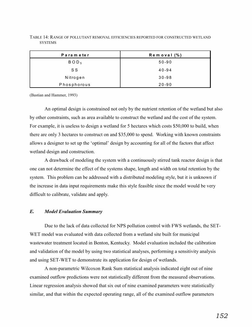
152

TABLE 14: RANGE OF POLLUTANT REMOVAL EFFICIENCIES REPORTED FOR CONSTRUCTED WETLAND

SYSTEMS

P a r a m e te r R e m o v a l (% )

B O D 5 5 0 -9 0

S S 4 0 -9 4

N it ro g e n 3 0 -9 8

P h o s p h o ro u s 2 0 -9 0

(Bastian and Hammer, 1993)

An optimal design is constrained not only by the nutrient retention of the wetland but also

by other constraints, such as area available to construct the wetland and the cost of the system.

For example, it is useless to design a wetland for 5 hectares which costs $50,000 to build, when

there are only 3 hectares to construct on and $35,000 to spend. Working with known constraints

allows a designer to set up the ‘optimal’ design by accounting for all of the factors that affect

wetland design and construction.

A drawback of modeling the system with a continuously stirred tank reactor design is that

one can not determine the effect of the systems shape, length and width on total retention by the

system. This problem can be addressed with a distributed modeling style, but it is unknown if

the increase in data input requirements make this style feasible since the model would be very

difficult to calibrate, validate and apply.

E. Model Evaluation Summary

Due to the lack of data collected for NPS pollution control with FWS wetlands, the SET-

WET model was evaluated with data collected from a wetland site built for municipal

wastewater treatment located in Benton, Kentucky. Model evaluation included the calibration

and validation of the model by using two statistical analyses, performing a sensitivity analysis

and using SET-WET to demonstrate its application for design of wetlands.

A non-parametric Wilcoxon Rank Sum statistical analysis indicated eight out of nine

examined outflow predictions were not statistically different from the measured observations.

Linear regression analysis showed that six out of nine examined parameters were statistically

similar, and that within the expected operating range, all of the examined outflow parameters

153

were within the 95% confidence intervals of the regression lines. A sensitivity analysis showed

the most significant input parameters to the model were those which directly affect bacterial

growth and oxygen uptake and movement. SET-WET was applied to a hypothetical simulation

for the QN2 subwatershed in the Nomini Creek watershed located in Virginia. Various designs

were applied to the area to determine which design parameters had the largest control upon

sediment and nutrient retention at the site. An optimal site design can be made based on the

SET-WET output and constraints from the site. Selecting one ‘optimal’ wetland design depends

on many factors, but when considering nutrient retention only, SET-WET may assist in the

optimization of wetland design.

154

V. Summary, Conclusions, and Recommendations

Constructed wetlands are used as a BMP to alleviate the impact of NPS pollution

problems. Constructed wetlands are an attractive BMP because in addition to controlling NPS

pollutants, they provide other beneficial functions to the environment such as wildlife habitat and

recreation, among others.

One of the more effective ways to enhance the design and implementation of wetlands is

to use computer models. Models provide an ability to make comparisons among alternative

designs and management strategies, thus allowing a wetland to be optimally utilized for its

intended purpose. A model, SET-WET, has been developed which allows these comparisons to

be made.

The SET-WET model is a user-friendly, dynamic, simulation model for design and

evaluation of constructed wetlands in order to optimize NPS pollution control measures.

SET-WET is written in Fortran 77 to facilitate linking with existing NPS models. The model

simulates the hydrologic, N, C, bacteria, DO, vegetative, P and sediment cycles within a wetland

system. The model allows for either free water surface (FWS) or subsurface flow (SSF) wetland

simulations, and is designed in a modular manner; thus it gives the user the flexibility to

concentrate on simulation of specific cycles and processes. The season/time period breakdown

accounts for seasonal variation by allowing the user to change parameter values in the middle of

a simulation run. It allows two forms of data input, one based on measured daily values and

another based on estimates from the SCS curve method in conjunction with runoff concentration

coefficients. Designed as a continuously stirred tank reactor, the model assumes that all

incoming constituents are evenly mixed throughout its entire volume.

The model was calibrated and validated with limited data collected from a constructed

wetland located in Benton, Kentucky. This data was not ideal, as monthly data points needed to

be interpolated to daily values, and the site was designed for wastewater treatment, not NPS

pollution control. Parameter input values were based on previous research and site data. Non-

parametric statistical analyses of the validated results indicated that the predicted hydrologic,

NO3-, NH4

+, organic N, BOD5, TSS, dissolved and total P concentrations were not statistically

different from the measured observations. The Wilcoxon-Rank statistical analyses indicate that

the confidence in the organic N, TSS, and DP predictions were high as the respective p-values

155

approached 1.0. Predictions for DO were consistently higher than observed values, which are a

cause for concern as the DO concentration directly affects many of the bacteria processes.

Linear regression analysis showed that six out of nine examined parameters were statistically

similar, and that within the expected operating range, all of the nine examined outflow

parameters were within the 95% confidence intervals of the regression lines. Due to the limited

amount of data points used for the statistical analyses, results need to be used with caution.

The sensitivity analysis showed that the model was most sensitive to parameters that

directly or indirectly affect bacterial growth or oxygen concentrations in the system. The model

was very sensitive to parameters such as the heterotrophic DO yield and the anaerobic maximum

growth rate in the soil, as values became incomprehensible. In general, however, the NCOB,

sediment and P cycles are relatively insensitive to changes to any single parameter due to the

complexity of the wetland system.

Hypothetical simulations were conducted for design of a possible wetland located in the

QN2 subwatershed of the Nomini Creek watershed in Virginia. The model made predictions on

the nutrient retention of five wetland designs (2.7 hectare, 5.4 hectare, 1.1 hectare, 2 * Plants,

50% Substrate) which when used in conjunction with other constraints (land, ecological,

monetary), a designer would be able to select an optimum design for the wetland. The designed

wetlands reduced the percentage of BOD5 (39.9%-45.5%), TSS (84.5%-99.9%), total N (41.9%-

56.4%), and total P (37.7%-56.5%) to levels reported by previous researchers.

SET-WET differs from many existing wetland models in that it uses a system’s approach,

and limits the assumptions made concerning the interactions of the various nutrient cycles in a

wetland system. It accounts for C and N interactions, as well as for effect of oxygen levels upon

microbial growth. It also directly links microbial growth and death to the consumption and

transformations of nutrients in the wetland system. Many previous models have accounted for

these interactions with zero and first order rate equations that assume rates are dependent only on

initial concentrations.

SET-WET was developed to be as general as possible, but there were assumptions made

during model development which might not apply to all wetland locations. The model assumes

that the FWS system always has free lying surface water, and that the SSF system never floods.

It does not account for snow or snow melt and assumes that the dissolved and particulate

concentrations in both the surface water and substrate water are evenly mixed through the

156

respective volumes. Plant growth is assumed to be of constant composition throughout the

wetland, and is not limited by lack of nutrients or water supply. In addition, growth and death

cannot occur at the same time, and the model does not account for turnover of plant material

during the year. Oxygen transfer by plants is considered to be constant through the growing

season, and it is also assumed that biomass and bacteria prefer nitrate rather than ammonia.

Modeling of adsorption of NH4+ is not conducted as it is assumed that the amount that is

adsorbed is still available for microbial use. The model assumes that P is attached to all of the

particulates in the system based on the surface area of the particles. In addition, SSF wetland

aeration is assumed to be negligible because the water surface is below the substrate, and SSF

wetland PON and POC removal is assumed to be 100% since there are no simple models

available to handle this process.

Through the analysis of the SET-WET model, there are a few suggestions made to

improve the model's predictions. These suggestions concern both laboratory work and improved

model development:

1) There is a need to incorporate a function for sediment resuspension based on the

difference between wetland water velocity and the critical velocity. Sediment

resuspension from the wetland substrate is currently a constant amount whenever the

critical velocity is attained. Another possibility is the use of the ‘overflow rate’ equation

to determine sediment outflow.

2) There is a need for an improved dissolved oxygen model that considers the biomass

oxygenation rate as a function of time. Oxygen is a very sensitive parameter in the SET-

WET model; therefore the assumption of constant rates over the entire growing season

may be limiting the model’s functions.

3) Improve the capabilites of the plant model. There is a need to account for the turnover

ratio of plant life throughout the growing season and not have all death occur only during

a ‘winter’ period.

4) Examine the validity of the assumption that ammonium adsorption is negligible.

157

5) Examine if the modeling of diffusion in the system is quantified properly. Examine if the

diffusion coefficient needs to be a function of time and concentration, instead of a

uniform rate through each season period.

6) Better quantify the initial microbial biomass for HT and AT populations, since the model

is sensitive to these values. In addition, quantify growth parameters in situations that are

more applicable to NPS conditions.

7) Link the model to an existing NPS model, such as ANSWERS, to improve incoming

nutrient flows when the input data is unknown.

8) Extend the model to a series of continuously stirred tank reactors. This would allow the

analysis of wetland length to width ratios, and should allow more accurate predictions of

hydrologic and nutrient effluent.

The SET-WET model takes a novel approach in its attempt to model the constructed

wetland system. It varies from similar models due to its modularity, extreme generality, time

management approach, and the fact that it models both FWS and SSF wetlands. In many ways

this flexibility is the model’s strongest asset, because it provides the model user the ability to

attempt a number of designs for constructed wetlands.

In closing, the SET-WET model is a promising start to modeling FWS constructed

wetlands in a manner that incorporates most of the interactions in a wetland system. There is a

need to further test the model's capabilities, but a useful design tool for both FWS and SSF

constructed wetlands has been developed.

158

VI. Cited Work:

Abtew, W. (1996) Evapotranspiration measurements and modeling for three wetland systems insouth Florida. Water Resources Bulletin 32(3): 465-473

Allen, R. G., M. E. Jensen, J. L. Wright, and R. D. Burman (1989) Operational estimates ofreference evapotranspiration. Agronomy Journal 81: 650-662.

ASTM (1995) Standard practice for evaluating mathematical models for the environmental fateof chemicals. Standard E 978-92, American Society for Testing and Materials, Philadelphia.

Baker, L. A. (1993) Introduction to nonpoint source pollution and wetland mitigation. In:Richard K. Olson (editor), Created and natural wetlands for controlling nonpoint sourcepollution/Office of Wetlands, Oceans, and Watersheds. U.S. Environmental ProtectionAgency, 7-41.

Baker, J. A. (1973) Wetland hydrology. In M. W. Lefor and W. C. Kennard (editors), Proceedingsof the first annual wetlands conference, Storrs, Conn, U Conn, 84-95.

Bastian, R. K., and D. A. Hammer (1993) The use of constructed wetlands for wastewatertreatment and recycling. In: Gerald A. Moshiri (editor), Constructed wetlands for waterquality improvement. Boca Raton: Lewis Publishers, 59-67.

Benefield, L., and F. Molz (1984) Mathematical simulation of a biofilm process. Biotechnologyand Bioengineering 27: 921-931.

Benefield, L. D., J. F. Judkins Jr., and A. D. Parr (1984) Treatment plant hydraulics forenvironmental engineers. Prentice-Hall, Inc., Englewood Cliffs, New Jersey.

Blom, C. W., G. M. Bogemann, P. Laan, A. J. M. Candersman, H. M. vandersteeg, and L. A.Vosenek. (1990) Adaptations to flooding in plants from river areas. Aquatic Botany 38: 29-47.

Bowmer, K. H. (1987) Nutrient removal from effluents by and artificial wetland: Influence ofrhizosphere aeration and preferential flow studied using bromide and dye tracers. WaterResources 21(5): 591-599.

Boyd, C. E. (1978) Chemical composition of wetland plants. In: R. E. Good, D. F. Whigham, andR. L. Simpson (editors). Freshwater wetlands: ecological processes and managementpotential. New York: Academic Press, 155-167.

Brannan, K. (1999) Personal communication: Blacksburg, VA: July, 1999

Brezonik, P. L. (1972) Nitrogen: sources and transformations in natural waters. In: H. E. Allenand J. R. Kramer (editors), Nutrients in natural waters. Wiley –Interface, New York, 1-50.

159

Burns, R. C. and R. W. F. Hardy (1975) Nitrogen fixation in bacteria and higher plants. Springer-Velag, New York, New York.

Chapra, S. C. (1997) Surface water-quality modeling. McGraw-Hill, New York, New York.

Choate, K. D., J. T. Watson, and G. R. Steiner (1990) Demonstration of constructed wetlands fortreatment of municipal wastewaters, monitoring report for the period of March 1998 toOctober 1989. TVA/WR/WQ—90/11, Tennessee Valley Authority.

Christensen, N., W. J. Mitsch, and S. E. Jorgensen (1994) A first generation ecosystem model ofthe Des Plains river experimental wetlands. Ecological Engineering 3: 495-521.

Cowardin, L.M., V. Carter, F. C. Golet, and E. T. Laroe (1979) Classification of wetlands anddeepwater habitats in the United States, U.S. Fish and Wildlife Service pub. FWS/OBS-79/31, Washington, DC.

Costanza, R., and F. H. Sklar (1985) Articulation, accuracy and effectiveness of mathematicalmodels: A review of freshwater wetland applications. Ecological Modelling 27: 45-68.

Cussler, E. L. (1997) Diffusion: mass transfer in fluid systems. Cambridge University Press,United Kingdom.

Daukas, P., D. Lowry, and W. W. Walker Jr. (1989) Design of wet detention basins andconstructed wetland for treatment of stormwater runoff from a regional shopping mall inMassachusetts. In: Donald A. Hammer (editor), Constructed wetlands for wastewatertreatment: municipal, industrial, and agricultural, Lewis Publishers, Inc., Chelsea, Michigan,686-694.

Dennison, M. S., and J. F. Berry (1993) Wetlands: guide to science, law, and technology. NoyesPublications. Park Ridge, New Jersey.

Department of Conservation and Recreation (1996) NPS: nonpoint source pollution and you(brochure). Virginia Department of Conservation and Recreation, Richmond, VA.

Detenback, N. E., and P. L. Brezonik (1991) Phosphorous sorption by sediments from a soft-water seepage lake. 1. An evaluation of kinetic and equilibrium models. EnvironmentalScience and Technology, 25: 395-403.

Dorge, J. (1994) Modeling nitrogen transformations in freshwater wetlands. Estimating nitrogenretention and removal in natural wetlands in relation to their hydrology and nutrient loadings.Ecological Modeling, 75/76:409-420.

Dorge, J. (1998) Personal communication: Blacksburg, VA: September, 1998.

160

Dierberg, F. E., and P. L. Brezonik (1984) Nitrogen and phosphorous mass balances in a cypressdome receiving wastewater. In: K. C. Ewel and H. T. Odum (editors), Cypress swamps.Gainesville, University of Florida Press, 112-118.

Dillaha, T. A. (1990) Role of best management practices in restoring the health of theChesapeake Bay. In: Perspectives on the Chesapeake Bay, 1990: Advances in EstuarineSciences. Chesapeake Bay Program, USEPA, Washington, DC CBP/TRS41/90.

Duever, M. J. (1988) Hydrologic processes for models of freshwater wetlands. In : W.J. Mitsch,M. Straskraba and S. E. Jorgensen (editors), Wetland Modelling, Elsevier, Amsterdam, 9-39.

Environmental Law Institute, Wetlands deskbook. (Washington, D.C.: author) pg. 18.

EPA (1988) Constructed wetlands and aquatic plant systems for municipal wastewater treatment:Design manual EPA/625/1-88/022. Washington, DC: Office of research and development.

Fennessy, M. S., C. C. Brueske, and W. J. Mitsch (1994) Sediment deposition patterns in restoredfreshwater wetlands using sediment traps. Ecological Engineering 3:409-428.

Fetter, C. W. (1994). Applied hydrogeology. Prentice Hall, Upper Saddle River, New Jersey.

Fields, S. (1993) Regulations and policies relating to the use of wetlands for nonpoint sourcecontrol. In: Richard K. Olson (editor), Created and natural wetlands for controlling nonpointsource pollution/Office of Wetlands, Oceans, and Watersheds. U.S. Environmental ProtectionAgency, 151-158.

French, R. H. (1984) Lake modeling: state of the art. Critical Reviews in EnvironmentalChemistry. 13(4): 311-357.

Fyock, O. L. (1977) Nitrification requirements of water reuse systems for rainbow trout.Colorado Division of Wildlife, Fisheries Research Section, No. 41; February 1977.

Gambrell, R. P. and W. H. Patrick Jr. (1978) Chemical and microbiological properties ofanaerobic soils and sediments. In: D.D. Hook and R. M. M. Crawford (editors), Plant Life inAerobic Environments, Ann Arbor Sci. Pub. Inc., Ann Arbor Michigan, 375-423.

Gidley, T. M. (1995) Development of a constructed subsurface flow wetland simulation model.MS Thesis, North Carolina State, pp. 139.

Good, R. E., D. F. Whigham, and R. L. Simpson. (1978) Freshwater wetlands: ecologicalprocesses and management potential. Academic Press, New York, New York.

Grady Jr., C. P. L. and H. C. Lim. (1980) Biological wastewater treatment – theory andapplications. New York: Marcel Dekker Inc.

161

Guardo, M., and R. S. Tomasello (1995) Hydrodynamic simulations of a constructed wetland inSouth Florida. Water Resources Bulletin, 31(4): 687-701.

Hales, L. Z., S. L. Bird, B. A. Ebersole, and R. Walton (1990) Bolsa Bay, California, proposedocean entrance system. Tidal circulation and transport computer simulation and waterquality assessment. U.S. Army Engineer Waterways Experiment Station. Vicksburg, MS,USA. Report 3.

Hammer, D. H., and R. H. Kadlec (1986) A model for wetland surface water dynamics. WaterResources Research, 22(13) 1951-1958.

Hart, B. T. (1982) Uptake of trace metals by sediment and suspended particles: a review.Hydrbiologia, 91:299-313.

Hatano, K, D. J. Frederick, and J.A. Moore (1994) Microbial ecology of constructed wetlandsused for treating pulp mill wastewater. Water Science and Technology, 29(4) 233-239.

Heatwole, C. D. (1988) Class Notes from BSE 5354: NPS modeling. Virginia PolytechnicInstitute and State University, BSE Department.

Henze, M., C. P. L. Grady Jr., W. Gujer, G, v, R, Marias, and T. Matsuo (1986) Activated sludgemodel no. 1. In: IAWPRC scientific and technical reports No. 1. IAWPRC task group onmathematical modeling for design and operation of biological wastewater treatment.

Hey D. L., M. A. Cardamone, J. H. Sather, and W. J. Mitsch (1989) In: W. J. Mitsch and S. E.Jorgensen (editors), Ecological engineering, an introduction to ecotechnology, John Wiley &Sons, New York, 159-183.

Hosokawa, Y. and K. Furukawa (1994) Surface flow and particle settling in a coastal reed field.Water Science and Technology, 29(4) 45-53.

Hosokowa, Y, and T Horie (1992) Flow and particulate nutrient removal by wetland withemergent macrophyte. Science and total environment, supplement; 1271-1282.

Jansson, S. L. and J. Persson (1982) Mineralization and immobilization of soil nitrogen. In: F. J.Stevenson (editor). Nitrogen in agricultural soils. Madison, WI: American Society ofAgronomy, Inc., Crop Science Society of America, Inc., and Soil Science Society of AmericaInc., 229-252.

Johnson, C. A., G. D. Bubezner, G. B. Lee, F. W. Madison, and K. R. McHenry (1984) Nutrienttrapping by sediment deposition in a seasonally flooded lakeside wetland. A Landscapeapproach. Biogeochemistry, 10: 105-141.

Johnston, C. A. (1991) Sediment and nutrient retention by freshwater wetlands: effects onsurface water quality. Critical reviews in environmental control 21(5-6), 491-565.

162

Jorgensen, S. E. (1983) Application of ecological modelling in environmental management, partA. Elsevier Scientific Publishing Company. New York, New York.

Jorgensen, S. E. (1989) Sedimentation. In S.E. Jorgensen and M.J. Gromiec (editors),Mathematical submodels in water quality systems. Elsevier, Amsterdam.

Jorgensen, S. E. (1995) State-of-the-art management models for lakes and reservoirs. Lakes andreservoirs: research and management. 1:79-87.

Jorgensen, S. E., C. C. Hoffman, and W. J. Mitsch (1988) Modeling nutrient retention by areedswamp and wet meadow in Denmark. . In : W.J. Mitsch, M. Straskraba and S. E.Jorgensen (editors), Wetland modelling, Elsevier, Amsterdam, 133-151.

Kadlec, R.H., and D. E. Hammer (1988) Modeling nutrient behavior in wetlands. EcologicalModelling, 40:37-66.

Kadlec, R. H. (1989a) Hydrologic factors in wetland water treatment. In: Donald A. Hammer(editor), Constructed wetlands for wastewater treatment: municipal, industrial, andagricultural, Lewis Publishers, Inc., Chelsea, Michigan, 21-40.

Kadlec, R. H. (1989b) Decomposition in wastewater wetlands. In: Donald A. Hammer (editor),Constructed wetlands for wastewater treatment: municipal, industrial, and agricultural, LewisPublishers, Inc., Chelsea, Michigan, 459-468.

Kadlec, R. H. (1990) Overland flow in wetlands: vegetation resistance. Journal of hydraulicengineering, 116(5):691-706

Kadlec, R.H. and R.L. Knight. (1996). Treatment wetlands. CRC Lewis Publishers. Boca Raton,Florida.

Kadlec, R. H. (1997) An autobiotic wetland phosphorous model. Ecological Engineering 8: 145-172.

Kulin, G., and P. R. Compton (1975) A guide to methods and standards for the measurement ofwater flow: Special publication 421, National Bureau of Standards.

Loague, K. and R. E. Green (1991) Statistical and graphical methods for evaluating solutetransport models: Overview and application. Journal of Contaminant Hydrology 7: 51-73.

McCarty, P.L. (1975) Stoichiometry of biological reactions. Progress in Water Technology 7:157-172.

Mitsch, W.J. (1988) Productivity-hydrology nutrient models of forested wetlands. In: W.J.Mitsch, M. Straskraba and S. E. Jorgensen (editors), Wetland modelling, Elsevier,Amsterdam, 115-132.

163

Mitsch, W. J., and J. G. Gosselink (1986) Wetlands. Van Nostrand Reinhold. New York, NewYork.

Mitsch, W. J., and J. G. Gosselink (1993) Wetlands. Van Nostrand Reinhold. New York, NewYork.

Mitsch, W. J., J. K. Cronk, X. Wu, R. W. Nairn, and D. L. Hey (1995) Phosphorous retention inconstructed freshwater riparian marshes. Ecological Applications, 5(3):830-845.

Mitsch, W.J., and B. C. Reeder. (1991) Modelling nutrient retention of a freshwater coastalwetland: estimating the roles of primary productivity, sedimentation, resuspension, andhydrology. Ecological modelling 54:151-187.

Mostaghimi, S., S. Shukla, and P. W. McClellan (1998) BMP Impacts on nitrate and pesticidetransport to groundwater in the Nomini creek watershed: Report No. NC-0298.

Niswander S. F., and W. J. Mitsch (1995) Functional analysis of a two-year old created in-streamwetland: Hydrology, phosphorus retention, and vegetation survival and growth. Wetlands,15(3):212-225.

Novotny, V. and G. Chesters (1981) Handbook of nonpoint source pollution sources andmanagement. Van Nostrand Reinhold Company. New York, New York.

Novotny, V., and H. Olem (1994) Water quality: prevention, identification and management ofdiffuse pollution. Van Nostrand Reinhold. New York, New York.

Ott, R. L. (1993) An introduction to statistical methods and data analysis. Duxbury Press.Belmont, CA.

Perrich, J. R. (1981) Activated carbon adsorption for wastewater treatment. CRC Press, Inc.Boca Raton, FL.

Raisin, G. W. and D. S. Mitchell (1995) The use of wetlands for the control of non-point sourcepollution. Water, Source and Technology, 32(3): 177-186.

Reddy, K. R., Khaleel, R., Overcash, M. R., and P. W. Westerman (1979) A nonpoint sourcemodel for land areas receiving animal wastes. I: Mineralization of organic nitrogen.Transactions of the ASAE 22: 863.

Reddy, K. R. (1982) Mineralization of nitrogen in organic soils. Soil Sci. Soc. Am. J., 46(3):561-566.

Reddy, K. R. and W. H. Patrick (1984) Nitrogen transformations and loss in flooded soils andsediments. CRC Critical Reviews in Environmental Control, 13(4): 273-309.

164

Reed, S. C. (1994) Design of subsurface flow constructed wetland for wastewater treatment. In:S. C. Reed, E. J. Middlebrooks, and R. W. Crites (editors). Natural systems for wastemanagement and treatment, 2nd Edition. New York, McGraw and Hill.

Ruffner, J. A. (1980) Climates of the states, Volume 2. Gale Research, Detroit, Michigan.

Salvesen, D. (1994) Wetlands: mitigating and regulating development impacts. Second edition.Washington D.C.: ULI – the Urban Land Institute.

Shaw, S. P., and C. G. Fredine (1956) Wetlands of the United States, their extent, and their valuefor waterfowl and other wildlife. U.S. Department of Interior, Fish and Wildlife Service,Circular 39, Washington D.C.

Silverman, G. S. (1989) Treatment of nonpoint source pollutants – urban runoff and agriculturalwastes: Development of urban runoff treatment wetlands in Fremont, California. In: DonaldA. Hammer (editor), Constructed wetlands for wastewater treatment: municipal, industrial,and agricultural, Lewis Publishers, Inc., Chelsea, Michigan, 669-676.

Soil Conservation Service (1968) Hydrology, supplement A to sec.4, Engineering Handbook,USDA-SCS, Washington D.C.

Snoeyink, V. L., and D. Jenkins (1980) Water chemistry. John Wiley & Sons, New York, NewYork.

Tanji K. K. (1982) Modeling of the soil nitrogen cycle. In: F. J. Stevenson (editor). Nitrogen inagricultural soils. Madison, WI: American Society of Agronomy, Inc., Crop Science Societyof America, Inc., and Soil Science Society of America Inc., 721-772.

Tanner, C. C. (1996) Plants for constructed wetland treatment systems – A comparison of thegrowth and nutrient uptake of eight emergent species., Ecological Engineering (7) 59-83.

Tchobangolous, G. and F. L. Burton (1991) Wastewater engineering: treatment, disposal andreuse. Third edition. New York: Metcalf and Eddy, Inc. McGraw-Hill, Inc.

Teague L. L., A. L. Kenimer, B. J. Lesker, and F. L. Mitchell (1997) Constructed wetlands for thecontrol of agricultural nonpoint source pollution. ASAE Paper No. 972037

Tiner Jr., R. W. (1984) Wetlands of the United States: current status and recent trends, NationalWetlands Inventory Project. U.S. Fish and Wildlife Service.

USDA, Soil Conservation Service (1988) National handbook of conservation practices.Washington, D. C.

USEPA (1993) Created and natural wetlands for controlling nonpoint source pollution. BocaRaton: Smoley C.K.

165

USSCS (1975) Soil taxonomy: A basic system of soil classification for making and interpretingsoil surveys. U. S. Soil Conservation Service Agricultural Handbook 436. Washington, D.C.

Urban, N. R., and S. J. Eisenreich (1988) Nitrogen cycling in a forested Minnesota bog.Canadian Journal of Botany, 66: 435-449.

Walton, R., R. S. Chapman, and J. E. Davis (1996) Development and application of the wetlandsdynamic water budget model. Wetlands, 16(3): 347-357.

Watson, J. T., Sherwood, C. R., Kadlec, R. H., Knight, R. L., and A. E. Whitehouse (1989)Performance expectation and loading rates for constructed wetlands. In: Donald A. Hammer(editor), Constructed wetlands for wastewater treatment: municipal, industrial, andagricultural, Lewis Publishers, Inc., Chelsea, Michigan, 319-351.

Wheaton, F., J. Hochheimer, and G.E. Kaiser (1991) Fixed film nitrification filters foraquaculture. In: Brune, D.E. and J. R. Tomasso (editors), Aquaculture and Water Quality.Baton Rouge, LA: The World Aquaculture Society, 272-303.

Whitaker, G., and C. R. Terrell (1993) Federal programs for wetland restoration and use ofwetlands for nonpoint source pollution control. In: Richard K. Olson (editor), Created andnatural wetlands for controlling nonpoint source pollution/Office of Wetlands, Oceans, andWatersheds. U.S. Environmental Protection Agency, 201-215.

Widener, A. S. (1995) A mathematical model of the nitrogen cycle in a constructed wetland. MSThesis, Virginia Polytechnic Institute and State University. pp. 145.

Wood. R. A. (1996) The weather almanac. Gale research, Detroit, MI.

Zak, D. R. and D. F. Grigal (1991) Nitrogen mineralization, nitrification, and denitrification in

upland and wetland ecosystems. Oegologia, 88: 189-196.

166

VII. Appendices

167

Appendix A: Model Parameters

List of all model parameters for SET-WET. In the following table, inputs have their first lettercapitalized, stocks are entirely capitalized, while any flows or parameters which are determinedby SET-WET are entirely lower case.

MODELCOMPONENT DESCRIPTION UNITS

Abioremd Amount of standing dead biological mass removal g biomass/dayAbioreml Amount of living biological mass removal g biomass/day

Adsorp Type of adsorption model used -

AemaxgrbAerobic heterotroph maximum growth rate at optimal conditions in peat water day-1

AemaxgrwAerobic heterotroph maximum growth rate at optimal conditions in surface water day-1

aerohtgb growth of bottom aerobic heterotrophs g microbes/dayaerohtgw growth of surface aerobic heterotrophs g microbes/dayAirtemp Ambient Air Temperature degrees CAlpha Kadlec equation (slope exponent) -

ammupb plant ammonium uptake from wetland bottom g N/ dayammupw plant ammonium uptake from wetland surface g N/ day

anfracbfraction of heterotrophs that are anaerobes - function of DO conc. in bottom

g anaerobic HT/ g total HT

anfracwfraction of heterotrophs that are anaerobes - function of DO conc. in surface

g anaerobic HT/ g total HT

Angvnot Angle of weir notch (outlet=2) degrees anhtgb growth of bottom anaerobic heterotrophs g microbes/dayanhtgw growth of surface anaerobic heterotrophs g microbes/day

AnmaxgrbAnaerobic heterotroph maximum growth rate at optimal conditions in peat water day-1

AnmaxgrwAnaerobic heterotroph maximum growth rate at optimal conditions in surface water day-1

Apflow amount of point flow contribution (point=1) m3/day

Areapipe Area of outflow pump (outlet=3) m2

Atdep Atmospheric Deposition (0=not include, 1=include)Beta Kadlec equation (depth exponent)

Bioccont Fraction of carbon in plants g C/ g biomass

biodegrstanding dead degradation rate - set for 99% over the course of a year - converted to POC day-1

Biodens Living biomass density kg/m3

biofluxb oxygen flux from rootzone aeration by plants g O2/day

Bioinit Initial total plant mass g Plant BIOMASS total plant carbon mass g C

BIOMASST total biomass in the wetland system g biomassbiomassv volume of biomass g biomassBiomcn Ratio of carbon to nitrogen in plants g C/g Nbiomdth biomass death g biomass/day

biomgrow biomass growth g biomass/day

Biomgrr Rate at which plants grow

g biomass/

m2-daybiomout amount of biomass removal for external reasons g biomass/day

168


Biompn Ratio of plant mass to nitrogen in plants g plant mass/g N

Biompp Biomass plant/phosphorous ratiog plant/g

phosphorous

Biooxrbrate at which oxygen is added to the rootzone by plants gO2 /m2*day

BioremdRemoval of dead biomass biological material (0=no removal for stress period, 1=removal) -

BioremlRemoval of live biomass biological material (0=no removal for stress period, 1=removal) -

BocconcInfluent BOD5 concentration in point source additions mg BOD5/L

Bocdinfco Influent BOD5 concentration in water additions mg BOD5/LBodcfrac Fraction of carbon in influent BOD g C/g BOD5

Bodpfrac Fraction of influent BOD which is in particulate formg. part. BOD5/ g

total BOD5Bodrc BOD runoff coefficient mg BOD5/L

btphos amount of bottom particulate phosphorous attached to each respective sediment category g PP

BtphosiInitial amount of total particulate phosphorous in wetland bottom water pool g P-phos

BTPHOST total particulate phosphorous in wetland bottom g PP

check (1-7)Flag to determine entry of data between changing stress periods -

Coefk Kadlec equation (premultiplier constant) -Contc Pipe contraction coefficient (outlet=3) -

Daddon Dry atmospheric deposition rate for DON g DON/m2

Dadnh4 Dry atmospheric deposition rate for NH4 g NH4/m2

Dadno3 Dry atmospheric deposition rate for NO3 g NO3/m2

Dadpon Dry atmospheric deposition rate for PON g PON/m2

Daylen fraction of 24 hour day between sunrise and sunset hours daylight/12

Dayremd Removal date of material day of season

period

Dayreml Removal date of material day of season

periodDaysdeg Time frame over which plant biomass degrades days

Daywins Day when winter starts in time periodday of season

period

Daywine Day when winter ends in season periodday of season

period

deadphosamount of PP entering system from plant physical degradation per category g PP/day

deadphottotal amount of PP entering system from plant physical degradation g PP/day

deathbtransfer of immobilized nitrogen to bottom PON due to death of bottom microbes or plants g N/day

deathwtransfer of immobilized nitrogen to surface PON due to death of surface microbes or plants g N /day

Decompdecomposition rate of organic material in wetland bottom

g deg. SS/ g SS

Degbio Point to which biomass will degrade % degradation

169


deltahtchange in wetland bottom height due to peat accumulation, sediment resuspension/settling m

denitbconversion of bottom nitate to N2 gas by bottom anaerobic heterotrophs g N/ day

denitwconversion of surface nitate to N2 gas by surface anaerobic heterotrophs g N/ day

Diseffc Effective discharge coefficient mdisphosc DP watershed runoff inflow concentration mg DP/L

DisphoscDissolved phosphorous inflow concentrations from catchment mg/l

disphosi total amount of DP entering wetland system g DP/dayDOCB amount of dissolved organic carbon in bottom g Cdoccb dissolved organic carbon concentration in bottom mg DOC/Ldoccw dissolved organic carbon concentration in surface mg DOC/L

Docininc DOC concentration for percolating sources mg C/L

DocinitbInitial amount of dissolved organic carbon in peat water g C

DocinitwInitial amount of dissolved organic carbon in surface water g C

docleach leaching of DOC from standing dead to DOC g C/ day

docminibconversion of bottom DOC to microbial biomass and carbon dioxide g C/day

docminiwconversion of surface DOC to microbial biomass and carbon dioxide g C/day

docmt DOC mass transfer g C/dayDoconcin Dissolved oxygen concentration in water input mg O2/LDoconcp Oxygen concentration in precipitation mg O2/L

docout effluent DOC flux g C/daydocperc DOC percolation/infiltration to/from wetland bottom g C/dayDOCW amount of dissolved organic carbon in surface g Cdoinf dissolved oxygen additions from watershed runoff g O2/day

Doinitb Total mass of oxygen in the peat water g O2Doinitw Total mass of oxygen in the surface water g O2

donammbconversion of excess DON to ammonium by bottom heterotrophic bacteria during organics degradation g N/ day

donammwconversion of excess DON to ammonium by surface heterotrophic bacteria during organics degradation g N/ day

donat DON contributed by atmospheric deposition g DON/ dayDONB amount of dissolved organic nitrogen in bottom g DONdoncb dissolved organic nitrogen concentration in bottom mg DON/L

Donconc DON concentration in point flow mg DON/Ldoncw dissolved organic nitrogen concentration in surface mg DON/Ldonec DON effleunt concentration g N/l

donimmbincorporation of DON by bottom heterotrophic microbes during organics decomposition g N /day

donimmwincorporation of DON by surface heterotrophic microbes during organics decomposition g N /day

donin incoming DON from watershed runoff additions g N/dayDonininc DON concentration from percolating source mg DON/L

170


Doninitb Initial dissolved organic nitrogen in peat water g NDoninitw Initial dissolved organic nitrogen in surface water g N

donminb

conversion of excess bottom DON to ammonium by bottom heterotrophic bacteria during organics degradation g N/day

donminw

conversion of excess surface DON to ammonium by surface heterotrophic bacteria during organics degradation g N/day

donmt mass transfer of DON between surface and bottom g DON/daydonout effluent DON flux g N/day

donperc DON percolation/infiltration from bottom g DON/dayDONW amount of dissolved organic nitrogen in surface g DON/daydoout effluent disolved oxygen flux g O2/day

doperc percolation/infiltration of DO from wetland bottom g O2/day

DOXYB amount of dissolved oxygen in wetland bottom g O2Doxycsat DO saturation constant mg O2/L

DOXYW amount of dissolved oxygen in wetland surface g O2

dphosec Effluent dissolved phosphorous concentration mg DP/Ldphosout effluent dissolved phosphorous flux g DP/dayDTPHOSB total dissolved phosphorous in wetland bottom g DPdtphoscb Dissolved phosphorous concentration for bottom mg DP/Ldtphoscw Dissolved phosphorous concentration for surface mg DP/L

DtphosibInitial amount of dissolved phosphorous in wetland bottom water pool g DP

DtphosiwInitial amount of dissolved phosphorous in wetland surface water pool g DP

DTPHOSW total dissolved phosphorous in wetland surface g DPEvap Evaporation model (0=Thornthwaite, 1=pan) -

evapcoefcalculated climate parameter for Thornthwaite's ET method -

Evapt Amount of evaporation from wetland cell m3/day

evapt water loss due to evapotranspiration m3

evapttamount of water loss due to evapotranspiration for hourly time step m3/hour

fixnitamount of atmospheric nitrogen converted to DON by microbes g ON/day

Flowout Amount of water removed (outlet=4) m3/day

flowratecalculated parameter for SCS curve method - amount of surface runoff mm

Freundk Freundlich isotherm constant -Freundn Freundlich isotherm constant -

Hb Bottom of peat component in wetland cell m

heatijcalculated climate parameter for Thornthwaite's ET method -

heatindxcalculated climate parameter for Thornthwaite's ET method -

HETEROB amount of heterotrophs in bottom g microbes

171


HeteroibInitial total mass of heterotrophic bacteria in peat water g microbes

HeteroiwInitial total mass of heterotrophic bacteria in surface water g microbes

HETEROW amount of heterotrophs in surface g microbes Hii Initial height of water in wetland cell relative to (z=0) mhit wetland surface water height for hourly time step m

hnh4immb

bottom ammonium nitrogen utilized by bottom heterotrophic bacteria during organics degradation g NH4+-N/day

hnh4immw

surface ammonium nitrogen utilized by surface heterotrophic bacteria during organics degradation g NH4+-N/day

Hno3hscbAnaerobic heterotroph nitrate half saturation constant for peat water mg NO3--/L

Hno3hscwAnaerobic heterotroph nitrate half saturation constant for surface water mg NO3--/L

Ho Top of wetland cell m

HorghscbHeterotroph organics half saturation constant for peatwater mg C/L

HorghscwHeterotroph organics half saturation constant for surface water mg C/L

HoutHeight of overflow for outlet option (outlet=1, 2 , 3 ,4, or 6) m

Hover Height for water overflow of weir (outlet=1) mhrt hydraulic residence time days

htdeathb death of bottom heterotrophs g microbes/dayhtdeathw death of surface heterotrophs g microbes/day

HtdohscbAerobic heterotroph dissolved oxygen half saturation constant in surface water mg O2/L

HtdohscwAerobic heterotroph dissolved oxygen half saturation constant in peat water mg O2/L

Htdoyb Oxygen yield of aerobic heterotrophs in peat water g microbes/g O2

HtdoywOxygen yield of aerobic heterotrophs in surface water g microbes/g O2

Htdrb Heterotroph death rate in peat water g microbes/dayHtdrw Heterotroph death rate in surface water g microbes/day

htgrowb growth of bottom heterotrophs g microbes/dayhtgroww growth of surface heterotrophs g microbes/day

Hti Top of peat component in wetland cell m

Htno3y Nitrate yield of anaerobic heterotrophsg microbes/

g NO3--N

htrespb bottom oxygen loss by bottom heterotroph growth g O2/day

htrespw surface oxygen loss by surface heterotroph growth g O2/day

httempfbHeterotroph bottom temperature factor - reduces growth rate at nonoptimal conditions -

httempfwHeterotroph surface temperature factor - reduces growth rate at nonoptimal conditions -

htyieldb yield of bottom heterotrophic microbesg microbes/ g C

degraded

htyieldw yield of surface heterotrophic microbesg microbes/ g C

degraded

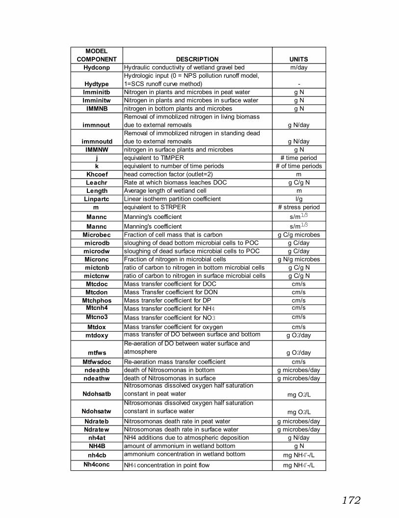
172


Hydconp Hydraulic conductivity of wetland gravel bed m/day

HydtypeHydrologic input (0 = NPS pollution runoff model, 1=SCS runoff curve method) -

Imminitb Nitrogen in plants and microbes in peat water g NImminitw Nitrogen in plants and microbes in surface water g N

IMMNB nitrogen in bottom plants and microbes g N

immnout Removal of immoblized nitrogen in living biomass due to external removals g N/day

immnoutdRemoval of immoblized nitrogen in standing dead due to external removals g N/day

IMMNW nitrogen in surface plants and microbes g Nj equivalent to TIMPER # time periodk equivalent to number of time periods # of time periods

Khcoef head correction factor (outlet=2) mLeachr Rate at which biomass leaches DOC g C/g NLength Average length of wetland cell m

Linpartc Linear isotherm partition coefficient l/gm equivalent to STRPER # stress period

Mannc Manning's coefficient s/m1/3

Mannc Manning's coefficient s/m1/3

Microbec Fraction of cell mass that is carbon g C/g microbesmicrodb sloughing of dead bottom microbial cells to POC g C/daymicrodw sloughing of dead surface microbial cells to POC g C/dayMicronc Fraction of nitrogen in microbial cells g N/g microbesmictcnb ratio of carbon to nitrogen in bottom microbial cells g C/g Nmictcnw ratio of carbon to nitrogen in surface microbial cells g C/g NMtcdoc Mass transfer coefficient for DOC cm/sMtcdon Mass Transfer coefficient for DON cm/s

Mtchphos Mass transfer coefficient for DP cm/sMtcnh4 Mass transfer coefficient for NH4 cm/s

Mtcno3 Mass transfer coefficient for NO3 cm/s

Mtdox Mass transfer coefficient for oxygen cm/smtdoxy mass transfer of DO between surface and bottom g O2/day

mtfws

Re-aeration of DO between water surface and atmosphere g O2/day

Mtfwsdoc Re-aeration mass transfer coefficient cm/sndeathb death of Nitrosomonas in bottom g microbes/dayndeathw death of Nitrosomonas in surface g microbes/day

NdohsatbNitrosomonas dissolved oxygen half saturation constant in peat water mg O2/L

NdohsatwNitrosomonas dissolved oxygen half saturation constant in surface water mg O2/L

Ndrateb Nitrosomonas death rate in peat water g microbes/dayNdratew Nitrosomonas death rate in surface water g microbes/day

nh4at NH4 additions due to atmospheric deposition g N/dayNH4B amount of ammonium in wetland bottom g N

nh4cb ammonium concentration in wetland bottom mg NH4+-/L

Nh4conc NH4 concentration in point flow mg NH4+-/L

173


nh4cw ammonium concentration in wetland surface mg NH4+-/L

nh4ec NH4 effluent concentration mg NH4+-/L

nh4in ammonium flux from watershed runoff additions -Nh4inc NH4 influent concentration mg NH4+-/L

Nh4ininc NH4 concentration from percolating source mg NH4+-/L

Nh4initbInitial ammonia and ammonium nitrogen in peat water g NH4

Nh4initwInitial ammonia and ammonium nitrogen in surface water g NH4

nh4mtmass transfer og ammonium between surface and bottom g N/ day

nh4out effluent NH4 flux g N/daynh4perc NH4 percolation/infilitration from wetland bottom g N/day

Nh4rc NH4 runoff coefficient mg NH4+-/L

NH4W amount of ammonium in wetland surface g NNitcycle Nitrogen Cycle (0=not included, 1=included) -

Nitfix Nitrogen fixation (0=not included, 1=included) -

Nitfrate Nitrogen fixation rate g DON/ (day*m2)

nitrifbconversion of ammonium to nitrate by bottom autotrophs g N /day

nitrifwconversion of ammonium to nitrate by surface autrotrophs g N /day

NitrosibInitial total mass of Nitrosomonas sp. Autotrophic bacteria in peat water g microbes

NitrosiwInitital total mass of Nitrosomonas sp. Autotrophic bacteria in surface water g microbes

NITROSOB amount of Nitrosomonas in bottom g microbes NITROSOW amount of Nitrosomonas in surface g microbes

nitupb plant nitrate uptake from wetland bottom g N/ daynitupw plant nitrate uptake from wetland surface g N/ daynleach nitrogen leached from standing dead to DON g N/day

NmaxgrbNitrosomonas maximum growth rate at optimal conditions in peat water day-1

NmaxgrwNitrosomonas maximum growth rate at optimal conditions in surface water day-1

Nnh4hscbNitrosomonas ammonium half saturation constant for peat water mg NH4+-/L

Nnh4hscwNitrosomonas ammonium half saturation constant for surface water mg NH4+-/L

no3at NO3 additions due to atmospheric deposition g N/dayNO3B amounf of nitrate in wetland bottom g N

no3cb nitrate concentration in wetland bottom mg NO3--/L

No3conc NO3 concentration in point flow mg NO3--/L

no3cw nitrate concentration in wetland surface mg NO3--/L

no3ec effluent nitrate concentration mg/lno3in influent nitrate flux from watershed runoff g N/day

No3inc NO3 influent concentration mg NO3--/L

No3ininc NO3 concentration from percolating source mg NO3--/LNo3initb Initial oxidized nitrogen in peat water g NO3

174


No3initw Initial oxidized nitrogen in surface water g NO3

no3mt mass transfer of NO3 between surface and water g N/day

no3out effluent nitrate flux mg NO3--/L

no3perc NO3 percolation/infiltration from wetland bottom g N/dayNo3rc NO3 runoff coefficient mg NO3--/L

NO3W amount of nitrate in wetland surface g N

NsdoybOxygen yield of Nitosomonas bacteria in surface water g microbes/g O2

NsdoywOxygen yield of Nitosomonas bacteria in surface water g microbes/g O2

nsgrowb growth of Nitrosomona in bottom g microbes/daynsgroww growth of Nitrosomonas in surface g microbes/daynsrespb bottom oxygen loss by bottom autotroph growth g O2/day

nsrespw surface oxygen loss by surface autotroph growth g O2/day

nstempfbNitrosomonas bottom temperature factor - reduces growth rate at nonoptimal conditions -

nstempfwNitrosomonas surface temperature factor - reduces growth rate at nonoptimal conditions -

Nsyieldb Yield of Nitrosomas bacteria in peat waterg microbes/ g

NH4+-N

Nsyieldw Yield of Nitrosomas bacteria in surface waterg microbes/ g

NH4+-N

Numstper Number of stress periods in simulation run # of periodsNumtmper Number of time periods for respective stress period # time steps

Onpartf Fraction of organic nitrogen in particulate form g PON/g TONOrgininc Organic nitrogen influent concentration mg ON/LOrgnrc Organic nitrogen runoff coefficient mg ON/L

Outflow effluent flowrate m3/day

outflow effluent water flux m3/day

outflowt effleunt water flux for hourly time step m3/hourOutlet Outlet type (6 options) -

Outwidth Width of outflow weir (outlet=1) mOxyconc Oxygen concentration from point flow mg O2/L

Oxyrc Runoff coefficient for oxygen mg O2/L

Panevap Pan Evaporation Rate m/day

Pbiouw Percentage of living biomass which is underwater% mass

underwater pbodin particulate BOD flux from watershed runoff additions g C/dayPcycle Phosphorus cycle (0=not included, 1=included) -

PeatacrbRate at which refractory solids accumulate in the peat water g solids/day

PeatacrwRate at which refractory solids accumulate in the surface water g solids/day

peatcacb rate at which bottom refractory solids accumulate g C/daypeatcacw rate at which surface refractory solids accumulate g C/day

Peatcc Fraction of carbon in refractory solids g C/g solids

Peatdens Density of peat material kg/m3

peatnacb nitrogen in accumulating bottom refractory solids g N /day

175


peatnacw nitrogen in accumulating surface refractory solids g N /dayPeatnc Fraction of nitrogen in accumulated solids g N/g solids

Percinf Percolation or Infiltration additions (0=no,1=yes)Percinfa Percolation/Infiltration rate for stress period m/day

percinftpercolation/infiltration gains/losses to/from wetland bottom m3

percittamount of percolation/infiltration changes for hourly time step m3/hour

Ph pH of water in wetland system pHphdep pH factor for volatilization -

PhosconIncoming amount of dissolved phosphorous from point source additions g DP/day

phosmt mass transfer of DP from surface and bottom g DP/day

phosperattachment ratio for incoming phosphorous to respective sediment categories -

phosperbratio of phosphorous attachment upon bottom sediment -

phosperbattachment ratio for bottom phosphorous to respective sediment categories -

phosperwattachment ratio for surface phosphorous to respective sediment categories -

phosupb plant uptake of DP from bottom g DP/dayphosupw plant uptake of DP from surface g DP/dayphysdeg degradation of standing dead to refractory material g biomass/dayphysdegc conversion of standing dead to plants to POC g C/day

PinincDissolved phosphorous concentration for percolating water source mg DP/L

pminpp phosphorous remineralization from surface particulate pool for individual sediment category g DP/day

Pminppc Mineralization rate from surface particulate pool day-1

pminppttotal amount of remineralization from surface particulate pool g PP/day

POCB amount of POC in bottom g C/daypoccb particulate organic carbon concentration in bottom mg POC/Lpoccw particulate organic carbonconcentration in surface mg POC/LPocfall POC Fallling rate m/day

PocinitbInitial amount of particulate organic carbon in surface water g C

PocinitwInitial amount of particulate organic carbon in peat water g C

pocminibconversion of bottom POC to microbial biomass and carbon dioxide g C/day

pocminiwconversion of surface POC to microbial biomass and carbon dioxide g C/day

pocout effluent POC flux g C/daypocre POC resuspension form wetland bottom g C/day

Pocres POC resuspension rate ratio

% (g POC resuspended/g POC in peat)

pocset settling of surface POC to wetland bottom g C/dayPocsize Average size of particulate organic carbon mm

176


POCW amount of POC in surface g C/dayPoint Point flow addition (0=no, 1=yes) -

ponammb

conversion of excess bottom PON to ammonium by bottom heterotrophic bacteria during organics degradation g N/day

ponammw

conversion of excess surface PON to ammonium by surface heterotrophic bacteria during organics degradation g N/day

ponat PON additions due to atmospheric deposition g N/dayPONB amount of PON in wetland bottom g N/dayponcb particulate organic nitrogen concentration in bottom mg PON/L

Ponconc PON concentration in point flow mg PON/Lponcw particulate organic nitrogen concentration in surface mg PON/Lponec effluent PON concentration mg PON/LPonfall PON fall rate m/d

ponimmbincorporation of bottom PON by bottom heterotrophic bacteria during organics degradation g N/day

ponimmwincorporation of surface PON by surface heterotrophic bacteria during organics degradation g N/day

ponin particulate organic nitrogen flux from watershed g N/dayPoninitb Initial particulate organic nitrogen in peat water g NPoninitw Initial particulate organic nitrogen in surface water g N

ponminb

conversion of excess bottom PON to ammonium by bottom heterotrophic bacteria during organics degradation g N/day

ponminw

conversion of excess surface PON to ammonium by surface heterotrophic bacteria during organics degradation g N/day

ponout effluent PON flux g N/dayponre resuspension of PON from wetland bottom g N/day

Ponres PON resuspension rate ratio

g PON resuspended/ g

PON in peatponset settling of PON from wetland surface g N/day

Ponsize PON diameter mmPONW amount of PON in wetland surface g N/day

Porosity ratio of pore volume to total gravel bed volume m3/m3

Porpeat ratio of pore volume to total peat soil volume m3/m3

PPHOSamount of surface particulate phosphorous attached to each respective sediment category g PP

Pphoscal Amount of incoming P-phos to wetland g P-Phospphoscw PP concentration in wetland surface mg PP/L

pphosinPP inflow from watershed for individual sediment categories g PP/day

pphosinc PP watershed runoff inflow concentration mg PP/Lpphosinp PP additions from point source flow g PP/daypphosint total amount of PP entering wetland system g PP/daypphosout effluent particulate phosphorous flux g PP/daypphosres PP resuspension from wetland bottom g PP/daypphosset PP settling from wetland surface g PP/day

177


PPHOST total amount of particulate phosphorous in surface g PP

PpphosiInitial amount of total particulate phosphorous in wetland surface water pool mg PP/L

Pra te upDivis ion of plant nutrient uptake from either the bottom or surface pools

% taken from bottom

precip amount of direc t prec ipitation to wetland m3

Pre cipr precipitation rate m/day

prm inbp phosphorous remineralization from bottom particulate pool for individual sediment category g DP/day

Prm inbpc Remineralization rate from bottom particulate day-1

prm inbpttotal amount of remineralization from bottom particulate pool g PP/day

Pse ddep Ratio of sediment which settles from surface water

sediment depos ition/total

surface sediment

Pstduw Ratio of s tanding dead material that is underwaterRatio mass underwater

re 1 Reynold's number criteria for critical veloc ity determ ination -

re 1bReynold's number criteria for critical veloc ity determ ination -

re 2Reynold's number criteria for critical veloc ity determ ination -

REFC accumulated refrac tory carbon g CRe fcinit Initial accumulated refrac tory carbon g C

REFN nitrogen in refrac tory accumulated solids g NRe fninit Initial nitrogen in rerfactory accumulated solids g N

Re sthcThe thickness to which particulate carbon is resuspended from peat bottom m

Re sthick Thickness of peat affec ted by resuspens ion m

Re sthnThe thickness to which particulate nitrogen is resuspended from peat bottom m

re susp amount of sediment resuspended from wetland bottom for partic le category g sed./day

re suspv resuspens ion critical velocity m/dayre suspv crit ical veloc ity for partic le resuspension m/dSccurve SC runoff curve number (hydtype=1) -

sde a doutamount of s tanding dead removal for ex ternal reasons g biomass/day

sde com pgrams of suspended solids that decompose from organic material g SS/day

sedbsa total surface area of one sediment partic le mm2

sedbv total volume of one sediment partic le mm3

Se dca t The number of sediment categories # categoriesSe dcons Sediment concentration in point flow sources mg sed./LSe dcycle Sediment cyc le (0=not inc luded, 1= inc luded) -sedde lta change in sediment quantity from wetland bottom g sediment/day

seddepsediment deposition of partic le category from wetland surface g sed./day

Se dfa ll Sediment Fall rate m/d

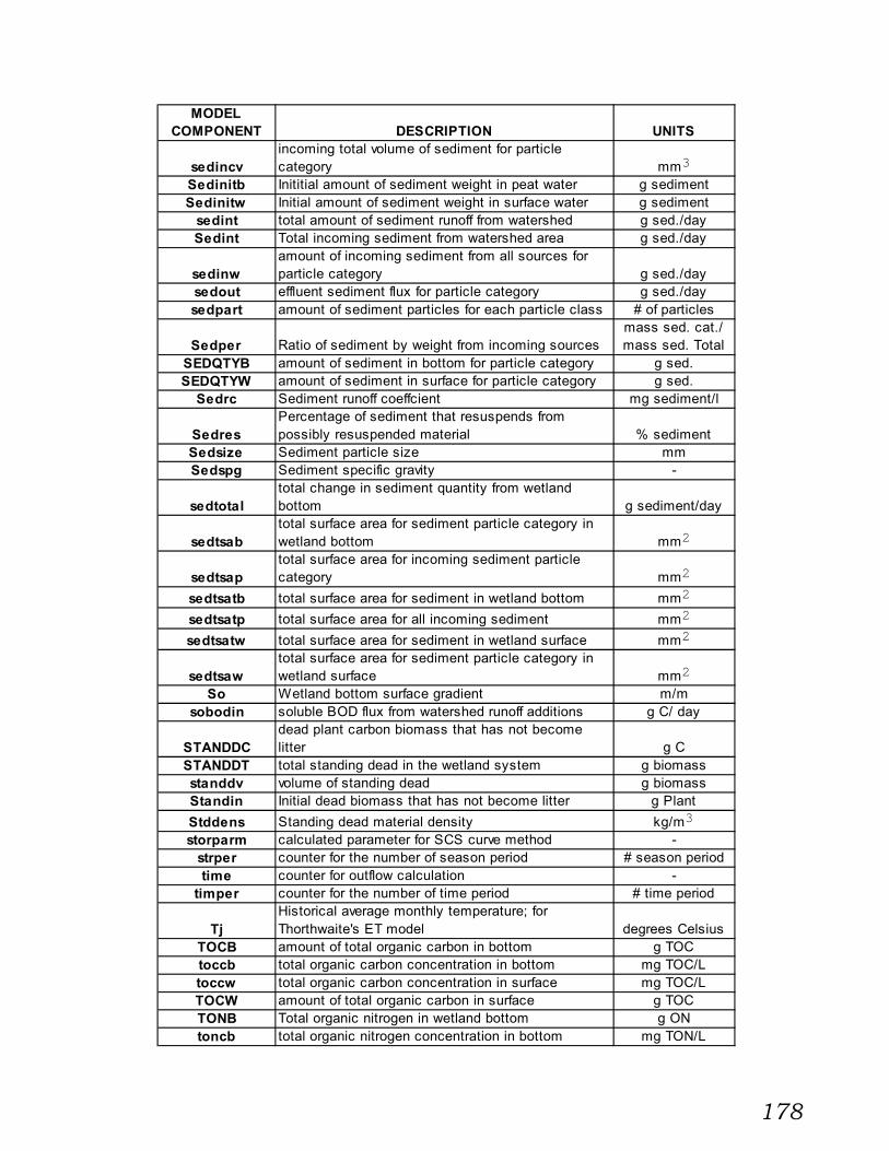
178


sedincvincoming total volume of sediment for particle category mm3

Sedinitb Inititial amount of sediment weight in peat water g sedimentSedinitw Initial amount of sediment weight in surface water g sediment

sedint total amount of sediment runoff from watershed g sed./daySedint Total incoming sediment from watershed area g sed./day

sedinwamount of incoming sediment from all sources for particle category g sed./day

sedout effluent sediment flux for particle category g sed./daysedpart amount of sediment particles for each particle class # of particles

Sedper Ratio of sediment by weight from incoming sourcesmass sed. cat./ mass sed. Total

SEDQTYB amount of sediment in bottom for particle category g sed.SEDQTYW amount of sediment in surface for particle category g sed.

Sedrc Sediment runoff coeffcient mg sediment/l

SedresPercentage of sediment that resuspends from possibly resuspended material % sediment

Sedsize Sediment particle size mmSedspg Sediment specific gravity -

sedtotaltotal change in sediment quantity from wetland bottom g sediment/day

sedtsabtotal surface area for sediment particle category in wetland bottom mm2

sedtsaptotal surface area for incoming sediment particle category mm2

sedtsatb total surface area for sediment in wetland bottom mm2

sedtsatp total surface area for all incoming sediment mm2

sedtsatw total surface area for sediment in wetland surface mm2

sedtsawtotal surface area for sediment particle category in wetland surface mm2

So Wetland bottom surface gradient m/msobodin soluble BOD flux from watershed runoff additions g C/ day

STANDDCdead plant carbon biomass that has not become litter g C

STANDDT total standing dead in the wetland system g biomassstanddv volume of standing dead g biomassStandin Initial dead biomass that has not become litter g Plant

Stddens Standing dead material density kg/m3

storparm calculated parameter for SCS curve method -strper counter for the number of season period # season periodtime counter for outflow calculation -

timper counter for the number of time period # time period

TjHistorical average monthly temperature; for Thorthwaite's ET model degrees Celsius

TOCB amount of total organic carbon in bottom g TOCtoccb total organic carbon concentration in bottom mg TOC/Ltoccw total organic carbon concentration in surface mg TOC/LTOCW amount of total organic carbon in surface g TOCTONB Total organic nitrogen in wetland bottom g ONtoncb total organic nitrogen concentration in bottom mg TON/L

179


toncw total organic nitrogen concentration in surface mg TON/LTONW Total organic nitrogen in wetland surface g ON

Toppump Height of outflow top (outlet=4) mtphosec Total phosphorous effluent concentration mg P/L

Volat Volatilization (0=not included, 1=included) -volatiz conversion of ammonium ion to ammonium gas g N/day

Volatr Volatilization rate day-1

Waddon Wet atmospheric deposition rate for DON mg DON/LWadnh4 Wet atmospheric deposition rate for NH4 mg NH4+-/L

Wadpon Wet atmospheric deposition rate for PON mg PON/LWasno3 Wet atmospheric deposition rate for NO3 mg NO3--/L

WATERB amount of water in wetland bottom water pool m3

watervel wetland surface water velocity m/day

WATERVOL amount of water in wetland surface water pool m3

Watinput water input to system from watershed m3/day

watint Total water additions to wetland m3/day

watintt amount of water additions for hourly time step m3/hourWattemp Influent water temperature degrees CWettype Wetland type (0=FWS, 1=SSF) -Width Average width of wetland cell m

winkcorate at which living biomass degrades once it starts to die -

winter flag for when winter is in progress -

Wtrshdar Watershed area of adjoining area m2

180

Appendix B: Data entry to Model

A procedural listing of when and how to enter all input parameters to the SET-WETmodel. If the input is mandatory for submodel use, parameter names will be listed with noconstraints. If input is optional and dependent on other values, these constraints will be stated.All input values are capitilized. When there are both season and time period inputs, seasonparameters will be explained first, and then time periods. The number of input values dependson the number of season periods and time periods that are declared. M is the season periodnumber and J is the time period number.

BASE submodel:

WETTYPE, HYDTYPE, POINT, NITCYCLE,SEDCYCLE, PCYCLE, EVAP, PERCINF

If HYDTYPE = 0 then,NUMSTPER, LENGTH, WIDTH, HO, HB, HTI, HII, SO

Else if HYDTYPE = 1 then,NUMSTPER, LENGTH, WIDTH, HO, HB, HTI, HII, SO, WTRSHDAR, SCCURVE

End if

If EVAP = 0 then,TJ1, TJ2, TJ3, TJ4, TJ5, TJ6, TJ7, TJ8, TJ9, TJ10, TJ11, TJ12

HYDROLOGIC submodel:-HYDSTR (hydrologic season period)

If M = 1 and WETTYPE = 0 thenNUMTMPER, PORPEAT

Else if M = 1 and WETTYPE = 1 thenNUMTMPER, POROSITY, HYDCONP

End if

If M = 1 then

If PERCINF = 1 thenPERCINFA

End if

OUTLETIf OUTLET = 1 then

HOUT, OUTWIDTH, HOVERElse if OUTLET = 2 then

181

ANGVNOT, DISEFFC, KHCOEF, HOUT,HOVERElse if OUTLET = 3 then

HOUT, AREAPIPE, CONTCElse if OUTLET = 4 then

FLOWOUT, TOPPUMPElse if OUTLET = 5 then

ALPHA, BETA, COEFK, HOUTElse if OUTLET = 6 then

HOUTEnd if

End if

If M>1 thenNUMTMPER, CHECK1, CHECK2

If CHECK1 = 0 thenPORPEAT, HYDCONP, POROSITY

End if

If CHECK2 = 0 thenIf OUTLET = 1 then

HOUT, OUTWIDTH, HOVER, NCONTElse if OUTLET = 2 then

ANGVNOT, DISEFFC, KHCOEF, HOUTElse if OUTLET = 3 then

HOUT, AREAPIPE, CONTCElse if OUTLET = 4 then

FLOWOUT, TOPPUMPElse if OUTLET = 5 then

ALPHA, BETA, COEFK, HOUTElse if OUTLET = 6 then

HOUTEnd if

End ifEnd if

-HYDTM (hydrologic time period)

If HYDTYPE = 0 thenIf EVAP = 0 then

WATINPUT (J), PRECIPR, AIRTEMP, DAYLENElse if EVAP = 1 then

WATINPUT (J), PRECIPR, PANEVAPEnd if

If POINT = 1 then

182

APFLOW (J)End if

Else if HYDTYPE =1 then

If EVAP = 0 thenPRECIPR, AIRTEMP, DAYLEN

Else if EVAP = 1 thenPRECIPR, PANEVAP

End ifEnd if

If POINT = 1 thenAPFLOW (J)

End if

BIOMASS submodel:

-VEGST (biomass season period)

-This is only called if NITCYCLE = 1 or SEDCYCLE =1

If M = 1 and WETTYPE = 0 thenBIOINIT, STANDIN, PEATACRW, PEATACRB, PEATDENS,PRATEUP,BIODENS, STDDENS, PBIOUW, PSTDUW

Else if M = 1 and WETTYPE = 1 thenBIOINIT, STANDIN, PEATACRB, PEATDENS, PRATEUP

End if

If M =1 thenBIOMREML, DAYREML, ABIOREML, BIOMREMD, DAYREMD,ABIOREMD, DAYWINS, DAYWINE, DEGBIO, DAYSDEG

If M>1 thenCHECK 1, CHECK2

If CHECK1 = 0 thenIf WETTYPE = 0 then

PEATACRW, PEATACRB, PRATEUP, BIODENS,STDDENS, PBIOUW, PSTDUW

Else if WETTYPE = 1 thenPEATACRB, PRATEUP

End if

If CHECK2 = 0 then

183

BIOMREML, DAYREML, ABIOREML, BIOMREMD, DAYREMD,ABIOREMD, DAYWINS, DAYWINE, DEGBIO, DAYSDEG

-VEGTM (biomass time period)

BIOMGRR

NCOB cycles:-Encompasses the carbon, bacteria, nitrogen, and dissolved oxygen (DO) cycles-These are called if NITCYCLE = 1

BACTERIA submodel:

-BACSTR (bacteria season period)

If M = 1 and WETTYPE = 0 thenNITROSIW, NITROSIB, NDRATEW, NDRATEB, NDOHSATW, NDOHSATB,

NMAXGRW, NMAXGRB, NNH4HSCW, NNH4HSCBHETEROIW, HETEROIB, AEMAXGRW,AEMAXGRB, ANMAXGRW, ANMAXGRB,HTDRW, HTDRB, HTDOHSCW, HTDOHSCB, HNO3HSCW, HNO3HSCB,HORGHSCW, HORGHSCB

Else if M = 1 and WETTYPE = 1 thenNITROSIB, NDRATEB, NDOHSATB, NMAXGRB, NNH4HSCBHETEROIB, AEMAXGRB, ANMAXGRB, HTDRB, HTDOHSCB, HNO3HSCB,HORGHSCB

End if



NDRATEW, NDRATEB, NDOHSATW, NDOHSATB,NMAXGRW, NMAXGRB, NNH4HSCW, NNH4HSCB

Else if WETTYPE = 1 thenNDRATEB, NDOHSATB, NMAXGRB, NNH4HSCB

End if


AEMAXGRW, AEMAXGRB, ANMAXGRW, ANMAXGRB, HTDRW, HTDRB, HTDOHSCW, HTDOHSCB,

HNO3HSCW, HNO3HSCB, HORGHSCW, HORGHSCB

184

Else if WETTYPE = 1 thenAEMAXGRB, ANMAXGRB, HTDRB,HTDOHSCB, HNO3HSCB, HORGHSCB

Endif

-BACTIME (bacteria time period)

If (WETTYPE=0) thenWATTEMPW, WATTEMPB

Else if (WETTYPE=1) thenWATTEMPB

CARBON submodel:

-CARSTR (carbon season period)

If M = 1 and WETTYPE = 0 thenREFCINIT, DOCINITW, DOCINITB, POCINITW, POCINITB,BIOCCONT, BODCFRAC, BODPFRAC, LEACHR, MICROBEC, PEATCC,POCFALL, POCRES, MANNC, RESTHC, POCSIZE, MTCDOC, POCCOUT

Else if M = 1 and WETTYPE = 1 thenREFCINIT, DOCINITB, POCINITB, BIOCCONT,BODCFRAC, BODPFRAC, LEACHR, MICROBEC, PEATCC

End if

If POINT = 1 thenBODCONC

If PERCINF = 1 thenDOCININC

If HYDTYPE =1 thenBODRC



BIOCCONT, BODCFRAC, BODPFRAC, LEACHR, MICROBEC,PEATCC, POCFALL, POCRES, MANNC, RESTHC, POCSIZE,MTCDOC, POCCOUT

Else if WETTYPE = 1 thenBIOCCONT, BODCFRAC, BODPFRAC,LEACHR, MICROBEC, PEATCC

End if

185

If CHECK2 = 0 thenIf POINT = 1 then

BODCONCIf PERCINF =1 then

DOCININCIf HYDTYPE = 1 then

BODRC

-CARTM (carbon time period)

If HYDTYPE = 0 thenBODINFCO

NITROGEN submodel:

-NITSTR (nitrogen season cycle)

If M = 1 and WETTYPE = 0 thenATDEP, NITFIX, VOLAT,DONINITW, DONINITB, IMMINITW, IMMINITB, NH4INITW, NH4INITB,NO3INITW, NO3INITB, PONINITW, PONINITB, REFNINIT, BIOMCN,

BIOMPN, HTNO3YW, HTNO3YB, MICRONC, NSYIELDW, NSYIELDB, ONPARTF, PEATNC, PONRES, PONFALL, MTCDON, MTCNH4, MTCNO3, PONSIZE, RESTHN, PONCOUT,Else if M = 1 and WETTYPE = 1 then

ATDEP, NITFIX, VOLAT,DONINITB, IMMINITB, NH4INITB, NO3INITB, PONINITB, REFNINIT,BIOMCN, BIOMPN, HTNO3YB, MICRONC, NSYIELDB, ONPARTF, PEATNC

End if

If NITFIX = 1 thenNITFRATE

If VOLAT =1 thenVOLATR

If ATDEP =1 thenDADDON, WADDON, DADPON, WADPON,DADNH4, WADNH4, DADNO3, WADNO3

If POINT = 1 thenDONCONC, PONCONC, NO3CONC, NH4CONC

If PERCINF = 1 thenDONININC, NH4ININC, NO3ININC

If HYDTYPE = 1 thenORGNRC, NH4RC, NO3RC

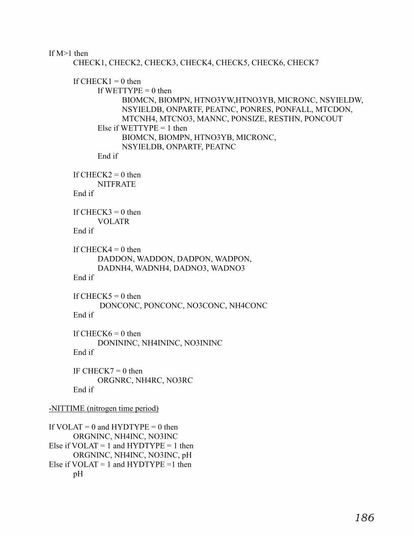
186

If M>1 thenCHECK1, CHECK2, CHECK3, CHECK4, CHECK5, CHECK6, CHECK7


BIOMCN, BIOMPN, HTNO3YW,HTNO3YB, MICRONC, NSYIELDW, NSYIELDB, ONPARTF, PEATNC, PONRES, PONFALL, MTCDON, MTCNH4, MTCNO3, MANNC, PONSIZE, RESTHN, PONCOUT

Else if WETTYPE = 1 thenBIOMCN, BIOMPN, HTNO3YB, MICRONC,NSYIELDB, ONPARTF, PEATNC

End if

If CHECK2 = 0 thenNITFRATE

End if

If CHECK3 = 0 thenVOLATR

End if

If CHECK4 = 0 thenDADDON, WADDON, DADPON, WADPON,DADNH4, WADNH4, DADNO3, WADNO3

End if

If CHECK5 = 0 then DONCONC, PONCONC, NO3CONC, NH4CONC

End if

If CHECK6 = 0 thenDONININC, NH4ININC, NO3ININC

End if

IF CHECK7 = 0 thenORGNRC, NH4RC, NO3RC

End if

-NITTIME (nitrogen time period)

If VOLAT = 0 and HYDTYPE = 0 thenORGNINC, NH4INC, NO3INC

Else if VOLAT = 1 and HYDTYPE = 1 thenORGNINC, NH4INC, NO3INC, pH

Else if VOLAT = 1 and HYDTYPE =1 thenpH

187

End if

DISSOLVED OXYGEN submodel:

-OXYSTR (dissolved oxygen season period)

If M = 1 and WETTYPE = 0 thenDOINITW, DOINITB, HTDOYW, HTDOYB, NSDOYW, NSDOYB,DOCONCP, MTDOX, MTFWSDOC, DOXYCSAT

Else if M = 1 and WETTYPE = 1 thenDOINITB, HTDOYB, NSDOYB, DOCONCP

End if

If POINT = 1 thenOXYCONC

If PERCINF = 1 thenDOININC

If HYDTYPE = 1 thenOXDRC

If M>1 thenCHECK1, CHECK2


HTDOYW, HTDOYB, NSDOYW, NSDOYB, DOCONCP,MTDOX, MTFWSDOC, DOXYCSAT

Else if WETTYPE = 1 thenHTDOYB, NSDOYB, DOCONCP

End if

If CHECK2 = 0 thenIf POINT = 1 then

OXYCONCIf PERCINF = 1 then

DOININCIf HYDTYPE =1 then

OXDRC

-OXYTIME (dissolved oxygen time period)

If HYDTYPE = 0 thenBIOOXRB, DOCONCIN

Else if HYDTYPE =1 thenBIOOXRB

188

End if

SEDIMENT submodel:

-SEDSTR (sediment season period)-Can only be simulated when HYDTYPE = 0

If M = 1 thenSEDCAT, SEDRES

Now depending on the number of sediment categories (SEDCAT)

DO SEDCLASS=1,SEDCATSEDSIZE (SEDCLASS), SEDFALL (SEDCLASS), SEDINITW (SEDCLASS),SEDINITB (SEDCLASS), SEDSPG (SEDCLASS), SEDPER (SEDCLASS)

CONTINUE

If M = 1 thenRESTHICK, MANNC, DECOMPR, PSEDDEP

If POINT =1 thenSEDCONC

If M>1 thenCHECK

IF CHECK = 0 thenRESTHICK, MANNC, DECOMPR

-SEDTIME (sediment time period)

SEDINT

PHOSPHOROUS submodel:

-PHOSSTR (phosphorous season period)-Can only be called if SEDCYCLE =1

M = 1 thenDTPHOSIW, DTPHOSIB, BTPHOSI, PPHOSI, PMINPPC,PRMINBPC, ADSORP, MTCPHOS, BIOMPP

If PERCINF = 1 thenPININC

If ADSORP = 0 thenFREUNDK, FREUNDN

189

Else if ADSORP = 1 or ADSORP = 2 thenLINPARTC

End if

IF POINT =1 or ADSORP =2 thenPHOSCON

If M>1 thenCHECK1, CHECK2

If CHECK1 = 0 thenPMINPPC, PRMINBPC, MTCPHOS, BIOMPP

If PERCINF = 1 thenPININC

End if

If CHECK2 = 0 thenIf ADSORP = 0 then

FREUNDK, FREUNDN, PHOSCONElse if ADSORP = 1 then

LINPARTC, PHOSCONElse if ADSORP =2 then

PHOSCONEnd if

-PHOSTIME (phosphorous time period)

DISPHOSC

If ADSORP = 2 thenPPHOSCAL

190

Appendix C: Model Fortran Code for the SET-WET model

MAIN PROGRAM

PROGRAM WETLANDC MAIN CODE FOR THE SET-WET MODEL (Ver. 1) DEVELOPED BY ERIK LEECC SET-WET IS A CSTR, DYNAMIC, LONG TERM SIMULATION MODEL DESIGNED TO HELPC OPTIMIZE THE CONTROL OF NPS POLLUTION WITH THE USE OF CONSTRUCTEDC WETLANDS. SET-WET MODELS THE HYDROLOGIC, NITROGEN, CARBON, DISSOLVEDC OXYGEN, BACTERIA, VEGTATIVE, SEDIMENT AND PHOSPHOROUS CYCLES OF AC WETLAND.

COMMON /DESCRIBE/ LENGTH,WIDTH,HO,HB,SOREAL WATERVOL(0:500),WATERB(0:500),WATINPUT(0:500),

/ PRECIP(0:500),EVAPT(0:500),HI(0:500),PHYSDEGC(0:500),HT(0:500),SEDSIZE(5), / SEDINITW(5),SEDINITB(5),SEDBV(5), / SEDBSA(5),RESUSP(5,0:500),SEDFALL(5),SEDQTYB(5,0:500), / SEDPER(5,0:500),SEDINW(5,0:500),PHOSPER(5,0:500), / SEDDEP(5,0:500),SEDQTYW(5,0:500),WATINT(0:500), / SEDDELTA(6),DTPHOSW(0:500),BTPHOST(0:500), / OUTFLOW(0:500),HTGROWW(0:500),HTGROWB(0:500),PPHOS(5,0:500), / IMMNB(0:500),NH4CW(0:500),PONCB(0:500),DTPHOSB(0:500), / DONW(0:500),DONB(0:500),PPHOST(0:500),BIOMASST(0:500), / IMMNW(0:500),NH4B(0:500),NO3W(0:500),NO3B(0:500),PONW(0:500), / PONB(0:500),TONCW(0:500),TONCB(0:500),DONOUT(0:500), / REFN(0:500),TONW(0:500),TONB(0:500),DONIN(0:500), / HNH4IMMW(0:500),HNH4IMMB(0:500),DONIMMW(0:500), / DONAMMW(0:500),DONAMMB(0:500),FIXNIT(0:500),DONAT(0:500), / DONDIF(0:500),NH4W(0:500),PONAMMB(0:500),DONIMMB(0:500), / NLEACH(0:500),NITUP(0:500),AMMUP(0:500),DONCW(0:500), / PONIMMW(0:500),PONIMMB(0:500),DEATHB(0:500),IMMNOUT(0:500), / IMMNOUTD(0:500),NH4IN(0:500),DONMINW(0:500),DONMINB(0:500), / PONMINW(0:500),PONMINB(0:500),NH4OUT(0:500),NITRIFW(0:500), / NITRIFB(0:500),NH4DIF(0:500),NH4AT(0:500),VOLATIZ(0:500), / NO3IN(0:500),NO3OUT(0:500),DENITW(0:500),DENITB(0:500), / NO3AT(0:500),NO3DIF(0:500),DEATHW(0:500),PONIN(0:500), / PEATNACW(0:500),PEATNACB(0:500),PONAMMW(0:500),APFLOW(0:500), / PONAT(0:500),PONSET(0:500),PONRE(0:500),DONCB(0:500), / NH4CB(0:500),NO3CW(0:500),NO3CB(0:500),PONCW(0:500), / TOCW(0:500),MICTCNW(0:500),DOCW(0:500),PHOSPERB(5,0:500), / TOCB(0:500),HTDEATHW(0:500),NO3(0:500),ANHTGB(0:500), / MICTCNB(0:500),DOCB(0:500),HTYIELDW(0:500),HTYIELDB(0:500), / BIOMGROW(0:500),NSGROWB(0:500),POCW(0:500),POCB(0:500), / NSDEATHW(0:500),HTDEATHB(0:500),DONIMM(0:500),PON(0:500), / NH4(0:500),NSGROWW(0:500),NH4ATDEP(0:500),ANHTGW(0:500), / PEATACRW(0:500),HETEROW(0:500),NITROSOW(0:500), / ANFRACW(0:500),ANFRACB(0:500),AEROHTGW(0:500),NITROSOB(0:500), / NDEATHW(0:500),NDEATHB(0:500),HETEROB(0:500),AEROHTGB(0:500), / DOCMINIB(0:500),TOCCB(0:500),DOCCB(0:500),DOCMINIW(0:500), / POCMINIB(0:500),PEATCACB(0:500),PEATCACW(0:500),PONOUT(0:500), / POCMINIW(0:500),POCOUT(0:500),DOCOUT(0:500),POCRE(0:500), / BIOMASS(0:500),DOCCW(0:500),POCCW(0:500),POCCB(0:500), / STANDDC(0:500),TOCCW(0:500),REFC(0:500),BIOMDTH(0:500), / BIOMOUT(0:500),SDEADOUT(0:500),STANDDT(0:500), / SOBODIN(0:500),PBODIN(0:500),PHYSDEG(0:500),MICRODW(0:500), / MICRODB(0:500),DOCDIF(0:500),POCSET(0:500),DOCLEACH(0:500), / DOXYW(0:500),DOXYB(0:500),DOINF(0:500),DOOUT(0:500), / DOXYCW(0:500),DOXYCB(0:500),NSRESPW(0:500),NSRESPB(0:500), / DIFOXY(0:500),DIFWS(0:500),HTRESPW(0:500),HTRESPB(0:500), / BTPHOS(5,0:500),SEDPART(5,0:500),PONEC(0:500),SEDSPG(5), / PHOSPERW(5,0:500),NH4EC(0:500),NO3EC(0:500),DONEC(0:500), / SEDOUT(5,0:500),PERCINFT(0:500),BIOMASSV(0:500), / STANDDV(0:500),DTPHOSCW (0:500),DTPHOSCB(0:500), / SEDOUTT(0:500),SEDOUTC(0:500),BOD5CW(0:500),BOD5CB(0:500), / DPHOSOUT(0:500),PPHOSOUT(0:500),DPHOSEC(0:500),TPHOSEC(0:500)

INTEGER NITCYCLE,SEDCYCLE,PCYCLE,NUMSTPER,NUMTMPER,POINT, / STRPER,TIMPER,SEDCAT,SEDCLASS,WETTYPE,EVAP

191

REAL NITROSIW,NITROSIB,DOINITW,DOINITB,POCINITW,POCINITB, / REFCINIT,STANDIN,IMMINITW,IMMINITB,NH4INITW,NH4INITB,HRT, / NO3INITW,NO3INITB,PONINITW,PONINITB,REFNINIT,HETEROIW, / HETEROIB,LENGTH,WIDTH,HO,HB,SO,BIOINIT,PEATACRB,DECOMPR

HYDTYPE=0POINT=0NITCYCLE=0PCYCLE=0SEDCYCLE=0WTRSHDAR=0SCCURVE=0ATDEP=0NITFIX=0VOLAT=0

C OPEN THE MANDATORY UNIT FILES

OPEN (UNIT=2, FILE='base.INP', STATUS='OLD')OPEN (UNIT=3, FILE='hydro.INP', STATUS='OLD')OPEN (UNIT=15, FILE='hydro.OUT', STATUS='OLD')CALL BASE (NUMSTPER,HYDTYPE,NITCYCLE,PCYCLE,SEDCYCLE,

/ WTRSHDAR,SCCURVE,POINT,HEATINDX,EVAPCOEF,HTI,HII,WETTYPE, / EVAP,POROSITY,PERCINF)

IF (NITCYCLE.EQ.1) THENOPEN (UNIT=6, FILE='bac.INP', STATUS='OLD')OPEN (UNIT=8, FILE='nit.INP', STATUS='OLD')OPEN (UNIT=10, FILE='oxy.INP', STATUS='OLD')OPEN (UNIT=12, FILE='car.INP', STATUS='OLD')OPEN (UNIT=16, FILE='bac.OUT', STATUS='OLD')OPEN (UNIT=17, FILE='nit1.OUT', STATUS='OLD')OPEN (UNIT=23, FILE='nit2.OUT',STATUS='OLD')OPEN (UNIT=19, FILE='oxy.OUT', STATUS='OLD')OPEN (UNIT=20, FILE='car1.OUT', STATUS='OLD')OPEN (UNIT=21, FILE='car2.OUT', STATUS='OLD')OPEN (UNIT=24, FILE='bio.INP', STATUS='OLD')OPEN (UNIT=32, FILE='nconc.OUT', STATUS='OLD')

ENDIF

IF (SEDCYCLE.EQ.1 .AND. PCYCLE.EQ.0) THENOPEN (UNIT=9, FILE='sed.INP', STATUS='OLD')OPEN (UNIT=18, FILE='sedw.OUT', STATUS='OLD')OPEN (UNIT=22, FILE='sedb.OUT', STATUS='OLD')

IF (NITCYCLE .EQ. 0) THENOPEN (UNIT=24,FILE='bio.INP',STATUS='OLD')OPEN (UNIT=32, FILE='’nconc.OUT', STATUS='OLD')

ENDIFENDIF

IF (PCYCLE.EQ.1 .AND. SEDCYCLE.EQ.1) THENOPEN (UNIT=9, FILE='sed.INP', STATUS='OLD')OPEN (UNIT=18, FILE='sedw.OUT', STATUS='OLD')OPEN (UNIT=22, FILE='sedb.OUT', STATUS='OLD')OPEN (UNIT=14, FILE='phos.INP', STATUS='OLD')OPEN (UNIT=25, FILE='phos.OUT', STATUS='OLD')

IF (NITCYCLE .EQ. 0) THENOPEN (UNIT=24,FILE='bio.INP',STATUS='OLD')OPEN (UNIT=32, FILE='nconc.OUT', STATUS='OLD')

ENDIF

ELSEIF (PCYCLE.EQ.1 .AND.SEDCYCLE.EQ.0) THENWRITE(*,6)

6 FORMAT ('To model the phosphorous cycle, the ' / 'sediment cycle must also be chosen.'/'Please enter ' / 'a 1 for input SEDCYCLE in the base file or the',/, / 'phosphorous model will not run.',//,' Simulation terminated.')

GO TO 1000ENDIF

192

IF (WETTYPE.EQ.1 .AND. (PCYCLE.EQ.1 .OR. SEDCYCLE.EQ.1)) THENWRITE (*,7)

7 FORMAT ('The sediment cycle and/or phosphorous cycle are ' / 'currently not'/' modeled for SSF wetlands.'//'Please change' / 'data input accordingly, and enter a zero in both '/ / 'SEDCYCLE and PCYCLE in the base file or the model will not ' / 'run properly.'//)

GO TO 1000ENDIF

C START OF SEASON PERIOD LOOP(S)

DO 400 STRPER=1,NUMSTPERM=STRPERCALL HYDSTR(NUMTMPER,POINT,PORPEAT,M,WETTYPE,HYDCONP,

/ POROSITY,PERCINF,PERCINFA)

IF (NITCYCLE.EQ.1. OR. SEDCYCLE.EQ.1) THENCALL VEGST(BIOINIT,BIOMREML,DAYREML,ABIOREML,BIOMREMD,

/ DAYREMD,ABIOREMD,DAYWINS,DEGBIO,DAYSDEG,STANDIN, / PEATACRW,PEATACRB,M,PEATDENS,WETTYPE,PRATEUP,PBIOUW, / BIODENS,STDDENS,PSTDUW,DAYWINE)

ENDIF

IF (NITCYCLE.EQ.1) THENCALL CARSTR (DOCINITW,DOCINITB,POCINITW,POCINITB,

/ POCFALL,POCRES,BIOCCONT,BODCFRAC,MTCDOC,POINT,PERCINF, / BODPFRAC,LEACHR,MICROBEC,PEATCC,BODCONC,HYDTYPE,BODRC, / MANNC,POCSIZE,RESTHC,M,REFCINIT,WETTYPE,POCCOUT,DOCININC)

CALL BACSTR(NITROSIW,NITROSIB,HETEROIW,HETEROIB,M,NDRATEW, / NDRATEB,NDOHSATW,NDOHSATB,NMAXGRW,NMAXGRB,NNH4HSCW,NNH4HSCB, / AEMAXGRW,AEMAXGRB,ANMAXGRW,ANMAXGRB,HTDRW,HTDRB,HTDOHSCW, / HTDOHSCB,HNO3HSCW,HNO3HSCB,HORGHSCW,HORGHSCB,WETTYPE)

CALL NITSTR (POINT,HYDTYPE,MTCDON,NSYIELDB,M,WETTYPE, / NITFRATE,VOLATR,DONCONC,PONCONC,NO3CONC,NH4CONC,MTCNO3, / DONINITW,DONINITB,IMMINITW,IMMINITB,NH4INITW,MTCNH4,HTNO3YB, / NH4INITB,NO3INITW,NO3INITB,PONINITW,PONINITB,REFNINIT,PONCOUT, / BIOMCN,HTNO3YW,MICRONC,NSYIELDW,ONPARTF,PEATNC,BIOMPN,RESTHN, / DADDON,WADDON,DADPON,WADPON,DADNH4,WADNH4,DADNO3,WADNO3, / ORGNRC,NH4RC,NO3RC,PONSIZE,ATDEP,NITFIX,VOLAT,PONRES,PONFALL, / PERCINF,DONININC,NH4ININC,NO3ININC)

CALL OXYSTR (DOINITW,DOINITB,HTDOYB,NSDOYB,HTDOYW, / NSDOYW,DOCONCP,OXYCONC,OXDRC,MTFWSDOC,PERCINF, / MTDOX,POINT,HYDTYPE,M,DOXYCSAT,WETTYPE,DOININC)

ENDIF

IF (SEDCYCLE.EQ.1) THENCALL SEDSTR (SEDSIZE,SEDFALL,SEDINITW,SEDINITB,SEDPER,

/ RESTHICK,SEDBV,SEDBSA,SEDSPG,SEDCAT,MANNC,M,SEDRC, / POINT,SEDCONC,SEDRES,DECOMPR,PSEDDEP) ENDIF

IF (PCYCLE.EQ.1) THENCALL PHOSSTR(DTPHOSIW,PPHOSI,BTPHOSI,M,MTCPHOS,

/ PMINPPC,LINPARTC,FREUNDK,FREUNDN,ADSORP,BIOMPP, / PRMINBPC,POINT,PHOSCON,PHOSRC,DTPHOSIB,PININC,PERCINF)

END IF

C START OF TIME PERIOD LOOP(S)

DO 365 TIMPER=1,NUMTMPERJ=TIMPERK=NUMTMPER

IF (M.EQ.1 .AND. J.EQ.1) THENWRITE (32,*) 'OUTPUT DATA FOR EFFLUENT CONC. IN WETLAND'WRITE(32,275)

193

275 FORMAT (T12,'NH4EC',T23,'NO3EC',T33,'DONEC',T43,'PONEC', / T52,'DOXYCW', t61 'BOD5EC', t71, 'sedoutc', T81, 'DPHOSEC', / T91, 'TPHOSEC')

ENDIF

IF (NITCYCLE.EQ.1 .OR. SEDCYCLE.EQ.1) THENIF (M.EQ.1 .AND. J.EQ.1) THEN

C FROM VEGCYCLEBIOMASST(0)=BIOINITSTANDDT(0)=STANDINBIOMASSV(0)=BIOMASST(0)/1000*(1/BIODENS)STANDDV(0)=STANDDT(0)/1000*(1/STDDENS)

ENDIF

CALL VEGTM(BIOMASST,BIOMREML,DAYREML,ABIOREML,BIOMREMD, / DAYREMD,ABIOREMD,DAYWINS,DEGBIO,DAYSDEG,PHYSDEG, / BIOMGROW,STANDDT,BIOMOUT,BIOMDTH,M,J,K,WETTYPE, / BIODENS,STDDENS,BIOMASSV,STANDDV,DAYWINE)

ENDIF

CALL HYDROT(HYDTYPE,APFLOW,WATERVOL,WATERB,POROSITY, / HEATINDX,EVAPCOEF,HI,HT,WATINPUT,PRECIP,PRECIPR,EVAPT, / OUTFLOW,WATERVEL,HTI,HII,WTRSHDAR,SCCURVE,J,K,M, / PORPEAT,NITCYCLE,SEDCYCLE,WATINT,WETTYPE,EVAP,HYDCONP, / PERCINF,PERCINFA,PERCINFT,BIODENS,STDDENS,PBIOUW, / BIOMASSV,STANDDV,PSTDUW,HRT)

IF(NITCYCLE.EQ.1) THENIF (M.EQ.1 .AND.J.EQ.1) THEN

C OXYGENIF (WETTYPE.EQ.0) THEN

DOXYW(0)=DOINITWDOXYCW(0)=DOXYW(0)/WATERVOL(0)

ENDIFDOXYB(0)=DOINITBDOXYCB(0)=DOXYB(0)/WATERB(0)

C CARBONIF (WETTYPE.EQ.0) THEN

DOCW(0)=DOCINITWDOCCW(0)=DOCW(0)/WATERVOL(0)POCW(0)=POCINITWPOCCW(0)=POCW(0)/WATERVOL(0)TOCW(0)=DOCW(0)+POCW(0)TOCCW(0)=TOCW(0)/WATERVOL(0)

ENDIFDOCB(0)=DOCINITBDOCCB(0)=DOCB(0)/WATERB(0)POCB(0)=POCINITBPOCCB(0)=POCCB(0)/WATERB(0)REFC(0)=REFCINITTOCB(0)=DOCB(0)+POCB(0)TOCCB(0)=TOCB(0)/WATERB(0)BIOMASS(0)=BIOMASST(0)*BIOCCONTSTANDDC(0)=STANDDT(0)*BIOCCONT

C NITROGENIF (WETTYPE.EQ.0)THEN

DONW(0)=DONINITWDONCW(0)=DONW(0)/WATERVOL(0)IMMNW(0)=IMMINITWNH4W(0)=NH4INITWNH4CW(0)=NH4W(0)/WATERVOL(0)NO3W(0)=NO3INITWNO3CW(0)=NO3W(0)/WATERVOL(0)PONW(0)=PONINITWPONCW(0)=PONW(0)/WATERVOL(0)TONW(0)=DONW(0)+PONW(0)

194

TONCW(0)=TONW(0)/WATERVOL(0)ENDIF

DONB(0)=DONINITBDONCB(0)=DONB(0)/WATERB(0)IMMNB(0)=IMMINITBNH4B(0)=NH4INITBNH4CB(0)=NH4B(0)/WATERB(0)NO3B(0)=NO3INITBNO3CB(0)=NO3B(0)/WATERB(0)PONB(0)=PONINITBPONCB(0)=PONB(0)/WATERB(0)REFN(0)=REFNINITTONB(0)=DONB(0)+PONB(0)TONCB(0)=TONB(0)/WATERB(0)

C BACTERIAIF (WETTYPE.EQ.0) THEN

NITROSOW(0)=NITROSIWHETEROW(0)=HETEROIW

ENDIFNITROSOB(0)=NITROSIBHETEROB(0)=HETEROIB

ENDIF

CALL BACTIME (DOXYCW,NSGROWW,HTGROWW,NSGROWB,HTGROWB, / TOCCB,TOCCW,DOXYCB,NH4CW,NH4CB,DOXYW,DOXYB,NO3W,NO3B,NO3CW, / NO3CB,NITROSOW,NITROSOB,HETEROW,HETEROB,NITROSIW,NITROSIB, / HETEROIW,HETEROIB,J,K,M,NDRATEW,NDRATEB,NDOHSATW,ANMAXGRW, / NDOHSATB,NMAXGRW,NMAXGRB,NNH4HSCW,NNH4HSCB,AEMAXGRW, / AEMAXGRB,ANMAXGRB,HTDRW,HTDRB,HTDOHSCW,HTDOHSCB,HNO3HSCW, / HNO3HSCB,HORGHSCW,HORGHSCB,AEROHTGB,AEROHTGW, / NDEATHW,NDEATHB,HTDEATHW,HTDEATHB,WETTYPE,ANHTGW,ANHTGB)

CALL CARTIME(HI,HT,HYDTYPE,BIOMASST,BIOCCONT,BODCFRAC, / BODPFRAC,LEACHR,MICROBEC,PEATCC,REFCINIT,PHYSDEGC,PERCINFT, / POCRES,POCFALL,WATINPUT,HTGROWW,HTGROWB,HTYIELDW,WETTYPE, / HTYIELDB,DONW,DONB,TONW,TONB,DOXYCW,DOXYCB,BIOMASS,DOCININC, / BODRC,DAYSDEG,OUTFLOW,BODCONC,STANDDT,DOCLEACH,MICTCNB, / DOCW,DOCB,POCW,POCB,DOCCW,DOCCB,WATERVOL,WATERB,J,K,M, / POCCW,POCCB,TOCW,TOCB,TOCCW,TOCCB,REFC,STANDDC,MICTCNW, / PEATCACW,PEATCACB,MANNC,RESTHC,POCSIZE,APFLOW,NDEATHW,POCCOUT, / NDEATHB,HTDEATHW,HTDEATHB,PEATACRW,PEATACRB,PONW,PONB,MICDTHW, / MICDTHB,MTCDOC,WATERVEL,DOCINITW,DOCINITB,POCINITW,POCINITB, / PHYSDEG,BIOMDTH,SDEADOUT,POCOUT,DOCOUT)

CALL NITTIME (WATINPUT,PRECIP,OUTFLOW,BIOMGROW,DONW,DONB, / DONCW,DONCB,IMMNW,IMMNB,NH4W,NH4B,NH4CW,NH4CB,NO3W,NO3B, / NO3CW,NO3CB,PONW,PONB,PONCW,PONCB,NO3AT,NO3,MTCNH4, / REFN,TONW,TONB,TONCW,TONCB,BIOMCN,HTNO3YW,MICRONC,BIOMPN, / ONPARTF,PEATNC,DOCLEACH,PHYSDEGC,PONINITB,REFNINIT, / ATDEP,NITFIX,NITFRATE,VOLAT,VOLATR,WATERVOL,WATERB, / PONRES,PONFALL,DONCONC,PONCONC,NO3CONC,J,K,M,HTGROWW,HTGROWB, / NH4CONC,BIOMREML,BIOMREMD,DAYREML,DAYREMD,ABIOREMD, / ABIOREML,MTCDON,HI,HT,HYDTYPE,MANNC,PONSIZE,MTCNO3, / RESTHN,APFLOW,TOCW,MICTCNW,DOCW,TOCB,MICTCNB,DOCB,HTNO3YB, / HTYIELDW,HTYIELDB,NSGROWB,POCW,POCB,HTDEATHW,PEATACRW, / NSDEATHW,HTDEATHB,NSDEATHB,DONIMM,PONIMMW,DONIMMB,PEATACRB, / PON,NSGROWW,NSYIELDW,NSYIELDB,NH4ATDEP,ANHTGW,ANHTGB, / WATERVEL,DADDON,WADDON,DADPON,WADPON,DADNH4,NO3OUT,NH4OUT, / WADNH4,DADNO3,WADNO3,NO3RC,NH4RC,ORGNRC,WETTYPE,DONOUT,PONOUT, / NH4EC,NO3EC,DONEC,PONEC,PONCOUT,PRATEUP,DONININC,NH4ININC, / NO3ININC,PERCINFT)

CALL OXYTIME (DOINITW,DOINITB,HTDOYW,NSDOYW,NSDOYB,OUTFLOW, / NSGROWW,AEROHTGB,J,K,M,NSGROWB,AEROHTGW,WATINPUT,PRECIP, / HTDOYB,DOXYW,DOXYB,OXYCONC,OXDRC,APFLOW,MTFWSDOC, / MTDOX,DOXYCW,DOXYCB,HYDTYPE,HI,HT,WATERVEL,DOCONCP,WATERVOL, / WATERB,DOXYCSAT,WETTYPE,PERCINFT,DOININC,BIOMASST)

ENDIF

195

IF (SEDCYCLE.EQ.1) THENCALL SEDTIME (OUTFLOW,WATERVEL,HT,HI,PHOSPERB,SEDOUTT,

/ RESTHICK,SEDSIZE,SEDFALL,SEDPER,SEDQTYW,SEDQTYB,SEDRES, / MANNC,PHOSPER,J,K,M,SEDRC,WATINPUT,SEDCAT,APFLOW,SEDCONC, / SEDINITW,SEDINITB,SEDBSA,SEDBV,SEDSPG,WATERVOL,DECOMPR, / SEDPART,PHOSPERW,SEDDEP,RESUSP,SEDOUT,PCYCLE,PHYSDEG,PSEDDEP) ENDIF

C INITIAL DETERMINATION OF WATER VOLUME IF NOT AFFECTED BY NUTRIENTC OR SEDIMENT PROCESSESC

IF (NITCYCLE.EQ.0 .AND. SEDCYCLE.EQ.0) THENWATERVOL(J)=WATERVOL(J-1)+WATINT(J)-EVAPT(J)-OUTFLOW(J)-PERCINFT(J)ENDIF

IF (WETTYPE.EQ.0) THENIF (NITCYCLE.EQ.1. .OR. SEDCYCLE.EQ.1) THENCALL DELTAH(DELTAHT,NITCYCLE,SEDCYCLE,SEDTOTAL,SEDDELTA,

/ SEDCAT,SEDSPG,PEATACRB,PEATDENS,HT,NUMTMPER,J,SEDQTYB,WATERB, / PORPEAT)

WATERVOL(J)=WATERVOL(J-1)+WATINT(J)-EVAPT(J) / -OUTFLOW(J)-PERCINFT(J)+(BIOMASSV(J-1)*PBIOUW) / +(STANDDV(J-1)*PSTDUW)-(BIOMASSV(J)*PBIOUW) / -(STANDDV(J)*PSTDUW)-(LENGTH*WIDTH*(HT(J)-HT(J-1)))

ENDIFELSEIF (WETTYPE.EQ.1) THENWATERB(J)=WATERB(J-1)+WATINT(J)-EVAPT(J)-OUTFLOW(J)-PERCINFT(J)ENDIF

C DETERMINATION OF HYDRAULIC RETENTION TIMEC

IF (WETTYPE.EQ.0) THENHRT=WATERVOL(J)/OUTFLOW(J)ELSEIF (WETTYPE.EQ.1) THENHRT=WATERB(J)/OUTFLOW(J)ENDIF

IF (PCYCLE.EQ.1) THENIF (M.EQ.1 .AND. J.EQ.1) THENDTPHOSCW(0)=DTPHOSIW/WATERVOL(0)DTPHOSCB(0)=DTPHOSIB/WATERB(0)ENDIF

CALL PHOSTIME (DTPHOSW,PPHOS,BTPHOS,OUTFLOW,ADSORP,PMINPPC, / FREUNDK,FREUNDN,SEDINITB,SEDINITW,SEDQTYB,SEDQTYW,SEDCAT, / SEDBSA,HI,HT,PPHOST,BTPHOST,SEDINW,APFLOW,PHOSCON, / PHOSPER,BIOMPP,BIOMASST,PHYSDEG,DTPHOSIW,PPHOSI, / WATINPUT,SEDDEP,RESUSP,PRMINBPC,MTCPHOS,BTPHOSI,WATERVOL, / J,K,M,LINPARTC,POINT,PHOSRC,PHOSPERB,DTPHOSIB,DTPHOSB, / WATERB,SEDSPG,SEDBV,PHOSPERW,BIOMGROW,SEDOUT,PRATEUP, / PERCINFT,PININC,DTPHOSCW,DTPHOSCB,DPHOSOUT,PPHOSOUT)

ENDIF

C WRITE VALUES TO OUTPUT FILESC

IF (WETTYPE.EQ.0) THENWRITE(15,75) M,J,WATERVOL(J),WATERB(J),WATINPUT(J),PRECIP(J),

/ WATINT(J),OUTFLOW(J),EVAPT(J),HRT, hi(j), ht(j) 75 FORMAT (T1, (I2), T4, (I3), T7, 6(F9.2, 2X),T73,(F5.1,1X),T81,3(F5.2,2x))

ELSEIF(WETTYPE.EQ.1) THENWRITE(15,100)M,J,WATERB(J),WATINPUT(J),PRECIP(J),WATINT(J),

/ OUTFLOW(J),EVAPT(J),hrt,hi(j),ht(j) 100 FORMAT (T1, (I1), T3, (I3), T7, 6(F9.2, 2X),T73,3(F5.2,1X))

ENDIFIF (HI(J) .GT. HO) THENWRITE(*,101) M,J

101 FORMAT ('THE WETLAND SYSTEM HAS OVERFLOWN THE BANKS AT SEASON' / ' PERIOD ', I2,', TIME PERIOD ', I3)

ENDIFC DETERMINATION OF NUTIENT CONCENTRATIONS

196

CIF (NITCYCLE.EQ.1) THEN

C CARBONIF(WETTYPE.EQ.0) THENDOCCW(J)=DOCW(J)/WATERVOL(J)POCCW(J)=POCW(J)/WATERVOL(J)TOCW(J)=DOCW(J)+POCW(J)TOCCW(J)=TOCW(J)/WATERVOL(J)BOD5CW(J)=((DOCOUT(J)+POCOUT(J))/(1.4*BODCFRAC*OUTFLOW(J)))ENDIFDOCCB(J)=DOCB(J)/WATERB(J)POCCB(J)=POCB(J)/WATERB(J)TOCB(J)=DOCB(J)+POCB(J)TOCCB(J)=TOCB(J)/WATERB(J)BOD5CB(J)=DOCCB(J)/(1.4*BODCFRAC*OUTFLOW(J))

C NITROGENIF (WETTYPE.EQ.0) THENDONCW(J)=DONW(J)/WATERVOL(J)NH4CW(J)=NH4W(J)/WATERVOL(J)NO3CW(J)=NO3W(J)/WATERVOL(J)PONCW(J)=PONW(J)/WATERVOL(J)TONCW(J)=TONW(J)/WATERVOL(J)ENDIFDONCB(J)=DONB(J)/WATERB(J)NH4CB(J)=NH4B(J)/WATERB(J)NO3CB(J)=NO3B(J)/WATERB(J)PONCB(J)=PONB(J)/WATERB(J)TONCB(J)=TONB(J)/WATERB(J)

C OXYGEN/NO BACTERIA NECESSARYIF (WETTYPE.EQ.0) THENDOXYCW(J)=DOXYW(J)/WATERVOL(J)ENDIFDOXYCB(J)=DOXYB(J)/WATERB(J)

ENDIFC SEDIMENT

IF (SEDCYCLE.EQ.1) THENSEDOUTC(J)=SEDOUTT(J)/OUTFLOW(J)

ENDIFC PHOSPHOROUS

IF (PCYCLE.EQ.1) THENDTPHOSCW(J)=DTPHOSW(J)/WATERVOL(J)DTPHOSCB(J)=DTPHOSB(J)/WATERB(J)DPHOSEC(J)=DPHOSOUT(J)/OUTFLOW(J)TPHOSEC(J)=(DPHOSOUT(J)+PPHOSOUT(J))/OUTFLOW(J)

ENDIF

C WRITE TO OUTPUT FILESC BACTERIA

WRITE (16,300) M,J,NITROSOW(J),NITROSOB(J),HETEROW(J),HETEROB(J) 300 FORMAT(T1, (I2),T4,(I3),T8,4(F12.2,3X))C CARBON

WRITE (20,305) M,J,BIOMASS(J),DOCW(J), DOCB(J), POCW(J),POCB(J) 305 FORMAT(T1, (I2),T4,(I3),T8,F11.2,T21,2(F12.2,2X),T50,2(E11.5,2X))

WRITE (21,310) M,J,REFC(J),STANDDC(J),TOCW(J),TOCB(J) 310 FORMAT (T1, (I2),T4,(I3),T8,F11.2,T21,3(F11.2,2X))C NITROGEN

WRITE(17,315) M,J, NO3W(J),NO3B(J),NH4W(J),NH4B(J),IMMNW(J), / IMMNB(J) 315 FORMAT (T1, (I2),T4,(I3),T8,10(F9.1,2X))

WRITE(23 ,320) M,J,DONW(J),DONB(J),PONW(J),PONB(J),REFN(J),TONW(J), / TONB(J),NO3OUT(J) 320 FORMAT (T1, (I2),T4,(I3),T8,8(F9.1,2X))C OXYGEN

WRITE (19,325) M,J,DOXYW(J),DOXYB(J),DOXYCW(J),DOXYCB(J), / DOINF(J),BIOFLUXB,DOOUT(J),HTRESPW(J),HTRESPB(J),NSRESPW(J), / NSRESPB(J),DIFOXY(J),DIFWS(J) 325 FORMAT(T1, (I2),T5,(I3),T9,13(F9.2,2X))C EFFLUENT CONCENTRATIONS

WRITE (32,327) M,J,NH4EC(J),NO3EC(J),DONEC(J),PONEC(J), / doxycw(j),BOD5CW(j),SEDOUTC(J),DPHOSEC(J),TPHOSEC(J)

197

327 FORMAT(T1, (I2),T5,(I3),T9,9(F9.4,1X))C SEDIMENT

IF (SEDCYCLE.EQ.1)THENWRITE(18,330) M,J,SEDQTYW(1,J),SEDQTYW(2,J),SEDQTYW(3,J),

/ SEDQTYW(4,J),SEDQTYW(5,J) 330 FORMAT (T1, (I2), T3, (I3), T8, 5(f11.1, 2X))

WRITE(22,335) M,J,SEDQTYB(1,J),SEDQTYB(2,J),SEDQTYB(3,J), / SEDQTYB(4,J),SEDQTYB(5,J) 335 FORMAT (T1, (I2), T3, (I3), T8, 5(E11.5, 2X))

ENDIFC PHOSPHOROUSC IF (PCYCLE.EQ.1) THEN

WRITE(25,340) M,J,DTPHOSW(J),DTPHOSB(J),BTPHOST(J),PPHOST(J), / DTPHOSCW(J),(PPHOST(J)/WATERVOL(J)) 340 FORMAT(T1, (I2),T5,(I3),T9,4(F10.2,2X),T59,2(F5.2,2X))C ENDIFC 365 CONTINUE

C SET NEW SEASON PERIOD VALUES EQUAL TO END OF PREVIOUS SEASON PERIODC

IF (WETTYPE.EQ.0) THENWATERVOL(0)=WATERVOL(J)

IF (NITCYCLE.EQ.0 .AND. SEDCYCLE.EQ.0) THENWATERB(0)=WATERB(J)

ENDIFHI(0)=HI(J)

ELSEIF (WETTYPE.EQ.1) THENWATERB(0)=WATERB(J)HI(0)=HI(J)

ENDIFC

IF (NITCYCLE.EQ.1 .OR. PCYCLE.EQ.1) THENBIOMASST(0)=BIOMASST(J)STANDDT(0)=STANDDT(J)

ENDIFIF (NITCYCLE.EQ.1) THEN

C BACIF (WETTYPE.EQ.0) THEN

NITROSOW(0)=NITROSOW(J)HETEROW(0)=HETEROW(J)

ENDIFNITROSOB(0)=NITROSOB(J)HETEROB(0)=HETEROB(J)

C CARBONIF (WETTYPE.EQ.0) THEN

DOCW(0)=DOCW(J)POCW(0)=POCW(J)DOCCW(0)=DOCCW(J)POCCW(0)=POCCW(J)TOCW(0)=TOCW(J)TOCCW(0)=TOCCW(J)BOD5CW(0)=BOD5CW(J)

ENDIFDOCB(0)=DOCB(J)POCB(0)=POCB(J)DOCCB(0)=DOCCB(J)POCCB(0)=POCCB(J)TOCB(0)=TOCB(J)TOCCB(0)=TOCCB(J)BOD5CB(0)=BOD5CB(J)REFC(0)=REFC(J)BIOMASS(0)=BIOMASS(J)STANDDC(0)=STANDDC(J)

C OXYGENIF (WETTYPE.EQ.0) THEN

DOXYW(0)=DOXYW(J)DOXYCW(0)=DOXYCW(J)

ENDIFDOXYB(0)=DOXYB(J)

198

DOXYCB(0)=DOXYCB(J)C NITROGEN

IF (WETTYPE.EQ.0) THENDONW(0)=DONW(J)DONCW(0)=DONCW(J)IMMNW(0)=IMMNW(J)NH4W(0)=NH4W(J)NH4CW(0)=NH4CW(J)NO3W(0)=NO3W(J)NO3CW(0)=NO3CW(J)PONW(0)=PONW(J)PONCW(0)=PONCW(J)TONW(0)=TONW(J)TONCW(0)=TONCW(J)

ENDIFDONB(0)=DONB(J)DONCB(0)=DONCB(J)IMMNB(0)=IMMNB(J)NH4B(0)=NH4B(J)NH4CB(0)=NH4CB(J)NO3B(0)=NO3B(J)NO3CB(0)=NO3CB(J)PONB(0)=PONB(J)PONCB(0)=PONCB(J)REFN(0)=REFN(J)TONB(0)=TONB(J)TONCB(0)=TONCB(J)

ENDIFC PHOSPHORUS

IF (PCYCLE.EQ.1) THENDTPHOSCW(0)=DTPHOSCW(J)DTPHOSCB(0)=DTPHOSCB(J)

ENDIF 400 CONTINUE

C SCREEN HELPERSC

IF (NITCYCLE.EQ.1) THENWRITE(*,425)

425 FORMAT ('Nitrogen cycle is included in the simulation.')ELSEIF (NITCYCLE.EQ.0) THENWRITE(*,450)

450 FORMAT ('Nitrogen cycle is not included in the simulation.')ENDIFIF (SEDCYCLE.EQ.1) THENWRITE(*,500)

500 FORMAT (/,'Sediment cycle is included in the simulation.')ELSEIF (SEDCYCLE.EQ.0) THENWRITE(*,600)

600 FORMAT (/,'Sediment cycle is not included in the simulation.') ENDIF

IF (PCYCLE.EQ.1) THENWRITE(*,700)

700 FORMAT (/,'Phosphorous cycle is included in the simulation.',/)ELSEIF (PCYCLE.EQ.0) THENWRITE(*,800)

800 FORMAT (/,'Phosphorous cycle is not included in the ' / 'simulation.',/)

ENDIFC END OF SIMULATION

WRITE (*,900) 900 FORMAT ('Normal termination of simulation.',/)C 1000 END PROGRAM WETLAND

199

BASE SUBMODEL

SUBROUTINE BASE (NUMSTPER,HYDTYPE,NITCYCLE,PCYCLE,SEDCYCLE, / WTRSHDAR,SCCURVE,POINT,HEATINDX,EVAPCOEF,HTI,HII,WETTYPE, / EVAP,POROSITY,PERCINF)

COMMON /DESCRIBE/ LENGTH,WIDTH,HO,HB,SOINTEGER HYDTYPE,POINT,NUMSTPER,NITCYCLE,PCYCLE,SEDCYCLE,WETTYPE,

/ EVAP,PERCINF

REAL LENGTH,WIDTH,HO,HB,HTI,HII,SO,WTRSHDAR, / SCCURVE,TJ,HEATIJ,HEATINDX,EVAPCOEF

HEATINDX=0

C READ IN DESCRIPTION OF WHICH CYCLES AND PROCESSES ARE IN SIMULATIONC

READ(2,*) WETTYPE,HYDTYPE,POINT,NITCYCLE,SEDCYCLE,PCYCLE, / EVAP,PERCINF

C DESCRIPTION OF WETLAND SIZE AND INITIAL WATER LEVELSC

IF (HYDTYPE.EQ.0) THENREAD (2,*) NUMSTPER,LENGTH,WIDTH,HO,HB,HTI,HII,SOENDIFIF (HYDTYPE.EQ.1) THENREAD (2,*) NUMSTPER,LENGTH,WIDTH,HO,HB,HTI,HII,SO,WTRSHDAR,SCCURVEENDIF

IF (EVAP.EQ.0) THENHEATINDX=0

DO 75 KEEP=1,12HEATIJ=0READ(2,*) TJHEATIJ=(TJ/5)**1.514HEATINDX=HEATINDX+HEATIJ

75 CONTINUEEVAPCOEF=6.75E-7*(HEATINDX**3)-7.71E-5*(HEATINDX**2)

/ +1.792E-2*HEATINDX+0.49239ELSE IF (EVAP.EQ.1) THENHEATINDX=0EVAPCOEF=0ENDIF

CEND

200

HYDROLOGIC SUBMODELS

SUBROUTINE HYDSTR(NUMTMPER,POINT,PORPEAT,M,WETTYPE,HYDCONP, / POROSITY,PERCINF,PERCINFA)

COMMON/OUTFLOW/OUTLET,HOUT,OUTWIDTH,HOVER,ANGVNOT,FLOWOUT, / TOPPUMP,AREAPIPE,CONTC,DISEFFC,ALPHA,BETA,COEFK, / KHCOEF

INTEGER POINT,NUMTMPER,CHECK1,CHECK2,OUTLET,WETTYPE,PERCINFREAL HOUT,OUTWIDTH,HOVER,ANGVNOT,HYDCONP,

/ FLOWOUT,TOPPUMP,AREAPIPE,CONTC,DISEFFC,PERCINFA / ALPHA,BETA,COEFK,PORPEAT,KHCOEF,POROSITY

C NUMBER OF TIME PERIODS IN SEASON PERIODC

IF (M.EQ.1) THENIF (WETTYPE.EQ.0) THEN

READ(3,*) NUMTMPER,PORPEATHYDCONP=0.0POROSITY=0

ELSEIF (WETTYPE.EQ.1)THENREAD (3,*) NUMTMPER,POROSITY,HYDCONPPORPEAT=0

ENDIF

IF (PERCINF.EQ.1) THENREAD (3,*) PERCINFA

ELSEIF (PERCINF.EQ.0) THENPERCINFA=0.

ENDIF

HOUT=0.OUTWIDTH=0.HOVER=0.ANGVNOT=0.FLOWOUT=0.TOPPUMP=0.AREAPIPE=0.CONTC=0.DISEFFC=0.ALPHA=0.BEATA=0.COEFK=0.KHCOEF=0.

READ (3,*) OUTLETIF (OUTLET.EQ.1) THEN

READ (3,*) HOUT,OUTWIDTH,HOVERELSEIF (OUTLET.EQ.2)THEN

READ(3,*) ANGVNOT,DISEFFC,KHCOEF,HOUT,HOVERELSEIF (OUTLET.EQ.3) THEN

READ (3,*) HOUT, AREAPIPE, CONTCELSEIF (OUTLET.EQ.4) THEN

READ (3,*) FLOWOUT,TOPPUMPELSEIF (OUTLET.EQ.5) THEN

READ (3,*) ALPHA,BETA,COEFK,HOUTELSEIF (OUTLET.EQ.6)THEN

READ(3,*) HOUTEND IF

ENDIF

C CHECK VALUES TO SEE IF CHANGING BETWEEN SEASON PERIODSC

IF (M.GT.1) THENREAD (3,*) c, NUMTMPER,CHECK1,CHECK2IF (CHECK1.EQ.0) THEN

READ(3,*) PORPEAT,HYDCONP,POROSITYIF (PERCINF.EQ.1) THEN

READ(3,*) PERCINFAENDIF

201

ENDIFIF (CHECK2.EQ.0) THEN

IF (OUTLET.EQ.1) THENREAD(3,*) HOUT,OUTWIDTH,HOVER

ELSEIF (OUTLET.EQ.2) THENREAD(3,*) ANGVNOT,DISEFFC,KHCOEF,HOUT,HOVER

ELSEIF (OUTLET.EQ.3) THENREAD(3,*) HOUT,AREAPIPE,CONTC

ELSEIF (OUTLET.EQ.4) THENREAD(3,*)FLOWOUT,TOPPUMP

ELSEIF (OUTLET.EQ.5) THENREAD(3,*)ALPHA,BETA,COEFK,HOUT

ELSEIF (OUTLET.EQ.6) THENREAD(3,*)HOUT

ENDIFENDIF

ENDIF

ENDCC

SUBROUTINE HYDROT(HYDTYPE,APFLOW,WATERVOL,WATERB,POROSITY, / HEATINDX,EVAPCOEF,HI,HT,WATINPUT,PRECIP,PRECIPR,EVAPT, / OUTFLOW,WATERVEL,HTI,HII,WTRSHDAR,SCCURVE,J,K,M, / PORPEAT,NITCYCLE,SEDCYCLE,WATINT,WETTYPE,EVAP,HYDCONP, / PERCINF,PERCINFA,PERCINFT,BIODENS,STDDENS,PBIOUW, / BIOMASSV,STANDDV,PSTDUW,HRT)

COMMON /DESCRIBE/LENGTH,WIDTH,HO,HB,SOCOMMON/OUTFLOW/OUTLET,HOUT,OUTWIDTH,HOVER,ANGVNOT,FLOWOUT,

/ TOPPUMP,AREAPIPE,CONTC,DISEFFC,ALPHA,BETA,COEFK, / KHCOEF

REAL WATERVOL(0:500),WATERB(0:500),WATINPUT(0:500), / WATINT(0:500),PRECIP(0:500),EVAPT(0:500),OUTFLOW(0:500), / HI(0:500),HT(0:500),HYDCONP,PANEVAP,POROSITY,PERCINFA, / EVAPTT(24),WATINTT(24),OUTFLOWT(24),HIT(0:24),APFLOW(0:500), / PERCINFT(0:500), PERCITT(24),BIOMASSV(0:500),STANDDV(0:500)

INTEGER OUTLET,HYDTYPE,NITCYCLE,SEDCYCLE,WETTYPE,EVAP,TIME, / PERCINF

REAL FT3TOM3,ALPHA,BETA,COEFK,AIRTEMP,DISEFFC / PORPEAT,WTRSHDAR,SCCURVE,HOUT,OUTWIDTH,HOVER,ANGVNOT, / LENGTH,WIDTH,HO,SO,HB,FLOWOUT,TOPPUMP,AREAPIPE,CONTC, / PRECIPR,KHCOEF,M3TOFT3,MTOFT,FTTOM,DAYLEN,HTI,HII, / BIODENS,STDDENS,PBIOUW,PSTDUW,HRT

C INITIAL CONDITIONS OF WATER IN SYSTEMC

IF (J.EQ.1 .AND. M.EQ.1) THENHI(0)=HIIHT(0)=HTIIF (WETTYPE.EQ.0) THENIF (NITCYCLE.EQ.1 .OR. SEDCYCLE.EQ.1) THENWATERVOL(0)=(LENGTH*WIDTH*(HI(0)-HT(0)))

/ -((BIOMASSV(0)*PBIOUW)+(STANDDV(0)*PSTDUW))WATERB(0)=LENGTH*WIDTH*(HT(0)-HB)*PORPEATELSEIF (NITCYCLE.EQ.0 .AND. SEDCYCLE.EQ.0) THENWATERVOL(0)=(LENGTH*WIDTH*(HI(0)-HT(0)))WATERB(0)=LENGTH*WIDTH*(HT(0)-HB)*PORPEATENDIF

C WRITE TO OUTPUT FILESC

WRITE (15,*) 'OUTPUT DATA FOR HYDROLOGIC COUNTS IN WETLAND'WRITE(15,75)

75 FORMAT (T8, 'WATERVOL',T21,'WATERB',T30'WATINPUT',T43,'PRECIP', / T54,'WATINT',T64, 'OUTFLOW',T73, 'EVAPT',T81, 'HRT')

WRITE(15,100) M,WATERVOL(0),WATERB(0) 100 FORMAT (T2, (I1), T4,(' 0 '),T7,2(F9.2,2X))

ELSE IF (WETTYPE.EQ.1) THEN

202

WATERB(0)=LENGTH*WIDTH*(HI(0)-HB)*POROSITYWRITE (15,*) 'OUTPUT DATA FOR HYDROLOGIC COUNTS IN WETLAND'WRITE(15,125)

125 FORMAT (T10, 'WATERB',T19,'WATINPUT',T32'PRECIP',T43,'WATINT', / T53,'OUTFLOW',T66, 'EVAPT',T76, 'HRT')

WRITE(15,150) M,WATERB(0) 150 FORMAT (T1, (I1), T4,(' 0 '),T7,(F9.2,2X))

ENDIFENDIF

IF (NITCYCLE.EQ.0 .AND.SEDCYCLE.EQ.0) THENIF (WETTYPE.EQ.0)THEN

HT(J)=HTI WATERB(J)=LENGTH*WIDTH*(HT(J)-HB)*PORPEATENDIFENDIF

IF (WETTYPE.EQ.1) THENHT(J)=HTI

ENDIF

C READ IN INPUTC

IF (HYDTYPE.EQ.0) THENIF (EVAP.EQ.0) THENREAD (3,*) WATINPUT(J),PRECIPR,AIRTEMP,DAYLENELSEIF (EVAP.EQ.1) THENREAD(3,*)WATINPUT(J),PRECIPR,PANEVAPENDIFIF (POINT.EQ.1) THEN

READ(3,*) APFLOW(J)ELSEIF (POINT.EQ.0) THEN

APFLOW(J)=0ENDIF

PRECIP(J)=PRECIPR*WIDTH*LENGTHWATINT(J)=WATINPUT(J)+PRECIP(J)+APFLOW(J)ENDIF

IF (HYDTYPE.EQ.1) THENIF (EVAP.EQ.0) THENREAD (3,*)PRECIPR,AIRTEMP,DAYLENELSEIF (EVAP.EQ.1) THENREAD(3,*)PRECIPR,PANEVAPENDIF

IF (POINT.EQ.1) THENREAD(3,*) APFLOW(J)

ELSEIF (POINT.EQ.0) THENAPFLOW(J)=0

ENDIF

C DETERMINATION OF HYDROLOGIC INPUT WITH SCS CURVE NUMBER APPROACHC

PRECIP(J)=PRECIPR*WIDTH*LENGTHSTORPARM=25400./SCCURVE-254.FLOWRATE=(((PRECIPR*1000.)-0.2*STORPARM)**2.)/((PRECIPR*1000.)

/ +0.8*STORPARM)WATINPUT(J)=(FLOWRATE/1000.)*(WTRSHDAR-LENGTH*WIDTH)WATINT(J)=WATINPUT(J)+PRECIP(J)+APFLOW(J)ENDIF

C EVAPORATION CALCULATIONSC

IF (EVAP.EQ.0) THENIF(AIRTEMP.LE.0)THEN

EVAPT(J)=0.ELSEIF(AIRTEMP.GT.0) THEN

EVAPT(J)=(1.6*DAYLEN)*((10.*AIRTEMP/HEATINDX)**EVAPCOEF)* / WIDTH*LENGTH/(30.*100.)

203

ENDIFELSEIF (EVAP.EQ.1) THEN

EVAPT(J)=PANEVAP*LENGTH*WIDTHENDIF

C PERCOLATION/INFILTRATION CALCULATIONSC

IF (WETTYPE.EQ.0) THENIF (PERCINF.EQ.0) THEN

PERCINFT(J)=0ELSEIF (PERCINF.EQ.1) THEN

PERCINFT(J)=PERCINFA*LENGTH*WIDTHENDIFELSEIF (WETTYPE.EQ.1) THENIF (PERCINF.EQ.0) THEN

PERCINFT(J)=0ELSEIF (PERCINF.EQ.1) THEN

PERCINFT(J)=PERCINFA*LENGTH*WIDTHENDIFENDIF

C DETERMINATION OF OUTFLOW OVER 24 HOUR TIME FRAMEC

DO 200 TIME=1,24IF (TIME.EQ.1) THEN

HIT(0)=HI(J-1)OUTFLOW(J)=0

ENDIFEVAPTT(TIME)=EVAPT(J)/24WATINTT(TIME)=WATINT(J)/24PERCITT(TIME)=PERCINFT(J)/24

IF (OUTLET.EQ.1) THENIF (HIT(TIME-1).LE.HOUT) THEN

OUTFLOWT(TIME)=0ELSEIF (HIT(TIME-1).GT.HOUT .AND. HIT(TIME-1).LT.HOVER) THEN

OUTFLOWT(TIME)=1.84*(OUTWIDTH-(0.2*(HIT(TIME-1)-HOUT)))* / ((HIT(TIME-1)-HOUT)**1.5)*3600

ELSEIF (HIT(TIME-1).GT.HOVER) THENOUTFLOWT(TIME)=((1.843*(OUTWIDTH-(0.2*(HOVER-HOUT))*

/ ((HOVER-HOUT)**1.5)))+((HIT(TIME-1)-HOVER)*WIDTH))*3600END IF

ELSE IF (OUTLET.EQ.2) THENIF (HIT(TIME-1).LE.HOUT) THEN

OUTFLOWT(TIME)=0ELSEIF (HIT(TIME-1).GT.HOUT) THEN

OUTFLOWT(TIME)=2.363*DISEFFC*(TAN(ANGVNOT/360*22/7))* / (((HIT(TIME-1)-HOUT)+KHCOEF)**(5./2.))*3600

ELSEIF (HIT(TIME-1).GT.HOVER) THENOUTFLOWT(TIME)=(2.363*DISEFFC*(TAN(ANGVNOT/360*22/7))*

/ (((HOVER-HOUT)+KHCOEF)**(5./2.))+(HIT(TIME-1)-HOVER*WIDTH)) / *3600

ENDIFELSE IF (OUTLET.EQ.3) THEN

IF (HIT(TIME-1).LE.HOUT) THENOUTFLOWT(TIME)=0

ELSE IF (HIT(TIME-1).GT.HOUT) THENOUTFLOWT(TIME)=3600*CONTC*AREAPIPE*(SQRT(2.*9.81*

/ (HIT(TIME-1)-HOUT)))ENDIF

ELSE IF (OUTLET.EQ.4) THENIF (HIT(TIME-1).LE.TOPPUMP) THEN

OUTFLOWT(TIME)=0ELSEIF (HIT(TIME-1).GT.TOPPUMP) THEN

OUTFLOWT(TIME)=FLOWOUT/24ENDIF

ELSEIF (OUTLET.EQ.5) THENIF (HIT(TIME-1).LE.HOUT) THEN

WATERVEL=0OUTFLOWT(TIME)=0

204

ELSEIF(HIT(TIME-1).GT.HOUT) THENWATERVEL=COEFK*(((HIT(TIME-1)-HT(J-1))/2)**BETA)*

/ (SO**ALPHA)/((HIT(TIME-1)-HT(J-1))/2)OUTFLOWT(TIME)=WATERVEL*WIDTH*(HIT(TIME-1)-HT(J-1))/24

ENDIFELSE IF (OUTLET.EQ.6) THEN

IF (HIT(TIME-1).GE.HOUT)THENOUTFLOWT(TIME)=MAX(WIDTH*(HIT(TIME-1)-HOUT)*HYDCONP*SO/24,

/ (WATERB(J-1)*HYDCONP/(LENGTH**2*POROSITY)*(WATERB(J-1)/ / (LENGTH*WIDTH*POROSITY)-HOUT)))/24

ELSEIF(HIT(TIME-1).LT.HOUT) THENOUTFLOWT(TIME)=0.0

ENDIFENDIF

IF(WETTYPE.EQ.0) THENHIT(TIME)=HIT(TIME-1)+((WATINTT(TIME)-EVAPTT(TIME)-OUTFLOWT(TIME)

/ -PERCITT(TIME))/(LENGTH*WIDTH))ELSEIF (WETTYPE.EQ.1) THENHIT(TIME)=HIT(TIME-1)+((WATINTT(TIME)-EVAPTT(TIME)-OUTFLOWT(TIME)

/ -PERCITT(TIME))/(LENGTH*WIDTH*POROSITY))ENDIFOUTFLOW(J)=OUTFLOW(J)+OUTFLOWT(TIME)

200 CONTINUE

IF (OUTLET.EQ.1 .OR. OUTLET.EQ.2 .OR. OUTLET.EQ.3 .OR. / OUTLET.EQ.4) THEN

WATERVEL=OUTFLOW(J)/(WIDTH*(HI(J-1)-HT(J-1)))ENDIF

HI(J)=HIT(24)

END

205

VEGETATION SUBMODELS

SUBROUTINE VEGST(BIOINIT,BIOMREML,DAYREML,ABIOREML,BIOMREMD, / DAYREMD,ABIOREMD,DAYWINS,DEGBIO,DAYSDEG,STANDIN, / PEATACRW,PEATACRB,M,PEATDENS,WETTYPE,PRATEUP,PBIOUW, / BIODENS,STDDENS,PSTDUW,DAYWINE)

REAL BIOINIT,ABIOREML,DEGBIO,DAYSDEG,ABIOREMD,REFCINIT,PSTDUW, / STANDIN,PEATACRW,PEATACRB,PEATDENS,STDDENS,BIODENS,PBIOUW

INTEGER BIOMREML,DAYREML,BIOMREMD,DAYREMD,CHECK1,CHECK2, / WETTYPE,DAYWINS,DAYWINE

C READ INITIAL INPUT VALUESC

IF (M.EQ.1) THENIF (WETTYPE.EQ.0) THENREAD (24,*) BIOINIT,STANDIN,PEATACRW,PEATACRB,PEATDENS,

/ PRATEUP,BIODENS,STDDENS,PBIOUW,PSTDUWELSEIF (WETTYPE.EQ.1) THENREAD (24,*) BIOINIT,STANDIN,PEATACRB,PEATDENS,PRATEUPENDIFREAD (24,*) BIOMREML,DAYREML,ABIOREML,BIOMREMD,

/ DAYREMD,ABIOREMD,DAYWINS,DAYWINE,DEGBIO,DAYSDEG ENDIFCC CHECK FOR CHANGES IN PARAMETERS BETWEEN SEASON PERIODSC

IF (M.GT.1) THENREAD(24,*) c, CHECK 1,CHECK2IF (CHECK1.EQ.0) THEN

IF (WETTYPE.EQ.0) THENREAD (24,*) PEATACRW,PEATACRB,PRATEUP,BIODENS,

/ STDDENS,PBIOUW,PSTDUWELSEIF(WETTYPE.EQ.1)THEN

READ(24,*) PEATACRB,PRATEUPENDIF


READ(24,*) BIOMREML,DAYREML,ABIOREML,BIOMREMD,DAYREMD, / ABIOREMD,DAYWINS,DAYWINE,DEGBIO,DAYSDEG

ENDIFENDIFEND

CC

SUBROUTINE VEGTM(BIOMASST,BIOMREML,DAYREML,ABIOREML,BIOMREMD, / DAYREMD,ABIOREMD,DAYWINS,DEGBIO,DAYSDEG,PHYSDEG, / BIOMGROW,STANDDT,BIOMOUT,BIOMDTH,M,J,K,WETTYPE, / BIODENS,STDDENS,BIOMASSV,STANDDV,DAYWINE)

COMMON /DESCRIBE/LENGTH,WIDTH,HO,HB,SOREAL BIOMASST(0:500),BIOMGROW(0:500),BIOMDTH(0:500),

/ SDEADOUT(0:500),PHYSDEG(0:500),STANDDT(0:500),BIOMOUT(0:500), / BIOMASSV(0:500),STANDDV(0:500)

REAL ABIOREML,DEGBIO,DAYSDEG,ABIOREMD,WINKCO, / LENGTH,WIDTH,HO,HB,SO,PRATEUP,BIODENS,STDDENS

INTEGER BIOMREML,DAYREML,BIOMREMD,DAYREMD,WINTER,WETTYPE, / DAYWINS,DAYWINE

PARAMETER (BIODEGR=.012616904)

READ(24,*) BIOMGRR

IF (DAYWINS.EQ.0) THENWINTER=0GO TO 10

ENDIF

IF (J .LT. DAYWINS) THENWINTER=0

ELSE IF ((J .GE. DAYWINS) .AND. (J .LE. DAYWINE)) THEN

206

WINTER=1ELSE IF (J .GT. DAYWINE) THEN

WINTER=0ENDIF

10 IF (WINTER.EQ.0) THENBIOMGROW(J)=LENGTH*WIDTH*BIOMGRRBIOMDTH(J)=0.0

ENDIF

IF (WINTER.EQ.1) THENCC CALCULATION OF EXPONENTIAL DECAYC

WINKCO=-LOG((DEGBIO)/DAYSDEG)BIOMDTH(J)=BIOMASST(J-1)*(EXP(-WINKCO))BIOMGROW(J)=0.0ENDIF

CIF (BIOMREML.EQ.0) THEN

BIOMOUT(J)=0.0ELSE IF (BIOMREML.EQ.1) THEN

IF (J.EQ.DAYREML) THENBIOMOUT(J)=ABIOREML

ELSEBIOMOUT(J)=0.0

ENDIFENDIF

IF (BIOMREMD.EQ.0) THENSDEADOUT(J)=0.0

ELSE IF (BIOMREMD.EQ.1) THENIF (J.EQ.DAYREMD) THEN

SDEADOUT(J)=ABIOREMDELSE

SDEADOUT(J)=0.0ENDIF

ENDIFPHYSDEG(J)=BIODEGR*STANDDT(J-1)

CC TOTAL BIOMASS AND STANDING DEAD MASS BALANCESC

BIOMASST(J)=BIOMASST(J-1)+BIOMGROW(J)-BIOMDTH(J)-BIOMOUT(J)STANDDT(J)=STANDDT(J-1)+BIOMDTH(J)-PHYSDEG(J)-SDEADOUT(J)BIOMASSV(J)=BIOMASST(J)/1000*(1/BIODENS)STANDDV(J)=STANDDT(J)/1000*(1/STDDENS)END

207

CARBON SUBMODELS

SUBROUTINE CARSTR(DOCINITW,DOCINITB,POCINITW,POCINITB, / POCFALL,POCRES,BIOCCONT,BODCFRAC,MTCDOC,POINT,PERCINF, / BODPFRAC,LEACHR,MICROBEC,PEATCC,BODCONC,HYDTYPE,BODRC, / MANNC,POCSIZE,RESTHC,M,REFCINIT,WETTYPE,POCCOUT,DOCININC)

REAL DOCINITW,DOCINITB,POCINITW,POCINITB,REFCINIT, / BIOCCONT,BODCFRAC,BODPFRAC,LEACHR,MICROBEC,MTCDOC, / PEATCC,POCFALL,POCRES,POCCOUT,BODRC / BODCONC,MANNC,RESTHC,POCSIZE,DOCININC

INTEGER CHECK1,CHECK2,HYDTYPE,CHECK3,WETTYPE,POINT,PERCINF

C READ IN INITIAL DATAC

IF (M.EQ.1) THENIF (WETTYPE.EQ.0) THENREAD (12,*) REFCINIT,DOCINITW,DOCINITB,POCINITW,POCINITB,

/ BIOCCONT,BODCFRAC,BODPFRAC,LEACHR,MICROBEC,PEATCC, / POCFALL,POCRES,MANNC,RESTHC,POCSIZE,MTCDOC,POCCOUT

ELSEIF (WETTYPE.EQ.1) THENREAD (12,*) REFCINIT,DOCINITB,POCINITB,BIOCCONT,

/ BODCFRAC,BODPFRAC,LEACHR,MICROBEC,PEATCCENDIF

IF (POINT.EQ.0) THENBODCONC=0.

ELSEIF (POINT.EQ.1) THENREAD (12,*) BODCONC

ENDIF

IF (PERCINF.EQ.0) THENDOCININC=0.0

ELSEIF (PERCINF.EQ.1) THENREAD (12,*) DOCININC

ENDIF

IF (HYDTYPE.EQ.0) THENBODRC=0.0

ELSEIF (HYDTYPE.EQ.1) THENREAD(12,*) BODRC

ENDIFENDIF

C CHECK VALUES TO SEE IF CHANGING BETWEEN SEASON PERIODSC

IF (M.GT.1) THENREAD (12,*) C, CHECK1,CHECK2IF (CHECK1.EQ.0) THEN

IF (WETTYPE.EQ.0)THENREAD (12,*) BIOCCONT,BODCFRAC,BODPFRAC,LEACHR,MICROBEC,

/ PEATCC,POCFALL,POCRES,MANNC,RESTHC,POCSIZE, / MTCDOC,POCCOUT

ELSEIF(WETTYPE.EQ.1) THENREAD (12,*) BIOCCONT,BODCFRAC,BODPFRAC,

/ LEACHR,MICROBEC,PEATCCENDIF


IF (POINT.EQ.1) THENREAD(12,*) BODCONCENDIFIF (PERCINF.EQ.1) THENREAD(12,*) DOCININCENDIFIF(HYDTYPE.EQ.1) THENREAD(12,*) BODRCENDIF

ENDIF

208

ENDIFEND

CSUBROUTINE CARTIME(HI,HT,HYDTYPE,BIOMASST,BIOCCONT,BODCFRAC,

/ BODPFRAC,LEACHR,MICROBEC,PEATCC,REFCINIT,PHYSDEGC,PERCINFT, / POCRES,POCFALL,WATINPUT,HTGROWW,HTGROWB,HTYIELDW,WETTYPE, / HTYIELDB,DONW,DONB,TONW,TONB,DOXYCW,DOXYCB,BIOMASS,DOCININC, / BODRC,DAYSDEG,OUTFLOW,BODCONC,STANDDT,DOCLEACH,MICTCNB, / DOCW,DOCB,POCW,POCB,DOCCW,DOCCB,WATERVOL,WATERB,J,K,M, / POCCW,POCCB,TOCW,TOCB,TOCCW,TOCCB,REFC,STANDDC,MICTCNW, / PEATCACW,PEATCACB,MANNC,RESTHC,POCSIZE,APFLOW,NDEATHW,POCCOUT, / NDEATHB,HTDEATHW,HTDEATHB,PEATACRW,PEATACRB,PONW,PONB,MICDTHW, / MICDTHB,MTCDOC,WATERVEL,DOCINITW,DOCINITB,POCINITW,POCINITB, / PHYSDEG,BIOMDTH,SDEADOUT,POCOUT,DOCOUT)



REAL HTYIELDB(0:500),HTYIELDW(0:500),WATERVOL(0:500), / WATERB(0:500),DOCMINIB(0:500),TOCCB(0:500),DOCCB(0:500), / POCMINIB(0:500),PEATCACB(0:500),PEATCACW(0:500), / DOCMINIW(0:500),BIOMASST(0:500),BIOMASS(0:500),STANDDT(0:500), / POCMINIW(0:500),MICTCNW(0:500),MICTCNB(0:500),DOXYCB(0:500), / POCOUT(0:500),DOCOUT(0:500),POCRE(0:500),DOXYCW(0:500), / DOCW(0:500),DOCCW(0:500),DOCB(0:500),PHYSDEGC(0:500), / POCW(0:500),POCCW(0:500),POCB(0:500),POCCB(0:500),REFC(0:500), / STANDDC(0:500),TOCW(0:500),TOCCW(0:500),TOCB(0:500), / BIOMGROW(0:500),BIOMDTH(0:500), BIOMOUT(0:500),PONB(0:500), / SOBODIN(0:500),PBODIN(0:500),MICRODW(0:500),PERCINFT(0:500), / MICRODB(0:500),DOCMT(0:500),POCSET(0:500),DOCLEACH(0:500), / HI(0:500),HT(0:500),SDEADOUT(0:500),PONW(0:500), / WATINPUT(0:500),OUTFLOW(0:500),TONW(0:500),TONB(0:500), / HTGROWB(0:500),HTGROWW(0:500),DONW(0:500),DONB(0:500), / NDEATHW(0:500),NDEATHB(0:500),HTDEATHW(0:500),HTDEATHB(0:500), / DOCPERC(0:500),APFLOW(0:500), PHYSDEG(0:500)

INTEGER HYDTYPE,WETTYPE,OUTLETC / BIOMREML,DAYREML,WINTER,BIOMREMD,DAYREMD

REAL DOCINITW,DOCINITB,POCINITW,POCINITB,REFCINIT,POCRES, / BIOCCONT,BODCFRAC,BODPFRAC,LEACHR,MICROBEC,WATERVEL, / PEATCC,RESTHC,POCSIZE,LENGTH,WIDTH,HO,HB,SO,MANNC, / ABIOREML,DAYWIN,DEGBIO,POCFALL,BODCONC,ABIOREMD,RESUSPV, / DAYSDEG,MTCDOC,BODRC,PEATACRB,PEATACRW,POCCOUT

C BIODEGREDATION SET AT 95% OVER THE COURSE OF ONE YEARPARAMETER (BIODEGR=.008207485)

C READ IN INPUT VALUESC

IF (HYDTYPE.EQ.0) THENREAD(12,*) BODINFCOENDIF

C DETERMINE HETEROTROPHIC YIELDC

IF(WETTYPE.EQ.0) THENIF (DOXYCW(J-1).EQ.0) THEN

HTYIELDW=.01ELSEIF (DOXYCW(J-1).GE.0 .AND. DOXYCW(J-1).LE.2) THEN

HTYIELDW(J)=DOXYCW(J-1)*.05ELSEIF (DOXYCW(J-1).GT.2. .AND. DOXYCW(J-1).LE.10) THEN

HTYIELDW(J)=.1+((DOXYCW(J-1)-2.)*.1)ELSEIF (DOXYCW(J-1).GT.10.) THEN

HTYIELDW(J)=0.9ENDIFENDIF

IF (DOXYCB(J-1).EQ.0.0) THENHTYIELDB(J)=.01

209

ELSEIF (DOXYCB(J-1).GE.0. .AND. DOXYCB(J-1).LE.2.) THENHTYIELDB(J)=DOXYCB(J-1)*.05

ELSEIF (DOXYCB(J-1).GT.2. .AND. DOXYCB(J-1).LE.10.) THENHTYIELDB(J)=.1+((DOXYCB(J-1)-2.)*.1)

ELSEIF (DOXYCB(J-1).GT.10.) THENHTYIELDB(J)=0.9

ENDIF

C DETERMINE THE MICROBIAL CARBON:NITROGEN RATIOC

IF (WETTYPE.EQ.0) THENIF (DOXYCW(J-1).GE.0. .AND. DOXYCW(J-1).LE.5.) THEN

MICTCNW(J)=80.-10.*DOXYCW(J-1)ELSEIF (DOXYCW(J-1).GE.5.) THEN

MICTCNW(J)=30.ENDIFIF (M.EQ.1 .AND. J. EQ.1) THENMICTCNW(0)=MICTCNW(J)ENDIFENDIF

IF (DOXYCB(J-1).GE.0. .AND. DOXYCB(J-1).LE.5.) THENMICTCNB(J)=80.-10.*DOXYCB(J-1)

ELSEIF (DOXYCB(J-1).GE.5.) THENMICTCNB(J)=30.

ENDIFIF (M.EQ.1 .AND. J.EQ.1) THENMICTCNB(0)=MICTCNB(J)ENDIF

C DOC RELATIONSC

IF (HYDTYPE.EQ.0) THENSOBODIN(J)=1.4*(1-BODPFRAC)*BODCFRAC*(BODINFCO*(WATINPUT(J)+

/ APFLOW(J)*(BODCONC)))ELSEIF (HYDTYPE.EQ.1) THENSOBODIN(J)=1.4*(1-BODPFRAC)*BODCFRAC*(BODRC*WATINPUT(J)+

/ APFLOW(J)*BODCONC)ENDIFDOCLEACH(J)=LENGTH*WIDTH*LEACHRIF(WETTYPE.EQ.0) THENIF (OUTFLOW(J) .LT. WATERVOL(J-1)) THENDOCOUT(J)=DOCW(J-1)*OUTFLOW(J)/(WATERVOL(J-1))ELSEIF (OUTFLOW(J) .GE. WATERVOL (J-1)) THENDOCOUT(J)=.75*DOCW(J-1)*OUTFLOW(J)/WATERVOL(J-1)ENDIFELSEIF (WETTYPE.EQ.1) THENDOCOUT(J)=DOCB(J-1)*OUTFLOW(J)/(WATERB(J-1))ENDIF

IF (WETTYPE.EQ.0) THENIF((TOCW(J-1)/TONW(J-1)).GT.MICTCNW(J-1)) THEN

DOCMINIW(J)=DONW(J-1)/TONW(J-1)*HTGROWW(J)/HTYIELDW(J)ELSE

DOCMINIW(J)=DOCW(J-1)/TOCW(J-1)*HTGROWW(J)/HTYIELDW(J)ENDIFENDIFIF ((TOCB(J-1)/TONB(J-1)).GT.MICTCNB(J-1)) THEN

DOCMINIB(J)=DONB(J-1)/TONB(J-1)*HTGROWB(J)/HTYIELDB(J)ELSE

DOCMINIB(J)=DOCB(J-1)/TOCB(J-1)*HTGROWB(J)/HTYIELDB(J)ENDIF

IF (WETTYPE.EQ.0) THENDOCMT(J)=864*LENGTH*WIDTH*MTCDOC*(DOCCB(J-1)-DOCCW(J-1))ENDIF

IF (PERCINFT(J).GT.0.) THENDOCPERC(J)=DOCB(J-1)*PERCINFT(J)/WATERB(J-1)

ELSEIF (PERCINFT(J).EQ.0.) THEN

210

DOCPERC(J)=0.0ELSEIF (PERCINFT(J).LT.0.) THEN

DOCPERC(J)=PERCINFT(J)*DOCININCENDIF

C MASS BALANCE FOR DOCC

IF (WETTYPE.EQ.0) THENDOCW(J)=DOCW(J-1)+SOBODIN(J)-DOCOUT(J)-DOCMINIW(J)+DOCMT(J)DOCB(J)=DOCB(J-1)-DOCMINIB(J)-DOCMT(J)+DOCLEACH(J)-DOCPERC(J)ELSEIF (WETTYPE.EQ.1) THENDOCB(J)=DOCB(J-1)+SOBODIN(J)+DOCLEACH(J)-DOCOUT(J)

/ -DOCMINIB(J)-DOCPERC(J)ENDIF

C POC RELATIONSC

IF (HYDTYPE.EQ.0) THENPBODIN(J)=1.4*(BODPFRAC)*BODCFRAC*(BODINFCO*WATINPUT(J)+

/ APFLOW(J)*BODCONC)ELSEIF (HYDTYPE.EQ.1) THENPBODIN(J)=1.4*(BODPFRAC)*BODCFRAC*(BODRC*WATINPUT(J)+

/ APFLOW(J)*BODCONC)ENDIF

PHYSDEGC(J)=BIODEGR*STANDDC(J-1)

IF(WETTYPE.EQ.0) THENMICRODW(J)=(NDEATHW(J)+HTDEATHW(J))*MICROBECPEATCACW(J)=PEATACRW*PEATCC

ENDIFMICRODB(J)=(NDEATHB(J)+HTDEATHB(J))*MICROBECPEATCACB(J)=PEATACRB*PEATCC

IF (WETTYPE.EQ.0) THENIF((TOCW(J-1)/TONW(J-1)).GT.MICTCNW(J-1)) THEN

POCMINIW(J)=PONW(J-1)/TONW(J-1)*HTGROWW(J)/HTYIELDW(J)ELSE

POCMINIW(J)=POCW(J-1)/TOCW(J-1)*HTGROWW(J)/HTYIELDW(J)ENDIFENDIFIF ((TOCB(J-1)/TONB(J-1)).GT.MICTCNB(J-1)) THEN

POCMINIB(J)=PONB(J-1)/TONB(J-1)*HTGROWB(J)/HTYIELDB(J)ELSE

POCMINIB(J)=POCB(J-1)/TOCB(J-1)*HTGROWB(J)/HTYIELDB(J)ENDIF

IF (WETTYPE.EQ.0) THENIF (POCFALL.LT.(HI(J-1)-HT(J-1))) THEN

POCSET(J)=POCW(J-1)*(POCFALL)/(HI(J-1)-HT(J-1))ELSE IF (POCFALL.GE.(HI(J-1)-HT(J-1)))THEN

POCSET(J)=POCW(J-1)ENDIF

ENDIF

IF(WETTYPE.EQ.0) THENRESUSPV=7.2*(((POCFALL/86400)**1/3)*

/ ((HI(J-1)-HT(J-1))**(1./6.))/(MANNC*((POCSIZE**(2./3.)))))IF (WATERVEL.GE.RESUSPV) THEN

POCRE(J)=POCB(J-1)*POCRES*RESTHC/(HT(J-1)-HB)ELSE

POCRE(J)=0ENDIFENDIF

IF (WETTYPE.EQ.0) THENIF (OUTLET.EQ.1 .OR. OUTLET.EQ.2. .OR. OUTLET.EQ.3. .OR.

/ OUTLET.EQ.5) THENIF (POCFALL .GT. (HI(J-1)-HT(J-1))) THEN

POCOUT(J)=0.0

211

ELSEIF (POCFALL .LE. (HI(J-1)-HT(J-1)))THENIF (OUTFLOW(J) .LE. WATERVOL(J-1)) THEN

POCOUT(J)=POCCOUT*POCW(J-1)*OUTFLOW(J)/WATERVOL(J-1)ELSEIF (OUTFLOW(J) .GT. WATERVOL(J-1)) THEN

POCOUT(J)=POCCOUT*.5*POCW(J-1)*OUTFLOW(J)/WATERVOL(J-1)ENDIF

ENDIFELSEIF (OUTLET.EQ.4) THENIF (POCFALL .GT. (HI(J-1)-HT(J-1))) THEN

POCOUT(J)=0.ELSEIF (POCFALL .LE. (HI(J-1)-HT(J-1)))THEN

IF (OUTFLOW(J) .LE. WATERVOL(J-1)) THENPOCOUT(J)=((POCW(J-1))*OUTFLOW(J)/WATERVOL(J-1)*POCCOUT)

ELSEIF (OUTFLOW(J) .GT. WATERVOL(J-1)) THENPOCOUT(J)= ((POCW(J-1))*.5*OUTFLOW(J)/WATERVOL(J-1)*POCCOUT)

ENDIFENDIFENDIF

ENDIF

C POC MASS BALANCESC

IF (WETTYPE.EQ.0) THENPOCW(J)=POCW(J-1)+PBODIN(J)+MICRODW(J)-PEATCACW(J)

/ -POCMINIW(J)-POCSET(J)+POCRE(J)-POCOUT(J)+PHYSDEGC(J)POCB(J)=POCB(J-1)+MICRODB(J)-PEATCACB(J)-POCMINIB(J)

/ +POCSET(J)-POCRE(J)ELSEIF (WETTYPE.EQ.1) THENPOCB(J)=POCB(J-1)+PHYSDEGC(J)+PBODIN(J)+MICRODB(J)-PEATCACB(J)

/ -POCMINIB(J)ENDIF

C CARBON BIOMASS/REFRACTORY CARBON/STANDING DEAD CARBONC MASS BALANCEC

BIOMASS(J)=BIOMASS(J-1)+((BIOMASST(J)-BIOMASST(J-1))*BIOCCONT)

IF (WETTYPE.EQ.0) THENREFC(J)=REFC(J-1)+PEATCACW(J)+PEATCACB(J)ELSEIF (WETTYPE.EQ.1) THENREFC(J)=REFC(J-1)+PEATCACB(J)ENDIF

STANDDC(J)=STANDDC(J-1)+((BIOMDTH(J)-PHYSDEG(J)-SDEADOUT(J)) / *BIOCCONT)-DOCLEACH(J)

IF (M.EQ.1 .AND. J.EQ.1) THENWRITE (20,*) 'OUTPUT DATA FOR CARBON COUNTS IN WETLAND'WRITE(20,150)

150 FORMAT(T10,'BIOMASS',T24,'DOCW',T35,'DOCB',T46,'POCW',T57,'POCB')WRITE(20,175) M,BIOMASS(0),DOCW(0),DOCB(0),POCW(0),POCB(0)

175 FORMAT(T1,(I1),T5,(' 0'),T8,F11.2,T21,2(F11.2,2X),t46,2(E11.5,2X)) WRITE (21,*) 'OUTPUT DATA FOR CARBON COUNTS IN WETLAND' WRITE(21,200) 200 FORMAT (T13,'REFC',T23,'STANDDC',T35,'TOCW',T46,'TOCB')

WRITE(21,225) M,REFC(0),STANDDC(0),TOCW(0),TOCB(0) 225 FORMAT (T1, (I2),T5,(' 0'),T8,F11.2,T21,3(F9.2,2X))

ENDIFC

END

212

BACTERIA SUBMODELS

SUBROUTINE BACSTR(NITROSIW,NITROSIB,HETEROIW,HETEROIB,M,NDRATEW, / NDRATEB,NDOHSATW,NDOHSATB,NMAXGRW,NMAXGRB,NNH4HSCW,NNH4HSCB, / AEMAXGRW,AEMAXGRB,ANMAXGRW,ANMAXGRB,HTDRW,HTDRB,HTDOHSCW, / HTDOHSCB,HNO3HSCW,HNO3HSCB,HORGHSCW,HORGHSCB,WETTYPE)

REAL NITROSIW,NITROSIB,NDRATEW,NDRATEB,NDOHSATW,NDOHSATB, / NMAXGRW,NMAXGRB,NNH4HSCW,NNH4HSCB,HETEROIW,HETEROIB, / AEMAXGRB,ANMAXGRW,ANMAXGRB,HTDRW,HTDRB,HTDOHSCW,HTDOHSCB, / HNO3HSCW,HNO3HSCB,HORGHSCW,HORGHSCB,AEMAXGRW

INTEGER CHECK1,CHECK2,WETTYPE,M

C READ IN INITIAL VALUESC

IF (M.EQ.1) THENIF (WETTYPE.EQ.0) THENREAD (6,*) NITROSIW,NITROSIB,NDRATEW,NDRATEB,NDOHSATW,NDOHSATB,

/ NMAXGRW,NMAXGRB,NNH4HSCW,NNH4HSCBREAD(6,*)HETEROIW,HETEROIB,AEMAXGRW,AEMAXGRB,ANMAXGRW,

/ ANMAXGRB,HTDRW,HTDRB,HTDOHSCW,HTDOHSCB,HNO3HSCW,HNO3HSCB, / HORGHSCW,HORGHSCB

ELSEIF (WETTYPE.EQ.1) THENREAD(6,*) NITROSIB,NDRATEB,NDOHSATB,NMAXGRB,NNH4HSCBREAD(6,*) HETEROIB,AEMAXGRB,ANMAXGRB,HTDRB,

/ HTDOHSCB,HNO3HSCB,HORGHSCBENDIFENDIF

C CHECK TO SEE VALUE CHANGES BETWEEN SEASON PERIODSC

IF (M.GT.1) THENREAD (6,*) C, CHECK1,CHECK2IF (CHECK1.EQ.0) THEN

IF (WETTYPE.EQ.0) THENREAD(6,*)NDRATEW,NDRATEB,NDOHSATW,NDOHSATB,

/ NMAXGRW,NMAXGRB,NNH4HSCW,NNH4HSCBELSEIF(WETTYPE.EQ.1) THENREAD(6,*)NDRATEB,NDOHSATB,NMAXGRB,NNH4HSCBENDIF

ENDIF

IF (CHECK2.EQ.0) THENIF (WETTYPE.EQ.0) THENREAD (6,*) AEMAXGRW,AEMAXGRB,ANMAXGRW,ANMAXGRB,

/ HTDRW,HTDRB,HTDOHSCW,HTDOHSCB, / HNO3HSCW,HNO3HSCB,HORGHSCW,HORGHSCB

ELSEIF (WETTYPE.EQ.1) THENREAD (6,*) AEMAXGRB,ANMAXGRB,HTDRB,

/ HTDOHSCB,HNO3HSCB,HORGHSCBENDIF

ENDIFENDIFEND

CC

SUBROUTINE BACTIME (DOXYCW,NSGROWW,HTGROWW,NSGROWB,HTGROWB, / TOCCB,TOCCW,DOXYCB,NH4CW,NH4CB,DOXYW,DOXYB,NO3W,NO3B,NO3CW, / NO3CB,NITROSOW,NITROSOB,HETEROW,HETEROB,NITROSIW,NITROSIB, / HETEROIW,HETEROIB,J,K,M,NDRATEW,NDRATEB,NDOHSATW,ANMAXGRW, / NDOHSATB,NMAXGRW,NMAXGRB,NNH4HSCW,NNH4HSCB,AEMAXGRW,AEMAXGRB, / ANMAXGRB,HTDRW,HTDRB,HTDOHSCW,HTDOHSCB,HNO3HSCW,HNO3HSCB, / HORGHSCW,HORGHSCB,AEROHTGB,AEROHTGW,NDEATHW,NDEATHB,HTDEATHW, / HTDEATHB,WETTYPE,ANHTGW,ANHTGB)

REAL HETEROW(0:500),NITROSOW(0:500),NITROSOB(0:500), / ANFRACW(0:500),ANFRACB(0:500),HTDEATHB(0:500),DOXYCW(0:500), / NSGROWW(0:500),NSGROWB(0:500),AEROHTGW(0:500),ANHTGW(0:500), / HTGROWW(0:500),HTDEATHW(0:500),NDEATHW(0:500),NDEATHB(0:500),

213

/ HETEROB(0:500),AEROHTGB(0:500),ANHTGB(0:500),HTGROWB(0:500), / DOXYCB(0:500),DOXYW(0:500),DOXYB(0:500),NH4CW(0:500), / NH4CB(0:500),TOCCW(0:500),TOCCB(0:500),NO3CW(0:500), / NO3W(0:500),NO3B(0:500),NO3CB(0:500)

REAL NITROSIW,NITROSIB,NDRATEW,NDRATEB,NDOHSATW,NDOHSATB,NMAXGRW, / NMAXGRB,NNH4HSCW,NNH4HSCB,HETEROIW,HETEROIB,AEMAXGRW,AEMAXGRB, / ANMAXGRW,ANMAXGRB,HTDRW,HTDRB,HTDOHSCW,HTDOHSCB,HNO3HSCW, / HNO3HSCB,HORGHSCW,HORGHSCB,WATTEMPW,WATTEMPB,NSTEMPFW, / HTTEMPFW,NSTEMPFB,HTTEMPFB

INTEGER WETTYPE,J,K,M

C READ IN DAILY INPUT VALUESC

IF (WETTYPE.EQ.0) THENREAD(6,*) WATTEMPW,WATTEMPB

ELSEIF (WETTYPE.EQ.1) THENREAD(6,*) WATTEMPB

ENDIF

C BACTERIA TEMPERATURE FACTORC

IF (WETTYPE.EQ.0) THENIF (WATTEMPW.LT.0) THEN

NSTEMPFW=0.HTTEMPFW=0.

ELSEIF (WATTEMPW.GE.0. .AND. WATTEMPW.LE.15.) THENNSTEMPFW=WATTEMPW/15.HTTEMPFW=WATTEMPW/15.

ELSEIF (WATTEMPW.GT.15. .AND. WATTEMPW.LE.35.) THENNSTEMPFW=1.HTTEMPFW=1.

ELSEIF (WATTEMPW.GT.35. .AND. WATTEMPW.LE.40.) THENNSTEMPFW=((40.-WATTEMPW)/5.)HTTEMPFW=((40.-WATTEMPW)/5.)

ELSEIF (WATTEMPW.GT.40.) THENNSTEMPFW=0.0HTTEMPFW=0.0

ENDIFENDIF

IF (WATTEMPB.LT.0) THENNSTEMPFB=0.HTTEMPFB=0.

ELSEIF (WATTEMPB.GE.0. .AND. WATTEMPB.LE.15.) THENNSTEMPFB=WATTEMPB/15.HTTEMPFB=WATTEMPB/15.

ELSEIF (WATTEMPB.GT.15. .AND. WATTEMPB.LE.35.) THENNSTEMPFB=1.HTTEMPFB=1.

ELSEIF (WATTEMPB.GT.35. .AND. WATTEMPB.LE.40.) THENNSTEMPFB=((40.-WATTEMPB)/5.)HTTEMPFB=((40.-WATTEMPB)/5.)

ELSEIF (WATTEMPW.GT.40.) THENNSTEMPFB=0.0HTTEMPFB=0.0

ENDIF

C ANAEROBE FRACTION DETERMINATIONC

IF (WETTYPE.EQ.0) THENIF (DOXYCW(J-1).GE.0. .AND. DOXYCW(J-1).LE.8.) THEN

ANFRACW(J)=0.8-(DOXYCW(J-1)*0.075)ELSEIF (DOXYCW(J-1).GT.8.) THEN

ANFRACW(J)=0.2ENDIFENDIF

IF (DOXYCB(J-1).GE.0. .AND. DOXYCB(J-1).LE.8.) THENANFRACB(J)=0.8-(DOXYCB(J-1)*0.075)

214

ELSEIF (DOXYCB(J-1).GT.8.) THENANFRACB(J)=0.2

ENDIF

C NITROSOMONAS GROWTH AND DEATHC

IF (WETTYPE.EQ.0) THEN NSGROWW(J)=(NMAXGRW*((NH4CW(J-1))/(NNH4HSCW+ / (NH4CW(J-1))))*((DOXYCW(J-1))/(NDOHSATW+(DOXYCW(J-1)))) / *NITROSOW(J-1)*NSTEMPFW)

NDEATHW(J)=NDRATEW*NITROSOW(J-1)ENDIF NSGROWB(J)=(NMAXGRB*((NH4CB(J-1))/

/ (NNH4HSCB+(NH4CB(J-1))))*((DOXYCB(J-1))/(NDOHSATB+ / (DOXYCB(J-1))))*NITROSOB(J-1)*NSTEMPFB)

NDEATHB(J)=NDRATEB*NITROSOB(J-1)

C NITROSOMONAS MASS BALANCEC

IF (WETTYPE.EQ.0) THENNITROSOW(J)=NITROSOW(J-1)+NSGROWW(J)-NDEATHW(J)

ENDIFNITROSOB(J)=NITROSOB(J-1)+NSGROWB(J)-NDEATHB(J)

C HETEROTROPHS GROWTH AND DEATHC

IF (WETTYPE.EQ.0) THENAEROHTGW(J)=(AEMAXGRW*(TOCCW(J-1))/

/ ((TOCCW(J-1))+HORGHSCW)*HTTEMPFW*(DOXYCW(J-1)) / /((DOXYCW(J-1))+HTDOHSCW)*(1-ANFRACW(J))*HETEROW(J-1))

ANHTGW(J)=((ANMAXGRW*TOCCW(J-1))/ / ((TOCCW(J-1))+HORGHSCW)*HTTEMPFW*HTDOHSCW/(HTDOHSCW+ / (DOXYCW(J-1)))*(NO3CW(J-1))/((NO3CW(J-1)) / +HNO3HSCW)*ANFRACW(J)*HETEROW(J-1))

HTGROWW(J)=AEROHTGW(J)+ANHTGW(J)HTDEATHW(J)=HTDRW*HETEROW(J-1)ENDIF

AEROHTGB(J)=(AEMAXGRB*(TOCCB(J-1))/ / ((TOCCB(J-1))+HORGHSCB)*HTTEMPFB*(DOXYCB(J-1))/ / ((DOXYCB(J-1))+HTDOHSCB)*(1-ANFRACB(J))*HETEROB(J-1))

ANHTGB(J)=((ANMAXGRB*TOCCB(J-1))/ / ((TOCCB(J-1))+HORGHSCB)*HTTEMPFB*HTDOHSCB/(HTDOHSCB+ / (DOXYCB(J-1)))*(NO3CB(J-1))/((NO3CB(J-1)) / +HNO3HSCB)*ANFRACB(J)*HETEROB(J-1))

HTGROWB(J)=AEROHTGB(J)+ANHTGB(J)HTDEATHB(J)=HTDRB*HETEROB(J-1)

C MASS BALANCE FOR HETEROTROPHSC

IF (WETTYPE.EQ.0)THENHETEROW(J)=HETEROW(J-1)+HTGROWW(J)-HTDEATHW(J)ENDIFHETEROB(J)=HETEROB(J-1)+HTGROWB(J)-HTDEATHB(J)

C OUTPUT DATAC

IF (M.EQ.1 .AND. J.EQ.1) THENWRITE (16,*) 'OUTPUT DATA FOR BACTERIA COUNTS IN WETLAND'WRITE(16,100)

100 FORMAT (T12,'NITROSOW',T27,'NITROSOB',T43,'HETEROW', / T57,'HETEROB')

WRITE(16,125)M,NITROSOW(0),NITROSOB(0),HETEROW(0),HETEROB(0) 125 FORMAT (T1, (I2),T5,(' 0'),T8,4(F12.2,3X))

ENDIFEND

215

NITROGEN SUBMODELS

SUBROUTINE NITSTR (POINT,HYDTYPE,MTCDON,NSYIELDB,M,WETTYPE, / NITFRATE,VOLATR,DONCONC,PONCONC,NO3CONC,NH4CONC,MTCNO3, / DONINITW,DONINITB,IMMINITW,IMMINITB,NH4INITW,MTCNH4,HTNO3YB, / NH4INITB,NO3INITW,NO3INITB,PONINITW,PONINITB,REFNINIT,PONCOUT, / BIOMCN,HTNO3YW,MICRONC,NSYIELDW,ONPARTF,PEATNC,BIOMPN,RESTHN, / DADDON,WADDON,DADPON,WADPON,DADNH4,WADNH4,DADNO3,WADNO3, / ORGNRC,NH4RC,NO3RC,PONSIZE,ATDEP,NITFIX,VOLAT,PONRES,PONFALL, / PERCINF,DONININC,NH4ININC,NO3ININC)

INTEGER ATDEP,NITFIX,VOLAT,CHECK1,CHECK2,CHECK7 / CHECK3,CHECK4,CHECK5,CHECK6,POINT,WETTYPE,PERCINF

REAL NITFRATE,VOLATR,DONCONC,PONCONC,NO3CONC,NH4CONC, / DONINITW,DONINITB,IMMINITW,IMMINITB,NH4INITW,MTCNH4, / NH4INITB,NO3INITW,NO3INITB,PONINITW,PONINITB,REFNINIT, / BIOMCN,HTNO3YW,MICRONC,NSYIELDW,NSYIELDB,ONPARTF,PEATNC, / DADDON,WADDON,DADPON,WADPON,DADNH4,WADNH4,DADNO3, / WADNO3,ORGNRC,NH4RC,NO3RC,MTCDON,PONSIZE,RESTHN,PONCOUT, / MTCNO3,BIOMPN,PONFALL,HTNO3YB,DONININC,NH4ININC,NO3ININC

IF(M.EQ.1) THEN

C READ IN INITIAL NITROGEN DATAC

IF (WETTYPE.EQ.0) THENREAD (8,*) ATDEP,NITFIX,VOLAT,

/ DONINITW,DONINITB,IMMINITW,IMMINITB,NH4INITW,NH4INITB, / NO3INITW,NO3INITB,PONINITW,PONINITB,REFNINIT,BIOMCN, / BIOMPN,HTNO3YW,HTNO3YB,MICRONC,NSYIELDW,NSYIELDB, / ONPARTF,PEATNC,PONRES,PONFALL,MTCDON,MTCNH4, / MTCNO3,PONSIZE,RESTHN,PONCOUT

ELSEIF(WETTYPE.EQ.1) THENREAD(8,*) ATDEP,NITFIX,VOLAT,

/ DONINITB,IMMINITB,NH4INITB,NO3INITB,PONINITB,REFNINIT, / BIOMCN,BIOMPN,HTNO3YB,MICRONC,NSYIELDB,ONPARTF,PEATNC

ENDIF

C NITROGEN FIXATIONC

IF (NITFIX.EQ.0) THENNITFRATE=0.0

ELSEIF (NITFIX.EQ.1) THENREAD(8,*) NITFRATE

ENDIF

C VOLATILIZATIONC

IF (VOLAT.EQ.0) THENVOLATR=0.0

ELSEREAD(8,*) VOLATR

ENDIF

C ATMOSPHERIC DEPOSITIONC

IF (ATDEP.EQ.0) THENDADDON=0.0WADDON=0.0DADPON=0.0WADPON=0.0DADNH4=0.0WADNH4=0.0DADNO3=0.0WADN03=0.0

ELSEREAD(8,*)DADDON,WADDON,DADPON,WADPON,

/ DADNH4,WADNH4,DADNO3,WADNO3ENDIF

216

C POINT FLOWC

IF (POINT.EQ.1) THENREAD (8,*) DONCONC,PONCONC,NO3CONC,NH4CONC

ELSEDONCONC=0.0PONCONC=0.0NO3CONC=0.0NH4CONC=0.0

ENDIF

C PERCOLATION/INFILITRATIONC

IF (PERCINF.EQ.0) THENDONININC=0.0NH4ININC=0.0NO3ININC=0.0

ELSEIF (PERCINF.EQ.1) THENREAD (8,*) DONININC,NH4ININC,NO3ININC

ENDIF

C INPUT TYPEC

IF (HYDTYPE.EQ.0) THENORGNRC=0.0NH4RC=0.0NO3RC=0.0

ELSEIF (HYDTYPE.EQ.1) THENREAD (8,*) ORGNRC,NH4RC,NO3RC

ENDIFENDIF

C CHECK FOR PARAMETER VALUE CHANGES BETWEEN SEASON PERIODSC

IF (M.GT.1) THENREAD (8,*)c,CHECK1,CHECK2,CHECK3,CHECK4,CHECK5,CHECK6,CHECK7

IF (CHECK1.EQ.0) THENIF (WETTYPE.EQ.0) THENREAD(8,*)BIOMCN,BIOMPN,HTNO3YW,HTNO3YB,MICRONC,NSYIELDW,

/ NSYIELDB,ONPARTF,PEATNC,PONRES,PONFALL,MTCDON, / MTCNH4,MTCNO3,PONSIZE,RESTHN,PONCOUT

ELSEIF(WETTYPE.EQ.1)THENREAD(8,*)BIOMCN,BIOMPN,HTNO3YB,MICRONC,

/ NSYIELDB,ONPARTF,PEATNCENDIF

ENDIF

IF (CHECK2.EQ.0) THENREAD(8,*) NITFRATE


READ(8,*) VOLATRENDIFIF (CHECK4.EQ.0) THEN

READ (8,*) DADDON,WADDON,DADPON,WADPON, / DADNH4,WADNH4,DADNO3,WADNO3


READ (8,*) DONCONC,PONCONC,NO3CONC,NH4CONCENDIFIF (CHECK6.EQ.0) THEN

READ(8,*) DONININC,NH4ININC,NO3ININCENDIFIF (CHECK7.EQ.0) THEN

READ(8,*) ORGNRC,NH4RC,NO3RCENDIFENDIFEND

C

217

CSUBROUTINE NITTIME (WATINPUT,PRECIP,OUTFLOW,BIOMGROW,DONW,DONB,

/ DONCW,DONCB,IMMNW,IMMNB,NH4W,NH4B,NH4CW,NH4CB,NO3W,NO3B, / NO3CW,NO3CB,PONW,PONB,PONCW,PONCB,NO3AT,NO3,MTCNH4, / REFN,TONW,TONB,TONCW,TONCB,BIOMCN,HTNO3YW,MICRONC,BIOMPN, / ONPARTF,PEATNC,DOCLEACH,PHYSDEGC,PONINITB,REFNINIT, / ATDEP,NITFIX,NITFRATE,VOLAT,VOLATR,WATERVOL,WATERB, / PONRES,PONFALL,DONCONC,PONCONC,NO3CONC,J,K,M,HTGROWW,HTGROWB, / NH4CONC,BIOMREML,BIOMREMD,DAYREML,DAYREMD,ABIOREMD, / ABIOREML,MTCDON,HI,HT,HYDTYPE,MANNC,PONSIZE,MTCNO3, / RESTHN,APFLOW,TOCW,MICTCNW,DOCW,TOCB,MICTCNB,DOCB,HTNO3YB, / HTYIELDW,HTYIELDB,NSGROWB,POCW,POCB,HTDEATHW,PEATACRW, / NSDEATHW,HTDEATHB,NSDEATHB,DONIMM,PONIMMW,DONIMMB,PEATACRB, / PON,NSGROWW,NSYIELDW,NSYIELDB,NH4ATDEP,ANHTGW,ANHTGB, / WATERVEL,DADDON,WADDON,DADPON,WADPON,DADNH4,NO3OUT,NH4OUT, / WADNH4,DADNO3,WADNO3,NO3RC,NH4RC,ORGNRC,WETTYPE,DONOUT,PONOUT, / NH4EC,NO3EC,DONEC,PONEC,PONCOUT,PRATEUP,DONININC,NH4ININC, / NO3ININC,PERCINFT)C

REAL OUTFLOW(0:500),HTGROWW(0:500),HTGROWB(0:500), / IMMNB(0:500),NH4CW(0:500),PONCB(0:500),WATERVOL(0:500), / WATERB(0:500),HI(0:500),HT(0:500),DONW(0:500),DONB(0:500), / IMMNW(0:500),NH4B(0:500),NO3W(0:500),NO3B(0:500),PONW(0:500), / PONB(0:500),TONCW(0:500),TONCB(0:500),DONOUT(0:500), / REFN(0:500),TONW(0:500),TONB(0:500),DONIN(0:500), / HNH4IMMW(0:500),HNH4IMMB(0:500),DONIMMW(0:500),DONIMMB(0:500), / DONMINW(0:500),DONMINB(0:500),FIXNIT(0:500),DONAT(0:500), / PRECIP(0:500),WATINPUT(0:500),DONMT(0:500),NH4W(0:500), / NLEACH(0:500),NITUPB(0:500),AMMUPB(0:500),DONCW(0:500), / PONIMMW(0:500),PONIMMB(0:500),DEATHB(0:500),IMMNOUT(0:500), / IMMNOUTD(0:500),NH4IN(0:500),NH4OUT(0:500),NITRIFW(0:500), / NITRIFB(0:500),NH4MT(0:500),NH4AT(0:500),VOLATIZ(0:500), / NO3IN(0:500),NO3OUT(0:500),DENITW(0:500),DENITB(0:500), / NO3AT(0:500),NO3MT(0:500),DEATHW(0:500),PONIN(0:500), / PEATNACW(0:500),PEATNACB(0:500),PONMINW(0:500),PONMINB(0:500), / PONAT(0:500),PONSET(0:500),PONRE(0:500),DONCB(0:500), / NH4CB(0:500),NO3CW(0:500),NO3CB(0:500),PONCW(0:500), / TOCW(0:500),MICTCNW(0:500),DOCW(0:500),NITUPW(0:500), / TOCB(0:500),HTDEATHW(0:500),NO3(0:500),ANHTGB(0:500), / MICTCNB(0:500),DOCB(0:500),HTYIELDW(0:500),HTYIELDB(0:500), / BIOMGROW(0:500),NSGROWB(0:500),POCW(0:500),POCB(0:500), / NSDEATHW(0:500),HTDEATHB(0:500),DONIMM(0:500),PON(0:500), / NSGROWW(0:500),NH4ATDEP(0:500),ANHTGW(0:500),DOCLEACH(0:500), / PEATACW(0:500),PEATACB(0:500),PHYSDEGC(0:500), / NSDEATHB(0:500),PONOUT(0:500),NH4EC(0:500),NO3EC(0:500), / DONEC(0:500),PONEC(0:500),AMMUPW(0:500),APFLOW(0:500), / PERCINFT(0:500),DONPERC(0:500),NH4PERC(0:500),NO3PERC(0:500)

INTEGER NITFIX,ATDEP,VOLAT,DAYREMD,DAYREML,BIOMREML,BIOMREMD, / HYDTYPE,WETTYPE,OUTLET

REAL MTCNH4,NSYIELDW,MTCNO3,NSYIELDB,WATERVEL,NH4RC, / BIOMCN,HTNO3YW,HTNO3YB,MICRONC,ONPARTF,PEATNC,BIOMPN / NITFRATE,VOLATR,PONRES,NO3RC,ORGNRC,DONINITW,DONINITB, / PONFALL,DONCONC,PONCONC,NO3CONC,NH4CONC,REFNINIT, / ABIOREMD,ABIOREML,MTCDON,NO3INITW,NO3INITB,PONINITW,PONINITB, / RESUSPV,MANNC,PONSIZE,RESTHN,DADNH4,WADNH4,DADNO3,WADNO3, / DADDON,WADDON,DADPON,WADPON,NH4INITB,NH4INITW, / LENGTH,WIDTH,HO,HB,SO,ORGNINC,NH4INC,NO3INC, / HOUT,OUTWIDTH,HOVER,ANGVNOT,FLOWOUT,KHCOEF,PONCOUT, / TOPPUMP,AREAPIPE,CONTC,DISEFFC,ALPHA,BETA,COEFK,PRATEUP

COMMON /DESCRIBE/LENGTH,WIDTH,HO,HB,S0COMMON/OUTFLOW/OUTLET,HOUT,OUTWIDTH,HOVER,ANGVNOT,FLOWOUT,


C READ INPUT VALUES FOR DAILY INFLOWC

IF (VOLAT.EQ.0. .AND. HYDTYPE.EQ.0) THENREAD(8,*)ORGNINC,NH4INC,NO3INC

ELSE IF (VOLAT.EQ.1 .AND. HYDTYPE.EQ.0) THEN

218

READ(8,*)ORGNINC,NH4INC,NO3INC,PHELSEIF (VOLAT.EQ.1 .AND. HYDTYPE.EQ.1) THEN

READ (8,*) PHENDIFNLEACH(J)=DOCLEACH(J)/BIOMCN

C DON PROCESSESC

IF (WETTYPE.EQ.0) THENIF (OUTFLOW(J) .LT. WATERVOL(J-1)) THENDONOUT(J)=DONW(J-1)*OUTFLOW(J)/(WATERVOL(J-1))ELSEIF (OUTFLOW(J).GE. WATERVOL(J-1)) THENDONOUT(J)=DONW(J-1)*.75ENDIFELSEIF (WETTYPE.EQ.1) THENDONOUT(J)=DONB(J-1)*OUTFLOW(J)/WATERB(J-1)ENDIFDONEC(J)=DONOUT(J)/OUTFLOW(J)

IF (HYDTYPE.EQ.0) THENDONIN(J)=(1-ONPARTF)*(WATINPUT(J)*ORGNINC+APFLOW(J)*DONCONC)

ELSEIF (HYDTYPE.EQ.1) THENDONIN(J)=(1-ONPARTF)*(WATINPUT(J)*ORGNRC+APFLOW(J)*DONCONC)

ENDIF

IF (WETTYPE.EQ.0)THENHNH4IMMW(J)=MICRONC*HTGROWW(J)*NH4W(J-1)/(TONW(J-1)+NH4W(J-1))ENDIFHNH4IMMB(J)=MICRONC*HTGROWB(J)*NH4B(J-1)/(TONB(J-1)+NH4B(J-1))

IF (WETTYPE.EQ.0) THENIF ((TOCW(J-1)/TONW(J-1)).GT.MICTCNW(J-1)) THEN

DONIMMW(J)=(DONW(J-1)/(TONW(J-1)+NH4W(J-1))*MICRONC*HTGROWW(J))ELSE

DONIMMW(J)=(DOCW(J-1)/TOCW(J-1))*(MICRONC*HTGROWW(J)-HNH4IMMW(J))ENDIF

ENDIFIF ((TOCB(J-1)/TONB(J-1)).GT.MICTCNB(J-1)) THEN

DONIMMB(J)=(DONB(J-1)/(TONB(J-1)+NH4B(J-1))*MICRONC*HTGROWB(J))ELSE

DONIMMB(J)=(DOCB(J-1)/TOCB(J-1))*(MICRONC*HTGROWB(J)-HNH4IMMB(J))ENDIF

IF (WETTYPE.EQ.0) THENIF (((TOCW(J-1)/TONW(J-1)).GT.MICTCNW(J-1)) .OR. (DOCW(J-1).LT.0.1)) THEN

DONMINW(J)=0.0ELSE

DONMINW(J)=(DOCW(J-1)/TOCW(J-1)*HTGROWW(J)/HTYIELDW(J) / *DONW(J-1)/DOCW(J-1)-DONIMMW(J))

IF (DONMINW(J).GE.0) THENDONMINW(J)=DONMINW(J)

ELSEDONMINW(J)=0

ENDIFENDIFENDIF

IF (((TOCB(J-1)/TONB(J-1)).GT.MICTCNB(J-1)) .OR. (DOCB(J-1).LT.0.1)) THENDONMINB(J)=0.0

ELSEDONMINB(J)=(DOCB(J-1)/TOCB(J-1)*HTGROWB(J)/HTYIELDB(J)

/ *DONB(J-1)/DOCB(J-1)-DONIMMB(J))IF(DONMINB(J).LE. 0) THEN

DONMINB(J)=0.0ENDIF

ENDIF

IF (NITFIX.EQ.1) THENFIXNIT(J)=NITFRATE*LENGTH*WIDTH

219

ENDIF

IF (ATDEP.EQ.1) THENIF (PRECIP(J).EQ.0.) THEN

DONAT(J)=DADDON*LENGTH*WIDTHELSE

DONAT(J)=PRECIP(J)*WADDONENDIF

ENDIF

IF (WETTYPE.EQ.0) THENDONMT(J)=864*LENGTH*WIDTH*MTCDON*(DONCB(J-1)-DONCW(J-1))ENDIF

IF (PERCINFT(J).GT.0.) THENDONPERC(J)=DONB(J-1)*PERCINFT(J)/WATERB(J-1)

ELSEIF (PERCINFT(J).EQ.0.) THENDONPERC(J)=0.0

ELSEIF (PERCINFT(J).LT.0.) THENDONPERC(J)=PERCINFT(J)*DONININC

ENDIF

C DON MASS BALANCESC

IF (WETTYPE.EQ.0) THENDONW(J)=DONW(J-1)+DONIN(J)-DONOUT(J)-DONIMMW(J)

/ -DONMINW(J)+FIXNIT(J)+DONAT(J)+DONMT(J)DONB(J)=DONB(J-1)-DONIMMB(J)-DONMINB(J)-DONMT(J)-DONPERC(J)

/ +NLEACH(J)ELSEIF (WETTYPE.EQ.1) THEN

DONB(J)=DONB(J-1)+DONIN(J)+NLEACH(J)-DONOUT(J)-DONIMMB(J)- / DONMINB(J)+FIXNIT(J)+DONAT(J)-DONPERC(J)

ENDIF

C NO3 PROCESSESC

IF (WETTYPE.EQ.0) THENIF (NO3B(J-1).GT.(PRATEUP*BIOMGROW(J)/BIOMPN)) THEN

NITUPB(J)=PRATEUP*BIOMGROW(J)/BIOMPNELSE

NITUPB(J)=NO3B(J-1)ENDIF

IF (NO3W(J-1) .GT. ((1-PRATEUP)*BIOMGROW(J)/BIOMPN)) THENNITUPW(J)=(BIOMGROW(J)*(1-PRATEUP))/BIOMPN

ELSENITUPW(J)=NO3W(J-1)

ENDIFENDIFIF (WETTYPE.EQ.1) THENIF (NO3B(J-1).GT.(BIOMGROW(J)/BIOMPN)) THEN

NITUPB(J)=BIOMGROW(J)/BIOMPNELSE

NITUPB(J)=NO3B(J-1)ENDIFENDIF

C AMMONIUM PROCESSESC

IF (WETTYPE.EQ.0) THENAMMUPW(J)=NSGROWW(J)*MICRONC+(BIOMGROW(J)/BIOMPN*(1-PRATEUP)

/ -(NITUPW(J)))+HNH4IMMW(J)AMMUPB(J)=NSGROWB(J)*MICRONC+((BIOMGROW(J)*PRATEUP/BIOMPN)

/ -(NITUPB(J)))+HNH4IMMB(J)ELSEIF (WETTYPE.EQ.1) THENAMMUPB(J)=NSGROWB(J)*MICRONC+(BIOMGROW(J)/BIOMPN

/ -(NITUPB(J)))+HNH4IMMB(J)ENDIF

220

IF (WETTYPE.EQ.0) THENIF ((TOCW(J-1)/TONW(J-1)).GT.MICTCNW(J-1)) THEN

PONIMMW(J)=PONW(J-1)/(TONW(J-1)+NH4W(J-1))*MICRONC*HTGROWW(J)ELSE

PONIMMW(J)=POCW(J-1)/TOCW(J-1)*(MICRONC*HTGROWW(J)- / (HNH4IMMW(J)))

ENDIF

DEATHW(J)=.2*PHYSDEGC(J)/BIOMCN+MICRONC*(HTDEATHW(J)+NSDEATHW(J))ENDIF

IF ((TOCB(J-1)/TONB(J-1)).GT.MICTCNB(J-1)) THENPONIMMB(J)=PONB(J-1)/(TONB(J-1)+NH4B(J-1))*MICRONC*HTGROWB(J)

ELSEPONIMMB(J)=POCB(J-1)/(TOCB(J-1))*(MICRONC*HTGROWB(J)-

/ (HNH4IMMB(J)))ENDIFDEATHB(J)=.8*PHYSDEGC(J)/BIOMCN+MICRONC*(HTDEATHB(J)+NSDEATHB(J))

CC HERE I AM GOING TO PUT INFORMATION ON THE REMOVAL OF THEC BIOMASS FROM THE SYSTEM WHICH WILL THEN REMOVE A CERTAINC PERCENTAGE OF IMMOBILIZED N THE SYSTEM. WHAT I NEEDC TO FIGURE OUT IS THE AMOUNT THAT NEEDS TO BE REMOVED BASEDC ON THE SEPARATION RATIO BETWEEN THE PLANTS AND MICROBESC BUT WHAT IS THIS SEPARATION

IF (BIOMREML.EQ.0) THENIMMNOUT(J)=0.0

ELSE IF (BIOMREML.EQ.1) THENIF (J.EQ.DAYREML) THEN

IMMNOUT(J)=ABIOREML/BIOMPNELSE

IMMNOUT(J)=0.0ENDIF

ENDIFC

IF (BIOMREMD.EQ.0) THENIMMNOUTD(J)=0.0

ELSE IF (BIOMREMD.EQ.1) THENIF (J.EQ.DAYREMD) THEN

IMMNOUTD(J)=ABIOREMD/BIOMPNELSE

IMMNOUTD(J)=0.0ENDIF

ENDIFC PUT THE RK FOR IMMOBILIZED N HERE

IF (WETTYPE.EQ.0) THENIMMNW(J)=IMMNW(J-1)+DONIMMW(J)+PONIMMW(J)-DEATHW(J)+NITUPW(J)+

/ AMMUPW(J)IMMNB(J)=IMMNB(J-1)+NITUPB(J)+DONIMMB(J)+AMMUPB(J)

/ +PONIMMB(J)-DEATHB(J)-IMMNOUT(J)-IMMNOUTD(J)ELSEIF (WETTYPE.EQ.1) THENIMMNB(J)=IMMNB(J-1)+NITUPB(J)+DONIMMB(J)+AMMUPB(J)+PONIMMB(J)

/ -DEATHB(J)-IMMNOUT(J)-IMMNOUTD(J)ENDIF

C NH4IN=NH4 INFLUENTC PONMINW=PON MINERALIZATION //PONMINBC NH4OUT=NH4 OUTFLOWC AMMUP=ALREADY CALCULATEDC NITRIFW=NITRFICATION RATE //NITRIFB

IF (HYDTYPE.EQ.0) THENNH4IN(J)=(NH4INC*WATINPUT(J))+NH4CONC*APFLOW(J)

ELSEIF (HYDTYPE.EQ.1) THENNH4IN(J)=NH4RC*WATINPUT(J)+NH4CONC*APFLOW(J)

ENDIFC

IF (WETTYPE.EQ.0) THENIF (OUTFLOW(J).LT.WATERVOL(J-1)) THENNH4OUT(J)=NH4W(J-1)/(WATERVOL(J-1))*OUTFLOW(J)ELSEIF (OUTFLOW(J).GE.WATERVOL(J-1)) THENNH4OUT(J)=NH4W(J-1)*.75

221

ENDIFELSEIF (WETTYPE.EQ.1) THENNH4OUT(J)=NH4B(J-1)/WATERB(J-1)*OUTFLOW(J)ENDIFNH4EC(J)=NH4OUT(J)/OUTFLOW(J)IF (WETTYPE.EQ.0) THENNITRIFW(J)=NSGROWW(J)/NSYIELDWENDIFNITRIFB(J)=NSGROWB(J)/NSYIELDB

CC NEED A DIFFUSION EQUATION HERE THE EQUATION SHOULD BASICALLYC GO WITH A DIFFUSION COEFFICIENT AND THEN ID ONE SIDE ISC HIGHER THAN THE OTHER THE GRADIENT GOES IN AC CERTAIN DIRECTION

IF (WETTYPE.EQ.0) THENNH4MT(J)=864*LENGTH*WIDTH*MTCNH4*(NH4CB(J-1)-NH4CW(J-1))

c nh4mt(j)=-.005*nh4w(j-1)ENDIF

CC VOLATILIZATION AND ATDEP WILL BE ADDED HEREC


NH4AT(J)=DADNH4*LENGTH*WIDTHELSE

NH4AT(J)=PRECIP(J)*WADNH4ENDIF

ENDIFIF(VOLAT.EQ.1) THEN

IF (PH.GT.8.) THENC this is form the paper by rao and jessup on the Nflood model

PHDEP=5.8*(10**(PH-10))C VOLATIZ = THE AMOUNT OF VOLATIZATION, PHDEP IS THE PARTITIONINGC BETWEEN NH3 AND NH4+, AND VOLAT C IS A RATE IN

IF (WETTYPE.EQ.0) THENVOLATIZ(J)=VOLATR*PHDEP*NH4W(J-1)ELSEIF (WETTYPE.EQ.1) THENVOLATIZ(J)=VOLATR*PHDEP*NH4B(J-1)ENDIFENDIF

ENDIFC NEED TO HAVE A PH CHECK WHERE IT ONLY COUNTS IF THE PH ISC ABOVE A CERTAIN NUMBER AND PERHAPS A MINIMUM NH3 CONC,C THAT IS NECESSARY FOR THE VOLATILIZATION TO OCCURC

IF (PERCINFT(J).GT.0.) THENNH4PERC(J)=NH4B(J-1)*PERCINFT(J)/WATERB(J-1)

ELSEIF (PERCINFT(J).EQ.0.) THENNH4PERC(J)=0.0

ELSEIF (PERCINFT(J).LT.0.) THENNH4PERC(J)=PERCINFT(J)*NH4ININC

ENDIFC

IF (WETTYPE.EQ.0) THENIF((TOCW(J-1)/TONW(J-1)).GT.MICTCNW(J-1) .OR.

/ (POCW(J-1).LT.0.1)) THENPONMINW(J)=0.0

ELSEPONMINW(J)=POCW(J-1)/TOCW(J-1)*HTGROWW(J)/HTYIELDW(J)

/ *PONW(J-1)/POCW(J-1)- / (POCW(J-1)/TOCW(J-1)*(MICRONC*HTGROWW(J)-HNH4IMMW(J)))

ENDIFENDIFIF((TOCB(J-1)/TONB(J-1)) .GT. MICTCNB(J-1) .OR.

/ (POCB(J-1) .LT. 0.1)) THENPONMINB(J)=0.0

ELSEPONMINB(J)=POCB(J-1)/TOCB(J-1)*HTGROWB(J)/HTYIELDB(J)

/ *PONB(J-1)/POCB(J-1)-

222

/ (POCB(J-1)/TOCB(J-1)*(MICRONC*HTGROWB(J)-HNH4IMMB(J)))IF (PONMINB(J).LE.0) THENPONMINB(J)=0.0ENDIF

ENDIF

C AMMONIUM MASS BALANCEC

IF (WETTYPE.EQ.0) THENNH4W(J)=NH4W(J-1)+NH4IN(J)+DONMINW(J)+PONMINW(J)-NH4OUT(J)

/ -NITRIFW(J)+NH4ATDEP(J)-VOLATIZ(J)+NH4MT(J)-AMMUPW(J)

NH4B(J)=NH4B(J-1)+DONMINB(J)+PONMINB(J)-AMMUPB(J)-NITRIFB(J)-NH4MT(J)

ELSEIF (WETYPE.EQ.1) THENNH4B(J)=NH4B(J-1)+NH4IN(J)+DONMINB(J)+PONMINB(J)-NH4OUT(J)-

/ AMMUPB(J)-NITRIFB(J)+NH4ATDEP(J)-VOLATIZ(J)ENDIF

C NITRATE PROCESSESC

IF (HYDTYPE.EQ.0) THENNO3IN(J)=NO3INC*WATINPUT(J)+NO3CONC*APFLOW(J)

ELSEIF (HYDTYPE.EQ.1)THENNO3IN(J)=NO3RC*WATINPUT(J)+NO3CONC*APFLOW(J)

ENDIF

IF (WETTYPE.EQ.0) THENIF (OUTFLOW(J) .LT. WATERVOL (J-1)) THEN

NO3OUT(J)=NO3W(J-1)/(WATERVOL(J-1))*OUTFLOW(J)ELSEIF (OUTFLOW(J) .GE. WATERVOL (J-1)) THEN

NO3OUT(J)=NO3W(J-1)*.75ENDIFELSEIF (WETTYPE.EQ.1) THEN

NO3OUT(J)=NO3B(J-1)/WATERB(J-1)*OUTFLOW(J)ENDIFNO3EC(J)=NO3OUT(J)/OUTFLOW(J)

IF (WETTYPE.EQ.0) THENDENITW(J)=ANHTGW(J)/HTNO3YW

ENDIFDENITB(J)=ANHTGB(J)/HTNO3YB


NO3AT(J)=DADNO3*LENGTH*WIDTHELSE

NO3AT(J)=PRECIP(J)*WADNO3ENDIF

ENDIF

IF (WETTYPE.EQ.0) THENNO3MT(J)=864*LENGTH*WIDTH*MTCNO3*(NO3CB(J-1)-NO3CW(J-1))ENDIF

IF (PERCINFT(J).GT.0.) THENNO3PERC(J)=NO3B(J-1)*PERCINFT(J)/WATERB(J-1)

ELSEIF (PERCINFT(J).EQ.0.) THENNO3PERC(J)=0.0

ELSEIF (PERCINFT(J).LT.0.) THENNO3PERC(J)=PERCINFT(J)*NO3ININC

ENDIF

C MASS BALANCE FOR NITRATEC

IF(WETTYPE.EQ.0) THENNO3W(J)=NO3W(J-1)+NO3IN(J)+NITRIFW(J)-NO3OUT(J)-DENITW(J)

/ +NO3AT(J)+NO3MT(J)-NITUPW(J)NO3B(J)=NO3B(J-1)+NITRIFB(J)-NITUPB(J)-DENITB(J)-NO3MT(J)--NO3PERC(J)

223

ELSEIF (WETTYPE.EQ.1) THENNO3B(J)=NO3B(J-1)+NO3IN(J)+NITRIFB(J)-NITUPB(J)-NO3OUT(J)-

/ DENITB(J)+NO3AT(J)-NO3PERC(J)ENDIF

C PON PROCESSESC

IF (HYDTYPE.EQ.0) THENPONIN(J)=ONPARTF*(WATINPUT(J)*ORGNINC+APFLOW(J)*PONCONC)

ELSEIF (HYDTYPE.EQ.1) THENPONIN(J)=(ONPARTF)*(WATINPUT(J)*ORGNRC+APFLOW(J)*PONCONC)

ENDIF

IF (WETTYPE.EQ.0) THENPEATNACW(J)=PEATACRW*PEATNCENDIFPEATNACB(J)=PEATACRB*PEATNC


PONAT(J)=DADPON*LENGTH*WIDTHELSE

PONAT(J)=PRECIP(J)*WADPONENDIF

ENDIF

IF (WETTYPE.EQ.0) THENIF(PONFALL.LT.(HI(J-1)-HT(J-1)))THEN

PONSET(J)=PONW(J-1)*(PONFALL)/(HI(J-1)-HT(J-1))ELSEIF (PONFALL.GE.(HI(J-1)-HT(J-1)))THEN

PONSET(J)=PONW(J-1)ENDIF

RESUSPV=7.2*(((PONFALL/86400)**1/3)* / ((HI(J-1)-HT(J-1))**(1./6.))/(MANNC* / ((PONSIZE**(2./3.)))))

IF (WATERVEL.GE.RESUSPV) THENPONRE(J)=PONB(J-1)*PONRES*RESTHN/(HT(J-1)-HB)ELSEPONRE(J)=0ENDIFENDIF

IF (WETTYPE.EQ.0) THENIF (OUTLET.EQ.1 .OR. OUTLET.EQ.2. .OR. OUTLET.EQ.3. .OR.

/ OUTLET.EQ.5) THENIF (PONFALL .GT. (HI(J-1)-HT(J-1))) THENPONOUT(J)=0.0ELSEIF (PONFALL .LT. (HI(J-1)-HT(J-1)))THEN

IF (OUTFLOW(J).LT.WATERVOL(J-1)) THENPONOUT(J)=PONCOUT*((PONW(J-1))*OUTFLOW(J)/WATERVOL(J-1))

ELSEIF (OUTFLOW(J).GE. WATERVOL(J-1)) THENPONOUT(J)=.5*PONCOUT*((PONW(j-1))*OUTFLOW(J)/WATERVOL(J-1))

ENDIFENDIFELSEIF (OUTLET.EQ.4)THENIF (PONFALL .GT. (HI(J-1)-HT(J-1))) THENPONOUT(J)=0.ELSEIF (PONFALL .LT. (HI(J-1)-HT(J-1)))THEN

IF (OUTFLOW(J).LE.WATERVOL(J-1)) THENPONOUT(J)=((PONW(J-1))*OUTFLOW(J)/WATERVOL(J-1)*PONCOUT)

ELSEIF (OUTFLOW(J).GE.WATERVOL(J-1)) THENPONOUT(J)=((PONW(J-1))*.5*OUTFLOW(J-1)/WATERVOL(J-1)*PONCOUT)

ENDIFENDIFENDIF

ENDIFPONEC(J)=PONOUT(J)/OUTFLOW(J)

C MASS BALANCE FOR PON

224

CIF (WETTYPE.EQ.0) THENPONW(J)=PONW(J-1)+DEATHW(J)+PONIN(J)-PEATNACW(J)-PONIMMW(J)

/ -PONMINW(J)-PONSET(J)+PONRE(J)-PONOUT(J)+PONAT(J)PONB(J)=PONB(J-1)+DEATHB(J)-PEATNACB(J)-PONIMMB(J)

/ -PONMINB(J)+PONSET(J)-PONRE(J)ELSEIF (WETTYPE.EQ.1) THENPONB(J)=PONB(J-1)+DEATHB(J)+PONIN(J)-PEATNACB(J)-PONIMMB(J)-

/ PONMINB(J)+PONAT(J)ENDIF

C MASS BALANCE FOR REFRACTORY NC

IF (WETTYPE.EQ.0) THENREFN(J)=REFN(J-1)+PEATNACW(J)+PEATNACB(J)TONW(J)=PONW(J)+DONW(J)TONB(J)=PONB(J)+DONB(J)ELSEIF (WETTYPE.EQ.1) THENREFN(J)=REFN(J-1)+PEATNACB(J)TONB(J)=PONB(J)+DONB(J)ENDIF

C WRITE TO OUTPUT FILESC

IF (J.EQ.1 .AND.M.EQ.1) THENWRITE (17,*) 'OUTPUT DATA FOR NITROGEN COUNTS IN WETLAND'WRITE(17,235)

235 FORMAT (T13,'NO3W',T24,'NO3B',T34,'NH4W',T45,'NH4B',T57 / ,'IMMNW',T68,'IMMNB')

WRITE(17,245) M,NO3W(0),NO3B(0),NH4W(0),NH4B(0),IMMNW(0),IMMNB(0) 245 FORMAT (T1, (I2),T5,(' 0'),T8,6(F9.2,2X))

WRITE(23,*) 'OUTPUT DATA FOR NITROGEN COUNTS IN WETLAND'WRITE(23,255)

255 FORMAT (T13,'DONW',T24,'DONB',T35,'PONW',T46,'PONB',T57 / ,'REFN',T68,'TONW',T79,'TONB')

WRITE(23,265) M,DONW(0),DONB(0),PONW(0),PONB(0),REFN(0),TONW(0), / TONB(0) 265 FORMAT (T1, (I2),T5,(' 0'),T8,7(F9.2,2X))

ENDIFC

END

225

OXYGEN SUBMODELS

SUBROUTINE OXYSTR (DOINITW,DOINITB,HTDOYB,NSDOYB,HTDOYW, / NSDOYW,DOCONCP,OXYCONC,OXDRC,MTFWSDOC,PERCINF, / MTDOX,POINT,HYDTYPE,M,DOXYCSAT,WETTYPE,DOININC)

REAL DOINITW,DOINITB,HTDOYW,NSDOYW,HTDOYB,NSDOYB,DOCONCP, / OXYCONC,OXDRC,MTFWSDOC,MTDOX,DOXYCSAT,DOININC

INTEGER CHECK1,CHECK2,POINT,HYDTYPE,WETTYPE,PERCINF

C READ IN INITIAL INPUT VALUESC

IF (M.EQ.1) THENIF (WETTYPE.EQ.0) THEN

READ (10,*) DOINITW,DOINITB,HTDOYW,HTDOYB,NSDOYW,NSDOYB, / DOCONCP,MTDOX,MTFWSDOC,DOXYCSAT

ELSEIF(WETTYPE.EQ.1) THENREAD(10,*) DOINITB,HTDOYB,NSDOYB,DOCONCPENDIF

IF (POINT.EQ.0) THENOXYCONC=0.

ELSEIF (POINT.EQ.1) THENREAD (10,*) OXYCONC

ENDIF

IF (PERCINF.EQ.0) THENDOININC=0.0

ELSEIF (PERCINF.EQ.1) THENREAD (12,*) DOININC

ENDIF

IF (HYDTYPE.EQ.0 ) THENOXDRC=0.0

ELSEIF (HYDTTYPE.EQ.1) THENREAD(10,*) OXDRC

ENDIFENDIF

CC CHECK FOR VALUE CHANGES BETWEEN SEASON PERIODSC

IF (M.GT.1) THENREAD (10,*)c, CHECK1,CHECK2

IF (CHECK1.EQ.0) THENIF (WETTYPE.EQ.0) THENREAD(10,*)HTDOYW,HTDOYB,NSDOYW,NSDOYB,DOCONCP,

/ MTDOX,MTFWSDOC,DOXYCSATELSEIF (WETTYPE.EQ.1) THENREAD(10,*) HTDOYB,NSDOYB,DOCONCPENDIF

ENDIF

IF (CHECK2.EQ.0) THENIF(POINT.EQ.1) THEN

READ(10,*) OXYCONCENDIFIF (PERCINF.EQ.1) THEN

READ (10,*) DOININCENDIFIF (HYDTYPE.EQ.1) THEN

READ(10,*) OXDRCENDIF

ENDIFENDIF

CEND

CC

226

SUBROUTINE OXYTIME (DOINITW,DOINITB,HTDOYW,NSDOYW,NSDOYB,OUTFLOW, / NSGROWW,AEROHTGB,J,K,M,NSGROWB,AEROHTGW,WATINPUT,PRECIP, / HTDOYB,DOXYW,DOXYB,OXYCONC,OXDRC,APFLOW,MTFWSDOC, / MTDOX,DOXYCW,DOXYCB,HYDTYPE,HI,HT,WATERVEL,DOCONCP,WATERVOL, / WATERB,DOXYCSAT,WETTYPE,PERCINFT,DOININC,BIOMASST)

REAL DOXYW(0:500),DOXYB(0:500),WATERVOL(0:500),WATERB(0:500), / OUTFLOW(0:500),DOINF(0:500),DOOUT(0:500),HI(0:500),HT(0:500), / NSGROWW(0:500),AEROHTGB(0:500),DOXYCW(0:500),DOXYCB(0:500), / NSGROWB(0:500),AEROHTGW(0:500),WATINPUT(0:500),PRECIP(0:500), / NSRESPW(0:500),NSRESPB(0:500),MTDOXY(0:500),MTFWS(0:500), / HTRESPW(0:500),HTRESPB(0:500),DOPERC(0:500),PERCINFT(0:500), / APFLOW(0:500),BIOMASST(0:500)

REAL DOINITW,DOINITB,HTDOYW,NSDOYW,NSDOYB,HTDOYB,OXYCONC,OXDRC, / DOCONCP,MTFWSDOC,MTDOX,LENGTH,WIDTH,HO,SO,HB / WATERVEL,BIOOXRB,BIOFLUXB,DOXYCSAT,DOININC

INTEGER HYDTYPE,WETTYPE,J,K,MCOMMON /DESCRIBE/LENGTH,WIDTH,HO,HB,SO

C READ IN OXYGEN INPUT VALUESC

IF (HYDTYPE.EQ.0) THENREAD (10,*) BIOOXRB,DOCONCINELSEIF (HYDTYPE.EQ.1) THENREAD (10,*) BIOOXRBENDIF

IF (HYDTYPE.EQ.0) THENDOINF(J)=DOCONCIN*WATINPUT(J)+PRECIP(J)*DOCONCP+APFLOW(J)*OXYCONCELSEIF (HYDTYPE.EQ.1) THENDOINF(J)=OXDRC*WATINPUT(J)+APFLOW(J)*OXYCONC+PRECIP(J)*DOCONCPENDIF

BIOFLUXB=BIOOXRB*LENGTH*WIDTH

IF (WETTYPE.EQ.0) THENIF (OUTFLOW(J) .LT. WATERVOL(J-1)) THENDOOUT(J)=DOXYW(J-1)*OUTFLOW(J)/WATERVOL(J-1)ELSEIF (OUTFLOW(J) .GE. WATERVOL (J-1)) THENDOOUT(J)=.75*DOXYW(J-1)*OUTFLOW(J)/WATERVOL(J-1)ENDIFELSEIF (WETTYPE.EQ.1) THENDOOUT(J)=DOXYB(J-1)*OUTFLOW(J)/WATERB(J-1)ENDIF

C MICROBIAL RESPIRATIONC

IF (WETTYPE.EQ.0) THENHTRESPW(J)=AEROHTGW(J)/HTDOYWNSRESPW(J)=NSGROWW(J)/NSDOYWENDIFHTRESPB(J)=AEROHTGB(J)/HTDOYBNSRESPB(J)=NSGROWB(J)/NSDOYB

IF (WETTYPE.EQ.0) THENMTDOXY(J)=864*LENGTH*WIDTH*MTDOX*(DOXYCB(J-1)-DOXYCW(J-1))MTFWS(J)=864*LENGTH*WIDTH*MTFWSDOC*(DOXYCSAT-DOXYCW(J-1))ENDIF

IF (PERCINFT(J).GT.0.) THENDOPERC(J)=DOXYB(J-1)*PERCINFT(J)/WATERB(J-1)

ELSEIF (PERCINFT(J).EQ.0.) THENDOPERC(J)=0.0

ELSEIF (PERCINFT(J).LT.0.) THENDOPERC(J)=PERCINFT(J)*DOININC

ENDIFCC MASS BALANCE FOR DISSOLVED OXYGEN

227

CIF (WETTYPE.EQ.0) THENDOXYW(J)=DOXYW(J-1)+DOINF(J)+MTDOXY(J)+MTFWS(J)-DOOUT(J)

/ -HTRESPW(J)-NSRESPW(J)DOXYB(J)=DOXYB(J-1)+BIOFLUXB-HTRESPB(J)-NSRESPB(J)-MTDOXY(J)

/ -DOPERC(J)ELSEIF (WETTYPE.EQ.1) THENDOXYB(J)=DOXYB(J-1)+DOINF(J)-DOOUT(J)+BIOFLUXB-HTRESPB(J)

/ -NSRESPB(J)-DOPERC(J)ENDIF

CC WRITE TO OUTPUT FILESC

IF (M.EQ.1 .AND.J.EQ.1) THENWRITE (19,*) 'OUTPUT DATA FOR DISSOLVED OXYGEN COUNTS IN WETLAND'WRITE(19,290)

290 FORMAT (T12,'DOXYW',T23,'DOXYB',T33,'DOXYCW',T44,'DOXYCB')WRITE(19,295) M,DOXYW(0),DOXYB(0),DOXYCW(0),DOXYCB(0)

295 FORMAT (T1, (I2),T6,(' 0'),T9,4(F9.2,2X)) ENDIFC

END

228

PHOSPHOROUS SUBMODELS

SUBROUTINE PHOSSTR(DTPHOSIW,PPHOSI,BTPHOSI,M,MTCPHOS, / PMINPPC,LINPARTC,FREUNDK,FREUNDN,ADSORP,BIOMPP, / PRMINBPC,POINT,PHOSCON,PHOSRC,DTPHOSIB,PININC,PERCINF)

INTEGER ADSORP,POINT,CHECK1,CHECK2,PERCINF

REAL DTPHOSI,PPHOSI,BTPHOSI,PMINPPC,PRMINBPC,PHOSCON, / LINPARTC,FREUNDK,FREUNDN,BIOMPP,MTCPHOS,PININC / PHOSRCCC INITIAL INPUT VALUESC

IF (M.EQ.1) THENREAD(14,*) DTPHOSIW,DTPHOSIB,BTPHOSI,PPHOSI,PMINPPC,

/ PRMINBPC,ADSORP,MTCPHOS,BIOMPP

IF (PERCINF.EQ.0) THENPININC=0.0

ELSEIF (PERCINF.EQ.1) THENREAD (10,*) PININC

ENDIF

IF (ADSORP.EQ.0) THENREAD (14,*) FREUNDK,FREUNDNLINPARTC=0.

ELSEIF (ADSORP.EQ.1) THENREAD(14,*) LINPARTCFREUNDK=0.FREUNDN=0.

ELSEIF (ADSORP.EQ.2) THENFREUNDK=0FREUNDN=0READ(14,*) LINPARTC

ENDIF

IF (POINT.EQ.1 .OR. ADSORP.EQ.2) THENREAD(14,*) PHOSCON

ELSEPHOSCON=0.0

ENDIFENDIF

CC CHECK FOR CHANGES BETWEEN SEASON PERIODSC

IF (M.GT.1) THENREAD (14,*) c, CHECK1,CHECK2IF (CHECK1.EQ.0) THEN

READ (14,*) PMINPPC,PRMINBPC,MTCPHOS,BIOMPPIF (PERCINF.EQ.1) THEN

READ(14,*) PININCENDIF


IF (ADSORP.EQ.0) THENREAD (14,*)FREUNDK,FREUNDN,PHOSCON

ELSEIF (ADSORP.EQ.1) THENREAD(14,*) LINPARTC,PHOSCON

ELSEIF (ADSORP.EQ.2) THENREAD(14,*) PHOSCON

ENDIFENDIF

ENDIFEND

CC

SUBROUTINE PHOSTIME (DTPHOSW,PPHOS,BTPHOS,OUTFLOW,ADSORP,PMINPPC, / FREUNDK,FREUNDN,SEDINITB,SEDINITW,SEDQTYB,SEDQTYW,SEDCAT,

229

/ SEDBSA,HI,HT,PPHOST,BTPHOST,SEDINW,APFLOW,PHOSCON, / PHOSPER,BIOMPP,BIOMASST,PHYSDEG,DTPHOSIW,PPHOSI, / WATINPUT,SEDDEP,RESUSP,PRMINBPC,MTCPHOS,BTPHOSI,WATERVOL, / J,K,M,LINPARTC,POINT,PHOSRC,PHOSPERB,DTPHOSIB,DTPHOSB, / WATERB,SEDSPG,SEDBV,PHOSPERW,BIOMGROW,SEDOUT,PRATEUP, / PERCINFT,PININC,DTPHOSCW,DTPHOSCB,DPHOSOUT,PPHOSOUT)

COMMON /DESCRIBE/LENGTH,WIDTH,HO,HB,SOREAL DTPHOSW(0:500),SEDINITB(5),PPHOSIN(5,0:500),SEDINITW(5),

/ SEDQTYB(5,0:500),SEDQTYW(5,0:500),SEDBSA(5),PPHOS(5,0:500), / BTPHOS(5,0:500),PPHOSOUT(5,0:500),PPHOSSET(5,0:500), / PPHOSRES(5,0:500),HI(0:500),HT(0:500),DISPHOSI(0:500), / SEDINW(5,0:500),PHOSPER(5,0:500),WATERB(0:500), / PRMINBPT(0:500),PHYSDEG(0:500),BIOMASST(0:500),OUTFLOW(0:500), / PPHOST(0:500),BTPHOST(0:500),PPHOSINT(0:500),PMINPP(5,0:500), / PRMINBP(5,0:500),DPHOSOUT(0:500),WATERVOL(0:500), / PHOSMT(0:500),DEADPHOT(0:500),PHOSUPB(0:500),DTPHOSB(0:500), / DEADPHOS(5,0:500),PPHOSUP(5,0:500),WATINPUT(0:500), / PMINPPT(0:500) ,PPHOSCW(0:500),SEDDEP(5,0:500), / SEDINCV(5,0:500),SEDPART(5,0:500),SEDBV(5),BIOMGROW(0:500), / RESUSP(5,0:500),PHOSPERB(5,0:500),SEDSPG(5), / SEDTSAW(5,0:500),SEDTSAB(5,0:500),PHOSPERW(5,0:500), / SEDOUT(5,0:500),PHOSUPW(0:500),APFLOW(0:500),PERCINFT(0:500), / PHOSPERC(0:500),DTPHOSCW(0:500),DTPHOSCB(0:500)

INTEGER ADSORP,POINT,J,K,M,SEDCAT,SEDCLASSREAL DISPHOSC,DTPHOSIB,PPHOSI,FREUNDN,FREUNDK,LINPARTC,MTCPHOS,

/ LENGTH,WIDTH,HO,HB,SO,PPHOSINC,BTPHOSI,PRMINBPC, / BIOMPP,PHOSCON,PPHOSINP,PHOSRC,PPHOSCAL,DTPHOSIW,PININC / PPHOSTOT,SEDTSATP,SEDTSATU,SEDTSATC,PRATEUP

IF (M.EQ.1 .AND. J.EQ.1) THENDTPHOSW(0)=DTPHOSIWDTPHOSB(0)=DTPHOSIBPPHOST(0)=PPHOSIBTPHOST(0)=BTPHOSIPPHOSCW(0)=PPHOST(0)/WATERVOL(0)

DO 25 SEDCLASS=1,SEDCATPPHOS(SEDCLASS,0)=PPHOSI*PHOSPERW(SEDCLASS,0)

25 CONTINUE

DO 50 SEDCLASS=1,SEDCATBTPHOS(SEDCLASS,0)=BTPHOSI*PHOSPERB(SEDCLASS,0)

50 CONTINUEENDIF

IF (J.EQ.1) THENDO 60 CLEAR=1,100PMINPPT(CLEAR)=0.0PRMINBPT(CLEAR)=0.0BTPHOST(CLEAR)=0.0PPHOST(CLEAR)=0.0

60 CONTINUEENDIF

IF (HYDTYPE.EQ.0 .AND. (ADSORP.EQ.0 .OR. ADSORP.EQ.1)) THENREAD (14,*) DISPHOSCELSEIF (HYDTYPE.EQ.0 .AND. ADSORP.EQ.2) THENREAD (14,*) DISPHOSC, PPHOSCALENDIFIF (HYDTYPE.EQ.1) THENDISPHOSC=PHOSRCENDIF

IF (ADSORP.EQ.0) THENPPHOSINC=FREUNDK*(DISPHOSC**(1./FREUNDN))/1000IF (POINT.EQ.1) THEN

PPHOSINP=FREUNDK*((PHOSCON)**(1./FREUNDN))/1000ELSE IF (POINT.EQ.0) THEN

PPHOSINP=0.0

230

ENDIFELSEIF(ADSORP.EQ.1) THEN

PPHOSINC=DISPHOSC*LINPARTC/1000IF (POINT.EQ.1) THEN

PPHOSINP=(PHOSCON)*LINPARTC/1000ELSEIF (POINT.EQ.0) THEN

PPHOSINP=0.0ENDIF

ELSEIF (ADSORP.EQ.2) THENIF (POINT.EQ.1) THEN

PPHOSINP=(PHOSCON)*LINPARTC/1000ELSEIF (POINT.EQ.0) THEN

PPHOSINP=0.0ENDIF

ENDIF

IF (ADSORP.EQ.0 .OR. ADSORP.EQ.1) THENPPHOSINT(J)=WATINPUT(J)*PPHOSINC+APFLOW(J)*PPHOSINP

ELSEIF (ADSORP.EQ.2) THENPPHOSINT(J)=PPHOSCAL+APFLOW(J)*PPHOSINP

ENDIF

IF (HYDTYPE.EQ.0) THENDISPHOSI(J)=WATINPUT(J)*DISPHOSC+APFLOW(J)*PHOSCON

ELSEIF (HYDTYPE.EQ.1) THENDISPHOSI(J)=WATINPUT(J)*PHOSRC+APFLOW(J)*PHOSCON

ENDIF

DO 75 SEDCLASS=1,SEDCATPMINPP(SEDCLASS,J)=PMINPPC*PPHOS(SEDCLASS,J-1)PRMINBP(SEDCLASS,J)=PRMINBPC*BTPHOS(SEDCLASS,J-1)PMINPPT(J)=PMINPPT(J)+PMINPP(SEDCLASS,J)PRMINBPT(J)=PRMINBPT(J)+PRMINBP(SEDCLASS,J)

75 CONTINUE

IF (OUTFLOW(J) .LT. WATERVOL(J-1)) THENDPHOSOUT(J)=DTPHOSW(J-1)*OUTFLOW(J)/WATERVOL(J-1)ELSEIF (OUTFLOW(J) .GE. WATERVOL (J-1)) THENDPHOSOUT(J)=.75*DTPHOSW(J-1)* OUTFLOW(J)/WATERVOL(J-1)ENDIF

PHOSMT(J)=864*LENGTH*WIDTH*MTCPHOS*(DTPHOSCB(J-1)-DTPHOSCW(J-1))

IF (DTPHOSB(J-1).GT.(PRATEUP*BIOMGROW(J)/BIOMPP)) THENPHOSUPB(J)=BIOMGROW(J)/BIOMPP*PRATEUP

ELSEPHOSUPB(J)=DTPHOSB(J-1)

ENDIF

IF (DTPHOSW(J-1).GT.((1-PRATEUP)*BIOMGROW(J)/BIOMPP)) THENPHOSUPW(J)=BIOMGROW(J)/BIOMPP*(1-PRATEUP)

ELSEPHOSUPW(J)=DTPHOSW(J-1)

ENDIF

IF (PERCINFT(J).GT.0.) THENPHOSPERC(J)=DTPHOSB(J-1)*PERCINFT(J)/WATERB(J-1)

ELSEIF (PERCINFT(J).EQ.0.) THENPHOSPERC(J)=0.0

ELSEIF (PERCINFT(J).LT.0.) THENPHOSPERC(J)=PERCINFT(J)*PININC

ENDIFCC MASS BALANCE FOR DISSOLVED PHOSPHOROUSC

DTPHOSW(J)=DTPHOSW(J-1)+DISPHOSI(J)+PMINPPT(J)- / DPHOSOUT(J)+PHOSMT(J)-PHOSUPW(J)

DTPHOSB(J)=DTPHOSB(J-1)-PHOSMT(J)+PRMINBPT(J)-PHOSUPB(J)+PHOSPERC(J)

231

DO 125 SEDCLASS=1,SEDCATPPHOSIN(SEDCLASS,J)=PPHOSINT(J)*PHOSPER(SEDCLASS,J)IF (OUTFLOW(J) .LT. WATERVOL(J-1)) THEN

PPHOSOUT(SEDCLASS,J)=SEDOUT(SEDCLASS,J)/ / SEDQTYW(SEDCLASS,J)*PPHOS(SEDCLASS,J-1)

ELSEIF (OUTFLOW(J).GE. WATERVOL(J-1)) THENPPHOSOUT(SEDCLASS,J)=.5*SEDOUT(SEDCLASS,J)/

/ SEDQTYW(SEDCLASS,J)*PPHOS(SEDCLASS,J-1)ENDIF

125 CONTINUE

DO 150 SEDCLASS=1,SEDCATPPHOSSET(SEDCLASS,J)=SEDDEP(SEDCLASS,J)/

/ SEDQTYW(SEDCLASS,J-1)*PPHOS(SEDCLASS,J-1) 150 CONTINUE

DO 175 SEDCLASS=1,SEDCATPPHOSRES(SEDCLASS,J)=RESUSP(SEDCLASS,J)

/ /SEDQTYB(SEDCLASS,J-1)*BTPHOS(SEDCLASS,J-1) 175 CONTINUE

DO 200 SEDCLASS=1,SEDCATPPHOS(SEDCLASS,J)=PPHOS(SEDCLASS,J-1)+PPHOSIN(SEDCLASS,J)-

/ PMINPP(SEDCLASS,J)-PPHOSSET(SEDCLASS,J)+PPHOSRES(SEDCLASS,J)- / PPHOSOUT(SEDCLASS,J) 200 CONTINUE

DO 225 SEDCLASS=1,SEDCATPPHOST(J)=PPHOST(J)+PPHOS(SEDCLASS,J)

225 CONTINUE

DEADPHOT(J)=PHYSDEG(J)/BIOMPPDO 300 SEDCLASS=1,SEDCAT

DEADPHOS(SEDCLASS,J)=DEADPHOT(J)*PHOSPERB(SEDCLASS,J-1) 300 CONTINUE

DO 350 SEDCLASS=1,SEDCATBTPHOS(SEDCLASS,J)=BTPHOS(SEDCLASS,J-1)+PPHOSSET(SEDCLASS,J)

/ +DEADPHOS(SEDCLASS,J)-PRMINBP(SEDCLASS,J)-PPHOSRES(SEDCLASS,J)BTPHOST(J)=BTPHOST(J)+BTPHOS(SEDCLASS,J)

350 CONTINUE

SEDTSATC=0DO 360 SEDCLASS=1,SEDCAT

SEDINCV(SEDCLASS,J)=SEDQTYB(SEDCLASS,J)*(1./ / (SEDSPG(SEDCLASS)/1000.))

SEDPART(SEDCLASS,J)=SEDINCV(SEDCLASS,J)/SEDBV(SEDCLASS)SEDTSAB(SEDCLASS,J)=SEDPART(SEDCLASS,J)*SEDBSA(SEDCLASS)SEDTSATC=SEDTSATC+SEDTSAB(SEDCLASS,J)

360 CONTINUE

DO 375 SEDCLASS=1,SEDCATPHOSPERB(SEDCLASS,J)=SEDTSAB(SEDCLASS,J)/SEDTSATC

375 CONTINUE

SEDTSATU=0DO 380 SEDCLASS=1,SEDCAT

SEDINCV(SEDCLASS,J)=SEDQTYW(SEDCLASS,J)*(1./ / (SEDSPG(SEDCLASS)/1000.))

SEDPART(SEDCLASS,J)=SEDINCV(SEDCLASS,J)/SEDBV(SEDCLASS)SEDTSAW(SEDCLASS,J)=SEDPART(SEDCLASS,J)*SEDBSA(SEDCLASS)SEDTSATU=SEDTSATU+SEDTSAW(SEDCLASS,J)

380 CONTINUE

DO 390 SEDCLASS=1,SEDCATPHOSPERW(SEDCLASS,J)=SEDTSAW(SEDCLASS,J)/SEDTSATU

390 CONTINUECC WRITE TO OUTPUT FILESC

232

IF (M.EQ.1. .AND. J. EQ.1) THENWRITE (25,*) 'OUTPUT DATA FOR PHOSPHOROUS COUNTS IN WETLAND'WRITE(25,400)

400 FORMAT (T12,'DTPHOSW',T24,'DTPHOSB',T36,'BTPHOST',T49,'PPHOST', / T56,'DTPHOSCW', T65,'PPHOSCW')

WRITE(25,425) M,DTPHOSIW,DTPHOSIB,BTPHOSI,PPHOSI, / (DTPHOSIW/WATERVOL(0)),PPHOSI/WATERVOL(0) 425 FORMAT(T1, (I2),T7,'0',T9,4(F10.2,2X),T59,2(F5.2,2X))

ENDIF

IF(J.EQ.K)THENDTPHOSW(0)=DTPHOSW(J)DTPHOSB(0)=DTPHOSB(J)DO 500 SEDCLASS=1,SEDCAT

BTPHOS(SEDCLASS,0)=BTPHOS(SEDCLASS,J)PPHOS(SEDCLASS,0)=PPHOS(SEDCLASS,J)

500 CONTINUEENDIFEND

233

SEDIMENT SUBMODELS

SUBROUTINE SEDSTR (SEDSIZE,SEDFALL,SEDINITW,SEDINITB,SEDPER, / RESTHICK,SEDBV,SEDBSA,SEDSPG,SEDCAT,MANNC,M,SEDRC, / POINT,SEDCONC,SEDRES,DECOMPR,PSEDDEP)

REAL SEDSIZE(5), SEDINITW(5), SEDFALL(5), SEDSPG(5), / SEDINITB(5),SEDPER(5),SEDBV(5),SEDBSA(5)

REAL MANNC,SEDRC,RESTHICK,SEDCONC,SEDRES,DECOMPR,PSEDDEPINTEGER M,SEDCAT,SEDCLASS,CHECK

IF (M.EQ.1) THENREAD (9,*) SEDCAT,SEDRES

DO 100 SEDCLASS=1,SEDCATREAD(9,*) SEDSIZE(SEDCLASS),SEDFALL(SEDCLASS),

/ SEDINITW(SEDCLASS),SEDINITB(SEDCLASS), / SEDSPG(SEDCLASS),SEDPER(SEDCLASS)100 CONTINUE

READ (9,*) RESTHICK,MANNC,DECOMPR, PSEDDEP

DO 200 SEDCLASS=1,SEDCATSEDBV(SEDCLASS)=(88./21.*(((SEDSIZE(SEDCLASS))/2)**3))SEDBSA(SEDCLASS)=(88./7.*((SEDSIZE(SEDCLASS)/2)**2))

200 CONTINUE

IF (POINT.EQ.1) THENREAD (9,*) SEDCONC

ELSESEDCONC=1.0

ENDIFENDIF

CC CHECK FOR VALUE CHANGES BETWEEN SEASON PERIODSC

IF (M.GT.1) THENREAD (9,*) c, CHECK

IF (CHECK.EQ.0) THENREAD (9,*) RESTHICK,MANNC,SEDCONC,

/ DECOMPR,SEDRES,PSEDDEPENDIF

ENDIFEND

CC

SUBROUTINE SEDTIME (OUTFLOW,WATERVEL,HT,HI,PHOSPERB,SEDOUTT, / RESTHICK,SEDSIZE,SEDFALL,SEDPER,SEDQTYW,SEDQTYB,SEDRES, / MANNC,PHOSPER,J,K,M,SEDRC,WATINPUT,SEDCAT,APFLOW,SEDCONC, / SEDINITW,SEDINITB,SEDBSA,SEDBV,SEDSPG,WATERVOL,DECOMPR, / SEDPART,PHOSPERW,SEDDEP,RESUSP,SEDOUT,PCYCLE,PHYSDEG,PSEDDEP)



REAL RESUSP(5,0:500),RE1(5,0:500),RE2(5),SEDFALL(5), / SEDQTYB(5,0:500),SEDPER(5),WATINPUT(0:500),SEDTSAW(5,0:500), / SEDINW(5,0:500),SEDINCV(5,0:500),SEDPART(5,0:500), / SEDTSAP(5,0:500),PHOSPER(5,0:500), PHOSPERW(5,0:500), / RESUSPV(5,0:500),SEDOUT(5,0:500),SEDDEP(5,0:500), / HI(0:500),HT(0:500),SEDQTYW(5,0:500),SEDINITW(5),SEDINITB(5), / WATERVOL(0:500),SEDBV(5),SEDBSA(5),SEDSIZE(5),APFLOW(0:500), / OUTFLOW(0:500),PHOSPERB(5,0:500),SEDTSAB(5,0:500),SEDSPG(5), / PHYSDEG(0:500),SDECOMP(5,0:500),SEDOUTT(0:500)

REAL SEDRC,RESTHICK,SEDINT,LENGTH,WIDTH,HO,HB,SO, / SEDCONC,SEDTSATW,SEDTSATB,SEDTSATP,HOUT,OUTWIDTH,HOVER, / TOPPUMP,AREAPIPE,CONTC,DISEFFC,ALPHA,BETA,COEFK,SEDRES / KHCOEF,ANGVNOT,FLOWOUT,DECOMPR,WATERVEL,MANNC,PSEDDEP

INTEGER J,K,M,SEDCAT,SEDCLASS,OUTLET,PCYCLE

234

IF (J.EQ.1 .AND. M.EQ.1) THENDO 25 SEDCLASS=1,SEDCAT

SEDQTYW(SEDCLASS,0)=SEDINITW(SEDCLASS)SEDQTYB(SEDCLASS,0)=SEDINITB(SEDCLASS)

25 CONTINUEWRITE (18,*) 'OUTPUT DATA FOR SEDIMENT COUNTS IN WETLAND WATER'WRITE(18,50)

50 FORMAT (//,T8, 'SEDQTYW(1)',T21, 'SEDQTYW(2)',T34, 'SEDQTYW(3)', / T47, 'SEDQTYW(4)',T60, 'SEDQTYW(5)')

WRITE(18,75) M,SEDINITW(1),SEDINITW(2),SEDINITW(3), / SEDINITW(4),SEDINITW(5) 75 FORMAT (T1, (I1), T4,(' 0 '),T8,5(F11.1,2X))

WRITE (22,*) 'OUTPUT DATA FOR SEDIMENT COUNTS IN WETLAND BOTTOM'WRITE(22,80)

80 FORMAT (//,T8, 'SEDQTYB(1)',T21, 'SEDQTYB(2)',T34, 'SEDQTYB(3)', / T47,'SEDQTYB(4)',T60, 'SEDQTYB(5)')

WRITE(22,85) M,SEDINITB(1),SEDINITB(2),SEDINITB(3), / SEDINITB(4),SEDINITB(5) 85 FORMAT (T1, (I1), T4,(' 0 '),T8,5(F11.1,2X)) ENDIF

SEDOUTT(J)=0

IF (HYDTYPE.EQ.0) THENREAD (9,*) SEDINTELSE IF (HYDTYPE.EQ.1) THENSEDINT=WATINPUT(J)*SEDRCENDIF

DO 100 SEDCLASS=1,SEDCATSEDINW(SEDCLASS,J)=(SEDINT+APFLOW(J)*SEDCONC)*SEDPER(SEDCLASS)

100 CONTINUE

SEDINW(SEDCAT,J)=SEDINW(SEDCAT,J)+PHYSDEG(J)

IF (PCYCLE.EQ.1) THENSEDTSATP=0DO 150 SEDCLASS=1,SEDCAT

SEDINCV(SEDCLASS,J)=SEDINW(SEDCLASS,J)*(1./(SEDSPG(SEDCLASS)/1000.))SEDPART(SEDCLASS,J)=SEDINCV(SEDCLASS,J)/SEDBV(SEDCLASS)SEDTSAP(SEDCLASS,J)=SEDPART(SEDCLASS,J)*SEDBSA(SEDCLASS)SEDTSATP=SEDTSATP+SEDTSAP(SEDCLASS,J)

150 CONTINUE

DO 175 SEDCLASS=1,SEDCATPHOSPER(SEDCLASS,J)=SEDTSAP(SEDCLASS,J)/SEDTSATP

175 CONTINUE

IF (M.EQ.1 .AND. J.EQ.1) THENSEDTSATW=0DO 180 SEDCLASS=1,SEDCAT

SEDINCV(SEDCLASS,0)=SEDQTYW(SEDCLASS,0)*(1./(SEDSPG(SEDCLASS)/1000.))SEDPART(SEDCLASS,0)=SEDINCV(SEDCLASS,0)/SEDBV(SEDCLASS)SEDTSAW(SEDCLASS,0)=SEDPART(SEDCLASS,0)*SEDBSA(SEDCLASS)SEDTSATW=SEDTSATW+SEDTSAW(SEDCLASS,0)

180 CONTINUE

DO 185 SEDCLASS=1,SEDCATPHOSPERW(SEDCLASS,0)=SEDTSAW(SEDCLASS,0)/SEDTSATW

185 CONTINUE

SEDTSATB=0DO 190 SEDCLASS=1,SEDCAT

SEDINCV(SEDCLASS,0)=SEDQTYB(SEDCLASS,0)*(1./ / (SEDSPG(SEDCLASS)/1000.))

SEDPART(SEDCLASS,0)=SEDINCV(SEDCLASS,0)/SEDBV(SEDCLASS)SEDTSAB(SEDCLASS,0)=SEDPART(SEDCLASS,0)*SEDBSA(SEDCLASS)SEDTSATB=SEDTSATB+SEDTSAB(SEDCLASS,0)

190 CONTINUE

235

DO 195 SEDCLASS=1,SEDCATPHOSPERB(SEDCLASS,0)=SEDTSAB(SEDCLASS,0)/SEDTSATB

195 CONTINUEENDIFENDIF

IF (M.EQ.1 .AND. J.EQ.1) THENDO 300 SEDCLASS=1,SEDCAT

RE2(SEDCLASS)=(SEDSIZE(SEDCLASS)/1000.)*(SEDFALL(SEDCLASS)/86400)*1000/.001IF (RE2(SEDCLASS).GT.1.) THENWRITE(*,250) SEDCLASS

250 FORMAT(1X,'THE CRITERION FOR RESUSPENSION IS NOT MET, WATER ' / 'IS OUT OF THE',/,' LAMINAR FLOW RANGE FOR SEDIMENT' / ' PARTICLE ',I1,/)

ENDIF 300 CONTINUE

C1=0C2=0C3=0C4=0C5=0ENDIF

DO 400 SEDCLASS=1,SEDCATRESUSPV(SEDCLASS,J)=7.2*(((SEDFALL(SEDCLASS)/86400.)**(1./3.))

/ *((HI(J-1)-HT(J-1))**(1./6.))/(MANNC*(((SEDSIZE(SEDCLASS)/1000.)**(2./3.))))) 400 CONTINUECC CHECK IF RESUSPENSION THEORY IS METC

RE1B=(2.*((HI(J-1)-HT(J-1))**(1./6.)))/((MANNC*(9.81**(0.5))))DO 500 SEDCLASS=1,SEDCAT

RE1(SEDCLASS,J)=(SEDSIZE(SEDCLASS)/1000.)*1000* / (RESUSPV(SEDCLASS,J)/86400.)/0.001

IF (RE1(SEDCLASS,J).GT.RE1B) THENIF (SEDCLASS.EQ.1) THEN

IF (C1.EQ.0) THENWRITE (*,451)

451 FORMAT ('OUT OF LAMINAR RANGE FOR RESUSPENSION THEORY FOR' / ' PARTICLE CATEGORY 1')

ENDIFC1=1

ENDIFIF (SEDCLASS.EQ.2) THEN



ENDIFC2=1




ENDIFC3=1ENDIFIF (SEDCLASS.EQ.4) THEN



ENDIFC4=1


236



ENDIFC5=1

ENDIFENDIF

500 CONTINUE

DO 550 SEDCLASS=1,SEDCATIF (RESUSPV(SEDCLASS,J).LE.WATERVEL) THEN

RESUSP(SEDCLASS,J)=SEDQTYB(SEDCLASS,J-1)*SEDRES* / RESTHICK/(HT(J-1)-HB)

ELSEIF (RESUSPV(SEDCLASS,J).GT.WATERVEL) THENRESUSP(SEDCLASS,J)=0.0

ENDIF 550 CONTINUE

DO 600 SEDCLASS=1,SEDCATIF (SEDFALL(SEDCLASS) .LT. (HI(J-1)-HT(J-1))) THENSEDDEP(SEDCLASS,J)=(SEDQTYW(SEDCLASS,J-1))*

/ (SEDFALL(SEDCLASS))/(HI(J-1)-HT(J-1))*PSEDDEPELSE IF (SEDFALL(SEDCLASS) .GE. (HI(J-1)-HT(J-1)))THENSEDDEP(SEDCLASS,J)=SEDQTYW(SEDCLASS,J-1)*PSEDDEPENDIF

600 CONTINUE

DO 700 SEDCLASS=1,SEDCATIF (OUTLET.EQ.1 .OR. OUTLET.EQ.2. .OR. OUTLET.EQ.3. .OR.

/ OUTLET.EQ.5) THENIF (SEDFALL(SEDCLASS) .GT.

/ (HI(J-1)-HT(J-1))) THENSEDOUT(SEDCLASS,J)=0.ELSEIF (SEDFALL(SEDCLASS) .LE. (HI(J-1)-HT(J-1)))THENIF (OUTFLOW(J) .LT. WATERVOL(J-1)) THENSEDOUT(SEDCLASS,J)=((SEDQTYW(SEDCLASS,J-1)))

/ *OUTFLOW(J)/WATERVOL(J-1)ELSEIF (OUTFLOW (J) .GE. WATERVOL(J-1)) THENSEDOUT(SEDCLASS,J)=(.5*(SEDQTYW(SEDCLASS,J-1)))

/ *OUTFLOW(J)/WATERVOL(J-1)ENDIFENDIFELSEIF (OUTLET.EQ.4) THENIF (SEDFALL(SEDCLASS) .GT.(HI(J-1)-HT(J-1))) THENSEDOUT(SEDCLASS,J)=0.ELSEIF (SEDFALL(SEDCLASS) .LE. (HI(J-1)-TOPPUMP))THENIF (OUTFLOW(J) .LT. WATERVOL(J-1)) THENSEDOUT(SEDCLASS,J)=(SEDQTYW(SEDCLASS,J-1))

/ *OUTFLOW(J)/WATERVOL(J-1)ELSEIF (OUTFLOW (J) .GE. WATERVOL(J-1)) THENSEDOUT(SEDCLASS,J)=(.5*SEDQTYW(SEDCLASS,J-1))

/ *OUTFLOW(J)/WATERVOL(J-1)ENDIFENDIFENDIFSEDOUTT(J)=SEDOUTT(J)+SEDOUT(SEDCLASS,J)

700 CONTINUECC AMOUNT OF DECOMPOSITION FROM PLANT LIFEC

SDECOMP(SEDCAT,J)=DECOMPR*SEDQTYB(SEDCAT,J-1)CC MASS BALANCE FOR SEDIMENTC

DO 800 SEDCLASS=1,SEDCATSEDQTYW(SEDCLASS,J)=SEDQTYW(SEDCLASS,J-1)+RESUSP(SEDCLASS,J)-

/ -SEDOUT(SEDCLASS,J)-SEDDEP(SEDCLASS,J)+SEDINW(SEDCLASS,J) 800 CONTINUE

237

DO 900 SEDCLASS=1,SEDCATSEDQTYB(SEDCLASS,J)=SEDQTYB(SEDCLASS,J-1)-RESUSP(SEDCLASS,J)

/ +SEDDEP(SEDCLASS,J)-SDECOMP(SEDCLASS,J) 900 CONTINUE

IF (J.EQ.K) THENDO 1000 SEDCLASS=1,SEDCAT

SEDQTYW(SEDCLASS,0)=SEDQTYW(SEDCLASS,J)SEDQTYB(SEDCLASS,0)=SEDQTYB(SEDCLASS,J)

1000 CONTINUEENDIF

CEND

238

DELTAHT SUBMODEL

SUBROUTINE DELTAH(DELTAHT,NITCYCLE,SEDCYCLE,SEDTOTAL,SEDDELTA, / SEDCAT,SEDSPG,PEATACRB,PEATDENS,HT,NUMTMPER,J,SEDQTYB,WATERB, / PORPEAT)

COMMON/DESCRIBE/LENGTH,WIDTH,HO,HB,SOREAL SEDDELTA(5),SEDQTYB(5,0:500),HT(0:500),PEATACRB,WATERB(0:500)REAL DELTAHT,PEATDENS,SEDSPG,PORPEAT,LENGTH,WIDTH,HO,HB,SOINTEGER NITCYCLE,SEDCYCLE,SEDCAT,J

IF (NITCYCLE.EQ.1 .AND. SEDCYCLE.EQ.0) THENDELTAHT=(PEATACRB/(PEATDENS*1000.))/(LENGTH*WIDTH)ENDIF

IF (NITCYCLE.EQ.0 .AND.SEDCYCLE.EQ.1) THENSEDTOTAL=0DO 75 SEDCLASS=1,SEDCATSEDDELTA(SEDCLASS)=SEDQTYB(SEDCLASS,J)-SEDQTYB(SEDCLASS,J-1)SEDTOTAL=SEDTOTAL+SEDDELTA(SEDCLASS)

75 CONTINUE

DELTAHT=(SEDTOTAL/(SEDSPG*1000000.))/(LENGTH*WIDTH)ENDIF

IF (NITCYCLE.EQ.1 .AND. SEDCYCLE.EQ.1) THENSEDTOTAL=0DO 85 SEDCLASS=1,SEDCAT SEDDELTA(SEDCLASS)=SEDQTYB(SEDCLASS,J)-SEDQTYB(SEDCLASS,J-1)SEDTOTAL=SEDTOTAL+SEDDELTA(SEDCLASS)

85 CONTINUE

DELTAHT=((SEDTOTAL/(SEDSPG*1000000.))+(PEATACRB/(PEATDENS* / 1000.)))/(LENGTH*WIDTH)

ENDIFHT(J)=HT(J-1)+DELTAHT

WATERB(J)=LENGTH*WIDTH*(HT(J)-HB)*PORPEAT

IF (J.EQ.NUMTMPER) THENHT(0)=HT(J)WATERB(0)=WATERB(J)

ENDIF

END

239

Appendix D: Symbol description for Figures 8 through 22

Figures 8 through 22 represent the relationships between the various pools and parametersthat are used to model the processes within each respective cycle of the SET-WET model. Thefigures detail what parameters are needed to determine the rate for each respective process andthe mass balances for each cycle. The following are descriptions for the symbols used.

240

Appendix E: Regression Graphs

FIGURE E.1.: SIMULATED AND OBSERVED VALUES FOR OUTFLOW, PLOTTED BESIDE THE DETERMINED LINEAR

REGRESSION WITH PREDICTION INTERVAL, AND IDEAL 1:1 LINE.

FIGURE E.2.: SIMULATED AND OBSERVED VALUES FOR AMMONIUM CONCENTRATIONS, PLOTTED BESIDE THE

DETERMINED LINEAR REGRESSION WITH PREDICTION INTERVAL, AND IDEAL 1:1 LINE.

241

FIGURE E.3.: SIMULATED AND OBSERVED VALUES FOR NITRATE CONCENTRATION, PLOTTED BESIDE THE DETERMINED

LINEAR REGRESSION WITH PREDICTION INTERVAL, AND IDEAL 1:1 LINE.

FIGURE E.4.: SIMULATED AND OBSERVED VALUES FOR ORGANIC NITROGEN CONCENTRATIONS, PLOTTED BESIDE THE


242

FIGURE E.5.: SIMULATED AND OBSERVED VALUES FOR DISSOLVED OXYGEN CONCENTRATIONS, PLOTTED BESIDE THE


FIGURE E.6.: SIMULATED AND OBSERVED VALUES FOR BOD5 CONCENTRATIONS, PLOTTED BESIDE THE DETERMINED

LINEAR REGRESSION WITH PREDICTION INTERVAL, AND IDEAL 1:1 LINE.

243

FIGURE E.7.: SIMULATED AND OBSERVED VALUES FOR TOTAL SUSPENDED SOLID CONCENTRATIONS, PLOTTED BESIDE

THE DETERMINED LINEAR REGRESSION WITH PREDICTION INTERVAL, AND IDEAL 1:1 LINE.

FIGURE E.8.: SIMULATED AND OBSERVED VALUES FOR TOTAL PHOSPHOROUS CONCENTRATIONS, PLOTTED BESIDE THE


244

Appendix F: Sensitivity Analysis Tables

TABLE F.1: SENSITIVITY ANALYSIS RESULTS OF SET-WET MODEL AS APPLIED TO THE BENTON

WETLAND FOR (+/-) 10% CHANGE IN BASE VALUESParameter Base Value NH4 NO3 DON PON DO BOD5 T SS DP T PBACTERIA

AEMAXGRB 0.01 (NC)/(+E) (NC)/(-E) (NC)/(-D) (NC)/(-C) (NC)/(-E) (NC)/(-C) A/A A/A A/AAEMAXGRW 0.05 (+D)/(+D) (-C)/(-C) (-D)/(-C) (-C)/(-C) (-D)/(-D) (-D)/(-C) A/A A/A A/AANMAXGRB 0.01 (+D)/(+D) (-D)/(-D) (-B)/(-B) (-B)/(-B) (-C)/(-C) (-B)/(-B) A/A A/A A/AANMAXGRW 0.05 (+B)/(+B) (-C)/(-C) (-B)/(-B) (-B)/(-B) (-B)/(-B) (-B)/(-B) A/A A/A A/A

HETROIB 240000 (NC)/(+E) (NC)/(-E) (NC)/(-C) (NC)/(-C) (NC)/(-E) (NC)/(-C) A/A A/A A/AHETEROIW 25000 (+D)/(+D) (-C)/(-C) (-C)/(-C) (-B)/(-B) (-D)/(-D) (-C)/(-C) A/A A/A A/AHNO3HSCB 0.15 (-C)/(-C) (+D)/(+D) (+B)/(+B) (+B)/(+B) (+B)/(+B) (+B) A/A A/A A/AHNO3HSCW 0.15 (-B)/(-B) (+B)/(+B) (+B)/(+B) (+B)/(+B) (+B)/(+B) (+B)/(+B) A/A A/A A/AHORGHSCB 50 (-D)/(-D) (+C)/(+C) (+B)/(+B) (+B)/(+B) (+C)/(+C) (+B)/(+B) A/A A/A A/AHORGHSCW 50 (-D)/(-D) (+C)/(+C) (+C)/(+C) (+C)/(+C) (+D)/(+D) (+C)/(+C) A/A A/A A/AHTDOHSCB 0.15 (-D)/(-E) (-C)/(-C) (+C)/(+C) (+C)/(+C) (+D)/(+D) (+C)/(+C) A/A A/A A/AHTDOHSCW 0.5 (-C)/(-C) (-C)/(-C) (+B)/(+B) (+B)/(+B) (+C)/(+C) (+B)/(+B) A/A A/A A/A

HTDRB 0.00125 (-D)/(-D) (+D)/(+D) (+B)/(+C) (+B)/(+B) (+D)/(+D) (+B)/(+B) A/A A/A A/AHTDRW 0.001 (-C)/(-C) (+B)/(+B) (+B)/(+B) (+C)/(+C) (+C)/(+C) (+B)/(+B) A/A A/A A/A

NDOHSATB 1 (-C)/(-C) (-C)/(-C) (+B)/(+B) (+B)/(+B) (+C)/(+C) (+B)/(+B) A/A A/A A/ANDOHSATW 1 (-B)/(-B) (-C)/(-C) (+B)/(+B) (A)/(A ) (+C)/(+C) (+B)/(+B) A/A A/A A/A

NDRATEB 0.002 (-C)/(-C) (-C)/(-C) (+B)/(+B) (+B)/(+B) (+C)/(+C) (+B)/(+B) A/A A/A A/ANDRATEW 0.002 (-B)/(-B) (-C)/(-C) (-B)/(-B) (A)/(A ) (+C)/(+B) (-B)/(-B) A/A A/A A/ANITROSIB 2400 (+D)/(+D) (+D)/(+D) (-B)/(-B) (-B)/(-B) (-D)/(-D) (-B)/(-B) A/A A/A A/ANITROSIW 1000 (+C)/(+C) (+D)/(+D) (-B)/(-B) (-B)/(-B) (-C)/(-C) (-B)/(-B) A/A A/A A/ANMAXGRB 0.005 (+D)/(+D) (+D)/(+D) (-B)/(-B) (-B)/(-B) (-D)/(-D) (-B)/(-B) A/A A/A A/ANMAXGRW 0.005 (+C)/(+C) (+D)/(+D) (-B)/(-B) (-B)/(-B) (-D)/(-D) (-B)/(-B) A/A A/A A/ANNH4HSCB 1 (-C)/(-C) (-C)/(-C) (+B)/(+B) (+B)/(+B) (+C)/(+(C) (+B)/(+B) A/A A/A A/ANNH4HSCW 1 (-B)/(-B) (-C)/(-C) (+B)(+B) A/A (+C)/(+C) (+B)/(+B) A/A (-D)/(+D) (-D)/(+D)

NITROGENBIOMCN 23.5 (+E)/(-D) (+F)/(-B) (-C)/(-C) (-E)/(-D) (-D)/(+B) (-C)/(+B) (-B)/(+B) (-B)/(+B) (-B)/(+B)BIOMPN 95 (+E)/(+E) (+D)/(+D) (-B)/(-B) (-D)/(+D) (-C)/(-D) (-B)/(-B) (-B)/(+B) (-B)/(+B) (-B)/(+B)

DONINITB 10000 (-C)/(+C) (-B)/(+B) (+D)/(+D) (-D)/(+D) (-B)/(-B) (-B)/(+B) (-B)/(+B) (-B)/(+B) (-B)/(+B)DONINITW 5000 (-B)/(+C) (-B)/(+B) (+D)/(+D) (-D)/(+D) (-B)/(-B) (-B)/(+B) (-B)/(+B) (-B)/(+B) (-B)/(+B)HTNO3YB 3.29 (+C)/(+C) (+D)/(+D) (-B)/(-B) (-D)/(+D) (-B)/(-B) (-B)/(-B) (-B)/(+B) (-B)/(+B) (-B)/(+B)HTNO3YW 3.29 (-C)/(+C) (+C)/(+C) (-B)/(+B) (-D)/(+D) (-B)/(-B) (-B)/(+B) (-B)/(+B) (-B)/(+B) (-B)/(+B)IMMINITB 9900000 (-C)/(+C) (-B)/(+B) (-B)/(+B) (-D)/(+D) (-B)/A (-B)/(+B) (-B)/(+B) (-B)/(+B) (-B)/(+B)IMMINITW 700000 (-C)/(+C) (-B)/(+B) (-B)/(+B) (-D)/(+D) (-B)/(+B) (-B)/(+B) (-B)/(+B) (-B)/(+B) (-B)/(+B)MICRONC 0.125 (-D)/(-D) (-B)/(-B) (-B)/(+B) (+D)/(+D) (+B)/(+B) (-B)/(+B) (-B)/(+B) (-B)/(+B) (-B)/(+B)MTCDON 0.00002 (-B)/(+B) (-B)/(+B) (+C)/(+C) (-D)/(+D) (-B)/(+B) (-B)/(+B) (-B)/(+B) (-B)/(+B) (-B)/(+B)MTCNH4 0.00006 (-C)/(+B) (-B)/(-B) (-B)/(-B) (-D)/(+D) (-B)/(-B) (-B)/(+B) (-B)/(+B) (-B)/(+B) (-B)/(+B)MTCNO3 0.00006 (-B)/(+C) (+C)/(+C) (-B)/(-B) (-D)/(+D) (-B)/(-B) (-B)/(-B) (-B)/(+B) (-B)/(+B) (-B)/(+B)NH4INITB 55000 (+E)/(+E) (+C)/(+C) (-B)/(-B) (-D)/(+D) (-C)/(-C) (-B)/(-B) (-B)/(+B) (-B)/(+B) (-B)/(+B)NH4INITW 30000 (+E)/(+D) (+B)/(+C) (-B)/(-B) (-D)/(+D) (-C)/(-C) (-B)/(-B) (-B)/(+B) (-B)/(+B) (-B)/(+B)NO3INITB 4000 (+C)/(-E) (+D)/(-F) (-B)/(+C) (-D)/(+D) (-B)/(+C) (-B)/(+C) (-B)/(+B) (-B)/(+B) (-B)/(+B)NO3INITW 400 (+B)/(+C) (+D)/(+D) (-B)/(-B) (-D)/(+D) (-B)/(-B) (-B)/(-B) (-B)/(+B) (-B)/(+B) (-B)/(+B)NSYIELDB 0.3 (-C)/(+C) (-D)/(-D) (+B)/(+B) (-D)/(+D) (+B)/(+B) (+B)/(+B) (-B)/(+B) (-B)/(+B) (-B)/(+B)NSYIELDW 0.3 (-C)/(+C) (-D)/(-D) (+B)/(+B) (-D)/(+D) (+B)/(+B) (-B)/(+B) (-B)/(+B) (-B)/(+B) (-B)/(+B)ONPARTF 0.6 (+D)/(+D) (+B)/(+B) (-F)/(-F) (+E)/(+E) (-B)/(+B) (-B)/(+B) (-B)/(+B) (-B)/(+B) (-B)/(+B)PONCOUT 0.75 (-C)/(-C) (-B)/(-B) (-B)/(+B) (+E)/(+E) (+B)/(+B) (-B)/(+B) (-B)/(+B) (-B)/(+B) (-B)/(+B)PONFALL 0.25 (-B)/(+C) (-B)/(+B) (-B)/(+B) (-E)/(-E) (+B)/(+B) (-B)/(+B) (-B)/(+B) (-B)/(+B) (-B)/(+B)PONINITB 300000 (+E)/(-E) (+F)/(-F) (-C)/(+C) (-D)/(+D) (-D)/(+D) (-C)/(+C) (-B)/(+B) A/A A/APONINITW 15000 (+D)/(-D) (+F)/(-F) (-B)/(+B) (+D)/(+D) (-C)/(+C) (-B)/(+B) (-B)/(+B) (-B)/(+B) (-B)/(+B)PONRES 0.01 (-C)/(+C) (-B)/(+B) (-B)/(+B) (+D)/(+E) (-B)/(+B) (-B)/(+B) (-B)/(+B) (-B)/(+B) (-B)/(+B)PONSIZE 0.05 (-C)/(+C) (-B)/(+B) (-B)/(+B) (-D)/(+D) (-B)/(+B) (-B)/(+B) (-B)/(+B) (-B)/(+B) (-B)/(+B)REFNINIT 500000 (+E)/(-E) (+F)/(-F) (-C)/(+C) (-C)/(+C) (-D)/(+D) (-C)/(+C) (-B)/(+B) (-B)/(+B) (-B /(+B)

RESTHN (NIT) 0.01 (-C)/(+C) (-B)/(+B) (-B)/(+B) (+C)/(+E) (-B)/(+B) (-B)/(+B) (-B)/(+B) (-B /(+B) (-B)/(+B)

VEGETATIONBIODENS 5000 (+B)/(-B) A/(-B) (-B)/(-B) (-B)/(-B) A/(-B) (-B)/(-B) (-B)/(-B) (-B)/(-B) (-B)/(-B)BIOINIT 8635000 (-B)/(-B) (-B)/(-B) (+B)/(+B) (+D)/(+D) (-C)/(-C) (+D)/(+D) (+B)/(+B) (+B)/(+B) (+B)/(+B)PBIOUW 0.4 (+B)/(+B) (+B)/A (+B)/(+B) (+B)/(+B) (+B)/(+B) (+B)/(+B) (+B)/(+B) (+B)/(+B) (+B)/(+B)

PEATACRB 2000 (+C)/(+C) (+B)/(+B) (+B)/(+B) (-B)/(-B) (+B)/(+B) (+B)/(+B) (-B)/(-B) (+B)/(+B) (+B)/(+B)PEATACRW 300 (+B)/(+B) (+B)/(+B) (-B)/(-B) (-C)/(-C) (+B)/(+B) (-B)/(-B) A/A A/A A/APEATDENS 0.7 (-B)/(-B) (-B)/(-B) (-B)/(-B) (-B)/(-B) (-B)/(-B) (-B)/(-B) (+B)/(+C) (-B)/(-B) (-B)/(-B)

245

TABLE F.1 (cont.): SENSITIVITY ANALYSIS RESULTS OF SET-WET MODEL AS APPLIED TOTHE BENTON WETLAND FOR (+/-) 10% CHANGE IN BASE VALUES

Parameter Base Value NH4 NO3 DON PON DO BOD5 TSS DP TPPRATEUP 0.7 (-C)/(-B) (+E)/(+D) (-B)/(-B) A/A (+B)/(+B) (-B)/(-B) A/A (+B)/(+B) (+B)/(+B)PSTDUW 0.4 (+B)/(+B) (+B)/A (+B)/(+B) (+B)/(+B) (+B)/(+B) (+B)/(+B) (+B)/(+B) (+B)/(+B) (+B)/(+B)STANDIN 6000000 (-D)/(-D) (-C)/(-C) (+B)/(+B) (+D)/(+D) (-C)/(-C) (+D)/(+D) (+B)/(+B) (+B)/(+B) (+B)/(+B)STDDENS 5000 (+B)/(+B) A/(-B) (-B)/(-B) (-B)/(-B) (-B)/(-B) (-B)/(-B) (-B)/(-B) (-B)/(-B) (-B)/(-B)CARBON

BIOCCONT 0.47 (-D)/(-D) (-C)/(-C) (+B)/(+B) (+D)/(+E) (-C)/(-C) (+D)/(+D) (-B)/(+B) (-B)/(+B) (-B)/(+B)BODCFRAC * 0.8 (-C)/(-C) (-C)/(-C) (+B)/(+B) (-D)/(+C) (-D)/(-D) (-E)/(-E) (-B)/(+B) (-B)/(+B) (-B)/(+B)BODPFRAC 0.5 (-D)/(-C) (+C)/(+C) (-B)/(-B) (-D)/(+D) (+C)/(+C) (-E)/(-E) (-B)/(+B) (-B)/(+B) (-B)/(+B)DOCINITB 60000 (-C)/(+B) (-B)/(-B) (+B)/(+B) (-C)/(+C) (-C)/(-C) (+D)/(+D) (-B)/(+B) (-B)/(+B) (-B)/(+B)DOCINITW 50000 (-B)/(+C) (-B)/(-B) (+B)/(+B) (-D)/(+D) (-C)/(-C) (+D)/(+D) (-B)/(+B) (-B)/(+B) (-B)/(+B)

LEACHR 0.01 (-C)/)(+C) (-B)/(+B) (+C)/(+C) (-D)/(+D) (-B)/(-B) (+D)/(+C) (-B)/(+B) (-B)/(+B) (-B)/(+B)MICROBEC 0.53 (-C)/(+C) (-B)/(+B) (-B)/(+B) (-D)/(+D) (-B)/(-B) (+B)/(+B) (-B)/(+B) (-B)/(+B) (-B)/(+B)MTCDOC 0.00004 (-C)/(+C) (-B)/(-B) (-B)/(-B) (-D)/(+D) (-B)/(-B) (+C)/(+C) (-B)/(+B) (-B)/(+B) (-B)/(+B)PEATCC * 0.8 (-C)/(+B) (-B)/(+B) (-B)/(+B) (-D)/(+C) (-B)/(-B) (+B)/(+B) (-B)/(+B) (-B)/(+B) (-B)/(+B)

POCCOUT * 0.3 (-B)/(+C) (+B)/(+B) (-B)/(-B) (-D)/(+D) (+B)/(+B) (+E)/(+E) (-B)/(+B) (-B)/(+B) (-B)/(+B)POCFALL 0.45 (-D)/(-C) (+B)/(+C) (+B)/(-B) (-D)/(+D) (+C)/(+C) (-E)/(-E) (-B)/(+B) (-B)/(+B) (-B)/(+B)POCINITB 3000000 (-D)/(-D) (-C)/(-C) (+B)/(+C) (-C)/(+D) (-C)/(-C) (+B)/(+C) (-B)/(+B) (-B)/(+B) (-B)/(+B)POCINITW 200000 (-C)/(+C) (-B)/(-B) (+B)/(+B) (-D)/(+D) (-C)/(-C) (+C)/(+C) (-B)/(+B) (-B)/(+B) (-B)/(+B)POCRES 0.001 (-C)/(+B) (+B)/(+B) (+B)/(+B) (-D)/(+D) (+B)/(-B) (+B)/(+B) (-B)/(+B) (-B)/(+B) (-B)/(+B)POCSIZE 0.2 (-C)/(+C) (-B)/(+B) (-D)/(+D) (-C)/(+C) (-B)/(-B) (-B)/(+B) (-B)/(+B) (-B)/(+B) (-B)/(+B)REFCINIT 15000000 (+B)/(+B) (+B)/(+B) (-B)/(+B) (+C)/(+C) (-B)/(+B) (-B)/(+B) (-B)/(+B) (-B)/(+B) (-B)/(+B)

DISSOLVED OXYGENDOCONCP 0.001 (-B)/(+B) (-B)/(+B) (-B/(+B) (-D)/(+D) (+B)/(+B) (-B)/(+B) (-B)/(+B) (-B)/(+B) (-B)/(+B)DOINITB 15000 (-D)/(-D) (+C)/(+C) (+C)/(+C) (-D)/(+D) (-D)/(+D) (+C)/(+C) (-B)/(+B) (-B)/(+B) (-B)/(+B)DOINITW 15000 (-D)/(-C) (+C)/(+C) (+B)/(+C) (-D)/(+D) (-D)/(+D) (+C)/(+C) (-B)/(+B) (-B)/(+B) (-B)/(+B)

DOXYCSAT 8.5 (-E)/(-E) (+E)/(+D) (+D)/(+D) (-D)/(+D) (+F)/(+E) (+D)/(+D) (-B)/(+B) (-B)/(+B) (-B)/(+B)HTDOYB 0.15 (-E)/(NC) (+E)/(NC) (+C)/(NC) (-D)/(NC) (+E)/(NC) (+C)/(NC) (-B)/(+B) (-B)/(+B) (-B)/(+B)HTDOYW 0.15 (-D)/(-D) (+C)/(+C) (+B)/(+B) (-D)/(+D) (+D)/(+D) (+B)/(NC) (-B)/(+B) (-B)/(+B) (-B)/(+B)MTDOX 0.0001 (-E)/(NC) (+D)/(NC) (+C)/(NC) (-D)/(NC) (-C)/(NC) (+B)/(NC) (-B)/(+B) (-B)/(+B) (-B)/(+B)

MTFW SDOC 0.00008 (-D)/(-D) (+D)/(+D) (+C)/(+C) (-D)/(+D) (-D)/(-D) (+C)/(+C) (-B)/(-B) (-B)/(-B) (-B)/(-B)NSDOYB 0.2 (-D)/(-D) (+C)/(+C) (+B)/(+C) (-D)/(+D) (+D)/(+D) (+B)/(+B) (-B)/(+B) (-B)/(+B) (-B)/(+B)NSDOYW 0.2 (-C)/(-C) (+B)/(+C) (+B)/(+B) (-C)/(+C) (+C)/(+D) (+B)/(+B) (-B)/(+B) (-B)/(+B) (-B)/(+B)

PHOSPHOROUSBIOMPP 300 (-C)/(+C) (-B)/(+B) (-B)/(+B) (-D)/(+D) (-B)/(+B) (-B)/(+B) (-B)/(+B) (+D)/(+D) (+D)/(+D)BTPHOSI 250000 (+B)/(+C) (+B)/(+B) (-B)/(+B) (-D)/(+D) (-B)/(-B) (-B)/(+B) (-B)/(+B) (+C)/(+C) (+C)/(+C)

DTPHOSIB 40000 (-C)/(+C) (-B)/(+B) (-B)/(+B) (-D)/(+D) (-B)/(-B) (-B)/(+B) (-B)/(+B) (+E)/(+E) (+E)/(+E)DTPHOSIW 38000 (-C)/(+C) (-B)/(+B) (-B)/(+B) (-D)/(+D) (-B)/(-B) (-B)/(+B) (-B)/(+B) (+E)/(+E) (+E)/(+E)MTCPHOS 0.00006 (-C)/(+C) (-B)/(+B) (-B)/(+B) (-D)/(+D) (-B)/(+B) (-B)/(+B) (-B)/(+B) (+C)/(+C) (+C)/(+C)PMINPPC 0.05 (-C)/)(+C) (-B)/(+B) (-B)/(+B) (-D)/(+D) (-B)/(+B) (-B)/(+B) (-B)/(+B) (+C)/(+C) (+C)/(+C)

PRMINBPC 0.00005 (-C)/(+C) (-B)/(+B) (-B)/(+B) (-D)/(+D) (-B)/(+B) (-B)/(+B) (-B)/(+B) (+C)/(+C) (+C)/(+C)PSEDDEP 0.5 (-C)/(+C) (-B)/(+B) (-B)/(+B) (-D)/(+D) (-B)/(-B) (-B)/(+B) (-F)/(-F) (-C)/(-C) (-C)(-C)

SEDIMENTDECOMPR 0.1 (-C)/(+C) (-B)/(+B) (-B)/(-B) (-D)/(+D) (-B)/(-B) (-B)/(+B) (-B)/(+B) (-B)/(-B) (-B)/(-B)

MANNC (SED) 2.5 (-C)/(+C) (-B)/(+B) (-B)/(+B) (-D)/(+D) (-B)/(-B) (-B)/(+B) (-B)/(+E) (-B))/(+C) (-B)/(+C)PSEDDEP 0.5 (-C)/(+C) (-B)/(+B) (-B)/(+B) (-D)/(+D) (-B)/(-B) (-B)/(+B) (-F)/(-F) (-C)/(-C) (-C)/(-C)

RESTHICK (SED) 0.0011 (-C)/(+C) (-B)/(+B) (-B)/(+B) (-D)/(+D) (-B)/(-B) (-B)/(+B) (+E)/(+E) (+C)/(+C) (+C)/(+C)SEDFALL1 0.3 (-C)/(+C) (-B)/(+B) (-B)/(+B) (-D)/(+D) (-B)/(-B) (-B)/(+B) (-F)/(-F) (-C)/(-C) (-C)/(-C)SEDFALL2 0.7 (-C)/(+C) (-B)/(+B) (-B)/(+B) (-D)/(+D) (-B)/(-B) (-B)/(+B) (-B)/(-E) (-B)/(-B) (-B)/(-B)SEDINITB1 26000000 (-B)/(+B) (-B)/(+B) (-B)/(+B) (-C)/(+C) (-B)/(+B) (-B)/(+B) (+E)/(+E) (-B)/(+B) (-B)/(+B)SEDINITB2 10000000 (-C)/(+C) (-B)/(-B) (-B)/(-B) (-D)/(+D) (-B)/(-B) (-B)/(-B) (+B)/(+B) (-B)/(-B) (-B)/(-B)SEDINITW 1 190000 (-B)/(+B) (-B)/(+B) (-B)/(+B) (-C)/(+C) (+B)/(+B) (-B)/(+B) (+E)/(+E) (-B)/(+B) (+B)/(+B)SEDINITW 2 10000 (-C)/(+C) (-B)/(+B) (-B)/(+B) (-D)/(+D) (-B)/((+B) (-B)/(+B) (-B)/(+B) (-B)/(-B) (-B)/(-B)

SEDRES 0.1 (-C)/(+C) (-B)/(+B) (-B)/(+B) (-D)/(+D) (-B)/((+B) (-B)/(+B) (+E)/(+E) (+C)/(+C) (+C)/(+C)SEDSIZE1 0.25 (-C)/(+C) (-B)/(+B) (-B)/(+B) (-D)/(+D) (-B)/(+B) (-B)/(+B) (-B)/(+E) (-B)/(+B) (-B)/(+B)SEDSIZE2 0.5 (-C)/(+C) (-B)/(+B) (-B)/(+B) (-D)/(+D) (-B)/(+B) (-B)/(+B) (-B)/(+B) (+B)/(+B) (+B)/(+B)SEDSPG1 1.1 (-C)/(+C) (-B)/(+B) (+B)/(+B) (-D)/(+D) (+B)/(+B) (+B)/(+B) (-B)/(-B) (-B)/(+B) (-B)/(-B)SEDSPG2 2.65 (-C)/(+C) (-B)/(+B) (-B)/(+B) (-D)/(+D) (-B)/((+B) (-B)/(+B) (-B)/(+B) (+B)/(+B) (+B)/(+B)

- Results presented as the RS values for the +10% change in base value followed by the –10% change.- (+/-) sign represents whether direct (+) or indirect (-) relationship between parameter and output change.- RS value equals: A (0); B (0 to .001); C (.001 to .01); D (.01 to .1); E (.1 to 1.0); F (>1.0); NC (incomprehensible

results)

246

TABLE F.2: SENSITIVITY ANALYSIS RESULTS OF SET-WET MODEL AS APPLIED TO THE BENTON

WETLAND FOR (+/-) 25% CHANGE IN BASE VALUESParameter Base Value NH4 NO3 DON PON DO BOD5 TSS DP TPBACTERIA

AEMAXGRB 0.01 (NC)/(+E) (NC)/(-E) (NC)/(-D) (NC)/(-C) (NC)/(-E) (NC)/(-C) A/A A/(-D) A/AAEMAXGRW 0.05 (+D)/(+D) (-C)/(-C) (-D)/(-C) (-C)/(-C) (-D)/(-D) (-D)/(-C) A/A A/A A/AANMAXGRB 0.01 (+D)/(+D) (-D)/(-D) (-B)/(-B) (-B)/(-B) (-C)/(-C) (-B)/(-B) A/A A/A A/AANMAXGRW 0.05 (+B)/(+B) (-C)/(-C) (-B)/(-B) (-B)/(-B) (-B)/(-B) (-B)/(-B) A/A A/A A/A

HETROIB 240000 (NC)/(+E) (NC)/(-E) (NC)/(-C) (NC)/(-C) (NC)/(-E) (NC)/(-C) A/A A/A A/AHETEROIW 25000 (+D)/(+D) (-C)/(-C) (-C)/(-C) (-B)/(-B) (-D)/(-D) (-C)/(-C) A/A A/A A/AHNO3HSCB 0.15 (-C)/(-C) (+D)/(+D) (+B)/(+B) (+B)/(+B) (+B)/(+B) (+B) A/A A/A A/AHNO3HSCW 0.15 (-B)/(-B) (+B)/(+B) (+B)/(+B) (+B)/(+B) (+B)/(+B) (+B)/(+B) A/A A/A A/AHORGHSCB 50 (-C)/(-D) (+C)/(+C) (+B)/(+B) (+B)/(+B) (+C)/(+C) (+B)/(+B) A/A A/A A/AHORGHSCW 50 (-D)/(-D) (+C)/(+C) (+C)/(+D) (+C)/(+C) (+D)/(+D) (+C)/(+C) A/A A/A A/AHTDOHSCB 0.15 (-D)/(NC) (-C)/(NC) (+C)/(NC) (+C)/(NC) (+D)/(NC) (+C)/(NC) A/A A/A A/AHTDOHSCW 0.5 (-C)/(-C) (-C)/(-C) (+B)/(+B) (+B)/(+B) (+C)/(+C) (+B)/(+B) A/A A/A A/A

HTDRB 0.00125 (-D)/(-E) (+D)/(+D) (+B)/(+C) (+B)/(+C) (+D)/(+D) (+B)/(+C) A/A A/A A/AHTDRW 0.001 (-C)/(-C) (+B)/(+B) (+B)/(+B) (+C)/(+C) (+C)/(+C) (+B)/(+B) A/A A/A A/A

NDOHSATB 1 (-C)/(-C) (-C)/(-C) (+B)/(+B) (+B)/(+B) (+C)/(+C) (+B)/(+B) A/A A/A A/ANDOHSATW 1 (-B)/(-B) (-C)/(-C) (+B)/(+B) (+B)/(+B) (+C)/(+C) (+B)/(+B) A/A A/A A/A

NDRATEB 0.002 (-C)/(-C) (-C)/(-C) (+B)/(+B) (+B)/(+B) (+C)/(+C) (+B)/(+B) A/A A/A A/ANDRATEW 0.002 (-B)/(-B) (-C)/(-C) (-B)/(-B) (-B)/(-B) (+C)/(+B) (-B)/(-B) A/A A/A A/ANITROSIB 2400 (+D)/(+D) (+D)/(+D) (-B)/(-B) (-B)/(-B) (-D)/(-D) (-B)/(-B) A/A A/A A/ANITROSIW 1000 (+C)/(+C) (+D)/(+D) (-B)/(-B) (-B)/(-B) (-C)/(-C) (-B)/(-B) A/A A/A A/ANMAXGRB 0.005 (+D)/(+D) (+D)/(+D) (-B)/(-B) (-B)/(-B) (-D)/(-D) (-C)/(-B) A/A A/A A/ANMAXGRW 0.005 (+C)/(+C) (+D)/(+D) (-B)/(-B) (-B)/(-B) (-D)/(-D) (-B)/(-B) A/A A/A A/ANNH4HSCB 1 (-C)/(-C) (-C)/(-C) (+B)/(+B) (+B)/(+B) (+C)/(+(C) (+B)/(+B) A/A A/A A/ANNH4HSCW 1 (-B)/(-B) (-C)/(-C) (+B)/(+B) (+B)/(+B) (+C)/(+C) (+B)/(+B) A/A (-D)/(+D) (-D)/(+D)

NITROGENBIOMCN 23.5 (+E)/(-D) (+F)/(-B) (-C)/(-C) (-D)/(-E) (-C)/(-B) (-B)/(+B) (-B)/(+B) (-B)/(+B) (-B)/(+B)BIOMPN 95 (+E)/(+E) (+D)/(+D) (-B)/(-B) (-D)/(+D) (-C)/(-D) (-B)/(-B) (-B)/(+B) (-B)/(+B) (-B)/(+B)

DONINITB 10000 (+B)/(+C) (-B)/(+B) (+D)/(+D) (-D)/(+D) (-B)/(-B) (-B)/(+B) (-B)/(+B) (-B)/(+B) (-B)/(+B)DONINITW 5000 (-B)/(+C) (-B)/(+B) (+D)/(+D) (-D)/(+D) (-B)/(-B) (-B)/(+B) (-B)/(+B) (-B)/(+B) (-B)/(+B)HTNO3YB 3.29 (+C)/(+C) (+D)/(+D) (-B)/(-B) (-D)/(+D) (-B)/(-B) (-B)/(-B) (-B)/(+B) (-B)/(+B) (-B)/(+B)HTNO3YW 3.29 (-C)/(+C) (+C)/(+C) (-B)/(+B) (-D)/(+D) (-B)/(-B) (-B)/(+B) (-B)/(+B) (-B)/(+B) (-B)/(+B)IMMINITB 9900000 (-C)/(+C) (-B)/(+B) (-B)/(+B) (-D)/(+D) (-B)/(-B) (-B)/(+B) (-B)/(+B) (-B)/(+B) (-B)/(+B)IMMINITW 700000 (-C)/(+C) (-B)/(+B) (-B)/(+B) (-D)/(+D) (-B)/(+B) (-B)/(+B) (-B)/(+B) (-B)/(+B) (-B)/(+B)MICRONC 0.125 (-C)/(-D) (-B)/(-B) (-B)/(+B) (+D)/(+D) (+B)/(+B) (-B)/(+B) (-B)/(+B) (-B)/(+B) (-B)/(+B)MTCDON 0.00002 (-B)/(+B) (-B)/(+B) (+C)/(+C) (-D)/(+D) (-B)/(+B) (-B)/(+B) (-B)/(+B) (-B)/(+B) (-B)/(+B)MTCNH4 0.00006 (-C)/(-C) (-B)/(-B) (-B)/(-B) (-D)/(+D) (-B)/(-B) (-B)/(+B) (-B)/(+B) (-B)/(+B) (-B)/(+B)MTCNO3 0.00006 (+C)/(+C) (+C)/(+D) (-B)/(-B) (-D)/(+D) (-B)/(-B) (-B)/(-B) (-B)/(+B) (-B)/(+B) (-B)/(+B)NH4INITB 55000 (+E)/(+E) (+C)/(+C) (-B)/(-B) (-D)/(+D) (-C)/(-C) (-B)/(-B) (-B)/(+B) (-B)/(+B) (-B)/(+B)NH4INITW 30000 (+D)/(+D) (+B)/(+C) (-B)/(-B) (-D)/(+D) (-C)/(-C) (-B)/(-B) (-B)/(+B) (-B)/(+B) (-B)/(+B)NO3INITB 4000 (+C)/(-E) (+D)/(-F) (-B)/(+C) (-D)/(+D) (-B)/(+C) (-B)/(+B) (-B)/(+B) (-B)/(+B) (-B)/(+B)NO3INITW 400 (+B)/(+C) (+D)/(+D) (-B)/(-B) (-D)/(+D) (-B)/(-B) (-B)/(-B) (-B)/(+B) (-B)/(+B) (-B)/(+B)NSYIELDB 0.3 (-C)/(+C) (-D)/(-D) (+B)/(+B) (-D)/(+D) (+B)/(+B) (+B)/(+B) (-B)/(+B) (-B)/(+B) (-B)/(+B)NSYIELDW 0.3 (-C)/(+C) (-D)/(-D) (+B)/(+B) (-D)/(+D) (+B)/(+B) (-B)/(+B) (-B)/(+B) (-B)/(+B) (-B)/(+B)ONPARTF 0.6 (-C)/(-C) (+B)/(+B) (-F)/(-F) (+E)/(+E) (-B)/(+B) (-B)/(+B) (-B)/(+B) (-B)/(+B) (-B)/(+B)PONCOUT 0.75 (-C)/(-C) (-B)/(-B) (-B)/(+B) (+E)/(+E) (+B)/(+B) (-B)/(+B) (-B)/(+B) (-B)/(+B) (-B)/(+B)PONFALL 0.25 (+C)/(+C) (-B)/(+B) (-B)/(+B) (-E)/(-F) (+B)/(+B) (-B)/(+B) (-B)/(+B) (-B)/(+B) (-B)/(+B)PONINITB 300000 (+E)/(-D) (+F)/(-F) (-D)/(+C) (-D)/(+D) (-C)/(+C) (-B)/(+B) (-B)/(+B) A/A A/APONINITW 15000 (+E)/(-E) (+F)/(-F) (-B)/(+B) (+D)/(+D) (-C)/(+C) (-B)/(+B) (-B)/(+B) (-B)/(+B) (-B)/(+B)PONRES 0.01 (-C)/(+C) (-B)/(+B) (-B)/(+B) (+D)/(+D) (-B)/(+B) (-B)/(+B) (-B)/(+B) (-B)/(+B) (-B)/(+B)PONSIZE 0.05 (-C)/(+C) (-B)/(+B) (-B)/(+B) (-D)/(+D) (-B)/(+B) (-B)/(+B) (-B)/(+B) (-B)/(+B) (-B)/(+B)REFNINIT 500000 (+E)/(-E) (+F)/(-F) (-B)/(+B) (-C)/(+C) (-C)/(+C) (-B)/(+B) (-B)/(+B) (-B)/(+B) (-B/(+B)

RESTHN (NIT) 0.01 (-C)/(+C) (-B)/(+B) (-B)/(+B) (+D)/(+D) (-B)/(+B) (-B)/(+B) (-B)/(+B) (-B/(+B) (-B)/(+B)

VEGETATIONBIODENS 5000 (+B)/(-B) A/(-B) (-B)/(-B) (-B)/(-B) (-B)/(-B) (-B)/(-B) (-B)/(-B) (-B)/(-B) (-B)/(-B)BIOINIT 8635000 (-B)/(-B) (-B)/(-B) (+B)/(+B) (+D)/(+D) (-C)/(-C) (+D)/(+D) (+B)/(+B) (+B)/(+B) (+B)/(+B)PBIOUW 0.4 (+B)/(+B) (+B)/A (+B)/(+B) (+B)/(+B) (+B)/(+B) (+B)/(+B) (+B)/(+B) (+B)/(+B) (+B)/(+B)

PEATACRB 2000 (+C)/(+C) (+B)/(+B) (+B)/(+B) (-B)/(-B) (+B)/(+B) (+B)/(+B) (-B)/(-B) (+B)/(+B) (+B)/(+B)PEATACRW 300 (+B)/(+B) (+B)/(+B) (-B)/(-B) (-C)/(-C) (+B)/(+B) (-B)/(-B) A/A A/A A/APEATDENS 0.7 (-B)/(-B) (-B)/(-B) (-B)/(-B) (-B)/(-B) (-B)/(-B) (-B)/(-B) (+B)/(+C) (-B)/(-B) (-B)/(-B)

247

TABLE F.2 (cont.): SENSITIVITY ANALYSIS RESULTS OF SET-WET MODEL AS APPLIED TOTHE BENTON WETLAND FOR (+/-) 25% CHANGE IN BASE VALUES

Parameter Base Value NH4 NO3 DON PON DO BOD5 TSS DP TPPRATEUP 0.7 (-C)/(-B) (+E)/(+D) (-B)/(-B) (-B)/(-B) (+B)/(+B) (-B)/(-B) A/A (+B)/(+B) (+B)/(+B)PSTDUW 0.4 (+B)/(+B) (+B)/(+B) (+B)/(+B) (+B)/(+B) (+B)/(+B) (+B)/(+B) (+B)/(+B) (+B)/(+B) (+B)/(+B)STANDIN 6000000 (-D)/(-D) (-C)/(-C) (+B)/(+B) (+D)/(+D) (-C)/(-C) (+D)/(+D) (+B)/(+B) (+B)/(+B) (+B)/(+B)STDDENS 5000 (+B)/(+B) (-B)/(-B) (-B)/(-B) (-B)/(-B) (-B)/(-B) (-B)/(-B) (-B)/(-B) (-B)/(-B) (-B)/(-B)CARBON

BIOCCONT 0.47 (-D)/(-D) (-C)/(-C) (+B)/(+B) (+D)/(+E) (-C)/(-C) (+D)/(+D) (-B)/(+B) (-B)/(+B) (-B)/(+B)BODCFRAC * 0.8 (-C)/(-C) (-C)/(-C) (+B)/(+B) (-D)/(+C) (-D)/(-D) (-E)/(-E) (-B)/(+B) (-B)/(+B) (-B)/(+B)BODPFRAC 0.5 (-D)/(-C) (+C)/(-C) (-B)/(-B) (-D)/(+D) (+D)/(-D) (-E)/(-E) (-B)/(+B) (-B)/(+B) (-B)/(+B)DOCINITB 60000 (-B)/(+B) (-B)/(-B) (+B)/(+B) (-C)/(+C) (-C)/(-C) (+D)/(+D) (-B)/(+B) (-B)/(+B) (-B)/(+B)DOCINITW 50000 (-B)/(+C) (-B)/(-B) (+B)/(+B) (-D)/(+D) (-C)/(-C) (+D)/(+D) (-B)/(+B) (-B)/(+B) (-B)/(+B)

LEACHR 0.01 (-C)/)(+C) (-B)/(+B) (+C)/(+C) (-D)/(+D) (-B)/(-B) (+D)/(+C) (-B)/(+B) (-B)/(+B) (-B)/(+B)MICROBEC 0.53 (-C)/(+C) (-B)/(+B) (-B)/(+B) (-D)/(+D) (-B)/(-B) (+B)/(+B) (-B)/(+B) (-B)/(+B) (-B)/(+B)MTCDOC 0.00004 (-C)/(+C) (-B)/(-B) (-B)/(-B) (-D)/(+D) (-B)/(-B) (+C)/(+C) (-B)/(+B) (-B)/(+B) (-B)/(+B)PEATCC * 0.8 (-C)/(+B) (-B)/(+B) (-B)/(+B) (-D)/(+C) (-B)/(-B) (+B)/(+B) (-B)/(+B) (-B)/(+B) (-B)/(+B)

POCCOUT * 0.3 (+B)/(+C) (+B)/(+B) (-B)/(-B) (-D)/(+D) (+B)/(+B) (+E)/(+E) (-B)/(+B) (-B)/(+B) (-B)/(+B)POCFALL 0.45 (-C)/(-C) (+B)/(+C) (+B)/(-B) (-D)/(+D) (+B)/(+C) (-E)/(-E) (-B)/(+B) (-B)/(+B) (-B)/(+B)POCINITB 3000000 (-D)/(-D) (-C)/(-C) (+B)/(+C) (-C)/(+D) (-C)/(-C) (+B)/(+C) (-B)/(+B) (-B)/(+B) (-B)/(+B)POCINITW 200000 (-C)/(-C) (-B)/(-B) (+B)/(+B) (-D)/(+D) (-C)/(-C) (+C)/(+C) (-B)/(+B) (-B)/(+B) (-B)/(+B)POCRES 0.001 (-C)/(+C) (+B)/(+B) (+B)/(+B) (-D)/(+D) (+B)/(-B) (+B)/(+B) (-B)/(+B) (-B)/(+B) (-B)/(+B)POCSIZE 0.2 (-C)/(+C) (-B)/(+B) (-B)/(+B) (-D)/(-D) (-B)/(-B) (-B)/(+B) (-B)/(+B) (-B)/(+B) (-B)/(+B)REFCINIT 15000000 (+B)/(+B) (+B)/(+B) (-B)/(+B) (+C)/(+C) (-B)/(+B) (-B)/(+B) (-B)/(+B) (-B)/(+B) (-B)/(+B)

DISSOLVED OXYGENDOCONCP 0.001 (-B)/(+B) (-B)/(+B) (-B/(+B) (-D)/(+D) (+B)/(+B) (-B)/(+B) (-B)/(+B) (-B)/(+B) (-B)/(+B)DOINITB 15000 (-D)/(-D) (+C)/(+C) (+C)/(+C) (-D)/(+D) (+D)/(+D) (+C)/(+C) (-B)/(+B) (-B)/(+B) (-B)/(+B)DOINITW 15000 (-C)/(-C) (+C)/(+C) (+B)/(+C) (-D)/(+D) (+D)/(+D) (+C)/(+C) (-B)/(+B) (-B)/(+B) (-B)/(+B)

DOXYCSAT 8.5 (-E)/(NC) (+D)/(NC) (+C)/(NC) (-D)/(NC) (+E)/(NC) (+C)/(NC) (-B)/(+B) (-B)/(+B) (-B)/(+B)HTDOYB 0.15 (-E)/(NC) (+E)/(NC) (+C)/(NC) (-D)/(NC) (+E)/(NC) (+C)/(NC) (-B)/(+B) (-B)/(+B) (-B)/(+B)HTDOYW 0.15 (-C)/(-D) (+C)/(+C) (+B)/(+C) (-D)/(+D) (+D)/(+D) (+B)/(NC) (-B)/(+B) (-B)/(+B) (-B)/(+B)MTDOX 0.0001 (-E)/(NC) (+D)/(NC) (+C)/(NC) (-D)/(NC) (-C)/(NC) (+B)/(NC) (-B)/(+B) (-B)/(+B) (-B)/(+B)

MTFWSDOC 0.00008 (-D)/(-D) (+D)/(+D) (+C)/(+C) (-D)/(+D) (-D)/(-D) (+C)/(+C) (-B)/(-B) (-B)/(-B) (-B)/(-B)NSDOYB 0.2 (+D)/(+D) (+C)/(+C) (+B)/(+C) (-D)/(+D) (+D)/(+D) (+B)/(+C) (-B)/(+B) (-B)/(+B) (-B)/(+B)NSDOYW 0.2 (-C)/(-C) (+B)/(+C) (+B)/(+B) (-C)/(+C) (+C)/(+D) (+B)/(+B) (-B)/(+B) (-B)/(+B) (-B)/(+B)

PHOSPHOROUSBIOMPP 300 (-C)/(+C) (-B)/(+B) (-B)/(+B) (-D)/(+D) (-B)/(+B) (-B)/(+B) (-B)/(+B) (+D)/(+D) (+D)/(+D)BTPHOSI 250000 (+C)/(+C) (+B)/(+B) (-B)/(+B) (-C)/(+D) (-B)/(-B) (-B)/(+B) (-B)/(+B) (+C)/(+C) (+C)/(+C)

DTPHOSIB 40000 (-B)/(+C) (-B)/(+B) (-B)/(+B) (-D)/(+D) (-B)/(-B) (-B)/(+B) (-B)/(+B) (+E)/(+E) (+E)/(+E)DTPHOSIW 38000 (-B)/(+C) (-B)/(+B) (-B)/(+B) (-D)/(+D) (-B)/(-B) (-B)/(+B) (-B)/(+B) (+E)/(+E) (+E)/(+E)MTCPHOS 0.00006 (-C)/(+C) (-B)/(+B) (-B)/(+B) (-D)/(+D) (-B)/(+B) (-B)/(+B) (-B)/(+B) (+C)/(+C) (+C)/(+C)PMINPPC 0.05 (-C)/)(+C) (-B)/(+B) (-B)/(+B) (-D)/(+D) (-B)/(+B) (-B)/(+B) (-B)/(+B) (+C)/(+C) (+C)/(+C)

PRMINBPC 0.00005 (-C)/(+C) (-B)/(+B) (-B)/(+B) (-D)/(+D) (-B)/(+B) (-B)/(+B) (-B)/(+B) (+C)/(+C) (+C)/(+C)PSEDDEP 0.5 (-C)/(+C) (-B)/(+B) (-B)/(+B) (-D)/(+D) (-B)/(-B) (-B)/(+B) (-F)/(-F) (-C)/(-C) (-C)(-C)

SEDIMENTDECOMPR 0.1 (-C)/(+C) (-B)/(+B) (-B)/(-B) (-D)/(+D) (-B)/(-B) (-B)/(+B) (-B)/(+B) (-B)/(-B) (-B)/(-B)

MANNC (SED) 2.5 (-C)/(+C) (-B)/(+B) (-B)/(+B) (-D)/(+D) (-B)/(-B) (-B)/(+B) (-B)/(+E) (-B))/(+C) (-B)/(+C)PSEDDEP 0.5 (-C)/(+C) (-B)/(+B) (-B)/(+B) (-D)/(+D) (-B)/(-B) (-B)/(+B) (-F)/(-F) (-C)/(-C) (-C)/(-C)

RESTHICK (SED) 0.0011 (-C)/(+C) (-B)/(+B) (-B)/(+B) (-D)/(+D) (-B)/(-B) (-B)/(+B) (+E)/(+E) (+C)/(+C) (+C)/(+C)SEDFALL1 0.3 (-C)/(+C) (-B)/(+B) (-B)/(+B) (-D)/(+D) (-B)/(-B) (-B)/(+B) (-F)/(-F) (-C)/(-C) (-C)/(-C)SEDFALL2 0.7 (-C)/(+C) (-B)/(+B) (-B)/(+B) (-D)/(+D) (-B)/(-B) (-B)/(+B) (-B)/(-F) (-B)/(-B) (-B)/(-B)SEDINITB1 26000000 (-C)/(+C) (-B)/(+B) (-B)/(+B) (-D)/(+D) (-B)/(+B) (-B)/(+B) (+E)/(+E) (-B)/(+B) (-B)/(+B)SEDINITB2 10000000 (-C)/(+C) (-B)/(-B) (-B)/(-B) (-D)/(+D) (-B)/(-B) (-B)/(-B) (+B)/(+B) (-B)/(-B) (-B)/(-B)SEDINITW1 190000 (-C)/(+C) (-B)/(+B) (-B)/(+B) (-D)/(+D) (+B)/(+B) (-B)/(+B) (+E)/(+E) (-B)/(+B) (+B)/(+B)SEDINITW2 10000 (-C)/(+C) (-B)/(+B) (-B)/(+B) (-D)/(+D) (-B)/((+B) (-B)/(+B) (-B)/(+B) (-B)/(-B) (-B)/(-B)

SEDRES 0.1 (-C)/(+C) (-B)/(+B) (-B)/(+B) (-D)/(+D) (-B)/((+B) (-B)/(+B) (+E)/(+E) (+C)/(+C) (+C)/(+C)SEDSIZE1 0.25 (-C)/(+C) (-B)/(+B) (-B)/(+B) (-D)/(+D) (-B)/(+B) (-B)/(+B) (-B)/(+E) (-B)/(+B) (-B)/(+B)SEDSIZE2 0.5 (-C)/(+C) (-B)/(+B) (-B)/(+B) (-D)/(+D) (-B)/(+B) (-B)/(+B) (-B)/(+B) (+B)/(+B) (+B)/(+B)SEDSPG1 1.1 (-C)/(+C) (-B)/(+B) (+B)/(+B) (-D)/(+D) (+B)/(+B) (+B)/(+B) (-B)/(-B) (-B)/(+B) (-B)/(-B)SEDSPG2 2.65 (-C)/(+C) (-B)/(+B) (-B)/(+B) (-D)/(+D) (-B)/((+B) (-B)/(+B) (-B)/(+B) (+B)/(+B) (+B)/(+B)

- Results presented as the RS values for the +10% change in base value followed by the –10% change.- (+/-) sign represents whether direct (+) or indirect (-) relationship between parameter and output change.- RS value equals: A (0); B (0 to .001); C (.001 to .01); D (.01 to .1); E (.1 to 1.0); F (>1.0); NC (incomprehensible

results)

248

VITA

Erik Ryan Lee

Erik Ryan Lee was born and mostly raised his entire life in San Francisco, California.

He attended Lowell High School in San Francisco, where he was involved in government, choir,

and track. He then attended the University of California at Davis and received his bachelor of

science in Biological Systems Engineering with an emphasis on ecology in 1997.

He made a drastic change by moving to what he considers the country in Virginia, and for

the past two years has attended Virginia Polytechnic Institute and State University. Here he has

learned to appreciate research, having seasons, and carrying an umbrella. In September of 1999,

he finished his thesis after taking a couple of wrong turns, and realizing that there is a

tremendous amount of research that needs to be done.

At the dawn of a new millenium, his future plans include seeing the world, living a full

and content life, and cleaning his native San Francisco Bay. The past is in the rear view mirror,

only the future lies ahead.

The ultimate measure of a man is not where he stands in moments of comfort and conveniencebut where he stands in times of challenge and controversy.

- Martin Luther King Jr.

SET-WET: A WETLAND SIMULATION MODEL TO OPTIMIZE …

Documents

Transcript of SET-WET: A WETLAND SIMULATION MODEL TO OPTIMIZE …