SET UP TIMES AND SET UP COSTS IN A THESIS IN INDUSTRIAL ...
106
SET UP TIMES AND SET UP COSTS IN SEQUENCING PROBLEMS by JOAO FREDERICO PRUNZEL, Civ. Eng. A THESIS IN INDUSTRIAL ENGINEERING Submitted to the Graduate Faculty of Texas Tech University in Partial Fulfillment of the Requirements for the Degree of MASTER OF SCIENCE IN INDUSTRIAL ENGINEERING ^ /\ Approved May, 1972
Transcript of SET UP TIMES AND SET UP COSTS IN A THESIS IN INDUSTRIAL ...

SET UP TIMES AND SET UP COSTS IN
SEQUENCING PROBLEMS
by
JOAO FREDERICO PRUNZEL, Civ. Eng.
A THESIS
IN
INDUSTRIAL ENGINEERING
Submitted to the Graduate Faculty of Texas Tech University in
Partial Fulfillment of the Requirements for
the Degree of
MASTER OF SCIENCE IN
INDUSTRIAL ENGINEERING
^ /\ Approved
May, 1972

>xu
f
; Jo. £0 ACKNOWLEDGMENTS
Cop.2
I wish to express my appreciation to my advisor, Dr.
Shrikant S. Panwalkar, for his guidance and help in the
preparation of this thesis, and to the other members of my
committee, Dr. Richard A. Dudek, Dr. Milton L. Smith and
Dr. John T. Donnelly.
I am also grateful to the National Science Foundation
for the support provided under Grant Number GK2869, in the
form of a research assistanship.
11

TABLE OF CONTENTS
Page
ACKNOWLEDGMENTS ii
LIST OF ILLUSTRATIONS v
I. INTRODUCTION 1
Purpose and Scope 4
Review of Previous Research 7
Outline of Succeeding Chapters 15
II. FORMULATION AND DISCUSSION OF THE PROBLEM . 17
Set up Times 21
Set up Times and the Minimization of
Total Elapsed Time 24
Minimization of Total Set up Time . . . 31
Set up Costs 39
Dynamic Situations 40
III. AN INDUSTRY SURVEY ON SET UP TIMES AND
SET UP COSTS 43
The Objectives 44
Analysis of the Results 45
Small Shops 59
Set up Times and Costs in Scheduling
Decisions 60 Concluding Remarks 63
111

Page
IV. POSSIBLE SOLUTIONS TO THE PROBLEM WITH
SET UP TIMES SEQUENCE DEPENDENT 65
Average Set up Times 65
A Technique Using Set up Time Matrices . 71
Description of the Procedure . . . . 74
Step by Step Procedure 80
A Numerical Example 84
Some Final Comments on the Procedures . 90
V. CONCLUSIONS AND RECOMMENDATIONS 93
Conclusions 93
Recommendations for Further Research . . 96
LIST OF REFERENCES 99
IV

LIST OF ILLUSTRATIONS
Figure Page
1. Gantt Chart for Case 11 - Best Sequence 123 . . 26
2. Gantt Chart for Case 12 - Sequence 123 . . . . 27
3. Gantt Chart for Case 21 - Best Sequence 123 . . 29
4. Gantt Chart for Case 22 - Sequence 123 . . . . 31
3. Gantt Chart - Job-shop Case - Minimum Total
Set up Time 35
6. Schematic Representation of Infeasible Solution 37
7. Gantt Chart - Job-shop Case - Best Feasible Solution for Modified Sequence Matrix . . . . 38
8. GTPO for the Problem Presented in Chapter II (Cases 11 and 12) 73
9. GTPO for a Dependent Job-shop Problem 74

I I }
CHAPTER I
INTRODUCTION
Sequencing problems can be considered as a division of
the general field of operations research. Sequencing
problems arise whenever there are a number of jobs or tasks
that have to be processed on certain machines or facilities
and the proper ordering of these jobs may mean a substantial
savings in time and/or costs under specific conditions.
Sequencing problems are very common occurrences; the examples
can go from daily situations such as shopping for different
articles in different stores (where a bad choice of order
might greatly increase the total time spent on shopping) to
the most intricate complex of jobs and machines in a manu
facturing plant. In the shopping example, it may not be of
much importance if one decides the sequence based on a rule
of thumb or even if no consideration at all is given to the
problem. In the industrial situation, however, the results
of a poorly selected sequence of jobs might be the loss of a
significant amount of money and/or production.
Like many other operations research problems, sequencing
usually involves the optimization of some objective criterion,
i.e., the optimum use of machines to effectively process the
jobs. This effectiveness may be measured in terms of minimum
total elapsed time from the start of the first job on the
first machine to the finish of the last job on the last
machine, minimized cost, maximized profit, meeting of due
dates, etc., whichever is most appropriate.
Another word which appears quite often in the related
literature is "scheduling". Some authors try to differen
tiate between the two terms, sequencing and scheduling.
According to Ackoff [l] sequencing would relate to the
ordering of the jobs on the machines in an absolute time
scale, while scheduling would attach real clock times to the
operations. That is probably the reason why industry uses
the term "scheduling" more often than "sequencing". Whether
one uses the word sequencing or scheduling is of little
importance as long as the same ordering of jobs is obtained.
For research purposes, then, no real advantage results from
this differentiation between the two terms and it is not
unusual to find both words defining the same kind of problems,
If one is concerned with the processing order of the
jobs on the machines, sequencing problems can be divided into
two main groups: flow-shop and job-shop. In the flow-shop

situation, each job "flows" from machine to machine in an
order common to all jobs; if the machines are labeled as
A, B, C, ..., M, then every job follows the order A, B, C,
..., M. In job-shop sequencing, each job has a specific
processing order, but the orders may vary from job to job.
Although the statement of some problems assumes independence
bet een operations, there are a group of problems which
require dependence between machine-job combinations. In
these cases, a job may not start its processing on a machine,
even if both the job and the machine are available, due to
these dependency requirements.
If no required order of processing exists for any job,
then, the problem does not fit in any of the groups described
above. These situations are studied under a separate group
usually called general shop or unordered sequencing. This
research will deal only with the flow-shop and job-shop
situations.
Sequencing problems are generally based on some assump
tions, the most usual ones being as follows:
1. A set of ri jobs are to be processed by m machines,
one of each type.
2. The processing times of each job on each machine
are known.
3. All n jobs are available for scheduling at the same
time.
4. A machine can process only one job at a time.
5. No job may be processed by more than one machine at
a time.
6. A job on a machine must be completed before the next
job can enter this machine.
7. In-process inventory is allowed.
8. The processing times include transportation and set
up times required by the operations.
All of these simplifying assumptions, however, may not
be acceptable for certain specific problems in many situa
tions. This research will, in fact, be directed toward those
cases in which set up times cannot or should not be included
in the processing times of the operations. In this work,
therefore, the "processing time" of an operation will refer
only to the actual time required for a specific machine to
process a specific job. The sum of the processing time plus
the set up time will be called the "production time" of the
operation.
Purpose and Scope
Since very little of the research regarding sequencing

problems has focused its attention on set up times and/or
costs, the main objective of this research is an investiga
tion of set up dependent sequencing. This investigation
includes the formulation of the problem and how it should
be approached to obtain results that could be applied in
practical situations. Considerations are also given to the
importance of set up times and set up costs in scheduling
decisions in industrial practice.
Conway, et al. [4] state that "there are some situations
in which it is simply not acceptable to assume that the time
required to set up the facility for the next task is indepen
dent of the task that was the immediate predecessor on the
facility". The authors give an example regarding the manu
facture of paint, where different colors of paint may be
produced in sequence using the same equipment. When a
machine is cleaned to take the next color, the thoroughness
of the cleaning depends upon the colors involved. If white
is to follow blue, the cleaning time is much greater than if
blue follows white. In situations like this, the variation
of set up time with the sequence might be the main factor
for the scheduling evaluation. This and other similar
examples led Conway, et al. [4] to point out that there is
evidence to suggest that set up similarity is given more
weight than any other factor in current industrial practice
of sequence determination.
There are other cases where the times involved in the
set up of a series of operations are much greater than their
processing times. If these set up times are also sequence
dependent, the analysis made with production times will
generally lead to poor results. Time is not the main
obstacle, for some set ups might be done relatively fast,
but requiring, for the size and weight of the equipment and
parts to be manufactured, considerable manpower or special
tools. Cost would then be the main factor to be considered.
Naidu [9] mentions the importance of set up costs as a
measure for sequence evaluation. Although his work is
primarily concerned with work-in-process inventory, he makes
some comments on similarity of set up requirements on
machines where changing from one job to another might simply
be a matter of changing tools or adjusting stops. Other
jobs, however, may need an entirely new set up on the same
machine. In situations like this, set up time is required
between jobs of different types, but not between jobs of the
same type. It seems obvious that one can save a considerable

amount of set up time by scheduling all similar operations
together.
It is the intent of this research, therefore, to cast
some light on relevant points related to set up procedures
in sequencing. A questionnaire regarding the importance of
set up times and costs related to sequencing procedures
was also prepared and sent to various industries in the
U.S.A.. The purpose of the survey was to obtain the ideas
and points of view of the people who are dealing with the
problem in a direct way and, therefore, permit future
researchers to guide their studies to practical situations.
Some numerical examples are also included in this thesis
and solutions to the problem utilizing the minimum total
elapsed tiiae criterion are proposed.
Review of Previous Research
Most research in sequencing reported thus far considers
the set up times required by the operations as independent
of the sequence and includes them in the processing times.
The literature is focused mainly on flow-shop problems using
as an evaluation criterion the minimum total elapsed time.
Sequencing research is also quite recent, for the first
important paper in the field, written by S. M. Johnson [7]

8
appeared in 1954. His is probably the most frequently cited
paper in sequencing, not only for being a kind of historical
mark, but also for its formal proof of optimality, a charac
teristic that few of the numerous techniques developed since
then may claim. Johnson presented a solution to the n-job,
2-machine flow-shop problem with an algorithm that produces
an ordered sequence with minimum total elapsed time. He has
also extended his work to a special case of 3-machine
problems.
Since the pioneer work of Johnson, several techniques
have been used to solve n-job, m-machine problems such as
combinatorial analysis, branch-and-bound methods, integer
programming, Monte Carlo simulation and heuristic rules.
The search for optimal solutions lias been one of the goals of
the researchers in sequencing for quite some time. However,
since the computational requirement? for such procedures may
be extremely high, the observed trend today is toward heuris
tic algorithms that may solve the problems faster, even
though the sequence may not be the optimum.
An optimal technique for the n-job, m-machine flow-shop
sequencing is the Smith-Dudek [l3] algorithm, which is based
upon two procedures: one is a job dominance check involving

m-1 conditions to determine which jobs are to be retained as
candidates for each position; the other, a sequence dominance
check which eliminates some of the partial sequences at any
stage of the solution.
Smith [12] in 1968, made a review of flow-shop
sequencing. One of the aspects he has studied was the Smith-
Dudek [13] algorithm, where he examines the effectiveness and
content of its individual conditions, coming up finally with
a simplified form of the procedure. In the same work. Smith
studied ordered matrix sequencing problems, with an algorithm
which led consistently to optimal results. His attempts to
produce a formal proof of the algorithm were, however,
unsuccessful.
For *:he job-shop group, Spencer [l4] in 1969, presented
an algorithm based on graph theory, which solves also
problems with dependence among operations. The algorithm
uses the lower-bound concept, and the problem is described
with 2 graphs, one indicating the technological processing
order of the jobs in a PERT-CPM-like network and the other,
actually a series of graphs, representing each machine
requiring consideration. Spencer reported a high effective
ness for his procedure. However, he observed that job-shop

10
problems were easier to optimize than flow-shop problems.
Schrage [ll] in 1970, also developed a procedure to
solve problems with both precedence and resource constraints.
He gives an efficient enumerative procedure for generating
all active schedules for the problem. Based on this
enumerative scheme, the paper describes a branch-and-bound
method for implicitly enumerating all schedules and deter
mining the optimum. He gives computational experience for
the problem in which the objective is minimizing the project
makespan.
Blick [3] in 1969, developed a procedure to minimize
the maximum flow time for the n-job, m-machine job-shop
problem. His "geometric simulator" consists of 8 decision
rules used one at a time in alternating left and right shifts
until no further improvement in schedule performance is
obtained. Blick com.pared his procedure to 4 heuristics and
concluded that his algorithm led consistently to better re
sults. The best solutions were generally achieved by the use
of a single decision rule of the geometric simulator.
Naidu [9] studied the problem of in-process inventory
costs in flow-shop sequencing. The purpose of his work was
to analyze which criteria would best reduce these costs. He
-i imi J • II- A l

11
concluded that the mean flow-time criterion seemed to be
better than penalty cost or makespan in reducing in-process
inventory costs.
Moore [8] in 1968, presented an algorithm which was
computationally feasible for large problems, for sequencing
n jobs through a single facility to minimize the number of
late jobs. He presents a step by step procedure as well as
the theoretical development of the algorithm which he proves
to be optimal. The procedure consists of scheduling the
jobs according to the shortest processing time rule. Then,
if necessary, these jobs are repeatedly reordered until all
due dates are met.
Some of the findings related to the cases in which the
set up times were studied as sequence dependent are now
briefly discussed. Conway, et al. [4] analyze the problems
in which only one machine is involved and the minimization
of maximum flow time is achieved by minimizing the sum of
the n set up times. This minimization corresponds to the
traveling-salesman problem and three methods are presented:
a "branch-and-bound" algorithm, a solution by dynamic pro
gramming and the "closest-unvisited-city" algorithm, the
last one being probably the one employed in practice by

12.
salesmen. Its procedure is to always move next to the closest
city which has not been visited yet, since the problem is
basically a situation where a salesman must visit each of
n cities in his route once and only once and return to his
point of origin in a way that minimizes the total distance
traveled (in the sequencing problem, this would be the set
up time or set up cost). According to Conway, the dynamic
programming solution is more general than the branch-and-
bound technique. Its computational limits are, however,
reached before those of the branch-and-bound method. The
"closest-unvisited-city" is an efficient procedure which,
however, is not very accurate.
Gavett [5] also studied the problem with a single
production facility where the objective of the sequencing
decision was to minimize the facility downtime or set up
time over a finite batch of jobs. He examined the per
formance of 3 heuristic rules in terms of this criterion
compared to random sequencing. The first rule is the
"next best" rule (NB) which has the same effect of the
"closest-unvisited-city" algorithm and selects the un-
assigned job which has the least set up time relative to
the job which has just been completed. The other 2 rules are
variations of the NB rule and the study shows that the 3
13
rules are a significant improvement over random sequencing.
Sasieni, Yaspan and Friedman [lO] approach the set up
sequence dependence again through the traveling-salesman
problem. Their proposed method for solving the problem is a
modification of the assignment problem: "n products are to
be made in some order on a continuing basis and the set up
cost for each one depends on the preceding product made.
Given the set up cost when product Aj is followed by A. ,
denoted Cj^^, we wish to determine the sequence of products
that will minimize the total set up cost". As in the assign
ment problem, these set up costs arc arranged in a square
matrix, but two further restrictions are included: 1. the
leading diagonal elements are blank, since each of these
costs represent the same product and, therefore, cannot be
included in the solution, but this can be avoided by filling
out this diagonal with infinitely large elements; 2. once
product Aj is ready, one does not wish to produce it again
until all other products have been made. The procedure is
then to solve the problem as an assignment problem and if
the solution does not satisfy all the requirements, the "next
best" solutions are examined until the additional restrictions
are satisfied.

14
Baker [2] utilized simulation to study the effectiveness
of several different rules on scheduling jobs on one machine.
The measure of performance was the average time spent in the
system by completed jobs (flow time) under steady-state
conditions. He used a queuing theory approach to sequencing
with exponentially distributed processing times classified
into one of five set up classes. He concluded that the
processing time oriented rule (scheduling according to the
shortest processing time in queue) was better than the set
up time oriented rule (schedule according to the minimum
set up time). An extension rule which schedules the jobs
according to the shortest production time (processing time
plus set up time) did not bring much improvement in relation
to processing alone.
Gupta [6] used curtailed enumeration, taking into con
sideration the total opportunity cost to solve flow-shop
problems. The total opportunity cost, as he defines it, is
composed of "operation cost" (the actual operation cost plus
set up costs), "job waiting cost" (in-process inventory cost),
"machine idle cost" and "penalty cost of jobs" (costs in
volved if the jobs are not completed by their due dates).
He also analyzed the effects of considering the minimization
15
of each of these costs individually as the optimization
criterion. He concluded that the total opportunity cost is
the best criterion of optimality.
In relation to the nature of the production times, Gupta
defines two distinct cases. In the first case, the set up of
one job cannot be used for any other job wholly or partly,
indicating that the production times (operation plus set up
time) of the jobs are independent of the sequence or
schedule. In the second case, the set up o£ one job can,
at least, be partly used for some other job, so the set up
of the jobs depends on the preceding and succeeding jobs.
Although the actual operation times are independent of the
sequence, the production times (operation plus set up time)
depend on the schedule being folloxved. The investigation of
the implications and importance of this last case in
sequencing problems is what this research is most concerned
with.
Outline of Succeeding Chapters
Chapter II consists of the formulation and discussion of
the problem. A differentiation is made between set up costs
and set up times. An analysis regarding the possible

16
objectives of a problem dealing with set ups is also made
with charts and examples illustrating the various cases.
Chapter III deals with the analysis of the results of
a questionnaire answered by representatives of industry
regarding the importance of set up times and costs.
Numerical examples and proposed solutions to the pro
blem where set up times are sequence dependent are presented
in Chapter IV. The criterion used is the minimization of
total elapsed time.
The fifth chapter presents a summary of conclusions
obtained from this research, including some recommendations
for future research.

CHAPTER II
FORMULATION AND DISCUSSION OF THE PROBLEM
In most of the existing literature in sequencing, the
set up time of an operation of a job on a specific machine
has been generally included in the processing time of the
operation. An important aspect in the study of set up times
and set up costs is, therefore, the formulation of the
problem separating the set up times from the processing
times as well as an investigation of the variables and
criteria for the decision making. In practice, the objec
tive of any scheduling evaluation, regardless of the
optimizing criterion used would be the effective utilization
of the machines to perform the jobs and the manpower involved
in order to achieve a low production cost and the best return
from the capital invested. Whether one considers the set ups
in terms of costs or times, the results obtained from a
scheduling decision will finally be reflected through
monetary values.
Scheduling evaluations may be made using set up times
or set up costs. The costs involved in the set up of an
17
18
operation of a job on a specific machine might be a function
primarily of time and labor. In this case one would be
dealing with set up times. On the.other hand, there are
some situations in which the material used in the set up
is, by far, more costly compared to the man-hours involved,
leading to a set up cost that is practically independent of
set up times. Examples of this situation can probably be
found in chemical industries, where, occasionally a very
expensive element may serve only as a catalytic agent while
the time consumed for the set up is negligible. The analysis
made in this chapter takes into consideration these two ways
of looking at the set up problem and how they affect the
approach on the formulation of sequencing models.
The sequencing problem considering the set up times
or costs dependent on the sequence may be basically modeled
through the following matrices:
19
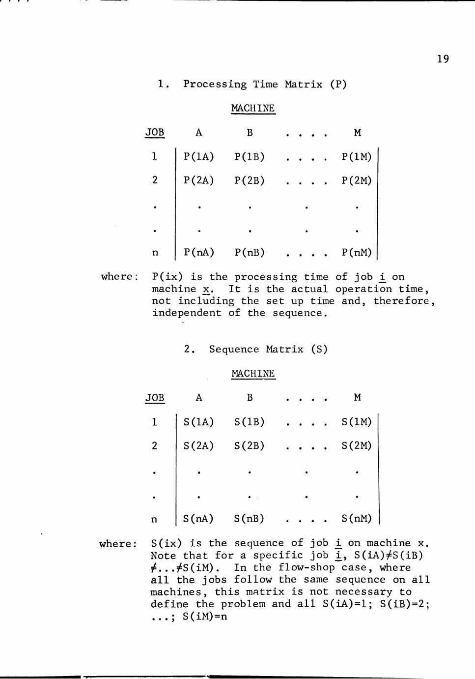
1. Processing Time Matrix (P)
MACHINE
JOB B • • . M
n
P(1A) P(1B)
P(2A) P(2B) • • • •
P(nA) P(nB)
P(1M)
P(2M)
P(nM)
where: P(ix) is the processing time of job on machine x. It is the actual operation time, not including the set up time and, therefore, independent of the sequence.
2. Sequence Matrix (S)
MACHINE
JOB B . . . M
n
S(1A) S(1B)
S(2A) S(2B)
S(nA) S(nB)
• •. •
S(1M)
S(2M)
S(nM)
where: S(ix) is the sequence of job on machine x. Note that for a specific job ±, S(iA)f S(iB) 7 . . .9 S(iM) . In the flow-shop case, where all the jobs follow the same sequence on all machines, this matrix is not necessary to define the problem and all S(iA)=l; S(iB)=2; ...; S(iM)=n

20
3. Set up time or set up cost matrices for each machine
involved in the process (Tx or Cx)
As an example, for the set up time case, the problem
would be defined by m (number of machines) matrices of the
following format, one for each machine:
MACHINE X
Preceding Job
0
1
2
Following Job
n
T(Ox,lx) T(0x,2x) T(0x,3x)
T(2x,lx)
T(lx,2x) T(lx,3x)
T(2x,3x)
n
T(Ox,nx)
T(lx,nx)
T(2x,nx)
T(nx,lx) T(nx,2x) T(nx,3x)
where: T(ix,jx) is the set up time for job j_ on machine x if its predecessor on this machine was job i
Note that T(Ox,jx) indicates that job j_ is not preceded
by any other on a specific machine x^, i.e., job j_ is the
first job to go on this machine. Also, T(ix,ix) does not
exist, since predecessor and following jobs cannot be the
same.
Besides these matrices, if there is dependence among the

21
operations, these requirements are also stated. The list of
dependence would contain as many expressions of the following
type as necessary:
"ix precedes 2I." (job i on machine x precedes job j_
on machine ^ ) .
As an example, if job 3 on machine A precedes job 2 on
machine C the expression showing the dependency would be:
"3A precedes 2C".
If i and j_ refer to the same job, the expression is not
necessary, since this situation is covered by the Sequence
Matrix (S). In addition to the basic data matrices and any
dependency requirements, the statement of the problem also
includes a list of assumptions which characterize the specific
problem (a list of the usual assumptions made in sequencing
was stated earlier in Chapter I).
Set up Times
This analysis will now concentrate on the situations in
which the operation set up is due mainly to time. The costs
involved in the set up are, therefore, primarily obtained
from labor and man-hours and the problem can be easily
formulated through set up times, if needed.
22
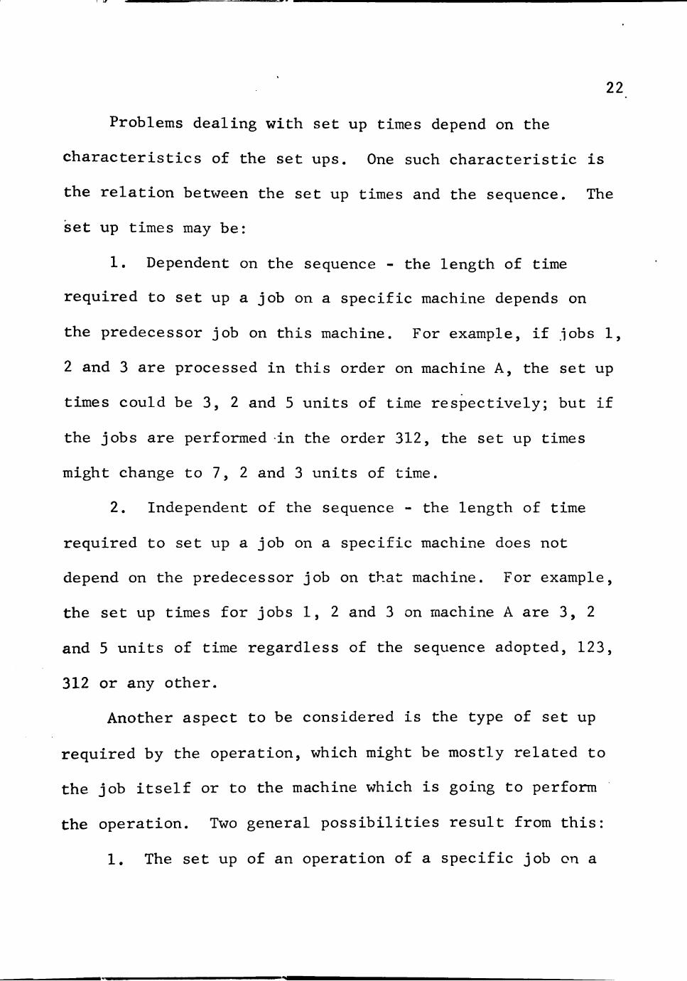
Problems dealing with set up times depend on the
characteristics of the set ups. One such characteristic is
the relation between the set up times and the sequence. The
iset up times may be:
1. Dependent on the sequence - the length of time
required to set up a job on a specific machine depends on
the predecessor job on this machine. For example, if jobs 1,
2 and 3 are processed in this order on machine A, the set up
times could be 3, 2 and 5 units of time respectively; but if
the jobs are performed in the order 312, the set up times
might change to 7, 2 and 3 units of time.
2. Independent of the sequence - the length of time
required to set up a job on a specific machine does not
depend on the predecessor job on that machine. For example,
the set up times for jobs 1, 2 and 3 on machine A are 3, 2
and 5 units of time regardless of the sequence adopted, 123,
312 or any other.
Another aspect to be considered is the type of set up
required by the operation, which might be mostly related to
the job itself or to the machine which is going to perform
the operation. Two general possibilities result from this:
1. The set up of an operation of a specific job cn a

irTirti.ii I i i f ' ^ a :
23
specific machine may start only after the predecessor
operation of this job on another machine has finished; the
job is required for the set up. An example of this situa
tion is as follows. A single metal plate, after previous
operations has to be placed on a machine to be drilled
according to some specifications. Since the job consists
of only one plate, no fixtures are used. The set up of this
drilling operation cannot start without the metal plate
itself.
2. The set up of an operation of a specific job on a
specific machine may start (and finish, if the time permits)
before the predecessor operation of this job on another
machine has finished. The set up relates mainly to the
machine, and the time required for the set up with the job
present is negligible. An example follows: suppose that
several plates had to be manufactured in the example for the
previous case. A fixture could be adapted to the machine
taking care of the specifications. The set up for the
drilling operation is performed now without the plates.
When one is dealing with set up times, there is still
the question of the objectives to be achieved. One such
objective is the minimization of the total elapsed time.

I I I I I I
24
Set up Times and the Minimization of Total Elapsed Time
From the considerations made on set up times, four
general cases can occur:
Case 11: The set up time is sequence dependent and can
start only when the job has finished its processing on the
previous machine.
A 3-job, 3-machine flow-shop problem defined by the
following matrices is used to illustrate the situation.
Processing Time Matrix (P)
JOB
1
2
3
MACHINE
A
19
27
8
B
25
12
45
C
33
26
21
MACHINE A
Set up time Matrices (Tx)
MACHINE B
Following Job Following Job Preceding Job 1 2 3 Preceding Job 1 2 3
0 3 7 5
9 7
0 7 1 9
6 10
10
2 6 5 6

MACHINE C
-Mm^i^^^Mi^LJ
25
Following Job
Preceding Job
0
1
2
3
4
7
10
7
10
The problem was solved by enumerating, the possible
sequences with no passing allowed and the best solution was
found to be sequence 123 with a total elapsed time (including
the set up times) of 159 units of time. Figure 1 presents a
Gantt chart for this solution. It can be noticed from
Figure 1 that the set ups of all jobs on machines B and C
started only after these jobs were finished on machines A
and B respectively.
Case 12: the set up time is sequence dependent, but the
set up can be carried out on the next machine if this machine-
is free, although the job is still running on the previous
machine.
The problem used as an illustration for case 11 was
solved under the new conditions. It was determined that for

26
Machines
B
Note:
'A
ii 3 19
i 27
22
25
9 8
set up times
6 12
33
45
26
58 54
75 76
10 21
Time
93 128 128 159
Figure 1. Gantt Chart for Case 11 - Best Sequence 123
this case the best sequence was no longer 123, but sequence
321, which resulted in a total elapsed time of 144 units.
However, a Gantt chart for sequence 123 is presented in
Figure 2 so that the characteristics of cases 11 and 12
might be better compared. It may be noted that for the same
sequence, the total elapsed time for case 12 is smaller than
the total elapsed time for case 11.
Case 21: the set up is independent of the sequence and
can start only when the job has finished its processing on

» F P F
27
Machines
i
B
3 19 9
1 W/. 11 9 8
M 25
22
i 7
12 5+2 45
^ili
33 26 10 7+3 21
58 75 47 70
Time 122
80 115 146
Note:
tZ.M \
L...J
set up performed when both machine and job are available
set up performed during machine idle time
indicates that the set up could have started earlier
Figure ?.. Gantt Chart for Case 12 - Sequence 123
the previous machine.
This case reduces to the sequencing problem in which
production times can be used. Since the set up times do not
depend on the sequence adopted, one matrix is sufficient to
define these times. Each job has now a single defined set
up time on each machine. As an example, the same problem
of cases 11 and 12 could be used as far as the processing

F F F F r
28
times are concerned. For the set up times, the following
matrix replaces the three separate matrices on set up
times:
Set up Time Matrix (T)
JOB
1
2
3
MACHINE
A
1
8
10
B
6
12
6
C
5
15
13
The best sequence for this problem is 123 and it is
shown in the Gantt chart of Figure 3. The chart is presented
in a different fashion compared to the previous charts,
since now the block representing the job and its set up is
divided into three parts. The lower part shows the character
istic of this case which is that the set up time and the
operation time may be considered together as a general pro
duction time for each job on each machine. In fact, this
problem can be solved by any known sequencing algorithm for
flow-shop cases (for the specific example) with the data
being presented in a single matrix, resulting from the
summation of each operation time with its set up time, as

Machines
B
1 19 8 27 10 8
Note: ^ ^
w iM 20 35
^ 21
31
jm
zrr
18
* Lil 12
24
33
Al
51
15 26
38
55 73 79
41
29
13 21
^
M.
Time-
89 l50 130 164
set up time
Figure 3. Gantt Chart for Case 21 - Best Sequence 123
follows:
Production Time Matrix (processing times plus set up times)
MACHINE
JOB
1
2
3
A
19+1=20
27+8=35
18
B
31
24
51
C
38
41
21+13=34

30
Case 22: the set up time is independent of the sequence,
but the set up can be carried out as soon as the machine is
free, even though the job is still.running on the previous
machine.
In this case, production times cannot be used although
the set up times do not depend on the sequence adopted. The
reason is that these set ups may now occur during the machine
idle periods, whenever this is possible, as it was observed
in case 12. In situations like this, probably quite con
ceivable in industry, the total production time should be
separated into set up time and the actual processing time
of the operation. These considerations give a more realistic
view of the times when the machines are not executing any
job. These times are not necessarily idle, as considered in
the conventional sequencing problem, since set up operatiors
might be taking place.
Figure 4 shows the Gantt chart for the above case with
the same sequence adopted in case 21, with a total elapsed
time of 153 units of time. The best solution for case 22 is,
however, sequence 213 with a total elapsed time of 152; only
the Gantt chart for sequence 123 is presented, since it
serves best as comparison between cases 21 and 22.

31
Machines
B
19 .g, 21 ^
12 6 10+2 12 4+2 45
Note
t///r......j
[:
set up performed when both machine and job are available
set up performed during machine idle time
indicates that the set up could have started earlier
Figure 4. Gantt Chart for Case 22 - Sequence 123
Minimization of Total Set up Time
Another objective or criterion one might want to achieve
when dealing with set up times is the minimization of the
total set up time involved in the sequence. This objective,
from a sequencing standpoint, would only be pertinent in the

32
case in which the set up times are sequence dependent. If
the set up times are independent of the sequence, since they
are considered to be known and fixed, the total set up time
is the same for any sequence chosen. Therefore, the
comments that follow relate only to the sequence dependent
cases:
1. Flow-shop: to minimize the total set up time, one
approach might be to combine the matrices defining the set
up times into one single matrix by adding their elements,
since all jobs must have the same sequence on the machines.
The problem would then consist of finding the best sequence
based on this matrix. If the elements of the three set
up time matrices presented as an example for case 11 are
added, this results in the following:
Single set up time matrix (for machines A, B and C)
Following Job
Preceding Job
0
1
2
3+7+6=16
2+10+4=16
14
11
24
13
24
24
26
-/-.-^-r..:. "-J-f-
33
The minimum total set up time is 51 for both sequences
213 and 231. Of course these sequences are not the same as
when the total elapsed time was considered as the optimizing
criterion. In fact, the best sequence for case 11, 123, is
the one with the highest total set up time, 66 units.
Therefore, usually one cannot achieve both objectives with
the same sequence. If it is desirable that the total set up
time and the total elapsed time are both kept to a composite
minimum, a new sequence will probably have to be chosen.
Such a sequence would be 321 considering case 11 and the
total set up time, with total processing time of 162 and
total set up time of 53.
If the first row of the single set up time matrix
presented above is disregarded, a situation similar to the
traveling salesman problem occurs. The word "similar" was
used since the traveling salesman problem implies a contin
uous repetition of the sequence adopted (jobs 1, 2 and 3
would be executed several times according to a certain
sequence, as for instance 1231...), while in sequencing
there is no such cycle.
2. Flow-shop with passing allowed and job-shop: each
matrix would have to be considered separately and the best
niTi
34
sequence for each machine should be selected. However, the
problem of feasibility has to be taken into consideration,
since the sequences obtained through the set up times are
not always feasible.
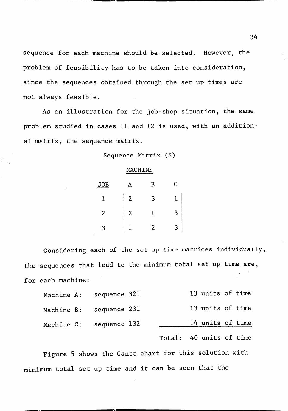
As an illustration for the job-shop situation, the same
problem studied in cases 11 and 12 is used, with an addition
al matrix, the sequence matrix.
Sequence Matrix (S)
JOB
1
2
3
MACHINE
A
2
2
1
B
3
1
2
C
1
3
3
Considering each of the set up time matrices individually,
the sequences that lead to the minimum total set up time are.
for each machine:
Machine A: sequence 321
Machine B: sequence 231
Machine C: sequence 132
13 units of time
13 units of time
14 units of time
Total: 40 units of time
Figure 5 shows the Gantt chart for this solution with
minimum total set up time and it can be seen that the

-^ 9
35
Machines
B
5 8 6 27 19 ^
1 12 7
I 45
Set up time
5+6+2=13
5 2+3 25
1
33
13 13
46
21
67 65
1+7+5=13
26
Time 95
6+7+1=14 Total: 40
39 86 113
Note t j ^ - ^ ' . ^ ;
1 [:::]
set up performed when both machine and job are available
set up performed during machine idle time
indicates that the set up could have started earlier
Figure 5. Gantt Chart - Job-shop Case - Minimum Total Set up Time
sequence is feasible.
Consider now for the same basic data a different
sequence matrix defined as follows:

1 ff
Modified sequence matrix
36
MACHINE
JOB
1
2
3
A
2
1
2
B
3
2
1
C
1
3
3
The sequences which lead to the minimum total set up
time are, of course, the same, but as it can easily be seen,
the solution now is not feasible. The fact is, as indicated
by the sequence matrix, that job 2 has to go first on
machine A, then on machine B. The sequence that leads to
the minimum total set up time on machine B is 231, therefore,
job 2 is the first job to be performed on this machine.
Since job 3 has to go first on machine B and also follow job
2 on this machine, it is not possible for job 3 to precede
job 2 on machine A; consequently, the solution is not feasible.
Figure 6 shows schematically this infeasibility.
The solution to the problem would be then the one among
the feasible solutions which has the minimum set up cost.
For the example, since the infeasibility occurs between jobs
2 and 3 on machines A and B, it is sufficient that one of
the sequences (32 on machine A or 23 on machine B) be reversed

37
Machine
>
1 1
B
f
Not
Job 2
feasible
Job 2 Job 3
1
Job 3
Sequence
321
231
Job 2: ABC Job 3: BAG
Figure 6. Schematic Representation of Infeasible Solution
The next best solution is found by putting job 2 before job
3 on machine A with the sequence 213 and a total set up
time of 3 units of time more than the infeasible solution
presented earlier. Figure 7 presents the Gantt chart for
the feasible solution.
Minimization of total set up time should be considered
as the main objective to be achieved when the time involved
in the set up is very costly. Oi.e such situation occurs
when the set up times are extremely long in relation to the
processing times and a significant difference is observed in
the set up times from one sequence to the other. In other
situations, the set up times are not too long but a large
group of workmen might be needed for the set ups. When this
occurs consistently for all jobs in the shop, the labor costs
involved in the set ups are still proportional to times.
The minimization of total set up time is also a sound criterion

38
Machines
B
27 2 19 %
••:M
33
12 7
\. 2 "WW/
34
39
58 46
Note:
45
7 8
m.
Set up time
7+2+7=16
25
1+7+5=13
21 1 26
106 98 128
127
Time
154
6+7+1=14 Total: 43
'^•'/:/:'\ ^^^ P performed when both machine and job are ^'''"''"' available %y/,</r.
set up performed during machine idle time
[_ _J indicates that the set up could have started earlier
Figure 7. Gantt Chart - Job-shop Case - Best Feasible Solution for Modified Sequence Matrix
for these cases. Finally, one should minimize total set up
time if this brings more reduction in the total cost of
production than any other criterion of sequence evaluation.
Objectives other than minimizing total elapsed time or
total set up time may also be considered when one is dealing
with set up times. Such criteria as meeting of due dates or

v-n/nrr^;.'.. y^»
39
minimizing total inventory cost are conceivable. However,
they are beyond the scope of this work and will not be
examined here.
Set up Costs
The situation in which the schedule is selected based on
set up costs will be considered now. Set up costs are mainly
used when the material for the set up of an operation is
much more expensive in comparison to the time involved. The
analysis depends again on the criterion used for sequence
evaluation. If one is trying to minimize the total elapsed
time, the set up costs will be disregarded, since through
the definition of the problem they are not time-related.
Therefore, the criterion that requires some further comments
is the minimization of total set up costs. The problem is
somewhat similar to the minimization of total set up time
and, again, is only pertinent to sequencing if the set up
costs are sequence dependent. The same comments and
restrictions on flow-shop and job-shop situations made in
the discussion of the minimization of total set up time apply
to the minimization of total set up costs. The only difference
is that the set up matrices are in terms of costs and not
times. However, it seems that some further consideration
should be given to machine idle costs, for the set up cost

'~l /»
40
minimization may lead to a sequence where idle time is very
high. Figure 7 gives an indication of this possibility. If
these idle costs are sufficiently large to affect the overall
cost of production, another sequence should be selected such
that a lower total cost is obtained.
The criterion of minimizing total set up costs would be
a sound one in cases in which these costs differ noticeably
depending on the sequence adopted and a large amount of money
is involved. Some situations in which labor is the main
factor in the set up may be analyzed through set up costs.
In these situations, the labor involved in the set ups varies
from operation to operation. Some jobs require heavy set ups
that take many workers to perform. Others, however, can be
done by one or two men, even though they might take a con
siderable amount of time. In these cases, therefore, time
is not a good criterion for the evaluation of the sequence.
The minimization of total set up cost is what should be
achieved.
Dynamic Situations
Most sequencing research considers the shop as a "closed
system" with respect to jobs, i.e., the jobs are all avail
able at the same time and no consideration is given to future

^1
jobs that might come to the shop. This static way of looking
into sequencing problems has applications in some industrial
situations; it is found in specific shops or as a subset of
a larger decision process (a day by day scheduling procedure,
part of an overall weekly or monthly scheduling plan). It
seems relevant, however, to give some attention to dynamic
situations in this analysis.
One possible procedure to follow in a dynamic situation
is that each time a new group of jobs enters the shop, a
reevaluation of the present schedule should be made. Infor
mation on the operations already terminated should be
obtained, since they would be disregarded for the new
sequence. It should be noticed that this kind of reevalua
tion is quite expensive, for it generally assumes a computer
ized system. However, some large companies have this type
of feedback that enables them to know the location of a job
at a specific stage of production. Smaller companies could
always obtain this information manually or through periodical
reports.
For the new schedule, the jobs which are presently
engaged on machines would have to be reconsidered. If these
jobs cannot be removed from these machines before their com
pletion, they should be scheduled first, either through

42
priority rules or the times they still require on these
machines could be blocked. If the jobs can be removed from
the machines before their completion, the remainder part of
these jobs would be considered as their processing times
along with the set up requirements. Of course, the set up
times for these jobs, if they are to start on the same
machines they were on, are zero. This, depending on other
times involved, puts them in a privileged position to remain
at those machines in the new schedule.
In practical situations, problems like machine break
down, operator absenteeism, non-deterministic processing
times, the existence of more than one machine of each type
and many others are also likely to occur. Whether one needs
to include all these restrictions in a theoretical model or
not, the cV7areness of their existence is of vital importance.
CHAPTER III
AN INDUSTRY SURVEY ON SET UP TIMES AND SET UP COSTS
There i s ^ growing tendency at present for research to
direct its efforts toward problems of a practical nature.
This trend is observed not only in industrial circles but
also in governmental areas. Acknowledging the importance of
communication between industry and university, a questionnaire
was prepared covering the specific area of sequencing with
which this research is concerned. The purpose of the survey
was to find out the importance that industry gives to the
problem of set up tim.es and costs and to bring new guide
lines for future research.
The questionnaire was developed, reviewed and modified
before the final format was chosen. Personal interviews
with representatives of two local companies were held in
order to test the questions and material covered by the
questionnaire. Terminology differences as well as a con
ceptualization of the problem are usual barriers when such
a contact is established. Further modifications resulted
from these interviews. The word "sequencing" was generally
avoided and substituted by "scheduling", more readily
43

44
recognized by people in industry.
The Objectives
The questionnaire was prepared in order to obtain an
overall look at the importance of set up costs and set up
times to industrial situations. The intent was to cast some
light on relevant points related to set up procedures in
sequencing evaluations. One of these points was the ranking
of importance that industry gives to this criterion compared
to others such as the minimization of total elapsed time or
meeting of due dates. ^
A question not related specifically to the problem of
set ups, but to sequencing in general, that of the average
size of the shop was also included. The number of jobs and
machines involved in a sequencing decision is of vital
importance, since it represents the major restriction for
practical uses of most algorithms developed so far. As soon
as more than a certain number of jobs and machines (10 of
each on the average) are involved, some procedures can no
longer be used. The computational time necessary for their
solutions in existing computers becomes economically
prohibitive.
Another point of interest included in the questionnaire
45
relates to the differentiation between set up times and set
up costs. The companies were asked to give the percentage
of the situations in which set up costs are a function of
time (and labor) and therefore can be treated as set up
times against the situations where they are a function of
material with no significant relation to time.
A question on set up seqitence dependence was also
included in the questionnaire. The purpose of this question
was to find out whether there is complete independence,
complete dependence or a combination of both. Some jobs
might require similar set ups and the order in which these
specific jobs are scheduled would not really matter as far
as the set up times are concerned.
The objectives of the survey were, therefore, to learn
some practicc.l aspects about the problem, when set up con
siderations should be made, how many variables are involved
and how they are related. The answers to these questions
should bring a better insight to the matter under study.
Analysis of the Results
The questionnaire in its final format was sent to
industries of various sizes and types in the country. The
list of the participating industries is not presented since

46
the information and their sources was promised to be kept
confidential. Before the results are presented, some comments
should be made about the selection.of these industries. In
1969, a questionnaire was prepared by the Sequencing Research
Group of the Department of Industrial Engineering of Texas
Tech University. A little over 300 copies were sent at that
time to well known companies that could be concerned with
sequencing procedures. The survey related mainly to the
usual assumptions of the flow-shop and job-shop problems.
The companies selected for the present questionnaire were
mainly chosen among those that answered the first survey,
i.e., companies that showed an interest and concern about
sequencing. Seventy-six questionnaires were sent this time
based on this criterion. Another 32 questionnaires were
sent to personal acquaintances of faculty members of the
Department, leading to a total of 108 copies sent. Forty
answers were received, about 377o of the questionnaires sent.
The results of the questionnaire are now presented
question by question. An analysis of the answers follows
each question.
1. When a number of jobs are being scheduled for several
operations in a specific shop, how many jobs and machines are

47
generally involved, at a given time?
Jobs Machines No. of answers
1-10 1-10 7
11-20 1-10 1 21-30 2 31-40 1
21-40 1-10 1 11-20 2 31-40 1
41-80 31-40 2 more than 40 3
more than 80 1-10 5 21-30 1 31-40 1 more than 40 10
In relation to the size of the problem, one can see a
trend to the large sized problem as being the most common
one. Question 1 was not concerned with the company as a
whole but was limited to a specific shop and to situations
in which a number of jobs were being scheduled on a number
of machines at a given time, even though, 257o of the answers
were in the class of more than 80 jobs and more than 40
machines. Fifty-five per cent of the companies showed that
they have 40 jobs or more being scheduled at the same time,
and 537o acknowledged 20 machines or more in their shops.
However, situations with 10 jobs and 10 machines at the most

48
do exist. Eighteen per cent of the answers were in the
(l-lO)x(l-lO) bracket which is interesting and somewhat
promising for the application of some existing sequencing
algorithms. A special analysis of these cases will be made
after the results of all questions have been presented.
2. In this shop, are most of the machines of a differ
ent type?
Yes 24 answers
No 16 answers
Question 2 concentrated on the similarity of the
machines in the shop. Sixty per cent of the companies stated
that most of the machines in their specific shops were
different. This is an important result, for most sequencing
research is based on the assumption that there is only one
machine of each type. Of course, this information should be
accepted with a certain care. Since most of the companies
reflected reasonable large sized shops, it is quite probable
that many of their machines are identical or at least similar.
In this same line of thought, some of the "Yes" answers to
this question had to be counted as negative. A classification
by type of machine was included and this did not represent
the situation in which one machine of each type is assumed.

49
These apparently ambiguous answers are, however, quite under
standable. Consider, for example, a shop with 80 machines
where there are 70 different types.of machines. Some of the
machines in this shop are evidently alike. However, it is
quite conceivable for industrial purposes that these 80
machines would be considered as being mostly of different
types.
3. Rank in importance (l-highest/4-lowest) the
following criteria for a scheduling decision:
A. Minimization of total processing time
B. Meeting of due dates and/or minimization of penalty costs
C. Minimization of total set up tir.o and/or total set up costs
D. Minimization of in-process inventory costs
No. of answers for each rankin'
Criteria Rankings: 1
A. Minimization of total processing time
B. Meeting of due dates and/or minimization of penalty costs
C. Minimization of total set up time and/or total set up costs
D. Minimization of in-process inventory costs
6 14
33
9 11
1
4 12 15
4
8 11 19
50
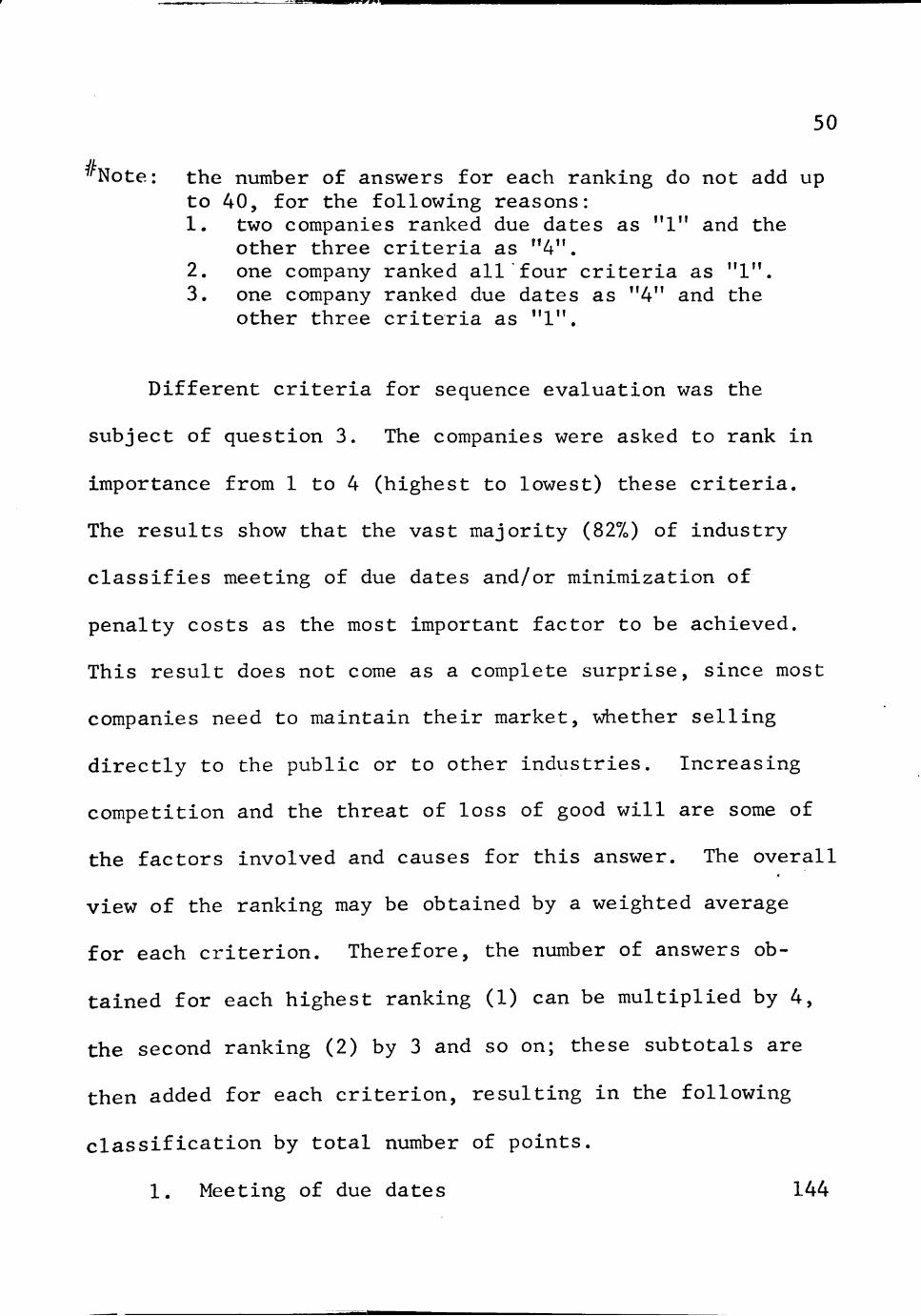
^^Note: the number of answers for each ranking do not add up to 40, for the following reasons: 1. two companies ranked due dates as "1" and the
other three criteria as "4". 2. one company ranked all four criteria as "1". 3. one company ranked due dates as "4" and the
other three criteria as "1".
Different criteria for sequence evaluation was the
subject of question 3. The companies were asked to rank in
importance from 1 to 4 (highest to lowest) these criteria.
The results show that the vast majority (827o) of industry
classifies meeting of due dates and/or minimization of
penalty costs as the most important factor to be achieved.
This result does not come as a complete surprise, since most
companies need to maintain their market, whether selling
directly to the public or to other industries. Increasing
competition and the threat of loss of good will are some of
the factors involved and causes for this answer. The overall
view of the ranking may be obtained by a weighted average
for each criterion. Therefore, the number of answers ob
tained for each highest ranking (1) can be multiplied by 4,
the second ranking (2) by 3 and so on; these subtotals are
then added for each criterion, resulting in the following
classification by total number of points.
1. Meeting of due dates 144
51
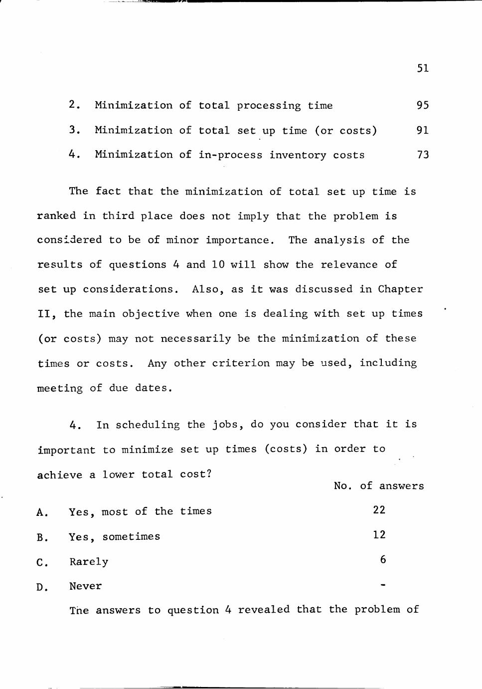
2. Minimization of total processing time 95
3. Minimization of total set up time (or costs) 91
4. Minimization of in-process inventory costs 73
The fact that the minimization of total set up time is
ranked in third place does not imply that the problem is
considered to be of minor importance. The analysis of the
results of questions 4 and 10 will show the relevance of
set up considerations. Also, as it was discussed in Chapter
II, the main objective when one is dealing with set up times
(or costs) may not necessarily be the minimization of these
times or costs. Any other criterion may be used, including
meeting of due dates.
4. In scheduling the jobs, do you consider that it is
important to minimize set up times (costs) in order to
achieve a lower total cost? No. of answers
A. Yes, most of the times 22
B. Yes, sometimes 12
C. Rarely 6
D. Never
The answers to question 4 revealed that the problem of
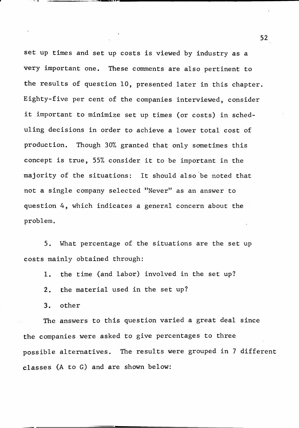
52
set up times and set up costs is viewed by industry as a
very important one. These comments are also pertinent to
the results of question 10, presented later in this chapter.
Eighty-five per cent of the companies interviewed, consider
it important to minimize set up times (or costs) in sched
uling decisions in order to achieve a lower total cost of
production. Though 307, granted that only sometimes this
concept is true, 557o consider it to be important in the
majority of the situations: It should also be noted that
not a single company selected "Never" as an answer to
question 4, which indicates a general concern about the
problem.
5. What percentage of the situations are the set up
costs mainly obtained through:
1. the time (and labor) involved in the set up?
2. the material used in the set up?
3. other
The answers to this question varied a great deal since
the companies were asked to give percentages to three
possible alternatives. The results were grouped in 7 different
classes (A to G) and are shown below:

•V«BB
53
1 .
2 .
3 .
No.
TIME
MATERIAL
OTHER
of a n s w e r s
A
1007o
-
-
' '
B
75-957,
5-257o
5-107o
16
C
507o
507.
-
1
D
257o
257o
507o
1
E
-
207o
807o
1
F
-
-
1007o
2
G
did
not
answer
2
The costs related to set up procedures are mainly a
result of the time involved. Eighty-two per cent of the
answers to question 5 indicated that the situations in which
set up costs are obtained through the time (and labor) used
in the set up are the most common ones. Seventy-five per
cent or more of the set up cost was due to time in these
situations. It is important also to mention that 437o of the
companies attribute these costs entirely to set up times (or
as the question was put, the other costs are negligible).
These results show that research efforts to solve the set up
problem should be mainly directed to situations in which the
set ups are expressed through times. The choice of the third
alternative, "Other", was explained in terms of considering
average set up costs per machine centers or through major
equipment burden rates, which may include time. The set up
costs in these cases are spread over the entire production
s an overall cost.
54
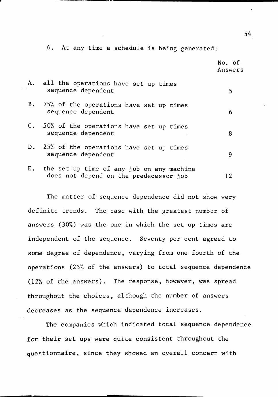
6. At any time a schedule is being generated:
No. of Answers
A. all the operations have set up times sequence dependent 5
B. 757o of the operations have set up times sequence dependent 6
C. 507o of the operations have set up times sequence dependent 8
D. 257o of the operations have set up times sequence dependent 9
E. the set up time of any job on any machine does not depend on the predecessor job 12
The matter of sequence dependence did not show very
definite trends. The case with the greatest number of
answers (307o) was the one in which the set up times are
independent of the sequence. Seventy per cent agreed to
some degree of dependence, varying from one fourth of the
operations (237o of the answers) to total sequence dependence
(127o of the answers). The response, however, was spread
throughout the choices, although the number of answers
decreases as the sequence dependence increases.
The companies which indicated total sequence dependence
for their set ups were quite consistent throughout the
questionnaire, since they showed an overall concern with

55
the problem. On the other hand, all companies granted some
importance to set up considerations in scheduling evalua
tions, as one can see from the results of question 4. This
concern, together with the fact that 307o of the companies
acknowledged set up times which are independent of the
sequence show that the problems of case 22 (of the analysis
on cet up times made in Chapter II, page 30) should deserve
quite a bit of attention.
7. In your shop, when each job is to be processed on
all (or most of all) of a group of machines, what is the
trend observed for each machine?
No. of answers
A. all jobs require similar set ups 5
B. 757o of the jobs require similar set ups 9
C. 507o of the jobs require similar set ups 7
D. 257o of the jobs require similar set ups 15
E. all jobs require completely different set ups 4
Only 107o of the answers to question 7 showed that all
jobs require a completely different set up. The remaining
907, indicated the existence of at least some jobs with
similar set ups. Set up similarity was the term used in
the questionnaire to characterize the possibility of the
56
set up of a job on a specific machine to be wholly or
partially used for the next job on this machine. The
situation in which only 257o of the operations have similar
set ups was the one with the largest number of answers
(387o), although 237, showed that 757o of their jobs have
this characteristic, with 177, in the middle position and
127, listing complete similarity.
Questions 6 and 7 are somewhat correlated and a com
parison was made in order to clarify some ideas in relation
to similarity and sequence dependence. In fact, it was
verified that the four companies which showed that all
their jobs require completely different set ups, also
indicated that their set up times (or costs) did not depend
on the sequence. Also, most of the remaining companies
which had selected set up sequence independence on questic.
6, reported to have only 257o of the jobs with similar set
ups. The case in which all operations have set up times
sequence dependent was not fully connected with complete
similarity; it varied from that extreme case to half of the
jobs requiring similar set ups. This result is quite
reasonable, for total sequence dependence does not require
complete similarity. A small example is presented. Two

57
jobs, 1 and 2, have similar set ups on a certain machine x,
which means that their set ups can be wholly or partly used
one for the other when they are scheduled in sequence. How
ever, it is possible that due to the characteristics of the
jobs (and the machine), if job 1 is to follow job 2, only
a small part of the set up of job 2 can be utilized for
the set up of job 1. If, on the other hand, job 2 follows
job 1, it might happen that a great part of the set up is
utilized, resulting, therefore, in sequence dependent set
ups, even though they are similar. The joint analysis of
questions 6 and 7 showed, however, that in general there
is some relation between the factors. This is indicated by
the fact that 807, of the answers presented results that
were in the same bracket of percentages for both questions
(for example, sequence dependence: 257,; similarity: 257o)
or deviated by only 257o (for example, sequence dependence:
507,; similarity: 257o).
8. If in a number of jobs, some require similar set ups,
do you schedule these one after the other?
Yes 31 answers
No 9 answers

58
The response to question 8 indicated that jobs that
require similar set ups are generally scheduled one after
the other. This procedure was supported by 787, of the
answers. There are, however, some constraints to this
practice and these are analyzed in the following question.
9. If the answer to question 8 was "No", please state
your reasons.
Meeting of due dates seems to be the main cause for
not scheduling similar jobs together and most replied that
whenever these constraints are not present, similarity
would be the main factor to be considered. The possibility
of overriding these due dates to save an expensive partial
set up was also mentioned.
10. Is there any situation ivi your shop where the
costs involving machine set up are the most important
factor in a scheduling decision?
Yes 20 answers
No 20 answers
Fifty percent of the companies agreed that they have
situations in which set up considerations are the most im
portant factor in sequence evaluation. Some examples were
59
given and they refer mainly to oversized machines that re
quire a very heavy and elaborate adaptation for different
jobs. Another example refers to jobs, with extremely long
set ups, which are generally delayed to maximize shop
throughput. Sometimes, only a small amount of a product
is needed for an order; if a large quantity were produced,
it would eventually become obsolete. The set up costs in
these situations can be quite high when compared to the
cost of production.
Small Shops
Some comments are now made on the answers which showed
a problem size with at most 10 jobs and 10 machines. This
analysis is made taking into consideration that these are
the cases which can be handled by most of the current
optimizii'g sequencing procedures. The assumption of one
machine of each type was found to be true for most of the
small shops. The ranking of the different criteria for
scheduling evaluation was concentrated on due dates. The
analysis of these specific cases did not show, in general,
too much deviation from the overall results of the question
naire. For practical applications to the small problem,
the criterion of minimizing due dates is worthy of research.
The case in which 507o of the operations have set up times

60
sequence dependent, was the most common situation. The
trend to schedule jobs that require similar set ups in
sequence was even stronger for the small shop, since all
the answers of this group to question 8 were affirmative.
Set up Times and Costs in Scheduling Decisions
The last part of the questionnaire, question 11, was
aimed at obtaining information on practical industrial
situations in which set up times (or costs) represented an
important part of the scheduling decision. The response was
quite good and some of the examples are now presented.
In a typical department of a brewery, the main oper
ations are canning and packaging, in which cans are filled
with beer, closed, pasteurized, packaged and palletized
in a convertible can line capable of producing 12 oz.,
14 oz. and 16 oz. cans. Conversion from one can size to
another requires up to one shift with several maintenance
employees. Furthermore, hourly employees idled by a
conversion are paid for a full shift, as specified by Union
contracts. Thus, when scheduling for multiple package
production on this line, one must consider the conversion
(set up) costs of maintenance manpower and idled labor;
also to be considered is the reduction of available production

61
time due to a changeover, which may be critical during
periods of heavy demand.
In scheduling a paper machine to manufacture several
different colors of paper in several different basic
weights, the sequence is very important to minimizing costs.
The change time from one color to another is more signi
ficant than from one weight to another. Therefore, if
colors A, B, C are each to be made in weights 1, 2, 3, the
sequence should be Al, A2, A3, Bl, ..., C3 rather than
Al, Bl, CI, A2, B2, ..., C3. This example is somewhat
similar to the manufacture of paint presented in Chapter I.
In steel manufacturing, rolling mill facilities are
used where guides for particular sizes must be changed.
The set up consists mainly of changes in sets and sizes.
A set of guides includes a number of sizes and may take
eight hours or more to complete. However, setting up for
a size within that set can take between a half hour and an
hour. When determining an economical rolling quantity for
a set change, time and cost are the primary determinants.
This is also true of quantities for sizes within the set.
For example, 50,000 pounds might be required per eight
hour shift and 10,000 pounds per size to justify a set up
and subsequent size changes.
-
62
An example which encompasses set up times and due dates
was presented by a tire manufacturer and was based on the
operations which extrude treads for tires. The rubber stock
progresses through two mills before being extruded through
a die. Each die is serviced by two mill lines so that two
types of rubber can be combined to produce a single tread.
The manufacturer adds that if the set up time is not mini
mized, there would not be enough production time left
during the shift to meet the schedules.
A glass container manufacturer presents an example
related to the shop where boxes are made for the containers
they produce. Their corrugator takes roll stock bulk paper
of various grades, depending on the type of corrugated board
desired for the boxes, and after several stages, it pro
duces corrugated boards. Set up times can vary in length
quite a bit and unless jobs are scheduled properly, the
operation could become very costly. Jobs are scheduled
first according to the type of paper and then to job change
time. Since this machine runs at a very high rate of speed,
the faster job changes (set up) are completed, the less
downtime and the quicker the maximum speed can be regained.
Therefore, similar jobs are preferably scheduled in sequence
In winding circular coils for core form construction

63
transformers, set up times (costs) represent a significant
percentage of the total time required to wind each coil.
The primary reasons are: (a) to wind each coil requires
set up on the winding machine plus set up on special fix
tures used to support and feed the conductor material to
the winding machine; (b) even though circular coils are
different for various jobs and require different conductor
material, the number of fixtures used to support and feed
the reels of conductor material could be the same from job
to job. By utilizing existing set up, costs can be reduced
if similar jobs are produced in the proper sequence within
a limited time span.
Production areas such as die casting operations, which
involve fairly long set ups relative to operation times
increase tbe degree of set up cost considerations. Pro
duction operations dependent on furnace temperatures or
chamber pressures are also highly dependent on set up con
siderations.
Concluding Remarks
The results of the survey revealed some very interest
ing information. They show quite consistently that the pro
blem of set up times and set up costs is viewed with concern

64
by industry in general. Some more questions were raised
during the development of the research, after the question
naires had been sent. For example, do the companies
actually have the data required for the set up time matrices?
Do the set ups relate mostly to the jobs or to the machines?
The answers to these questions could provide further under
standing of the problem under consideration.
One important point resulting from the survey is that
the costs involved in the set ups are primarily related
to times. The following chapter presents some possible
techniques to solve specific kinds of problems dealing with
set up times.

^.•»^\ Biaaairigti ^ X ^ l
CHAPTER IV
POSSIBLE SOLUTIONS TO THE PROBLEM WITH SET UP TIMES SEQUENCE DEPENDENT
This chapter will be concerned with procedures to solve
sequencing problems with set up times dependent on the
sequence, where the evaluation criterion is the minimization
of the total elapsed time (Cases 11 and 12 of Chapter II).
Two methods are suggested: one considering average set up
times and the other utilizing the set up time matrices
directly.
Average Set up Times
One way of taking into consideration the set up times
is by means of averages. The set up time matrices are re
placed by average set up times which are added to the pro
cessing times, forming what will be called the Average Pro
duction Time Matrix. Then the problem is solved with any
of the existing procedures based on production times (set
up times plus processing times). There are several ways
in which these averages can be obtained: an average set up
time for the whole shop, an average set up time by machine,
by job or operation. The average set up time for the whole
shop is probably an oversimplification of the problem and
65

tiaifc^^im*! - ^%
66
might be accepted only in situations in which the set up
times are all very similar. Two types of averages will
now be discussed in detail: machine averages and operation
averages.
Finding the average set up time by machine consists
of adding up all the elements of the set up time matrix of
a specific machine and dividing the sum by the number of
set up times in the matrix. In the case where all the set
up times are sequence dependent and "0" precedence is also
considered, the divisor would be nr, where n is the number
of jobs with operations on this machine. This average is
then added to the processing times of every job on this
machine. An identical procedure is performed for the
other machines and the problem can now be solved by the
usual secuencing procedures. The same problem presented
in Chapter II for Cases 11 and 12 illustrates this procedure
Processing Time Matrix (P)
JOB
1
2
3
A
19
27
8
MACHINE
B
25
12
45
C
33
26
21

Set up time matrix for machine A (TA)
Preceding job
0
Following job
Average set up time for machine A:
67
3+7+5+9+7+2+9+2+6 5 0 = 5.6
Average production times on machine A:
Job 1: 19+5.6 =24.6
Job 2: 27+5.6 =32.6
Job 3: 8+5.6 = 13.6
A similar procedure would be followed for machines B
and C. The averages found are 6.8 for machine B and 6.3 for
machine C. The Average Production Time Matrix is then:
MACHINE
JOB B
24.6 31.8 39.3
32.6 18.8 32.3
13.6 51.8 27.3
68
The problem with average set up times is solved, then,
by any known procedure based on production times. The best
sequence is 123. This is identical to the best sequence
found when solving the problem with set up time matrices
for case 11 in which the job is required for the set up.
Sequence 321, the best one for case 12, when the job is
not required for the set up, is the second-best using this
average procedure by machine. Solving the problem with the
average set up times added to the processing times should
lead generally to better results for case 11 than for case
12. The reason is that by working with the averages, one
is actually converting case 11 to case 21, in which the set
up times (the averages) are independent of the sequence and
the job is required for the set up. Case 21, as it was
pointed out in Chapter II, may be solved by several sequencing
algorithms developed thus far. On the other hand, in case 12,
some of the set ups may be performed during machine idle
time and do not interfere with the total processing time.
Therefore, when the averages are considered for case 12 the
resulting problem has more of the characteristics of case 22
than of case 21.
Another way of solving the problem with averages is to

iV<H
69
obtain an average set up time by operation. The method
consists of adding up each column of each set up time
matrix and dividing the sum by the number of elements in
each column. This results in nxm average set up times
(where n is the number of jobs and m, the number of machines),
one for each operation. These averages are then added to the
processing times of the indi- idual operations forming the
Average Production Time Matrix. As an illustration, the
same problem presented for machine averages is used. The
calculations are shown for the jobs on machine A only:
Machine A Average set up time
Job 1: (3+2+2)/3 = 2.3
Job 2: (7+9+6)/3 = 7.3
Job 3: (5+7+9)/3 = 7.0
Average production times on machine A:
Job 1: 19+2.3 =21.3
Job 2: 27+7.3 = 34.3
Job 3: 8+7.0 = 15.0
After a similar procedure is followed for machines B
and C, the Average Production Time Matrix is obtained:
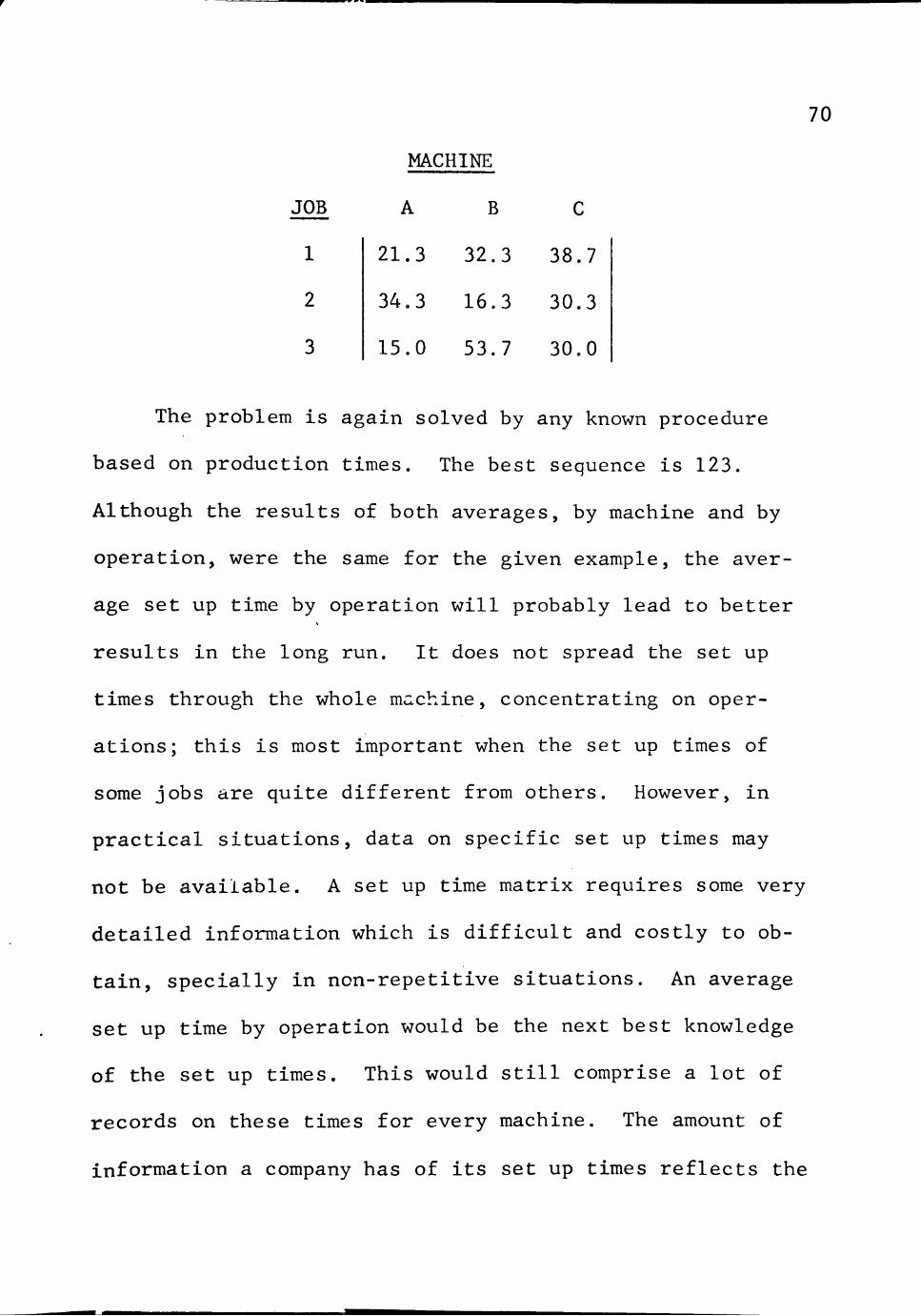
MACHINE
70
JOB A B
1 21.3 32.3 38.7
2 34.3 16.3 30.3
3 15.0 53.7 30.0
The problem is again solved by any known procedure
based on production times. The best sequence is 123.
Although the results of both averages, by machine and by
operation, were the same for the given example, the aver
age set up time by operation will probably lead to better
results in the long run. It does not spread the set up
times through the whole machine, concentrating on oper
ations; this is most important when the set up times of
some jobs are quite different from others. However, in
practical situations, data on specific set up times may
not be available. A set up time matrix requires some very
detailed information which is difficult and costly to ob
tain, specially in non-repetitive situations. An average
set up time by operation would be the next best knowledge
of the set up times. This would still comprise a lot of
records on these times for every machine. The amount of
information a company has of its set up times reflects the

71
importance that it attaches to these times. If the set up
times are considered to be of a relative importance, an
average set up time for each machine is more likely to
exist. This average could, then, be used to solve the
problem.
A Technique Using Set up Time Matrices
The technique is based on a procedure similar to the
one developed by Spencer 14 which solves both flow-shop
and job-shop problems and permits dependence among the
operations. Some modifications have been made to take into
consideration the sequence dependent set up times. The
objective is the minimization of total elapsed time. The
procedure is mainly designed for problems of case 12
(presented in Chapter II), for reasons that will be stated
later in this chapter.
A graphical representation of the problem is used,
similar to the network models analyzed by PERT-CPM tech
niques. The notation to be used in the following analysis
is partially due to Spencer. However, some modifications
were introduced. For example, the nodes are denoted by
job-machine combinations. Also, the letters i, j and k
will refer to jobs, while x, y, z will refer to machines.

72
The GTPO (Graph of Technological Processing Order) combines
the information given by the Processing Time Matrix (P)
and Sequence Matrix (S). Figure 8 presents the GTPO for
the example illustrating case 12 of Chapter II. The graph
utilizes the activity-on-node configuration, i.e., the
activities are graphically represented by the nodes of the
network. The activities are the operations of the jobs on
the machines and, therefore, are defined by the job number,
machine type and processing time. The first and last nodes
of the GTPO are dummy activities introduced to provide
starting (time "0") and finishing (the total elapsed time)
times for the schedule.
Figure 9 shows the possibility of the GTPO to present
dependence requirements. The data is basically the same as
for the example given in Chapter II for the analysis on
minimization of total set up time for the job-shop situa
tion. A dependence requirement has been added: "2B pre
cedes 3B".
The mechanics of the procedure consists of selecting
the appropriate vector from pairs of possible alternative
vectors on each machine. A vector may be defined as an
arrow connecting two nodes in the GTPO. From Figure 9, one
such pair of possible alternative vectors is V(1A,2A) and
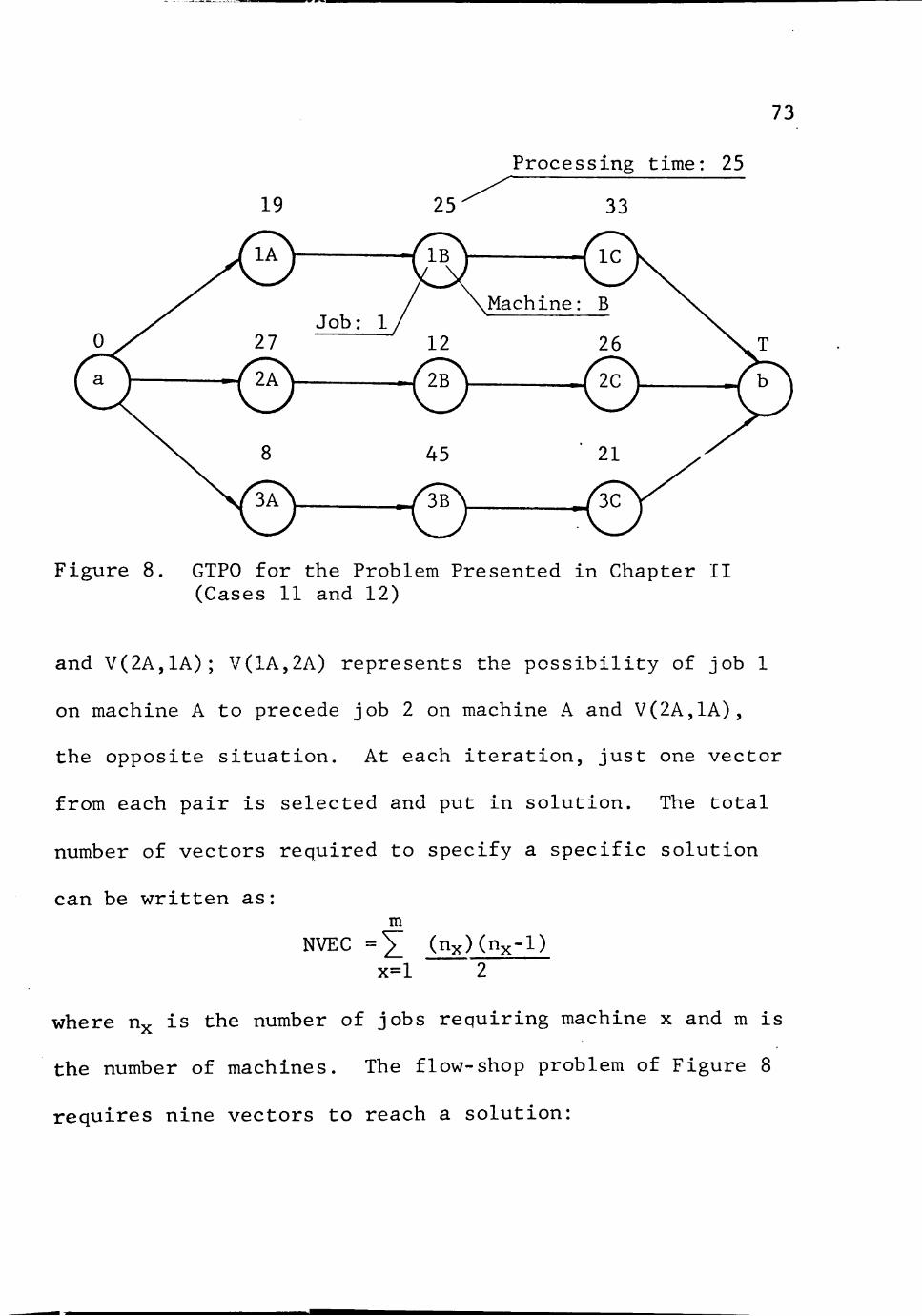
mmmm^maamim ^^m
73
19 25
Processing time: 25
33
Machine: B
Figure 8. GTPO for the Problem Presented in Chapter II (Cases 11 and 12)
and V(2A,1A); V(1A,2A) represents the possibility of job 1
on machine A to precede job 2 on machine A and V(2A,1A),
the opposite situation. At each iteration, just one vector
from each pair is selected and put in solution. The total
number of vectors required to specify a specific solution
can be written as: m
NVEC =5! (nx)(nx-l) x=l 2
where nx is the number of jobs requiring machine x and m is
the number of machines. The flow-shop problem of Figure 8
requires nine vectors to reach a solution:

. K .rtmwwmm\ rm
74
Figure 9: GTPO for a Dependent Job-shop Problem
(A) (B) (C) NVEC = 32^2 ^ 32c2 ^ 32c2 = 9
The problem of Figure 9 also requires nine vectors for
the solution. However, since the precedence requirements
state th.Rt job 2 on machine B should go before job 3 on the
same machine, the vector V(2B,3B) should be placed in solu
tion prior to any other algorithm manipulations. This also
implies the removal of V(3B,2B) from the calculations and
node 2B is said to dominate node 3B.
Description of the Procedure
A standard PERT-CPM forward pass is performed in the
GTPO and the earliest finish time of each node ix is ob-
75
tained, ERLYFT(ix). The latest finish time of the terminal
node b is set equal to its earliest finish time. A standard
PERT-CPM backward pass leads to the latest finish time of
each node ix, LATEFT(ix).
The procedure is based on a minimax criterion in which
one is trying to minimize the maximum possible regret at
any iteration. It does so by introducing into solution the
inverse of the vector with this maximum regret. The
decision criterion for this regret is given by a delta
value, D(ix,jx), which can be defined as: D(ix,jx)=EFTIPJ
(ix,jx) - LATEFT (jx). EFTIPJ(ix,jx) is the earliest finish
time of activity j_X3 given that it is preceded by activity
ix. The expression is defined by:
EFTIPJ(ix,jx) = T(Ox,ix) + EPLYFT(ix) + P(jx)+T(ix,jx)
where: T(Ox,ix) - set up time cf job i if it is the first job to be processed on machine x.
ERLYFT(ix) - earliest finish time of node ix (job i on machine x)
T(ix,jx) - set up time of job j on machine x if its predecessor on this machine is job i.
At each iteration, the deltas for all pairs of vectors
V(ix,jx) and V(jx,ix) are evaluated. The vector correspond
ing to the maximum value of delta is then eliminated from
the calculations and its inverse is placed in solution in
76
the GTPO. After this vector is placed in solution, one
should check for activity dominance in the GTPO. If a
directed path can be traced from any node ix to any node
jx, node ix dominates node jx. Therefore, all vectors
V(ix,jx) should be placed in the GTPO and these vectors,
together with their inverses, V(jx,ix) should be removed
from the calculations of the deltas. This procedure avoids
the possibility of putting in solution any of the infeasible
vectors V(jx,ix) in future iterations through the calcula
tions of the delta values. The PERT-CPM forward and back
ward passes are performed, leading to new values of
earliest and latest finish times which are used for the
next iteration. The procedure is repeated until the number
of vectors in solution equals NVEC; at that point, the
complete schedule has been obtained.
Some comments are now made referring to the calculations
resulting from placing a vector in solution. The PERT-CPM
passes in the original GTPO are performed based only on the
processing times of the operations; no set up times are
included. However, this is not true for the dependent job-
shop in which set up times might exist in the original
GTPO due to the dependency requirements. This case will be
discussed later in further detail. When a vector V(ix,jx)
• '1 »-r-r--i
77
is placed in the GTPO, the set up times associated with
this vector may be included in the calculations, depending
on certain conditions. The two set up times involved are
T(ix,jx) and T(Ox,ix) and they should be studied separately.
T(Ox,ix) is included in node ix if job i may still be
the first job to be processed by machine x. T(Ox,ix) is
removed from EFTIPJ(ix,jx) as soon as one of the following
things occur: 1. a vector V(ix,jx) is placed in solution
and the value T(Ox,ix) is included in the node ix in the
GTPO; 2. a vector V(kx,ix) is placed in solution and job i
can no longer be the first job on machine x, since it is
preceded now by job k. When performing a standard PERT-
CPM forward pass in the GTPO, the following difference
should be calculated: T(Ox,ix) - ERLYFT(iy), given that
job i has to go first on machine y, then on machine x. OnJy
the positive values of this difference are considered for
the forward pass calculations on node ix. If x is the
first machine for job i (node iy=a), then ERLYFT(a)=0 and
the whole value T(Ox,ix) is considered.
T(ix,jx) is to be included in node jx of the GTPO.
However, if in a previous iteration, a vector V(kx,jx) has
been put in solution and its associated set up time T(kx,jx)
has been included in node jx, T(ix,jx) is not considered for

78
the position. The reason is that when a vector V(kx,jx) is
introduced at an early stage in the GTPO, the final
sequence of the jobs on machine x is not yet defined.
Vector V(kx,jx) only means that job k will be processed on
machine x before job j will, and not that j is the immediate
successor of k on that machine. An heuristic rule is then
stated that if a set up time T(kx,jx) has already been
assigned to node jx, this set up time is used in the solu
tion until the final sequence for m.achine x is obtained.
If, in this final solution, a job i immediately precedes
job j, T(ix,jx) is substituted then for T(kx,jx).
Assume that T(ix,jx) is included in the GTPO as a
result of vector V(ix,jx) being placed in solutiofltr When
performing a forward pass, the value T(ix,jx) is considered
for the calculations on node jx if ERLYFT(ix)>ERLYFT(jz),
given that job j has to go first on machine z and then on
machine x. Otherwise, only the positive values of the
difference T(ix,jx) - ERLYFT(jz) - ERLYFT(ix) should be
considered for these calculations.
When performing the PERT-CPM backward pass, the set up
times are only considered for jobs on the same machine. The
reason is that the set up of a job on a specific machine
might be performed while this job is still running on the

79
previous machine.
It was mentioned earlier that the procedure was de
signed for problems of Case 12. Some reasons for this
approach are now given and they are related to the fore
going discussion on how the set up times are placed in the
calculations. When vectors are introduced in the GTPO,
the final sequence of the jobs is not yet known. Set up
times are introduced, then, in a tentative way. Case 12
is not too much affected by the poscible changes that will
occur, since some of the set ups will occur during machine
idle times. In Case 11, however, all set up times con
tribute somewhat to the total elapsed time and, therefore,
any changes in the selected set up times have more relevant
effects in the overall procedure. With these qualifications,
the method could be applied to Caca 11, noting only that
for both forward and backward pass calculations, all the
set up times in the GTPO should be considered.
The following comments relate to dependent job-shop.
The only difference for this case is that the calculations
in the original GTPO might include set up times also. In
the example of Figure 9, the dependence requirement "2B
precedes 3B" is shown in the GTPO by the vector V(2B,3B).
Therefore, the set up times TB(0B,2B) and TB(2B,3B) should
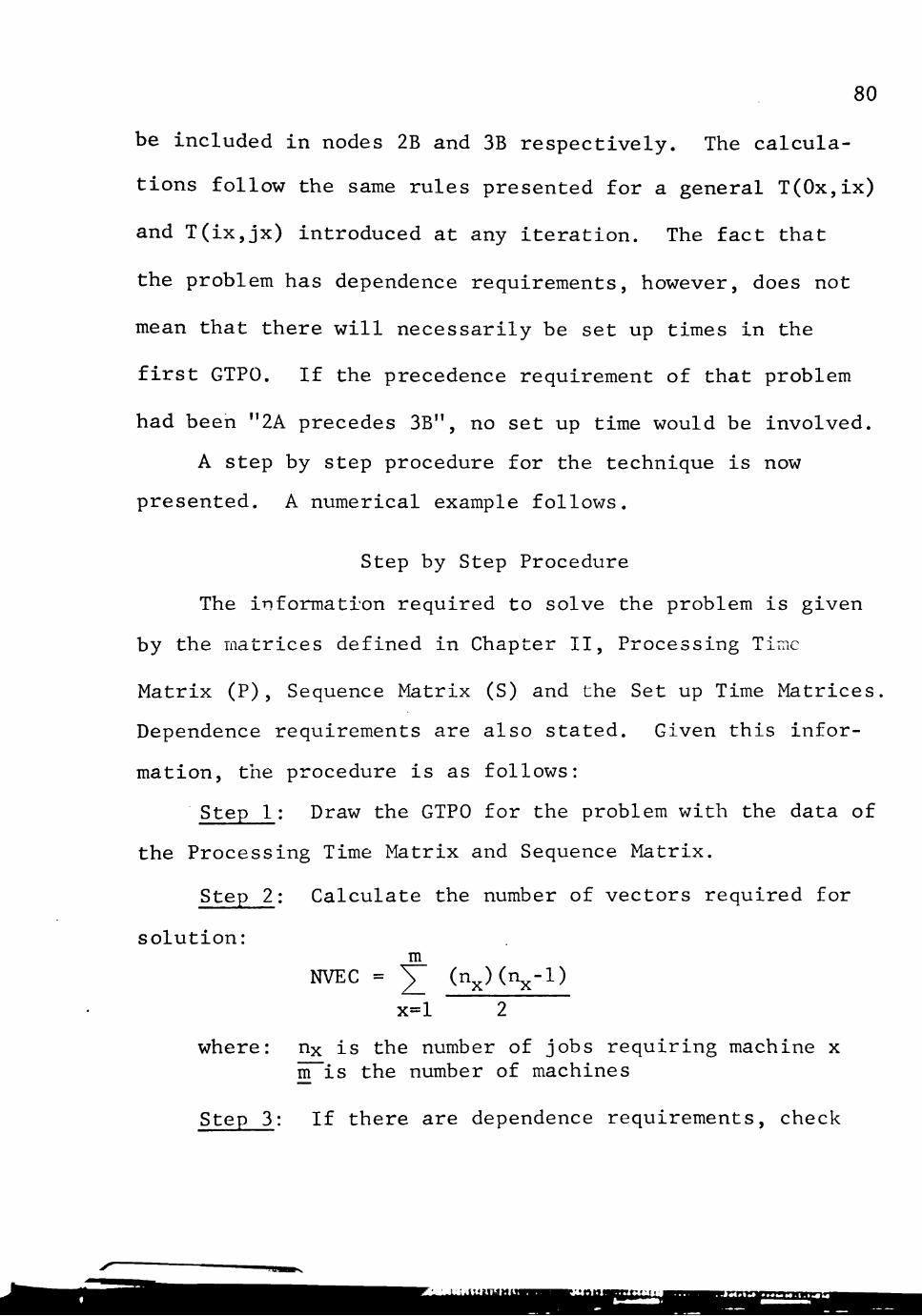
80
be included in nodes 2B and 3B respectively. The calcula
tions follow the same rules presented for a general T(Ox,ix)
and T(ix,jx) introduced at any iteration. The fact that
the problem has dependence requirements, however, does not
mean that there will necessarily be set up times in the
first GTPO. If the precedence requirement of that problem
had been "2A precedes 3B", no set up time would be involved.
A step by step procedure for the technique is now
presented. A numerical example follows.
Step by Step Procedure
The information required to solve the problem is given
by the matrices defined in Chapter II, Processing Time
Matrix (P), Sequence Matrix (S) and the Set up Time Matrices.
Dependence requirements are also stated. Given this infor
mation, the procedure is as follows:
Step 1: Draw the GTPO for the problem with the data of
the Processing Time Matrix and Sequence Matrix.
Step 2
solution:
where:
Calculate the number of vectors required for
m NVEC = Y_ ( x)( " )
x=l 2
nx is the number of jobs requiring machine x nPis the number of machines
Step 3: If there are dependence requirements, check

81
for activity dominance in the GTPO. If a directed path can
be traced from node ix to jx, place the vector V(ix,jx) in
solution. Obtain the values of T(Ox,ix) and T(ix,jx) from
the set up time matrix and include them in nodes ix and jx
respectively. All vectors V(jx,ix) are disregarded from
further calculations. Place all vectors V(ix,jx) in the
solution set and set the number of vectors in solution,
INSOL, equal to the number of vectors V(ix,jx).
Step 4: Perform a standard PERT-CPM forward pass to
obtain ERLYFT(ix) for each node. Three cases may occur,
given that job i has to go first on machine y, then on
maehine x:
1. there is no set up time included in node ij; then:
ERLYFT(ix) = ERLYFT(iy)+P(ix)
2. a set up time T(Ox,ix) has been included in node
ix, then:
ERLYFT(ix)=ERLYFT(iy)+P(ix)-hnax[(T(Ox,ix)-ERLYFT(iy));0]
3. a set up time T(jx,ix) has been included in node ix
(job j precedes job i on machine x), then:
3a. if ERLYFT(jx)>ERLYFT(iy):
ERLYFT(ix)=ERLYFT(jx)+P(ix)+T(jx,ix)
3b. if ERLYFT(jx) <ERLYFT(iy):

_;-^ L_-saf*
82
ERLYFT(ix)=ERLYFT(iy)+P(ix)+ max ([T(jx,ix) -
(ERLYFT(iy)-ERLYFT(jx))] ; o}
Step 5: Set the latest finish time of the terminal
node (b) equal to the earliest finish time of the terminal
node.
Step 6: 1. Perform a standard PERT-GPM backward pass
to obtain LATEFT(ix) for each node. Given that job i has
to go first on machine x, then on machine z and that job i
precedes job k on machine x:
LATEFT(ix)=min[[LATEFT(iz)-P(iz)] ;[LATEFT(kx)-P(kx)-
T(ix,kx)]}
If there is no vector V(ix,kx) in solution,
then: LATEFT(ix)=LATEFT(iz)-P(iz)
2. If the number of vectors in solution,
INSOL, equals NVEC, go to step 9.
Step 7: For all vectors V(ix,jx) and their inverses
V(jx,ix) which have not been placed in solution, obtain
EFTIPJ(ix,jx) the earliest finish time of activity jx,
given that it is preceded by activity ix:
EFTIPJ(ix,jx)=T(0x,ix)4ERLYFT(ix)+P(jx)+T(ix,jx)
Note that the term T(Ox,ix) is excluded from the ex-

83
pression, if: 1. it has already been included in node ix
in a previous iteration; 2. job i can no longer be the
first job on machine x, i.e., a vector V(kx,ix) has been
put in solution in a previous iteration.
Step 8: 1. For all vectors V(ix,jx) and their inverses
V(jx,ix) which have not been placed in solution, calculate
D(ix,jx) through the expression:
D(ix,jx)=EFTIPJ(ix,jx)-LATEFT(jx)
2. Identify the vector V(ix,jx) which has
the maximum D(ix,jx).
3. Place the inverse vector D(jx,ix) in solu
tion and remove both vectors from the calculations of the
deltas. Include the set up time T(Ox,jx) in node jx only
if job j can still be the first job on machine x, i.e.,
there is no vector V(kx,jx) in solution. Include the set
up time T(jx,ix) in node ix only if there is no set up time
already assigned to that node.
4. Place vector V(jx,ix) in the solution set
and increase by one the number of vectors in solution.
5. Check for activity dominance in the GTPO.
If a directed path can be traced from node ix to node jx,
ix dominates jx. Place all vectors V(ix,jx) in solution and

84
remove these vectors and their inverses from the calcula
tions of the deltas. Include the set up time T(Ox,ix) in
node ix only if job i can still be the first job on machine
X. Include the set up time T(ix,jx) in node jx if there is
no set up time already assigned to that node. Place all
vectors V(ix,jx) in the solution set and increase INSOL by
the number of vectors V(ix,jx). Go to step 4.
Step 9: The solution has been obtained. The total
elapsed time for the sequence is the value of ERLYFT(b),
where b is the terminal node of the network. The sequence
of the jobs on the machines is also obtained from the GTPO.
Consider all nodes related to machine x. The node which
has all vectors directed away from itself, but one, repre
sents the first job on machine x; the node with all vectors
directed away from itself, but two, is the second job on
machine x. The analysis is repeated until it reaches the
node with all vectors converging to itself, but one, which
is the last job on this machine.
A Numerical Example
The 3-job, 3-machine flow-shop problem presented in
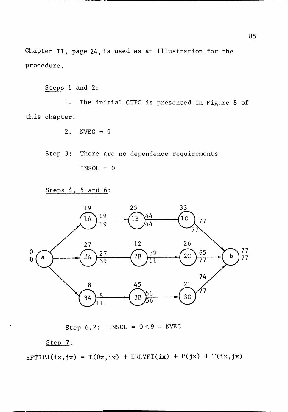
85
Chapter II, page 24,is used as an illustration for the
procedure.
Steps 1 and 2:
1. The initial GTPO is presented in Figure 8 of
this chapter.
2. NVEC = 9
Step 3: There are no dependence requirements
INSOL = 0
Steps 4, 5 and 6
01^—<E)i?—04f
Step 6 . 2 : INSOL = 0 < 9 = NVEC
Step 7:
E F T I P J ( i x , j x ) = T(Ox , ix ) + ERLYFT(ix) + P ( j x ) + T ( i x , j x )
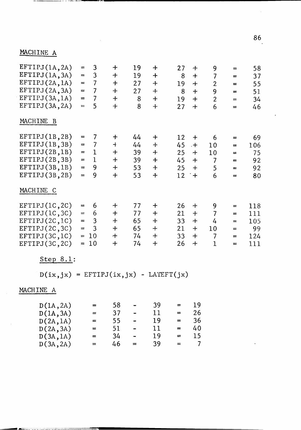
86
MACHINE A
EFTIPJ(1A,2A) EFTIPJ(1A,3A) EFTIPJ(2A,1A) EFTIPJ(2A,3A) EFTIPJ(3A,1A) EFTIPJ(3A,2A)
MACHINE B
EFTIPJ(1B,2B) EFTIPJ(1B,3B) EFTIPJ(2B,1B) EFTIPJ(2B,3B) EFTIPJ(3B,1B) EFTIPJ(3B,2B)
MACHINE C
EFTIPJ(1C,2C) EFTIPJ(1C,3C) EFTIPJ(2C,1C) EFTIPJ(2C,3C) EFTIPJ(3C,1C) EFTIPJ(3C,2C)
Step 8.1:
D(ix,jx)
MACHINE A
= 3 = 3 = 7 = 7 = 7 = 5
= 7 = 7 = 1 = 1 = 9 = 9
= 6 = 6 = 3 = 3 = 10 = 10
+ + + + + +
+ 4 + + + +
+ + + + + +
= EFTIPJ(ix,
19 19 27 27 8 8
44 44 39 39 53 53
77 77 65 65 74 74
,jx) -
+ + + + + +
+ + + + + +
+ + + + + +
LATEFT
27 8 19 8 19 27
12 45 25 45 25 12
26 21 33 21 33 26
"(jx)
+ + + + + +
+ .+ + + +
• +
+ + + + + +
9 7 2 9 2 6
6 10 10 7 5 6
9 7 4 10 7 1
=r
^
zs
z=
=
^
=
:=
=
=
=
^z
=
=
=
=
sr
58 37 55 51 34 46
69 106 75 92 92 80
118 111 105 99 124 111
D(1A,2A) = 58 - 39 = 19 D(1A,3A) = 37 - 11 = 26 D(2A,1A) = 55 - 19 = 36 D(2A,3A) = 51 - 11 = 40 D(3A,1A) = 34 - 19 = 15 D(3A,2A) = 46 = 39 = 7

87
MACHINE B
D(1B,2B) D(1B,3B) D(2B,1B) D(2B,3B) D(3B,1B) D(3B,2B)
MACHINE C
D(1C,2C) D(1C,3C) D(2C,1C) D(2C,3C) D(3C,1C) D(3C,2C)
Step 8.2:
=
=
=
=r
=
=r
=
—
=
=
=
=
69 106 75 92 92 80
118 111 105 99 124 111
51 56 44 56 44 51
77 77 77 77 77 77
18 50
= 31 36 48 29
= 41 = -34
28 22
= 47 34
max D(ix,jx) = D(1B,3B) = 50
inverse vector: V(3B,1B)
Step 8.3:
V(1B,3B) and V(3B,1B) are removed from calculations
V(3B,1B) is placed in solution:
5 — T(3B,1B) 25
9 — T(0B,3B)
mmm
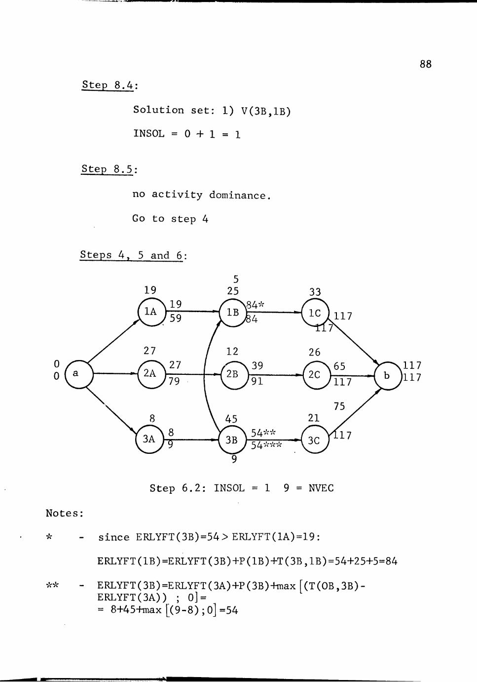
Step 8.4:
Solution set: 1) V(3B,1B)
INSOL = 0 + 1 = 1
Step 8.5:
no activity dominance
Go to step 4
Steps 4 , 5 and 6
88
0 0
N o t e s :
•>v->v
Step 6 . 2 : INSOL = 1 9 = NVEC
s i n c e ERLYFT(3B)=54> ERLYFT(1A)=19:
ERLYFT(lB)=ERLYFT(3B)+P(lB)+T(3B,lB)=54+25+5=84
ERLYFT(3B)=ERLYFT(3A)+P(3B)+max[(T(OB,3B)-ERLYFT(3A)) ; O ] -= 8+45-hnax [(9-8) ; O] =54
*<MM
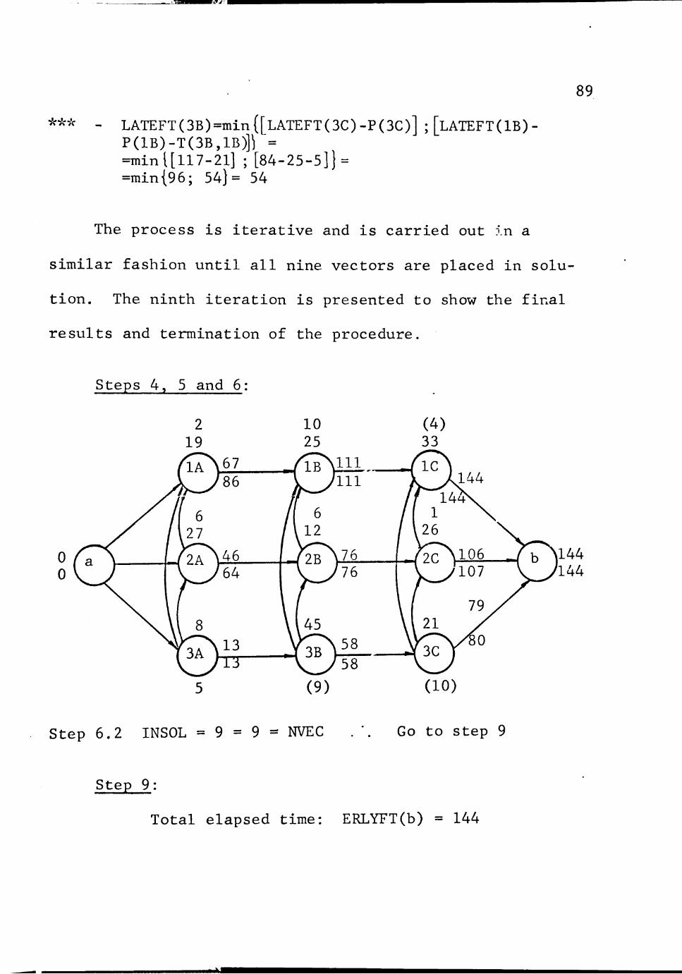
MV
89
•k-k-k _ LATEFT(3B)=min{[LATEFT(3C)-P(3C)] ;[LATEFT(IB) P(lB)-T(3B,lB)]i = =minl[ll7-2l] ; [84-25-5]} = =min{96; 54]= 54
The process is iterative and is carried out in a
similar fashion until all nine vectors are placed in solu
tion. The ninth iteration is presented to show the final
results and termination of the procedure.
Steps 4, 5 and 6:
0 0
Step 6.2 INSOL = 9 = 9 = NVEC Go to step 9
Step 9:
Total elapsed time: ERLYFT(b) = 144
m^M

rj^i
90
Sequence of the jobs on the machines:
Machine Machine Machine
A: B: C:
321 321 321
The above solution is optimal since it is the same as
the optimal solution obtained by enumeration.
Some Final Comments on the Procedures
Some qualifications should be applied to the solution
procedures suggested in this chapter. The average set up
time procedure can be classified as a ^'quick-and dirty"
method to solve the problem as far as the set up times are
concerned. The sequence dependence characteristic of the
set ups is removed and this is obviously a quite severe
handicap for the method. Since averages are substituted
for the true set up times, the procedure should be used
with care. It should probably be used only in situations
in which the set up considerations play a minor role in the
scheduling decision. The average set up time procedure may
also serve in terms of a comparison to other methods that
might be developed, taking into consideration set up times.
While enumeration is generally used for this purpose, the
computational time required becomes prohibitive as the size
of the problem increases. With average set up times and an
91
efficient sequencing method, this computational time is
drastically reduced.
The sequence dependence characteristic of the set up
times is kept in the other procedure suggested. Spencer's
algorithm was selected as a basis for the method for two
main reasons. The first reason is that the algorithm per
mits dependency among the operations. The.second reason
relates to the mechanics of the procedure. At each
iteration, pairs of alternative vectors are studied, for
example V(3A,2A) and V(2A,3A). The set up time matrices
can be considered as formed by similar vectors. For the
specific case of machine A, it shows the set up times
involved if job 2 is to follow job 3 [T(3A,2A)] or if job 3
is to follow job 2 [T(2A,3A)] . This similar configuration
permits these set up times to be included in the calcula
tions at each iteration. However, the general approach
used by Spencer to introduce the vectors in solution pre
sents a disadvantage as far as the set up times are con
cerned. If a vector V(3A,2A) is placed in solution, the
partial sequence 32 on machine A is not yet confirmed.
Therefore, the introduction of the set up time T(3A,2A) is
only a tentative procedure. The extent of this disadvantage
can only be measured when other procedures involving set up
i^mmMmimmsi d ^

92
times are developed. Further research in this area could
lead to a method that defines at each stage partial
sequences for each machine. These sequences should be
definite, so that the exact set up time is used. However,
analyzing each possible alternative partial sequence at
any iteration seems to be a necessary feature of any
procedure dealing with sequence dependent set up times.
raiMiigiiiiiw id if ITU i'I i 'TTiirrinimi

rat
CHAPTER V
CONCLUSIONS AND RECOMMENDATIONS
An overall view on set up times and set up costs in
sequencing problems was presented". The problem was formu
lated and several cases were analyzed. A practical insight
was obtained through a questionnaire which provided the
industry point of view on the matter. Finally some pro
cedures were suggested to solve the problems where the
main concern is the minimization of total elapsed time.
Conclusions
The costs in setting up jobs on machines are due to the
material utilized in the set up and the time (and labor).
If material is the principal factor, the problem is one
of set up costs; if time and labor are predominant, these
costs may be directly proportional to set up times.
When dealing with set up times or costs, several
criteria may be used for schedule evaluation. The analysis
presented here concentrated on such criteria as the minimi
zation of total elapsed time, minimization of set up times
and minimization of set up costs. Problems dealing with
set up times depend on the characteristics of the set ups.
The set up times might be dependent on the sequence or
independent of the sequence. Also, the set up process
might be a function of the machine only or of both job and
• 93
• '-•r-^-rr, ^ - r w . j . TIT-. -"^—~»" ...iVI

94
machine. Four cases were studied, taking into consideration
these factors and the set up times separated from the pro
cessing times. Minimizing total set up costs or total set
up times as sequencing objectives imply the dependence of
these costs or times on the sequence.
The results of a questionnaire utilized in the research
showed some interesting aspects about industrial problems
dealing with set up times and costs. Industry is in
general quite conscious of the matter. However, indica
tions were present suggesting that current industrial pro-
cedures did not include set up conpi.derations as much as
they should.
Meeting of due dates is industry's main concern for
scheduling evaluations. The concepts of customer satis
faction, penalty costs and loss of good will are surely
behind this concern. The other three criteria mentioned
(minimizing total processing time, total set up time and
in-process inventory costs) were assigned almost equal
importance. This shows that total opportunity cost is the
ultimate consideration in most situations.
Time is the main component of the set up costs. Actual
data, however, may not be available. In these cases the

95
set up costs can be considered as a percentage of production
costs. Set up times which are totally sequence dependent
are not a very common occurrence.. Partial dependence (257o
to 757o of the operations with set up times dependent upon
the sequence) was found to be most prevalent.
In industrial practice, an attempt is made to schedule
similar jobs one after the other, whenever this is possible.
Meeting of due dates is again the main reason whenever
these jobs are not scheduled together. Results varied
widely in relation to the extent of similarity.
The small sequencing problem with up to 10 jobs and 10
machines exists in practice. Nevertheless, the companies
surveyed showed that such problems are not as common as the
larger ones. The situations where all machines are of a
different type can also be found in industry. However, the
results of the survey had to be analyzed in perspective.
When the number of machines in a shop is large, one should
not expect all machines to be different. A few identical
machines may exist in some shops; yet these shops would
still be classified as having only one machine of each type.
The proposed methods of solutions presented in Chapter
IV represent only a first step for future research. In this
work these examples were more of an illustrative nature,
^^mmBaz^sKiziSi.i^jsisxiiisi^'.jsiX

96
showing some procedures that could be used as a systematic
approach to solve problems in which set up times receive
consideration.
Recommendations for Further Research
A scheduling procedure with the objective of meeting
due dates while recognizing the existence of set up times
would be very valuable to industrial practices. Research
efforts should be directed toward the development of such
a procedure. Once this is achieved, improvements should
be searched such that the evaluation criterion would
include also other objectives that characterize the prac
tical industrial problem.
Efforts should be made to obtain actual industrial
data. It should be recognized that this is not an easy
task, but such information could direct research to more
practical problems. The concept of similarity of set ups
is one example of what actual data could clarify. The
effects of scheduling similar jobs one after the other in
relation to the overall objective could be studied. Not
only data should be obtained from industry, but also a
closer contact should be established. Large sequencing
problems are solved one way or another by industry. A
careful analysis of these methods and the search for

97
improvements should be attempted. This might provide a
means to overcome the constraint on problem size that has
prevented the use of several theoretical procedures within
industrial applications. The Sequencing Research Group of
Texas Tech University has already made some efforts in
this direction. The thirty-two questionnaires sent to
personal acquaintances of the faculty members of the group
were also used with this idea in mind. An extra page was
included with questions concerning possible future dis
cussions of scheduling problems between members of the
University and these companies.
The cases in which the set up times are not dependent
on the sequence also deserve some further thought. The
research done thus far has included these set up times in
the processing times. However, these set ups might not
depend on the job, i.e., they may be performed while the
specific job is still in process on another machine. In
those cases, it is quite useful to consider the set up
times as a separate entity (case 22 of Chapter II). Pro
cedures that take into consideration this possibility
should be searched.
Finally, research should also be directed to the cases
where only some set up times are sequence dependent. These
n^sM
98
cases in which only a few jobs have their set up times
dependent on the sequence could probably be combined with
job similarity approaches. Situations like this are
common, as reflected in the responses to the questionnaire,
and models to solve these problems should be quite bene
ficial.
I h-Wl r » i w i B a g n i—*»*•ia?^

LIST OF REFERENCES
1. Ackoff, R. L., "Progress in Operations Research" Vol. I, John Wiley & Sons, New York, 1961.
2. Baker, K. R., "Priority Dispatching in the Single Channel Queue with Sequence Dependent Setups", The Journal of Industrial Engineering, Vol. 19, No. 4, 203-206 (1968).
3. Blick, R. G., "Heuristics for Scheduling the General n/m Job-shop Problem", Master's Thesis, Institute of Industrial Administration of Union College, Schenectady, New York, 1969.
4. Conway, R. W. , Maxwell, W. L. and Miller, L. W. , "Theory of Scheduling", Addison-Wesley Publishing Company, Massachusetts, 1967.
5. Gavett, J. W. , "Three Heuristic Rules for Sequencing Jobs to a Single Production Facility", Management Science, Vol. 11, No. 8, B166-B176 (1965).
6. Gupta, J. N. D., "Economic Aspects of Scheduling Theory", Unpubliched Ph. D. Dissertation, Texas Tech University, 1969.
7. Johnson, S. M. , "Optimal Two and Three Stage Production Schedules with Setup Times Included", Naval Research Logistics Quarterly, Vol. 1, 61-68 (1954). r;(
8. Moore, J. M., "An n Job, One Machine Sequencing Algorithm for Minimizing the Number of Late Jobs", Management Science, Vol. 15, No. 1, 102-109 (1968).
9. Naidu, B. R. , "Sensitivity Analysis of Various Criteria for Flow-shop Sequencing with Respect to In-process Inventory Cost", Unpublished Master's Thesis, Texas Tech University, 1969.
10. Sasieni, M. , Yaspan, A. and Friedman, L., "Operations Research - Methods and Problems", John Wiley & Sons, New York, 1966.
99
•M

100
11. Schrage, L., "Solving Resource-Constrained Network Problems by Implicit Enumeration - Nonpreemptive Case", Operations Research, Vol. 18, No. 2, 263-278 (1970).
12. Smith, M. L., "A Critical Analysis of Flow-shop Sequencing", Unpublished Ph. D. Dissertation, Texas Tech University, 1968.
13. Smith, R. D. and Dudek, R. A., "A General Algorithm for Solution of the n-Job, m-Machine Sequencing Problem of the Flow-shop", Operations Research, Vol. 15, No. 1, 71-82 (1967).
14. Spencer, D. L., "An Investigation of the Relationships Between the Sequencing and Scheduling Problems", Unpublished Ph. D. Dissertation, Texas Tech University, 1969.
—fc;^»* »*^miJ m AM

• msm mm i^jtti