Set Predicates in SQL: Enabling Set-Level Comparisons for ... · Set Predicates in SQL: Enabling...

Set Predicates in SQL: Enabling Set-Level

Comparisons for Dynamically Formed GroupsChengkai Li1, Bin He2, Ning Yan1, Muhammad Safiullah3 ∗, Rakesh Ramegowda1

[email protected],{ning.yan,rakesh.ramegowda}@mavs.uta.edu, University of Texas at [email protected], IBM Almaden Research [email protected], Microsoft, Seattle, WA

Abstract— The scalar-level predicates in SQL become in-creasingly inadequate to support a new class of operationsthat require set-level comparison semantics, i.e., comparing agroup of tuples with multiple values. Complex SQL queriescomposed by scalar-level operations are often formed to obtaineven very simple set-level semantics. Such queries are not onlydifficult to write but also challenging for the database engineto optimize, thus can result in costly evaluation. To address thisproblem, this paper proposes to augment SQL with a new typeof predicates, set predicates, to bring out the otherwise obscuresemantics and thus facilitate the direct and efficient support. Weproposed three approaches to answer queries with set predicates:a query rewriting method, an aggregate function-based methodand a bitmap index-based method. Results from comprehensiveexperiments over synthetic and TPC-H data show that the bitmapindex-based approach can significantly outperform the other two.Moreover, we present a histogram-based probabilistic method ofset predicate selectivity estimation, for optimizing queries withmultiple predicates. The experiments also verify the accuracy ofthe estimation and its effectiveness in optimizing queries.

I. INTRODUCTION

With real-world database applications becoming more so-

phisticated, there is a high demand of querying data with the

semantics of set-level comparisons. For instance, a company

may search their resume database for job candidates with a set

of mandatory skills; in business decision making, an executive

may want to find the departments whose monthly average

ratings for customer service in this year have been both good

and bad, i.e., the set of ratings subsumes {excellent, poor};

in online advertisement, a marketing strategist may want to

find all the Websites that publish ads for ING and Emigrant

but not HSBC yet. Since these banks have similar business,

HSBC can be a potential advertiser for those publishers.

In database design, without explicit support, set-valued

attribute is often modeled by a separate table. For example,

a table Resume Skills (id, skill) can be used to connect a

set of skills to job candidates in another table. A GROUP BY

clause can then be used to dynamically group the tuples by id,

with the values on attribute skill in the same group forming a

set. The problem is that current GROUP BY clause can only

do scalar value comparison by an accompanying HAVING

clause. For instance, the SUM/ COUNT/ AVG/ MAX function

will produce a single numeric value which is compared to a

constant or another single aggregate value. A set-level compar-

ison such as the set of skills subsuming {‘Java programming’,

‘Web services’} cannot be accommodated without complex

SQL queries. (Section III-A demonstrates such SQL queries.)

∗ Work performed while Muhammad Safiullah was a student at UTA.

The data modeling literature has long recognized that set-

valued attributes provide a concise and natural way to model

complex data concept such as set [16], [21]. Many DBMSs

nowadays support the definition of attributes involving a set

of values, e.g., nested table in Oracle and SET data type in

MySQL. For example, the “skill” attribute in the resume table

can be defined as a set data type. Set operations can thus be

natively supported on such attributes. Previous research has

extensively studied query processing on set-valued attributes

and set containment joins [7], [19], [11], [12]. Although

set-valued attributes together with set containment joins can

be used to support set-level comparisons, this solution has

inherent limitations: 1) They have to be pre-defined at the

schema definition time; 2) A set can only cover one attribute

and cannot be across multiple attributes.

In real application scenarios, especially OLAP and decision

making, the groups and the corresponding sets are often dy-

namically formed according to the query needs. For instance,

in the aforementioned customer service rating example, the

sets are formed by departments, i.e., the monthly ratings of

each department form a set. In a different query, the sets

may be formed by individual employees. Set-valued attributes,

being pre-defined, cannot support such dynamic set formation.

Moreover, the definition of a set may be over multiple

attributes. Take the example of online advertisement. The

strategist may want to discover the Websites that publish ads

for ING with good profit returns, because those Websites are

already proven to be highly profitable with bank ads. In this

case, the set is defined over both the advertiser and the profitattribute. In many systems a set-valued attribute is only defined

on a single attribute, thus cannot capture the cross-attribute

association in the example. Implementations such as nested

table in Oracle allow sets over multiple attributes but do not

easily support set-level comparisons on such attributes.

Observing the demand for complex and dynamic set-level

comparisons in databases, and limitations of current SQL

language and set-valued attribute, we propose to tackle the

challenge with the introduction of a new concept of set

predicate in HAVING clause. While we elaborate its syntax

in detail in Section II, below we present several examples of

queries with set predicates.

To find the candidates with skills “Java programming” and

“Web services”, the query can be as follows:

SELECT id FROM Resume_Skills GROUP BY id

HAVING SET(skill) CONTAIN {’Java’,’Web services’}

Given the above query, after grouping, a dynamic set of

values on attribute skill is formed for each unique id, and

the groups whose corresponding SET(skill) contain both “Java

programming” and “Web services” are returned.

For the decision making example, suppose we have a

table Ratings(department, avg rating, month, year). The

following query finds the departments whose monthly average

ratings in 2009 have always been poor (assuming ratings are

from 1 to 5). Here CONTAINED BY is used to capture the

set-level condition.

SELECT department FROM Ratings WHERE year = 2009

GROUP BY department

HAVING SET(avg_rating) CONTAINED BY {1,2}

Set predicates can cover multiple attributes. Consider

the online advertisement example. Suppose the table is

Site Statistics(website, advertiser, CTR). The following

query finds the Websites that publish ads for ING with more

than 1% click-through rate (CTR) and do not publish ads for

HSBC yet:

SELECT website FROM Site_Statistics GROUP BY website

HAVING SET(advertiser,CTR) CONTAIN {(’ING’,(0.01,+))}

AND NOT (SET(advertiser) CONTAIN {’HSBC’})

In this example, the first set predicate involves two attributes

and the second set predicate has the negation of CONTAIN.

Note that we use (0.01,+) to represent the partial condition

CTR>0.01.

Without the explicit notion of set predicates, the query

semantics can be captured by using sub-queries connected

by SQL set operations (UNION, INTERSECT, EXCEPT),

in coordination with join and GROUP BY. As Section III-

A will show, such queries can be quite complex for users to

formulate and difficult to optimize for a database engine, thus

can result in unnecessarily costly evaluation. On the contrary,

the proposed construct of set predicate explicitly enables set-

level comparisons. The concise syntax not only makes query

formulation simple but also facilitates native efficient support

of such queries in a query engine.

Our work is mostly related to set-valued attributes and set

containment joins [7], [19], [11], [12]. In comparison, the pro-

posed solution of set predicates has several critical advantages:

(1) Unlike set-valued attributes, which bring significant hassles

in redesigning database storage for the special data type of set,

set predicate requires no change in data representation and

storage engine, therefore can be directly incorporated into any

standard relational databases; (2) Using set predicates, users

can dynamically form set-level comparisons based on their

query needs with no limitation caused by database schema.

On the contrary, for set-valued attributes, sets are statically

pre-defined in the schema design phase. Therefore set-level

comparisons can only be possible on set-valued attributes,

and non-set query conditions could not be easily supported

on set-valued attributes. (3) It allows cross-attribute set-level

comparison, which is not supported by set-valued attributes.

We developed three approaches to implement set predicates:

(1) The query rewriting approach rewrites a SQL query

with set predicates into standard SQL statements. It can be

directly deployed by extending query parser, without changing

query processing engine. However, it can be hard to optimize

complex rewritten queries and thus query performance can

suffer. The resulting query plans could involve multiple sub-

queries with grouping and set operations. (2) The aggregate

function-based approach handles a set predicate like a user-

defined aggregate function [4]. The deployment again would

be simple. Instead of wasteful evaluation of subqueries, only

one pass of table scan could be sufficient. (3) The bitmap

index-based approach evaluates queries with set predicates by

exploiting bitmap index, which is known for its efficient sup-

port of aggregate queries in OLAP and data warehousing. This

approach can significantly outperform the aggregate function-

based approach because it focuses on only tuples from the

groups that satisfy the conditions and only the bitmaps for

relevant columns.

Universal quantification and relational division are power-

ful for analyzing many-to-many relationships and set-valued

attributes [5]. An example universal quantification query is to

find the students that have taken all computer science courses

required to graduate. It is therefore a special type of set

predicates with CONTAIN operator over a set of constants

formed by all the values of an attribute in a table, e.g.,

Courses. By contrast, the proposed set predicate supports

CONTAINED BY and EQUAL, in addition to CONTAIN.

The hash-division algorithm for universal quantification [5]

was shown to be superior than all prior algorithms. Our

aggregate function-based approach is essentially the hash-

division method. However, it handles not only CONTAIN but

also CONTAINED BY and EQUAL. Moreover, we will show

that the bitmap index-based approach significantly outperforms

the aggregate function-based approach.

A query can have multiple set predicates connected by logic

operations (AND, OR, NOT). The straightforward approach to

evaluate such a query is to exhaustively process the predicates

and perform set operations over their resulting groups. It

can be an overkill. A useful optimization rule is to prune

unnecessary set predicates during query evaluation. Given

a query with n conjunctive set predicates, the predicates

can be sequentially evaluated. If no group qualifies after mpredicates are processed, we can terminate query evaluation

without processing the remaining predicates. The number of

“necessary” predicates before we can stop, m, depends on the

evaluation order of predicates. We design a method to select

a good order of predicate evaluation, i.e, an order that results

in a small m, thus a cheap evaluation cost. Our idea is to

evaluate conjunctive (disjunctive) predicates in the ascending

(descending) order of their selectivities, where the selectivity

of a predicate is its number of satisfying groups. We thus

designed a probabilistic approach to estimate set predicate

selectivity by exploiting histograms in databases.

In summary, this paper makes the following contributions:

∙ We proposed to extend SQL with new set predicate for

an important class of analytical queries, which otherwise

would be difficult to write and optimize (Section II).

∙ We designed three query evaluation approaches for set

semester student course grade

Fall09 Mary CS101 4

Fall09 Mary CS102 2

Fall09 Tom CS102 4

Spring10 Tom CS103 3

Fall09 John CS101 4

Fall09 John CS102 4

Spring10 John CS103 3

Table: SC

Fig. 1. A classic student and course example.

predicates, including the baseline query rewriting approach

and aggregate function-based approach (Section III) and the

bitmap index-based approach (Section IV).

∙ We developed a histogram-based probabilistic method of

set predicate selectivity estimation, for optimizing queries

with multiple predicates. Particularly our method determines

the evaluation order of the predicates and stops early without

evaluating unnecessary predicates. (Section V)

∙ We conducted extensive experiments to evaluate and com-

pare the three approaches, over both benchmark and syn-

thetic data. We also investigated the effects of various query

parameters and data characteristics on these approaches.

Moreover, our experiments verify the accuracy and effec-

tiveness of the predicate ordering method. (Section VI)

II. THE SYNTAX OF SET PREDICATES

We extend SQL syntax to support set predicates. Since a set

predicate compares a group of tuples to a set of values, it fits

well into GROUP BY and HAVING clauses. Specifically in the

HAVING clause there is a Boolean expression over multiple

regular aggregate predicates and set predicates, connected by

logic operators ANDs, ORs, and NOTs. The syntax of a set

predicate is:set predicate ::= attribute set set operator constant values

attribute set ::= SET(v1, ..., vm)

set operator ::= CONTAIN ∣ CONTAINED BY ∣ EQUAL

constant values ::= {(v11 , ..., v1m), ..., (vn1 , ..., vnm)},

where vji ∈ Dom(vi), i.e., each vji can be a value (integer,

floating point number, string, etc.) in the domain of attribute

vi. Succinctly we denote a set predicate by (v1, ..., vm) op

{(v11 , ..., v1m), ..., (vn1 , ..., vnm)}, where op can be ⊇, ⊆, and

=, corresponding to the set operator CONTAIN, CONTAINED

BY, and EQUAL, respectively.

We further extend relational algebra to include set predicates

for concise query representation. Given relation R, the group-

ing and aggregation is represented by the following operator 1:

G,AC(R)

where G is a set of grouping attributes, A is a set of

aggregates (e.g., COUNT(*)), and C is a Boolean expres-

sion over set predicates and conditions on aggregates (e.g.,

AVG(grade)>3), which may overlap with the aggregates in

A. Note that relation R can be the result of a query.

We now provide examples of SQL queries with set predi-

cates, over the classic student-course table (Figure 1).

1Note that there is no agreed-upon notation for grouping and aggregationin relational algebra.

Single-Predicate Set Operation: The following query Q1:

studentcourse⊇{‘CS101’,‘CS102’}(SC) identifies the students who

took both CS101 and CS102. 2 The results are Mary and John.

The keyword CONTAIN represents a superset relationship,

i.e., the set variable SET(course) is a superset of {‘CS101’,

‘CS102’}.Q1: SELECT student FROM SC GROUP BY student

HAVING SET(course) CONTAIN {’CS101’, ’CS102’}

A more general query can include regular WHERE clause

and conditions on aggregate functions in HAVING. In the

following Q2: student,COUNT (∗) course ⊇ {‘CS101’, ‘CS102’} &&

AVG(grade) > 3.5 (�semester=′Fall09′ (SC)), we look for students

with average grade higher than 3.5 in FALL09 and have taken

both CS101 and CS102 in that semester. It also returns the

number of courses they took in that semester.Q2: SELECT student, COUNT(*) FROM SC

WHERE semester = ’Fall09’ GROUP BY student

HAVING SET(course) CONTAIN {’CS101’, ’CS102’}

AND AVG(grade)>3.5

We use CONTAINED BY for the reverse of CONTAIN,

i.e., the subset relationship. The following query selects all

the students whose grades are never below 3. The results are

Tom and John. Note that set predicates follow set semantics

instead of bag semantics, therefore John’s grades, {4,4,3}, is

subsumed by {4,3}.Q3: SELECT student FROM SC GROUP BY student

HAVING SET(grade) CONTAINED BY {4, 3}

To select the students that have only taken CS101 and

CS102, the following query uses EQUAL to represent the

equal relationship in set theory. Its result contains only Mary.Q4: SELECT student FROM SC GROUP BY student

HAVING SET(course) EQUAL {’CS101’, ’CS102’}

Multi-Predicate Set Operation: A query with multiple

set predicates can be supported by using Boolean oper-

ators, i.e., AND, OR, and NOT. For instance, to iden-

tify all the students whose grades are never below 3,

except those who took both CS101 and CS102, we

can use NOT (SET(course) CONTAIN {’CS101’, ’CS102’})

AND SET(grade) CONTAINED BY {4,3}.

Multi-Attribute Set Operation: The query syntax also allows

cross-attribute comparisons, e.g., we use SET(course,grade)

CONTAIN {(’CS101’,4),(’CS102’,2)} for all the students

who received grade 4 in CS101 but 2 in CS102.

Constant Values from Subqueries and in Ranges: The

constant values in the set predicate can be from the result

of a subquery, e.g., SET(course) CONTAIN (SELECT course

FROM core course). Moreover, for data types such as numeric

attributes and dates, the constant value can be a range. One

example is the online advertisement query in Section I.

III. TWO BASELINE APPROACHES

A. Query Rewriting Approach

One easy-to-deploy approach is to rewrite queries with set

predicates into standard SQL queries. Due to space limitations,

we only provide a summary here. Details of the formal and

2To be rigorous, it should be (course) ⊇ {(‘CS101’), (‘CS102’)}, basedon the aforementioned syntax.

SELECT sum(a)FROM R,

Seq Scan

39.063 ms

368.190 ms

FROM R,( SELECT gFROM REXCEPT( SELECT g FROM RWHERE v <> 1 AND v <> 2 AND v <> 3)

) AS TMPWHERE R.g = TMP.g

Seq Scan

R

WHERE R.g = TMP.g GROUP BY R.g

Hash Join

Hash Aggregate

402.067 ms

402.468 ms

Seq Scan

Except

Project &

Sort on g

Append

Seq Scan

R

39.063 ms

161.989 ms

328.102 ms

368.190 ms 14.791 ms

Filter38.950 ms

Seq Scan

Seq Scan

R38.950 ms

Filter

v<> 1 && v<>2 && v<>3

Fig. 2. Rewritten query and query plan for g,SUM(a)v⊆{1,2,3}(R) over100K tuples, 1K groups, and 10 satisfying groups.

systematic rewriting procedure and examples can be found

in Appendix I. The basic idea is to rewrite a set predicate

by using SQL set operations. A CONTAIN predicate with

m constant values can be rewritten using m-1 INTERSECT

operations. A CONTAINED BY predicate can be rewritten by

using EXCEPT. The rewriting of EQUAL predicates naturally

combines that of CONTAIN and CONTAINED BY. To rewrite

more complex queries with multiple predicates, we use the

rewriting of individual predicates as the building blocks and

connect them together by their logical relationships. If the

SELECT clause in the query contains aggregate values, the

rewritten query needs to be joined with the original table on

the grouping attributes.

The advantage of the rewriting approach is that it requires

no change inside query engine. However, the rewritten query

can be complex thus difficult to optimize for a database engine,

resulting in over-costly evaluation plan. While more details on

our experiments with this approach are in Section VI, below

we give an example to just get a sense of the issues.

Figure 2 illustrates a PostgreSQL query plan for the rewrit-

ten query of g,SUM(a) v ⊆ {1,2,3}(R) over a 100K-tuple

table R with 1K groups on g, resulting in 10 qualifying groups.

The plan is hand-picked and the most efficient among the ones

we have investigated. It also shows the time spent on each

operator (which recursively includes the time spent on all the

operators in the sub-plan tree rooted at the given operator, due

to the effect of the iterators’ GetNext() interfaces.) The real

PostgreSQL plan had more detailed operators. We combine

them and give the combined operators more intuitive names,

for the ease of presentation.

Figure 2 shows, given the simple original query, the rewrit-

ten query involves a set difference operation (Except) and a

join. The set difference is between R itself (100K tuples) and

a subset of R (98998 tuples that do not have 1, 2, or 3 on

attribute v). Both sets are large, making the Except operator

cost much more than a simple sequential scan.

B. Aggregate Function-Based Approach

The example at the end of Section III-A indicates that

the rewritten query obscures the semantics of set predicate,

making it very difficult for the query optimizer to optimize.

With the new syntax in Section II bringing forward the

Algorithm 1 Aggregate Function-Based Approach

Input: Table R(g, a, v), Query Q = g,⊕a v op {v1, ..., vn}(R)Output: Qualifying groups g and their aggregate values ⊕a

/* g: grouping attribute; a: aggregate attribute; v: attribute in setpredicate; A: hash table for aggregate values; M : hash table forconstant value masks; G: hash table for Boolean indicators ofqualifying groups */

1: while r(g,a,v)⇐GETNEXT( ) != End of Table do2: if group g is not in hash table A,M ,G then3: M [g] ⇐ 0; G[g]⇐(op ∈ {⊆,=}); also initialize A[g]

according to the aggregate function.

4: /* Aggregate the value a for group g. */5: A[g] ⇐ A[g]⊕ a6: /* In M [g], set the mask for the jth constant value. */7: if (M [g] != 2n − 1)&&((op is ⊇)∣∣((op is =)&&G[g])) then8: if v == vj for some j then9: M [g] ⇐ M [g] ∣ 2j−1

10: /* For ⊆, =, if v /∈ {v1, ..., vn}, g does not qualify. */11: if G[g] && (op ∈ {⊆,=}) && (v ∕= vj for any j) then12: G[g] ⇐ False

13: /* Output qualifying groups and their aggregates. */14: for every group g in hash table M do15: if (op is =) && (M [g] != 2n − 1) then G[g] ⇐ False16: if G[g] then print (g, A[g])

semantics explicitly, a set predicate-aware query plan could

potentially be much more efficient by just scanning the table

and processing the tuples sequentially. The key to such a direct

approach seems to be processing the grouping and the set-

level comparison together, through a one-pass iteration of the

tuples, instead of using set operations and joins. In light of

this idea, we design another baseline approach, the aggregate

function-based method, that handles set predicates as user-

defined aggregate functions [4]. The outline of the method is

shown in Algorithm 1.

For the ease of presentation, we first assume the simplest

query, g,⊕a v op {v1, ..., vn}(R), i.e., a query with one

grouping attribute (g), one aggregate for output (⊕a), and

one set predicate defined by a set operator (⊇, ⊆, or =) over

a single attribute (v). Algorithm 1 uses the standard iterator

interface GetNext() to go thorough the tuples in R, may it be

from a sequential scan over table R or the sub-plan over sub-

query R. Follow the common implementation of user-defined

aggregate functions in database systems, e.g., PostgreSQL, a

set predicate is treated as an aggregate function, defined by

an initial state (line 3), a state transition function (line 4-

12), and a final calculation function (line 15-16). The hash

table M maintains a mask value for each unique group. The

bits in the binary representation of a mask value indicate

which of the constant values v1, ..., vn in the set predicate

are contained in the corresponding group. (The ∣ in line

9 is the bitwise OR operator instead of logical OR ∣∣.) If

the mask value equals 2n − 1, where n is the number of

the constant values, the corresponding group contains all the

constant values. The algorithm sketch covers the three kinds

of set operators, CONTAIN, CONTAINED BY, and EQUAL.

The above algorithm can be conveniently extended for gen-

eral queries with set predicates. Such queries can be denoted

by G,AC(R), as introduced in Section II. The aggregates that

are in A (to appear in the SELECT clause) or in the conditions

in C (to appear in HAVING) can be evaluated simultaneously

with set predicates. The aggregate ⊕a in Algorithm 1 already

demonstrates that. 3

We have assumed that one-pass algorithm is sufficient,

i.e., memory is available for storing the hash tables for all

the groups. If the required memory size is too large to be

affordable, we can adopt the standard two-pass hash-based or

sort-based aggregation method in DBMSs. The table is sorted

or partitioned by a hash function so that the tuples in the

same group can be loaded into memory and aggregations over

different groups can be handled independently.

IV. BITMAP INDEX-BASED APPRAOCH

Our third approach is based on bitmap index [14], [15].

Given a bitmap index on an attribute, there exists a bitmap (a

vector of bits) for each unique attribute value. The length of

the vector equals the number of tuples in the indexed relation.

In the vector for value x of attribute v, its ith bit is set to

1, when and only when the value of v on the ith tuple is x,

otherwise 0. With bitmap indices, complex selection queries

can be efficiently answered by bitwise operations (AND (&),

OR(∣), XOR(ˆ), and NOT(∼)) over the bit vectors. Moreover,

bitmap indices enable efficient computation of aggregates such

as SUM and COUNT [15].

The idea of using bitmap index is in line with the aforemen-

tioned intuition of processing set-level comparison by a one-

pass iteration of the tuples (in this case, their corresponding

bits in the bit vectors). On this aspect, it shares the same

advantage as the aggregate function-based approach. However,

this method also leverages the distinguishing characteristics

of bitmap index, making it potentially more efficient than the

aggregate function-based approach. Specifically, using bitmap

index to process set predicates brings several advantages.

(1) We only need to access the bitmap indexes on columns

involved in the query, therefore the query performance is

independent of the width of the underlying table. (2) The data

structure of bit vector is efficient for basic operations such

as membership checking (for matching constant values in set

predicates). Bitmap index gives us the ability to skip tuples

when they are irrelevant. Given a bit vector, if there are chunks

of 0s, they can be skipped together due to effective encoding of

the vector. (3) The simple data format and bitmap operations

make it convenient to integrate the various operations in a

query, including the dynamic grouping of tuples and the set-

level comparisons of values. It also enables efficient and

seamless integration with conventional operations such as

selections, joins, and aggregates. (4) It allows straightforward

extensions to handle features that could be complicated, such

as multi-attribute set predicates, multi-attribute grouping, and

multiple set predicates.

As an efficient index for decision support queries, bitmap

index has gained broad interests. Although bitmap index is

3Note that line 5 of Algorithm 1 only shows the state transition of ⊕. Theinitialization and final calculation steps are omitted.

arguably not as standard as some other index structures such

as B+ tree, it is widely adopted in DBMSs. Nowadays, bitmap

index is supported in major commercial database systems

(e.g, Oracle, SQL Server), and it is often the default (or

only) index option in column-oriented database systems (e.g.,

Vertica, C-Store [22], LucidDB), especially for applications

with read-mostly or append-only data, such as OLAP and

data warehouses. The state-of-the-art developments of bitmap

compression methods [25], [1], [9] and encoding strategies [2],

[26], [15] have substantially broaden the applicability of

bitmap index. Today’s bitmap index can be applied on all types

of attributes (e.g., high-cardinality categorical attributes [24],

[25], numeric attributes [24], [15] and text attributes [20]).

Studies show that compressed bitmap index occupies less

space than the raw data [25], [1] and provides better query

performance for equality query [25], range query [24], and

aggregation [15]. Bitmap index has also been used for indexing

set-valued attributes [13]. A vector represents a value of a set-

valued attribute, where each bit in the vector corresponds to a

distinct member of the set.

A. Basic Set Predicate Queries

In presenting the bitmap index-based approach, we first fo-

cus on the simplest case– a query with only one set predicate,

g,⊕a v op {v1, ..., vn}(R), where op can be any of the set

operators ⊇, ⊆, and =. Section IV-B discusses the extension

to more general queries.

One particular type of bitmap index that we use is bit-

sliced index (BSI) [20]. Given a numeric attribute on integers

or floating-point numbers, BSI directly captures the binary

representations of attribute values. The tuples’ values on an

attributes are represented in binary format and kept in sbit vectors (i.e., slices), which represent 2s different values.

Categorial attributes can be also indexed by BSI, with a

mapping from unique categorical values to integer numbers.

The approach requires that bit-sliced indexes are built on g(BSI(g)) and a (BSI(a)), respectively, and there is a bitmap

index on v (BI(v)), which can be a BSI or any regular bitmap

index. With the aforementioned effective compression and

encoding schemes, it is affordable to build bitmap indexes

on many attributes. Index selection based on query workload

could allow a system to selectively create indexes on attributes

that are more likely to be used in queries. Some systems (e.g.,

DB2, PostgreSQL) build bitmap indxes on the fly when the

query optimizer determines they are beneficial. We do not

consider such scenario and we focus on bitmap indexes that

are built before query time.

Note that the algorithm presented below will also work

if we have other types of bitmap indexes on g and a, with

modifications that we omit. The advantage of BSI is that it

indexes high-cardinality attributes with small number of bit

vectors, thus improves the query performance if the grouping

or aggregation is on such high-cardinality attribute.

Example 1: Given the data in Figure 1 and query

student,AV G(grade) course op {‘CS101’,‘CS102’}(SC), Figure 3

shows the bitmap indexes on g (student), v(course), and

Algorithm 2 Basic Set Operation (⊇, ⊆, =)

Input: Table R(g, a, v) with t tuples;Query Q = g,⊕a v op {v1, ..., vn}(R);bit-sliced index BSI(g), BSI(a), and bitmap index BI(v).

Output: Qualifying groups g and their aggregate values ⊕a/* gID: array of size t, storing the group ID of each tuple *//* A: hash table for aggregate values *//* M : hash table for constant value masks *//* G: hash table for Boolean indicators of qualifying groups *//* Step 1. get the vector for each constant in the predicate */

1: for each vj do2: vecvj ⇐ QUERYBI (BI(v), vj )

/* Step 2. get the group ID for each tuple */3: Initialize gID to all zero4: for each bit slice Bi in BSI(g), i from 0 to s-1 do5: for each set bit bk in bit vector Bi do6: gID[k] ⇐ gID[k] + 2i

7: for each k from 0 to t-1 do8: if group gID[k] is not in hash table A,M ,G then9: M [gID[k]]⇐0; also initialize A[gID[k]] according to

the aggregate function.10: G[gID[k]]⇐ (op is ⊆)

/* Step 3. find qualifying groups */11: if op ∈ {⊇, =} then12: for each bit vector vecvj do13: for each set bit bk in vecvj do14: M [gID[k]] ⇐ M [gID[k]] ∣ 2j−1

15: for each group g in hash table M do16: if M [g] == 2n − 1 then G[g] ⇐ True

17: if op ∈ {⊆, =} then18: for each set bit bk in ∼(vecv1 ∣ ... ∣ vecvn ) do19: G[gID[k]] ⇐ False

/* Step 4. aggregate the values of a for qualifying groups */20: for each k from 0 to t-1 do21: if G[gID[k]] then22: agg ⇐ 023: for each slice Bi in BSI(a) do24: if bk is set in bit vector Bi then agg ⇐ agg + 2i

25: A[gID[k]] ⇐ A[gID[k]]⊕ agg

26: for every group g in hash table M do27: if G[g] then print (g, A[g])

a(grade). BSI(student) has two slices. For instance, the fourth

bits in B1 and B0 of BSI(student) are 0 and 1, respectively.

Thus the fourth tuple has value 1 on attribute student, which

represents ‘Tom’ according to the mapping from the original

values to numbers. There is also a BSI(grade) on grade. The

bitmap index on course is not a BSI, but a regular one where

each unique attribute value has a corresponding bit vector. For

instance, the bit vector BCS101 is 1000100, indicating that the

1st and the 5th tuples have ‘CS101’ as the value of course.□

The outline of the algorithm for processing the query is in

Algorithm 2. It takes four steps. Step 1 is to get the tuples

having values v1, ..., vn on attribute v. Given value vj , the

function QueryBI in line 2 queries the bitmap index on v,

BI(v), and obtains a bit vector vecvj , where the kth bit is set

(i.e., having value 1) if the kth tuple of R has value vj on

attribute v. Note that this is the basic functionality supported

by every bitmap index.

Step 2 is to get the group IDs, i.e., the values of attribute

Mapping from values in student to numbers:

Mary=>0;Tom=>1;John=>2

student course grade

B1 B0 BCS101 BCS102 BCS103 B2 B1 B0

0 0 1 0 0 1 0 0

0 0 0 1 0 0 1 0

0 1 0 1 0 1 0 0

0 1 0 0 1 0 1 1

1 0 1 0 0 1 0 0

1 0 0 1 0 1 0 0

1 0 0 0 1 0 1 1

Fig. 3. Bitmap indexes for the data in Figure 1.

g, for the tuples in R, by querying BSI(g). The group IDs

are calculated by iterating through the slices of BSI(g) and

summing up the corresponding values for tuples with bits set

in these vectors.

Step 3 gets the groups that satisfy the set predicate, based

on the vectors from Step 1. The algorithm outline is applicable

to any of the three set operators, although the details differ.

Below we will introduce Step 3 for different operators.

Step 4 gets the aggregates for the qualifying groups from

Step 3 by using BSI(a). It is pretty similar to how Step

2 and Step 3 are accomplished. It aggregates the value of

attribute a from each tuple into its corresponding group if it

is a qualifying group. The value of attribute a for the kth

tuple is obtained by assembling the values 2i−1 from the

slices Bi when their kth bits are set. The algorithm outline

checks all the bit slices for each k. Note that this can be

efficiently implemented by iterating through the bits (k from

0 to t− 1) of the slices simultaneously. We do not show such

implementation details in the algorithm outline, for simplicity.

CONTAIN (⊇): In Step 3, a hash table M maintains a mask

value M [g] for each group g. The mask value has n bits,

corresponding to the n constant values (v1, ..., vn) in the set

predicate. A bit is set to 1 if there exists at least one tuple in

group g that has the corresponding constant value on attribute

v. Therefore for each set bit bk in vector vecvj , the jth bit

of M [gID[k]] will be set (line 14 of Algorithm 2). (The ∣ in

line 14 is the bitwise OR operator instead of logical OR ∣∣.)Therefore if M [g] equals 2n−1 at the end, i.e., all the n bits

are set, the group g contains tuples matching every constant

value in the set predicate, thus satisfies the query (line 16). We

use another hash table G to record the Boolean indicators of

qualifying groups. The values in G were initialized to Truefor every group if the operator is ⊆ (line 10), otherwise False.

CONTAINED BY (⊆): If the set operator is ⊆, Step 3 will

not use hash table M . Instead, for a set bit bk in ∼(vecv1 ∣ ...

∣ vecvn ) (i.e., the kth tuple does not match any constant vj ),

the corresponding group gID[k] could not satisfy the query

condition and thus will immediately be disqualified (line 19).

EQUAL (=): Step 3 for EQUAL (=) is naturally a combina-

tion of that for ⊇ and ⊆. It first marks a group as qualifying

if ⊇ is satisfied (line 16), then disqualifies group gID[k] if ⊆is not satisfied (line 19).

Example 2: Suppose the query is student,AV G(grade) course= {‘CS101’,‘CS102’}(SC), using the bitmap indexes in Fig-

ure 3. After the 1st bit of vecCS101 (i.e., v1=‘CS101’) is

encountered in line 13, M [0]=20=1 since the 1st tuple in SCbelongs to group 0 (Mary). After the 2nd bit of vecCS102

(the 1st set bit) is encountered, M [0]=1∣21=3. Therefore G[0]becomes True. Similarly G[2] (for John) becomes Trueafter the 6th bit of vecCS102 is encountered. However, since

∼(vecCS101 ∣ vecCS102) is 0001001, G[2] becomes Falseafter the last bit of 0001001 is encountered in line 18 (i.e.,

John has an extra course ‘CS103’). □

B. General Queries with Set Predicates

A general query G,AC(R) may use multiple grouping

attributes and multiple set predicates, and each predicate may

be defined on multiple attributes. Below we discuss how to

extend the method in Section IV-A for such general queries.

A query may also return multiple aggregates, e.g., g,⊕1a,⊕2b vop {v1, ..., vn}(R), which can be simply handled by repeating

the Step 4 of Algorithm 2 for multiple aggregates. Thus such

case will not be further discussed.

Multi-Attribute Grouping: Given a query with multiple

grouping attributes, g1,...gl,A C(R), we can treat the grouping

attributes as a single combined attribute g. That is, the con-

catenation of the bit slices of BSI(g1), ..., BSI(gl) becomes

the bit slices of BSI(g). For example, given Figure 3, if

the grouping condition is GROUP BY student,grade, the

BSI of the conceptual combined attribute g has 5 slices,

which are B1(student), B0(student), B2(grade), B1(grade),

and B0(grade). Thus the binary value of the combined group

g of the first tuple is 00100.

Multi-Attribute Set Predicates: For a query with multiple

attributes in defining the set predicate, G,A (v1, ..., vm) op

{(v11 , ..., v1m), ..., (vn1 , ..., vnm)}(R), we again can view the

concatenation of v1, ..., vm as a combined attribute v. To

replace the Step 1 of Algorithm 2, we first obtain the vectors

vecvj1

, ..., vecvjm

by querying BI(v1), ..., BI(vm). Then the

intersection (bitwise AND) of these vectors, vecvj = vecvj1

&... & vec

vjm

, gives us the tuples that match the multi-attribute

constant (vj1, ..., vjm).

Multi-Predicate Set Operation: Given a query with multiple

set predicates, the straightforward approach is to evaluate

the individual predicates independently to obtain the qual-

ifying groups for each predicate. Then we can follow the

logic operations between the predicates (AND, OR, NOT)

to perform the intersection, union, and difference operations

over the qualifying groups. Different orders of evaluating the

predicates can lead to different evaluation costs, due to their

different “selectivities”, i.e., the number of qualifying groups.

We discuss this query optimization issue in Section V.

In a general query, the HAVING clause may also

have conditions over regular aggregate expressions, e.g.,

AVG(grade)>3.5 in Q2. Following the same way as the

aggregates in SELECT clause are calculated, in Step 4 of

Algorithm 2, we can obtain the multiple aggregates for each

group and remove a group from the result if the condition over

an aggregate is not satisfied.

Integration and Interaction with Conventional SQL Op-

erations: In a general query G,AC(R), relation R could be

the result of other operations such as selections and joins.

Logical bit vector operations allow us to integrate the bitmap

index-based method for set predicates with the bitmap index-

based solutions for selection conditions [2], [26], [15] and

join queries [14]. That is, only bitmap-index on the under-

lying tables (instead of the dynamic result R) is required.

In Section VI-B we present the experimental results of such

general queries on TPC-H data [23]. The detailed method of

dealing with general queries is in Appendix II. The techniques

are similar to those in [10], where bitmap index is used to

incorporate clustering with ranking, selections, and joins.

V. OPTIMIZING QUERIES WITH MULTIPLE SET

PREDICATES: SELECTIVITY ESTIMATION BY HISTOGRAM

The straightforward approach to evaluate a query with mul-

tiple set predicates is to exhaustively process the predicates and

perform set operations over their resulting groups. However,

this approach can be an overkill. An obvious example is query

g,⊕a v⊇{1}(R) AND v⊇{1, 2}(R). The constant set of the

first predicate is a subset of the second constant set. Evaluating

the first predicate is unnecessary because its satisfying groups

are always a superset of the second predicate’s satisfying

groups. Similarly the second predicate can be pruned if the

query uses OR instead of AND. Another example is g,⊕a

v⊆{1}(R) AND v⊇{2, 3}(R). The two constant sets are

disjoint. Without evaluating either predicate, we can safely

report empty result. These examples show that, given multiple

predicates on the same set of attributes, we can eliminate the

evaluation of redundant or contradicting predicates based on

set-containment or mutual-exclusion between the predicates’

constant sets. We do not further elaborate on such logical

optimization since query minimization and equivalence [3] has

been a well-established database topic.

The above optimization is applied without evaluating predi-

cates because it is based on algebraic equivalences that are

data-independent. A more general optimization is to prune

unnecessary set predicates during query evaluation. The idea

is as follows. Suppose a query has conjunctive set predicates

p1, ..., pn. We evaluate the predicates sequentially, obtain the

satisfying groups for each predicate, and thus obtain the groups

that satisfy all the evaluated predicates so far. If no satisfying

group is left after p1, ..., pm (m<n) are processed, we termi-

nate the query evaluation, without processing the remaining

predicates. Similarly, if the predicates are disjunctive, we

stop the evaluation if all the groups satisfy at least one of

p1, ..., pm. In general the smaller the value m is, the cheaper

the evaluation cost is. (The cost difference between predicates

will also have an impact. We are assuming equal predicate

cost for simplicity. Optimization by predicate-specific cost

estimation warrants further study.)

The number of “necessary” predicates before we can stop,

m, depends on the evaluation order of predicates. For instance,

suppose the query has three conjunctive predicates p1, p2, p3,

which are satisfied by 10%, 50%, and 90% of the groups,

respectively. Consider two different orders of predicate eval-

uation, p1p2p3 and p3p2p1. The former order may have a

much larger chance than the latter order to terminate after

2 predicates, i.e., reaching zero satisfying groups after p1and p2 are evaluated. Therefore different predicate evaluation

orders can potentially result in much different costs. Given npredicates, by randomly selecting an order out of n! possible

orders, the chance of hitting a good efficient one is slim, not to

mention the optimal evaluation plan. This is a typical scenario

in query optimization. Our goal is thus to design a method to

select a good order, i.e, an order that results in a small m.

Such good order hinges on the “selectivities” of predi-

cates. Suppose a query has predicates p1,...,pm, which are in

either conjunctive form (connected by AND) or disjunctive

form (OR). Each predicate can have a preceding NOT.4 Our

query optimization rule is to evaluate conjunctive (disjunctive)

predicates in the ascending (descending) order of selectivities,

where the selectivity of a predicate is its number of satisfying

groups. Therefore the key challenge in optimizing multi-

predicate queries becomes estimating predicate selectivity.

To optimize an SQL query with multiple selection pred-

icates that have different selectivities and costs, the idea of

predicate migration [6] is to evaluate the most selective and

cheapest predicates first. The intuition of our method is similar

to that. However, we focus on set predicates, instead of the

tuple-wise selection predicates studied in [6]. Consequently the

concept of “selectivity” in our setting stands for the number

of satisfying groups, instead of the typical definition based on

the number of satisfying tuples.

Our method of estimating the selectivity of set predicate is

a probabilistic approach that exploits histograms in databases.

Histogram is widely used in cost estimation of query plans [8].

A histogram on an attribute partitions the attribute values from

all tuples into disjoint sets called buckets. Different histograms

vary by partitioning schemes. Some schemes partition by

values. In an equi-width histogram the range of values in

each bucket has equal length. In an equi-depth or equi-height

histogram the buckets have the same number of tuples. Some

other schemes partition by value frequencies. One example

is the v-optimal histogram [17], where the buckets have

minimum internal variances of value frequencies.

The histogram on attribute x, ℎ(x), consists of a number of

buckets b1(x), ..., bs(x). For each bucket bi(x), the histogram

provides its number of distinct values wi(x) and its depth

di(x), i.e., the number of tuples in the bucket. The frequency

of each value is typically approximated bydi(x)wi(x)

, based on the

uniform distribution assumption [8]. If the histogram partitions

by frequency (e.g., v-optimal histogram), each bucket directly

records wi(x) and all the distinct values in it. If the histogram

partitions by sortable values (e.g., equi-width or equi-depth

histogram), the number of distinct values wi(x) is estimated

as the width of bucket bi(x), based on the continuous value as-

sumption [8]. That is, wi(x)=ui(x)-li(x), where [li(x),ui(x)]is the value range of the bucket. When the attribute domain

is an uncountably infinite set, (e.g., real numbers), wi(x) can

only mean the range size of the bucket bi(x), instead of the

4Therefore our technique does not extend to queries that have both ANDand OR in connecting the multiple set predicates.

number of distinct values in bi(x).Given a query with multiple set predicates, we assume

histograms are available on the grouping attributes and the

set predicate attributes. Multi-dimensional histograms, such

as MHIST [18], capture the correlation between attributes.

Therefore the techniques developed in this section can be

extended to the scenario of multi-attribute grouping and multi-

attribute set predicate, by using multi-dimensional histograms.

For simplicity of discussion, from now on we assume single-

attribute grouping and single-attribute set predicate. Moreover,

we also assume the grouping and set predicate attributes are

independent of each other. Multi-dimensional histograms can

extend our techniques to such scenario as well.

Suppose the grouping attribute is g. The selectivity of an

individual set predicate p = v op {v1, ...vn}, i.e., the number

of groups satisfying p, is estimated by the following formula:

sel(p) =

#g∑

j=1

P (gj) (1)

#g is the number of distinct groups, which is estimated by

#g=∑

iwi(g). P (gj) is the probability of group gj satisfying

p, assuming the groups are independent of each other.

The histogram on v partitions the tuples in a group into

disjoint subgroups. We use Rj to denote the tuples that belong

to group gj , i.e., Rj={r∣r∈R, r.g=gj}. We use Rij to denote

the tuples in group gj whose values on v fall into bucket bi(v),i.e., Rij={r∣r∈Rj , r.v ∈ bi(v)}. Similarly the histogram ℎ(v)divides the constant values V ={v1, ..., vn} in predicate p into

disjoint subsets {V1, ..., Vs}, where Vi={v′∣v′∈bi(v), v

′∈V }.

A group gj satisfies a set predicate on constant values

{v1, ..., vn} if and only if each Rij satisfies the same set

predicate on Vi. Thus we estimate P (gj), the probability that

group gj satisfies the predicate, by the following formula:

P (gj) =

s∏

i=1

Pop(bi(v), Vi, Rij) (2)

Pop(bi(v), Vi, Rij) is the probability that Rij satisfies the

same predicate on Vi, based on the information in bucket

bi(v). Specifically, P⊇(bi(v), Vi, Rij) is the probability that

Rij subsumes Vi, P⊆(bi(v), Vi, Rij) is the probability that Rij

is contained by Vi, and P=(bi(v), Vi, Rij) is the probability

that Rij equals Vi, by set semantics.

Pop(bi(v), Vi, Rij) is estimated based on the number of

distinct values in bi(v), i.e., wi(v) according to the aforemen-

tioned continuous value assumption, the number of constant

values in Vi, and the number of tuples in Rij , i.e.,

Pop(bi(v), Vi, Rij) = Pop(wi(v), ∣Vi∣, ∣Rij ∣) (3)

For the above formula, wi(v) is stored in bucket bi(v) itself

and ∣Vi∣ is straightforward from V and bi(v). Based on the

attribute independence assumption between g and v, the size

of Rij can be estimated by the following formula, where dk(g)and wk(g) are the depth and width of the bucket bk(g) that

contains value gj :

∣Rij ∣ = di(v) ×∣Rj ∣

∣R∣= di(v)×

dk(g)/wk(g)

∣R∣(4)

Note that we do not need to literally calculate P (gj) for

every group in formula (1). If two groups gj1 and gj2 are in

the same bucket of g, Rij1 and Rij2 will be of equal size, and

thus P (gj1)=P (gj2).We now describe how to estimate Pop(N,M, T ) (i.e.,

wi(v)=N , ∣Vi∣ = M , ∣Rij ∣=T ), for each operator. Apparently

Pop(N,M, 0)=0. Note that M≤N , by the way V was parti-

tioned into {V1, ..., Vs}.

CONTAIN (op is ⊇):

When M>T , i.e., the number of values in Vi is larger than

the number of tuples in Rij , P (N,M, T )=0.

When M=1, i.e., there is only one constant in Vi, since there

are N distinct values in bucket bi(v), each tuple in group gjhas the probability of 1

Nto have the value of that constant on

attribute v. With totally T tuples in group gj , the probability

that at least one tuple has that value is:

P⊇(N, 1, T ) = 1− (1 −1

N)T (5)

When M>1, i.e., there are at least two constants in Vi, in

group gj the first tuple’s value on attribute v has a probability

of MN

to be one of the values in Vi. If it indeed belongs to Vi,

the problem becomes deriving the probability of T−1 tuples

containing M−1 values. Otherwise, with probability 1−MN

,

the problem becomes deriving the probability of T−1 tuples

containing M values. Therefore we have:

P⊇(N,M, T ) =M

NP⊇(N,M − 1, T − 1)

+(1−M

N)P⊇(N,M, T − 1) (6)

By solving the above recursive formula, we get:

P⊇(N,M, T ) =1

NT

M∑

r=0

(−1)r(

Mr

)

(N − r)T (7)

CONTAINED BY (op is ⊆):

When T = 1, straightforwardly P (N,M, 1) = MN

.

When T > 1, every tuple in Rij must have one of the values

in Vi on attribute v, for the group to satisfy the predicate.

Each tuple has the probability of MN

to have one such value

on attribute v. Therefore we can derive the following formula:

P⊆(N,M, T ) = (M

N)T (8)

EQUAL (op is =):

Straightforwardly P (N, 1, T ) = 1NT and P (N,M, T )=0 if

M>T . For 1<M≤T , we can drive the following equation:

P=(N,M, T ) =M

N[P=(N,M, T − 1)

+P=(N,M − 1, T − 1)] (9)

That is, for the group to satisfy the predicate, if the first tuple

in Rij has one of the constant values in Vi on attribute v (with

probability of MN

), the remaining T−1 tuples should contain

either the M or the remaining M−1 constant values. Solving

this equation, we get

P=(N,M, T ) =1

NT

M∑

r=0

(−1)r(

Mr

)

(M − r)T (10)

parameter meaning values

O set operators ⊇, ⊆, =C number of constant values in set

predicate1, 2, . . . , 10, 20,. . . , 100

T number of tuples 10K,100K, 1MG number of groups 10,100,. . . ,TS number of qualifying groups 1,10,. . . ,G

TABLE I

CONFIGURATION PARAMETERS.

VI. EXPERIMENTS

A. Experimental Settings

We conducted experiments to compare the three methods

discussed in previous sections. We also investigated how the

methods are affected by important factors with a variety

of configurations. The experiments were conducted on a

Dell PowerEdge 2900 III server with Linux kernel 2.6.27,

dual quad-core Xeon 2.0GHz processors, 2x4MB cache, 8GB

RAM, and three 146GB 10K-RPM SCSI hard drivers in

RAID5. The reported results are the averages of 10 runs. All

the performance data were obtained with cold buffer.

Methods: The compared methods are:

Rewrt (query rewriting approach in Section III-A): We used

PostgreSQL 8.3.7 to store the data and execute the translated

queries. We set the memory buffer size of PostgreSQL to

24MB, which is sufficient for Agg and Bitmap to hold internal

data structures. PostgreSQL provides several table scan and

join methods. We made our best effort to obtain the most

efficient query plan for each query, by manually investigating

alternative plans and turning on/off various physical query

operators. Below we only report the numbers obtained by

using these hand-picked plans.

Agg (aggregate function-based method in Section III-B):

It is implemented in C++. We did not experiment with the

scenario when the number of groups exceeds what the memory

can accommodate. Thus it was unnecessary to use two-pass

hashing-based or sorting-based methods for aggregation.

Bitmap (bitmap index-based method in Section IV): It

is implemented in C++. We used FastBit 5 for bit-sliced

index implementation. Its compression scheme, Word-Aligned

Hybrid (WAH) code, makes the compressed bitmap indices

efficient even for high-cardinality attributes [25]. The index is

built before query time and stored into index files.

While Rewrt uses a full-fledged database engine Post-

greSQL, both Agg and Bitmap are implemented externally.

We acknowledge that Rewrt would incur extra overhead from

query optimizer, tuple formatting, and so on. Our expec-

tation is to show clear disadvantages of Rewrt that very

unlikely come from the extra overhead. (At least one order of

magnitude slower than Bitmap.) The results could encourage

database vendors to incorporate the proposed Bitmap method

into a database engine.

Queries: We evaluated these methods under various combi-

nations of configuration parameters, which are summarized in

Table I. O can be one of the 3 set operators (⊇,⊆,=). C is the

5https://sdm.lbl.gov/fastbit.

Query Rewrt+Join Agg+Join Bitmap

TPCH-1 10.64+31.64 secs. 2.65+31.64 secs. 0.83 secs.





TPCH-6 26.98+7.09 secs. 3.16+7.09 secs. 1.53 secs.TABLE II

RESULTS ON GENERAL QUERIES.

number of constant values in a predicate, varying from 1 to 10,

then 10 to 100. Altogether we have 3×19 (O,C) pairs. Each

pair corresponds to a unique query with a single set predicate.

The constant values always start from 1, increment by 1, e.g.,

(⊇, 2) corresponds to Q= g,SUM(a)v⊇{1, 2}(R). Note that we

assume SUM as the aggregate function since its evaluation is

not our focus and Algorithm 1 and 2 process all aggregate

functions in the same way.

Data Tables: For each of the 3×19 single-predicate queries,

we generated 61 data tables, each corresponding to a different

combination of (T,G, S) values. Given query (O,C) and data

statistics (T,G, S), we correspondingly generated a table that

satisfies the statistics for the query. The table has schema

R(a, v, g), for query g,SUM(a)v O {1, ..., C}(R). Each column

is a 4-byte integer. The details on how the column values were

generated are in Appendix III.

B. Experimental Results

(A) Overall comparison of the three methods:

We measure the wall-clock execution time of Rewrt, Agg, and

Bitmap over the 61 data tables for each of the 3×19 queries.

The comparison of these methods under different queries are

pretty similar. We only show the result for one query in

Figure 4: g,SUM(a)v ⊆ {1, . . . , 10}(R). It demonstrates that

Bitmap is often several times more efficient than Agg and is

usually one order of magnitude faster than Rewrt.

The low efficiency of Rewrt is due to the awkwardness

of the translated queries and the incompetence of the current

database engine in processing such queries, even though the

semantics being processed is fairly simple. The performance

advantage of Agg over Rewrt shows that the simple query al-

gorithm could improve the efficiency significantly. The shown

advantage of Bitmap over Agg is due to the fast bit-wise

operations and the skipping of chunks of 0s enabled by bitmap

index, compared to the verbatim comparisons used by Agg.

(B) Experiments on general queries:

Two of the advantages of Bitmap mentioned in Section IV-B

could not be demonstrated by the above experiment. First, it

only needs to process the necessary columns, while Agg (and

Rewrt) have to scan the full table before irrelevant columns

can be projected out. The tables used in the experiments

for Figure 4 have the schema R(a, v, g) which does not

include other columns. We can expect the costs of Rewrt

and Agg to increase by the width of the table, while Bitmap

will stay unaffected. Second, the Bitmap method also enables

convenient and efficient integration with selections and joins,

while the above experiment is on a single table.

We thus designed queries on TPC-H benchmark

database [23] and compared the performances of the

three methods. The results of six such queries are in Table II.

The first test query TPCH-1 is described below and the

remaining queries can be found in Appendix IV.

(TPCH-1) Get the total sales of each brand that has business

in both USA and Canada. We use view but it can also be

written in a single query:CREATE VIEW R1 AS

select P_BRAND, L_QUANTITY, N_NAME

FROM LINEITEM, ORDERS, CUSTOMER, PART, NATION

WHERE L_ORDERKEY=O_ORDERKEY

AND O_CUSTKEY=C_CUSTKEY

AND C_NATIONKEY=N_NATIONKEY

AND L_PARTKEY=P_PARTKEY;

SELECT P_BRAND, SUM(L_QUANTITY)

FROM R1

GROUP BY P_BRAND

HAVING SET(N_NAME) CONTAIN {’United States’,’Canada’}

In these queries, the grouping and set predicates are defined

over the join result of multiple tables. Note that the joins

are star-joins between keys and foreign keys. For Rewrt and

Agg, we first pre-joined the tables to generate a single joined

table, and then executed the algorithms over that joined table.

The data tables were generated by TPC-H data generator.

The joined table has about 6 million tuples for TPCH-1 and

TPCH-6 and 0.8 million tuples for the other 4 queries. The

sizes of individual tables and other detailed information are in

Appendix IV. Regular B+ tree indexes were created on both

the individual tables and the joined table, to improve query

efficiency. Therefore in Table II we report the costs of Rewrt

and Agg together with the costs of pre-join. For Bitmap we

created bitmap join index [14] according to the foreign key

joins in the query, based on the description in Section IV-

B. For example, we index the tuples in table LINEITEM on

the values of attribute N NAME which is from a different table

NATION. With such a bitmap join index, given query TPCH-1

(and similarly other queries), the Bitmap method works in the

same way as for a single table, without pre-joining the tables.

Table II shows that, even with the tables pre-joined for

Rewrt and Agg, Bitmap is still often 3-4 times faster than Agg

and more than 10 times faster than Rewrt. If we consider the

cost of join, the performance gain is even more significant.

(C) Detailed breakdown and the effect of parameters:

To better understand the performance difference between the

three methods, we looked at the detailed breakdown of their

execution time. We further investigated the effect of various

configuration parameters. In these experiments, we measured

the execution time under various groups of configurations of

four relevant parameters, C, T , G, and S. In each group of

experiments, we varied the value of one parameter and fixed

the remaining three. We then executed all three methods, for

all 3 operators. In general the trend of curve remains fairly

similar when we use different values for three fixed parameters

and vary the values of the fourth parameter. Therefore we only

report the result from four representative configuration groups,

varying one parameter in each group. Due to space limitations,

we only report the results for Bitmap in Figure 5. The detailed

1

10

100

1000

10000

100000

0 1 2 3 4 5 6 7 8 9 10 11 12 13 14 15 16 17 18 19 20 21 22 23 24 25 26 27 28 29 30 31 32 33 34 35 36 37 38 39 40 41 42 43 44 45 46 47 48 49 50 51 52 53 54 55 56 57 58 59 60

Exe

cu

tio

n T

ime

(m

secs

.)

Data Table (0-60)

Rewrt Agg Bitmap

1

10

100

1000

10000

100000

0 1 2 3 4 5 6 7 8 9 10 11 12 13 14 15 16 17 18 19 20 21 22 23 24 25 26 27 28 29 30 31 32 33 34 35 36 37 38 39 40 41 42 43 44 45 46 47 48 49 50 51 52 53 54 55 56 57 58 59 60

Exe

cu

tio

n T

ime

(m

secs

.)

Data Table (0-60)

Rewrt Agg Bitmap

Fig. 4. Overall comparison of the three methods, O=⊆, C=10.

breakdown for Rewrt and Agg are in Appendix V.

Figure 5 shows the results of four configuration groups for

Bitmap. For each group, the upper and lower figures show

the execution time and its detailed breakdown. Each vertical

bar represents the execution time given one particular query

(O,C) and the staked components of the bar represent the

percentages of the costs of all the individual steps. Bitmap has

four major steps, as shown in Algorithm 2: Step 1– obtain the

vectors for set predicate constants; Step 2– obtain the group

IDs of each tuple; Step 3– find qualifying groups; Step 4– get

the aggregate values for qualifying groups. The figures show

that no single component dominates the query execution cost.

The breakdown varies as the configuration parameters change.

Therefore we shall analyze it in detail while we investigate the

effect of the configuration parameters below.

Figure 5(a) shows that the execution time of Bitmap in-

creases linearly with C (number of constant values in set

predicate). (Note that the values of C increase by 1 initially

and by 10 later, therefore the curves appear to have an abrupt

change at C=10, although they are linear.) This observation

can be explained by the detailed breakdown in Figure 5(a).

The costs of Step 1 and Step 3 increase as C increases, thus

get higher and higher percentages in the breakdown. This is

because the method needs to obtain the corresponding vector

for each constant and find the qualifying groups by considering

all the constants. On the other hand, the costs of Step 2 and

4 have little to do with C, thus get decreasing percentages.

Figure 5(b) shows the execution time of Bitmap increases

slowly with S (number of qualifying groups). With more and

more groups satisfying the query condition, the costs of Step

1-3 increase only moderately since C and G do not change,

while Step 4 becomes dominating because the method has to

calculate the aggregates for more and more qualifying groups.

As Figure 5(c) shows, the cost of Bitmap does not change

significantly with G (number of groups). However, the curves

do show that the method is least efficient when there are

very many or very few groups. When G increases, with the

number of satisfying groups (S) unchanged, the number of

tuples matching the constants becomes smaller, resulting in

cheaper cost of bit vector operations in Step 1. The number of

tuples per group decreases, thus the cost of Step 4 decreases.

These two factors lower the overall cost, although the cost

of Step 2 increases due to more vectors in BSI(g). When Greaches a large value such as 100, 000, the cost of Step 2

becomes dominating, making the overall cost higher again.

Figure 5(d) shows that, naturally, Bitmap scales linearly with

the number of tuples in the data (T ). One interesting obser-

vation is, when T increases, Step 1 becomes less dominating

estimated selectivity real selectivity

p11 99.88% 95.71%MPQ1 p12 62.88% 80.32%

p13 25.75% 15.79%

p21 99.99% 95.56%MPQ2 p22 69.54% 83.81%

p23 13.16% 9.61%

p31 99.95% 90.09%MPQ3 p32 73.51% 35.61%

p33 13.87% 20.13%

TABLE III

COMPARISON OF ESTIMATED AND REAL SELECTIVITY.

MPQ1 (i=1) MPQ2 (i=2) MPQ3 (i=3)

plan1 : pi1pi2pi3 0.69 0.79 0.68plan2 : pi1pi3pi2 0.69 0.79 0.68plan3 : pi2pi1pi3 0.69 0.79 0.68plan4 : pi2pi3pi1 0.31 0.33 0.16plan5 : pi3pi1pi2 0.69 0.79 0.68plan6 : pi3pi2pi1 0.32 0.33 0.16

TABLE IV

COMPARISON OF EXECUTION TIME OF DIFFERENT PLANS (IN SECONDS).

and Step 4 becomes more and more significant.

(D) Selectivity Estimation and Predicate Ordering:

We also conducted experiments to verify the accuracy and

effectiveness of the selectivity estimation method in Section V.

Here we use the results of three queries (MPQ1, MPQ2,

MPQ3), each on a different synthetic data table, to demon-

strate. The values of grouping attribute g and set predicate at-

tribute v are independently generated, each following a normal

distribution. Each MPQi has three conjunctive set predicates,

pi1, pi2, and pi3. The predicates are manually chosen so that

they have different selectivities, shown in the real selectivity

column of table III. Predicate pi3 is most selective, with 10%

to 20% satisfying groups; pi1 is least selective, with around

90% satisfying groups; pi2 has a selectivity in between.

To estimate set predicate selectivity, we employed two

histograms over g and v, respectively. The data tables have

about 40−60 distinct values in v and 10000 distinct values

in g. We built 10 and 100 equi-width buckets, on v and g,

respectively. Table III shows that the method of Section V

produces selectivity estimation that is sufficiently accurate to

capture the order of different predicates by their selectivity.

Table IV shows that our method is effective in choosing

efficient query plans. As discussed in section V, based on the

estimated selectivity, our optimization method chooses a plan

that evaluates conjunctive predicates in the ascending order of

selectivity. The execution terminates early when the evaluated

predicates result in empty satisfying groups. Given each query

MPQi, there are six possible orders in evaluating the three

predicates, shown as plan1−plan6 in table IV. Since the order

of estimated selectivity is pi3 < pi2 < pi1, our method chooses

plan6 over other plans, based on the speculation that it has a

60

80

100

120

140

Exe

cuti

on

Tim

e (

mse

cs.)

contains contained by equals

20

40

60

80

100

120

140

1 3 5 7 9 20 40 60 80 100Exe

cuti

on

Tim

e (

mse

cs.)

C


150

200

250

300

350

400

Exe

cuti

on

Tim

e (

mse

cs.)


0

50

100

150

200

250

300

350

400

1 10 100 1000

Exe

cuti

on

Tim

e (

mse

cs.)

S


100

150

200

250

300

350

Exe

cuti

on

Tim

e (

mse

cs.)


0

50

100

150

200

250

300

350

10 100 1000 10000 100000

Exe

cuti

on

Tim

e (

mse

cs.)

G


10

100

1000

Exe

cuti

on

Tim

e (

mse

cs.)


1

10

100

1000

10000 100000 1000000

Exe

cuti

on

Tim

e (

mse

cs.)

T


0%

20%

40%

60%

80%

100%

Bre

ak

do

wn

of

Exe

cu

tio

n T

ime

Step 1 Step 2 Step 3 Step 4

0%

20%

40%

60%

80%

100%

⊇ ⊆ = ⊇ ⊆ = ⊇ ⊆ =

1 10 100

Bre

ak

do

wn

of

Exe

cu

tio

n T

ime

C


0%

20%

40%

60%

80%

100%

Bre

ak

do

wn

of

Exe

cu

tio

n T

ime


0%

20%

40%

60%

80%

100%

⊇ ⊆ = ⊇ ⊆ = ⊇ ⊆ = ⊇ ⊆ =

1 10 100 1000

Bre

ak

do

wn

of

Exe

cu

tio

n T

ime

S


0%

20%

40%

60%

80%

100%

Bre

ak

do

wn

of

Exe

cu

tio

n T

ime


0%

20%

40%

60%

80%

100%

⊇ ⊆ = ⊇ ⊆ = ⊇ ⊆ =

10 1000 100000

Bre

ak

do

wn

of

Exe

cu

tio

n T

ime

G


0%

20%

40%

60%

80%

100%

Bre

ak

do

wn

of

Exe

cu

tio

n T

ime


0%

20%

40%

60%

80%

100%

⊇ ⊆ = ⊇ ⊆ = ⊇ ⊆ =

10000 100000 1000000

Bre

ak

do

wn

of

Exe

cu

tio

n T

ime

T


(a) T=100K , G=1K , S=10, varying C. (b) T=1M , G=1K , C=4, varying S. (c) T=1M , S=10, C=4, varying G. (d) G=100, S=10, C=4, varying T .

Fig. 5. Execution time of Bitmap and its breakdown.

better chance to stop the evaluation earlier. Plan6 evaluates pi3first, followed by pi2, and finally pi1 if necessary.

In all three queries, the chosen plan6 terminated after pi3and pi2, because no group satisfies both predicates. By con-

trast, other plans (except plan4) evaluated all three predicates.

Therefore their execution time is 3 to 4 times of that of plan6.

Note that plan6 saves the cost by about 60%, by just avoiding

pi1, out of 3 predicates. This is due to the different evaluation

costs of predicates. The least selective predicate, pi1, naturally

is also the most expensive one. This indicates that, selectivity

and cardinality will be the basis of cost-model in a cost-based

query optimizer for set predicates, consistent with the common

practice in DBMSs. Developing such a cost model is in our

future work plan. We also note that plan4 is equally efficient

as plan6 for these queries, because they both terminate after

pi2 and pi3 and no plan can stop after only one predicate.

VII. CONCLUSION

We propose to extend SQL to support set-level comparisons

by a new type of set predicates. Such predicates, combined

with grouping, allow selection of dynamically formed groups

by comparison between a group and a set of values. We

presented three evaluation methods for queries with set pred-

icates. Comprehensive experiments on synthetic and TPC-

H data show that the bitmap index-based approach can be

several times to orders of magnitude more efficient than the

query rewriting and the aggregate function-based approach.

For optimizing queries with multiple set predicates, we de-

signed a histogram-based probabilistic method of set predicate

selectivity estimation. The estimation governs the evaluation

order of multiple predicates, producing efficient query plans.

REFERENCES

[1] G. Antoshenkov. Byte-aligned bitmap compression. In Proceedings of

the Conference on Data Compression, 1995.[2] C. Y. Chan and Y. E. Ioannidis. An efficient bitmap encoding scheme

for selection queries. In SIGMOD, 1999.[3] A. K. Chandra and P. M. Merlin. Optimal implementation of conjunctive

queries in relational data bases. In STOC, pages 77–90, 1977.[4] S. Cohen. User-defined aggregate functions: bridging theory and

practice. In SIGMOD, pages 49–60, 2006.[5] G. Graefe and R. L. Cole. Fast algorithms for universal quantification

in large databases. ACM Trans. Database Syst., 20(2):187–236, 1995.

[6] J. M. Hellerstein and M. Stonebraker. Predicate migration: optimizingqueries with expensive predicates. In SIGMOD, pages 267–276, 1993.

[7] S. Helmer and G. Moerkotte. Evaluation of main memory join algo-rithms for joins with set comparison join predicates. In VLDB, 1996.

[8] Y. Ioannidis. The history of histograms (abridged). In VLDB, 2003.

[9] T. Johnson. Performance measurements of compressed bitmap indices.In VLDB, pages 278–289, 1999.

[10] C. Li, M. Wang, L. Lim, H. Wang, and K. C.-C. Chang. Supportingranking and clustering as generalized order-by and group-by. InSIGMOD, 2007.

[11] N. Mamoulis. Efficient processing of joins on set-valued attributes. InSIGMOD Conference, 2003.

[12] S. Melnik and H. Garcia-Molina. Adaptive algorithms for set contain-ment joins. ACM Transactions on Database Systems, 28(1):56–99, 2003.

[13] M. Morzy, T. Morzy, A. Nanopoulos, and Y. Manolopoulos. Hierarchicalbitmap index: An efficient and scalable indexing technique for set-valued attributes. In Proc. of East-European Conference on Advancesin Databases and Information Systems, pages 236–252, 2003.

[14] P. E. O’Neil and G. Graefe. Multi-table joins through bitmapped joinindices. SIGMOD Record, 24(3):8–11, 1995.

[15] P. E. O’Neil and D. Quass. Improved query performance with variantindexes. In SIGMOD, pages 38–49, 1997.

[16] G. Ozsoyoglu, Z. M. Ozsoyoglu, and V. Matos. Extending relationalalgebra and relational calculus with set-valued attributes and aggregatefunctions. ACM Trans. Database Syst., 12(4):566–592, 1987.

[17] V. Poosala, P. J. Haas, Y. E. Ioannidis, and E. J. Shekita. Improvedhistograms for selectivity estimation of range predicates. SIGMOD Rec.,25(2):294–305, 1996.

[18] V. Poosala and Y. E. Ioannidis. Selectivity estimation without theattribute value independence assumption. In VLDB, 1997.

[19] K. Ramasamy, J. M. Patel, R. Kaushik, and J. F. Naughton. Setcontainment joins: The good, the bad and the ugly. In VLDB, 2000.

[20] D. Rinfret, P. O’Neil, and E. O’Neil. Bit-sliced index arithmetic. InSIGMOD, pages 47–57, 2001.

[21] M. A. Roth, H. F. Korth, and A. Silberschatz. Extended algebra andcalculus for nested relational databases. ACM Trans. Database Syst.,13(4):389–417, 1988.

[22] M. Stonebraker, D. Abadi, A. Batkin, X. Chen, M. Cherniack, M. Fer-reira, E. Lau, A. Lin, S. Madden, E. O’Neil, P. O’Neil, A. Rasin, N. Tran,and S. Zdonik. C-store: A column oriented dbms. In VLDB, 2005.

[23] Transaction Processing Performance Council. TPC benchmark H (deci-sion support) standard specification. 2009.

[24] K. Wu, E. Otoo, and A. Shoshani. On the performance of bitmap indicesfor high cardinality attributes. In VLDB, 2004.

[25] K. Wu, E. J. Otoo, and A. Shoshani. Optimizing bitmap indices withefficient compression. ACM TODS, 31(1):1–38, 2006.

[26] M.-C. Wu and A. P. Buchmann. Encoded bitmap indexing for datawarehouses. In ICDE, pages 220–230, 1998.

APPENDIX I

DETAILS OF THE QUERY REWRITING APPROACH

We can formally prove by relational algebra that a query

with set predicates can be translated into standard SQL

queries. There could be multiple ways in rewriting a query.

We will not enumerate all of them.

First, it is easy to show

G,AC(R) = G,A(R ⊳⊲ GC(R)).

GC(R) selects the satisfying groups. Joining the satisfying

groups with R on grouping attributes and then computing

aggregates will generate the correct query results.

Now we consider the rewriting of GC(R). Given two

predicates, i.e., C = C1 AND∣OR C2, we rewrite for each

set predicate separately and then put them together, by using

INTERSECT for AND and UNION for OR.

GC1 AND C2 (R) = GC1 (R) ∩ GC2 (R)

GC1 OR C2 (R) = GC1 (R) ∪ GC2 (R)

Given a predicate with a preceding NOT, i.e., C = NOT C′,

we rewrite by using set difference operation.

G NOT C′ (R) = �G(R) − G C′ (R)

If C contains multiple predicates C1 ... Cm connected by

Boolean operators (AND, OR, NOT), we rewrite by keep

applying the above algebraic rules.

Now we focus on how to rewrite a single set predicate. A

CONTAIN predicate C ⊇ {c1, ..., cn} can be rewritten by:

GC ⊇ {c1, ..., cn}(R) = �G�C=c1(R) ∩ ... ∩ �G�C=cn (R)

A CONTAINED BY predicate C ⊆ {c1, ..., cn} can be

rewritten by:

GC ⊆ {c1, ..., cn}(R) = �G(R) - �G�C∕=c1∧...∧C∕=cn(R)

An EQUAL predicate C = {c1, ..., cn}, which is a combi-

nation of CONTAIN and CONTAINED BY, is rewritten by:

GC = {c1, ..., cn}(R) =

(�G�C=c1 (R) ∩ ... ∩ �G�C=cn (R)) - �G�C∕=c1∧...∧C∕=cn(R)

Below are some examples to show how to apply the above

algebraic rules in query rewriting.

Rewriting CONTAIN: Consider the query Q1 in Section II,

which has a CONTAIN predicate. It can be rewritten using

INTERSECT, as shown in the following Q1’. In general, a

CONTAIN predicate with m constant values can be rewritten

using m-1 INTERSECT operations. Note that INTERSECT,

UNION, and EXCEPT in SQL operate by set semantics

instead of bag semantics, unless they are followed by ALL.

Q1’: SELECT student FROM SC WHERE course = ’CS101’

INTERSECT

SELECT student FROM SC WHERE course = ’CS102’

If the SELECT clause in the query contains aggregate

values, the rewritten query needs to be joined with the original

table on the grouping attributes. For instance, suppose the

SELECT clause in Q1 is SELECT student,COUNT(*),

i.e., we want to identify the qualifying students and the number

of courses that they have taken, the rewritten query will be:

SELECT student, COUNT(*)

FROM SC,

(SELECT student FROM SC WHERE course = ’CS101’

INTERSECT


) as TMP

WHERE SC.student = TMP.student

GROUP BY student

Alternatively a subquery instead of join can be used to

obtain the aggregate values:

SELECT student, COUNT(*)

FROM SC

WHERE student IN

(SELECT student FROM SC WHERE course = ’CS101’

INTERSECT


) as TMP

GROUP BY student

Rewriting CONTAINED BY: The CONTAINED BY pred-

icate can be rewritten by using EXCEPT. For instance, the

rewritten query for Q3 in Section II is:

Q3’: SELECT student FROM SC

EXCEPT

SELECT student FROM SC

WHERE grade <> 4 AND grade <> 3

Rewriting EQUAL: The rewriting of EQUAL predicates

naturally combines that of CONTAIN and CONTAINED BY,

since two sets S1 = S2 if and only if S1 ⊆ S2 and S1 ⊇ S2.

For instance, Q4 in Section II can be rewritten as:

Q4’:(SELECT student FROM SC WHERE course = ’CS101’

INTERSECT

SELECT student FROM SC WHERE course = ’CS102’)

EXCEPT

(SELECT student FROM SC

WHERE course <> ’CS101’ AND course <> ’CS102’)

Rewriting General Queries: To rewrite more complex queries

with multiple predicates, we use the rewriting of individual

predicates as the building blocks and connect them together

by their logical relationships. For instance, given the following

query:

SELECT student,AVG(grade) FROM SC GROUP BY student

HAVING MAX(grade) = 4

OR SET(course) CONTAIN {’CS101’, ’CS102’}

OR SET(course) CONTAIN {’CS101’, ’CS103’}

The rewritten query is:

SELECT student, AVG(grade)

FROM SC,

((SELECT student FROM SC GROUP BY student

HAVING MAX(grade) = 4)

UNION (SELECT student FROM SC WHERE course=’CS101’

INTERSECT

SELECT student FROM SC WHERE course=’CS102’)

UNION (SELECT student FROM SC WHERE course=’CS101’

INTERSECT

SELECT student FROM SC WHERE course=’CS103’)

) as TMP

WHERE SC.student = TMP.student

GROUP BY student

Moreover, as mentioned in Section II, the grouping and set

predicates can be defined over a relation R that is the result

of a subquery. Even though our examples only use a single

table, the general applicability is straightforward.

APPENDIX II

SUPPORTING GENERAL QUERIES WITH SET PREDICATES

A. Set Predicates under Bag Semantics

Our discussion in the paper has been focusing on set seman-

tics. However, the query semantics and processing methods

can be extended to bag semantics as well. Below we will

explain such extension for each of the three approaches.

Query Rewriting Approach: Bag semantics has no impact on

our algebraic rules with regard to aggregation and logic opera-

tions (AND, OR, NOT). We only need to modify the algebraic

rules for rewriting a single set predicates. The essence is to

use SQL GROUP BY and COUNT to enforce constraints on

the number of duplicate values. To simplify our discussion,

here we use an example to demonstrate how to rewrite a

CONTAIN predicate under bag semantics, without giving the

details of algebraic rules. The rewriting of CONTAINED BY

and EQUAL predicates is very similar.

The following query looks for students that have taken

CS102 at least twice and have also taken CS101.

SELECT student FROM SC GROUP BY student

HAVING SET(course) CONTAIN {’CS101’,’CS102’,’CS102’}

The rewritten query is


INTERSECT

( SELECT student FROM SC WHERE course = ’CS102’

GROUP BY student HAVING COUNT(*)>=2 )

Aggregate Function-Based and Bitmap Index-Based Ap-

proaches: In Algorithm 1 and 2, in addition to the hash

table M of Boolean mask values, we can maintain an extra

hash table that stores arrays of integers. For each group, the

corresponding array records how many times each v value has

been encountered in the group. For CONTAIN/CONTAINED

BY/EQUAL, the count of each value should be no less

than/no more than/equal to the corresponding count in the set

predicate, otherwise the group does not qualify.

B. Nonliteral and Range-Based Set Predicate Operand

According to the syntax in Section II, the right operand of

a set predicate is a set of literal values. We simply extend

the syntax to allow this operand be the result of a sub-

query, e.g., SET(course) CONTAINED BY (SELECT course id

FROM courses WHERE dept=’CS’). The impact of this general

syntax on the three evaluation approaches is minimal– The

subquery is evaluated first and the original operand is replaced

by the set of query results.

For data types such as numeric attributes and dates, range-

based values can be used in the operand, in two ways.

(1) One or more values in the operand can be ranges. For ex-

ample, predicate SET(size) CONTAIN {[1,10],[25,30)} re-

quires the group to have at least two size values such that

the first one is within the range [1,10] and the second one is

within the range [25,30). A group such as {3,4,15,27} would

qualify because 3 (or 4) satisfies the first range and 27 satisfies

the second range.

The query rewriting approach can be straightforwardly

modified to handle such predicates. The rewritten query for

the aforementioned predicate is as follows.

SELECT group_attr FROM R WHERE size>=1 AND size<=10

INTERSECT

SELECT group_attr FROM R WHERE size>=25 AND size<30

For extending the aggregate function-based method to

range-based values, we just need to modify Line 8 and 11

of Algorithm 1. To be more specific, we replace v==vj by

v ∈ rangej and v ∕= vj by v /∈ rangej .

With regard to the bitmap index-based method, we mod-

ify Line 1 and 2 of Algorithm 2. Basically, the QueryBIfunction should return a bit vector for each range, which is

naturally supported by both bit-sliced index and regular bitmap

indexes [20], [24].

(2) The whole operand itself is a range. For example, predi-

cate SET(size) CONTAINED BY [1, 10] requires the values of

size in a qualifying group to be subsumed by range [1,10].

Another example is SET(size) CONTAIN [1, 10] which re-

quires the group to have all the 10 values from 1 to 10. Note

that such a CONTAIN predicate is not meaningful on attribute

of floating point numbers.

With regard to a CONTAIN predicate, we can simply enu-

merate every value in the range and apply the three approaches

without change.

With regard to a CONTAINED BY predicate, we extend

the three approaches in ways similar to case (1). For the

query rewriting approach, the rewritten query of the above

CONTAINED BY predicate is as follows.

SELECT group_attr FROM R

EXCEPT

SELECT group_attr FROM R WHERE size<1 AND size>10

For extending the aggregate function-based method, we just

need to modify Line 11 of Algorithm 1. To be more specific,

we replace v ∕= vj by v /∈ range.

With regard to the bitmap index-based method, we replace

Line 1 and 2 of Algorithm 2 by a QueryBI function to obtain

a bit vector for the range.

C. Integration and Interaction with Selection and Join Con-

ditions

In a general query G,AC(R), relation R could be the result

of other operations such as selections and joins.

For selection condition, suppose our query has a set of con-

junctive/disjunctive selection conditions c1,. . . ,ck, where each

ci can be either a point condition ai=bi or a range condition

li≤ai≤ui. We first obtain a vector vecℛ that represents the

result of the selection conditions. If a tuple does not belong

to relation R, we must set its corresponding bit in vecℛ to

0. After querying the bitmap indexes to obtain the vectors

vecvj for constant values in the set predicates (Step 1 of

Algorithm 2), the vectors can be intersected with vecℛ before

they are further used in the later stages of the algorithm.

There is much work in the literature (e.g., [2], [26],

[15]) on answering selection queries using bitmap index, i.e.,

getting vecℛ. The essence is to compute one vector vecci for

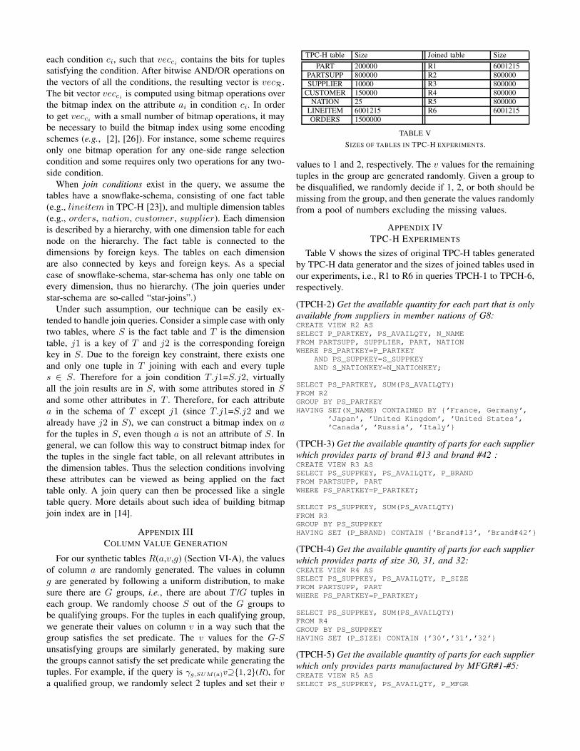
each condition ci, such that vecci contains the bits for tuples

satisfying the condition. After bitwise AND/OR operations on

the vectors of all the conditions, the resulting vector is vecℛ.

The bit vector vecci is computed using bitmap operations over

the bitmap index on the attribute ai in condition ci. In order

to get vecci with a small number of bitmap operations, it may

be necessary to build the bitmap index using some encoding

schemes (e.g., [2], [26]). For instance, some scheme requires

only one bitmap operation for any one-side range selection

condition and some requires only two operations for any two-

side condition.

When join conditions exist in the query, we assume the

tables have a snowflake-schema, consisting of one fact table

(e.g., lineitem in TPC-H [23]), and multiple dimension tables

(e.g., orders, nation, customer, supplier). Each dimension

is described by a hierarchy, with one dimension table for each

node on the hierarchy. The fact table is connected to the

dimensions by foreign keys. The tables on each dimension

are also connected by keys and foreign keys. As a special

case of snowflake-schema, star-schema has only one table on

every dimension, thus no hierarchy. (The join queries under

star-schema are so-called “star-joins”.)

Under such assumption, our technique can be easily ex-

tended to handle join queries. Consider a simple case with only

two tables, where S is the fact table and T is the dimension

table, j1 is a key of T and j2 is the corresponding foreign

key in S. Due to the foreign key constraint, there exists one

and only one tuple in T joining with each and every tuple

s ∈ S. Therefore for a join condition T.j1=S.j2, virtually

all the join results are in S, with some attributes stored in Sand some other attributes in T . Therefore, for each attribute

a in the schema of T except j1 (since T.j1=S.j2 and we

already have j2 in S), we can construct a bitmap index on afor the tuples in S, even though a is not an attribute of S. In

general, we can follow this way to construct bitmap index for

the tuples in the single fact table, on all relevant attributes in

the dimension tables. Thus the selection conditions involving

these attributes can be viewed as being applied on the fact

table only. A join query can then be processed like a single

table query. More details about such idea of building bitmap

join index are in [14].

APPENDIX III

COLUMN VALUE GENERATION

For our synthetic tables R(a,v,g) (Section VI-A), the values

of column a are randomly generated. The values in column

g are generated by following a uniform distribution, to make

sure there are G groups, i.e., there are about T /G tuples in

each group. We randomly choose S out of the G groups to

be qualifying groups. For the tuples in each qualifying group,

we generate their values on column v in a way such that the

group satisfies the set predicate. The v values for the G-Sunsatisfying groups are similarly generated, by making sure

the groups cannot satisfy the set predicate while generating the

tuples. For example, if the query is g,SUM(a)v⊇{1, 2}(R), for

a qualified group, we randomly select 2 tuples and set their v

TPC-H table Size Joined table Size

PART 200000 R1 6001215

PARTSUPP 800000 R2 800000

SUPPLIER 10000 R3 800000

CUSTOMER 150000 R4 800000

NATION 25 R5 800000

LINEITEM 6001215 R6 6001215

ORDERS 1500000

TABLE V

SIZES OF TABLES IN TPC-H EXPERIMENTS.

values to 1 and 2, respectively. The v values for the remaining

tuples in the group are generated randomly. Given a group to

be disqualified, we randomly decide if 1, 2, or both should be

missing from the group, and then generate the values randomly

from a pool of numbers excluding the missing values.

APPENDIX IV

TPC-H EXPERIMENTS

Table V shows the sizes of original TPC-H tables generated

by TPC-H data generator and the sizes of joined tables used in

our experiments, i.e., R1 to R6 in queries TPCH-1 to TPCH-6,

respectively.

(TPCH-2) Get the available quantity for each part that is only

available from suppliers in member nations of G8:CREATE VIEW R2 AS

SELECT P_PARTKEY, PS_AVAILQTY, N_NAME

FROM PARTSUPP, SUPPLIER, PART, NATION

WHERE PS_PARTKEY=P_PARTKEY

AND PS_SUPPKEY=S_SUPPKEY

AND S_NATIONKEY=N_NATIONKEY;

SELECT PS_PARTKEY, SUM(PS_AVAILQTY)

FROM R2

GROUP BY PS_PARTKEY

HAVING SET(N_NAME) CONTAINED BY {’France, Germany’,

’Japan’, ’United Kingdom’, ’United States’,

’Canada’, ’Russia’, ’Italy’}

(TPCH-3) Get the available quantity of parts for each supplier

which provides parts of brand #13 and brand #42 :CREATE VIEW R3 AS

SELECT PS_SUPPKEY, PS_AVAILQTY, P_BRAND

FROM PARTSUPP, PART

WHERE PS_PARTKEY=P_PARTKEY;

SELECT PS_SUPPKEY, SUM(PS_AVAILQTY)

FROM R3

GROUP BY PS_SUPPKEY

HAVING SET (P_BRAND) CONTAIN {’Brand#13’, ’Brand#42’}


which provides parts of size 30, 31, and 32:CREATE VIEW R4 AS

SELECT PS_SUPPKEY, PS_AVAILQTY, P_SIZE

FROM PARTSUPP, PART



FROM R4

GROUP BY PS_SUPPKEY

HAVING SET (P_SIZE) CONTAIN {’30’,’31’,’32’}


which only provides parts manufactured by MFGR#1-#5:CREATE VIEW R5 AS

SELECT PS_SUPPKEY, PS_AVAILQTY, P_MFGR

300

400

500

600

700

800

900

Exe

cuti

on

Tim

e (

mse

cs.)

contain contained by equal

0

100

200

300

400

500

600

700

800

900

1 3 5 7 9 20 40 60 80 100Exe

cuti

on

Tim

e (

mse

cs.)

C


3000

4000

5000

6000

7000

8000

Exe

cuti

on

Tim

e (

mse

cs.)


0

1000

2000

3000

4000

5000

6000

7000

8000

1 10 100 1000Exe

cuti

on

Tim

e (

mse

cs.)

S


2000

3000

4000

5000

6000

7000

8000

Exe

cuti

on

Tim

e (

mse

cs.)


0

1000

2000

3000

4000

5000

6000

7000

8000

10 100 1000 10000 100000

Exe

cuti

on

Tim

e (

mse

cs.)

G


100

1000

10000

Exe

cuti

on

Tim

e (

mse

cs.)


1

10

100

1000

10000

10000 100000 1000000

Exe

cuti

on

Tim

e (

mse

cs.)

T


20%

40%

60%

80%

100%

Bre

ak

do

wn

of

Exe

cu

tio

n T

ime

scan find_group agg

0%

20%

40%

60%

80%

100%

⊇ ⊆ = ⊇ ⊆ = ⊇ ⊆ =

1 10 100

Bre

ak

do

wn

of

Exe

cu

tio

n T

ime

C

scan find_group agg

0%

20%

40%

60%

80%

100%

Bre

ak

do

wn

of

Exe

cu

tio

n T

ime

scan find_group agg

0%

20%

40%

60%

80%

100%

⊇ ⊆ = ⊇ ⊆ = ⊇ ⊆ = ⊇ ⊆ =

1 10 100 1000B

rea

kd

ow

n o

f

Exe

cu

tio

n T

ime

S

scan find_group agg

0%

20%

40%

60%

80%

100%

Bre

ak

do

wn

of

Exe

cu

tio

n T

ime

scan find_group agg

0%

20%

40%

60%

80%

100%

⊇ ⊆ = ⊇ ⊆ = ⊇ ⊆ =

10 1000 100000

Bre

ak

do

wn

of

Exe

cu

tio

n T

ime

G

scan find_group agg

0%

20%

40%

60%

80%

100%

Bre

ak

do

wn

of

Exe

cu

tio

n T

ime

scan find_group agg

0%

20%

40%

60%

80%

100%

⊇ ⊆ = ⊇ ⊆ = ⊇ ⊆ =

10000 100000 1000000

Bre

ak

do

wn

of

Exe

cu

tio

n T

ime

T

scan find_group agg


Fig. 6. Execution time of Rewrt and its breakdown.

40

60

80

100

Exe

cuti

on

Tim

e (

mse

cs.)


0

20

40

60

80

100

1 3 5 7 9 20 40 60 80 100Exe

cuti

on

Tim

e (

mse

cs.)

C


200

300

400

500

600

700

Exe

cuti

on

Tim

e (

mse

cs.)


0

100

200

300

400

500

600

700

1 10 100 1000

Exe

cuti

on

Tim

e (

mse

cs.)

S


400

600

800

1000

1200

Exe

cuti

on

Tim

e (

mse

cs.)


0

200

400

600

800

1000

1200

10 100 1000 10000 100000

Exe

cuti

on

Tim

e (

mse

cs.)

G


10

100

1000

Exe

cuti

on

Tim

e (

mse

cs.)


1

10

100

1000

10000 100000 1000000

Exe

cuti

on

Tim

e (

mse

cs.)

T


0%

20%

40%

60%

80%

100%

Bre

ak

do

wn

of

Exe

cu

tio

n T

ime

scan the rest

0%

20%

40%

60%

80%

100%

⊇ ⊆ =

⊇ ⊆ =

⊇ ⊆ =

1 10 100

Bre

ak

do

wn

of

Exe

cu

tio

n T

ime

C

scan the rest

0%

20%

40%

60%

80%

100%

Bre

ak

do

wn

of

Exe

cu

tio

n T

ime

scan the rest

0%

20%

40%

60%

80%

100%

⊇ ⊆ = ⊇ ⊆ = ⊇ ⊆ = ⊇ ⊆ =

1 10 100 1000

Bre

ak

do

wn

of

Exe

cu

tio

n T

ime

S

scan the rest

0%

20%

40%

60%

80%

100%

Bre

ak

do

wn

of

Exe

cu

tio

n T

ime

scan the rest

0%

20%

40%

60%

80%

100%

⊇ ⊆ = ⊇ ⊆ = ⊇ ⊆ =

1 10 100

Bre

ak

do

wn

of

Exe

cu

tio

n T

ime

G

scan the rest

0%

20%

40%

60%

80%

100%

Bre

ak

do

wn

of

Exe

cu

tio

n T

ime

scan the rest

0%

20%

40%

60%

80%

100%

⊇ ⊆ = ⊇ ⊆ = ⊇ ⊆ =

1 10 100

Bre

ak

do

wn

of

Exe

cu

tio

n T

ime

T

scan the rest


Fig. 7. Execution time of Agg and its breakdown.

FROM PARTSUPP, PART



FROM R5

GROUP BY PS_SUPPKEY

HAVING SET (P_MFGR) CONTAINED BY {’MFGR#1’,’MFGR#2’,

’MFGR#3’,’MFGR#4’,’MFGR#5’}

(TPCH-6) Get the total price of orders for each lineitem that

has orders with exactly 5 different priorities, from low to

urgent:CREATE VIEW R6

SELECT L_LINENUMBER, O_TOTALPRICE, O_ORDERPRIORITY

FROM LINEITEM, ORDERS

WHERE L_ORDERKEY=O_ORDERKEY;

SELECT L_LINENUMBER, SUM(O_TOTALPRICE)

FROM R6

GROUP BY L_LINENUMBER

HAVING SET (O_ORDERPRIORITY) EQUAL {’1-URGENT’,

’2-HIGH’,’3-MEDIUM’,’4-NOT SPECIFIED’,’5-LOW’}

APPENDIX V

BREAKDOWN OF REWRT AND AGG

Similar to Figure 5 for Bitmap, the execution time and its

detailed breakdown for Rewrt and Agg are shown in Figure 6

and 7, respectively, for different configuration groups. For

the Rewrt method, the PostgreSQL plans can be roughly

divided into three major steps: Step 1– scan the table (several

times); Step 2– find qualifying groups that satisfy the query

conditions; Step 3– calculate the required aggregates for each

qualifying group. For Agg, we divide the cost into table scan

and the rest. Similar to what we observed for Figure 5,

no single component in the breakdown of Rewrt and Agg

dominates the query execution cost. The breakdown varies as

the configuration parameters change.

Figure 6(a) shows that the execution time of Rewrt, similar

to that of Bitmap, also increases linearly with C (number of

constant values in set predicate). The breakdown also changes

by C. For example, the Step 3 (calculate aggregates) for

CONTAIN (⊇) gets smaller and smaller percentage. We can

understand this by analyzing the plan for the rewritten query

of g,SUM(a) v ⊇ {1,2,3}(R), shown in Figure 8. It performs

multiple index scans in Step 1 and intersects the scan results

in Step 2. Therefore these two steps become more costly as Cincreases. The last step, calculating aggregates, does the same

amount of work, since the aggregating is independent of C.

Figure 6(a) also shows large performance difference between

different operators when C increases. Given T=100K, G=1K,

and S=10, the number of tuples with R.v being 1, 2, ..., or

3.730 ms

SELECT sum(a)FROM R,( ( SELECT DISTINCT g

FROM R

Intersect

Project &

2.643 ms

FROM R WHERE v = 1 )

INTERSECT( SELECT DISTINCT g FROM R WHERE v = 2 )

INTERSECT( SELECT DISTINCT g FROM R WHERE v = 3 )

) AS TMP

Index Scan

R.v=1

Project &

Sort on g

Append

1.450 ms

) AS TMPWHERE R.g = TMP.gGROUP BY R.g

Intersect

Hash Join

Seq Scan

R

Hash Aggregate

3.730 ms 27.842 ms

50.582 ms

51.100 ms

Intersect

Project &

Intersect

Project &

Sort on g

Append

Index Scan

R.v=3

R

0.988 ms

3.651 ms

3.721 ms

Project &

Sort on g

Append

Index Scan

R.v=21.107 ms

2.567 ms

2.633 ms

Fig. 8. Rewrt Query Plan for CONTAIN, 100K tuples, 1K groups, 10

satisfying groups.

C is small, in order to have only 10 out of 1, 000 groups

satisfying the query condition. Therefore for CONTAIN, the

set intersect operator in Figure 8 involves small cost. However

for CONTAINED BY, the filter operator in Figure 2 produces

much more result tuples, making the set difference (Except)

operator more costly.

Figure 7(a) shows that the execution time of Agg, different

from that of Rewrt and Bitmap, is not affected by C. As the

outline in Algorithm 1 shows, the only cost component related

to C is the checking of a tuple’s v value against the given Cconstants (line 8 and 11), which is much cheaper than other

components.

Figure 7(b) shows that the execution time of Agg increases

with S (number of satisfying groups) under some operators

and decreases under others, and the changes are only slight

in both cases. Figure 6(b) shows that the behavior of Rewrt

is similar to Agg with regard to S in that the execution time

increases under some operators and decreases under others.

The variations are small for some operators and larger for

others. For example, the cost of CONTAINED BY decreases

by S. Use Figure 2 to explain again. When more groups satisfy

the query condition, the output cardinality of operator Filter

becomes smaller, resulting in smaller cost of set difference

(Except) operation.

Figure 6(c) shows that, as G (number of groups) in the data

increases, the execution time of Rewrt increases substantially

for CONTAINED BY and EQUAL, but does not change much

for CONTAIN. Use CONTAINED BY as an example. When

G increases, with the number of satisfying groups unchanged,

the number of tuples matching the constants becomes smaller,

resulting in more result tuples from the Filter operator in

Figure 2, making the set difference (Except) operator more

costly. Figure 7(c) shows that the execution time of Agg

increases slowly with G, for the reason similar to why the

execution time is not affected much by C.

Figure 6(d) and Figure 7(d) show that, naturally, Rewrt and

Agg scale linearly with T (number of tuples in the data table),

similar to Bitmap.

Set Predicates in SQL: Enabling Set-Level Comparisons for ... · Set Predicates in SQL: Enabling...

Documents

Transcript of Set Predicates in SQL: Enabling Set-Level Comparisons for ... · Set Predicates in SQL: Enabling...