SESUG - 2013

1

Paper SD-12

Receiver Operating Characteristic (ROC) Curve: comparing parametric estimation, Monte Carlo simulation and numerical integration

Paulo Macedo, Integrity Management Services LLC

ABSTRACT A receiver operating characteristic (ROC) curve is a plot of predictive model probabilities of true positives (sensitivity) as a function of probabilities of false positives (1 – specificity) for a set of possible cutoff points. Some of the SAS/STAT procedures do not have built-in options for ROC curves and there have been a few suggestions in previous SAS forums to address the issue by using either parametric or non-parametric methods to construct those curves. This study shows how a simple concave function verifies the properties necessary to provide good fits to the ROC curve of diverse predictive models, and has also the advantage of giving an exact solution for the estimation of the area under the ROC in terms of a Beta function – defined by the parameters of the concave function. The study proceeds to discuss the implementation of the approach to a working dataset, and compares the value of the area estimated using the parametric solution to the ones obtained through three numerical methods of integration – Trapezoidal Rule, Simpson’s Rule and Gauss Quadrature, and Monte Carlo simulation. Finally the study proposes that the observed data points can be interpreted as part of an underlying data generating process (DGP) by randomly drawing subsets of the available data points – a sampling approach to the estimation of the Area Under the Curve. The SAS products used in the study are SAS BASE and SAS/STAT, in particular PROC NLIN and PROC SURVEYSELECT.

INTRODUCTION The ROC curve evaluates the accuracy of a predictive model – or a test - in separating populations that have two possible classification outcomes (of the yes/no type) such as: 1) high or low writing test scores among high school students conditional on a set of covariates; 2) having or not a particular disease among patients who underwent a diagnostic test; 3) being or not a future credit card defaulter among credit card applicants – as a function of a set of individual characteristics; 4) being or not a fraudulent provider – as a function of set of provider individual/professional characteristics. If a threshold value c is used to include members of a population in the yes group on the basis of the scoring of a model - or a diagnostic test, then the issue of true and false positive rates emerges. The plotting of true positive rates versus false positive rates across all possible thresholds c defines a ROC curve, which makes explicit the set of existing tradeoffs between those rates. The ROC curve “usually has a concave shape connecting the points (0, 0) and (1, 1), and the higher the area under the curve the better the predictions. The ROC curve is more informative than the classification table (which cross-classifies the binary response with a prediction whether the outcome is yes or no), since it summarizes predictive power for all possible thresholds c” (Agresti 2002).

0.00

0.20

0.40

0.60

0.80

1.000.00 0.20 0.40 0.60 0.80 1.00

ROC concave fn equil Lorenz convex fn

Figure 1 ROC concave function and Lorenz convex function

Empirical ROC curves are often estimated from the available finite set of threshold points c by using the pairs of observed true and false positive rates as

corners to: 1) form trapezoids; 2) compute the ROC area as a sum of the sub-areas corresponding to each of these trapezoids (Trapezoidal Rule). An alternate approach to the empirical estimation is to fit a curve to the data. The binormal model is an example of a method frequently employed to do this: it assumes that the positive and the negative outcomes of predictive models (or diagnostic tests) – respectively yes coded as 1 and no coded as 0 – follow two independent normal distributions defined by their own distinct means and standard deviations, and it estimates the area under the ROC curve as a function of parameters associated with the normal distributions that best fit the data. There is a large literature documenting the use of the binormal model as a means to estimate the ROC area. For example, Mithat Gὄnen (2006) provides an extensive discussion of aspects of fitting data to the binormal model including a comparison of the model results with the ones obtained by using the empirical estimation of the ROC curve.

This paper shows how a simple two-parameter concave function may also be a good frame to fit a

SESUG - 2013

2

smooth curve to the data, having also the advantage of giving an exact solution for the estimation of the area under the ROC in terms of a Beta function – defined by the parameters of the concave function. The paper includes five main Sections. Section 1, Functional Form Specification, presents the main features of the two-parameter concave function that anchors the paper discussion about ROC analysis; Section 2, Estimation of the ROC Curve – A Sampling Approach, proposes taking a number of subsets of the available set of data-points as samples drawn from the same data generating process, fitting them iteratively to the chosen functional form and generating a distribution of estimated ROC area values for statistical analysis; Section 3, Performance of Numerical Integration Methods, compares the results produced by the parametric estimation of the ROC area with the figures obtained by using four methods of numerical integration – Trapezoidal Rule, Simpson’s Rule, Gauss Quadrature and Monte Carlo simulation; Section 4, Empirical Estimation of the ROC Area: Trapezoidal Rule Rules, explores options to compute ROC areas with no preliminary estimation of ROC curves (empirical ROC analysis) and compares the estimated areas obtained by the Trapezoidal Rule and a version of the Gauss Quadrature method that uses interpolated ordinates y rather than the unavailable set of points in the curve; Section 5 concludes the paper.

FUNCTIONAL FORM SPECIFICATION AND WORKING DATASET The feasibility of using functional forms other than the binormal model was illustrated by the contribution by Stober and Yeh (2002) to the NESUG 15. The authors first borrowed a convex curve specification proposed by Rasche et al (1980) to estimate the Lorenz curve and its related Gini coefficient, a measurement of income inequality frequently used by economists. They proceeded then to estimate the area under the ROC curve by using the relationship between the ROC curve and the Gini coefficient, ROC = 0.5(Gini + 1). The relationship is well known in the literature. For example, Flach (2010), puts the association in the context of “a linear rescaling of the Area Under (ROC) Curve or AUC as Gini = 2AUC – 1,” the inverse relationship.

This paper proposes a more direct method than the convex function approach – a simple concave function that verifies all the necessary requirements of a typical ROC Curve and it is defined by just two parameters as in the Lorenz curve case. A functional specification y = f(x) of a ROC Curve should satisfy the following conditions:

a) if x (1 – Specificity) = 0, y (Sensitivity) = 0; b) if x = 1, y = 1; c) y > x; d) the slope of the curve is nonnegative and monotonically increasing (meaning that increasing values of x are associated with strictly increasing values of y).

Following the conditions mentioned above and some additional technical requirements, we suggest that the functional form

where

is a proper framework to represent a ROC Curve. Specifically, the function is defined as

for

meaning that at the points 0 and 1 the function assumes values on the equilibrium line

The other conditions satisfied by the function are:

is infinite for any meaning that at the slope of the function is the vertical axis;

is zero for any meaning that at the slope of the function is parallel to the horizontal axis;

for and , that means, the function is concave; if α and β are simultaneously equal to 1 then the function collapses to the equilibrium line

meaning that the area under the ROC Curve has 0.5 as lower bound (equilibrium line ) and 1 as upper bound.

The statistic to compute the area under the ROC curve for the functional relationship above is

A similar integral was analyzed by Rasche et al (1980) in their paper about estimating the (convex) Lorenz curve and the authors used a transformation of variables to evaluate the result in terms of a Beta function. The corresponding

SESUG - 2013

3

transformation of variables for the concave function above is . The reworked expression

for the ROC area is

dz, where the second term identifies a particular Beta function,

whose value can be evaluated by using the Gamma function by means of the known relationship

between the Beta and the Gamma function Γ,

This paper uses as its working dataset the one made publicly available by the University of California at Los Angeles (UCLA) in its demonstration of the main characteristics of the SAS Proc Logistic, “SAS Annotated Output Proc Logistic” (website link available at the References Section). The advantage of using a SAS procedure that has built-in options for ROC-related information (including the area under the ROC curve) is that it can work as a benchmark for gauging the accuracy of the approaches discussed in this paper. The data of the UCLA example “were collected on 200 high school students, with measurements on various tests, including science, math, reading and social studies. The response variable is high writing test score (honcomp), where a writing score greater than or equal to 60 is considered high, and less than 60 considered low; from which we explore its relationship with gender (female), reading test score (read), and science test score (science).” This UCLA dataset can be downloaded from http://www.ats.ucla.edu/stat/sas/webbooks/reg/default.htm.

The next Section discusses methods to compute the area under a curve estimated by using an available set of pair-wise values of true positive (sensitivity) and false positive (1 – specificity) data points. The first step involves fitting the data to the proposed two-parameter concave function using the SAS non-linear regression PROC NLIN, which generates estimates for the parameters α and β and thus the value of the ROC area by means of the corresponding evaluation of the Beta function. After that the Section proceeds to implement the computation of the ROC using three different methods of numerical integration and a Monte Carlo simulation to evaluate how good the results are as compared to the one based on the Beta function.

ESTIMATION OF THE AREA UNDER THE ROC CURVE – A SAMPLING APPROACH The computation of the area under the ROC curve proposed here involves essentially two steps: 1) use of data points defined by pair-wise values of true and false positive rates to estimate a non-linear regression whose framework is the two-parameter function discussed in the previous Section. The model is fit to the data by means of the SAS PROC NLIN, which uses the least squares method as estimator; 2) computation of the area under the estimated curve by using the Beta function estimated parameters as explained before.

This method computes one value for the area under the curve per set of available data points. Rather than use all the points to obtain a single estimate of the ROC area, if possible it is preferable to: 1) take a number of subsets of the available set of data-points as samples drawn from the same data generating process (DGP); 2) compute diverse values for the area and to construct a confidence interval around the average result. The UCLA exercise illustrating the use of the SAS PROC LOGISTIC includes data on 200 high school students and allows for this possibility. Besides generating an estimate for the area under the ROC curve – which works as a benchmark to assess the accuracy of other methods discussed in this Section, the UCLA use of PROC LOGISTIC provides also an output file including a set of 165 data-points (pair-wise values of true and false positive rates) from which distinct subsets of values can be drawn – all having in common the same underlying DGP. Some other statistical applications of the binary classifier type (yes/no outcome) may not have available these data-points but their determination can get done by the recursive use of the PROC FREQ for diverse values of thresholds.

The code below implements the data processing by drawing as samples subsets of the 165 data points available in the UCLA example in a sequence of steps. First it sorts the data points by their false positive figures (1 – specificity), then it removes the first and last false positive value (endpoints) from the sampling universe and finally it proceeds to draw samples of 40 items from the 163 remaining data points. The sampling process generates different subsets of data points including the 40 sampled items added by the two endpoints – a total of 42 items. The SAS code for the data processing implements five batches of samples whose generation is triggered by feeding distinct initial seeds to the SAS random numbers generator. The simulations use batches of 500, 750, 1,000, 1,500 and 2,000 samples.

The data processing uses PROC NLIN, which applies the Least Squares Method (in a non-linear regression model context) to fit the 42 data points of each sample to the two-parameter concave function framework discussed in the previous Section. Every sample generates then a ROC Area value, so PROC MEANS is handy to produce summary figures per batch - the Mean and Standard Deviation – and to allow for the construction of a confidence interval

SESUG - 2013

4

around the Mean.

Table I below displays the results of simulations done using batches samples of size 42 drawn from the 165 available data-points (pairs of values of proportions of true and false positive rates for different cutoffs). The Table summarizes the analysis of samples per batch by including the mean value of the ROC area estimated across samples plus the estimated parameters and the ROC area for the curve whose area value is closer to the mean value computed for the batch – a curve that can be seen as “representative” of the batch. The mean values of ROC areas computed for different batches are consistent to the third decimal place in spite of the existence of some variability in the parameters estimated for the representative curves of the five batches (coefficient of variation around 5%).

Estimate of "a" for Sample Area Closer to the Mean Value

Estimate of "b" for Sample Area Closer to the Mean Value

Curve-specific (a, b) ROC Area

SeedMean ROC Area Across Samples

Absolute Value Difference

Number of samples

0.269323356 0.733621705 0.860490271 6808 0.860490155 1.15962E-07 2,0000.307160623 0.666643771 0.860474687 7545 0.860487157 1.24703E-05 1,5000.30763935 0.666221422 0.860364883 7964 0.860358524 6.35886E-06 1,000

0.331194317 0.628714205 0.860490421 6704 0.860494279 3.85782E-06 7500.304477536 0.671391109 0.86038225 6923 0.860382874 6.24429E-07 500

Table 1 Estimated Parameters for Curves with Computed Areas Closer to the Mean Value Across Samples

Table 2 displays the 95% confidence intervals constructed for the ROC areas around their mean values - computed for the batches using their respective standard deviations. It is worth mentioning that all batches have confidence intervals including the value of the ROC area produced by PROC LOGISTIC in the UCLA annotated example, 0.857, in spite of this figure being close to the lower bound of the intervals in all cases.

Mean ROC Area Across Samples

StdDev ROC Area Across Samples

Lower Bound 95% Upper Bound 95% Number of samples

0.860490155 0.002806499 0.854989417 0.865990894 2,0000.860487157 0.002675267 0.855243635 0.86573068 1,5000.860358524 0.002719149 0.855028992 0.865688056 1,0000.860494279 0.002806814 0.854992922 0.865995635 7500.860382874 0.002721102 0.855049515 0.865716234 500

Table 2 Confidence Intervals for Five ROC Area Means Estimated Across Samples

Code to generate batches of samples /***************************************************** Macro seeds generates 9,000 four-digit random numbers from which a set of N randomly selected are used as seeds for the sample realizations to be drawn from the population of pair-wise true and false positive values *****************************************************/ %macro seeds(initial_seed, samples); %global n; %let n = &samples; data sequence; do seed = 1000 to 9999; shuffle=RANUNI(&initial_seed); output ; end ; run; Proc Sort data=sequence; by descending shuffle; run; Data sequence(drop = shuffle); set sequence; if _N_ <= &samples; run; %mend seeds; %seeds(5432, 2000);

SESUG - 2013

5

%seeds(7890, 1500) %seeds(1234, 1000); %seeds(6543, 750); %seeds(8765, 500); PROC PRINTTO LOG="\\path\Log.txt"; /***************************************** Macro samples generates batches of samples *****************************************/ Options Symbolgen Mlogic; %macro samples; %global i; %do i = 1 %to &n; Data seed_&i; set sequence; if _N_ = &i; Call symput('seed', seed); run; /********************************** Sample size (minus endpoints) = 40 **********************************/ proc surveyselect noprint data=Dsin method=srs n=40 seed=&seed out=sample_&i; run; Data sample_&i; set sample_&i Endpoints; run; Proc Sort Data = sample_&i; by seq; run; /******************************** Proc NLIN fits data to concave fn using the Least Squares Method ********************************/ proc nlin data= sample_&i noprint maxiter = 100 converge = .1; parms a1 = 0.5 b1 = 0.6; bounds 0 < a1 <= 1, 0 < b1 <= 1; model y = 1 - (1 - x**b1)**(1/a1); output out=output parms = a1 b1; quit; /********************************************************* Data step selects one record of previous output to pass on estimated parameters to the next processing step for the ROC Area computation. Any observation number works. *********************************************************/ Data reg_parms_&i; set Output; if _N_=20; run;

SESUG - 2013

6

/*********************************************** Data step computes the area under the ROC curve ***********************************************/ data reg_parms_&i; set reg_parms_&i; aa1 = 1 / a1 + 1; bb1 = (1/ b1); c1 = aa1 + bb1; roc = 1.0 - (1/ b1) * (gamma(aa1) * gamma(bb1) / gamma(c1)); drop aa1 bb1 c1; run; Data reg_parms_&i; set reg_parms_&i; sample = &i; seed = &seed; run; %if &i = 1 %then %do; Data area_values_&n._obs; set reg_parms_&i; run; %end; %else %do; Data area_values_&n._obs; set area_values_&n._obs reg_parms_&i; run; %end; Proc SQL; drop table reg_parms_&i table sample_&i table seed_&i; run; %end; /* statement ends do loop */ Data area_values_&n._obs; set area_values_&n._obs; drop y x seq; run; %mend samples; %samples; Proc Printto; run; %macro area_randomized; proc means data =area_values_&n._obs noprint; var roc; output out = summary_area_values_&n._obs n = mean = std = range = min = max = median = /autoname; run; Data summary_area_values_&n._obs; set summary_area_values_&n._obs; lower_bound_95 = roc_Mean - 1.96*roc_StdDev; upper_bound_95 = roc_Mean + 1.96*roc_StdDev; run; Data _NULL_; set summary_area_values_&n._obs; call symput('mean', roc_Mean); run;

SESUG - 2013

7

Data area_values_&n._obs; set area_values_&n._obs; mean = &Mean; abs_val_difference = ABS(roc - mean); run; Proc sort data = area_values_&n._obs; by abs_val_difference; run; %mend area_randomized; %area_randomized;

PERFORMANCE OF NUMERICAL INTEGRATION METHODS If a set of data points is large enough to allow for drawing subsets as samples of data to be fit to a pre-defined functional form then the approach is worth taking because it takes into consideration the degree of randomness inherent to the data generating process: computing a batch of ROC area values rather than a single value is a way to make this randomness explicit. Either because the set of data points is not large enough or because of individual preference, an analyst may prefer to consider the whole set of available observations as it is – not a to-be-sampled universe - and proceed to implement an empirical estimation of the ROC curve. The Trapezoidal Rule is often used in this case: the area under the ROC curve is computed as a sum of sub-areas formed by the corners of the observed data points. However, the Trapezoidal Rule is just one of a set of numerical methods available for the computation of areas under curves, which are also called Quadrature methods. It is interesting to check if some other numerical methods are useful to address the issue of estimating the ROC area, so this Section discusses briefly some of these methods and proceeds to illustrate their performance using a sample of ROC data points. The description of the technical aspects of numerical integration draws from Lanczos (1988), Judd (1999), Keesling (undated manuscript) and the Section “Numerical Methods – Areas” from the website Digital Library of Mathematical Functions of the National Institute for Standards and Technology. The empirical part of the analysis uses a subset of the UCLA data to rank the performance of a number of Quadrature methods given the availability of a function describing the curve, which is estimated by the PROC NLIN in the way explained before. The methods considered are the Trapezoidal Rule, the Simpson’s rule, the Gauss Quadrature and a crude Monte Carlo simulation. Their performances are evaluated against the benchmark value of the area obtained through the evaluation of the Beta function at the point defined by the two parameters estimated for the non-linear model concave function. The following Section compares two numerical methods – Trapezoidal Rule and Gauss Quadrature, according to their ability to estimate empirical ROC curves. The benchmark curve against which the methods are evaluated is the most representative of the batch of 2,000 samples - representative in the sense that its ROC area is the closest to the mean value of ROC areas computed across the 2,000 samples. The coefficients estimated for this curve, a = 0.269323515 and b = 0.7336214524, are displayed in the first entry of Table 1 as well as the ROC area whose value is 0.8604902569. The estimation uses PROC NLIN to fit data from a sample of 42 data points drawn from the 165 observations generated by the UCLA PROC LOGISTIC by means of PROC SURVEYSELECT with seed = 6,808. The code below implements the data processing steps.

Code to generate the curve of a specific sample (seed = 6808 in this case) %macro samples(seed); proc surveyselect noprint data=Dsin method=srs n=40 seed=&seed out=sample_seed_&seed; run; Data sample_seed_&seed; set sample_seed_&seed Endpoints; run; Proc Sort Data = sample_seed_&seed; by seq; run; /* Proc NLIN fits data to concave fn */ /* using Least Squares Method */

SESUG - 2013

8

proc nlin data= sample_seed_&seed noprint maxiter = 100 converge = .1; parms a1 = 0.5 b1 = 0.6; bounds 0 < a1 <= 1, 0 < b1 <= 1; model y = 1 - (1 - x**b1)**(1/a1); output out=output parms = a1 b1; quit; Data reg_parms_&seed; set Output; if _N_=20; /* any valid observation number works */ run; /* data step retrieves information on coefficients */ /* and computes the area under the ROC curve */ data reg_parms_&seed; set reg_parms_&seed; aa1 = 1 / a1 + 1; bb1 = (1/ b1); c1 = aa1 + bb1; roc = 1.0 - (1/ b1) * (gamma(aa1) * gamma(bb1) / gamma(c1)); drop aa1 bb1 c1; run; Data reg_parms_&seed; set reg_parms_&seed; seed = &seed; run; Data area_values_obs_&seed; set reg_parms_&seed; run; Proc SQL; drop table reg_parms_&seed /* table sample_seed_&seed */ ; run; Data area_values_obs_&seed; set area_values_obs_&seed; drop y x seq; run; %mend samples; %samples (6808); A ROC curve defines a continuum of threshold observations relating true to false positive data points. If such a curve is available, an elementary Trapezoidal Rule (TR) - defined by the equidistance spacing between its x values (false positives) - is an option for computing the area under the curve. The method requires that observed y values (true positives) be connected by straight lines allowing for the insertion of polygons under the curve so that its area is approximated by the area under the polygon. The TR uses n equally spaced data points to compute the area under a curve A, defined in the interval [a, b] as follows

, where

The implementation of the formula above is straightforward and the SAS code is not reproduced here. The required information includes the lower and upper limit of x values (false positives) – set to the standard values of 0 and 1, the

number of intervals n and the function , defined here by the values of the parameters α and β estimated for a sample obtained from a batch of 2,000 samples (seed = 6,808): 0.269323356 and 0.733621705, respectively. The TR method estimates the ROC area as 0.8596526795 for n = 40 and 0.8603176069 for n = 100.

SESUG - 2013

9

The latter number is closer to 0.8604902569, which is the value generated by the benchmark closed form computation The Simpson’s Rule (SR) method of approximating curves and evaluating areas under them uses parabolas of second degree to connect the available discrete data points. The parabolas are of the form y = a + bx + cx2 and each of them requires connecting three ordinates y (true positives), instead of connecting two by straight lines as in the case of the Trapezoidal Rule. Because each parabola spans two intervals, the method can only be used in a straightforward way if the number of intervals is even (and accordingly the number of ordinates odd). The constraint can be relaxed by using a different construction for the last three (or the first three) intervals but this option will not be considered here.

The SR method computes the area under a curve A by separating even and odd ordinates y and associating them with different weights. The formula below computes the area A for an odd number of observations n (even number of intervals n – 1):

, where

The implementation of the formula is also straightforward but it requires the additional step of identifying even and odd ordinates y, which can be done by using an if-then-else clause including the SAS function MOD. The SAS code is not reproduced here. The required information to compute the area includes the lower and upper limit of x values (false positives) – set to the standard values of 0 and 1, the number of intervals n and the function

, defined in this case by the values of the parameters α and β estimated for a sample obtained from a batch of 2,000 samples (seed = 6,808): 0.269323356 and 0.733621705, respectively. The SR method estimates the ROC area 0.860290201 for n = 40 and 0.8604502282 for n = 100. As expected, both the Trapezoidal Rule and the Simpson’s Rule approach the benchmark closed form computation, 0.8604902569 (as the number of data points n increases), but the SR method always performs slightly better: the TR values are 0.8596526795 and 0.8603176069, respectively. Numerical methods like the Trapezoid and the Simpson’s Rules (TR and SR) are derived by integrating interpolating polynomials – first degree (straight line) and second degree (parabola) respectively. The formulas for TR is exact when approximating the value of the area under a function (curve) of degree equal to 1, precisely a + bx; in a similar way, the formula for SR is exact when approximating the value of the area under any function (curve) of degree less or equal to 2, a + bx or y = a + x + bx2. In general the functions to be evaluated are more complex that that so both methods actually compute approximated values for the areas. The TR and the SR methods have x points (false positives) located in positions known apriori because they are evenly spaced between 0 and 1.The main idea behind the Gauss Quadrature is to allow the location of the x points to vary so that it can further increase the degree of the polynomial whose area can be computed exactly for a given number of integration points. The interpolatory Gauss-Legendre Quadrature Rule approximates the area under the curve y = f(x) in the interval [a, b] as

Tables with values for x (often called nodes) and the weights w for different degrees of polynomial functions are widely available – for example, the website of the Digital Library of Mathematical Functions http://dlmf.nist.gov/3.5#v.

A look at the site’s “Table 3.5.2: Nodes and weights for the 10-point Gauss–Legendre formula” puts in perspective the advantages of the method. This table gives the location of points x and the values of weights w for implementing the method based on a polynomial function of degree n = 9. The Gauss–Legendre formula gives an exact solution to the computation of any polynomial function of degree 2n + 1, which in the case of the 10-point formula is 19. Polynomial functions having degrees greater than 19 still get better approximation values in computing areas than the TR and SR methods if similar number of x points are used.

It is worth noting that the tables including the Gauss-Legendre nodes and weights have their displayed values computed for limits of integration set to the interval [-1, 1] so its utilization in the context of ROC analysis requires mapping of these values to the admissible range of x (false positives) numbers, that means the interval [0, 1]. In this case the necessary transformation of variables is accomplished by

x = 0.5 + 0.5x0

SESUG - 2013

10

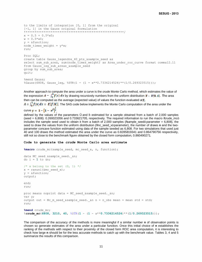
w = 0.5w0 The following SAS code implements the 40-point Gauss-Legendre formula using the function , defined as before by the values of the parameters α and β estimated for a sample obtained from a batch of 2,000 samples (seed = 6,808): 0.269323356 and 0.733621705, respectively. The Gauss-Legendre method evaluates the area as 0.86049090827, a value very close to the benchmark figure obtained by the closed form computation, 0.8604902569.

Code to generate the Gauss-Legendre area estimation /************************************************************ Nodes and weights for the 40-point Gauss–Legendre formula are obtainable from the website "Digital Library of Mathematical Functions," available at http://dlmf.nist.gov/3.5#v ************************************************************/ Data Gauss_leg_plus; INPUT x0 w0; Format x0 22.21 w0 22.21; Datalines; 0.038772417506050821933 0.077505947978424811264 0.116084070675255208483 0.077039818164247965588 0.192697580701371099716 0.076110361900626242372 0.268152185007253681141 0.074723169057968264200 0.341994090825758473007 0.072886582395804059061 0.413779204371605001525 0.070611647391286779696 0.483075801686178712909 0.067912045815233903826 0.549467125095128202076 0.064804013456601038075 0.612553889667980237953 0.061306242492928939167 0.671956684614179548379 0.057439769099391551367 0.727318255189927103281 0.053227846983936824355 0.778305651426519387695 0.048695807635072232061 0.824612230833311663196 0.043870908185673271992 0.865959503212259503821 0.038782167974472017640 0.902098806968874296728 0.033460195282547847393 0.932812808278676533361 0.027937006980023401099 0.957916819213791655805 0.022245849194166957262 0.977259949983774262663 0.016421058381907888713 0.990726238699457006453 0.010498284531152813615 0.998237709710559200350 0.004521277098533191258 ; /**************************************** the nodes x0 < 0 have the same weights w0 as their positive counterparts ****************************************/ Data Gauss_leg_minus; set Gauss_leg_plus; x0 = -x0; run; Data Gauss_leg; set Gauss_leg_plus Gauss_leg_minus; run; Proc Sort data = Gauss_leg; by x0; run; %macro Gauss(sample_seed, input, function); Data Gauss_leg_sub_areas_&sample_seed; set &input; sum_sub_area = 1; /******************************************************** the variable transformation adjusts nodes x and weights w

SESUG - 2013

11

to the limits of integration [0, 1] from the original [-1, 1] in the Gauss original formulation ********************************************************/ x = 0.5 + 0.5*x0; w = 0.5*w0; y = &function; node_times_weight = y*w; run; Proc SQL; create table Gauss_legendre_40_pts_&sample_seed as select sum_sub_area, sum(node_times_weight) as Area_under_roc_curve format comma12.11 from Gauss_leg_sub_areas_&sample_seed group by sum_sub_area; quit; %mend Gauss; %Gauss(6808, Gauss_leg, %STR(1 - (1 - x**0.7336214524)**(1/0.269323515)));

Another approach to compute the area under a curve is the crude Monte Carlo method, which estimates the value of the expression by drawing recursively numbers from the uniform distribution . The area then can be computed as the average (expected value) of values the function evaluated at ,

. The SAS code below implements the Monte Carlo computation of the area under the

curve , defined by the values of the parameters α and β estimated for a sample obtained from a batch of 2,000 samples (seed = 6,808): 0.269323356 and 0.733621705, respectively. The required information to run the macro “crude_mc” includes the sample seed used to obtain it from a batch of 2,000 samples (“sample_seed” parameter = 6,808), the seed to draw the values from the uniform distribution (“mc_seed_x” parameter), the number of draws n and the two-parameter concave function estimated using data of the sample seeded as 6,808. For two simulations that used just 40 and 100 draws the method estimated the area under the curve as 0.8285819341 and 0.864790756 respectively, still not so close to the benchmark figure obtained by the closed form computation, 0.860490271. Code to generate the crude Monte Carlo area estimate %macro crude_mc(sample_seed, mc_seed_x, n, function); data MC_seed_&sample_seed._&n; do i = 1 to &n; /* x belong to the set (0, 1) */ x = ranuni(&mc_seed_x); y = &function; output; end; run; proc means noprint data = MC_seed_&sample_seed._&n; var y; output out = Mc_m_seed_&sample_seed._&n n = n_obs mean = mean std = std; run; %mend crude_mc; %crude_mc(6808, 3210, 40, %STR(1 - (1 - x**0.7336214524)**(1/0.269323515)));

The comparison of the accuracy of the methods is more meaningful if a similar number n of observation points is chosen so generate estimates of the area under a particular function. Once this initial choice of n establishes the ranking of the methods with respect to their proximity of the closed form ROC area computation, it is interesting to check how large n should be for the less accurate methods to catch up with the benchmark value. Tables 3, 4 and 5 summarize the results of this comparison.

SESUG - 2013

12

EMPIRICAL ESTIMATION OF THE ROC AREA: TRAPEZOIDAL RULE RULES This Section considers options to compute ROC areas with no preliminary estimation of ROC curves (empirical ROC analysis) and compares the estimated areas obtained by the Trapezoidal Rule with a version of the Gauss Quadrature method that uses interpolated ordinates y rather than the unavailable set of points in the curve.

The Trapezoidal Rule (TR) is the standard choice when a set of pair-wise data points relating true positives (ordinates y) to false positives (abscissas x) are available but the analyst prefers not to estimate the hypothetical ROC curve underlying the data generation process to compute its area. In general the x values will be unevenly spaced in the horizontal axis and the predictive power of a binary classifier for which there are n available data points can be estimated by summing sub-areas defined by the corner points computed using the TR as follows:

There is no straightforward way to deal with the issue of unequal spacing of x values using the Simpson’s Rule so this Section considers instead testing a version of the Gauss Quadrature framework that uses interpolated values for the ordinates y at each of the x points predetermined by the 40-point Gauss–Legendre formula.

The interpolation process works as follows: each of the points x_gl, predetermined by the 40-point Gauss–Legendre formula, has an antecedent x (x_ant) and a subsequent x among the unevenly spaced data points to be analyzed. The value of any y_gl corresponding to a x_gl is computed by adding to the value of an antecedent y_ant the product of the shift between x_gl with respect to its antecedent x_ant and the slope of the line connecting the points (x_ant, y_ant) and (x, y).

This adaptation of the Gauss-Legendre framework is actually a proxy implementation of the method and the interpretation of its outcome is subject to the proviso of how close the interpolated values of the ordinates y may be of the true y of a hypothetical but unavailable curve. A dramatic difference in the results generated by both methods might justify further analysis but they are actually pretty close: the numbers computed using the Trapezoidal Rule and the adapted Gauss-Lagrange method are 0.8545116160 and 0.8535032856 respectively, both close enough to the value of 0.860490271 set by the closed form computation. Although these results diverge just at the third decimal place, the Trapezoidal Rule approach still ranks closer to the benchmark value than the Gauss-Legendre method. The Trapezoidal Rule is also easy to implement and to interpret – qualities that the alternate method does not match. The SAS codes for implementing both methods are provided after the Conclusion Section below.

SESUG - 2013

13

CONCLUSION The two main contributions of this paper are the proposal of a two-parameter concave function as a framework to fit a ROC curve to true and false positive data points, and the suggestion that such points can be interpreted as sampled from an underlying data generating process (DGP). This particular functional form has the advantage of giving an exact solution for the estimation of the area under the ROC in terms of a Beta function – defined by the parameters of the concave function. The sampling approach has the advantage of making explicit the inherent randomness associated with predictive modeling in the form of sampling variation. The “exact solution” provided by the concave function framework is sample-specific and by considering batches of samples the randomness of the DGP is back in place.

The sampling process generates a statistically reliable benchmark value for the ROC area associated with the working dataset and identifies a reference ROC curve, which allows for the testing and ranking of a number of numerical integration methods in terms of their ability to come close to the benchmark result. Given a similar number of data points, the ranking follows a known pattern in terms of accuracy: closer to the benchmark value are the Gauss-Legendre method, Simpson’s Rule, Trapezoidal Rule and Monte Carlo Integration. As expected, the last three methods, which are dependent on the number of data points, converge to the benchmark value when that number increases.

The paper also explores options to compute ROC areas with no preliminary estimation of ROC curves (empirical ROC analysis) and compares the estimated areas obtained by the Trapezoidal Rule and a version of the Gauss Quadrature method that uses interpolated ordinates y (true positives) rather than the unavailable set of points in the curve. The comparison shows that the results diverge just at the third decimal place but the Trapezoidal Rule approach still ranks closer to the benchmark value than the Gauss-Legendre method. The Trapezoidal Rule has also the advantage of simplicity in implementation and interpretation, so it remains the best choice for empirical ROC analysis.

Code for trapezoidal rule with not-equally-spaced intervals between values of x /*************************************** macro requires entering the value of the seed number of the sample, 6808 here ***************************************/ %macro trap_unequal_spacing(seed); Proc sort data = ample_seed_&seed; by x; run; data Sample_seed_&seed._lag; set Sample_seed_&seed; lag_y = lag(y); lag_x = lag(x); sub_area = 0.5*(y + lag_y)*(x - lag_x); sum_sub_area = 1; if lag_x NE .; run; Proc SQL; create table trap_area_uneven_spc_&seed as select sum_sub_area, sum(sub_area) as area format comma11.10 from Sample_seed_&seed._lag group by sum_sub_area; quit; %mend trap_unequal_spacing; %trap_unequal_spacing(6808); Code for the Gauss-Legendre method with interpolated y /******************************************************* import the values of the 40-point Gauss–Legendre formula as file "Gauss_leg_minus" using the read Datelines code on page XX. Note that the negative nodes (x0 < 0) have

SESUG - 2013

14

the same weights w0 as their positive counterparts *******************************************************/ Data Gauss_leg_minus; set Gauss_leg_plus; x0 = -x0; run; Data Gauss_leg; set Gauss_leg_plus Gauss_leg_minus; run; Proc Sort data = Gauss_leg; by x0; run; Data Gauss_leg_v2; set Gauss_leg; sum_sub_area = 1; x = 0.5 + 0.5*x0; w = 0.5*w0; x_gl = lag(x); w_gl = lag(w); run; options symbolgen mlogic; %macro discrete_points(seed); /************************************************** query collapses duplicate values of "x" into single values associated with the highest value of "y"; working file has data from sample whose seed=6808 **************************************************/ Proc SQL; create table Sample_seed_&seed._v2 as select Max(y) as y, Avg(x) as x from Sample_seed_&seed group by x; quit; /* data step adds lagged variables (x and y) */ Data Sample_seed_&seed._v2; set Sample_seed_&seed._v2; lag_x = lag(x); lag_y = lag(y); run; %do i = 1 %to 40; Data _NULL_; set Gauss_leg_v2; if _N_ = &i; call symput('x_gl', x_gl); call symput('w_gl', w_gl); run; Data row_&i; set Sample_seed_&seed._v2; if &x_gl > lag_x and &x_gl <= x then do; x_gl = &x_gl; w_gl = &w_gl; end; else do; x_gl = .; w_gl = .; end; run; data row_&i;

SESUG - 2013

15

set row_&i; if x_gl NE .; run; %end; /* ends first do loop */ %do i = 1 %to 40; %if &i = 1 %then %do; data Sample_seed_&seed._v3; set row_&i; run; %end; %else %do; data Sample_seed_&seed._v3; set Sample_seed_&seed._v3 row_&i; run; %end; Proc SQL; drop table row_&i; quit; %end; /* ends second do loop */ Data Sample_seed_&seed._v3; set Sample_seed_&seed._v3; if x_gl NE .; run; /************************************************************** data step interpolates the value of ordinate y: the value of an ordinate y_gl is equal to the lagged value of y plus the shift between x_gl w.r.t. the (closest)lagged value of x multiplied by the slope of the line bt (lag_x, lag_y) and (x,y) **************************************************************/ Data Sample_seed_&seed._v4; set Sample_seed_&seed._v3; y_gl = lag_y + (x_gl - lag_x)*(y - lag_y)/(x - lag_x); sum_sub_area = 1; run; Proc SQL; create table gauss_legendre_area_&seed as select sum_sub_area, sum(y_gl*w_gl) as area format comma11.10 from Sample_seed_&seed._v4 group by sum_sub_area; quit; Proc SQL; drop table Sample_seed_&seed._v3 table Sample_seed_&seed._v4; quit; %mend discrete_points; %discrete_points(6808);

REFERENCES Agresti, A. (2002). Categorical Data Analysis. Hoboken, NJ: John Wiley & Sons

Flach, P. “ROC Analysis,” Entry to the Encyclopedia of Machine Learning (2010), edited by C. Sammut and G. Webb, Springer. Available at http://www.google.com/url?sa=t&rct=j&q=gini%20coefficient%20and%20the%20auc&source=web&cd=4&cad=rja&ved=0CEYQFjAD&url=http%3A%2F%2Fwww.cs.bris.ac.uk%2F~flach%2Fpapers%2FROCanalysis.pdf&ei=sML7UZz2HvDb4APiuIDgCQ&usg=AFQjCNE4Ka1nKJe_28ZRy10kYcZgiRdjxQ

SESUG - 2013

16

Gὄnen, M. (2006). “Receiver Operating Characteristic (ROC) Curves.” Proceedings of the SAS Users Group International 31. San Francisco, CA. Available at http://www2.sas.com/proceedings/sugi31/210-31.pdf

Judd, K. (1999). Numerical Methods in Economics. Cambridge, MA: The MIT Press

Keesling, J. Gaussian Quadrature. Mathematics Department, University of Florida. Available at http://www.math.ufl.edu/~kees/GaussianQuadrature.pdf

Lanczos, C. (1988). Applied Analysis. Dover Edition reprint of text originally published in 1956 by Prentice-Hall, Englewood Cliffs NJ

National Institute for Standards and Technology, Digital Library of Mathematical Functions. “Numerical Methods – Areas.” Available at http://dlmf.nist.gov/3.5#v

Rasche, R. H., J. Gaffney, A.Y. C. Koo, and N. Obst. (1980). “Functional Forms for Estimating the Lorenz Curve,” Econometrica, 48, pp. 1061-1062, Journal of the Econometric Society

Stober, P. and S.T. Yeh. (2002). “An Explicit Functional Form Specification Approach to Estimate the Area under a Receiver Operating Characteristic (ROC) Curve”. Proceedings of the NESUG 15. Buffalo, NY. Available at http://www.nesug.org/Proceedings/nesug02/ps/ps012.pdf

UCLA Institute for Digital Research and Education website. “SAS Annotated Output Proc Logistic.” Available at http://www.google.com/url?sa=t&rct=j&q=ucla%20logistic%20regression%20sas%20annotated%20output&source=web&cd=1&cad=rja&ved=0CCoQFjAA&url=http%3A%2F%2Fwww.ats.ucla.edu%2Fstat%2Fsas%2Foutput%2Fsas_logit_output.htm&ei=A6v-UaicDcW34APpqIGICA&usg=AFQjCNHuA6gzVOjBySRMMVebFQUnC_3c9g9

CONTACT INFORMATION Your comments and questions are valued and encouraged. Contact the author at:

Name: Paulo Macedo Enterprise: Integrity Management Services Address: 5911 Kingstowne Village Parkway City, State ZIP: 22315 Work Phone: (703) 683-9600 Ext. 408 E-mail: pmacedo@integritym.com

SAS and all other SAS Institute Inc. product or service names are registered trademarks or trademarks of SAS Institute Inc. in the USA and other countries. ® indicates USA registration.

Other brand and product names are trademarks of their respective companies.