Session-Key Generation using Human Passwords Only∗

Oded Goldreich†

Department of Computer ScienceWeizmann Institute of Science

Rehovot, Israel.oded@wisdom.weizmann.ac.il

Yehuda Lindell‡

Department of Computer ScienceBar-Ilan University

Ramat Gan, Israel.lindell@cs.biu.ac.il

January 25, 2005

Abstract

We present session-key generation protocols in a model where the legitimate parties shareonly a human-memorizable password, and there is no additional setup assumption in the net-work. Our protocol is proven secure under the assumption that enhanced trapdoor permutationsexist. The security guarantee holds with respect to probabilistic polynomial-time adversariesthat control the communication channel (between the parties), and may omit, insert and modifymessages at their choice. Loosely speaking, the effect of such an adversary that attacks an exe-cution of our protocol is comparable to an attack in which an adversary is only allowed to makea constant number of queries of the form “is w the password of Party A”. We stress that theresult holds also in case the passwords are selected at random from a small dictionary so thatit is feasible (for the adversary) to scan the entire directory. We note that prior to our result, itwas not known whether or not such protocols were attainable without the use of random oraclesor additional setup assumptions.

Keywords: Session-key generation (authenticated key-exchange), mutual authentication proto-cols, human-memorizable passwords, secure two-party computation, non-malleable commitments,zero-knowledge proofs, pseudorandom generators and functions, message authentication schemes.

∗An extended abstract of this work appeared in Crypto 2001.†Supported by MINERVA Foundation, Germany.‡This work was carried out while the author was at the Weizmann Institute of Science.

Contents

1 Introduction 31.1 What Security May be Achieved Based on Passwords . . . . . . . . . . . . . . . . . . 41.2 Comparison to Other Work . . . . . . . . . . . . . . . . . . . . . . . . . . . . . . . . 51.3 Techniques . . . . . . . . . . . . . . . . . . . . . . . . . . . . . . . . . . . . . . . . . 81.4 Discussion . . . . . . . . . . . . . . . . . . . . . . . . . . . . . . . . . . . . . . . . . . 91.5 Organization . . . . . . . . . . . . . . . . . . . . . . . . . . . . . . . . . . . . . . . . 9

2 Formal Setting 102.1 Basic Notations . . . . . . . . . . . . . . . . . . . . . . . . . . . . . . . . . . . . . . . 102.2 (1− ε)-Indistinguishability and Pseudorandomness . . . . . . . . . . . . . . . . . . . 102.3 Authenticated Session-Key Generation: Definition and Discussion . . . . . . . . . . . 11

2.3.1 Motivation for the definition . . . . . . . . . . . . . . . . . . . . . . . . . . . 122.3.2 The actual definition . . . . . . . . . . . . . . . . . . . . . . . . . . . . . . . . 132.3.3 Properties of Definition 2.4 . . . . . . . . . . . . . . . . . . . . . . . . . . . . 152.3.4 Augmenting the definition . . . . . . . . . . . . . . . . . . . . . . . . . . . . . 162.3.5 Session-key generation as secure multiparty computation . . . . . . . . . . . . 20

2.4 Our Main Result . . . . . . . . . . . . . . . . . . . . . . . . . . . . . . . . . . . . . . 202.5 Multi-Session Security . . . . . . . . . . . . . . . . . . . . . . . . . . . . . . . . . . . 20

2.5.1 Sequential executions for one pair of parties . . . . . . . . . . . . . . . . . . . 202.5.2 Concurrent executions for many pairs of parties . . . . . . . . . . . . . . . . . 24

3 Our Session-Key Generation Protocol 283.1 The Protocol . . . . . . . . . . . . . . . . . . . . . . . . . . . . . . . . . . . . . . . . 283.2 Motivation for the Protocol . . . . . . . . . . . . . . . . . . . . . . . . . . . . . . . . 30

3.2.1 On the general structure of the protocol . . . . . . . . . . . . . . . . . . . . . 303.2.2 On some specific choices . . . . . . . . . . . . . . . . . . . . . . . . . . . . . . 32

3.3 Properties of Protocol 3.2 . . . . . . . . . . . . . . . . . . . . . . . . . . . . . . . . . 33

4 Analysis of Protocol 3.2: Proof Sketches 344.1 Preliminaries . . . . . . . . . . . . . . . . . . . . . . . . . . . . . . . . . . . . . . . . 344.2 Organization and an Outline of the Proof . . . . . . . . . . . . . . . . . . . . . . . . 354.3 The Security of Protocol 3.2 for Passive Adversaries . . . . . . . . . . . . . . . . . . 374.4 The Key-Match Property . . . . . . . . . . . . . . . . . . . . . . . . . . . . . . . . . 39

4.4.1 Case (1) – The unsynchronized case . . . . . . . . . . . . . . . . . . . . . . . 404.4.2 Case (2) – The synchronized case . . . . . . . . . . . . . . . . . . . . . . . . . 42

4.5 Simulating the Stand-Alone (A,C) Execution . . . . . . . . . . . . . . . . . . . . . . 434.6 Simulating the (C,B) Execution . . . . . . . . . . . . . . . . . . . . . . . . . . . . . 45

4.6.1 Step 1: Simulating the (C,B 6dec) execution . . . . . . . . . . . . . . . . . . . . 454.6.2 Step 2: Simulating B’s decision bit . . . . . . . . . . . . . . . . . . . . . . . . 46

4.7 The Security of Protocol 3.2 for Arbitrary Adversaries . . . . . . . . . . . . . . . . . 49

5 Full Proof of Security for Passive Adversaries 51

1

6 Full Proof of the Key-Match Property 546.1 Proof of Lemma 4.6 (The Unsynchronized Case) . . . . . . . . . . . . . . . . . . . 54

6.1.1 Simulating A’s zero-knowledge proof . . . . . . . . . . . . . . . . . . . . . . . 556.1.2 Proof of a modified lemma 4.6 (when C interacts with A6zk and B′) . . . . . . 62

6.2 Proof of Lemma 4.7 (The Synchronized Case) . . . . . . . . . . . . . . . . . . . . . 68

7 Simulating the Stand-Alone (A,C) Execution 71

8 Simulating the (C, B) Execution 758.1 Simulating the (C,B 6dec) Execution . . . . . . . . . . . . . . . . . . . . . . . . . . . . 768.2 Simulating B’s Accept/Reject Decision Bit . . . . . . . . . . . . . . . . . . . . . . . . 778.3 Conclusion . . . . . . . . . . . . . . . . . . . . . . . . . . . . . . . . . . . . . . . . . 80

References 80

A Cryptographic Tools 84A.1 Secure Two-Party Computation . . . . . . . . . . . . . . . . . . . . . . . . . . . . . . 84A.2 String Commitment . . . . . . . . . . . . . . . . . . . . . . . . . . . . . . . . . . . . 87A.3 Non-Malleable String Commitment . . . . . . . . . . . . . . . . . . . . . . . . . . . . 88A.4 The Zero-Knowledge Proof of Richardson and Kilian . . . . . . . . . . . . . . . . . . 89A.5 Seed-Committed Pseudorandom Generators . . . . . . . . . . . . . . . . . . . . . . . 91A.6 Message Authentication Codes (MACs) . . . . . . . . . . . . . . . . . . . . . . . . . 91

2

1 Introduction

This work deals with the oldest and probably most important problem of cryptography: en-abling private and reliable communication among parties that use a public communication channel.Loosely speaking, privacy means that nobody besides the legitimate communicators may learn thedata communicated, and reliability (or integrity) means that nobody may modify the contents ofthe data communicated (without the receiver detecting this fact). Needless to say, a vast amountof research has been invested in this problem. Our contribution refers to a difficult and yet naturalsetting of two parameters of the problem: the adversaries and the initial set-up.

We consider only probabilistic polynomial-time adversaries. Still, even within this framework,an important distinction refers to the type of adversaries one wishes to protect against: passiveadversaries only eavesdrop the channel, whereas active adversaries may also omit, insert and mod-ify messages sent over the channel. Clearly, reliability is a problem only with respect to activeadversaries (and holds by definition w.r.t passive adversaries). We focus on active adversaries.

The second parameter mentioned above is the initial set-up assumptions. Some assumption ofthis form must exist or else there is no difference between the legitimate communicators, called Aliceand Bob, and the adversary (which may otherwise initiate a conversation with Alice pretending tobe Bob). We list some popular initial set-up assumptions and briefly discuss what is known aboutthem.Public-key infrastructure: Here one assumes that each party has generated a secret-key and

deposited a corresponding public-key with some trusted server(s). The latter server(s) may beaccessed at any time by any user.It is easy to establish private and reliable communication in this model (by a straightforward useof the public-key schemes, cf. [21, 52]). (However, even in this case, one may want to establish“session-keys” as discussed below; for example, see [49, 7, 3, 53, 18]).)

Shared (high-quality) secret keys: By high-quality keys we mean strings coming from distri-butions of high entropy (e.g., uniformly chosen 128-bit long strings, uniformly chosen 1024-bitprimes, etc). Furthermore, these keys are selected by a suitable program, and cannot be mem-orized by humans.In case a pair of parties shares such a key, they can conduct private and reliable communication(either directly (cf. [13, 56, 29]) or by first establishing a session-key (cf. [6, 7])).

Shared (low-quality) secret passwords: In contrast to high-quality keys, passwords are stringsthat may be easily selected, memorized and typed-in by humans. An illustrating (and simplified)example is the case in which the password is selected uniformly from a relatively small dictionary;that is, the password is uniformly distributed in D ⊂ {0, 1}n, where |D| = poly(n).Note that using such a password in the role of a cryptographic key (in schemes as mentionedabove) will yield a totally insecure scheme. A more significant observation is that the adversarymay try to guess the password, and initiate a conversation with Alice pretending to be Boband using the guessed password. So nothing can prevent the adversary from successfully im-personating Bob with probability 1/|D|. But can we limit the adversary’s success to about thismuch?

The latter question is the focus of this paper.

Session-keys: The problem of establishing private and reliable communication is commonly re-duced to the problem of generating a secure session-key (a.k.a “authenticated key exchange”).

3

Loosely speaking, one seeks a protocol by which Alice and Bob may agree on a key (to be usedthroughout the rest of the current communication session) so that this key will remain unknownto the adversary.1 Of course, the adversary may prevent such agreement (by simply blocking allcommunication), but this will be detected by either Alice or Bob.

1.1 What Security May be Achieved Based on Passwords

Let us consider the related (although seemingly easier) task of mutual authentication. Here Aliceand Bob merely want to establish that they are talking to one another. Repeating an observationmade above, we note that if the adversary initiates t ≤ |D| instances of the mutual authenticationprotocol, guessing a different password in each of them, then with probability t/|D| it will succeedin impersonating Alice to Bob (and furthermore find the password). The question posed above isrephrased here as follows:

Can one construct a password-based scheme in which the success probability of anyprobabilistic polynomial-time impersonation attack is bounded by O(t/|D|)+µ(n), wheret is the number of sessions initiated by the adversary, and µ(n) is a negligible functionin the security parameter n?

We resolve the above question in the affirmative. That is, assuming the existence of trapdoorone-way permutations, we prove that schemes as above do exist (for any D and specifically for|D| = poly(n)). Our proof is constructive. We actually provide a protocol of comparable securityfor the more demanding goal of authenticated session-key generation.

Password-based authenticated session-key generation: Our definition for the task of au-thenticated session-key generation is based on the simulation paradigm. That is, we require that asecure protocol emulates an ideal execution of a session-key generation protocol (cf. [2, 45, 16]). Insuch an ideal execution, a trusted party hands identical, uniformly distributed session-keys to thehonest parties. The only power given to the adversary in this ideal model is to prevent the trustedparty from handing keys to one of the parties. (We stress that, in this ideal model, the adversarylearns nothing of the parties’ joint password or output session-key).

Next, we consider a real execution of a protocol (where there is no trusted party and the ad-versary has full control over the communication channel between the honest parties). In general, aprotocol is said to be secure if real-model adversaries can be emulated in the ideal-model such thatthe output distributions are computationally indistinguishable. Since in a password-only settingthe adversary can always succeed with probability 1/|D|, it is impossible to achieve computationalindistinguishability between the real model and above-described ideal model (where the adversaryhas zero probability of success). Therefore, in the context of a password-only setting, an authen-ticated session-key generation protocol is said to be secure if the above-mentioned ideal-modelemulation results in an output distribution that can be distinguished from a real execution by (agap of) at most O(1/|D|) + µ(n). (We note that in previous definitions, the probability of adver-sarial success was made strictly 1/|D| rather than O(1/|D|); we do not know how to achieve thisstricter requirement.)

1We stress that many famous key-exchange protocols, such as the one of Diffie and Hellman [21], refer to a passiveadversary. In contrast, this paper refers to active adversaries.

4

Main result (informally stated): Assuming the existence of 1–1 one-way functions and collec-tions of enhanced trapdoor one-way permutations,2 there exists a secure authenticated session-keygeneration protocol in the password-only setting.

We stress that the above (informal) definition implies the intuitive properties of authenticatedsession-key generation (e.g., security of the generated session-key and of the initial password). Inparticular, the output session-key can be distinguished from a random key by (a gap of) at mostO(1/|D|) + µ(n). This implies that when using the session-key as a key to a MAC, for example,the probability that any polynomial-time adversary can generate a valid MAC-tag to a messagenot sent by the legitimate party is small (i.e., O(1/|D|) + µ(n)). We stress that the session-keycan be used for polynomially-many MACs and the probability that the adversary will forge evenone message still remains bounded by O(1/|D|) + µ(n). Likewise, when using the session key forprivate-key encryption, the probability that the adversary learns anything about the encryptedmessages is small. That is, for every partial-information function, the adversary can guess thevalue of the function applied to the messages with O(1/|D|) + µ(n) advantage over the a-prioriprobability. This success probability is exactly the same (ignoring µ(n) and constant factors) as forthe naive adversary who just attempts to guess the password and succeeds with probability 1/|D|.See Section 2.3.3 for more discussion.

In addition to the above-described security of the session-key, the definition guarantees that thedistinguishing gap between the parties’ joint password and a uniformly distributed element in D isat most O(1/|D|) + µ(n). (As we have mentioned, the fact that the adversary can distinguish withgap O(1/|D|) is an inherent limitation of password-based security.) The parties are also guaranteedthat, except with probability O(1/|D|)+µ(n), they either end-up with the same session-key or detectthat their communication has been tampered with. Our definition also implies additional desirableproperties of session-key protocols such as forward secrecy and security in the case of session-keyloss (or known-key attacks). Furthermore, our protocol provides improved (i.e., negligible gap)security in case the adversary only eavesdrops the communication (during the protocol execution).

We mention that a suitable level of indistinguishability (of the real and ideal executions) holdswhen t sessions (referring to the same password) are conducted sequentially: in this case thedistinguishing gap is O(t/|D|) + µ(n) rather than O(1/|D|) + µ(n) (which again is optimal). Thisholds also when any (polynomial) number of other sessions w.r.t independently distributed passwordsare conducted concurrently to the above t sessions.

Caveat: Our protocol is proven secure only when assuming that the same pair of parties (usingthe same password) does not conduct several concurrent executions of the protocol. We stress thatconcurrent sessions of other pairs of parties (or of the same pair using a different password), areallowed. See further discussion in Sections 1.4 and 2.5.

1.2 Comparison to Other Work

The design of secure mutual authentication and key-exchange protocols is a major effort of theapplied cryptography community. In particular, much effort has been directed towards the designof password-based schemes that should withstand active attacks.3 An important restricted case of

2See [28, Appendix C.1] for the definition of enhanced trapdoor permutations. We note that the “enhancedproperty” is used in all known constructions of general protocols for secure two-party computation. We also notethat our assumption regarding 1–1 one-way functions relates to a single function with an infinite domain, and so isnot implied by collections of permutations; see [31].

3A specific focus of this research has been on preventing off-line dictionary attacks. In such an off-line attack, theadversary records its view from past protocol executions and then scans the dictionary for a password consistent with

5

the mutual authentication problem is the asymmetric case in which a human user authenticateshimself to a server in order to access some service. The design of secure authentication mechanismsbased only on passwords is widely recognized as a central problem of computer practice and as suchhas received much attention.

The first protocol suggested for password-based session-key generation was by Bellovin andMerritt [9]. This work was very influential and became the basis for much future work in thisarea [10, 54, 38, 43, 50, 55]. However, these protocols have not been proven secure and theirconjectured security is based on mere heuristic arguments. Despite the strong need for securepassword-based protocols, the problem was not treated rigorously until quite recently. For a surveyof works and techniques related to password authentication, see [44, 40] (a brief survey can befound in [36]).

A first rigorous treatment of the password-based authentication problem was provided by Haleviand Krawczyk [36]. They actually considered an asymmetric hybrid model in which one party (theserver) may hold a high-quality key and the other party (the human) may only hold a password.The human is also assumed to have secure access to a corresponding public-key of the server(either by reliable access to a reliable server or by keeping a “digest” of that public-key, whichthey call a public-password).4 The Halevi–Krawczyk model capitalizes on the asymmetry of theauthentication setting, and is inapplicable to settings in which communication has to be establishedbetween two humans (rather than a human and a server). Furthermore, requiring the human tokeep the unmemorizable public-password (although not secretly) is undesirable. Finally, we stressthat the Halevi–Krawczyk model is a hybrid of the “shared-key model” and the “shared-passwordmodel” (and so their results don’t apply to the “shared-password model”). Thus, it is of boththeoretical and practical interest to answer the original question as posed above (i.e., without thepublic-password relaxation): Is it possible to implement a secure authentication mechanism (andkey-exchange) based only on passwords?

Positive answers to the original problem have been provided in the random oracle model. In thismodel, all parties are assumed to have oracle access to a totally random (universal) function [5].Secure (password-based) authenticated key-exchange schemes in the random oracle model werepresented in [4, 15]. The common interpretation of such results is that security is “likely” to holdeven if the random oracle is replaced by a (“reasonable”) concrete function known explicitly to allparties.5 We warn that this interpretation is not supported by any sound reasoning. Furthermore,as pointed out in [19], there exist protocols that are secure in the random oracle model but becomeinsecure if the random function is replaced by any specific function (or even a function uniformlyselected from any family of functions).

To summarize, this paper is the first to present session-key generation (as well as mutual au-thentication) protocols based only on passwords (i.e., in the shared-password model), using onlystandard cryptographic assumptions (e.g., the existence of trapdoor one-way permutations, whichin turn follows from the intractability assumption regarding integer factorization). We stress that

this view. If checking consistency in this way is possible and the dictionary is small, then the adversary can derivethe correct password. Clearly, a secure session-key generation protocol (as informally defined above) withstands anyoff-line dictionary attack.

4The public-password is not memorizable by humans, and the human is supposed to carry a record of it. Thegood point is that this record need not be kept secret (but rather merely needs to be kept reliably). Furthermore,in the Halevi–Krawczyk protocol, the human is never asked to type the public-password; it is only asked to comparethis password to a string sent by the server during the protocol.

5An alternative interpretation is to view the random oracle model literally. That is, assume that such oracleaccess is available to all parties via some trusted third party. However, in such a case, we are no longer in the “trustnobody” model in which the question was posed.

6

prior to this work it was not clear whether such protocols exist at all (i.e., outside of the randomoracle model).

Independent related work. Independently of our work, Katz, Ostrovsky and Yung [39] pre-sented a protocol for the task of session-key generation based on passwords. Their protocol is in-comparable to ours: it uses a stronger set-up assumption and a stronger intractability assumption,but yields a seemingly practical protocol that is secure in a stronger concurrent sense. Specifically:• Most importantly, Katz et al. [39] use a stronger set-up assumption than us. In addition to joint

passwords, they require that all parties have access to a common reference string, chosen bysome trusted third party. Although this is a stronger assumption than that of our password-onlymodel, it is still significantly weaker than other models that have been studied (like, for example,the Halevi–Krawczyk model).6

• Their protocol is proven secure under a specific assumption. Specifically, they use the DecisionalDiffie-Hellman assumption, which seems stronger than more standard assumptions such as theintractability of factoring and of extracting discrete logarithms. In contrast, we use a generalcomplexity assumption (i.e., the existence of enhanced trapdoor permutations).

• Their protocol is highly efficient and could even be used in a practical setting. In contrast,our protocol is unsuitable for practical use, although it may eventually lead to practical conse-quences.

• Their protocol is secure in an unrestricted concurrent setting, whereas our protocol is shownto be secure only when concurrent executions are not allowed to use the same password (seeSection 2.5).

Key exchange protocols. In the above description of prior work, we have focused only onpapers dealing with the issue of password-based authentication and key-exchange. We note thatthere has been much work on this problem in the setting where the parties share high entropykeys, both with respect to determining appropriate definitions and constructing secure protocols.See [44, Chapter 12] for a survey of some of these works.

Necessary conditions for mutual authentication: Halevi and Krawczyk [36] proved thatmutual authentication in the shared-password model implies (unauthenticated) secret-key exchange,which in turn implies one-way functions. Subsequently, Boyarsky [14] pointed out that, in theshared-password model, mutual authentication implies oblivious transfer.7 One implication of theabove is that finding a solution to this problem that relies on only “black-box” use of one-wayfunctions is hard; in particular, it would constitute a proof that P 6= NP [37].

6We remark that the setup assumption of a common reference string is practical in some settings, but veryrestrictive in others. For example, a company that wishes to implement secure login for its employees would betrusted to correctly choose the reference string. Furthermore, within such a closed setting, this string could be securelydistributed to all employees. However, in a general setting, such trust is highly undesirable. This is especially truesince in the protocol of [39], if an adversarial party chooses the reference string, it can learn all the parties’ passwordsby merely eavesdropping on the communication.

7Oblivious transfer is known to imply (unauthenticated) secret-key exchange [41]. On the other hand, Gertneret al. [26] have shown that secret-key exchange does not imply oblivious transfer under black-box reductions.

7

1.3 Techniques

One central idea underlying our protocol is due to Naor and Pinkas [48]. They suggested the follow-ing protocol for the case of passive adversaries, using a secure protocol for polynomial evaluation.8

In order to generate a session-key, party A first chooses a random linear polynomial Q(·) over alarge field (which contains the dictionary of passwords). Next, A and B execute a secure polynomialevaluation in which B obtains Q(w), where w is their joint password. The session-key is then setto equal Q(w).

In [14] it was suggested to make the above protocol secure against active adversaries, by usingnon-malleable commitments. This suggestion was re-iterated to us by Moni Naor, and in fact ourwork grew out of his suggestion. In order to obtain a protocol secure against active adversaries, weaugment the above-mentioned protocol of [48] by several additional mechanisms. Indeed, we usenon-malleable commitments [23], but in addition we also use a specific zero-knowledge proof [51],ordinary commitment schemes [11], a specific pseudorandom generator (of [13, 56, 12]), and a mes-sage authentication scheme (MAC). The analysis of the resulting protocol is very complicated, evenwhen the adversary initiates a single session. As explained below, we believe that these complica-tions are unavoidable given the current state-of-art regarding concurrent execution of protocols.

Although not explicit in the problem statement, the problem we deal with actually concernsconcurrent executions of a protocol. Even in case the adversary attacks a single session amongtwo legitimate parties, its ability to modify messages means that it may actually conduct twoconcurrent executions of the protocol (one with each party).9 Concurrent executions of someprotocols were analyzed in the past, but these were relatively simple protocols. Although thehigh-level structure of our protocol can be simply stated in terms of a small number of modules,the currently known implementations of some of these modules are quite complex. Furthermore,these implementations are not known to be secure when two copies are executed concurrently.Thus, at the current state of affairs, the analysis cannot proceed by applying some compositiontheorems to (two-party) protocols satisfying some concurrent-security properties (because suitableconcurrently-secure protocols and composition theorems are currently unknown). Instead, we haveto analyze our protocol directly. We do so by reducing the analysis of (two concurrent executionsof) our protocol to the analysis of non-concurrent executions of related protocols. Specifically, weshow how a successful adversary in the concurrent setting contradicts the security requirements inthe non-concurrent setting. Such “reductions” are performed several times, each time establishingsome property of the original protocol. Typically, the property refers to one of the two concurrentexecutions, and it is shown to hold even if the adversary is given some secrets of the legitimateparty in the second execution. This is shown by giving these secrets to the adversary, enabling it toeffectively emulate the second execution internally. Thus, only the first execution remains and therelevant property is proven (in this standard non-concurrent setting). We stress that this procedureis not applied “generically”, but is rather applied to the specific protocol we analyze while takingadvantage of its specific structure (where some of this structure was designed so to facilitate ourproof). Thus, our analysis is ad-hoc in nature, but still we believe that it can eventually lead to amethodology of analyzing concurrent executions of (two-party) protocols.

8In the polynomial evaluation functionality, party A has a polynomial Q(·) over some finite field and Party B hasan element x of the field. The evaluation is such that A learns nothing, and B learns Q(x); i.e., the functionality isdefined by (Q, x) 7→ (λ, Q(x)).

9Specifically, the adversary may execute the protocol with Alice while claiming to be Bob, concurrently to executingthe protocol with Bob while claiming to be Alice, where these two executions refer to the same joint Alice–Bobpassword.

8

1.4 Discussion

We view our work as a theoretical study of the very possibility of achieving private and reliablecommunication among parties that share only a secret (low-quality) password and communicateover a channel that is controlled by an active adversary. Our main result is a demonstration of thefeasibility of this task. That is, we demonstrate the feasibility of performing session-key generationbased only on (low-quality) passwords. Doing so, this work is merely the first (rigorous) step in aresearch project directed towards providing a good solution to this practical problem. We discusstwo aspects of this project that require further study.

Concurrent executions for the same pair of parties: Our protocol is proven secure onlywhen the same pair of parties (using the same password) does not conduct several concurrentexecutions of the protocol. Thus, actual use of our protocol requires a mechanism for ensuringthat the same pair of parties execute the protocol strictly sequentially. A simple timing mechanismenforcing the above (and using local clocks only) is as follows. Let ∆ be greater than the periodof time that suffices for completing an execution of the protocol under “ordinary” circumstances.Then, if an execution takes longer than ∆ units of time, the execution is timed-out (with theparties aborting). Furthermore, parties wait for at least ∆ units of time between consecutiveprotocol executions. It is easy to see that this enforces strict sequentiality of executions. Indeed,it is desirable not to employ such a timing mechanism, and to prove that security holds also whenmany executions are conducted concurrently using the same password. Nevertheless, there aresettings where such a mechanism can be used. See Section 2.5 for further details.

We stress that the above limitation relates only to the same pair parties using the same password.There is no limitation on the concurrency of executions involving different pairs of parties (or thesame pair of parties and different passwords).

We note that the protocols of [4, 15, 39] do not suffer from this limitation. However, as we havementioned, the protocols of [4, 15] are only proven secure in the random oracle model (and thusthe proofs of security are heuristic), and the protocol of [39] assumes additional setup in the formof a common reference string.

Efficiency: It is indeed desirable to have more efficient protocols than the one presented here.Some of our techniques may be useful towards this goal.

1.5 Organization

In Section 2 we present the formal setting and state our results. Our protocol for password-basedsession-key generation is presented in Section 3. In Section 4 we present proof sketches of the mainclaims used in the analysis of our protocol, and derive our main result based on these claims. Thefull proofs of these claims are given in Sections 5 to 8. We note that, except in one case, theproof sketches (presented in Section 4) are rather detailed, and demonstrate our main techniques.Thus, we believe that a reading of the paper until the end of Section 4 suffices for obtaining a goodunderstanding of the results presented and the proof techniques involved. The exceptional case,mentioned above, is the proof of Lemma 4.6, which is given in Section 6.1 and is far more complexthan the corresponding proof sketch. Thus, we also recommend to read Section 6.1.

In Appendix A we recall the definitions of secure two-party computation as well as the variouscryptographic tools used in our protocol.

9

2 Formal Setting

In this section we present notation and definitions that are specific to our setting, culminating ina definition of Authenticated Session-Key Generation. Given these, we state our main result.

2.1 Basic Notations

• Typically, C denotes the channel (i.e., a probabilistic polynomial-time adversary) through whichparties A and B communicate. We adopt the notation of Bellare and Rogaway [6] and modelthe communication by giving C oracle access to A and B. We stress that, as in [6], these oracleshave memory and model parties who participate in a session-key generation protocol. Unlikein [6], when A and B share a single password, C has oracle access to only a single copy of eachparty.We denote by CA(x),B(y)(σ), an execution of C (with auxiliary input σ) when it communicateswith A and B, holding respective inputs x and y. Channel C’s output from this execution isdenoted by output

(CA(x),B(y)(σ)

).

• The password dictionary is denoted byD ⊆ {0, 1}n, and is fixed throughout the entire discussion.We assume that this dictionary can be sampled in probabilistic polynomial-time. We denoteε = 1

|D| .

• We denote by Un a random variable that is uniformly distributed over the set of strings oflength n.

• For a set S, we denote x ∈R S when x is chosen uniformly from S.

• We use “ppt” as shorthand for probabilistic polynomial time.

• An unspecified negligible function is denoted by µ(n). That is, for every polynomial p(·) andfor all sufficiently large n’s, µ(n) < 1

p(n) . For functions f and g (from the integers to the reals),we denote f ≈ g if |f(n)− g(n)| < µ(n).

• Finally, we denote computational indistinguishability byc≡.

A security parameter n is often implicit in our notations and discussions. Thus, for example, bythe notation D for the dictionary, our intention is really Dn (where Dn ⊆ {0, 1}n). Recall that wemake no assumptions regarding the size of Dn, and in particular it may be polynomial in n.

Uniform or non-uniform model of computation. Some of the definitions in Appendix A arepresented in the non-uniform model of computation. Furthermore, a number of our proofs appearto be in the non-uniform complexity model, but can actually be carried out in the uniform model.Thus, a straightforward reading of our proofs makes our main result hold assuming the existenceof enhanced trapdoor permutations that cannot be inverted by polynomial-size circuits. However,realizing that the analogous uniform-complexity definitions and proofs hold, it follows that ourmain result can be achieved under the analogous uniform assumption.

2.2 (1− ε)-Indistinguishability and Pseudorandomness

Extending the standard definition of computational indistinguishability [34, 56], we define theconcept of (1−ε)-indistinguishability. Loosely speaking, two ensembles are (1−ε)-indistinguishable

10

if for every ppt machine, the probability of distinguishing between them (via a single sample) is atmost negligibly greater than ε.

Definition 2.1 ((1 − ε)-indistinguishability): Let ε : N → [0, 1] be a function, and let {Xn}n∈N

and {Yn}n∈N be probability ensembles, so that for any n the distribution Xn (resp., Yn) ranges overstrings of length polynomial in n. We say that the ensembles are (1− ε)-indistinguishable, denoted{Xn}n∈N

ε≡ {Yn}n∈N, if for every probabilistic polynomial time distinguisher D, and all auxiliaryinformation z ∈ {0, 1}poly(n)

|Pr[D(Xn, 1n, z) = 1]− Pr[D(Yn, 1n, z) = 1]| < ε(n) + µ(n)

Definition 2.1 refers to ensembles that are indexed by the natural numbers. In this work, we willalso refer to ensembles that are indexed by a set of strings S. In this case, we require that for everyD and z as above, and for every w ∈ S

|Pr[D(Xw, w, z) = 1]− Pr[D(Yw, w, z) = 1]| < ε(|w|) + µ(|w|)

The standard notion of computational indistinguishability coincides with 1-indistinguishability.Note that (1 − ε)-indistinguishability is not preserved under multiple samples (even for efficientlyconstructible ensembles); however (for efficiently constructible ensembles), (1−ε)-indistinguishabilityimplies (1−mε)-indistinguishability of sequences of m samples.

Definition 2.2 ((1 − ε)-pseudorandomness): We say that {Xn}n∈N is (1 − ε)-pseudorandom if itis (1− ε)-indistinguishable from {Un}n∈N.

Similarly, extending the definition of pseudorandom functions [29], we define (1− ε)-pseudorandomfunctions as follows.

Definition 2.3 ((1 − ε)-pseudorandom function ensembles): Let F = {Fn}n∈N be a function en-semble where for every n, the random variable Fn assumes values in the set of functions mappingn-bit long strings to n-bit long strings. Let H = {Hn}n∈N be the uniform function ensemble inwhich Hn is uniformly distributed over the set of all functions mapping n-bit long strings to n-bitlong strings. Then, a function ensemble F = {Fn}n∈N is called (1 − ε)-pseudorandom if for everyprobabilistic polynomial-time oracle machine D, and all auxiliary information z ∈ {0, 1}poly(n)

∣∣∣Pr[DFn(1n, z) = 1]− Pr[DHn(1n, z) = 1]∣∣∣ < ε(n) + µ(n)

2.3 Authenticated Session-Key Generation: Definition and Discussion

The main definition is presented in Subsection 2.3.2 and augmented in Subsection 2.3.4. In Sub-section 2.3.3 we show that the main definition implies all natural security concerns discussed inthe literature (with one notable exception that is addressed by the augmented definition). Fi-nally, in Subsection 2.3.5 we relate our definitions to the framework of general secure multi-partycomputation.

11

2.3.1 Motivation for the definition

Our definition for password-based authenticated session-key generation is based on the “simulationparadigm” (cf. [34, 35, 2, 45, 16]). This paradigm has been used before in the context of session-keygeneration in the high-entropy case (e.g., [3, 53]), and also in the context of password-based authen-tication [15] (the difference between our definition and that of [15] is described in Section 2.3.3).According to this paradigm, we require a secure protocol that is run in the real model to emulatean ideal execution of a session-key generation functionality (where emulation usually means thatthe output distributions in both cases are computationally indistinguishable). In such an idealexecution, communication is via a trusted party who receives the parties inputs and (honestly) re-turns to each party its output, as designated by the functionality. Thus, defining the ideal model isessentially the same as defining the desired functionality of the problem at hand. We now describedthis functionality.

The problem of password-based authenticated session-key generation can be cast as a three-party functionality involving honest parties A and B, and an adversary C.10 Parties A and Bshould input their joint password and receive identical, uniformly distributed session-keys. On theother hand, the adversary C should have no output (and specifically should not obtain informationon the password or output session-key). Furthermore, C should have no power to maliciouslyinfluence the outcome of the protocol (and thus, for example, cannot affect the choice of the key orcause the parties to receive different keys). However, recall that in a real execution, C controls thecommunication line between the (honest) parties. Thus, it can block all communication betweenA and B, and cause any protocol to fail. This (unavoidable) adversarial capability is modeledin the (modified) functionality by letting C input a single bit b indicating whether or not theexecution is to be successful. Specifically, if b = 1 (i.e., success) then both A and B receive theabove-described session-key. On the other hand, if b = 0 then A receives a session-key, whereas Breceives a special abort symbol ⊥ instead.11 We stress that C is given no ability to influence theoutcome beyond determining this single bit (i.e., b). In conclusion, the problem of password-basedsession-key generation is cast as the following three-party functionality:

(wA, wB, b) 7→{

(Un, Un, λ) if b = 1 and wA = wB,(Un,⊥, λ) otherwise.

where wA and wB are A and B’s respective passwords. This functionality forms the basis for ourdefinition of security.

An important observation in the context of password-based security is that, in a real execution,an adversary can always attempt impersonation by simply guessing the secret password and par-ticipating in the protocol, claiming to be one of the parties. If the adversary’s guess is correct, thenimpersonation always succeeds (and, for example, the adversary knows the generated session-key).Furthermore, by executing the protocol with one of the parties, the adversary can verify whether ornot its guess is correct, and thus can learn information about the password (e.g., it can rule out anincorrect guess from the list of possible passwords). Since the dictionary may be small, this informa-tion learned by the adversary in a protocol execution may not be negligible at all. Thus, we cannot

10We stress that unlike in most works regarding secure multi-party computation, the scenario includes three parties,but a protocol is constructed for only two of them. Furthermore, the identity of the adversary (among the three) isfixed beforehand. What makes the problem non-trivial is the fact that the honest parties communicate only via acommunication line controlled by the adversary.

11This lack of symmetry in the definition is inherent as it is not possible to guarantee that A and B both terminatewith the same “success/failure bit”. For sake of simplicity, we (arbitrarily) choose to have A always receive a uniformlydistributed session key and to have B always output ⊥ when b = 0.

12

hope to obtain a protocol that emulates an ideal-model execution (in which C learns nothing) upto computational indistinguishability. Rather, the inherent limitation of password-based securityis accounted for by (only) requiring that a real execution can be simulated in the ideal model suchthat the output distributions (in the ideal and real models) are (1−O(ε))-indistinguishable (ratherthan 1-indistinguishable), where (as defined above) ε = 1/|D|.12

We note that the above limitation applies only to active adversaries who control the communi-cation channel. Therefore, in the case of a passive (eavesdropping) adversary, we demand that theideal and real model distributions be computationally indistinguishable (and not just (1− O(ε))-indistinguishable).

2.3.2 The actual definition

Following the simulation paradigm, we now define the ideal and real models (mentioned above),and present the actual definition of security.

The ideal model: Let A and B be honest parties and let C be any ppt ideal-model adversary(with arbitrary auxiliary input σ). An ideal-model execution proceeds in the following phases:

Initialization: A password w ∈R D is uniformly chosen from the dictionary and given to both A andB.

Sending inputs to trusted party: A and B both send the trusted party the password they have re-ceived in the initialization stage. The adversary C sends either 1 (denoting a successfulprotocol execution) or 0 (denoting a failed protocol execution).

The trusted party answers all parties: In the case C sends 1, the trusted party chooses a uniformlydistributed string k ∈R {0, 1}n and sends k to both A and B. In the case C sends 0, thetrusted party sends k ∈R {0, 1}n to A and ⊥ to B. In both cases, C receives no output.13

The ideal distribution is defined as follows:

idealC(D, σ) def= (w, output(A), output(B), output(C(σ)))

where w ∈R D is the input given to A and B in the initialization phase. Thus,

idealC(D, σ) =

{(w, Un, Un, output(C(σ))) if send(C(σ)) = 1,(w, Un,⊥, output(C(σ))) otherwise.

where send(C(σ)) denotes the value sent by C (to the trusted party), on auxiliary input σ.12Another way of dealing with this limitation of password-based security is to allow the ideal-model adversary a

constant number of password guesses to the trusted party (such that if the adversary correctly guesses the passwordthen it obtains full control over the honest parties’ outputs; otherwise it learns nothing other than the fact that itsguess was wrong). (We stress that this ideal-model adversary is stronger than the one considered in our formulation,which restricts the ideal-model adversary to obliviously decide whether to enable the execution or abort it.) Securityis guaranteed by requiring that a real protocol execution can be simulated in this ideal model so that the output inthe ideal model is computationally indistinguishable from that in a real execution. This is the approach taken by [15];however we do not know how whether or not our protocol satisfied such a definition. See Section 2.3.3 for morediscussion.

13 Since A and B are always honest, we need not deal with the case that they hand the trusted party differentpasswords. In fact, we can modify the definition so that there is no initialization stage or password received by thehonest parties. The “send inputs” stage then involves C only, who sends a single success/fail bit to the trusted party.This definition is equivalent because the session key chosen by the trusted party is independent of the password andthe honest parties always send the same password anyway.

13

The real model: Let A and B be honest parties and let C be any ppt real-model adversarywith arbitrary auxiliary input σ. As in the ideal model, the real model begins with an initializationstage in which both A and B receive an identical, uniformly distributed password w ∈R D. Then,the protocol is executed with A and B communicating via C.14 The execution of this protocol isdenoted CA(w),B(w)(σ), where C’s view is augmented with the accept/reject decision bits of A and B(this decision bit denotes whether a party’s private output is a session-key or⊥). This augmentationis necessary, since in practice the decisions of both parties can be implicitly understood from theirsubsequent actions (e.g., whether or not the parties continue the communication after the session-key generation protocol has terminated). We note that in our specific formulation, A always acceptsand thus it is only necessary to provide C with the decision-bit output by B. With some abuse ofnotation,15 the real distribution is defined as follows:

realC(D, σ) def= (w, output(A), output(B), output(CA(w),B(w)(σ)))

where w ∈R D is the input given to A and B in the initialization phase, and output(CA(w),B(w)(σ))includes an indication of whether or not output(B) = ⊥.

The definition of security: Loosely speaking, the definition requires that a secure protocol (inthe real model) emulates the ideal model (in which a trusted party participates). This is formulatedby saying that adversaries in the ideal model are able to simulate the execution of a real protocol,so that the input/output distribution of the simulation is (1 − O(ε))-indistinguishable from in areal execution. We further require that passive adversaries can be simulated in the ideal-modelso that the output distributions are computationally indistinguishable (and not just (1 − O(ε))-indistinguishable).16

Definition 2.4 (password-based authenticated session-key generation): A protocol for password-based authenticated session-key generation is secure if the following two requirements hold:

1. Passive adversaries: For every ppt real-model passive adversary C there exists a ppt ideal-model adversary C that always sends 1 to the trusted party such that

{idealC(D, σ)

}n,D,σ

c≡ {realC(D, σ)}n,D,σ

where D ⊆ {0, 1}n is any ppt samplable dictionary and σ ∈ {0, 1}poly(n) is the auxiliary inputfor the adversary.

2. Arbitrary (active) adversaries: For every ppt real-model adversary C there exists a ppt ideal-model adversary C such that

{idealC(D, σ)

}n,D,σ

O(ε)≡ {realC(D, σ)}n,D,σ

14We stress that there is a fundamental difference between the real model as defined here and as defined in standardmulti-party computation. Here, the parties A and B do not have the capability of communicating directly with eachother. Rather, A can only communicate with C and likewise for B. This is in contrast to standard multi-partycomputation where all parties have direct communication links or where a broadcast channel is used.

15Here and in the sequel, output(A) (resp., output(B)) denotes the output of A (resp., B) in the executionCA(w),B(w)(σ), whereas output(CA(w),B(w)(σ)) denotes C’s output in this execution.

16A passive adversary is one that does not modify, omit or insert any messages sent between A or B. That is, itcan only eavesdrop and thus is limited to analyzing the transcript of a protocol execution between two honest parties.Passive adversaries are also referred to as semi-honest in the literature (e.g., in [33]).

14

where D ⊆ {0, 1}n is any ppt samplable dictionary, σ ∈ {0, 1}poly(n) is the auxiliary input forthe adversary, and ε

def= 1|D| . We stress that the constant in O(ε) is a universal one.

We note that the ideal-model as defined here reflects exactly what one would expect from a session-key generation protocol for which the honest parties hold joint high-entropy cryptographic keys(as in [6]). The fact that in the real execution the honest parties only hold low-entropy passwordsis reflected in the relaxed notion of simulation that requires only (1 − O(ε))-indistinguishability(rather than computational indistinguishability) between the real and ideal models.

2.3.3 Properties of Definition 2.4

Definition 2.4 asserts that the joint input–output distribution from a real execution is at most“O(ε)-far” from an ideal execution in which the adversary learns nothing (and has no influence onthe output except from the possibility of causing B to reject). This immediately implies that theoutput session-key is (1−O(ε))-pseudorandom (which, as we have mentioned, is the best possiblefor password-based key generation). Thus, if such a session-key K is used for encryption then forany (partial information) predicate P and any distribution on the plaintext m, the probability thatan adversary learns P (m) given the ciphertext EK(m) is at most O(ε) + µ(n) greater than thea-priori probability (when the adversary is not given the ciphertext). Likewise, if the key K is usedfor a message authentication code (MAC), then the probability that an adversary can generate acorrect MAC-tag on a message not sent by A or B is at most negligibly greater than O(ε). Westress that the security of the output session-key does not deteriorate with its usage; that is, it canbe used for polynomially-many encryptions or MACs and the advantage of the adversary remainsO(ε) + µ(n). Another important property of Definition 2.4 is that, except with probability O(ε),(either one party detects failure or) both parties terminate with the same session-key.

Definition 2.4 also implies that the password used remains (1−O(ε))-indistinguishable from arandomly chosen (new) password w ∈R D: This can be seen from the fact that in the ideal model,the adversary learns nothing of the password w, which is part of the ideal distribution. Thisimplies, in particular, that a secure protocol is resistant to off-line dictionary attacks (wherebyan adversary scans the dictionary in search of a password that is “consistent” with its view of aprotocol execution).

Other desirable properties of session-key protocols are also guaranteed by Definition 2.4. Specif-ically, we mention forward secrecy and security in the face of loss of session keys (also known asknown-key attacks). Forward secrecy states that the session-key remains secure even if the passwordis revealed after the protocol execution [22]. Analogously, security in the face of loss of session-keysmeans that the password and the current session-key maintain their security even if prior session-keys are revealed [6]. These properties are immediately implied by the fact that, in the ideal-model,there is no dependence between the session-key and the password and between session-keys fromdifferent sessions. Thus, learning the password does not compromise the security of the session-keyand vice versa.17

An additional property that is desirable is that of intrusion detection. That is, if the adversarymodifies any message sent in a session, then with probability at least (1 − O(ε)) this is detectedand at least one party rejects. This property is not guaranteed by Definition 2.4 itself. However,

17The independence of session-keys from different sessions relates to the multi-session case, which is discussed inSection 2.5. For now, it is enough to note that the protocol behaves as expected in that after t executions of thereal protocol, the password along with the outputs from all t sessions are (1 − O(tε))-indistinguishable from t idealexecutions. The fact that security is maintained in the face of session-key loss is explicitly shown in Section 2.5.

15

it does hold for our protocol (as shown in Proposition 4.13, see Section 4.6). Combining this withPart 1 of Definition 2.4 (i.e., the requirement regarding passive adversaries), we conclude that inorder for C to take advantage of its ability to learn “O(ε)-information”, C must take the chance ofbeing detected with probability 1−O(ε).

Finally, we observe that the above definition also enables mutual authentication. This is becauseA’s output session-key is always (1− O(ε))-pseudorandom to the adversary. As this key is secret,it can be used for explicit authentication via a (mutual) challenge–response protocol.18 By addingsuch a step to any secure session-key protocol, we obtain explicit mutual authentication.

Comparison to other definitions. The focus of this work is not with respect to finding the“right” definition for password-based session-key generation. Rather, the main question that weconsider is the feasibility of solving this problem under some reasonable definition. We believethat at the very least our definition is reasonable, and in particular it implies the natural securityconcerns discussed in prior work. Furthermore, our definition is in agreement with the traditions ofthe general area (cf. [34, 35, 2, 45, 16]) as well as of the study of this specific problem (cf. [6, 3, 53]and more closely in [4]). However, as mentioned in Footnote 12, there is one specific alternativeformulation, aimed at addressing the same security concerns (cf. [15]), which we wish to furtherdiscuss below.

Recall that the inherent limitation of password-based security (which in turn arises from thestraightforward password-guessing attack) is dealt with in our formulation by requiring that thereal and ideal executions be only (1−O(ε))-indistinguishable (rather than 1-indistinguishable). Analternative way of dealing with this limitation (of password-based security) is to explicitly allowthe ideal-model adversary a constant number of password guesses to the trusted party (such thatif the adversary correctly guesses the password then it obtains full control over the honest parties’outputs; otherwise it learns nothing other than the fact that its guess was wrong). Security is thenguaranteed by requiring that the real and ideal executions are computationally indistinguishable.19

This definition is somewhat more elegant than ours, and is the one considered by [15].The latter formulation implies ours, but it is not clear whether the converse holds. Still, it seems

that the actual consequences (i.e., in the sense discussed above) of both definitions are the same.That is, in both cases the difference between using the protocol-generated session-key and a fullyrandom key is at most O(ε). For example, consider the case that the parties use the session-keyfor authenticating messages with a MAC. Both under our definition and under the definition of[15], no polynomial-time adversary will be able to forge any MAC-tag (i.e., in a way that fools theparties), except than with probability O(ε), during the entire session in which the key is used. Onthe other hand, under both definitions, an adversary can always succeed in forging a MAC withprobability ε (e.g., by just carrying out a straightforward password-guessing attack).

2.3.4 Augmenting the definition

Although Definition 2.4 seems to capture all that is desired from authenticated session-key gener-ation, there is a subtlety that it fails to address (as pointed out by Rackoff in a personal commu-

18It is easy to show that such a key can be used directly to obtain a (1−O(ε))-pseudorandom function, which canthen be used in a standard challenge–response protocol.

19We stress that the ideal-model in the alternative formulation is stronger than the ideal-model considered byour formulation (which makes the alternative formulation of security potentially weaker), but the level of indistin-guishability required by the alternative formulation is stronger (which makes the alternative formulation of securitypotentially stronger). However, the latter aspect dominates because the ideal-model of the alternative formulationcan be emulated in a (1−O(ε))-indistinguishable manner by the ideal-model of our formulation.

16

nication to the authors of [6]). The issue is that the two parties do not necessarily terminate thesession-key generation protocol simultaneously, and so one party may terminate the protocol andstart using the session-key while the other party is still executing instructions of the session-keygeneration protocol (i.e., determining its last message). This situation is problematic because theuse of a session-key inevitably leaks information. Thus, the adversary may be able to use thisinformation in order to attack the protocol execution that is still in progress from the point of viewof the other party.

This issue is highlighted by the following attack devised by Rackoff. Consider any protocol thatis secure by Definition 2.4 and assume that in this protocol A concludes first. Now, modify B sothat if the last message received by B equals fk(0), where k is the output session key and {fs}s is apseudorandom function ensemble, then B publicly outputs the password w. The modified protocolis still secure by Definition 2.4, because in the original protocol, the value fk(0) is pseudorandomwith respect to the adversary’s view (otherwise this would amount to the adversary being ableto distinguish the session-key from a random key). However, consider a scenario in which uponcompleting the session-key generation protocol, A sends a message that contains the value fk(0)(such use of the session-key is not only legitimate, but also quite reasonable). In this case, theadversary can easily obtain the password by passing fk(0) (as sent by A) to B, who has notyet completed the session-key protocol. In summary, Definition 2.4 should be modified in orderto ensure that any use of the session-key after one of the parties has completed the session-keyprotocol cannot help the adversary in its attack on this protocol.

In order to address this issue, Definition 2.4 is augmented so that the adversary receives asession-key challenge after the first party concludes its execution of the session-key protocol. Thesession-key challenge is chosen so that with probability 1/2 it equals the actual session-key (asoutput by the party that has finished) and with probability 1/2 it is a uniformly distributed string.The augmentation requires that the adversary be unable to distinguish between these challengecases. Intuitively, this solves the above-described problem because the adversary can use thesession-key challenge it receives in order to simulate any messages that may be sent by A followingthe session-key protocol execution.

The augmented ideal model. Let A, B, C and σ be as in the above definition of the idealmodel. Then, the augmented ideal model proceeds in the following phases:

Initialization: A and B receive w ∈R D.

Honest parties send inputs to the trusted party: A and B both send w.

Trusted party answers A: The trusted party chooses k ∈R {0, 1}n and sends it to A.

Trusted party chooses session-key challenge for C: The trusted party chooses β ∈R {0, 1} and givesC the string kβ, where k1

def= k and k0 ∈R {0, 1}n.

Adversary C sends input to the trusted party: C sends either 1 (denoting a successful protocol exe-cution) or 0 (denoting a failed protocol execution).

Trusted party answers B: If C sent 1 in the previous phase, then the trusted party gives the key kto B. Otherwise, it gives B an abort symbol ⊥.

The augmented ideal distribution is defined by:

ideal-augC(D, σ) def= (w, output(A), output(B), output(C(σ, kβ)), β)

17

where w ∈R D. (Notice the inclusion of β in the ideal-aug distribution.) We remark that in anideal execution, A always concludes first and always accepts.

The augmented real model. The real model execution is the same as above except for thefollowing modification. Recall that the scheduling of a protocol execution is controlled by C.Therefore, C controls which party (A or B) concludes first. If the first party concluding outputsan abort symbol ⊥, then the adversary is simply given ⊥. (Since the accept/reject bit is anywaypublic, this is meaningless.) On the other hand, if the first party to terminate the execution locallyoutputs a session-key, then a bit β ∈R {0, 1} is chosen, and C is given a corresponding challenge:If β = 0, then C is given a uniformly distributed string r ∈R {0, 1}n, else (i.e., β = 1) C is giventhe session-key as output by the terminating party. The augmented real distribution is defined asfollows:

real-augC(D, σ) def= (w, output(A), output(B), output(CA(w),B(w)(σ)), β)

where CA(w),B(w)(σ) denotes the above described (augmented) execution.

Finally, the definition of security is analogous to Definition 2.4:

Definition 2.5 (augmented password-based authenticated session-key generation): We say that aprotocol for augmented password-based authenticated session-key generation is secure if the followingtwo requirements hold:

1. Passive adversaries: For every ppt real-model passive adversary C there exists a ppt ideal-model adversary C that always sends 1 to the trusted party such that

{ideal-augC(D, σ)

}n,D,σ

c≡ {real-augC(D, σ)}n,D,σ

where D ⊆ {0, 1}n is any ppt samplable dictionary and σ ∈ {0, 1}poly(n) is the auxiliary inputfor the adversary.

2. Arbitrary adversaries: For every ppt real-model adversary C there exists a ppt ideal-modeladversary C such that

{ideal-augC(n,D, σ)

}n,D,σ

O(ε)≡ {real-augC(n,D, σ)}n,D,σ

where D ⊆ {0, 1}n is any ppt samplable dictionary, σ ∈ {0, 1}poly(n) is the auxiliary input forthe adversary, and ε

def= 1|D| .

We first explain how this augmentation addresses the problem discussed above (i.e., prevents theattack of Rackoff). In the augmented ideal model, C learns nothing about the value of β. Therefore,by Definition 2.5, it follows that in the augmented real model, C can distinguish the case that β = 0from the case that β = 1 with probability at most O(ε). Now, consider the case that the session-keychallenge given to C is a uniformly distributed string (i.e., β = 0). Then, since C can generatethe challenge itself, it clearly cannot help C in any way in its attack on the protocol. On theother hand, we are interested in analyzing the probability that the session-key itself can help Cin its attack on the protocol. The point is that if C could utilize knowledge of this key, then thisadditional knowledge could be used to distinguish the case that β = 0 from the case that β = 1.We conclude that the information that C can obtain about the session-key in a real setting doesnot help it in attacking the session-key generation protocol (except with probability O(ε)).

18

As we have seen the above augmentation resolves the problem outlined by Rackoff. However,in contrast to Definition 2.4, it is not clear that Definition 2.5 implies all the desired properties ofsecure session-key generation protocols.20 We therefore show that all the properties of Definition 2.4are indeed preserved in Definition 2.5. In fact:

Proposition 2.6 Any protocol that is secure by Definition 2.5 is secure by Definition 2.4.

Proof: Intuitively, the proposition holds because in the case that β = 0, the adversary in theaugmented model has no additional advantage over the adversary for the basic model, where werefer to the model of Def. 2.4 as the basic or unaugmented model. (Recall that when β = 0, theadversary merely receives a uniformly distributed string.) Therefore, any success by an adversaryfor the basic model can be translated into an adversarial success in the augmented model, providedthat β = 0 (in the augmented model). Since β = 0 with probability 1/2, a protocol proven securefor the augmented model must also be secure in the basic model. Details follow.

Assume that there exists a protocol that is secure by Definition 2.5 (the rest of this proof refersimplicitly to this protocol). First, notice that for any real-model adversary C (as in Definition 2.4),there exists an augmented real-model adversary C ′ such that

{realC(D, σ)} ≡ {real-augC′(D, σ) | β = 0} (1)

In order to see this, consider an adversary C ′ who simply invokes the basic-model adversaryC in the augmented model and ignores the additional session-key challenge provided, which inthe case that β = 0 provides no information anyway. (In fact, it holds that {realC(D, σ)} ≡{real-augC′(D, σ)}, but for this proof we only need to consider the conditional space whereβ = 0).

Next, by Definition 2.5, we have that for any augmented real-model adversary C ′, there existsan augmented ideal-model adversary C ′ such that

{real-augC′(D, σ)}n,D,σ

κ·ε≡ {ideal-augC′(D, σ)

}n,D,σ

(2)

where κ is a constant. This implies that

{real-augC′(D, σ) | β = 0} 2κ·ε≡ {ideal-augC′(D, σ) | β = 0

}(3)

Eq. (3) holds because β = 0 with probability 1/2, and thus any distinguishing gap greater than2κ · ε can be translated into a distinguishing gap of greater than κ · ε for the distributions in Eq. (2).

Finally, we claim that for any augmented ideal-model adversary C ′, their exists an ideal-modeladversary C ′′ (as in Definition 2.4) such that

{ideal-augC′(D, σ) | β = 0

} ≡ {idealC′′(D, σ)

}(4)

Eq. (4) holds because when β = 0, adversary C ′ receives a uniformly distributed string in the idealexecution. Thus, C ′′ can invoke C ′ (while in the basic, unaugmented model) and pass it a uniformlydistributed string for its session-key challenge.

Combining Equations (1), (3) and (4) we obtain the proposition.

20Clearly, if C were always given the session key, then the definition guarantees no security with respect to thesession-key. So, we must show that in Definition 2.5, where C is given the key with probability 1/2, security (as perDefinition 2.4) is maintained.

19

2.3.5 Session-key generation as secure multiparty computation

We have cast the problem of password-based session-key generation in the framework of securemultiparty computation. However, there are a number of essential differences between our modelhere and the standard model of multiparty computation.• Real-model communication: In the standard model, all parties can communicate directly with

each other. However, in our context, the honest parties A and B may only communicate withthe adversary C. This difference models the fact that A and B communicate over an “open”communication channel that is vulnerable to active man-in-the-middle attacks.

• Adversarial parties: In the standard model, any party may be corrupted by the adversary.However, here we assume that A and B are always honest and that only C can be adversarial.

• Quantification over the inputs: In the standard model, security is guaranteed for all inputs.In particular, this means that an adversary cannot succeed in affecting the output distributioneven if it knows the honest parties’ inputs. This is in contrast to our setting where the honestparties’ joint password must be kept secret from the adversary. Thus, we quantify over allppt samplable dictionaries and all auxiliary inputs to the adversary, rather than over specificinputs (to the honest parties). Another way of viewing the difference is that, considering theinputs of the honest parties, we quantify over efficiently samplable input distributions (of certainmin-entropy), whereas in the standard model the quantification is over input values.

• The “level” of indistinguishability: Finally, in the standard model, the real and ideal outputdistributions are required to be computationally indistinguishable (and thus “essentially” thesame). On the other hand, due to the inherent limitation resulting from the use of low-entropypasswords, we only require that these distributions be (1−O(ε))-indistinguishable.

2.4 Our Main Result

Given Definition 2.5, we can now formally state our main result.

Theorem 2.7 Assuming the existence of 1–1 one-way functions and collections of enhanced trap-door one-way permutations, there exist secure protocols for (augmented) password-based authenti-cated session-key generation.

Other distributions over D: For simplicity, we have assumed above that the parties share auniformly chosen password w ∈R D. However, our proofs extend to any ppt samplable distribution(over any dictionary) so that no element occurs (in this distribution) with probability greater than ε.

2.5 Multi-Session Security

The definition above relates to two parties executing a session-key generation protocol once. Clearly,we are interested in the more general case where many different parties run the protocol any numberof times. It turns out that any protocol that is secure for a single invocation between two parties(i.e., as in Definitions 2.4 and 2.5), is secure in the multi-party and sequential invocation case.

2.5.1 Sequential executions for one pair of parties

Let A and B be parties who invoke t sequential executions of a session-key generation protocol.Given that an adversary may gain a password guess per each invocation, the “security loss” for t in-vocations should be O(tε). That is, we consider ideal and real distributions consisting of the outputs

20

from all t executions. Then, we require that these distributions be (1 − O(tε))-indistinguishable.Below, we prove that any secure protocol for password-based authenticated session-key generationmaintains O(tε) security after t sequential invocations.

Sequential vs concurrent executions for two parties: Our solution is proven secure only ifA and B do not invoke concurrent executions of the session-key generation protocol with the samepassword. Here and below, we treat a pair of parties that share several independently distributedpasswords as different pairs of parties. We stress that security is not guaranteed in a scenario wherethe adversary invokes B twice or more (using the same password) during a single execution with A(or vice versa). Therefore, in order to actually use our protocol, some mechanism must be used toensure that such concurrent executions do not take place. This can be achieved by having A andB wait ∆ units of time between protocol executions, where ∆ is greater than the time taken to runa single execution. We note that when parties do not come “under attack”, this delay of ∆ willusually not affect them (since they will usually not execute two successful session-key generationprotocols immediately one after the other).

We remark that this limitation on concurrent executions does not prevent the parties fromopening a number of different (independently-keyed) communication lines. They may do this byrunning the session-key protocol sequentially, once for each desired communication line. However,in this case, they incur a delay of ∆ units of time between each execution. Alternatively, theymay run the protocol once and obtain a (1 − O(ε))-pseudorandom session-key. By applying apseudorandom generator to this key, any polynomial number of computationally independent (1−O(ε))-pseudorandom session-keys can be derived. This latter solution also has the advantage that(1−O(ε))-pseudorandomness is maintained for any polynomial number of session keys, in contrastwith an O(ε) degradation for each key in the former approach (thereby limiting the number of keysto at most O(1/ε)).

Proof of security for sequential executions: We prove the sequential composition of securepassword-based session-key protocols for the basic definition (Definition 2.4). The proof for theaugmented definition (Definition 2.5) is almost identical. We begin with the following notation. LetRC(w, σ) def= (output(A), output(B), output(CA(w),B(w)(σ))). That is, RC(w, σ) equals the outputsof A, B and C from a real execution where the joint password equals w and C’s auxiliary input isσ (and thus realC(D, σ) = (w,RC(w, σ)) for w ∈R D). Next, we present the equivalent notationIC(σ) for the ideal-model as follows:

IC(σ) =

{(Un, Un, output(C(σ))) if send(C(σ)) = 1,

(Un,⊥, output(C(σ))) otherwise.

Thus, idealC(D, σ) = (w, IC(σ)) for w ∈R D. (Recall that send(C(σ)) denotes the input-bit sentby C to the trusted party upon auxiliary input σ, and output(C(σ)) denotes its final output.)We stress that IC(σ) is independent of the specific dictionary D and the password w (and for thisreason D does not appear in the notation). This is equivalent to the definition of idealC(D, σ) inSection 2.3.2 because the password plays no role in the choice of the session-key or in C’s decisionto send 0 or 1 to the trusted party. Furthermore, as mentioned in Footnote 13, since A and B arealways honest, there is no need to have them receive any password for input or send any messagewhatsoever to the trusted party.

We now define the distribution realtC(D, σ0), representing t sequential executions, as follows:

realtC(D, σ0)

def= (w, σ1 = RC(w, σ0), σ2 = RC(w, σ1), · · · , σt = RC(w, σt−1))

21

where σ0 is some arbitrary auxiliary input to C and w ∈R D. (We assume, without loss ofgenerality, that the multi-session adversary C outputs its state information at the end of eachsession. Furthermore, at the beginning of each session, it reads in its auxiliary input and resetsits state according to its contents.21 Any multi-session adversary can be transformed into manyinvocations of a single-session adversary in this way. We therefore obtain that a multi-sessionadversary is just a single-session adversary that is invoked many time sequentially.) Likewise, thedistribution idealt

C(D, σ0) is defined by:

idealtC(D, σ0)

def= (w, σ1 = IC(σ0), σ2 = IC(σ1), · · · , σt = IC(σt−1))

where σ0 is some arbitrary auxiliary input to C and w ∈R D. (For the sake of brevity, we will some-times omit the explicit assignments σi = IC(σi−1) and will just write (w, IC(σ0), IC(σ1), . . . , IC(σt1)).)

Notice that in the i’th session, C receives all the parties’ outputs from the previous session(i.e., including previous session-keys), rather than just its own output (or state information) as onemay expect. This models the fact that information about previous session-keys may be leaked fromprotocols who use them. Therefore, we require that the security of future session keys holds, evenif previous session-keys are revealed to the adversary.

By the above notation, real1C(D, σ0) = realC(D, σ0) and ideal1

C= idealC(D, σ0) and thus

by the definition it holds that real1C(D, σ0) and ideal1

C(D, σ0) are (1 − O(ε))-indistinguishable.

We now show that for any polynomial function of the security parameter t = t(n), the distributionsidealt

C(D, σ0) and realt

C(D, σ0) are (1−O(tε))-indistinguishable.

Proposition 2.8 Consider a secure protocol for password-based authenticated session-key genera-tion. Then, for every ppt real-model adversary C there exists a ppt ideal-model adversary C suchthat for every polynomial function t = t(n)

{idealt

C(D, σ0)

}n,D,σ0

O(tε)≡{realt

C(D, σ0)}

n,D,σ0

Proof: We prove the proposition by induction.22 Let C be a real-model adversary, and let C bethe ideal-model adversary that is guaranteed to exist by the security of the protocol. (Recall thatby our above assumption, C is just a stand-alone adversary who is invoked many times sequentially.Therefore, the stand-alone definition of security implies the existence of C.) More explicitly, wehave that there exists a constant c and a negligible function µ(·) such that for every probabilisticpolynomial-time distinguisher D and all auxiliary inputs σ ∈ {0, 1}poly(n)

∣∣Pr[D(idealC(D, σ)) = 1

]− Pr [D(realC(D, σ)) = 1]∣∣ < c · ε + µ(n)

Recall that the above holds for all auxiliary inputs σ.We are now ready to proceed with the induction. The base case is given by the assumption

that the protocol is secure as in Definition 2.4. That is, for C and C as above, we have that∣∣Pr

[D(idealC(D, σ)) = 1

]− Pr [D(realC(D, σ)) = 1]∣∣ < c · ε + µ(n)

21We stress that the running-time of all ppt adversaries is a fixed polynomial in n, and is not a function of thelength of its auxiliary input. Thus, C runs the same polynomial number of steps in each execution and cannot runlonger due to it receiving longer and longer auxiliary inputs from previous sessions.

22We note that proving this kind of claim by induction can be problematic due to the fact that we must guaranteethat the resulting ideal adversary runs in polynomial-time and that the indistinguishability gap stays O(tε) as required.We deal with these issues explicitly in the proof below.

22

We stress that the constant c and negligible function µ(·) are as specified above. From here on inthe proof, c and µ(·) refer to the specific constant and function used here. The inductive hypothesisthen states that

∣∣∣Pr[D(realt

C(D, σ0)) = 1]− Pr

[D(idealt

C(D, σ0)) = 1

]∣∣∣ < t · c · ε + t · µ(n)

Now, by the definition of realt+1C (D, σ0) and RC(w, σ) we have that for every C

{realt+1

C (D, σ0)}≡

{(realt

C(D, σ0), RC(w, σt))}

where w and σt are the first and last items in realtC(D, σ0), respectively. Next notice that there

exists a ppt machine that takes as input dist ∈ {realtC(D, σ0), idealt

C(D, σ0)} and generates

(dist, RC(w, σt)), where w and σt are the first and last items in dist, respectively. This machineworks by (perfectly) emulating a real execution of CA(w),B(w)(σt) and then defining RC(w, σt) tobe the parties’ outputs from this emulation. Thus, appending RC(w, σt) to the ideal and realdistributions does not change the probability of distinguishing between them. That is, any dis-tinguisher that distinguishes {(realt

C(D, σ0), RC(w, σt))} from {(idealtC(D, σ0), RC(w, σt))} with

probability δ can be used to distinguish {realtC(D, σ0)} from {idealt

C(D, σ0)} with exactly the

same probability δ. By the inductive hypothesis it then follows that∣∣∣Pr

[D(realt

C(D, σ0), RC(w, σt)) = 1]− Pr

[D(idealt

C(D, σ0), RC(w, σt)) = 1

]∣∣∣ < t · c · ε + t · µ(n)(5)

Now, a crucial point to notice here is that in the distribution (idealtC(D, σ0), RC(w, σt)), the value

σt is generated by idealtC(D, σ0) and is thus independent of the password w. It therefore holds

that∣∣∣Pr

[D(idealt

C(D, σ0), RC(w, σt)) = 1

]− Pr

[D(idealt

C(D, σ0), IC(σt)) = 1

]∣∣∣ < c · ε + µ(n) (6)

In order to see this, notice that σt = idealtC(D, σ0) can be generated via some internal preprocessing

that is independent of w. We can therefore apply the stand-alone security of the protocol for Cthat holds for all auxiliary input, and in particular, for auxiliary input that is generated accordingto the distribution {idealt

C(D, σ0)}.

Noting that {(idealtC(D, σ0), IC(σt))} ≡ {idealt+1

C(D, σ0)} and {(realt

C(D, σ0), RC(w, σt))} ≡{realt+1

C (D, σ0)} we have that∣∣∣Pr

[D(realt+1

C (D, σ0)) = 1]− Pr

[D(idealt+1

C(D, σ0)) = 1

]∣∣∣ < (t + 1) · c · ε + (t + 1) · µ(n)

where this is obtained by combining Equations (5) and (6). This completes the proof of the inductivestep. We note that throughout the proof we have explicitly shown the constants and indistinguisha-bility gap. This is in order to stress the fact that the probability of distinguishing grows linearlyin each step of the induction, and so the final indistinguishability obtained is (1−O((t + 1)ε)), asrequired. The fact that the simulation of a multi-session execution runs in polynomial-time followsimmediately from the fact that it just involves t invocations of the polynomial-time ideal adversaryC, and the fact that in each invocation C’s running-time is a polynomial in n (and does not dependon the length of its received auxiliary input).

23

2.5.2 Concurrent executions for many pairs of parties

We now show the generalization to the case where many different parties execute the session-keyprotocol simultaneously. This includes the case that the adversarial channel controls any numberof the legitimate parties.23 Specifically, we claim that for m invocations of the protocol (whichmust be sequential for the same pair of parties using the same password and may be concurrentotherwise), the difference between the ideal and real executions is at most O(mε).

We show this in the case of m different pairs, each pair executing a single invocation (the generalcase is similar). That is, there are m pairs of parties (A1, B1), . . . , (Am, Bm), and each pair shares asecret password wi ∈R D. (We do not assume that the A’s and B’s are distinct, yet do assume thatfor each i 6= j, the passwords wi and wj are independently chosen.) Then, the formal definitionof security in this scenario is obtained by the natural generalization of the basic definition. Thatis, an ideal execution is defined where the trusted party works with each pair independently andeach execution is the same as in the basic single-execution case. We note that this means that theadversary can choose its input bit b differently in each of the m executions. The real execution isalso defined in the natural way, where m different pairs of parties with independent passwords runconcurrently in the network. We denote by multi-realm

C(D, σ) the output of such a real execution

with m pairs of parties. That is, let wi be the shared password of (Ai, Bi). Then,

multi-realmC

(D, σ) =((w1, output(A1), output(B1)), . . . , (wm, output(Am), output(Bm)), output(C(σ))

)

where output(C(σ)) denotes the output of C after all m concurrent executions. The distribu-tion multi-idealm

C (D, σ) is defined in an analogous way. In this section, we prove the followingproposition:

Proposition 2.9 Consider a protocol for password-based authenticated session-key generation thatis secure according to Definition 2.4. Then, for every polynomial function m = m(n) and everyppt real-model adversary C playing concurrent executions (as described above), there exists a pptideal-model adversary C, such that

{multi-idealm

C(D, σ)

}n,D,σ

O(mε)≡{multi-realm

C (D, σ)}

n,D,σ

In order to prove Proposition 2.9, we first show that any secure session-key generation protocol hasa canonical ideal-model adversary (simulation). This canonical adversary will be such that it canbe used to simulate in the multi-execution case.

We first define the following distribution, which is a mental experiment:

mentalC(D, σ) def= (w, output(A), output(B), output(CA(w′),B(w′)(σ)))

where w, w′ ∈R D are passwords that are uniformly and independently chosen from the dictionary.That is, the difference between real and mental is whether or not the parties A and B use thesame password that appears as the first element in the distribution, or an independently chosenpassword. We stress that in the mental distribution, output(A) and output(B) relate to theparties’ outputs from the execution CA(w′),B(w′), where they use the password w′ (and not w).Intuitively, mental and real can be distinguished with probability at most O(ε); otherwise, theprotocol reveals more than “O(ε) information” about the password. However, we are actuallyinterested in the probability of distinguishing mental and ideal.

23The importance of this extension was pointed out by Boyarsky [14].

24

Claim 2.10 Let C be a ppt real-model adversary and let C be the ppt ideal-model adversary suchthat {

idealC(D, σ)}

n,D,σ

O(ε)≡ {realC(D, σ)}n,D,σ

as guaranteed by Definition 2.4. Then,

{mentalC(D, σ)}n,D,σ

O(ε)≡ {idealC(D, σ)

}n,D,σ

Proof: Intuitively, since mental and real cannot be distinguished and ideal and real cannotbe distinguished, the same holds for mental and ideal. Formally, let dist be a distributionwhich is either sampled from idealC(D, σ) or realC(D, σ). Then, consider the transformationobtained by replacing the first element in dist with a random password w ∈R D. Now, if distwas sampled from idealC(D, σ), then the result is still a random sample from idealC(D, σ). Thisholds because the password w in the ideal distribution is chosen independently of everything else.However, if dist was sampled from realC(D, σ), then the result is exactly a random sample frommentalC(D, σ). This is because the only difference between the real and mental distribution iswhether the parties’ use the same password that appears as the first element, or an independentone.

We conclude that any machine distinguishing mental and ideal with probability p can be usedto distinguish between real and ideal with probability p. Since, by the security of the protocol,real and ideal can be distinguished with probability at most O(ε), it holds that mental andideal can also be distinguished with probability at most O(ε).

The above claim yields the following canonical ideal-model adversary:

Canonical ideal-model adversary Ccan. Let C be a real-model adversary. Then, upon aux-iliary input σ, the ideal-model adversary Ccan works by choosing a random password w′ ∈R D,and perfectly emulating CA(w′),B(w′)(σ). That is, Ccan invokes the real-model adversary C withinput σ, and plays the roles of A and B with input w′ in their interaction with C. At the end ofthis emulation, Ccan must send a bit to the trusted party (to state whether B should output ⊥ orreceive the same uniform key as A). Ccan checks whether B accepts or rejects in the emulationthat it ran. Then, Ccan sends 1 to the trusted party if and only if B accepts. (We note that thisaccept/reject also appears in C’s view, by the definition of real.) Following this, Ccan outputsthe view of C and halts. We stress that Ccan uses only black-box access to C and does not rewindC at all (this has sometimes been called “straight-line black-box simulation”).

We now prove that the distribution generated by an ideal execution with adversary Ccan is atmost O(ε) far from the distribution generated by an ideal execution with the adversary C that isguaranteed to exist for C (by the security of the protocol). That is,

Claim 2.11 Let C and C be as in Claim 2.10, and let Ccan be as defined above. Then,

{idealCcan

(D, σ)}

n,D,σ

O(ε)≡ {idealC(D, σ)

}n,D,σ

Proof: Notice that the canonical ideal-model adversary Ccan generates a distribution very similarto that of mentalC . Therefore, by Claim 2.10, the resulting distribution should be close to idealC .

25

The only difference is with respect to the outputs of A and B (i.e., A’s output is Un instead of itsoutput from the protocol and B’s output depends on the bit sent by Ccan). Intuitively, due to thesecurity of the protocol, this also makes no difference.

Formally, let dist be a distribution that is either sampled according to mentalC(D, σ) oridealC(D, σ). Then, consider the transformation obtained by replacing the second element (i.e.,A’s output) by a uniformly distributed string k ← Un, and the third element (i.e., B’s output)by either k or ⊥, depending on the accept/reject bit that appears in the fourth element of thedistribution (that is either C or C’s view/output depending on whether dist equals mentalC oridealC).

If dist is sampled according to idealC(D, σ), then the result of the transformation can bedistinguished from idealC with probability at most O(ε). This can be seen as follows. First, theoutput of A is identically distributed in both cases. It remains to show that the output of B differswith probability at most O(ε). The only time that a difference can occur is if the view output byC in the distribution has that B accepted, and yet B’s output is ⊥, or vice versa. However, thereal model adversary’s view always contains the correct accept/reject bit of B. Therefore, in theideal model, this bit in the view output by C can be inconsistent with B’s actual accept/rejectbit with probability at most O(ε); otherwise, the real and ideal models can be distinguished withprobability greater than O(ε). We conclude that when dist is sampled according to idealC(D, σ),the result of the transformation can be distinguished from idealC(D, σ) with probability at mostO(ε).

However, if dist is sampled according to mentalC , then the result of the transformation isdistributed exactly according to idealCcan

(D, σ). This follows directly from the definition of theideal model and the ideal-model adversary Ccan. (Recall that Ccan sends 1 to the trusted partyif and only if B accepts in its emulation. Further recall that the accept/reject bit of B correctlyappears in C’s view as output by Ccan in the emulation.)

Combining the above, we have that any machine distinguishing idealC(D, σ) and idealCcan(D, σ)

with probability p can be used to distinguish between mentalC and idealC with probability atleast p−O(ε). Since, by Claim 2.10, mentalC and idealC can be distinguished with probability atmost O(ε), it holds that p (i.e., the probability of distinguishing idealC(D, σ) and idealCcan

(D, σ))is bounded by O(ε) + O(ε) = O(ε).

Now, let C be a real-model adversary and let C be the ideal-model adversary that is guaranteedto exist by the security of the protocol. By Claim 2.11, we have that the distribution generatedby Ccan is only O(ε) far from idealC(D, σ). Furthermore, by the security of the protocol, we havethat {

idealC(D, σ)}

n,D,σ

O(ε)≡ {realC(D, σ)}n,D,σ

We conclude that idealCcan(D, σ) is at most O(ε) far from realC(D, σ). That is,

Lemma 2.12 Consider any protocol for password-based authenticated session-key generation thatis secure according to Definition 2.4, and let C be any real-model adversary. Then, for the ideal-model adversary Ccan as defined above,

{idealCcan

(D, σ)}

n,D,σ

O(ε)≡{realC(D, σ)

}n,D,σ

26

Concurrent executions for many parties. Given the canonical simulator of Lemma 2.12, wecan prove Proposition 2.9. The proposition is proved using a standard hybrid argument. The mainpoint is that for any fixed i, the passwords in all other executions are independent of the passwordin the ith execution. Thus, an adversary can choose the passwords for all other executions byitself, thereby enabling it to internally (and perfectly) simulate these executions (even if they areconcurrent to the ith execution).

Proof of Proposition 2.9: Let C be a real-model adversary and let m be the number ofconcurrent executions. Then, construct a multi-execution ideal-model adversary C based on thecanonical single-execution adversary Ccan. Adversary C follows the strategy of Ccan independentlyfor each execution. More formally, C invokes C with auxiliary input σ and chooses uniform pass-words w1, . . . , wm ∈R D for each pair (A1, B1), . . . , (Am, Bm). Then, in the ith execution, C playsthe roles of Ai and Bi with shared password wi, forwarding all messages between the parties andC. At the conclusion of the execution of (Ai, Bi), adversary C sends 1 to the trusted party for theith execution if and only if Bi accepts. At the conclusion of all executions, C outputs the view ofC and halts. We now prove that

{multi-idealm

C(D, σ)

}n,D,σ

O(mε)≡{multi-realm

C (D, σ)}

n,D,σ(7)

In order to prove Eq. (7), we define a hybrid distribution in which the outputs of the first iexecutions are generated from real executions with C and the outputs of the last m− i executionsare generated from ideal executions with C. That is, the first i executions are pure real executionswith C. However, the last m − i executions are ideal executions with adversary C following thestrategy of Ccan as described above. As in a regular ideal execution, C internally runs (Aj , Bj)with a uniformly chosen password, and forwards all messages to C. Furthermore, C sends 1 to thetrusted party if and only if Bj accepts. We denote this hybrid execution by hybridi

C,C(D, σ).

By the above definition, hybrid0C,C

(D, σ) = multi-idealC(D, σ) and hybridmC,C

(D, σ) =multi-realC(D, σ). It therefore remains to show that for every i,

{hybridi

C,C(D, σ)

}n, D,σ

O(ε)≡{hybridi+1

C,C(D, σ)

}n, D,σ

(8)

This follows from the fact that Ccan is a “good” ideal-model adversary for a single execution,as shown in Lemma 2.12. That is, construct a single execution real-model adversary Ci whoworks as follows. Ci internally emulates real executions of C with (A1, B1), . . . , (Ai, Bi) and idealexecutions of C with (Ai+2, Bi+2), . . . , (Am, Bm). In contrast, the messages of the i+1th executionare sent externally. Now, consider the result of applying the single-execution canonical ideal-modeladversary Ccan to the adversary Ci. By the definition of C (who follows the strategy of Ccan asdescribed), we have that when Ccan is applied to Ci for a single ideal execution, the result is thesame as when the first i executions are real executions with C and the last m − i executions areideal executions with C; that is, the distribution obtained is essentially hybridi

C,C(D, σ). On the

other hand, the result of a real execution with Ci is essentially hybridi+1

C,C(D, σ) because here the

i+1th execution is real with C.24 Therefore, Eq. (8) follows from Lemma 2.12. Applying the hybridargument m times, we obtain Eq. (7), completing the proof.

24The only difference between the distributions generated by C and Ccan or hybridi and hybridi+1 relates to theformat of the output. Specifically, the output of the stand-alone session with Ci or Ccan consists of a single tuple(w, output(A), output(B), output(C)), where the last output of the adversary contains the outputs of the internallysimulated executions of (A1, B1), . . . , (Ai, Bi) and (Ai+2, Bi+2), . . . , (Am, Bm). Thus, the hybrid distributions canbe generated by simply rearranging these outputs.

27

3 Our Session-Key Generation Protocol

Preliminaries: All arithmetic below is over the finite field GF(2n) which is identified with {0, 1}n.For a review of cryptographic tools used and some relevant notations, see Appendix A.

In our protocol, we use a secure protocol for evaluating non-constant, linear polynomials (actu-ally, we could use any family of 1–1 Universal2 hash functions). This protocol involves two partiesA and B; party A has a non-constant, linear polynomial Q(·) ∈ {0, 1}2n and party B has a stringx ∈ {0, 1}n. The functionality is defined by (Q, x) 7→ (λ,Q(x)); that is, A receives nothing andB receives the value Q(x) (and nothing else). The postulate that A is supposed to input a non-constant, linear polynomial can be enforced by simply mapping all possible input strings to the setof such polynomials (this convention is used for all references to polynomials from here on). Weactually augment this functionality by having A also input a commitment to the polynomial Q (i.e.,cA ∈ Commit(Q)) and its corresponding decommitment r (i.e., cA = C(Q, r)). Furthermore, B alsoinputs a commitment value cB. The augmentation is such that if cA 6= cB (or cA /∈ Commit(Q)),then B receives a special failure symbol. This is needed in order to tie the polynomial evaluationto a value previously committed to in the main (higher level) protocol. The functionality is definedas follows:

Definition 3.1 (augmented polynomial evaluation):• Inputs: The input of Party A consists of a linear, non-constant polynomial Q over GF(2n), a

commitment cA to this Q, and a corresponding decommitment r. The input of Party B consistsof a commitment cB and a value x ∈ GF(2n).

• Outputs:

1. Correct Input Case: If cA = cB and cA = C(Q, r), then B receives Q(x).

2. Incorrect Input Case: If cA 6= cB or cA 6= C(Q, r), then B receives a special failure symbol,denoted ⊥.

In both cases, A receives nothing.

We stress that the relevant input case can be determined from all inputs in polynomial-time, becauseA provides both Q and r. Therefore, the augmented polynomial evaluation ideal functionality canbe computed in probabilistic polynomial-time and by [57, 33], it can be securely computed. (SeeAppendix A.1 for the definitions of secure computation.)

3.1 The Protocol

Let f be a 1–1 one-way function and b a hard-core bit of f . A schematic diagram of Protocol 3.2,is provided in Figure 1 (below).

Protocol 3.2 (password-based authenticated session-key generation)

Inputs: Parties A and B start with a joint password w, which is supposed to be uniformly dis-tributed in D.

Outputs: A and B each output an accept/reject bit as well as a session-key, denoted kA and kB

respectively. The accept/reject bit is a public output, whereas the session-key is a local output.(In normal operation kA = kB and both parties accept. As can be seen below, the public outputbit of A will always be accept. We will show that in case kA 6= kB the public output bit of B isunlikely to be accept.)

28

Operation: The protocol proceeds in four stages.

1. Stage 1: (Non-Malleable) Commit

(a) A chooses a random, linear, non-constant polynomial Q over GF(2n).(b) A and B engage in a non-malleable (perfectly binding) commitment protocol in which

A commits to the string (Q,w) ∈ {0, 1}3n. Denote the random coins used by B in thecommitment protocol (where he plays the role of the receiver) by rB, and denote B’sview of the execution of the commitment protocol by NMC(Q,w).25

After the commitment protocol terminates, B sends (the receiver’s coins) rB to A.(This has no effect on neither the hiding property (which refers to what B can learn)nor to the binding property (because the commitment phase is perfectly binding andits execution has already terminated).)

2. Stage 2: Pre-Key Exchange – In this stage the parties generates strings πA and πB, fromwhich the output session-keys (as well as validation checks performed below) are derived.Thus, πA and πB are called pre-keys, and the process of generating them is referred to as“pre-key exchange”.

(a) A sends B a (perfectly binding) commitment c = C(Q, r), for a randomly chosen r.26

(b) A and B engage in an augmented polynomial evaluation protocol. A inputs the poly-nomial Q as well as (c, r); whereas B inputs the password w (viewed as an element ofGF(2n)) as well as c.(If indeed both parties input the same commitment value c = C(Q, r) (as well as (Q, r)and w respectively) then B gets the output Q(w).)

(c) We denote B’s output by πB. (Note that πB is supposed to equal Q(w).)(d) A internally computes πA = Q(w).

3. Stage 3: Validation

(a) A sends the string y = f2n(πA) to B.(b) A proves to B in zero-knowledge that she has input the same polynomial in the non-

malleable commitment (performed in Stage 1) and in the ordinary commitment (per-formed in Stage 2(a)), and that the value y is “consistent” with the non-malleablecommitment. Formally, A proves the following NP-statement:

There exists a pair (X1, x2) ∈ {0, 1}2n×{0, 1}n (where supposedly X1 = Q andx2 = w) and random coins rA,1, rA,2 (where supposedly rA,1 and rA,2 are A’srandom coins in the non-malleable and ordinary commitments, respectively)such that the following three conditions holdi. B’s view of the non-malleable commitment stage (denoted above by NMC(Q,w))

is identical to the receiver’s view of a non-malleable commitment to (X1, x2),where the sender and receiver’s respective random coins are rA,1 and rB.(Recall that rB denotes B’s random coins in the non-malleable commitment,and that it has been sent to A at the end of Stage 1(b).)27

25Recall that B’s view consists of his random coins and all messages received during the commitment protocolexecution.

26The purpose of this additional commitment to the polynomial Q is explained in Footnote 33.27The view of a protocol execution is a function of the parties’ respective inputs and random strings. Therefore,

the sender’s input (X1, x2), and the party’s coins rA,1 and rB determine a unique possible view. Recall that B sentrB to A following the commitment protocol. Thus, A has NMC(Q, w) (which includes rB), the committed-to value(Q, w) and her own coins rA,1, enabling her to efficiently prove the above statement.

29

ii. c = C(X1, rA,2)iii. y = f2n(X1(x2))

The zero-knowledge proof used here is the specific zero-knowledge proof of Richardsonand Kilian [51], with a specific setting of parameters. Specifically, we refer to thesetting of the number of iterations, denoted m, in the first part of the Richardson-Kilian proof system. We set m to equal the number of rounds in Stages 1 and 2 of ourprotocol plus any non-constant function of the security parameter. For further details,see Appendix A.4.

(c) Let tA be the session transcript so far as seen by A (i.e., the sequence of all messagessent and received by A so far), and let MACk be a message authentication code, keyedby k. Then, A computes k1(πA) def= b(πA) · · · b(fn−1(πA)), where b is a hard-core bit off , and sends the value m = MACk1(πA)(tA) to B.

4. Stage 4: Decision

(a) A always accepts and outputs k2(πA) def= b(fn(πA)) · · · b(f2n−1(πA)).(b) B accepts if and only if the following three conditions are satisfied:

i. y = f2n(πB), where y is the string sent by A to B in Step 3(a), and πB is B’soutput from the polynomial evaluation (as defined in Stage 2(c)).(We stress that if πB = ⊥ then no y fulfills this equality, and B always rejects.)

ii. B accepts the zero-knowledge proof in Step 3(b).iii. The MAC value received in Stage 3(c) passes as a valid authentication tag for the

session-transcript as seen by B, with respect to the MAC-key k1(πB) = b(πB) · · ·b(fn−1(πB)). That is, Verifyk1(πB)(tB,m) = 1, where tB is the transcript of Stages 1through 3(b) as seen by B, the string m is the alleged MAC-tag that B receivedin Stage 3(c), and MAC-verification is with respect to the MAC-key k1(πB) =b(πB) · · · b(fn−1(πB)).

In case B accepts, he outputs the session-key k2(πB) = b(fn(πB)) · · · b(f2n−1(πB)),otherwise he outputs ⊥. (Recall that the accept/reject decision bit is considered apublic output.)

We stress that A and B always accept or reject based solely on these criteria, and thatthey do not halt (before this stage) even if they detect malicious behavior.

In our description of the protocol, we have referred only to parties A and B. That is, we haveignored the existence (and possible impact) of the channel C. That is, when A sends a string z toB, we “pretend” that B actually received z and not something else. In a real execution, this maynot be the case at all. In the actual analysis we will subscript every value by its owner, as we havedone for πA and πB in the protocol. For example, we shall say that in Step 3(a), A sends a stringyA and the string received by B is yB.

3.2 Motivation for the Protocol

We suggest to the reader to start by considering the schematic diagram of Protocol 3.2, as providedin Figure 1.

3.2.1 On the general structure of the protocol

The central module of Protocol 3.2 is the secure polynomial evaluation. As suggested by Naorand Pinkas [48], this module (by itself) suffices for achieving security against passive channels (but

30

-

-

-

-

HHHj ©©©¼

HHHj

? ?Party B

NM-Commit(Q,w)

Secure PolynomialEvaluation

f2n(Q(w))

ZK-proof of consistency

MAC of transcript

w

Q(w)

Q

Q ∈R {0, 1}2n

Party A

Decision

If accept, output key:Output key:

k2(Q(w))k2(Q(w))

ww

Figure 1: Schematic Diagram of the Protocol.

not against active ones). Specifically, consider the following protocol. Party A chooses a random,linear polynomial Q and inputs it into a secure polynomial evaluation with party B who inputs thejoint password w. By the definition of the polynomial evaluation, B receives Q(w) and A receivesnothing. Next, A internally computes Q(w) (she can do this as she knows both Q and w), andboth parties use this value as the session-key. The key is uniformly distributed (since Q is randomand linear) and due to the secrecy requirements of the polynomial evaluation, the protocol revealsnothing of w or Q(w) to a passive eavesdropper C (since otherwise this would also be revealed toparty A who should learn nothing from the evaluation). generates

One key problem in extending the above argument to the active channel setting is that thestandard security definitions of two-party computation (which refer to the stand-alone setting)guarantee nothing about what happens in the concurrent setting. In fact, one can show thatthe simplified protocol (as outlined in the previous paragraph) is not secure against an activeadversary. We now provide some intuition as to why our protocol, which is derived via significantaugmentations of the simplified protocol, is nevertheless secure.

First, assume that the MAC-value sent by A at the conclusion of the protocol is such that unlessC “behaved passively” (i.e., relayed all message without modification), then B rejects (with somehigh probability). Now, if C behaves passively, then B clearly accepts (as in the case of honestparties A and B that execute the protocol without any interference). On the other hand, if Cdoes not behave passively, then (by our assumption regarding the MAC-value) B rejects. However,C itself knows whether or not it behaved passively and therefore can predict whether or not B

31

will reject. In other words, the accept/reject bit output by B is simulatable (by C itself). Weproceed by observing that this bit is the only meaningful message sent by B during the protocol:apart from in the polynomial evaluation, the only messages sent by B are as the receiver in a non-malleable commitment protocol and the verifier in a zero-knowledge proof (clearly, no knowledgeof the password w is used by B in these protocols). Furthermore, the polynomial evaluation is suchthat only B receives output. Therefore, intuitively, the input used by B is not revealed by theexecution; equivalently, the view of C is (computationally) independent of B’s input w (this can beshown to hold even in our concurrent setting). We conclude that all messages sent by B during theexecution can be simulated without knowledge of w. Therefore, by indeed simulating B, we canreduce the concurrent scenario involving A, C and B to a (standard) two-party setting between Aand C. In this (standard) setting, we can apply standard tools and techniques for simulating C’sview in its interaction with A, and conclude that the entire real execution is simulatable in theideal model. Hence, assuming that the MAC-value is accepted if and only if C “behaves passively”,the protocol is secure.

Thus, the basis for simulating C’s view (which means security of our protocol) lies in the securityof the MAC in our scenario. Indeed, the MAC is secure when the parties using it (a priori) share arandom MAC-key; but in our case the parties establish the MAC-key during the protocol itself, andit is not clear that this key is random nor the same in the view of both parties. In order to justifythe security of the MAC (in our setting), two properties must be shown to hold. Firstly, we mustshow that with high probability either A and B hold the same MAC-key or B is going to rejectanyhow (and C knows this). Secondly, we need to show that this (identical) MAC-key held by Aand B has “sufficient pseudorandomness” to prevent C from successfully forging a MAC-value.

In some sense, we are back to the original problem (of generating a shared secret key). However,notice that the security of the MAC-key only needs to hold before B concludes and outputs acceptor reject. Since proving the security of the MAC-key does not require the simulation of B’s outputaccept/reject bit, it is easier to prove than the security of the shared session-key.28 Nevertheless,this part of the proof is still the hardest.

3.2.2 On some specific choices

Using a pseudorandom generator. In the protocol, we implicitly use a pseudorandom generatordefined by G(s) = b(s) · · · b(f2n−1(s)) · f2n(s). As discussed in Appendix A.5, this is a “seed-committing” pseudorandom generator (i.e., f2n(s) uniquely determines s). To see why this type ofa pseudorandom generator is relevant to us, recall that as part of the validation stage, some functionF of πB is sent by A to B, whereas another function k1 (of πB) is used to derive the MAC-key,and yet another function (i.e., k2) is used to derive the output session-key. The properties requiredfrom F are that firstly it be 1–1 (so that F (πB) uniquely determines πB), and secondly that theMAC-key and the output session-key (also derived from πB) be pseudorandom, even though theadversary is given F (πB). Viewed in this light, using a seed-committed pseudorandom generator(while setting F (·) = f2n(·) and G(·) = k1(·)k2(·)f2n(·)) is a natural choice.

On the use of linear polynomials. The pre-keys are generated by applying a random, linear,non-constant polynomial on the password. Such a polynomial is used for the following reasons.Firstly, we need “random 1–1 functions” that map each dictionary entry to a uniformly distributedn-bit string. The 1–1 property is used in saying that Q and π uniquely determine w such that

28Indeed, the fact that B has not yet output its accept/reject bit is crucial in our proof of the unforgeability of theMAC.

32

Q(w) = π.29 Secondly, we desire that for w′ 6= w, the values Q(w′) and Q(w) be (almost) in-dependent. This ensures that if C guesses the wrong password and obtains Q(w′), it will gainno information on the actual key Q(w). (Essentially, any family of 1–1 Universal2 hash functionswould be appropriate.)

We note that the security of the protocol relies on the fact that non-constant polynomials areindeed used (and, for example, the adversary does not try to use a constant polynomial). Thisparticular issue is dealt with by the fact that a secure polynomial evaluation protocol is used andby the convention (discussed before Definition 3.1) that all possible input strings are mapped tothe set of non-constant polynomials.

3.3 Properties of Protocol 3.2

The main properties of Protocol 3.2 are captured by the following theorem.

Theorem 3.3 Suppose that all the cryptographic tools used in Protocol 3.2 satisfy their statedproperties. Then Protocol 3.2 constitutes a secure protocol for (augmented) password-based authen-ticated session-key generation (as defined in Definition 2.5).

As we have mentioned above, Protocol 3.2 also fulfills the additional property of intrusion detection.

Protocol 3.2 as a feasibility result: All of the cryptographic tools used in Protocol 3.2 can besecurely implemented assuming the existence of 1–1 one-way functions and collections of enhancedtrapdoor permutations. Thus, at the very least, Theorem 3.3 implies the feasibility result capturedby Theorem 2.7. In Appendix A, we show how each primitive can be constructed from the aboveassumptions.

We note that the assumption regarding 1–1 one-way functions is used only for obtaining aseed-committing pseudorandom generator (all other primitives can be obtained from collections ofenhanced trapdoor permutations). Such functions are known to exist under the RSA and DiscreteLogarithm problems [31]. We leave open the question of obtaining a protocol that is secure under thesole assumption of the existence of collections of enhanced trapdoor one-way permutations. (Notethat 1–1 one-way functions are not implied by the existence of collections of one-way permutations.)

Protocol 3.2 as a basis for efficient solutions: We now briefly discuss the efficiency of ourprotocol. From this perspective, the most problematic modules of the protocol are the non-malleablecommitment, the secure (augmented) polynomial evaluation, and the zero-knowledge proof of [51].Focusing on round complexity, we make the following observations: First, by a recent generalresult of Lindell [42] (building on [57, 33]), the secure (augmented) polynomial evaluation canbe implemented in a constant number of rounds. Second, by using a round-efficient version of thezero-knowledge proof of [51] based on claw-free functions (see Appendix A.4), the number of roundsof communication required for this proof is m + O(1), where m equals the number of rounds inthe first two stages of our protocol plus some non-constant function in the security parameter (saylog log n). In fact, as discussed in Section 6.1.1, this can be reduced to a single additional round. Wethus conclude that the main bottleneck with respect to the number of rounds of communication

29In particular, if a constant polynomial is allowed then C could choose a constant Q′ and run the entire protocolwith B using Q′. Since Q′ is constant, πB = Q′(w) is a fixed value and is thus known to C. Furthermore, Ccan execute the zero-knowledge proof in the validation stage correctly, because y = f2n(Q′(w)) = f2n(Q′(w′)) isconsistent with NMC(Q′, w′) for every w′ (rather than only for w′ = w). We conclude that (under such a flawedmodification) B accepts with a session key known to C, in contradiction to the session-key secrecy requirement.

33

is due to the non-malleable commitment. In a recent result by Barak [1], it was shown (understronger complexity assumptions) that non-malleable commitments can be achieved for a constantnumber of rounds. Thus, using this non-malleable commitment, we indeed obtain a constant-roundprotocol.

Turning to the bandwidth (i.e., length of messages) and the computational complexity of ourprotocol, we admit that both are large, but this is due to the corresponding complexities of the prob-lematic modules mentioned above. Any improvement in the efficiency of these modules (which is,fortunately, an important open problem) would yield a corresponding improvement in the efficiencyof our protocol.

4 Analysis of Protocol 3.2: Proof Sketches

Regrettably, due to reasons mentioned in the introduction and further discussed below, the analysisof Protocol 3.2 is quite involved. In order to focus on the main ideas of this analysis, we provideits essence in the current section, while deferring some details to subsequent sections.

4.1 Preliminaries

Recall that the (adversarial) channel (or adversary) C may omit, insert and modify any messagesent between A and B. Thus, in a sense C conducts two separate executions: one with A in whichC impersonates B (called the (A,C) execution), and one with B in which C impersonates A (calledthe (C,B) execution). These two executions are carried out concurrently (by C), and there is noexplicit execution between A and B. Furthermore, C has full control of the scheduling of the (A,C)and (C, B) executions (i.e., C may maliciously decide when to pause one execution and continuethe other). For this reason, throughout the proof we make statements to the effect of: “when Aexecutes X in her protocol with C then...”. This reflects the fact that the separate (A,C) and(C,B) executions may be at very different stages.

We note that there are currently no tools for dealing with (general) concurrent computationin the two-party case.30 Our solution is therefore based on an ad-hoc analysis of (two) concurrentexecutions of specific two-party protocols that are secure as stand-alone (i.e., when only two partiesare involved and they conduct a single execution over a direct communication line). Our analysisof these executions proceeds by using specific properties to remove the concurrency and obtain areduction to the stand-alone setting. That is, we show how an adversarial success in the concurrentsetting can be translated into a related adversarial success in the stand-alone setting. This enablesus to analyze the adversary’s capability in the concurrent setting, based on the security of two-partystand-alone protocols.

We stress that we make no attempt to minimize the constants (in O(ε) terms) in our proofs. Infact, some of our proofs are clearly wasteful in this sense and the results we obtain are not tight.Our main objective is to make our (regrettably complex) proofs as modular and simple as possible.

Channel’s output and view: We will assume, without loss of generality, that the adversary’soutput always includes its view of the execution (because the adversary can always be modified sothat this holds). In fact, the reader may assume (also without loss of generality) that the adversary’soutput always equals its view (because the output is always efficiently computable from the view).

30There is work relating to concurrently-secure honest-majority computation (cf. [17]). However, this does notapply to the two-party case and furthermore assumes the existence of direct (and reliable) communication channelsbetween all parties.

34

Reliable channels: For the proof, we define the concept of a reliable channel. We say that achannel C is reliable in a given protocol execution if C runs the (A,C) and (C,B) executions in asynchronized manner and does not modify any message sent by A or B. That is, any message sent byA is immediately forwarded to B (without modification), and vice versa. This property is purelysyntactic and relates only to the bits of the messages sent in a given execution of the protocol.In essence, an execution for which C is reliable looks like an execution via a passive adversary.However, C may decide at any time during the protocol execution to cease being reliable (thisdecision is possibly based on its current view and may be probabilistic). This is in contrast to apassive adversary who, by definition, only eavesdrops on the communication.

Notation: We present some notation that is used throughout the proof. As we have seen,CA(w),B(w) denotes an execution of C with A and B, where the parties’ joint password is w.Likewise, denote by CA(Q,w),B(w) an execution of C with A and B, where A is modified so that shereceives the random (non-constant, linear) polynomial Q to be used in the protocol as additionalinput (recall that A’s input in the protocol is defined to be the password w only). We note thatsuch a modification makes no difference to the outcome since in the protocol definition, party Abegins by choosing such a random polynomial Q. This modification is made for the sake of theanalysis and enables us to refer explicitly to Q when, for example, relating to the session-key outputby A, which is defined as k2(Q(w)) in the protocol. Sometimes in the proof, we refer to stand-aloneexecutions of an adversary with A or B. In such a case, we denote by CA(Q,w) (resp., CB(w)) astand-alone execution of the protocol between C and A (resp., B).

We note that, for the sake of simplicity, we often omit explicit reference to C’s auxiliary inputσ, and therefore write CA(Q,w),B(w) rather than CA(Q,w),B(w)(σ). All our proofs do, however, holdwith respect to such an auxiliary input.

Throughout our proof, it is often important to consider the accept/reject decision-bit output byB (recall that this bit is public and therefore known to C). We denote by “decB = acc” the casethat B outputs accept, and likewise “decB = rej” the case that B outputs reject. We also oftenrefer to the event that C is reliable or not. Thus, we denote “reliableC = true” if C was reliable inthe given execution, and “reliableC = false” otherwise.

The basic and augmented definitions of security: We prove that Protocol 3.2 is a securepassword-based authenticated session-key generation protocol with respect to the basic definition(i.e., Definition 2.4). The proof of security with respect to the augmented definition (i.e., Def-inition 2.5) is obtained by minor modifications, which are noted where relevant. Our choice ofpresenting the proof with respect to Definition 2.4 is due to the desire to avoid the more cumber-some formalism of Definition 2.5, while realizing that the main issues of security arise already inDefinition 2.4.

4.2 Organization and an Outline of the Proof

Due to the length and complexity of our proof, we leave the full proofs of the central lemmas tolater sections. Instead, intuitive proof sketches are provided in-place. Unless otherwise stated, thesketches are quite precise and the full proofs are derived from them in a straightforward manner.

The cases of passive and active adversaries (i.e., Parts 1 and 2 of Definition 2.4) are dealtwith separately. The proof of security against passive adversaries can be found in Section 4.3 (withfurther details in Section 5). On the other hand, the proof sketches for the case of active adversariesspan Sections 4.4 to 4.7, with the full proofs presented in Sections 6 to 8.

35

We now outline the high-level structure of the proof of security against active adversaries.Conceptually, our proof works by first simulating B’s role in the (C, B)-execution, and thus reducingthe entire analysis to one of a stand-alone (A,C)-execution. However, in order to do this simulation,we need to show how B’s accept/reject bit can be simulated (see the motivating discussion inSection 3.2.1). The main property needed for this task is what we call key-match. This propertystates that the probability that B accepts and yet the pre-keys are different (i.e., πB 6= πA) is atmost O(ε) + µ(n). (Recall that the pre-key πB is B’s output from the polynomial evaluation andπA = Q(w).) Then, given the key-match property, we are able to show the simulatability of B’saccept/reject bit, and thus the simulatability of the entire (C, B) execution. Specifically, we showthat for every C interacting with A and B, there exists an adversary C ′ interacting with A only,such that

{w, k2(Q(w)), output(CA(Q,w),B(w))} O(ε)≡ {w, k2(Q(w)), output(C ′A(Q,w))} (9)

Then, we continue by proving that C ′’s view in this two-party (stand-alone) setting with A only,can also be simulated. Specifically, we show that for every C ′ interacting with A only, there existsa non-interactive machine C ′′ such that

{w, k2(Q(w)), output(C ′A(Q,w))} O(ε)≡ {w,Un, output(C ′′)} (10)

Combining Equations (9) and (10) brings us quite close to proving that the ideal and realdistributions are (1 − O(ε))-indistinguishable. To see this, recall that in the real-model A alwaysoutputs k2(Q(w)), and in the ideal-model A always outputs Un. Thus, the above equations implythe existence of a non-interactive machine C (similar to the ideal-model machine) for which

{w, output(A), output(CA(w),B(w))} O(ε)≡ {w, output(A), output(C)} (11)

However, this is not enough since the ideal and real distributions also include B’s output. There-fore, Eq. (11) must be “extended” to include B’s output as well. This is achieved by using (aconsequence of) the key-match property described above.

The key-match property is proven in Sections 4.4 and Section 6. Next, the proof of Eq. (10) ispresented (in Sections 4.5 and 7). (Conceptually, this proof should come after the proof of Eq. (9);however, significant parts of it are used in order to prove Eq. (9) and thus the order is reversed.)Finally, Eq. (9) is proven in Sections 4.6 and 8, and the “extension” of Eq. (11) to complete theproof is shown in Section 4.7. These dependencies are shown in Figure 2.

We remark that while proving the key-match property, we show how (and under what circum-stances) A’s zero-knowledge proof can be simulated in our concurrent setting (Section 6.1.1). We donot know how to show this using any zero-knowledge proof; rather our simulation utilizes propertiesof the specific proof system of Richardson and Kilian. Furthermore, the “zero-knowledge property”of the proof system in our setting is not derived merely from the fact that the Richardson andKilian system proof is concurrent zero-knowledge, but rather from its specific structure (which isthe key to its being concurrent zero-knowledge). Note that concurrent zero-knowledge only refersto a setting where many instances of the same proof system are run concurrently, but says nothingabout a setting (such as ours) in which the proof system is run concurrently with other protocols.Furthermore, it does not cover settings where the adversary controls a prover in one instance anda verifier in another (i.e., man-in-the-middle attacks).

36

Key Match [Thm 4.5]

Simulate (A,C) [Thm 4.8] Simulate (C,B) [Thm 4.6]

Simulate B’s Decision [Lem 4.11]

Prop. 4.13: the prob. that C is unreliable

Active Security [Thm 4.14]

Sec 4.4

Sec 4.6

Sec 4.5

Sec 4.7

and B accepts is O(ε)

Figure 2: The structure of the proof of security for active adversaries. Solid arrows show directapplications of results, whereas dashed arrows show adaptation of proof techniques.

4.3 The Security of Protocol 3.2 for Passive Adversaries

In this section, we consider the case of a passive adversarial channel. In this case, the ideal andreal distributions are required to be computationally indistinguishable (rather than being just(1−O(ε))-indistinguishable).

Notice that in the case that the channel C is passive, the setting is actually that of standardtwo-party computation, in which both parties are honest and the adversary can only eavesdrop ontheir communication. Despite this, the definitions of multi-party computation do not immediatelyimply that C cannot learn anything in this context. This is because the definitions relate to anadversary C who “corrupts” one or more parties. However, here we are dealing with the case thatC corrupts zero parties and we must show that in this case, C learns nothing about any party’sinputs or outputs.

Theorem 4.1 (passive executions): Protocol 3.2 satisfies Condition 1 in Definition 2.4. That is,for every ppt real-model passive adversary C there exists a ppt ideal-model adversary C that alwayssends 1 to the trusted party such that

{idealC(D, σ)

}n,D,σ

c≡ {realC(D, σ)}n,D,σ

where D ⊆ {0, 1}n is any ppt samplable dictionary and σ ∈ {0, 1}poly(n) is the auxiliary input forthe adversary.

Proof: We first note that in this case parties A and B both output the same session-key, k2(Q(w)),and they both accept. Thus, it is enough to prove the following lemma:

Lemma 4.2 For every passive ppt channel C,{w, k2(Q(w)), output(CA(Q,w),B(w)(σ))

}c≡

{w,Un, output(CA(Q,w),B(w)(σ))

}

37

where Q is a random non-constant linear polynomial, and w and w are independently and uniformlydistributed in D.

This lemma implies the theorem because the ideal-model adversary C can simulate an executionfor the real-model adversary C by choosing Q and w and invoking CA(Q,w),B(w)(σ). Furthermore,since C is passive, A and B’s outputs are always identical, and equal to k2(Q(w)) in the real modeland Un in the ideal model. The full real and ideal distributions can thus be derived from thedistributions in the lemma by simply repeating the second element twice. The theorem thereforefollows directly from Lemma 4.2.

The proof of Lemma 4.2 can be found in Section 5. Since C is a passive adversary (in this case),the proof is relatively straightforward and is based on the security of two-party protocols.

Security for executions in which C is reliable: We now strengthen the “passive adversary”requirement to include executions in which an active adversary C is reliable. Loosely speaking,we show that in real executions for which C is reliable, the output distribution is computationallydistinguishable from in the ideal model. This is a stronger result because a passive channel isalways reliable, but an active channel may sometimes be reliable and sometimes not. Furthermore,such an active channel may dynamically decide whether or not to be reliable, possibly dependingon what occurs during the protocol execution. Despite this, we show that in a given execution forwhich the channel is reliable, it can learn no more than if it was passive.

Proposition 4.3 For every ppt real-model adversary C there exists an ideal adversary C such thatfor every ppt distinguisher D, for every polynomial p(·), all sufficiently large n’s and all auxiliaryinput σ ∈ {0, 1}poly(n),

∣∣Pr[D(idealC(D, σ)) = 1 & reliableC = true]

−Pr[D(realC(D, σ)) = 1 & reliableC = true]| < 1p(n)

where, in the first probability, reliableC refers to whether or not the execution view of the channelC as included in the output of C indicates that C is reliable in the said execution.31

Proof: As in Theorem 4.1, in executions for which C is reliable, both A and B output k2(Q(w))and both accept. Thus it is enough to show an equivalent of Lemma 4.2 for a reliable channel(rather than a passive channel). This is shown using the following claim:

Claim 4.4 For every ppt active channel C there exists a passive channel C ′ such that for everyppt distinguisher D and every randomized process z = Z(Q,w)

Pr[D′(z, output(C ′A(Q,w),B(w))) = 1] = Pr[D(z, output(CA(Q,w),B(w))) = 1 & reliableC = true]

where D′(z, 0) def= 0 and D′(z, γ) def= D(z, γ) otherwise (i.e., for any γ 6= 0).31Recall that the output of C, included in realC , contains the view of C. Thus, it is natural to assume that the

output of C, included in idealC , also contains such a view. Formally, we may use a parsing rule that applied to C’s

output (included in idealC), always yields some legal view of C. Alternatively, if C’s output (included in idealC)does not contain such a legal view, we define reliableC to be false.

38

Proof Sketch: The proof is based on having C ′ emulate an execution for C. Since C ′ is passive, itreceives a message transcript of messages sent between A and B. Channel C ′’s emulation involvespassing the messages of the transcript (in order) to C, and checking whether or not C is reliable(i.e., forwards all messages immediately and unchanged to their intended receiver). If C is notreliable (and thus C ′ cannot continue the emulation), then C ′ halts and outputs 0. On the otherhand, if C is reliable throughout the entire execution, then C ′ outputs whatever C does from theexperiment. The equality is obtained by considering the following two cases: In case C is reliable,C ′’s emulation is perfect and the output of D′ equals the output of D (because the output of C ′,which equals the output of a reliable C, is definitely not 0). On the other hand, in case C isunreliable, C ′ outputs 0 and so does D′.

Using Claim 4.4, we obtain the analogous result of Lemma 4.2 for reliable channels. That is, weprove that for every ppt distinguisher D∣∣∣∣∣Pr

[D(w, k2(Q(w)), out(CA(Q,w),B(w))) = 1

& reliableC = true

]− Pr

[D(w,Un, out(CA(Q,w),B(w))) = 1

& reliableC = true

]∣∣∣∣∣ = µ(n)

(12)where out(·) is shorthand for output(·). Eq. (12) follows by applying Claim 4.4 to each of thetwo probabilities in the equation (once setting z = (w, k2(Q(w))) and once setting z = (w, Un)(while switching the roles of w and w)), and applying Lemma 4.2 to the result. Using Eq. (12), theproposition follows (analogously to the way Theorem 4.1 follows from Lemma 4.2).

Security for the augmented definition: In the case that C is passive (or reliable), the session-key challenge received (in the augmented setting) after the first party terminates is of no conse-quence. This is because C (being passive or just reliable) makes no use of this message (it simplybecomes a part of its view). Therefore, the distinguisher (in the basic setting), who always receivesthe session-key (since it is part of the output distribution), can generate the output distribution ofthe augmented setting. Thus, in case C is passive, the basic definition implies the augmented one.

4.4 The Key-Match Property

We now prove the key-match property, which states that the probability that A and B both acceptbut have different pre-keys is at most O(ε). This specific property will be used to establish thesecurity of the entire protocol. Recall that the pre-keys are πA

def= Q(w) and πB, where πB is B’soutput from the polynomial evaluation (conducted in Stage 2).

Theorem 4.5 (key-match): For every ppt adversarial channel C, every polynomial p(·) and allsufficiently large n’s

Pr[decB = acc & πA 6= πB] < 3ε +1

p(n)

Proof outline and rough sketch: The analysis is partitioned into two complementary subcasesrelated to the scheduling of the two executions (i.e., C’s execution with A and C’s execution withB). The scheduling of these two executions may be crucial with respect to the non-malleablecommitments. This is because the definition of non-malleability (only) states that a commitmentis non-malleable when executed concurrently with another commitment.32 In an execution of

32In fact, by the definition, non-malleability is only guaranteed if the commitments are of the same scheme. Twodifferent non-malleable commitment schemes are not guaranteed to be non-malleable if executed concurrently.

39

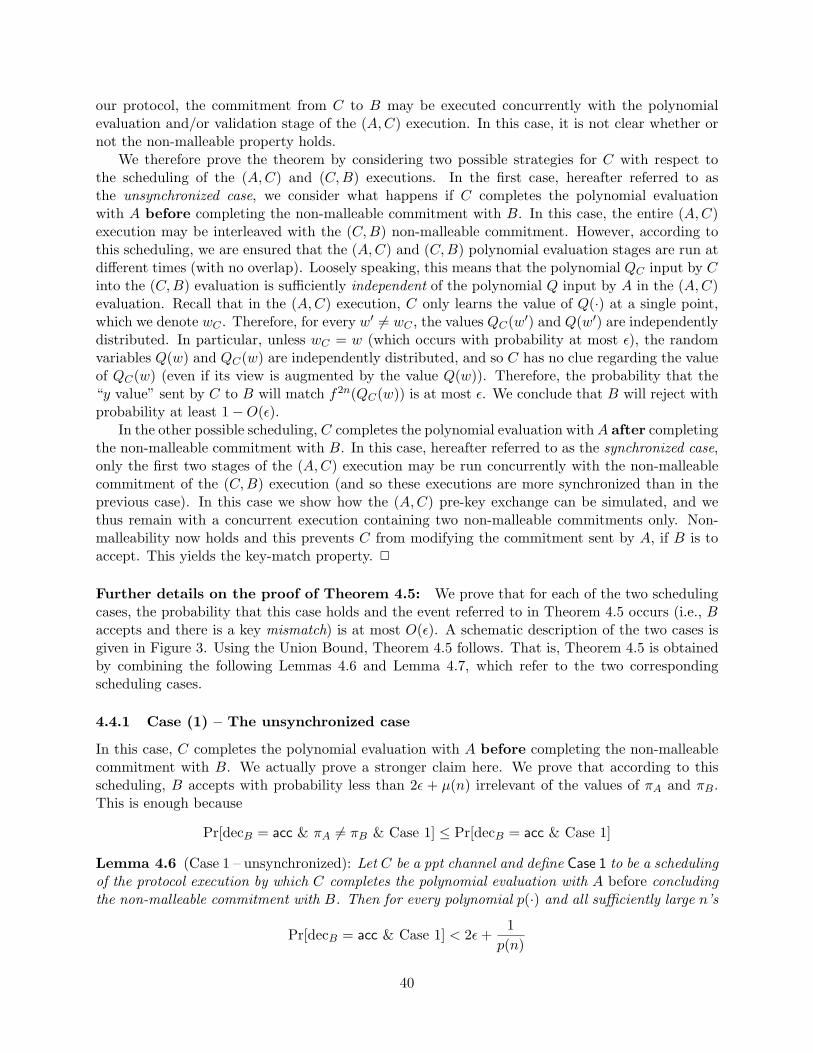
our protocol, the commitment from C to B may be executed concurrently with the polynomialevaluation and/or validation stage of the (A,C) execution. In this case, it is not clear whether ornot the non-malleable property holds.

We therefore prove the theorem by considering two possible strategies for C with respect tothe scheduling of the (A,C) and (C,B) executions. In the first case, hereafter referred to asthe unsynchronized case, we consider what happens if C completes the polynomial evaluationwith A before completing the non-malleable commitment with B. In this case, the entire (A,C)execution may be interleaved with the (C, B) non-malleable commitment. However, according tothis scheduling, we are ensured that the (A,C) and (C,B) polynomial evaluation stages are run atdifferent times (with no overlap). Loosely speaking, this means that the polynomial QC input by Cinto the (C, B) evaluation is sufficiently independent of the polynomial Q input by A in the (A,C)evaluation. Recall that in the (A,C) execution, C only learns the value of Q(·) at a single point,which we denote wC . Therefore, for every w′ 6= wC , the values QC(w′) and Q(w′) are independentlydistributed. In particular, unless wC = w (which occurs with probability at most ε), the randomvariables Q(w) and QC(w) are independently distributed, and so C has no clue regarding the valueof QC(w) (even if its view is augmented by the value Q(w)). Therefore, the probability that the“y value” sent by C to B will match f2n(QC(w)) is at most ε. We conclude that B will reject withprobability at least 1−O(ε).

In the other possible scheduling, C completes the polynomial evaluation with A after completingthe non-malleable commitment with B. In this case, hereafter referred to as the synchronized case,only the first two stages of the (A,C) execution may be run concurrently with the non-malleablecommitment of the (C,B) execution (and so these executions are more synchronized than in theprevious case). In this case we show how the (A,C) pre-key exchange can be simulated, and wethus remain with a concurrent execution containing two non-malleable commitments only. Non-malleability now holds and this prevents C from modifying the commitment sent by A, if B is toaccept. This yields the key-match property. 2

Further details on the proof of Theorem 4.5: We prove that for each of the two schedulingcases, the probability that this case holds and the event referred to in Theorem 4.5 occurs (i.e., Baccepts and there is a key mismatch) is at most O(ε). A schematic description of the two cases isgiven in Figure 3. Using the Union Bound, Theorem 4.5 follows. That is, Theorem 4.5 is obtainedby combining the following Lemmas 4.6 and Lemma 4.7, which refer to the two correspondingscheduling cases.

4.4.1 Case (1) – The unsynchronized case

In this case, C completes the polynomial evaluation with A before completing the non-malleablecommitment with B. We actually prove a stronger claim here. We prove that according to thisscheduling, B accepts with probability less than 2ε + µ(n) irrelevant of the values of πA and πB.This is enough because

Pr[decB = acc & πA 6= πB & Case 1] ≤ Pr[decB = acc & Case 1]

Lemma 4.6 (Case 1 – unsynchronized): Let C be a ppt channel and define Case 1 to be a schedulingof the protocol execution by which C completes the polynomial evaluation with A before concludingthe non-malleable commitment with B. Then for every polynomial p(·) and all sufficiently large n’s

Pr[decB = acc & Case 1] < 2ε +1

p(n)

40

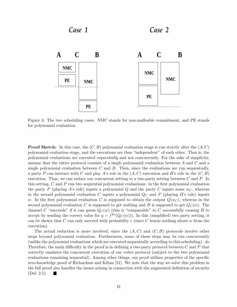
Case 1 Case 2

A C B A C B

NMC

PE NMC

PE

NMC

PE

NMC

Figure 3: The two scheduling cases. NMC stands for non-malleable commitment, and PE standsfor polynomial evaluation.

Proof Sketch: In this case, the (C, B) polynomial evaluation stage is run strictly after the (A,C)polynomial evaluation stage, and the executions are thus “independent” of each other. That is, thepolynomial evaluations are executed sequentially and not concurrently. For the sake of simplicity,assume that the entire protocol consists of a single polynomial evaluation between A and C and asingle polynomial evaluation between C and B. Then, since the evaluations are run sequentially,a party P can interact with C and play A’s role in the (A,C) execution and B’s role in the (C, B)execution. Thus, we can reduce our concurrent setting to a two-party setting between C and P . Inthis setting, C and P run two sequential polynomial evaluations: in the first polynomial evaluationthe party P (playing A’s role) inputs a polynomial Q and the party C inputs some wC , whereasin the second polynomial evaluation C inputs a polynomial QC and P (playing B’s role) inputsw. In the first polynomial evaluation C is supposed to obtain the output Q(wC), whereas in thesecond polynomial evaluation C is supposed to get nothing and B is supposed to get QC(w). Thechannel C “succeeds” if it can guess QC(w) (this is “comparable” to C successfully causing B toaccept by sending the correct value for y = f2n(QC(w))). In this (simplified) two party setting, itcan be shown that C can only succeed with probability ε (since C learns nothing about w from theexecution).

The actual reduction is more involved, since the (A,C) and (C,B) protocols involve othersteps beyond polynomial evaluation. Furthermore, some of these steps may be run concurrently(unlike the polynomial evaluations which are executed sequentially according to this scheduling). doTherefore, the main difficulty in the proof is in defining a two-party protocol between C and P thatcorrectly emulates the concurrent execution of our entire protocol (subject to the two polynomialevaluations remaining sequential). Among other things, our proof utilizes properties of the specificzero-knowledge proof of Richardson and Kilian [51]. We note that the way we solve this problem inthe full proof also handles the issues arising in connection with the augmented definition of security(Def. 2.5).

41

The full proof of Lemma 4.6 is presented in Section 6.1, and (as hinted above) is far more complexthan the above proof sketch.

4.4.2 Case (2) – The synchronized case

We now show that the probability that C completes the polynomial evaluation with A aftercompleting the non-malleable commitment with B and the bad event referred to in Theorem 4.5occurs (i.e., B accepts and there is a pre-key mismatch) is less than ε + µ(n).

Lemma 4.7 (Case 2 – synchronized): Let C be a ppt channel and define Case 2 to be a schedulingof the protocol by which C completes the polynomial evaluation with A after completing the non-malleable commitment with B. Then for every polynomial p(·) and for all sufficiently large n’s,

Pr[decB = acc & πA 6= πB & Case 2] < ε +1

p(n)

Proof Sketch: As we have mentioned, in this scheduling case we can show that the non-malleability property holds with respect to A’s commitment to the pair (Q,w). This is becausethe (C, B) non-malleable commitment is run concurrently only with the (A,C) non-malleable com-mitment and pre-key exchange. The main point is that the pre-key exchange can be simulatedusing only knowledge of Q (and without w).33 Therefore, we can give C the polynomial Q andreduce the scenario to one where the only protocols running are non-malleable commitments (asrequired by the definition of non-malleability). Given this, we have that the probability that Cwill commit to a pair (Q′, w′) where w′ = w is essentially the same as the probability of it guessingthe password w outright. (Recall that by the non-malleability of the commitment scheme, A’scommitment including the password w does not help C in generating a commitment that includesthe same w. This holds unless C simply copies A’s commitment unmodified; however, then we canshow that B rejects unless πA = πB, in which case key-match holds). We denote C’s non-malleablecommitment by (Q′, w′).

We first consider the probability that w′ = w (i.e., that the second element in the pair committedto by C equals the shared secret password of A and B), and Q′ 6= Q.34 Since A’s commitment doesnot help C in generating this commitment, and since w is uniformly distributed in D with respectto C’s view, the probability that C generates such a commitment (i.e., that w′ = w) is at mostnegligibly more than ε. (Indeed, if C generates a commitment with w′ = w, then it may cause Bto accept, even when πA 6= πB.)

Next, if B receives a non-malleable commitment to (Q′, w′) where w′ 6= w, then the validationstage ensures that B will reject. Essentially, this is because the (C, B) validation stage enforcesthat B’s output from the polynomial evaluation be consistent with the non-malleable commitmentthat B received. That is, it ensures that B will reject unless he receives Q′(w′) from the (C, B)-polynomial evaluation (i.e., πB = Q′(w′)). On the other hand, the validation stage also enforces

33This is the reason that an additional commitment to the polynomial Q is included in the pre-key exchange. Thatis, were we to augment the polynomial evaluation by having the parties include their transcripts of the non-malleablecommitment to Q and w (rather than just by a commitment to Q), then knowledge of w would be required forrunning A’s role in the pre-key exchange. The argument for non-malleability here would then fall.

34As we have mentioned, in case (Q′, w′) = (Q, w), we can show that party B rejects with overwhelming probability,unless πA = πB . This is because the validation stage essentially enforces that πB = Q′(w′), and therefore in case(Q′, w′) = (Q, w) it follows that πB = Q′(w′) = Q(w) = πA. Thus, in this proof sketch, we only consider the casethat (Q′, w′) 6= (Q, w).

42

that the polynomial input by C into the (C, B)-polynomial evaluation is Q′ (i.e., QC = Q′). Thus,the respective inputs of C and B into the (C, B)-polynomial evaluation are Q′ and w, and so Breceives Q′(w) as the output of this evaluation (by the evaluation’s correctness).35 Therefore, ifB accepts, it must be the case that Q′(w′) = Q′(w), which implies that w′ = w (because Q′ is anon-constant linear polynomial). Letting bad denote the event in the lemma’s claim, we get

Pr[bad] = Pr[bad & w′=w] + Pr[bad & w′ 6=w]≤ Pr[bad & w′=w & Q′=Q] + Pr[Case 2 & w′=w & Q′ 6=Q] + Pr[decB =acc & w′ 6=w]≤ µ(n) + (ε + µ(n)) + µ(n)

Referring to the augmented definition of security, we note that in this synchronization case, thesession-key challenge received by C in the augmented setting is of no consequence. This is becauseC completes its non-malleable commitment to B before A terminates, and so the value of itscommitment is determined before C receives the session-key challenge. Therefore, C’s success ingenerating a related commitment is independent of the session-key challenge. Furthermore, as isshown in the full proof, if C has failed in generating a related commitment, then B rejects withoverwhelming probability even if C is later given both Q and w (and not merely the session-keyk2(Q(w))).

The full proof of Lemma 4.7, which amounts to a careful implementation of the above proof sketch,can be found in Section 6.2.

4.5 Simulating the Stand-Alone (A, C) Execution

In this section, we show that C’s view, when interacting with A only, can be simulated by a machinethat interacts with nobody.36 Actually, we show that the joint distribution of C’s simulated viewalong with the password and a random string is (1 − O(ε))-indistinguishable from C’s real viewalong with the password and A’s output session-key.

Theorem 4.8 For every ppt channel C ′ interacting with A only, there exists a non-interactivemachine C ′′, such that

{w, k2(Q(w)), output(C ′A(Q,w)(σ))

}n,D,σ

2ε≡ {w, Un, output(C ′′(σ))

}n,D,σ

where Q is a random non-constant linear polynomial, D ⊆ {0, 1}n is any ppt samplable dictionary,w ∈R D, and ε = 1

|D| .

Proof Sketch: First, notice that it is enough to prove that for every ppt channel C ′,{w, k2(Q(w)), output(C ′A(Q,w)(σ))

}2ε≡

{w,Un, output(C ′A(Q,w)(σ))

}(13)

where w, w ∈R D are independently chosen passwords from D. In order to see that Eq. (13)implies Theorem 4.8, define the following non-interactive machine C ′′. Machine C ′′ chooses a

35Correctness, even in the concurrent setting, is implied by security in the stand-alone setting, because the latterholds even when the adversary knows the private input of the honest party, which in turn allows it to emulate theconcurrent execution.

36Recall that in the next subsection, we show that the (C, B)-execution can be simulated by C itself, while in-teracting with A. Thus put together, these two simulations provide the core of the proof of security of the entireprotocol (for active adversaries). Our choice of the current order of the two simulations is due to the fact that weuse elements in the analysis of the current simulation in the analysis of the next simulation.

43

random (linear, non-constant) polynomial Q and a “password” w ∈R D. Then, C ′′ perfectly em-ulates an execution of C ′A(Q,w)(σ) by playing A’s role (C ′′ can do this because it knows Q andw). Finally, C ′′ outputs whatever C ′ does. The resulting output of C ′′ is distributed exactlylike output(C ′A(Q,w)(σ)). Thus, it is enough to prove Eq. (13). Now, notice that the distribu-tions {w, Un, output(C ′A(Q,w)(σ))} and {w, Un, output(C ′A(Q,w)(σ))} are equivalent. We thereforeproceed by proving that

{w, k2(Q(w)), output(C ′A(Q,w)(σ))

}2ε≡

{w, Un, output(C ′A(Q,w)(σ))

}(14)

First we show that at the conclusion of the polynomial evaluation, with respect to C ′’s view, thepair (w, Q(w)) is (1−ε)-indistinguishable from (w, Un). The fact that w is indistinguishable from wfollows from the fact that in the first two stages of the protocol, A uses w only in the non-malleablecommitment. Thus, by the hiding property of the non-malleable commitment scheme, w remainsindistinguishable from w. It is therefore enough to show that after the polynomial evaluation thevalue of Q(w) is (1− ε)-pseudorandom, with respect to C ′’s view.

Consider what C ′ can learn about Q(w) from the first two stages of the protocol (i.e., until theend of the polynomial evaluation). Due to the hiding property of the two commitment schemes inuse, the two commitment transcripts reveal nothing of Q or w, and so the only place that C ′ canlearn something is from the polynomial evaluation itself. The security of the polynomial evaluationimplies that the receiver (here played by C ′) can learn nothing beyond the value of Q(·) at asingle point selected by C ′. We denote this point by wC . Thus, in the case that wC 6= w, givenQ(wC), the values Q(w) and Un are statistically close (recall that Q is a random, non-constant,linear polynomial and so we have “almost” pairwise independence). However, since w is uniformlydistributed in D (and C ′ learned nothing about it so far), the probability that wC = w is at mostε. This means that at the conclusion of the polynomial evaluation, with respect to C ′’s view, Q(w)can be distinguished from Un with probability at most negligibly greater than ε.

We have shown that after the first two stages, with respect to C ′’s view, (w, Q(w)) is (1 − ε)-indistinguishable from (w, Un). We now consider the messages sent by A in the remaining twostages. Recall that A sends nothing in the last (i.e., fourth) stage, whereas the only messagessent by A in the third stage are the value y = f2n(Q(w)), messages it sends as prover in thezero-knowledge proof, and a MAC of the entire message transcript keyed by k1(Q(w)). The zero-knowledge proof reveals nothing because it can be simulated by C ′ itself (in the standard manner,since here we are considering a stand-alone setting between A and C ′). Thus, it remains to dealwith y and the MAC-value. These are dealt with by showing that, even when given the valuey = f2n(Q(w)), the MAC-key k1(Q(w)), and the view of C ′ at the end of Stage 2, the value(w,Q(w)) is (1− 2ε)-indistinguishable from (w, Un). The latter implies Eq. (14), and is proven byrelying on the following two facts: (1) as established above, {w,Q(w)} is (1− ε)-indistinguishablefrom {w, Un}, with respect to C ′’s view at the end of Stage 2 of the protocol, and (2) the stringy = f2n(Q(w)) along with the MAC-key k1(Q(w)) and the session-key k2(Q(w)) constitutes apseudorandom generator. This concludes the proof of the theorem.

The full proof of Theorem 4.8, which amounts to a careful implementation of the above proofsketch, can be found in Section 7.

We note that since in this theorem we consider a stand-alone execution between A and C ′, theanalogous claim for the augmented definition of security holds as well. This is because the session-key challenge is only given to C ′ after the entire execution has terminated. Therefore, it is equivalentto giving the session-key to the distinguisher. However, the distinguisher receives the actual session-key anyway, and can thus generate the challenge by itself.

44

4.6 Simulating the (C, B) Execution

In this section, we show how the entire (C, B) execution can be simulated (by C while interactingwith A). That is, we consider the concurrent setting in which C interacts with both A and B. Weclaim that a channel interacting only with A can simulate C’s view in the concurrent setting withA and B, so that C’s simulated view is (1−O(ε))-indistinguishable from its view in an executionwith A and B. In fact, (1 − O(ε))-indistinguishability holds also for C’s view combined with thepassword and the session-key. That is,

Theorem 4.9 (simulating the (C, B) execution): For every ppt channel C interacting with A andB, there exists a ppt channel C ′ interacting only with A, such that

{w, k2(Q(w)), output(C ′A(Q,w)(σ))

}n,D,σ

5ε≡{w, k2(Q(w)), output(CA(Q,w),B(w)(σ))

}n,D,σ

where Q is a random non-constant linear polynomial, D ⊆ {0, 1}n is any ppt samplable dictionary,w ∈R D, and ε = 1

|D| .

Proof Outline: The theorem is proved in two steps. Conceptually, simulation of the (C, B)execution is demonstrated by separately showing how the first three stages of the (C,B) execution(i.e., everything except for B’s accept/reject bit) can be simulated, and then showing how B’saccept/reject bit itself can also be simulated. In order to implement this two-step process, weconsider a modified party B6dec that behaves exactly as B, except that it does not output anaccept/reject bit. Theorem 4.9 is obtained by combining the following Lemmas 4.10 and 4.11,which refer to the first and second steps, respectively. 2

Further details on the proof of Theorem 4.9: As outlined above, Theorem 4.9 is obtainedby combining Lemmas 4.10 and 4.11, which are stated in the following Subsections 4.6.1 and 4.6.2,respectively. In these subsections we also provide sketches for the proofs of these lemmas. The fullproofs, to be found in Section 8, are merely careful implementations of the corresponding proofsketches.

4.6.1 Step 1: Simulating the (C,B 6dec) execution

We start by showing that C’s interaction with A and the modified B (i.e., B 6dec, which has no publicaccept/reject output), can be simulated by a machine that only interacts with A.

Lemma 4.10 Let C be a ppt channel interacting with A and a modified party B 6dec who does notoutput an accept/reject bit. Then, there exists a ppt channel C ′ interacting with A only, such that

{w, k2(Q(w)), output(C ′A(Q,w))

}c≡

{w, k2(Q(w)), output(CA(Q,w),B 6dec(w))

}

Proof Sketch: Since k2(Q(w)) is a polynomial-time function of Q(w), it suffices to prove thefollowing equation:

{w, Q(w), output(C ′A(Q,w))

}c≡

{w, Q(w), output(CA(Q,w),B 6dec(w))

}(15)

First notice that the only messages sent by B6dec in the validation stage are as an honest verifierin the zero-knowledge proof. These can therefore be easily simulated. Next, observe that in the

45

remaining first two stages, the only place that B6dec uses w is in the (C, B 6dec) polynomial-evaluation.However, by the definition of the polynomial evaluation functionality, C receives no output fromthis evaluation and thus nothing is revealed about w. This is trivial in a stand-alone setting; here weclaim that it also holds in our concurrent setting. Formally, we show that if B6dec were to use somefixed w′ ∈ D instead of the password w, then this is indistinguishable to C (when also interactingconcurrently with A). That is, we show that for every ppt C,

{w, Q(w), output(CA(Q,w),B 6dec(w))

}c≡

{w,Q(w), output(CA(Q,w),B 6dec(w

′))}

(16)

where w ∈R D is a random password and w′ ∈ D is fixed. This is shown by reducing C’s concurrentexecution with A and B 6dec to a stand-alone two-party setting between C and B6dec only.37 Thereduction is obtained by providing C with the password w and the polynomial Q, which enablesC to perfectly emulate the entire (A, C) execution. As a result of this emulation, we are left witha stand-alone setting between C and B 6dec in which B6dec inputs either w or w′ into the polynomialevaluation (and C knows both w and w′). In this stand-alone setting, the security of the polynomialevaluation guarantees that C can distinguish the input cases with at most negligible probability,even when given both w and w′ (as well as Q). Eq. (16) follows.

We have established that C cannot distinguish the case that B6dec uses w from the case thatB6dec uses w′. This suggests to define the channel C ′ as follows: C ′ chooses an arbitrary w′ ∈ Dand emulates the CA(Q,w),B 6dec(w

′) setting for C, while interacting with A(Q,w) (and using w′ in theemulation of B 6dec(w′)). At the end of the interaction, C ′ outputs whatever C does. Channel C’sview in this simulation is indistinguishable from in a real execution with A and B6dec, establishingEq. (15) and therefore proving the lemma.

We note that the above argument is unchanged when considering the augmented definition ofsecurity. This is true because Eq. (16) holds even if C is explicitly given both Q and w (in whichcase C can generate the session-key challenge by itself).

4.6.2 Step 2: Simulating B’s decision bit

We now show how the accept/reject bit of B can be simulated (while interacting with A and B 6dec).This modification of B to B6dec is straightforward when considering Definition 2.4. However, forthe augmented definition (Def. 2.5) we must also say how the session-key challenge is generated(because by the definition of the augmented real-model, this value depends on whether or notthe first party concluding accepts or rejects). Now, if A concludes first, then nothing is changed.However, if B 6dec concludes first, then we set the challenge session-key to always equal ⊥. We nowproceed to the simulation:

Lemma 4.11 Let B6dec be a party who does not output an accept/reject bit. Then, for every pptchannel C interacting with A and B, there exists a ppt channel C interacting with A and B6dec,such that

{w, k2(Q(w)), output(CA(Q,w),B 6dec(w))

}5ε≡

{w, k2(Q(w)), output(CA(Q,w),B(w))

}

37Indeed, the reader may consider this reduction (i.e., removing the (A, C) execution) odd, given that our finalgoal here is to remove the (C, B 6dec) execution (i.e., reduce C’s concurrent execution with A and B 6dec to a stand-alonetwo-party setting between C and A). Still, such a reduction enables us to establish Eq. (16), and once Eq. (16) isestablished we proceed to remove the (C, B 6dec) execution.

46

Proof Sketch: The proof of this claim relies heavily on the security of the MAC-value sent inthe validation stage of the protocol. Recall that A sends a MAC of her entire session-transcriptusing k1(πA) = k1(Q(w)) as the key. Furthermore, B verifies the MAC value that it receives usingthe key k1(πB), where πB is B’s output from the polynomial evaluation. Intuitively, the MACensures that, except with probability O(ε), if C was not reliable, then B will detect its interferenceand will therefore reject. On the other hand, if C was reliable then B will surely accept. Looselyspeaking, this means that C can learn “at most an O(ε) fraction of a bit of information” from B’saccept/reject bit.

We begin by proving the security of the MAC value when keyed by k1(πA). This is an importantstep in proving Lemma 4.11. We note that we need to show that the MAC is secure only beforeB outputs its accept/reject bit. Thus, we consider a scenario in which C interacts with A andthe modified party B6dec. The security of the MAC is formally stated in the following claim. (Forsimplicity, we consider an implementation of a MAC by a pseudorandom function. However, ourproof can be extended to any secure implementation of a MAC.)

Claim 4.12 Let C be an arbitrary ppt channel interacting with A and a modified party B6dec as inLemma 4.11, and let tA and tB denote the transcripts from the (A,C) and (C, B6dec) executions,respectively. Then, if tA 6= tB, it holds that the value MACk1(πA)(tB) is (1 − 2ε)-pseudorandomwith respect to C’s view. That is, for every probabilistic polynomial-time distinguisher D, everydictionary D ⊆ {0, 1}n, every auxiliary-input σ and all sufficiently large n’s

∣∣∣Pr[D(MACk1(πA)(tB), CA(Q,w),B 6dec(w)) = 1 & tA 6= tB]

−Pr[D(Un, CA(Q,w),B 6dec(w)) = 1 & tA 6= tB]∣∣∣ < 2ε + µ(n)

Proof Sketch: We first observe that we can ignore the entire (C, B6dec) execution in provingthe claim. A similar claim has already been shown in Lemma 4.10 (above). Loosely speaking,Eq. (15) in the proof of Lemma 4.10 states that C’s view is essentially the same when interactingwith A and B 6dec or when interacting with A alone. Actually, Eq. (15) asserts that these twoviews are indistinguishable also when considered in conjunction with (w, Q(w)). Since k1(·) is apolynomial-time function, it follows that these two views are indistinguishable also when consideredin conjunction with (w, k1(Q(w)), where k1(Q(w)) is the MAC-key.

We now analyze the security of the MAC-key in a stand-alone setting between A and C. Thisproof is very similar to the proof of Theorem 4.8 (there k2(Q(w)) is shown to be (1 − O(ε))-pseudorandom; here a similar result is needed with respect to k1(Q(w))). As in Theorem 4.8, wefirst establish that at the conclusion of the polynomial evaluation, the value Q(w) is (1 − O(ε))-pseudorandom to C. Next, recall that the only messages sent by A in the third stage of theprotocol are y = f2n(Q(w)), messages from a zero-knowledge proof and a MAC of the messagetranscript. The zero-knowledge proof can be simulated and so it reveals nothing. Then, sinceG(s) = (f2n(s), k1(s)) is a pseudorandom generator and Q(w) is (1 − O(ε))-pseudorandom at theend of Stage 2, it holds that the MAC-key k1(Q(w)) remains (1−O(ε))-pseudorandom even giveny = f2n(Q(w)).

Having established that the MAC-key is (1− O(ε))-pseudorandom (with respect to C’s view),we conclude by showing that this implies that the probability that C successfully forges the MACis at most O(ε)+µ(n). Now, since k1(Q(w)) is (1−O(ε))-pseudorandom, a pseudorandom functionkeyed by k1(Q(w)) is also (1 − O(ε))-pseudorandom. Recall that the last message sent by Ais MACk1(Q(w))(tA) where tA is A’s message transcript. Therefore, by the properties of a (1 −O(ε))-pseudorandom function, for every t 6= tA that C can produce, the value MACk1(Q(w))(t) is

47

(1 − O(ε))-pseudorandom given C’s view. Since tB is part of C’s view, it follows that the valueMACk1(Q(w))(tB) is (1−O(ε))-pseudorandom given C’s view. This concludes the proof of the claim.

We note that the above also holds for the augmented definition of security. This is becausethe MAC-key k1(Q(w)) remains (1−O(ε))-pseudorandom even given both y = f2n(Q(w)) and thesession-key k2(Q(w)). Therefore, even if the session-key challenge equals k2(Q(w)), this cannothelp C generate a correct MAC. Given that this is the case, the rest of the proof also follows forthe augmented definition.

We now use Claim 4.12 and Theorem 4.5 (the key-match property) to show that the probabilitythat B accepts in executions for which C is not reliable is at most O(ε). (Recall that C is reliablein a particular execution if it acts like a passive (eavesdropping) adversary in that execution.)

Proposition 4.13 For every ppt channel C,

Pr[decB = acc & reliableC = false] < 5ε + µ(n)

Proof Sketch: We show this proposition by combining the following facts:• Theorem 4.5 states that the probability that B accepts and πA 6= πB is at most negligibly

greater than 3ε.

• Let tA and tB be the (A,C) and (C, B) message-transcripts, respectively. Then, Claim 4.12states that if tA 6= tB, then MACk1(πA)(tB) is (1− 2ε)-pseudorandom with respect to C’s view.

• B only accepts if he receives MACk1(πB)(tB) (i.e., a MAC value keyed by k1(πB)) in the laststep of the protocol.

Now, consider the case that C is not reliable and thus by definition tA 6= tB. Then, if πA = πB wehave that, by the security of the MAC, party B accepts with probability at most negligibly morethan 2ε. On the other hand, if πA 6= πB, then by the key-match property, party B accepts withprobability at most 3ε (irrespective of the MAC). Therefore, the probability that B accepts andtA 6= tB is at most negligibly greater than 5ε.

Given Proposition 4.13, we can complete the proof of Lemma 4.11. First, we describe the adversaryC (who interacts with A and B 6dec). Channel C emulates an execution of CA(Q,w),B(w), whileinteracting with A and B6dec. This emulation is “easy” for C, except for the accept/reject decisionbit of B (since this is the only difference between its execution with A and B6dec, and an executionwith A and B). Therefore, at the conclusion of the (C, B 6dec) execution, C attempts to guess B’saccept/reject decision-bit (which is not given to C but which C does expect to see) and outputswhatever C does. Channel C’s guess for B’s decision-bit is according to the natural rule (suggestedby the above discussion): B accepts if and only if C was reliable. We stress that C can easilydetermine whether or not C was reliable (in the current execution). To establish the approximate-correctness of the above rule, observe that, on one hand, if C is reliable then B always accepts(and so, in this case, C’s guess is always correct). On the other hand, if C was not reliable, thenB accepts with probability at most 5ε + µ(n). Therefore, C is wrong in its guess with probabilityat most 5ε + µ(n), and the difference in C’s view in the case that it really receives B’s output bitand the case it receives C’s guess, is at most negligibly greater than 5ε.

We note this simulation by C is also easily carried out under the augmented definition. Thisis the case because if C was reliable, then A must have finished first, and so there is no differ-ence between the challenge session-key received by C in CA(Q,w),B 6dec(w) and that received by C in

48

CA(Q,w),B(w). On the other hand, if B6dec finished first in its execution with C, then C must havebeen not reliable in the emulation of CA(Q,w),B(w) by C. Therefore, except with probability 5ε, thechallenge session-key received by C would equal ⊥, which is the same as what C receives in themodified execution with B6dec.

4.7 The Security of Protocol 3.2 for Arbitrary Adversaries

The fact that Protocol 3.2 satisfies Definition 2.4 (i.e., Theorem 3.3) follows by combining thepassive adversary case (i.e., Theorem 4.1) and the active adversary case (i.e., Theorem 4.14, below).

Theorem 4.14 (active executions): Protocol 3.2 satisfies Condition 2 in Definition 2.4. That is,for every ppt real-model channel C, there exists a ppt ideal-model channel C, such that

{idealC(D, σ)

}n,D,σ

12ε≡ {realC(D, σ)}n,D,σ

where D ⊆ {0, 1}n is any ppt samplable dictionary, σ ∈ {0, 1}poly(n) is the auxiliary input for theadversary, and ε = 1

|D| .

In this section, we present a full proof of Theorem 4.14. Our main tools are the simulations providedby Theorems 4.8 and 4.9 (presented in Sections 4.5 and 4.6, respectively). In addition, we make anessential use of Proposition 4.13 (of Section 4.6), and a marginal use (i.e., in order to save an O(ε)term) of Proposition 4.3 (of Section 4.3).

Proof: We begin by describing the ideal-model channel C. Adversary C is derived from thetransformations of Theorems 4.8 and 4.9. That is, combining these theorems together, we havethat for every ppt real-model channel, there exists a non-interactive machine C ′′ such that

{w, Un, output(C ′′(σ))

} 7ε≡{w, k2(Q(w)), output(CA(Q,w),B(w)(σ))

}(17)

Next, we define the ideal-model channel C as follows: C first invokes the non-interactive machineC ′′ guaranteed by Eq. (17). When C receives the output of C ′′ (which contains C’s view and inparticular B’s accept/reject bit), C sets the value of b (the bit sent by it to the trusted party) asfollows:• If B accepted in the view output by C ′′, then C sends b = 1 to the trusted party.

• If B rejected in this view, then C sends b = 0 to the trusted party.(Recall that upon receiving b = 1, the trusted party hands the same uniformly distributed key to Aand B. On the other hand, upon receiving b = 0, the trusted party hands a uniformly distributedkey to A, and B receives ⊥.) Finally, C halts and outputs the output of C ′′.

Before proceeding, we remark on an important property regarding the simulated view of C thatis output by C ′′. In this view, B accepts if and only if C was reliable. This is because this is the waythat B’s accept/reject bit is simulated by C, as described at the end of the proof of Lemma 4.11.We will use this property below.

We now show that the combined input/output distributions in the real and ideal models are atmost negligibly greater than 12ε apart. By Eq. (17) and the definition of C, we have that

{w, Un, output(C)

}7ε≡

{w, k2(Q(w)), output(CA(Q,w),B(w))

}(18)

49

This seems very close to proving the theorem (the first distribution is “almost” the ideal-modeldistribution and the second distribution is “almost” the real-model distribution), where in bothcases the only thing missing is B’s local output (which may or may not equal A’s local output).included). It remains to show that the distributions are still (1−O(ε))-indistinguishable even whenB’s output is included. Loosely speaking, this is shown by separately considering the cases thatC acts reliably and unreliably. When C is reliable, then the ideal and real distributions arecomputationally indistinguishable (by Proposition 4.3). On the other hand, when C is not reliable,then B rejects with probability at least 1− 5ε, in which case B’s output is defined as ⊥.

Formally, let D be any ppt distinguisher who attempts to distinguish between the ideal andreal distributions. We separately analyze the distance between the distributions when B acceptsand when B rejects. When referring to B’s decision (i.e., decB), within the context of idealC , wemean B’s decision as included in the emulated view of C (which is part of the output of C). (Notethat by the construction of C, it holds that B’s decision in the emulated view matches the outputof B in the ideal-model; i.e., decB = rej iff the output of B in the ideal-model is ⊥.) We begin withthe case that B rejects:

∣∣Pr[D(idealC(D, σ)) = 1 & decB = rej]− Pr[D(realC(D, σ)) = 1 & decB = rej]∣∣

=∣∣∣Prw

[D

(w, Un,⊥, output(C)

)= 1 & decB = rej

]

− PrQ,w

[D

(w, k2(Q(w)),⊥, output(CA(Q,w),B(w))

)= 1 & decB = rej

]∣∣∣

The above follows from the protocol definition that states that when B rejects it outputs ⊥, andfrom the construction of the ideal-model adversary C who sends b = 0 to the trusted party (causingB’s output to be ⊥) in the case that B rejects in the view output by C ′′. Noting that C’s viewincludes B’s accept/reject decision bit (and thus implicitly B’s output of ⊥ in the case that Brejects), by Eq. (18) we have that

∣∣Pr[D(idealC(D, σ)) = 1 & decB = rej]−Pr[D(realC(D, σ)) = 1 & decB = rej]| < 7ε + µ(n) (19)

We now analyze the case that B accepts. Here, we further break down the events and separatelyconsider the case that C is reliable and C is not reliable. (Recall that in the ideal distribution, theevent of C being reliable or not refers to its behavior as implicit in the view output by C ′′ for C.)Starting with the subcase in which C is reliable, we have:∣∣Pr[D(idealC(D, σ)) = 1 & decB = acc & reliableC = true]

− Pr[D(realC(D, σ)) = 1 & decB = acc & reliableC = true]|=

∣∣∣Prw

[D

(w,Un, Un, output(C)

)= 1 & decB = acc & reliableC = true

]

− PrQ,w

[D

(w, k2(Q(w)), k2(Q(w)), output(CA(Q,w),B(w))

)= 1 & decB = acc & reliableC = true

]∣∣∣

Noting that when C is reliable, B always accepts (and so its real-model and ideal-model outputsare always k2(Q(w)) and Un respectively), we have that the above difference equals

∣∣Pr[D(realC(D, σ)) = 1 & reliableC = true]− Pr[D(idealC(D, σ)) = 1 & reliableC = true]∣∣

By Proposition 4.3 this difference is at most negligible. We now consider the case in which Baccepts and C is not reliable.

∣∣Pr[D(idealC(D, σ)) = 1 & decB = acc & reliableC = false]− Pr[D(realC(D, σ)) = 1 & decB = acc & reliableC = false]|

50

By Proposition 4.13 we have that in a real execution, Pr[decB = acc & reliableC = false] < 5ε+µ(n).In contrast, in an ideal execution, Pr[decB = acc & reliableC = false] = 0. This is due to the factthat in the simulated transcript output by C ′′, party B accepts if and only if C was reliable (asmentioned above). Therefore, we have that the above difference is at most negligibly greater than5ε. Putting these together, we have that

∣∣Pr[D(idealC(D, σ)) = 1 & decB = acc]−Pr[D(realC(D, σ)) = 1 & decB = acc]| < 5ε + µ(n) (20)

Combining Equations (19) and (20) we conclude that,∣∣Pr[D(idealC(D, σ)) = 1]− Pr[D(realC(D, σ)) = 1]

∣∣ < 12ε + µ(n)

and the theorem follows.

5 Full Proof of Security for Passive Adversaries

In this section, we present the proof of Lemma 4.2, used for proving the “passive adversaries”requirement of Definition 2.4. Recall that this lemma relates to a passive channel C who can onlyeavesdrop on protocol executions between honest parties A and B. This means that C receives thetranscript of messages sent by A and B and tries to “learn something” based on this transcriptalone.

Lemma 5.1 (Lemma 4.2 – restated): For every passive ppt channel C,{w, k2(Q(w)), output(CA(Q,w),B(w))

}c≡

{w,Un, output(CA(Q,w),B(w))

}

where Q is a random non-constant linear polynomial, and w and w are independently and uniformlydistributed in D.

Proof: As we have mentioned, since C is passive, it merely receives a message transcript of atwo-party protocol. We stress that there are no concurrent adversarial executions in this case, butrather merely a transcript of a standard stand-alone protocol execution between two honest parties.The issue is merely what can a third party (i.e., C) learn from such a transcript. We answer thisquestion by relying on the (stand-alone) security of the different modules in our protocol. We startby presenting notation for transcripts of executions of our protocol.

The message-transcript of an execution of our protocol is a function of the inputs Q and w, andthe respective random coins of A and B, denoted rA and rB. We denote the message transcriptof the first two stages of the protocol by t2(Q, w, rA, rB). Furthermore, we denote by T2(Q,w)a random variable that assumes values of t2(Q,w, rA, rB) where rA and rB are randomly chosen.(Note that the security parameter n, and thus the lengths of Q,w,rA and rB are implicit in all thesenotations.)

We begin by showing that the probability ensemble {T2(Q1, w1)}Q1,Q2,w1,w2 is computationallyindistinguishable from {T2(Q2, w2)}Q1,Q2,w1,w2 .

38 This is proved in the following claim, which isthen used to establish the lemma (which refers to the entire protocol execution, rather than justto the first two stages as shown in the claim).

38Notice that it is not true that the ensembles {T (Q1, w1)}Q1,Q2,w1,w2 and {T (Q2, w2)}Q1,Q2,w1,w2 are indistin-guishable, where T (Q, w) is a random variable assuming message transcripts for the entire protocol (including thevalidation stage). This is because the string y = f2n(Q(w)) is sent during the validation stage. Thus, given (Q1, w1), adistinguisher may compare f2n(Q1(w1)) to the y-value of the transcript, and determine whether or not the transcriptis based on (Q1, w1).

51

Claim 5.2 The probability ensemble {T2(Q1, w1)}Q1,Q2,w1,w2 is computationally indistinguishablefrom {T2(Q2, w2)}Q1,Q2,w1,w2. That is, for every non-uniform ppt distinguisher D, every polynomialp(·) and all sufficiently large pairs (Q1, w1) and (Q2, w2),

|Pr[D(t2(Q1, w1, rA, rB)) = 1]− Pr[D(t2(Q2, w2, rA, rB)) = 1]| < 1p(n)

where rA and rB are uniformly chosen strings.

Proof: The proof is based on the security of the different modules in the protocol.

The Commitments: Due to the hiding property of string commitments, a non-malleable commit-ment to (Q1, w1) is indistinguishable from one to (Q2, w2), and likewise an ordinary commitmentto Q1 is indistinguishable from one to Q2.

The Polynomial Evaluation: The inputs to the polynomial evaluation are Q,w and Commit(Q).Denote by TP (Q,w), a random variable assuming transcripts for this evaluation (when the partiesA and B use uniformly distributed random tapes). We claim that for all sufficiently large valuesof Q1, Q2, w1, w2, we have that {TP (Q1, w1)} and {TP (Q2, w2)} are indistinguishable. This can bederived from the following two facts (and is based on the security of the polynomial evaluation thatimplies that A learns nothing and that B learns only Q(w)):

1. For all sufficiently large non-constant, linear polynomials Q, passwords w ∈ D and stringsx ∈ {0, 1}n, we have that

{TP (Q,w)}Q,w,xc≡ {TP (Q, x)}Q,w,x (21)

This is based directly on the fact that A learns nothing of B’s input (which is either wor x) from the evaluation. Therefore, given her message transcript, A must not be able todistinguish the case that B used w from the case that B used x. Eq. (21) follows.

2. For all sufficiently large non-constant, linear polynomials Q1, Q2 and strings x ∈ {0, 1}n suchthat Q1(x) = Q2(x), it holds that

{TP (Q1, x)}Q1,Q2,xc≡ {TP (Q2, x)}Q1,Q2,x (22)

This is because B obtains only Q(x) from the evaluation, where A inputs Q ∈ {Q1, Q2}.Since Q1(x) = Q2(x), party B cannot distinguish the case that A inputs Q1 or Q2 into theevaluation (otherwise he learns more than just Q(x)). Eq. (22) follows.

Now, for every two non-constant polynomials Q1 and Q2, there exists a third polynomial Q3 andvalues x1 and x2 such that Q1(x1) = Q3(x1) and Q2(x2) = Q3(x2). Therefore, we have that for allsufficiently large non-constant linear polynomials Q1, Q2 and passwords w1, w2 ∈ D

{TP (Q1, w1)} c≡ {TP (Q1, x1)}c≡ {TP (Q3, x1)}c≡ {TP (Q3, x2)}c≡ {TP (Q2, x2)}c≡ {TP (Q2, w2)}

52

where Q3, x1, x2 are as described above (the ensembles in the above equations are indexed by(Q1, Q2, Q3, w1, w2, x1, x2)). The first, third and fifth “

c≡” are due to Eq. (21) and the second andfourth is from Eq. (22). We therefore have that {TP (Q1, w1)} c≡ {TP (Q2, w2)}. Combining thiswith what we have shown regarding the commitments, the claim follows.

Loosely speaking, the above claim shows that the transcript of the first two stages of the protocolreveals nothing significant about the polynomial or password used in the execution. Recalling thatno messages are sent in the last (fourth) stage, it remains to analyze the additional messages sentin the third stage of the protocol. Recall that the third stage (validation) consists of A sendingy = f2n(Q(w)), a zero-knowledge proof, and a MAC of the session-transcript keyed by k1(Q(w)). Tosimplify the exposition, we will assume that A sends the MAC-key itself, rather than the MAC-value(which can be computed by C from the MAC-key and the visible session-transcript). Intuitively, thezero-knowledge proof reveals nothing, and the session-key k2(Q(w)) remains pseudorandom evengiven f2n(Q(w)) and k1(Q(w)) because G(Q(w)) def=

(f2n(Q(w)), k1(Q(w)), k2(Q(w))

)constitutes

a pseudorandom generator. Furthermore, the password w is “masked” by Q, and therefore remainssecret, even given Q(w) itself. Details follow.

By the definition of zero-knowledge, there exists a simulator that generates proof-transcriptsindistinguishable from real proofs. Thus, we may ignore this part of the validation stage for the restof the proof (because, using the simulator, C may generate this part by itself). Thus, we may assumethat the entire session-transcript consists of T2(Q,w) along with the pair

(f2n(Q(w)), k1(Q(w))

).

From here on, we denote by {T2(Q,w), Q, w)}n,D (and variations of this), a probability ensemblewhere Q and w are chosen randomly and then the transcript T2 is generated based on this Q and w.(Previously, the ensembles considered here were indexed by Q and w; from here on, the ensemblesare indexed by n and D.) Thus, in order to complete the proof of the lemma, it remains to showthat for randomly chosen values Q1, Q2, w1, w2,

{T2(Q1, w1), f2n(Q1(w1)), k1(Q1(w1)), k2(Q1(w1)), w1}n,Dc≡ {T2(Q2, w2), f2n(Q2(w2)), k1(Q2(w2)), Un, w1}n,D (23)

Now, using Claim 5.2 and the fact that for a random Q1, the value Q1(w1) is uniformly distributedin {0, 1}n (for every w1), we have

{T2(Q1, w1), Q1(w1), w1}n,Dc≡ {T2(Q2, w2), Q1(w1), w1}n,D

c≡ {T2(Q2, w2), Un, w1}n,D (24)

(Notice that Q1 is independent of T2(Q2, w2).) This then implies that

{T2(Q1, w1), f2n(Q1(w1)), k1(Q1(w1)), k2(Q1(w1)), w1}n,Dc≡ {T2(Q2, w2), f2n(Un), k1(Un), k2(Un), w1}n,Dc≡ {T2(Q2, w2), f2n(U (1)

n ), k1(U (1)n ), U (2)

n , w1}n,D (25)

where the last “c≡” is by pseudorandomness of the generator G(s) =

(f2n(s), k1(s), k2(s)

), and U

(1)n

and U(2)n denote independent uniform distributions over n-bit strings. Using Eq. (24), we have

{T2(Q2, w2), Un}n,Dc≡ {T2(Q1, w1), Q1(w1)}n,D ≡ {T2(Q2, w2), Q2(w2)}n,D

and since w1 ∈R D independently of (Q2, w2), it holds that

{T2(Q2, w2), U (1)n , w1}n,D

c≡ {T2(Q2, w2), Q2(w2), w1}n,D

53

This, in turn, implies that

{T2(Q2, w2), f2n(U (1)n ), k1(U (1)

n ), U (2)n , w1}n,D

c≡ {T2(Q2, w2), f2n(Q2(w2)), k1(Q2(w2)), U (2)n , w1}n,D

(26)Combining Equations (25) and (26), we obtain Eq. (23) completing the proof of the lemma (byreplacing w1 with w and w2 with w in Eq. (23), this is the same as the lemma statement).

6 Full Proof of the Key-Match Property

The key-match property captured in Theorem 4.5 states that the probability that A and B bothaccept, yet have different pre-keys (i.e., πA 6= πB) is at most O(ε). Recall that πA

def= Q(w) andthat πB is B’s output from the polynomial evaluation. We prove this theorem by considering twocomplementary schedulings of the concurrent executions. We show that for each scheduling, theprobability that B accepts and πA 6= πB is at most O(ε). (In fact, in the first scheduling, B acceptswith probability at most O(ε), irrespective of whether or not πA = πB.)

6.1 Proof of Lemma 4.6 (The Unsynchronized Case)

The proof of Lemma 4.6 will involve considering a variety of different settings. Specifically, we willconsider the probability that B accepts when interacting with C, which in turn interacts with apair of machines that are not necessarily A and B. For sake of clarity, we introduce the notationdec(CA′,B′) that means the decision of B′ (which is public and known to C) when interacting withC that interacts concurrently also with A′.

Lemma 6.1 (Lemma 4.6 – restated; Case 1 – unsynchronized): Let C be a ppt channel and defineCase 1 to be a scheduling of the protocol execution by which C completes the polynomial evaluationwith A before concluding the non-malleable commitment with B. Then, for every polynomial p(·)and all sufficiently large n’s

Pr[dec(CA,B) = acc & Case 1] < 2ε +1

p(n)

Proof: The proof of this lemma is the most complex proof in this paper. It proceeds by reducing theconcurrent setting to a two-party stand-alone setting. However, before performing this reduction,we “remove” the zero-knowledge proofs from the protocol. This is done in two steps: a smallstep in which the zero-knowledge proof in which B plays the verifier is removed (from the (C, B)interaction), and a big step in which the zero-knowledge proof in which A plays the prover isremoved (from the (A,C) interaction).

We start with the small step. We consider a modified party, denoted B′, that accepts or rejectsbased solely on the y-value received in the validation stage. That is, B′ does not play the verifier inthe zero-knowledge proof given by C, and also ignores the MAC sent by C. Since we only omittedchecks that may make B reject, we have that

Pr[dec(CA,B) = acc & Case 1] ≤ Pr[dec(CA,B′) = acc & Case 1] (27)

The proof of the lemma proceeds by showing that the r.h.s is upper-bounded by 2ε + µ(n). Westress that (by considering B′ rather than B) we have removed the zero-knowledge proof given byC to B, but the zero-knowledge proof given by A to C still remains. The next subsection is devoted

54

to getting rid of the latter proof, which is the big step (mentioned above). Once this is achieved,we turn (in Subsection 6.1.2) to analyzing the residual protocol, by reducing the analysis of itsexecution in the concurrent three-part setting to an analysis of an auxiliary two-party protocol inthe standard stand-alone setting.

6.1.1 Simulating A’s zero-knowledge proof

We begin by showing that when C interacts with A and B′, the zero-knowledge proof given by Ato C can be simulated. Since the proof (given by A to C) is zero-knowledge, it seems that thechannel C (who plays the verifier in the proof) should be able to simulate it itself. This is true (bydefinition) if the zero-knowledge proof is executed as stand-alone. However, the definitions of zero-knowledge guarantee nothing in our setting, where the proof is run concurrently with other relatedprotocols (belonging to the (C,B′)-execution). Technically speaking, the zero-knowledge simulationof A typically requires rewinding C. However, messages belonging to the (C, B′)-execution may beinterleaved with the proof. For example, C’s queries to A in the proof may depend on messagesreceived from B′. Rewinding C would thus also require rewinding B′. However, since B′ is anexternal party, he cannot be rewound.

We remark that concurrent zero-knowledge does not solve this problem either, since it relatesto concurrent executions of a (zero-knowledge) protocol with itself, and not concurrently witharbitrary protocols. Still, we use the ideas underlying the concurrent zero-knowledge proof systemof Richardson and Kilian [51] in order to address the problem that arises in our application.

We refer the reader to Appendix A.4 for a description of the Richardson and Kilian (RK) proofsystem. Recall that we set the parameter m (the number of iterations in the first part of the RKproof) to equal r+t(n), where r is the total number of rounds in the first two stages of our protocol,and t(n) is any non-constant function of the security parameter n (e.g., t(n) = log log n).

We now motivate how the proof simulation is done in our scenario, where C interacts with Aand B′. In such a case (when B′ rather than B is involved), the total number of rounds in the(C,B′) execution equals r = m− t (since B′ does not participate in the zero-knowledge proof givenby C in the validation stage). On the other hand, the number of iterations in the first part of theRK-proof given by A to C equals m. Therefore there are t complete iterations in the first partof this proof in which C receives no messages from B′. In these iterations it is possible to rewindC without rewinding B′. This is enough to establish zero-knowledge, since the Richardson-Kilianconstruction is such that as soon as rewinding is possible in one iteration, the entire proof may besimulated. The crucial point is that we rewind C at a place that does not require the rewinding ofB′ (which is not possible, since B′ is an outside party). With this motivation in mind, we move toour actual proofs.

The modification of A into A6zk. In our above description, when we say that A’s proof can besimulated by C itself, this means that A can be modified to a party A6zk, whose protocol definitiondoes not include providing a zero-knowledge proof in the validation stage. Before continuing, weformally define what we mean by this modification of A to A6zk. This needs to be done carefullybecause the transcript (and not just the result) of the zero-knowledge proof affects other parts ofour protocol. Specifically, in the validation stage, A sends a MAC of her entire message-transcriptto C. This message-transcript includes also the messages of the zero-knowledge proof. Therefore,the protocol of A6zk must be appropriately redefined to take this issue into account.

In the zero-knowledge proof with C, party A plays the prover. The essence of the modificationof A to A6zk is in replacing A’s actions as prover in the (A,C)-proof by C simulating the resulting

55

messages by itself. This modification works only if C’s view in the protocol execution with A6zk isindistinguishable from its view in an execution with A. As mentioned, the MAC sent by A in thevalidation stage refers to the entire message transcript, including messages from the zero-knowledgeproof. Therefore, the MAC value sent by A6zk must also include messages from the simulated proof.However, A6zk does not see these messages as the simulation is internal in C; therefore the messagetranscript of the proof must be explicitly given to her.

In light of this discussion, we define the modified A6zk to be exactly the same as A, exceptthat she does not provide a zero-knowledge proof (in her validation stage). Instead, at the pointin which A’s zero-knowledge proof takes place, she receives a string s that she appends to hermessage transcript. This means that the only difference between A and A6zk’s message transcriptsis that A’s transcript includes messages from a zero-knowledge proof and A6zk’s transcript includess instead. Intuitively, if s is the transcript of the simulated proof, then A and A6zk’s messagetranscripts are indistinguishable. This ensures that the MACs sent by A and A6zk, respectively, areindistinguishable.

The simulation. We now show that for every channel C interacting with A and B′, there existsa channel C ′ interacting with A6zk and B′ such that the channels’ views in the two cases areindistinguishable. Since B’s accept/reject bit is part of C’s view (which is included in C’s output),it follows that the probability that B′ accepts (in an execution with C ′ and A6zk) is negligibly closeto the probability that B′ accepts (in an execution with C and A). This enables us to continueproving Lemma 6.1 by considering the setting where C interacts with A6zk and B′ (rather than withA and B′).

Lemma 6.2 Let A6zk and B′ be as above. Then, for every ppt channel C there exists a ppt channelC ′ such that, {

output(C ′A 6zk(Q,w),B′(w))}

c≡{output(CA(Q,w),B′(w))

}

Proof: Our proof is based on the intuitive simulation strategy described above. In order toformally see why this works, we first recall the RK-proof system (or actually a simplification ofit which suffices for our purposes). This proof system (for NP-statements) consists of two parts.The first part consists of m iterations, where in iteration i the verifier (who is played by C in ourcase) sends the prover a commitment to a random string, denoted vi. The prover then sends acommitment to a random string, denoted pi, and the verifier decommits. The commitments usedare perfectly binding, and so given the commitment we can refer to the unique value committed toby it. (Indeed, we shall make extensive use of this fact.) In the second part of the proof, the proverproves (using a witness-indistinguishable proof [24]) that either there exists an i such that pi = vi

or that the original NP-statement (i.e., the one on which the proof system is invoked) is correct.In a real proof, the prover will not be able to set pi = vi, except with negligible probability, whichimplies that the proof system is sound (i.e., false statements can be proved only with negligibleprobability). On the other hand, if there is one iteration of the first part in which the simulator canrewind the verifier, then it can set pi = vi (because it rewinds after obtaining the decommitmentvalue vi and can thus set its commitment pi to equal vi). In this case, it can successfully execute thewitness-indistinguishable proof (by using this pi = vi and without knowing a proof of the originalstatement).

Now, in our case there are t iterations in which no messages are sent to B′. In these iterationsit is possible to rewind C. The only problem remaining is that C may refuse to decommit (ordecommit improperly, which is effectively the same). If during the execution of a real proof, C

56

refuses to decommit, then the prover halts. During the simulation, however, we must ensure thatthe probability that we halt due to C’s refusal to decommit is negligibly close to this probabilityin a real execution. This prevents us from simply halting if, after a rewind, C refuses to decommit(since this may skew the probability).

Before we continue, we define the concepts of promising and successful iterations, which areused in describing our simulation strategy. Loosely speaking, a promising iteration is one thatenables the simulator to rewind C (i.e., C properly decommits before sending any message to B′),with the hope of obtaining a successful simulation. (Recall that once C has been rewound, thesimulator can send a commitment to the value pi satisfying pi = vi.) However, even if C can berewound at some point, a successful simulation is not necessarily obtained. This is because afterrewinding, it is possible that C refuses to decommit (or sends a message to B′). Thus, a successfuliteration is one in which, after C receives a commitment to pi such that pi = vi, it (i.e., C) properlydecommits (before sending any messages to B′). That is:• An iteration i is called promising if when C receives a commitment generated according to the

protocol instructions (i.e., a commitment to a uniformly distributed pi), the iteration is suchthat no messages are sent to B′ and C decommits properly. (This refers to the situation beforeany rewinding of iteration i.)

• An iteration i is called successful if when C receives a commitment to pi such that pi = vi, theiteration is such that no messages are sent to B′ and C decommits properly. (This typicallyoccurs after rewinding when pi can be set to vi.)

We note that the notion of promising and successful relate both to the messages sent and howthey were generated. In our use below, an iteration may be promising before any rewinding hasbeen carried out (and indeed, we will rewind only promising iterations), and an iteration may besuccessful after it has been rewound (where the simulator will always commit to a value pi = vi).

Restating the above motivating discussion using this terminology, we have that when any iter-ation is successful, we can complete a full simulation of the proof. This is because the first partof the proof is such that there exists an i for which pi = vi. Therefore the simulator (having anadequate NP-witness) can execute the necessary witness-indistinguishable proof. Another impor-tant point is that the probability that an iteration is successful is very close to the probabilitythat it is promising (by the hiding property of the commitment used on pi). Finally, we note thatunless there exists an iteration in which C refuses to decommit when it receives a commitmentto a random pi, there must be at least t promising iterations. Retrying to rewind each promisingiteration polynomially many times yields that with overwhelming probability, at least one of theserewinding tries is successful, allowing us to complete the simulation.

The Actual Simulator: We now show how C ′ runs the simulation for C. The channel C ′ plays theprover to C; in each iteration i it receives a commitment to vi from C and replies with a commitmentto a random string pi. If an iteration is not promising, then there are two possible reasons why: (1)C refused to decommit – in this case C ′ halts the simulation (successfully); (2) C sent a message toB′ during the iteration – in this case C ′ simply continues to the next iteration. We call this (first)execution of the ith iteration the initial execution, and call the subsequent executions of the ithiteration rewinding attempts. Note that rewinding attempts for iteration i take place only if theinitial execution of iteration i is promising.

If iteration i is promising, then C ′ obtains the decommitted value vi, rewinds C and commitsto pi = vi. That is, C ′ attempts to obtain a successful iteration. If the rewound iteration issuccessful, then (as we have argued) C ′ can complete the entire simulation successfully. However,the iteration may not be successful after the rewinding. That is, C may refuse to decommit or may

57

send messages to B′. As long as the rewound iteration is not successful, C ′ continues to rewind upto N times (where N = O(n2)). If none of the rewinds were successful then C ′ resends its originalcommitment to a random pi (i.e., the very same commitment sent in the initial execution), andcontinues to the next iteration. We stress that each rewinding attempt is independent of the othersin the sense that C ′ sends an independent random commitment to pi = vi each time.

It is crucial that during a rewinding attempt C ′ blocks any message sent by C to B′. This isbecause C cannot be rewound beyond a point in which it sent a message to B′ (because B′ is anoutside party and its message receipt event cannot be rewound). Furthermore, since C may refuseto decommit, further rewindings (or a replay of the initial execution) may be necessary. Thus,in case that C sends a message to B′ during a rewinding attempt, C ′ halts the attempt (withoutforwarding the message), and rewinds again (up to N times).

The Output of the Simulator: We will show below that, with overwhelmingly high probability, eitherthe initial executions of all iterations are non-promising or one of the rewinding attempts succeeds.In both cases C ′ completes the simulation, and outputs a transcript of a (simulated) proof. Weclaim that this transcript is indistinguishable from transcripts of real executions of the RK-proof.

Consider first the simulation of the first part of the RK-proof. For each iteration, considerthe initial execution of this iteration by the simulator, and note that this execution is distributedidentically to the real execution. In case the initial execution is non-promising the simulator justappends it to the simulation transcript (and truncates the simulation if the verifier has decommittedimproperly). Thus, this case is identical to the real execution. If, on the other hand, the initialexecution is promising then the simulator tries to rewind it. If none of the rewinding attemptssucceeds then the simulator appends the initial execution to the simulation transcript, which againmeans that the appended part is distributed identically to the real execution. On the other hand, ifone of the rewinds is successful then the simulator appends its (i.e., the rewinding’s) transcript tothe simulation transcript. By the hiding property of the commitment scheme, the appended partis computationally indistinguishable from the corresponding part in the real execution (althoughthese distributions are statistically far apart). We conclude that the simulation of the first part ofthe RK-proof is computationally indistinguishable from the first part of a real RK-proof.

Assuming that the simulator has succeeded in generating a successful rewinding, it has obtainedan NP-witness to the claim that pi = vi. Playing the role of the prover while using this witness,allows the simulator to produce a transcript of the second part of the RK-proof. By the witness-indistinguishability of the proof system used in the second part, it follows that the simulatedtranscript is computationally indistinguishable from the real one. (Actually, we rely on the factthat the latter proof system has a strong witness-indistinguishability property; that is, if twoclaims are computationally indistinguishable then so are the real proof transcripts regardless ofwhich witness is used by the prover [27, Sec. 4.6].) Thus, it remains to show that the probabilitythat the simulator fails to generate a successful rewind (in case some iteration is promising) isnegligible.

Analysis of the simulator’s failure probability: Recall that the simulator fails only if it has completeda non-truncated simulation of the first part of the RK-proof without generating any successfulrewinding. Note that for this to happen, each of the simulated iterations must include a proper de-commitment, or else the simulation terminates successfully while outputting a truncated transcript(as the prover would do in a real proof). Since there at least t iterations for which C does not sendany messages to B′ (recall that there are m iterations and only m − t messages are sent from Cto B′), it follows that a non-truncated transcript must contain at least t promising iterations. Thesimulation fails only if all N rewinding attempts for these promising iterations are not successful;

58

we show that for an adequate choice of N (the number of rewindings of a promising iteration), thisoccurs with at most negligible probability.

The above statement is easy to establish in case the identities of the promising iterations arefixed. If iteration i is always promising then a corresponding rewinding attempt must be successfulwith overwhelming probability (or else a contradiction to the hiding property of the commitmentis reached). What makes the analysis more complicated is that the identities of the promising iter-ations may be random variables (which may even depend on the transcript of previous iterations).

Our aim is to show that the simulation fails with negligible probability. That is, for every positivepolynomial p, we show that (for all but finitely many n’s) the simulation fails with probabilitysmaller than 1/p(n). In the rest of the analysis we assume that m <

√n (this is easy to enforce,

possibly by artificially increasing the original security parameter n to a polynomial in n). We usethe following notation:• Let X1, . . . , Xm be random variables such that Xi = 1 if and only if C sends no messages to B′

during the initial execution of iteration i (i.e., when a random commitment to a random pi issent, before any rewinding of iteration i).

• Let Y1, . . . , Ym be random variables such that Yi = 1 if and only if C correctly decommits duringthe initial execution of iteration i.

Thus, an iteration i is promising if and only if Xi = Yi = 1.

We now introduce similar notations for rewinding attempts of iterations.• Let X ′

1, . . . , X′m be random variables such that X ′

i = 1 if and only if C sends no messages toB′ during a single rewinding attempt for iteration i, when a random commitment to pi = vi issent.

• Let Y ′1 , . . . , Y

′m be random variables such that Y ′

i = 1 if and only if C correctly decommits duringa single rewinding attempt for iteration i, when a random commitment to pi = vi is sent.

Thus, a given rewinding attempt for iteration i is successful if and only if X ′i = Y ′

i = 1.We note that some of the above random variables may be undefined, in which case we just

define them arbitrarily. Specifically, the random variables of iteration i are not defined (above) ifthe simulation halted in some iteration j < i (which happens if and only if Yj = 0).

We start by showing that the success event X ′i = Y ′

i = 1 occurs essentially as often as thepromising event Xi = Yi = 1. We wish to establish this not only for the a-priori probabilities butalso when conditioned on any past event that occurs with noticeable probability.39 Specifically, weprove the following.

Claim 6.3 For every polynomial q, every i ≤ m, and every α ∈ {0, 1}i−1 either

Pr[Y1 · · ·Yi−1 = 1i−1 &X1 · · ·Xi−1 = α] <1

q(n)(28)

orif Pr[Xi = Yi = 1 |Y1 · · ·Yi−1 = 1i−1 &X1 · · ·Xi−1 = α] ≥ 1

nthen Pr[X ′

i = Y ′i = 1 |Y1 · · ·Yi−1 = 1i−1 &X1 · · ·Xi−1 = α] > 1

2n

(29)

39We note that Claim 6.3 and the remainder of the proof can be simplified using a non-uniform reduction. However,since the rest of our proof uses uniform reductions, we present the more complicated uniform reduction here as well.

59

Proof: The claim follows by the hiding property of the commitment scheme. Specifically, analgorithm violating the hiding property is derived by emulating the first i−1 iterations (of the realexecution) with the hope that Y1 · · ·Yi−1 = 1i−1 &X1 · · ·Xi−1 = α holds, which indeed occurs withnoticeable probability. Given that this event occurs, the algorithm can distinguish a commitmentto a random value from a commitment to a given vi. More precisely, contradiction to the hidingproperty is derived by presenting two algorithms. The first algorithm emulates the real interactionfor i−1 iterations and checks if the event Y1 · · ·Yi−1 = 1i−1 &X1 · · ·Xi−1 = α occurred. If yes, thenit emulates the ith iteration. If it holds that Xi = Yi = 1, then the algorithm obtains vi from theverifier decommitment. This string vi is then output by the first algorithm as the challenge stringfor the commitments. Then, the second algorithm is given the view of the first algorithm alongwith a challenge commitment which is either a commitment to vi or to a random pi. This algorithmthen re-emulates the ith iteration using the challenge commitment, and outputs 1 if and only if Ccorrectly decommits and sends no messages to B′. The point is that if the algorithm received acommitment to a random pi, then it outputs 1 with probability exactly Pr[Xi = Yi = 1 |Y1 · · ·Yi−1 =1i−1 &X1 · · ·Xi−1 = α]. In contrast, if it received a commitment to vi, then it outputs 1 withprobability exactly Pr[X ′

i = Y ′i = 1 |Y1 · · ·Yi−1 = 1i−1 &X1 · · ·Xi−1 = α]. Thus, if the claim does

not hold, then the algorithm distinguishes commitments with non-negligible probability.

Using Claim 6.3, we show that the simulation fails with at most negligible probability. That is,

Claim 6.4 Let fail denote the event in which the simulation fails. Then, for every polynomialp(·) and all sufficiently large n’s

Pr[fail] <1

p(n)

Proof: Our aim is to upper bound the probability that the simulation fails, by considering allpossible values that X = X1 · · ·Xm can obtain in such a case. We have:

Pr[fail] =∑

β∈{0,1}m

Pr[fail&X = β]

=∑

α∈S

Pr[fail&X1 · · ·X|α| = α] (30)

where S is any maximal prefix-free subset of Udef= ∪m

i=1{0, 1}i, and Eq. (30) is justified below. Recallthat a set S is prefix-free if for every α, β ∈ S it holds that α is not a prefix of β. By maximalitywe mean that adding any string in U to S violates the prefix-free condition. It follows that everyα ∈ {0, 1}m has a (unique) prefix in S. To justify Eq. (30) observe that the strings in {0, 1}m canbe partitioned into subsets such that all the strings in each subset have a unique prefix in the set S,and so we can consider events corresponding to these prefixes rather than events that correspondto all possible m-bit long strings.

For a constant k < t to be determined later, we define Hk to be the set of all strings havinglength at most m − 1 and hamming weight exactly k (note that k will eventually be set to 1 +2 limn→∞ logn p(n)). Let S1

def= {α′1 : α′ ∈ Hk} (i.e., strings of length at most m and hammingweight k +1 that have no strict prefix satisfying this condition), and S2 be the set of all m-bit longstrings having hamming weight at most k. Observe that S1 ∪ S2 is a maximal prefix-free subset of{0, 1}m. (Prefix-freeness holds because all strings in S1 have hamming weight k + 1 and so cannotbe prefixes of string in S2, nor can any m-bit string be a prefix of another m-bit string.) ApplyingEq. (30) we have:

60

Pr[fail] =∑

α∈S1∪S2

Pr[fail&X1 · · ·X|α| = α]

=∑

α′∈Hk

Pr[fail&X1 · · ·X|α′|+1 = α′1]

where the last equality follows because S1 = {α′1 : α′ ∈ Hk} and Pr[fail&X ∈ S2] = 0, where thelatter fact is justified as follows. Recall that the simulator may fail only if C properly decommitsin all the first m − 1 iterations, which implies that all Xi’s are properly defined (i.e., reflect whatactually happens the these iterations, rather than when fictitiously defined in an arbitrary manner).This implies that there must be at least t ≥ k + 1 iterations/indices i such that Xi = 1 holds (i.e.,no message was sent to B′), and so X /∈ S2. Now, using |Hk| < mk+1, we have

Pr[fail] < mk+1 · maxα′∈Hk

{Pr[fail&X1 · · ·X|α′|+1 = α′1]}

≤ mk+1 · maxα′∈Hk

{Pr[fail&X1 · · ·X|α′| = α′]}

We will show that, for every α′ ∈ Hk, it holds that

Pr[fail&X1 · · ·X|α′| = α′] <1

mk+1 · p(n)(31)

which establishes our claim that the simulation fails with probability smaller than 1/p(n). In orderto establish Eq. (31), we fix an arbitrary α′ ∈ Hk, let i = |α′|+ 1, and we consider two cases:

Case 1: Pr[Y1 · · ·Yi−1 = 1i−1 &X1 · · ·Xi−1 = α′] < 1mk+1·p(n)

. In this case, using the fact that thesimulation never fails if any of the Yj ’s equals 0 (i.e., the fail event implies that all the Yj ’sequal 1), it follows that Pr[fail&X1 · · ·Xi−1 = α′] < 1

mk+1·p(n)as desired.

Case 2: Pr[Y1 · · ·Yi−1 = 1i−1 &X1 · · ·Xi−1 = α′] ≥ 1mk+1·p(n)

. In this case, setting q(n) = mk+1 ·p(n), we conclude that Eq. (29) holds. Furthermore, for every j ≤ i, it holds that Pr[Y1 · · ·Yj−1 =1j−1 &X1 · · ·Xj−1 = α′′] ≥ 1

mk+1·p(n)holds, where α′′ is the (j−1)-bit long prefix of α′. Thus,

Eq. (29) holds for α′′ too. We are particularly interested in prefixes α′′ such that α′′1 is aprefix of α′. We know that there are k such prefixes α′′1 and we denote the set of their lengthsby J (i.e., j ∈ J if the j-bit long prefix of α′ ends with a one). We consider two subcases:

1. If for some j ∈ J , it holds that Pr[Xj = Yj = 1 |Y1 · · ·Yj−1 = 1j−1 &X1 · · ·Xj−1 = α′′] ≥1n then (by Eq. (29)) it holds that Pr[X ′

j = Y ′j = 1 |Y1 · · ·Yj−1 = 1j−1 &X1 · · ·Xj−1 =

α′′] > 12n . This means that a rewinding attempt at iteration j succeeds with probability

greater than 1/2n, and the probability that we fail in O(n2) attempts is exponentiallyvanishing. Thus, in this subcase Pr[fail&X1 · · ·Xi−1 = α′] < 2−n < 1

mk+1·p(n)as

desired.

2. The other subcase is that for every j ∈ J , it holds that Pr[Xj = Yj = 1 |Y1 · · ·Yj−1 =1j−1 &X1 · · ·Xj−1 = α′′] < 1

n . Recalling that failure may occur only if all Yj ’s equalone, and letting α′ = σ1 · · ·σi−1, we get (using σj = 1 for j ∈ J)

Pr[fail&X1 · · ·Xi−1 = α′]

61

≤ Pr[Y1 · · ·Yi−1 = 1i−1 &X1 · · ·Xi−1 = α′]

=i−1∏

j=1

Pr[Xj = σj &Yj = 1 |Y1 · · ·Yj−1 = 1j−1 &X1 · · ·Xj−1 = σ1 · · ·σj−1]

≤∏

j∈J

Pr[Xj = 1 &Yj = 1 |Y1 · · ·Yj−1 = 1j−1 &X1 · · ·Xj−1 = σ1 · · ·σj−1]

< (1/n)k

By a suitable choice of k (e.g., k = 1 + 2 limn→∞ logn p(n)) and recalling that m <√

n,we have 1

nk = 1√n

k+1 · 1

nk−12

< 1mk+1·p(n)

as desired.

Thus, we have established the desired bound of Eq. (31) in all possible cases. The claim follows.

Completing the (A,C) Simulation: So far we have focused on the simulation of the RK-proof (con-currently to interacting with B′), but actually our goal is to simulate (A,C) by (A6zk, C

′), whileinteracting concurrently with B′. Clearly, whatever happens in the (A,C) execution before theRK-proof is emulated trivially by the (A6zk, C

′) execution (which is identical at this stage). Theissue is what happens after the (simulated) RK-proof. Recall that by the construction of A6zk,party A6zk expects to receive a string s in place of the zero-knowledge proof. This string is thenconcatenated to A6zk’s session-transcript before she (applies the MAC and) sends the MAC value.In order to ensure that C’s view of the protocol in this simulation is indistinguishable from in a realexecution (where A proves the zero-knowledge proof), the channel C ′ must ensure that C receivesa MAC value that is indistinguishable from the MAC value that it would have received from A.Channel C ′ does this by defining s to be the transcript of the zero-knowledge simulation. Thismeans that the resulting session-transcript of A6zk is identical to the transcript held by C. Further-more, this transcript is indistinguishable from a transcript that C would hold after a real executionwith A (rather than in this simulated interaction). This implies that the MAC value sent by A6zk

is indistinguishable from one that A would have sent (because the transcripts are indistinguishableto C even given the MAC-key k1(Q(w))). This completes the proof of Lemma 6.2.

Combining Eq. (27) and Lemma 6.2 (while noting that both the scheduling case and B’s decisionare visible by the channel), we get

Corollary 6.5 For every ppt C there exists a ppt C such that

Pr[dec(CA,B) = acc & Case 1] < Pr[dec(CA6zk,B′) = acc & Case 1] + µ(n)

A note on the number of rounds: Our simulator works given that the number of iterationsin the first part of the RK-proof is greater than the total number of the rest of the rounds in theprotocol by any non-constant function of the security parameter n (say log log n). We note that asingle additional round actually suffices. This can be shown using the techniques of [30], but wouldfurther complicate the analysis.

6.1.2 Proof of a modified lemma 4.6 (when C interacts with A6zk and B′)

In view of Corollary 6.5, we now proceed to show that when C interacts with A6zk and B′, theprobability that B′ accepts in the synchronization of Case 1 is at most negligibly greater than 2ε.That is, we proved

62

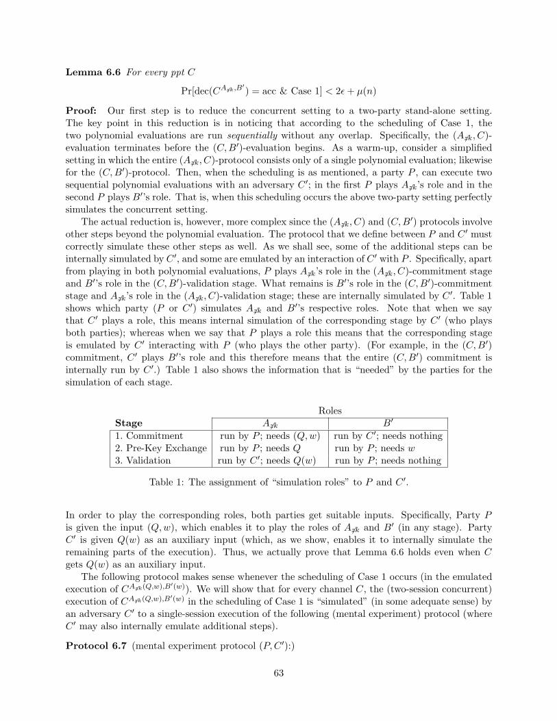
Lemma 6.6 For every ppt C

Pr[dec(CA6zk,B′) = acc & Case 1] < 2ε + µ(n)

Proof: Our first step is to reduce the concurrent setting to a two-party stand-alone setting.The key point in this reduction is in noticing that according to the scheduling of Case 1, thetwo polynomial evaluations are run sequentially without any overlap. Specifically, the (A6zk, C)-evaluation terminates before the (C, B′)-evaluation begins. As a warm-up, consider a simplifiedsetting in which the entire (A6zk, C)-protocol consists only of a single polynomial evaluation; likewisefor the (C, B′)-protocol. Then, when the scheduling is as mentioned, a party P , can execute twosequential polynomial evaluations with an adversary C ′; in the first P plays A6zk’s role and in thesecond P plays B′’s role. That is, when this scheduling occurs the above two-party setting perfectlysimulates the concurrent setting.

The actual reduction is, however, more complex since the (A6zk, C) and (C, B′) protocols involveother steps beyond the polynomial evaluation. The protocol that we define between P and C ′ mustcorrectly simulate these other steps as well. As we shall see, some of the additional steps can beinternally simulated by C ′, and some are emulated by an interaction of C ′ with P . Specifically, apartfrom playing in both polynomial evaluations, P plays A6zk’s role in the (A6zk, C)-commitment stageand B′’s role in the (C, B′)-validation stage. What remains is B′’s role in the (C,B′)-commitmentstage and A6zk’s role in the (A6zk, C)-validation stage; these are internally simulated by C ′. Table 1shows which party (P or C ′) simulates A6zk and B′’s respective roles. Note that when we saythat C ′ plays a role, this means internal simulation of the corresponding stage by C ′ (who playsboth parties); whereas when we say that P plays a role this means that the corresponding stageis emulated by C ′ interacting with P (who plays the other party). (For example, in the (C, B′)commitment, C ′ plays B′’s role and this therefore means that the entire (C,B′) commitment isinternally run by C ′.) Table 1 also shows the information that is “needed” by the parties for thesimulation of each stage.

RolesStage A6zk B′

1. Commitment run by P ; needs (Q,w) run by C ′; needs nothing2. Pre-Key Exchange run by P ; needs Q run by P ; needs w3. Validation run by C ′; needs Q(w) run by P ; needs nothing

Table 1: The assignment of “simulation roles” to P and C ′.

In order to play the corresponding roles, both parties get suitable inputs. Specifically, Party Pis given the input (Q,w), which enables it to play the roles of A6zk and B′ (in any stage). PartyC ′ is given Q(w) as an auxiliary input (which, as we show, enables it to internally simulate theremaining parts of the execution). Thus, we actually prove that Lemma 6.6 holds even when Cgets Q(w) as an auxiliary input.

The following protocol makes sense whenever the scheduling of Case 1 occurs (in the emulatedexecution of CA6zk(Q,w),B′(w)). We will show that for every channel C, the (two-session concurrent)execution of CA 6zk(Q,w),B′(w) in the scheduling of Case 1 is “simulated” (in some adequate sense) byan adversary C ′ to a single-session execution of the following (mental experiment) protocol (whereC ′ may also internally emulate additional steps).

Protocol 6.7 (mental experiment protocol (P,C ′):)

63

Inputs:

• P has (Q,w), where Q is a linear (non-constant) polynomial and w ∈ D.

• C ′ receives the string Q(w), where (Q,w) is the input of P .

Operation:

1. Emulation of Stage 1 of the (A6zk, C)-execution (commitment stage):

• P sends C ′ a non-malleable commitment to (Q,w).

2. Emulation of Stage 2 of the (A6zk, C)-execution (pre-key exchange):

• P sends C ′ a commitment c1 = Commit(Q) = C(Q, r1) for a random r1.

• P and C ′ invoke an augmented polynomial evaluation, where P inputs the polynomial Qand (c1, r1) and C ′ inputs c1 and some value wC (of its choice). Party C ′ then receivesthe output value Q(wC) (or ⊥ in the case of incorrect inputs).

3. Emulation of Stage 2 of the (C,B′)-execution (pre-key exchange):

• C ′ sends P a commitment c2 = C(QC , r2), for some polynomial QC and r2 (of itschoice).

• C ′ and P invoke another augmented polynomial evaluation (in the other direction),where C ′ inputs the polynomial QC and (c2, r2) and P inputs c2 and w. Party P receivesπ, which equals either QC(w) or ⊥, from the evaluation.

4. Emulation of Stage 3 of the (C,B′)-execution (validation stage):

• C ′ sends a string y to P , and P outputs accept if and only if y = f2n(π).

We say that C ′ succeeds if P outputs accept at the conclusion of the protocol execution. We nowshow that any C succeeding in having B′ accept in the concurrent protocol with the schedulingof Case 1, can be used by a party C ′ to succeed with the same probability in the above protocolwith P . We prove this by having C ′ simulate the concurrent execution of C with A6zk and B′,while interacting with P . We note that in this simulation, the values QC and wC referred to inProtocol 6.7 intuitively represent the values that C uses in its secure polynomial evaluations withA6zk and B′. However, this intuition can only be formalized once the polynomial evaluations arereplaced with ideal executions (because in the real model, we cannot say anything about how Cworks, whereas in the ideal model, explicit QC and wC values must actually be produced).

Claim 6.8 Let C be a ppt channel interacting with A6zk and B′. Then there exists a ppt party C ′

interacting with P in Protocol-(P, C ′) such that

PrQ,w[P (Q,w) accepts when interacting with C ′(Q(w))] = Pr[dec(CA6zk,B′) = acc & Case 1]

Recall that CA6zk,B′ is actually a shorthand for CA 6zk(Q,w),B′(w), where (Q,w) are random as in thel.h.s above.

Proof: The party C ′ incorporates C internally and perfectly simulates the concurrent setting withA6zk and B′ for C (i.e., CA6zk(Q,w),B′(w)). First notice that Step (4) of the (P, C ′) protocol constitutesthe full validation stage of the (C, B′)-protocol (recall that the validation stage for B′ consists onlyof checking that y = f2n(πB)). This means that the (P,C ′) protocol contains all stages of the(A6zk, C) and (C,B′) protocols, except for the first stage of the (C,B′)-protocol and the third stageof the (A6zk, C)-protocol. As mentioned above, these stages are internally simulated by C ′.

64

The C ′ simulation: We now describe how C ′ runs the simulation. Party C ′ invokes C andemulates the CA6zk(Q,w),B′(w) setting for it, while interacting with P . This involves separatelysimulating the (A6zk, C) and (C, B′) executions. This simulation is carried out as follows (recallthat C fully controls the scheduling):• The (A6zk, C) Execution:

1. Stages 1 and 2: All messages from these stages of the execution are passed between C andP (without any change). That is, C ′ forwards any messages sent from C (to A6zk) to P andlikewise, messages from P are forwarded to C.

2. Stage 3: C ′ internally emulates A6zk’s role here, and thus P is not involved at all. In thisstage C expects to receive the string y = f2n(Q(w)) and a MAC of the (A6zk, C) session-transcript keyed by k1(Q(w)). Party C ′ can determine and send these messages since ithas Q(w) as input, and can thus compute both the y-string and the MAC-key (and so theMAC value).

• The (C, B′) Execution:

1. Stage 1: C ′ internally emulates B′’s role here, and thus P is not involved at all. Recallthat B′’s role in this stage is as the receiver of a non-malleable commitment; therefore nosecret information is needed by C ′ to emulate this part (by using C).

2. Stages 2 and 3: When C sends the first message belonging to Stage 2 of the (C, B′)-execution, party C ′ acts as follows:

• Scheduling Violation Case: If this first message was sent before the completion ofStage 2 of the (A6zk, C) execution (i.e., the scheduling of Case 1 does not hold), then C ′

halts (the simulation fails).

• Scheduling Conforming Case: If this first message was sent after the completion ofStage 2 of the (A6zk, C) execution (i.e., the scheduling conforms with Case 1), then C ′

continues the simulation by forwarding this and all consequent messages belonging tothese stages to P (and returning messages from P to C).

This completes the simulation. Note that, when the simulation succeeds, C’s view is identical toa real execution with A6zk and B′. Recall that the (P,C)-protocol emulates Stages 1 and 2 of the(A6zk, C) protocol before Stages 2 and 3 of the (C, B′) protocol. Therefore, the simulation succeedsas long as C’s scheduling is such that Stage 2 of the (A6zk, C) execution is completed before Stage 2of the (C,B′) execution begins. However this is exactly the definition of the scheduling of Case 1.In other words, the simulation is successful if and only if the scheduling is according to Case 1.Now, if the simulation is successful, then P accepts with the same probability as B′ would have.On the other hand, if the simulation is not successful (i.e., Case 1 did not occur), then P neveraccepts. We conclude that the probability that P accepts is exactly equal to the probability thatthe scheduling is according to Case 1 and B′ accepts.

We note that since C ′ is given the value Q(w), it can also simulate this scenario for C when theaugmented definition of security is considered. (In the case that A6zk finishes first, its output key isalways a function of Q(w), and so the challenge session-key is either uniform or the same functionof Q(w). On the other hand, the case that B finishes first makes no difference because the challengesession-key is presented after B’s decision bit is determined, and here we bound the probabilitythat B’s decision bit equals accept.) The rest of the proof of this lemma therefore follows also forthe augmented definition.

It remains to bound the probability that P accepts in Protocol 6.7.

65

Claim 6.9 For every ppt party C ′ interacting with P in Protocol 6.7 it holds that

PrQ,w[P (Q,w) accepts when interacting with C ′(Q(w))] < 2ε + µ(n)

Proof: We analyze the probability that P accepts in the two-party protocol for P and C ′ definedabove. This is an ordinary two-party setting, and as such it can be analyzed by directly consideringthe security of the different modules.

We first modify the protocol so that in Step 1, party P sends a random commitment, insteadof a commitment to (Q,w). Due to the hiding property of the commitment, this can make at mosta negligible difference. (We stress that this replacement has no impact because this commitmentis not used anywhere in the rest of the protocol.40) Therefore, C ′ can internally emulate thiscommitment and this stage can be removed from the protocol. We thus remain with a protocolconsisting of the following stages:• (Emulation of Stage 2 of (A6zk, C)): P sends C ′ a commitment to Q and then P and C ′ execute

an augmented polynomial evaluation in which C ′ receives either Q(wC) for some wC (chosenby C ′), or ⊥. By the security of the polynomial evaluation, C ′ receives either Q(wC) or ⊥ andnothing else.

• (Emulation of Stage 2 of (C, B′)): C ′ sends P a commitment to some polynomial QC and thenC ′ and P execute an augmented polynomial evaluation in which P receives QC(w) or ⊥. Bythe security of the polynomial evaluation, C ′ receives nothing in this stage.

• (Emulation of Stage 3 of (C, B′)): C ′ sends a string y to P and P accepts if y = f2n(QC(w)).The intuition behind showing that P accepts with probability at most negligibly greater than 2ε isas follows: C ′ must send the “correct” y based solely on the value Q(wC) that it (possibly) receivedfrom the first evaluation and its auxiliary input Q(w). Now, if wC 6= w, then the only thing thatparty C ′ learns about w (from Q(w) and Q(wC)) is that it does not equal wC . This is due tothe “pairwise independence” property of the random polynomial Q. Therefore, C must guess thecorrect value for y from |D| − 1 possibilities (i.e., f2n(QC(w′)) for every w′ 6= wC). On the otherhand, the probability that wC = w is at most ε, because at the time that C ′ selects wC it knowsnothing about w (although it knows Q(w) for a random Q). A detailed analysis follows.

The above argument is based on the security of the polynomial evaluations. We therefore proceed byanalyzing the probability that P accepts in an ideal execution where the two polynomial evaluationsare replaced by ideal evaluations. We denote the ideal-model parties by P and C ′. By the sequentialcomposition theorem of multi-party computation [16], we have that the accepting probabilities ofP (in a real execution) and P (in an ideal execution) are at most negligibly different.

We now upper bound the probability that P accepts in an ideal execution. Party C ′ is givenQ(w) for auxiliary input and in the first polynomial evaluation C ′ inputs a value wC (of its choice).We differentiate between the case that wC = w and wC 6= w, and separately upper bound thefollowing probabilities:

1. Pr[P = acc & wC = w]

2. Pr[P = acc & wC 6= w]40This is due to the fact that the zero-knowledge protocol of Stage 3 has already been removed.

66

Bounding the probability that P = acc and wC = w: We actually show that Pr[wC = w] ≤ε + µ for some negligible function µ. The only message received by C ′ prior to its sending wC is an(ordinary) commitment to the polynomial Q. That is, C ′’s entire view at this point consists of itsauxiliary input Q(w) and Commit(Q). Due to the hiding property of the commitment, Commit(Q)can be replaced by Commit(02n) and this makes at most a negligible difference. We therefore removethe commitment and bound the probability that wC = w, where C ′ is only given Q(w). Since Qis a random linear polynomial, we have that for every w, the string Q(w) is uniformly distributed.That is, Q(w) reveals no information about w. Therefore, we have that Pr[wC = w] ≤ ε (withequality in case wC ∈ D). This implies that when C ′ is given a commitment to Q (rather than to02n), we have that Pr[wC = w] ≤ ε + µ(n). Therefore,

Pr[P = acc & wC = w] ≤ Pr[wC = w] ≤ ε + µ(n) (32)

Bounding the probability that P = acc and wC 6= w: We actually analyze the followingconditional probability: Pr[P = acc | wC 6= w]. Recall that C ′’s view (after the first polynomialevaluation) consists of its random tape, auxiliary input Q(w) and the following messages:

1. A commitment to a polynomial Q sent by P .

As before, the commitment to Q can be replaced with a commitment to 02n with at most anegligible difference. We therefore ignore this part of C ′’s view from now on.

2. An input–output pair (wC , Q(wC)) (or (wC ,⊥) in the case of incorrect inputs) from the firstpolynomial evaluation, where wC 6= w.

We are going to ignore the output case (wC ,⊥), because C ′ knows a-priori which of the twoinput/output cases will occur, and we may give it Q(wC) for free in the incorrect inputs case.

The continuation of the protocol involves C ′ selecting and inputting a polynomial QC into the secondpolynomial evaluation and sending a string y, where P accepts if and only if y = f2n(QC(w)). Re-stated, the probability that P accepts equals the probability that C ′, given its view (Q(w), wC , Q(wC)),generates a pair (QC , y) such that y = f2n(QC(w)).

Now, the polynomial Q is random and linear, and we are considering the case that wC 6= w.Therefore, by pairwise independence we have that Q(w) is almost uniformly distributed, even giventhe value of Q at wC . (Since Q cannot be a constant polynomial, Q(w) is only statistically closeto uniform; this is however enough.) This means that given C ′’s view, the password w is almostuniformly distributed in D − {wC}. Since both f2n and QC are 1–1 functions, we have that theprobability that C ′ generates a pair (QC , f2n(QC(w))) equals the probability that it guesses w,which equals 1

|D|−1 = ε1−ε . Replacing the commitment to 02n with a commitment to Q, we have

that for some negligible function µ,

Pr[P = acc | wC 6= w] ≤ ε

1− ε+ µ(n) (33)

Combining the bounds: Using Eq. (32) and Eq. (33), we conclude that in an ideal execution:

Pr[P = acc] = Pr[P = acc | wC = w] · Pr[wC = w] + Pr[P = acc | wC 6= w] · Pr[wC 6= w]

≤ 1 · Pr[wC = w] +ε

1− ε· (1− Pr[wC = w]) + µ(n)

Pr[wC = w] =ε

1− ε+

1− 2ε

1− ε· Pr[wC = w] + µ(n)

≤(

1 + (1− 2ε))· ε

1− ε+ µ(n) = 2ε + µ(n)

67

where the last inequality is due to Pr[wC = w] ≤ ε + µ. This implies that in a real execution, theprobability that P accepts is at most negligibly greater than 2ε. The claim follows.

Lemma 6.6 follows by combining Claims 6.8 and 6.9.

Lemma 6.1 follows by combining Corollary 6.5 and Lemma 6.6.

6.2 Proof of Lemma 4.7 (The Synchronized Case)

Lemma 6.10 (Lemma 4.7 – restated; Case 2 - Synchronized): Let C be a ppt channel and defineCase 2 to be a scheduling of the protocol by which C completes the polynomial evaluation with Aafter completing the non-malleable commitment with B. Then

Pr[B = acc & πA 6= πB & Case 2] < ε + µ(n)

Proof: The proof of this lemma relies on the non-malleability of the commitment sent in thecommitment stage of the protocol. As was explained in the proof sketch, in the case that πA 6= πB,the validation stage ensures that B only accepts if the non-malleable commitment he received wasto (Q′, w), where Q′ 6= Q and w is A and B’s shared password. (Recall that in the case that(Q′, w′) = (Q, w), party B rejects with overwhelming probability, unless πA = πB.)41 Furthermore,the probability that C succeeds in generating such a commitment (in which Q′ 6= Q and yet wis the second element) is at most negligibly greater than ε. We now formally prove both thesestatements.

In order to use the non-malleability property (of the commitment sent in Stage 1), we definethe following relation R. Recall that the non-malleable commitment value sent by A is (Q,w),and denote the value corresponding to the commitment received by B by (Q′, w′). Define R ⊂{0, 1}3n × {0, 1}3n such that

((Q,w), (Q′, w′)) ∈ R if and only if (Q′, w′) 6= (Q,w) and w′ = w. (34)

That is, C “succeeds” with respect to R (and thus B may accept) if C does not copy A’s commitment(or rather does not commit to the same pair) and yet the second element of the committed pair isthe correct password.

We consider the probability that B accepts in Case 2 and πA 6= πB in two complementarysubcases. In the first subcase, channel C succeeds with respect to the relation R and in the secondsubcase, C fails. We prove claims showing the following:

1. Success Case: Pr[B = acc & Case 2 & πA 6= πB & ((Q,w), (Q′, w′)) ∈ R] < ε + µ(n)

2. Fail Case: Pr[B = acc & Case 2 & πA 6= πB & ((Q, w), (Q′, w′)) 6∈ R] < µ(n)

The lemma follows by summing up B’s accepting probability in the above two subcases. We beginby upper bounding the success case. Specifically, we show that the probability that C succeeds ingenerating a correct (related) commitment is at most negligibly greater than ε.

Claim 6.11 (Success w.r.t R): Let C be a ppt channel and denote by (Q′, w′) the value committedto by C in the non-malleable commitment received by B (if the commitment is not valid, then(Q′, w′) is taken as some fixed value). Then

Pr[Case 2 & ((Q,w), (Q′, w′)) ∈ R] < ε + µ(n)41This is because the validation stage essentially enforces that πB = Q′(w′) (see Fact 6.14), and by the case

hypothesis Q′(w′) = Q(w) = πA.

68

Proof: The definition of non-malleability states that a commitment is non-malleable when run con-currently with another commitment only. Therefore, in a simpler scenario in which the (A,C) and(C,B) non-malleable commitments are run in isolation, we can directly apply the non-malleabilityproperty to the relation R that we have defined above. However, in our scenario, other parts of the(A,C) protocol can also be run concurrently to the (C, B) non-malleable commitment. Specifically,by the scheduling of Case 2, (part of) the (A,C) pre-key exchange may run concurrently to the(B,C) commitment (but Stage 3 of the (A, C) execution starts only after the (B, C) commitmentends). The crux of the proof is in showing that the (A,C) pre-key exchange can be simulated. Givensuch a simulation, we have a scenario in which the (A,C) and (C, B) non-malleable commitmentsare run in isolation, and thus non-malleability holds.

Recall that A’s input to the pre-key exchange stage depends only on the polynomial Q (and isindependent of the password w). Therefore, if C has Q, then it can perfectly emulate this stage byitself (this is true irrespective of the security of the modules making up the pre-key exchange stageof the protocol). Fortunately, even if C is explicitly given Q, the probability that C can generate acommitment to (Q′, w′) for which (Q′, w′) 6= (Q,w) and w′ = w is at most negligibly greater thanε (recall that C’s sole aim here is to generate such a commitment). Thus, we prove that for everyppt channel C given auxiliary input Q, it holds that

Pr[Case 2 & ((Q,w), (Q′, w′)) ∈ R] < ε + µ(n)

As we have described, C has Q and thus can perfectly emulate the (A,C) pre-key exchange. By thescheduling of Case 2, we have that the (C,B) commit stage concludes before the completion of the(A,C) pre-key exchange. Therefore, the probability that C succeeds with respect to R is the sameas when the (A,C) and (C, B) non-malleable commitments are run in isolation.42 We thereforeproceed by upper-bounding the probability that a ppt adversary C (given a commitment to (Q,w)and auxiliary input Q) successfully generates a commitment to (Q′, w′) where ((Q,w), (Q′, w′)) ∈ R.

Intuitively, A’s commitment to (Q,w) does not help C in generating a related commitment.Therefore, the probability of generating a commitment to (Q′, w) is the same as the probability ofguessing w. Formally, by the definition of non-malleability, for every C there exists a simulator Cwho generates a commitment to (Q′, w′) without seeing the commitment to (Q,w) such that

∣∣∣Pr[((Q, w), (Q′, w′)) ∈ R]− Pr[((Q, w), (Q′, w′)) ∈ R]∣∣∣ < µ(n)

Since w is uniformly distributed in D and C is given no information about w, the probability thatC generates a commitment to (Q′, w) is at most ε. Therefore, the probability that C generates acommitment to (Q′, w) where Q′ 6= Q, is less than ε + µ(n) as required.

We note that the above holds also for the augmented definition of security. This is because inCase 2, channel C concludes its non-malleable commitment before A terminates. Therefore, it mayreceive a session-key challenge only after (Q′, w′) are determined.

We now show that when C fails with respect to R, then B accepts with at most negligible probability.

Claim 6.12 (Failure w.r.t R): For every ppt channel C,

Pr[B = acc & πA 6= πB & ((Q,w), (Q′, w′)) 6∈ R] < µ(n)42Formally, an adversary attacking a non-malleable commitment protocol (and given Q as auxiliary input) can use

C in order to generate a related commitment with the same probability as C succeeds in our session-key protocolwhen the scheduling is according to Case 2.

69

Proof: In proving this claim, we rely solely on the fact that C “fails” with respect to the relationR, in order to show that B rejects. As described in the proof sketch, intuitively B rejects in thiscase because the validation stage enforces consistency between the non-malleable commitment, thepolynomial input by C into the polynomial evaluation and B’s output from the polynomial eval-uation. That is, with overwhelming probability, B rejects unless C inputs Q′ into the polynomialevaluation and B’s output from the evaluation equals Q′(w′). However, B’s input into the polyno-mial evaluation is w, and thus (by the correctness condition of secure protocols) B’s output mustequal Q′(w). Thus, with overwhelming probability B rejects unless Q′(w′) = Q′(w). As we willshow, this implies that πA = πB, in contradiction to the claim hypothesis. In the following fact, weformally show that with overwhelming probability, when B accepts, its output from the polynomialevaluation equals Q′(w) (recall that Q′ is the polynomial committed to by C in the non-malleablecommitment).

Fact 6.13 For every ppt channel C,

Pr[B = acc & πB 6= Q′(w)] < µ(n)

Proof: This fact is derived from the correctness condition of the secure polynomial evaluationand the soundness of the zero-knowledge proof. Loosely speaking, the correctness condition of asecure two-party protocol states that an adversary cannot cause the output of an honest party tosignificantly deviate from its output in an ideal execution (where the output is exactly accordingto the functionality definition). We stress that this has nothing to do with privacy and holds evenif the adversary knows the honest party’s input.

Now, let QC be the polynomial in the ordinary commitment sent by C to B before the polyno-mial evaluation. Then, by the definition of the augmented polynomial evaluation, B’s output πB

is either QC(w) (in the case of correct inputs) or ⊥ (in the case of incorrect inputs). Therefore, ina stand-alone two-party setting, we have that with overwhelming probability πB ∈ {QC(w),⊥}.

We now show that this also holds in our concurrent setting. As we have mentioned, the cor-rectness requirement holds even if the adversary knows the honest party’s input. That is, it holdseven if C knows w (and Q), in which case C can perfectly emulate the entire (A,C) execution,and we remain with a non-concurrent execution with B. The correctness condition thus holds andwe conclude that with overwhelming probability πB ∈ {QC(w),⊥}. However, since B accepts onlyif y = f2n(πB) and this never holds when πB = ⊥, we have πB = QC(w) (with overwhelmingprobability). Getting back to our original concurrent setting, we have:

Pr[B = acc & πB 6= QC(w)] < µ(n)

The proof is completed by noticing that the statement proved in the zero-knowledge proof implies(among other things) that QC = Q′. Thus, by the soundness of the zero-knowledge proof (whichalso holds in our setting), we conclude that

Pr[B = acc & πB 6= Q′(w)] < µ(n)

On the other hand, we now show that when B accepts, with overwhelming probability it holds thatπB = Q′(w′).

Fact 6.14 For every ppt channel C,

Pr[B = acc & πB 6= Q′(w′)] < µ(n)

70

Proof: In the first step of the validation stage, B receives a string y. The statement provedby C (in zero-knowledge) includes the condition y = f2n(Q′(w′)). Furthermore, by another checkmade by B, it rejects unless y = f2n(πB). Since f2n is a 1–1 function, we conclude that withoverwhelming probability, B rejects unless πB = Q′(w′).

We now use the above two facts to show that when ((Q,w), (Q′, w′)) 6∈ R, party B rejects withoverwhelming probability. There are two possible cases for which ((Q,w), (Q′, w′)) 6∈ R: either(Q′, w′) = (Q, w) or w′ 6= w.• Case (Q′, w′) = (Q,w): By Fact 6.13 (or equivalently by Fact 6.14), we have that with over-

whelming probability, B rejects unless πA = Q(w) = Q′(w′) = πB, in contradiction to thehypothesis that πA 6= πB.

• Case w′ 6= w: By Facts 6.13 and 6.14 that with overwhelming probability whenever B acceptsit holds that Q′(w′) = πB = Q′(w). However, Q′ is a non-constant linear polynomial and is thus1–1. This implies that w′ = w, in contradiction to the case hypothesis.

This completes the proof of Claim 6.12. We note that the above proof also holds for the augmenteddefinition of security. This can be seen by noticing that B rejects with overwhelming probabilityeven if C knows Q and w. Therefore, C can generate the session-key challenge itself.

Lemma 6.10 is obtained by combining Claims 6.11 and 6.12.

7 Simulating the Stand-Alone (A,C) Execution

In this section we show that C’s view of its execution with A can be simulated by a non-interactivemachine C ′′. That is,

Theorem 7.1 (Theorem 4.8 restated): For every ppt channel C ′ interacting with A only, thereexists a non-interactive machine C ′′, such that

{w, k2(Q(w)), output(C ′A(Q,w)(σ))

}n,D,σ

2ε≡ {w, Un, output(C ′′(σ))

}n,D,σ

where Q is a random non-constant linear polynomial, D ⊆ {0, 1}n is any ppt samplable dictionary,w ∈R D, and ε = 1

|D| .

Proof: As we described in the proof sketch, it is enough to prove that for every ppt channel C ′,{w, k2(Q(w)), output(C ′A(Q,w)(σ))

}2ε≡

{w,Un, output(C ′A(Q,w)(σ))

}

where w, w ∈R D are independently chosen passwords from D. This implies the theorem becauseC ′′ can simulate C ′’s view by choosing Q and w and invoking an execution of C ′A(Q,w)(σ). See theproof sketch for details on how C ′′ works.

Notice that the distributions {w,Un, output(C ′A(Q,w))} and {w, Un, output(C ′A(Q,w))} are equiv-alent. We therefore continue by showing that,

{w, k2(Q(w)), output(C ′A(Q,w))

}2ε≡

{w, Un, output(C ′A(Q,w))

}(35)

We begin by showing that the pair (w,Q(w)) is (1 − ε)-indistinguishable from (w, Un) at the endof the polynomial evaluation. For this aim, we consider a modified party A2 who halts at theconclusion of Stage 2 of the protocol (i.e., after the polynomial evaluation). Then, we show thatafter an execution of C with A2, the pair (w, Q(w)) is (1−ε)-indistinguishable from the pair (w, Un)with respect to C’s view. That is,

71

Lemma 7.2 For every ppt channel C ′ interacting with a party A2 who halts after the polynomialevaluation, {

w, Q(w), output(C ′A2(Q,w))}

ε≡{w, Un, output(C ′A2(Q,w))

}

where Q is a random non-constant linear polynomial, and w, w ∈R D.

Proof: First note that the non-malleable commitment sent by A2 in this setting plays no role in thecontinuation of the protocol (the commitment is referred to only in the validation stage, which A2

does not reach). Due to the hiding property of the commitment, if A2 commits to all-zeros insteadof to the pair (Q,w), this makes at most a negligible difference to C ′’s view. This enables us toremove the non-malleable commitment entirely, because C ′ can internally simulate receiving such acommitment. From here on, we consider the modified party A2 to be a party whose non-malleablecommitment is to zeros and who halts after the polynomial evaluation.

What remains is thus the (A2, C′) pre-key exchange, consisting of A2 sending Commit(Q) to C ′

followed by a single polynomial evaluation. Since the polynomial evaluation is secure, C can learnat most a single point of Q(·), but otherwise gains no other knowledge of the random polynomialQ (as with the non-malleable commitment, Commit(Q) reveals nothing of Q). As described in theproof sketch, this implies that C can distinguish Q(w) from Un with probability at most negligiblygreater than ε (where the ε advantage comes from the case that w turns out to equal the inputfed by C ′ into the polynomial evaluation). We now formally show how the limitation on C ′’sdistinguishing capability is derived from the security of the polynomial evaluation.

The security of the polynomial evaluation states that C ′ can learn no more in a real executionthan in an ideal scenario where the polynomial evaluation is replaced by an ideal module computedby a trusted third party. We stress that the other messages sent by the parties in the protocol,including the commitment to Q, remain unmodified in this (partially) ideal execution. Denote

the ideal model parties by A2 and C ′ and an ideal execution by C ′A2(Q,w)(in this execution, C ′

is adversarial). By the definition of secure two-party computation, for every real adversary C ′

interacting with A2, there exists an ideal adversary C ′ interacting with A2 such that the outputdistributions of C ′ and C ′ are computationally indistinguishable. However, by the definition ofsecure computation, the above output distributions should be indistinguishable also when givenparties’ respective inputs, and specifically A’s input (Q,w). That is,

{(Q,w), output(C ′A2(Q,w))

}c≡

{(Q,w), output(C ′A2(Q,w)

)}

In particular it follows that

{w, Q(w), output(C ′A2(Q,w))

}c≡

{w, Q(w), output(C ′A2(Q,w)

)}

(36)

{w, Un, output(C ′A2(Q,w))

}c≡

{w, Un, output(C ′A2(Q,w)

)}

(37)

Thus, it suffices to show that for every ppt party C ′ interacting with A2 in an ideal execution, itholds that {

w, Q(w), output(C ′A2(Q,w))}

ε≡{

w, Un, output(C ′A2(Q,w))}

(38)

We therefore consider an ideal execution of the pre-key exchange consisting of A2 sending C ′ acommitment to Q followed by an ideal augmented polynomial evaluation. The view of C ′ in such

72

an execution consists only of a commitment to Q and the result of the polynomial evaluation. (Theexact definition of the augmented polynomial evaluation can be found in Section 3.)

Notice that the distributions {w, Un, output(C ′A2(Q,w))} and {w,Un, output(C ′A2(Q,w)

)} areequivalent. This is because A2 uses w nowhere in the execution (recall that the non-malleablecommitment sent by A2 is to all-zeros). Therefore, we should actually show that,

{w, Q(w), output(C ′A2(Q,w)

)}

ε≡{

w, Un, output(C ′A2(Q,w))}

(39)

Assume for now that the execution of the polynomial evaluation is such that C ′ always receivesQ(wC) for some wC input by it into the evaluation (and not ⊥ as in the case of incorrect in-puts). Then, C ′’s view is exactly (r,Commit(Q), Q(wC)), where r is the string of its randomcoin tosses and wC is determined by C ′ based on r and Commit(Q). For the sake of clar-ity, we augment the view by wC itself (i.e., we write C ′’s view as (r,Commit(Q), wC , Q(wC))).Assuming without loss of generality that C ′ always outputs its entire view, we conclude thatour aim is to show that {w, Q(w), (r,Commit(Q), wC , Q(wC))} is (1 − ε)-indistinguishable from{w,Un, (r,Commit(Q), wC , Q(wC))}. We now show that if wC 6= w, then the above two tuples arecomputationally indistinguishable. That is, we show that

{w,Q(w), (r,Commit(Q), wC , Q(wC)) | wC 6= w}c≡ {w,Un, (r,Commit(Q), wC , Q(wC)) | wC 6= w} (40)

where Q is a random non-constant linear polynomial. First, by the hiding property of the com-mitment scheme, we can replace the commitment to Q in the above distributions with a com-mitment to 02n. (If this makes a non-negligible difference, then C ′ can be used to distinguisha commitment to Q from a commitment to 02n. We remark that this argument actually onlyholds if the probability that wC 6= w is non-negligible. However, this follows from the fact thatw ∈R D appears nowhere in the C ′A2(Q,w)

execution (recall that the non-malleable commitmenthas been replaced with a commitment to zeros). Therefore, wC = w with probability at most ε.)Next, having replaced the commitment to Q by a commitment to 02n, notice that the follow-ing distributions are statistically close: {w, Q(w), (r,Commit(02n), wC , Q(wC)) | wC 6= w} and{w,Un, (r,Commit(02n), wC , Q(wC)) | wC 6= w}.43 Then, by returning the commitment to Q inplace of the commitment to 02n, we obtain Eq. (40).

As we have mentioned, the password w ∈R D does not appear anywhere in the C ′A2(Q,w)

execution. Therefore, Pr[wC = w] ≤ ε (with equality when wC is chosen from D). Therefore, byseparately considering the case that wC 6= w (where the distributions cannot be distinguished) andthe case that wC = w (which occurs with probability at most ε), Eq. (39) follows.

This completes the analysis of the simplified case in which the output from the polynomialevaluation is always Q(wC) for some wC (and never ⊥). However, C ′ may cause the result of theevaluation to be ⊥ and we must show that this cannot help it. Intuitively, if C ′ were to receive ⊥then it would learn nothing about Q and this would thus be a “bad” strategy. Nevertheless, it mustbe shown that C ′ cannot learn anything by the mere fact that it received ⊥ and not Q(wC). The

43If Q was randomly chosen from all linear polynomials (rather than only from those that are non-constant),then due to pairwise independence the distributions would be identical. However, because Q cannot be constant,wC 6= w implies that Q(wC) 6= Q(w) always. On the other hand, Q(wC) = Un with probability 2−n. Therefore, withprobability 2−n the two distributions can be distinguished by seeing if the last two elements are equal or not. Thisis the only difference between the distributions and they are therefore statistically close.

73

reason that C ′ indeed learns nothing from the latter event is because it can determine it a-priori(i.e., the output is ⊥ if and only if C ′ does not supply the commitment explicitly sent to it in theprevious step by the honest A (which will always input the corresponding decommit information)).This completes the proof of Lemma 7.2.

We now continue by showing that Lemma 7.2 implies Eq. (35) (and thus the current theorem);that is, {

w, Q(w), output(C ′A2(Q,w))}

ε≡{w, Un, output(C ′A2(Q,w))

}

implies that {w, k2(Q(w)), output(C ′A(Q,w))

}2ε≡

{w, Un, output(C ′A(Q,w))

}

Notice that in the second equation, C ′ executes a complete execution of the protocol with A,rather than a truncated execution with A2. Therefore, the additional messages sent by A in thevalidation stage must be taken into account. Recall that in the validation stage A sends the stringy = f2n(Q(w)), proves a statement in zero-knowledge and sends a MAC (keyed by k1(Q(w))) ofthe entire message transcript. In order to simplify the proof, we assume that A sends the MAC-keyk1(Q(w)) itself during the validation stage. Given the MAC-key (i.e., k1(Q(w))), the channel C ′

can always compute the MAC value by itself. Therefore, this only gives C ′ more information. Westart by ignoring the zero-knowledge proof (which, as we show below, is easily justified in thiscontext).

The proof is based on the fact that since G(s) = (f2n(s), k1(s), k2(s)) is a pseudorandom gen-erator, the output key k2(Q(w)) is (1−O(ε))-pseudorandom, even given f2n(Q(w)) and k1(Q(w)).This must be justified, since in our case the generator is seeded by Q(w) that is only (1 − ε)-pseudorandom, whereas a generator is usually seeded by a truly random string. In the followingclaim we show that if, given some information, the string Q(w) is (1 − ε)-pseudorandom (as pre-viously shown), then given the same information along with f2n(Q(w)) and k1(Q(w)), the stringk2(Q(w)) is (1 − 2ε)-pseudorandom. (By “given” we mean that a ppt distinguishing machine isgiven these strings, along with the challenge string which is either k2(Q(w)) or Un.) Applied to theanalysis of our protocol, this means that even after A sends the string f2n(Q(w)) and the MAC inthe validation stage, the output session-key k2(Q(w)) is (1− 2ε)-pseudorandom with respect to theview of C ′.

Claim 7.3 Let I(·) be a random process, and assume that {w, Q(w), I(Q,w)} is (1−ε)-indistinguishablefrom {w, Un, I(Q,w)}. Then {w, k2(Q(w)), I(Q,w), f2n(Q(w)), k1(Q(w))} is (1−2ε)-indistinguishablefrom {w, Un, I(Q,w), f2n(Q(w)), k1(Q(w))}.

Indeed, the claim will be applied with I(Q,w) = output(C ′A2(Q,w)).

Proof: We prove the claim in three steps:

1. {w, I(Q,w), f2n(Q(w)), k1(Q(w)), k2(Q(w))} ε≡ {w, I(Q,w), f2n(Un), k1(Un), k2(Un)}.This is due to the hypothesis {w, I(Q,w), Q(w)} ε≡ {w, I(Q, w), Un}.

2. {w, I(Q,w), f2n(Un), k1(Un), k2(Un)} c≡ {w, I(Q,w), f2n(U (1)n ), k1(U

(1)n ), U (2)

n }, where U(1)n and

U(2)n are two independent uniform distributions.

This is derived directly from the fact that (f2n(Un), k1(Un), k2(Un)) is pseudorandom.

74

3. {w, I(Q,w), f2n(U (1)n ), k1(U

(1)n ), U (2)

n } ε≡ {w, I(Q,w), f2n(Q(w)), k1(Q(w)), U (2)n }

This is because the hypothesis implies that {I(Q,w), Un} ε≡ {I(Q, w), Q(w)}.Combining the above, we have that

{w, I(Q,w), f2n(Q(w)), k1(Q(w)), k2(Q(w))} 2ε≡ {w, I(Q,w), f2n(Q(w)), k1(Q(w)), Un}and this completes the proof of the claim.

Combining Lemma 7.2 and Claim 7.3, we now establish Eq. (35). We use the following facts:

1. In Stage 3, A sends the string y = f2n(Q(w)), proves a statement in zero-knowledge andsends the MAC-key k1(Q(w)) (recall that we assume that A sends the MAC-key instead ofthe MAC-value).

2. C ′ can simulate the zero-knowledge proof given by A in Stage 3, because here we are consider-ing a stand-alone execution between A and C. Thus, the view of C ′ from the entire interactionwith A can be generated out of its view of the first two stages (i.e., output(C ′A2(Q,w))), thestring y = f2n(Q(w)) and the MAC-key k1(Q(w)).

Using I(Q,w) def= output(C ′A2(Q,w)), Lemma 7.2 asserts that the corresponding hypothesis ofClaim 7.3 holds. The corresponding conclusion (of Claim 7.3) implies that Eq. (35) holds (be-cause output(C ′A(Q,w)) is easily computed from output(C ′A2(Q,w)), y = f2n(Q(w)) and k1(Q(w))).The theorem follows.

As we have mentioned in the proof sketch, the above proof remains unchanged when proving thesecurity of Protocol 3.2 with respect to the augmented definition of security (Def. 2.5). This isbecause in a stand-alone execution between A and C ′, the channel C ′ is given the session-keychallenge only after the entire execution has been completed. Therefore, the session-key challengecan be generated from the input/output distribution as a post-processing step.

8 Simulating the (C, B) Execution

In this section we show how the entire (C,B) execution can be simulated. The simulation is suchthat the joint distribution of C’s view in the simulation along with the password and session key isat most (1 − 5ε)-indistinguishable from the joint distribution of its view in a real execution alongwith the password and session-key.

Theorem 8.1 (Theorem 4.9 restated – simulating the (C, B) execution): For every ppt channelC interacting with A and B, there exists a ppt channel C ′ interacting only with A, such that

{w, k2(Q(w)), output(C ′A(Q,w)(σ))

}n,D,σ

5ε≡{w, k2(Q(w)), output(CA(Q,w),B(w)(σ))

}n,D,σ

where Q is a random non-constant linear polynomial, D ⊆ {0, 1}n is any ppt samplable dictionary,w ∈R D, and ε = 1

|D| .

Proof: As we have described in the proof sketch, this lemma is proved in two stages. First, inLemma 8.2, we show that when C interacts with A and a modified party B6dec who does not outputany accept/reject bit, then the (C, B6dec) execution can be simulated. Next, in Lemma 8.3, we showthat B’s accept/reject bit can also be simulated. Combining these two lemmas together, we havethat the entire (C,B) execution can be simulated.

75

8.1 Simulating the (C, B 6dec) Execution

Lemma 8.2 (Lemma 4.10 restated): Let C be a ppt channel interacting with A and a modifiedparty B 6dec who does not output an accept/reject bit. Then, there exists a ppt channel C ′ interactingwith A only, such that

{w, k2(Q(w)), output(C ′A(Q,w))

}c≡

{w, k2(Q(w)), output(CA(Q,w),B 6dec(w))

}

Proof: Intuitively, B6dec’s role can be simulated without any knowledge of w. Loosely speaking,this is because B 6dec only uses w in the (C, B6dec) polynomial evaluation, and in this evaluation Creceives no output. Formally, this is shown by proving that if B 6dec were to input an arbitrary,fixed w′ ∈R D (into the polynomial evaluation), instead of w, then C would not be able to tell thedifference. That is, for every ppt channel C,

{w, k2(Q(w)), output(CA(Q,w),B 6dec(w))

}c≡

{w, k2(Q(w)), output(CA(Q,w),B 6dec(w

′))}

(41)

(Observe that in the second distribution, B6dec’s input is w′.) We prove Eq. (41) even when C isgiven Q and w as auxiliary input. Now, since Q and w constitute all of A’s input, the channelC(Q,w) can perfectly simulate the entire (A,C) execution. That is, for every ppt channel C thereexists a ppt channel C such that the following two equations hold:

{w, k2(Q(w)), output(CB 6dec(w)(Q,w))} ≡ {w, k2(Q(w)), output(CA(Q,w),B6dec(w)(Q,w))}{w, k2(Q(w)), output(CB6dec(w

′)(Q,w))} ≡ {w, k2(Q(w)), output(CA(Q,w),B6dec(w′)(Q,w))}

It thus remains to show that{w, k2(Q(w)), output(CB 6dec(w)(Q,w))

}c≡

{w, k2(Q(w)), output(CB 6dec(w

′)(Q,w))}

(42)

The latter is derived from the security of the polynomial evaluation. Intuitively, C obtains nooutput from the polynomial evaluation, whereas the polynomial evaluation is the only part of theentire protocol in which B6dec uses his input (of w or w′). Formally, we may consider a ppt C ′

that emulates the entire (C, B6dec) execution except for the polynomial evaluation that it actuallyperforms with B′ that uses input w or w′. That is, B′ is merely playing receiver in the polynomialevaluation protocol, whereas C ′ is some (fancy) adversary for that protocol. Still, the security ofthe latter protocol (as stand-alone) implies that C ′ cannot distinguish the case that B′ has input wfrom the case that it has input w′ (because the ideal-model adversary cannot do so). We concludethat C can distinguish the cases that B6dec has input w or w′ with at most negligible probability.Eq. (42) follows, and thus so does Eq. (41).

We are now ready to show how C ′ works (recall that C ′ interacts with A only and its aimis to emulate an execution of C with A and B6dec). Machine C ′ begins by selecting an arbitraryw′ ∈ D. Then, C ′ perfectly emulates an execution of CA(Q,w),B 6dec(w

′) by playing B6dec’s role inthe (C, B 6dec) execution (C ′ can play B6dec(w′)’s role because w′ is known to it), and relaying allmessages belonging to the (A,C) execution (i.e., passing each message sent by A to C, and eachmessage sent by C to A). Finally, C ′ outputs whatever C does. By the definition of C ′, we have

{w, k2(Q(w)), output(CA(Q,w),B 6dec(w

′))}≡

{w, k2(Q(w)), output(C ′A(Q,w))

}(43)

The lemma follows from Equations (41) and (43).

76

8.2 Simulating B’s Accept/Reject Decision Bit

Lemma 8.3 (Lemma 4.11 restated): Let B 6dec be a modified party that does not output an ac-cept/reject bit. Then, for every ppt channel C interacting with A and B, there exists a ppt channelC interacting with A and B6dec, such that

{w, k2(Q(w)), output(CA(Q,w),B 6dec(w))

}5ε≡

{w, k2(Q(w)), output(CA(Q,w),B(w))

}

Proof: We prove this lemma by showing how the accept/reject bit of B can be predicted by C.Specifically, we show that the MAC sent in the validation stage is such that if C was not reliable,then B rejects with probability 1−5ε. This enables C to “predict” B’s output-bit based on whetheror not C was reliable. We thus start by proving the security of the MAC when keyed by k1(πA)(recall that πA

def= Q(w)). As we have mentioned in the proof sketch, we need to show that theMAC is secure only before B outputs its accept/reject bit. Thus, we consider a scenario in whichC interacts with A and the modified party B6dec. In the following claim, we formally state thesecurity of the MAC. (Recall that for simplicity, we consider an implementation of a MAC by apseudorandom function. However, our proof can be extended to any secure implementation of aMAC.)

Claim 8.4 (Claim 4.12 restated): Let C be an arbitrary ppt channel interacting with A and amodified party B6dec as in Lemma 8.3, and let tA and tB denote the transcripts from the (A,C)and (C,B 6dec) executions, respectively. Then, if tA 6= tB, it holds that the value MACk1(πA)(tB) is(1 − 2ε)-pseudorandom with respect to C’s view. That is, for every probabilistic polynomial-timedistinguisher D, every dictionary D ⊆ {0, 1}n, every auxiliary-input σ and all sufficiently large n’s

∣∣∣Pr[D(MACk1(πA)(tB), CA(Q,w),B 6dec(w)) = 1 & tA 6= tB]

−Pr[D(Un, CA(Q,w),B 6dec(w)) = 1 & tA 6= tB]∣∣∣ < 2ε + µ(n)

Proof: We prove this claim by first showing that the MAC-key k1(πA) is (1− 2ε)-pseudorandombefore A sends the MAC in the validation stage. Formally, consider a modified party A6mac who isexactly the same as A excepts that it does not send the MAC message. Then, we show that forevery ppt C, {

k1(Q(w)), CA6mac(Q,w),B 6dec(w)}

2ε≡{Un, CA6mac(Q,w),B 6dec(w)

}(44)

where Q is a random non-constant linear polynomial and w ∈R D. First, we claim that for everyppt channel C interacting with A6mac and B6dec, there exists a ppt channel C ′ interacting only withA6mac, such that {

k1(Q(w)), C ′A6mac(Q,w)}

c≡{k1(Q(w)), CA6mac(Q,w),B 6dec(w)

}

and {Un, C ′A6mac(Q,w)

}c≡

{Un, CA6mac(Q,w),B 6dec(w)

}

The above two equations can be shown in the same way as Lemma 8.2 above. Therefore, in order toobtain Eq. (44), it is enough to show that for every ppt channel C ′ interacting only with A6mac(Q,w)

{k1(Q(w)), C ′A6mac(Q,w)

}2ε≡

{Un, C ′A6mac(Q,w)

}

77

Now, by Lemma 7.2, we have that after the conclusion of the polynomial evaluation between A6mac

and C ′, it holds that Q(w) is (1−ε)-pseudorandom to C ′. We claim that this implies that k1(Q(w))is (1 − 2ε)-pseudorandom to C ′ at the conclusion of the complete protocol between A6mac and C.This can be shown using an almost identical proof as in Claim 7.3. (We note that here we arein a standard stand-alone setting, and so the zero-knowledge proof can be simulated, and revealsnothing about k1(Q(w)).) This completes the proof of Eq. (44).

We have so far established that the MAC-key k1(Q(w)) used by A is (1 − 2ε)-pseudorandomwith respect to C’s view. It thus remains to show that using a (1− 2ε)-pseudorandom string as akey to a pseudorandom function (for the MAC) yields a (1−2ε)-pseudorandom function. This thenimplies that when tA 6= tB, the value MACk1(πA)(tB) is (1− 2ε)-pseudorandom with respect to C’sview. (Recall that A sends MACk1(πA)(tA) in the protocol execution and thus this value itself isnot (1 − 2ε)-pseudorandom. However, since the MAC used is a (1 − 2ε)-pseudorandom function,the claim holds for any t that C produces, including tB that is part of its view.) In the followingclaim, we prove that MACk1(πA)(·) is a (1−2ε)-pseudorandom function. As in Claim 7.3, we modelany information C may have learned about Q and w during the protocol with A6mac by a randomprocess I(·) (i.e., I(Q,w) denotes output(CA6mac(Q,w))).

Claim 8.5 Assume that {k1(Q(w)), I(Q,w)} is (1−2ε)-indistinguishable from {Un, I(Q,w)}. Fur-thermore, let fr(·) be a pseudorandom function when r is uniformly distributed. Then, givenI(Q,w), the function fk1(Q(w))(·) is (1− 2ε)-pseudorandom.

Proof: The proof is based on the idea that a string distinguisher that needs to distinguish k1(Q(w))from Un can simulate oracle queries to fk1(Q(w))(·) or fUn(·) depending on its input. Since we knowthat fUn(·) is indistinguishable from a random function (by the claim hypothesis), distinguishingfk1(Q(w))(·) from a random function essentially means distinguishing k1(Q(w)) from Un. Detailsfollow.

Let D be a ppt oracle machine that receives the output of the random process I(Q,w) as wellas oracle access to either fk1(Q(w)) or a random function f . Then,

∣∣∣Pr[Dfk1(Q(w))(I(Q,w), 1n) = 1]− Pr[Df (I(Q,w), 1n) = 1]∣∣∣

≤∣∣∣Pr[Dfk1(Q(w))(I(Q,w), 1n) = 1]− Pr[DfUn (I(Q,w), 1n) = 1]

∣∣∣ (45)

+∣∣∣Pr[DfUn (I(Q,w), 1n) = 1]− Pr[Df (I(Q,w), 1n) = 1]

∣∣∣ (46)

Eq. (46) is negligible by the definition of a pseudorandom function. On the other hand, Eq. (45) isbounded above by 2ε + µ(n), because otherwise a ppt machine D′ that, given I(Q, w) and tryingto distinguish k1(Q(w)) from Un, can invoke D on input (I(Q,w), 1n) and answer all oracle queriesby using fx, where x denotes its input string (which is either k1(Q(w)) or Un).

This completes the proof of Claim 8.4.

We are now ready to show how C works. Channel C runs the protocol (with A and B6dec) by passingall messages, unmodified, via C. Furthermore, C checks whether or not C was reliable during theexecution. Recall that C is reliable if the (A, C) and (C, B) executions are run in a synchronizedmanner, and C does not modify any of the messages sent by A or B. This is a syntactic feature,which is easily checked by C (since it views the entire interaction). If C was reliable then C outputsaccept for B, otherwise it outputs reject for B. This completes the simulation of C’s interactionwith A and B. Let χC denote the simulated accept/reject bit output by C.

78

Now, when C predicts B’s output bit correctly, we have that C’s view in this simulation isidentical to a real execution with A and B. This means that the difference in the experimentsreferred to in the lemma’s conclusion equals the probability that C’s prediction is wrong (i.e., theprobability that decB = acc and χC = rej or vice versa). Noticing that χC = acc if and only if Cis reliable, we have that for every distinguisher D,

∣∣∣PrQ,w

[D

(w, k2(Q(w)), CA(Q,w),B 6dec(w)

)= 1

]− PrQ,w

[D

(w, k2(Q(w)), CA(Q,w),B(w)

)= 1

]∣∣∣≤ Pr[decB = acc & reliableC = false] + Pr[decB = rej & reliableC = true]

First, notice that when C is reliable, B always accepts. That is, Pr[decB = rej & reliableC = true]equals zero. We now show that Pr[decB = acc & reliableC = false] is at most negligibly more than5ε, and this completes the proof of Lemma 8.3.

Proposition 8.6 (Proposition 4.13 – restated): For every ppt channel C,

Pr[decB = acc & reliableC = false] < 5ε + µ(n)

Proof: The proof of this proposition is based on the security of the MAC sent in the validationstage. Intuitively, sending a MAC on the entire session transcript ensures that if any messageswere modified (as in the case of an unreliable C), then this will be noticed by B. However, inour protocol, A and B may have different MAC-keys (in which case nothing can be said aboutdetecting C’s malicious behavior). Fortunately, the key-match property ensures that this happens(undetectably by B) with probability at most 3ε.

The security of the MAC, shown above in Claim 8.4 states the following. Let tA and tB be Aand B’s respective message transcripts. Then if tA 6= tB, the string MACk1(πA)(tB) is (1 − 2ε)-pseudorandom with respect to C’s view. By the definition of reliability, if C is not reliable thenindeed tA 6= tB and so MACk1(πA)(tB) is (1− 2ε)-pseudorandom with respect to C’s view.

Now, party B’s protocol definition is such that he rejects unless the last message he receivesequals MACk1(πB)(tB), where k1(πB) is the MAC-key used by B. We stress that the key used by Bfor the MAC is k1(πB), whereas Claim 8.4 refers to a MAC keyed by k1(πA). However, if πA = πB

then k1(πA) = k1(πB). Therefore, if πA = πB then the claim holds and the probability that Cgenerates the correct MAC-value is at most negligibly greater than 2ε. That is,

Pr[B = acc & reliableC = false & πA = πB] < 2ε + µ(n)

On the other hand, if πA 6= πB then irrespective of the MAC, the probability that B accepts is atmost negligibly more than 3ε. This is due to the key-match property proven in Theorem 4.5. Weconclude that

Pr[decB = acc & reliableC = false]= Pr[decB = acc & reliableC = false & πA 6= πB]

+Pr[decB = acc & reliableC = false & πA = πB]< 3ε + 2ε + µ(n)

and the proposition follows.

As stated above, this completes the proof of Lemma 8.3.

79

8.3 Conclusion

Theorem 8.1 is obtained by combining Lemmas 8.2 and 8.3.

We note that when considering the augmented definition of security (Def. 2.5), the proof ofLemma 8.2 remains unchanged. This is because Eq. (41) (and thus the lemma) holds even inthe case that C is given Q and w and can generate the session-key challenge itself. On the otherhand, there are some minor differences in the proof of Lemma 8.3. In particular, one must justifythe correctness of Claim 8.4 even when C may also be given k2(Q(w)). That is, we must showthat the MAC-key k1(Q(w)) remains (1 − 2ε)-pseudorandom to C, even if it is given the session-key k2(Q(w)) as well. However, this is derived from the property of the pseudorandom generatorG(s) = (k1(s), k2(s), f2n(s)). The actual proof of this is very similar to that of Claim 7.3. Wemust also define how the challenge session-key is generated when B is replaced with B6dec. As wedescribed in the proof sketch, we define the challenge session-key in the case that B6dec concludesfirst to always equal ⊥. Then, we rely on the fact that if B6dec concludes first, this implies thatC was not reliable, and so B would reject (except with probability 5ε). Therefore, having thesession-key challenge equal ⊥ in this case makes no difference (modulo a 5ε difference). The restof the proof remains almost the same.

Acknowledgements

We would like to thank Moni Naor for suggesting this problem to us and for his valuable input in theinitial stages of our research. We are also grateful to Alon Rosen for much discussion and feedbackthroughout the development of this work. We also thank Jonathan Katz for helpful discussions,and Ran Canetti, Shai Halevi and Tal Rabin for discussion that led to a significant simplificationof the protocol. Finally, we thank the anonymous referees for their hard work and many helpfulcomments.

References

[1] B. Barak. Constant-Round Coin-Tossing With a Man in the Middle or Realizing theShared Random String Model. In the 43rd IEEE Symposium on the Foundations ofComputer Science, pages 345–355, 2002.

[2] D. Beaver. Secure Multi-party Protocols and Zero-Knowledge Proof Systems Toleratinga Fault Minority. Journal of Cryptology, 4(2):75–122, 1991.

[3] M. Bellare, R. Canetti and H. Krawczyk. Modular Approach to the Design and Analysisof Authentication and Key Exchange Protocols. In the 30th ACM Symposium on theTheory of Computing, pages 419–428, 1998.

[4] M. Bellare, D. Pointcheval and P. Rogaway. Authenticated Key Exchange Secure AgainstDictionary Attacks. In EUROCRYPT’00, Springer-Verlag (LNCS 1807), pages 139–155,2000.

[5] M. Bellare and P. Rogaway. Random Oracles are Practical: A Paradigm for Designing Ef-ficient Protocols. In the 1st ACM Conference on Computer and Communications Security,pages 62–73, 1993.

80

[6] M. Bellare and P. Rogaway. Entity Authentication and Key Distribution. In CRYPTO’93,Springer-Verlag (LNCS 773), pages 232–249, 1994.

[7] M. Bellare and P. Rogaway. Provably Secure Session Key Distribution: The Three PartyCase. In the 27th ACM Symposium on the Theory of Computing, pages 57–66, 1995.

[8] M. Bellare and M. Yung. Certifying Permutations: Non-Interactive Zero-Knowledge Basedon Any Trapdoor Permutation. In Journal of Cryptology, 9(3):149–166, 1996.

[9] S. M. Bellovin and M. Merritt. Encrypted key exchange: Password-based protocols secureagainst dictionary attacks. In the ACM/IEEE Symposium on Research in Security andPrivacy, pages 72–84, 1992.

[10] S.M. Bellovin and M. Merritt. Augmented encrypted key exchange: A password-basedprotocol secure against dictionary attacks and password file compromise. In the 1st ACMConference on Computer and Communication Security, pages 244–250, 1993.

[11] M. Blum. Coin Flipping by Phone. IEEE Spring COMPCOM, pages 133–137, February1982.

[12] M. Blum and S. Goldwasser. An Efficient Probabilistic Public-Key Encryption Schemewhich hides all partial information. In CRYPTO’84, Springer-Verlag (LNCS 196), pages289–302.

[13] M. Blum and S. Micali. How to Generate Cryptographically Strong Sequences of Pseudo-Random Bits. SIAM Journal of Computation, 13(4):850–864, 1984.

[14] M. Boyarsky. Public-key Cryptography and Password Protocols: The Multi-User Case.In the 6th ACM Conference on Computer and Communication Security, 1999.

[15] V. Boyko, P. MacKenzie and S. Patel. Provably Secure Password-Authenticated KeyExchange Using Diffie-Hellman. In EUROCRYPT’00, Springer-Verlag (LNCS 1807), pages156–171, 2000.

[16] R. Canetti. Security and Composition of Multi-party Cryptographic Protocols. Journalof Cryptology, 13(1):143–202, 2000.

[17] R. Canetti. Universally Composable Security: A New Paradigm for Cryptographic Pro-tocols. In the 42nd IEEE Symposium on the Foundations of Computer Science, pages136–145, 2001.

[18] R. Canetti and H. Krawczyk. Analysis of Key-Exchange Protocols and Their Use forBuilding Secure Channels. In EUROCRYPT’01, Springer-Verlag (LNCS 2045), pages453–474, 2001.

[19] R. Canetti, O. Goldreich, and S. Halevi. The Random Oracle Methodology, Revisited. Inthe 30th ACM Symposium on the Theory of Computing, pages 209–218, 1998.

[20] G. Di Crescenzo, Y. Ishai and R. Ostrovsky. Non-Interactive and Non-Malleable Commit-ment. In the 30th ACM Symposium on the Theory of Computing, pages 141-150, 1998.

[21] W. Diffie, and M.E. Hellman. New Directions in Cryptography. IEEE Transactions onInformation Theory, IT-22, pages 644–654, 1976

81

[22] W. Diffie, P.C. Van Oorschot and M.J. Wiener. Authentication and Authenticated KeyExchanges. Designs Codes and Cryptography, 2(2):107–125, 1992.

[23] D. Dolev, C. Dwork, and M. Naor. Non-Malleable Cryptography. SIAM Journal onComputing, 30(2):391–437, 2000.

[24] U. Feige and A. Shamir. Witness Indistinguishability and Witness Hiding Protocols. Inthe 22nd ACM Symposium on the Theory of Computing, pages 416–426, 1990.

[25] M. Fischlin and R. Fischlin. Efficient Non-malleable Commitment Schemes. InCRYPTO’00, Springer-Verlag (LNCS 1880), pages 413–431.

[26] Y. Gertner, S. Kannan, T. Malkin, O. Reingold and M. Viswanathan. The Relationshipbetween Public-Key Encryption and Oblivious Transfer. In the 41st IEEE Symposium onthe Foundations of Computer Science, 2000.

[27] O. Goldreich. Foundation of Cryptography: Volume 1 – Basic Tools. Cambridge UniversityPress, 2001.

[28] O. Goldreich. Foundations of Cryptography: Volume 2 – Basic Applications. CambridgeUniversity Press, 2004.

[29] O. Goldreich, S. Goldwasser, and S. Micali. How to Construct Random Functions. Journalof the ACM, 33(4):792–807, 1986.

[30] O. Goldreich and A. Kahan. How To Construct Constant-Round Zero-Knowledge ProofSystems for NP. Journal of Cryptology, 9(3):167–190, 1996.

[31] O. Goldreich, L.A. Levin and N. Nisan. On Constructing 1–1 One-Way Functions. Elec-tronic Colloquium on Computational Complexity, TR95-029, 1995.

[32] O. Goldreich, S. Micali and A. Wigderson. Proofs that Yield Nothing but their Validityor All Languages in NP Have Zero-Knowledge Proof Systems. Journal of the ACM,38(1):691–729, 1991.

[33] O. Goldreich, S. Micali and A. Wigderson. How to Play any Mental Game – A Complete-ness Theorem for Protocols with Honest Majority. In the 19th ACM Symposium on theTheory of Computing, pages 218–229, 1987. For details see [28, Chapter 7].

[34] S. Goldwasser and S. Micali. Probabilistic Encryption. Journal of Computer and SystemSciences, 28(2):270–299, 1984.

[35] S. Goldwasser, S. Micali and C. Rackoff. The Knowledge Complexity of Interactive ProofSystems. SIAM Journal on Computing, 18(1):186–208, 1989.

[36] S. Halevi and H. Krawczyk. Public-Key Cryptography and Password Protocols. In the5th ACM Conference on Computer and Communications Security, pages 122–131, 1998.

[37] R. Impagliazzo and S. Rudich. Limits on the Provable Consequences of One-Way Permu-tations. In the 21st ACM Symposium on the Theory of Computing, pages 44–61, 1989.

[38] D.P. Jablon. Strong password-only authenticated key exchange. SIGCOMM ComputerCommunications Review, 26(5):5–26, 1996.

82

[39] J. Katz, R. Ostrovsky and M. Yung. Practical Password-Authenticated Key ExchangeProvably Secure under Standard Assumptions. In EUROCRYPT’01, Springer-Verlag(LNCS 2045), pages 475–494, 2001.

[40] C. Kaufman, R. Perlman and M. Speciner. Network Security. Prentice Hall, 1997.

[41] J. Kilian. Basing Cryptography on Oblivious Transfer. In the 20th ACM Symposium onthe Theory of Computing, pages 20–31, 1988.

[42] Y. Lindell. Parallel Coin-Tossing and Constant-Round Secure Two-Party Computation.In CRYPTO’01, Springer-Verlag (LNCS 2139), pages 171–189, 2001.

[43] S. Lucks. Open key exchange: How to defeat dictionary attacks without encrypting publickeys. In Workshop on Security Protocols, Ecole Normale Superieure, 1997.

[44] A. Menezes, P. Van Oorschot and S. Vanstone. Handbook of Applied Cryptography. CRCPress, 1997.

[45] S. Micali and P. Rogaway. Secure Computation. Unpublished manuscript, 1992. Prelimi-nary version in Crypto’91, Springer-Verlag (LNCS 576), 1991.

[46] M. Naor. Bit Commitment using Pseudorandom Generators. Journal of Cryptology,4(2):151–158, 1991.

[47] M. Naor, R. Ostrovsky, R. Venkatesan and M. Yung. Zero-Knowledge Arguments for NPcan be Based on General Assumptions. Journal of Cryptology, 11(2):87–108, 1998.

[48] M. Naor and B. Pinkas. Oblivious Transfer and Polynomial Evaluation. In the 31st ACMSymposium on the Theory of Computing, pages 245-254, 1999.

[49] R.M. Needham and M.D. Schroeder. Using Encryption for Authentication in Large Net-works of Computers. Communications of the ACM, 21(12):993–999, 1978.

[50] S. Patel. Number theoretic attacks on secure password schemes. In the 1997 IEEESymposium on Security and Privacy, pages 236–247, 1997.

[51] R. Richardson and J. Kilian. On the Concurrent Composition of Zero-Knowledge Proofs.In EUROCRYPT’99, Springer-Verlag (LNCS 1592), pages 415–431.

[52] R. Rivest, A. Shamir and L. Adleman. A Method for Obtaining Digital Signatures andPublic Key Cryptosystems. Communications of the ACM, 21(2):120–126, 1978.

[53] V. Shoup. On Formal Models for Secure Key Exchange. Cryptology ePrint Archive, Report1999/012, http://eprint.iacr.org/.

[54] M. Steiner, G. Tsudik and M. Waidner. Refinement and extension of encrypted keyexchange. ACM SIGOPS Operating Systems Review, 29(3):22–30, 1995.

[55] T. Wu. The secure remote password protocol. In the 1998 Internet Society Symposiumon Network and Distributed System Security, pages 97–111, 1998.

[56] A.C. Yao. Theory and Application of Trapdoor Functions. In the 23rd IEEE Symposiumon the Foundations of Computer Science, pages 80–91, 1982.

[57] A.C. Yao. How to Generate and Exchange Secrets. In the 27th IEEE Symposium on theFoundations of Computer Science, pages 162–167, 1986.

83

A Cryptographic Tools

In this section we briefly describe the tools used in our construction. That is, we describe securetwo-party computation, string commitment and non-malleable string commitment, the Richardson-Kilian zero-knowledge proof system, seed-committed pseudorandom generators and message au-thentication codes. We present comprehensive and formal definitions for secure two-party compu-tation as this forms the basis for the majority of our proofs.

A.1 Secure Two-Party Computation

In this section we present definitions for secure two-party computation. The following descriptionand definition is taken from [28, Chapter 7].

A two-party protocol problem is cast by specifying a random process which maps pairs of inputs(one input per each party) to pairs of outputs (one per each party). We refer to such a process asthe desired functionality, denoted f : {0, 1}∗ × {0, 1}∗ 7→ {0, 1}∗ × {0, 1}∗. That is, for every pairof inputs (x, y), the desired output-pair is a random variable, f(x, y), ranging over pairs of strings.The first party, holding input x, wishes to obtain the first element in f(x, y); whereas the secondparty, holding input y, wishes to obtain the second element in f(x, y).

Whenever we consider a protocol for securely computing f , it is implicitly assumed that theprotocol is correct provided that both parties follow the prescribed program. That is, the jointoutput distribution of the protocol, played by honest parties, on input pair (x, y), equals thedistribution of f(x, y).

We consider arbitrary feasible deviation of parties from a specified two-party protocol. A fewpreliminary comments are in place. Firstly, there is no way to force parties to participate in theprotocol. That is, possible malicious behavior may consist of not starting the execution at all, or,more generally, suspending (or aborting) the execution at any desired point in time. In particular, aparty can abort at the first moment when it obtains the desired result of the computed functionality.We stress that our model of communication does not allow us to condition the receipt of a messageby one party on the concurrent sending of a proper message by this party. Thus, no two-partyprotocol can prevent one of the parties from aborting when obtaining the desired result and beforeits counterpart also obtains the desired result. In other words, it can be shown that perfectfairness – in the sense of both parties obtaining the outcome of the computation concurrently – isnot achievable in two-party computation. We thus give up on such fairness altogether.

Another point to notice is that there is no way to talk of the correct input to the protocol. Thatis, a party can always modify its local input, and there is no way for a protocol to prevent this.

To summarize, there are three things we cannot hope to avoid.

1. Parties refusing to participate in the protocol (when the protocol is first invoked).

2. Parties substituting their local input (and entering the protocol with an input other than theone provided to them).

3. Parties aborting the protocol prematurely (e.g., before sending their last message).

The ideal model. We now translate the above discussion into a definition of an ideal model. Thatis, we will allow in the ideal model whatever cannot be possibly prevented in any real execution. Analternative way of looking at things is that we assume that the two parties have at their disposal atrusted third party, but even such a party cannot prevent specific malicious behavior. Specifically,

84

we allow a malicious party in the ideal model to refuse to participate in the protocol or to substituteits local input. (Clearly, neither can be prevent by a trusted third party.) In addition, we postulatethat the first party has the option of “stopping” the trusted party just after obtaining its part ofthe output, and before the trusted party sends the other output-part to the second party. Such anoption is not given to the second party.44 Thus, an execution in the ideal model proceeds as follows(where all actions of the both honest and malicious party must be feasible to implement).

Inputs: Each party obtains an input, denoted z.

Send inputs to trusted party: An honest party always sends z to the trusted party. A maliciousparty may, depending on z, either abort or sends some z′ ∈ {0, 1}|z| to the trusted party.

Trusted party answers first party: In case it has obtained an input pair, (x, y), the trustedparty (for computing f), first replies to the first party with f1(x, y). Otherwise (i.e., in caseit receives only one input), the trusted party replies to both parties with a special symbol, ⊥.

Trusted party answers second party: In case the first party is malicious it may, depending onits input and the trusted party answer, decide to stop the trusted party. In this case thetrusted party sends ⊥ to the second party. Otherwise (i.e., if not stopped), the trusted partysends f2(x, y) to the second party.

Outputs: An honest party always outputs the message it has obtained from the trusted party. Amalicious party may output an arbitrary (polynomial-time computable) function of its initialinput and the message it has obtained from the trusted party.

The ideal model computation is captured in the following definition.45

Definition A.1 (malicious adversaries, the ideal model): Let f : {0, 1}∗ × {0, 1}∗ 7→ {0, 1}∗ ×{0, 1}∗ be a functionality, where f1(x, y) (resp., f2(x, y)) denotes the first (resp., second) element off(x, y). Let C = (C1, C2) be a pair of polynomial-size circuit families representing adversaries inthe ideal model. Such a pair is admissible (in the ideal malicious model) if for at least one i ∈ {1, 2}we have Ci(I) = I and Ci(I, O) = O. The joint execution under C in the ideal model (on input pair(x, y)), denoted idealf,C(x, y), is defined as follows• In case C2(I) = I and C2(I, O) = O (i.e., Party 2 is honest),

(C1(x,⊥) , ⊥) if C1(x) = ⊥ (47)(C1(x, f1(C1(x), y),⊥) , ⊥) if C1(x) 6= ⊥ and C1(x, f1(C1(x), y)) = ⊥ (48)

(C1(x, f1(C1(x), y)) , f2(C1(x), y)) otherwise (49)

• In case C1(I) = I and C1(I, O) = O (i.e., Party 1 is honest),

(⊥ , C2(y,⊥)) if C2(y) = ⊥ (50)(f1(x, y) , C2(y, f2(x,C2(y))) otherwise (51)

44This asymmetry is due to the non-concurrent nature of communication in the model. Since we postulate that thetrusted party sends the answer first to the first party, the first party (but not the second) has the option to stop thethird party after obtaining its part of the output. The second party, can only stop the third party before obtainingits output, but this is the same as refusing to participate.

45In the definition, the circuits C1 and C2 represent all possible actions in the model. In particular, C1(x) = ⊥represents a decision of Party 1 not to enter the protocol at all. In this case C1(x,⊥) represents its local-output.The case C1(x) 6= ⊥, represents a decision to hand an input, denoted C1(x), to the trusted party. Likewise, C1(x, z)and C1(x, z,⊥), where z is the answer supplied by the trusted party, represents the actions taken by Party 1 afterreceiving the trusted party answer.

85

Equation (47) represents the case where Party 1 aborts before invoking the trusted party (andoutputs a string which only depends on its input; i.e., x). Equation (48) represents the case whereParty 1 invokes the trusted party with a possibly substituted input, denoted C1(x), and abortswhile stopping the trusted party right after obtaining the output, f1(C1(x), y). In this case theoutput of Party 1 depends on both its input and the output it has obtained from the trusted party.In both these cases, Party 2 obtains no output (from the trusted party). Equation (49) representsthe case where Party 1 invokes the trusted party with a possibly substituted input, and allows thetrusted party to answer to both parties (i.e., 1 and 2). In this case, the trusted party computesf(C1(x), y), and Party 1 outputs a string which depends on both x and f1(C(x), y). Likewise,Equation (50) and Equation (51) represent malicious behavior of Party 2; however, in accordanceto the above discussion, the trusted party first supplies output to Party 1 and so Party 2 does nothave an option analogous to Equation (48).

Execution in the real model. We next consider the real model in which a real (two-party)protocol is executed (and there exist no trusted third parties). In this case, a malicious partymay follow an arbitrary feasible strategy; that is, any strategy implementable by polynomial-sizecircuits. In particular, the malicious party may abort the execution at any point in time, and whenthis happens prematurely, the other party is left with no output. In analogy to the ideal case, weuse circuits to define strategies in a protocol.

Definition A.2 (malicious adversaries, the real model): Let f be as in Definition A.1, and Π bea two-party protocol for computing f . Let C = (C1, C2) be a pair of polynomial-size circuit familiesrepresenting adversaries in the real model. Such a pair is admissible (w.r.t Π) (for the real maliciousmodel) if at least one Ci coincides with the strategy specified by Π. The joint execution of Π under Cin the real model (on input pair (x, y)), denoted realΠ,C(x, y), is defined as the output pair resultingof the interaction between C1(x) and C2(y).

We assume that the circuit representing the real-model adversary (i.e., the Ci which does not followΠ) is deterministic. This is justified by standard techniques.

Security as emulation of real execution in the ideal model. Having defined the ideal andreal models, we obtain the corresponding definition of security. Loosely speaking, the definitionasserts that a secure two-party protocol (in the real model) emulates the ideal model (in which atrusted party exists). This is formulated by saying that admissible adversaries in the ideal-model areable to simulate (in the ideal-model) the execution of a secure real-model protocol (with admissibleadversaries).

Definition A.3 (security in the malicious model): Let f and Π be as in Definition A.2, Protocol Πis said to securely compute f (in the malicious model) if there exists a polynomial-time computabletransformation of pairs of admissible polynomial-size circuit families A = (A1, A2) for the realmodel (of Definition A.2) into pairs of admissible polynomial-size circuit families B = (B1, B2) forthe ideal model (of Definition A.1) so that

{idealf,B(x, y)}x,y s.t. |x|=|y|c≡ {realΠ,A(x, y)}x,y s.t. |x|=|y|

Implicit in Definition A.3 is a requirement that in a non-aborting (real) execution of a secureprotocol, each party “knows” the value of the corresponding input on which the output is obtained.This is implied by the equivalence to the ideal model, in which the party explicitly hands the

86

(possibly modified) input to the trusted party. For example, say Party 1 uses the malicious strategyA1 and that realΠ,A(x, y) is non-aborting. Then the output values correspond to the input pair(B1(x), y), where B1 is the ideal-model adversary derived from the real-model adversarial strategyA1.

Secrecy and correctness: By the above definition, the output of both parties together mustbe indistinguishable in the real and ideal models. The fact that the adversarial party’s output isindistinguishable in both models formalizes the secrecy requirement of secure computation. Thatis, an adversary cannot learn more than what can be learned from his private input and output.On the other hand, the indistinguishability requirement on the honest party’s output relates tothe issue of correctness. Loosely speaking, the correctness requirement states that if a party iscomputing f(x, y), then the adversary cannot cause him to receive f ′(x, y) for some f ′ 6= f . This isof course true in the ideal model as a trusted party computes f . Therefore the indistinguishabilityof the outputs means that it also holds in the real model (this is not to be confused with theadversary changing his own private input which is always possible). It is furthermore crucial thatthe secrecy and correctness requirements be intertwined, see [16, 28] for further discussion.

General plausibility results: Assuming the existence of collections of enhanced trapdoor per-mutations, one may provide secure protocols for any two-party computation (allowing abort) [57],as well as for any multi-party computations with honest majority [33]. Thus, a host of crypto-graphic problems are solvable assuming the existence of enhanced trapdoor permutations. Specif-ically, any desired (input–output) functionality can be enforced, provided we are either willing totolerate “early abort” (as defined above) or can rely on a majority of the parties to follow theprotocol.

A.2 String Commitment

Commitment schemes are a basic ingredient in many cryptographic protocols. They are used toenable a party to commit itself to a value while keeping it secret. In a latter stage the commitmentis “opened” and it is guaranteed that the “opening” can yield only a single value determined in thecommitting phase.

Loosely speaking, a commitment scheme is an efficient two-phase two-party protocol through whichone party, called the sender, can commit itself to a value so that the following two conflictingrequirements are satisfied.

1. Secrecy (or hiding): At the end of the first phase, the other party, called the receiver, does notgain any knowledge of the sender’s value (this can be formalized analogously to the definitionof indistinguishability of encryptions). This requirement has to be satisfied even if the receivertries to cheat.

2. Unambiguity (or binding): Given the transcript of the interaction in the first phase, thereexists at most one value that the receiver may later (i.e., in the second phase) accept as alegal “opening” of the commitment. This requirement has to be satisfied even if the sendertries to cheat.

The first phase is called the commit phase, and the second phase is called the reveal phase. Withoutloss of generality, the reveal phase may consist of merely letting the sender send, to the receiver,the original value and the sequence of random coin tosses that it has used during the commit phase.

87

The receiver will accept the value if and only if the supplied information matches its transcript ofthe interaction in the commit phase.

Our informal definition above describes a perfectly binding commitment scheme. That is, thereexists only a single value that the receiver will accept as a decommitment. Therefore, even if thesender is computationally unlimited, he cannot cheat.

We now present a construction of a non-interactive, perfectly binding bit commitment usingcollections of one-way permutations (which are implied by the existence of collections of enhancedtrapdoor permutations). Specifically, let (I, D, F ) be a collection of one-way permutations, whereloosely speaking, I is a probabilistic algorithm that samples a domain Di and a function fi, D is analgorithm that receives the output i of I and samples a hard-to-invert value from the domain, andF is an algorithm that receives i and any x ∈ Di and outputs fi(x). Below, we refer to a hard-corepredicate bi for fi. The commitment scheme is as follows:

1. Commit Phase: To commit to a bit τ ∈ {0, 1}, the sender runs I(1n) with random-tape rI

and obtains an index i. It then uniformly selects rx ∈ {0, 1}n, computes x = Di(rx) andsends the tuple (i, fi(x), bi(x)⊕ τ).

2. Reveal Phase: The sender reveals the random-tape rI , the bit τ and the string x computedin the commit phase. The receiver accepts τ as the decommitment if the index i is the resultof running I(1n) with random-tape rI , if fi(x) = α, and if bi(x) ⊕ τ = β, where (i, α, β) isthe receiver’s view of the commit phase.

It is easy to see that this construction is a secure commitment scheme. The reason that the senderreveals the random-tape rI is to ensure that the index i is in the range of I. This ensures that fis a permutation, and so perfect binding is achieved.46

In order to commit to a string of n bits, τ = τ1 · · · τn, the sender simply commits to each τi

separately as above. We denote the commitment by Commit(τ) = C(τ, r) where the randomnessused by the sender is r = r1, . . . , rn (∀i ri ∈R {0, 1}n).

A.3 Non-Malleable String Commitment

Loosely speaking, a non-malleable string commitment scheme is a commitment scheme with the ad-ditional requirement that given a commitment, it is infeasible to generate a commitment to a relatedvalue. We note that the commitment scheme presented in Section A.2 is easily malleable.47 Theconcept of non-malleability was introduced by Dolev et al. in [23], where they also provide a per-fectly binding, (interactive) non-malleable commitment scheme based on any one-way function. Wenote that it is possible to construct a one-way function g (and not a collection of one-way functions)from a collection of trapdoor permutations (I, D, F ) by defining g(r, s) = (I(r), fI(r)(DI(r)(s))).

We now present an informal definition of a non-malleable commitment scheme. Let A be anadversary who plays the receiver in a commitment protocol with a sender S. Furthermore, Aconcurrently plays the sender in a commitment protocol with a receiver T (one can look at S

46We note that this assumes that the function sampling algorithm I always outputs a permutation. This is not aproblem for known candidates. Alternatively, one can construct perfectly-binding commitment schemes directly from1–1 one-way functions (whose existence we also assume in this paper).

47The malleability of the commitment scheme of Section A.2 can be seen as follows. Let (y, b) be a commitment tosome bit τ (i.e., y = f(r) for some string r, and b(r)⊕ b = τ). Then, given this commitment, it is easy to generate acommitment to τ by defining C(τ) = (y, 1− b). We stress that this can be done without any knowledge whatsoeverof the value of τ itself.

88

and T as executing a commitment protocol, with A playing a man-in-the-middle attack). To bemore exact, consider the following experiment. Let D be some distribution of strings from whichthe values being committed to are chosen. In the experiment, the sender S chooses α ∈R D andcommits to α in an execution of the commitment protocol with A as the receiver. Concurrently, theadversary A plays the sender in a commitment protocol with T as the receiver. We denote by β thevalue committed to by A in the execution between A and T . The adversary A’s aim is to succeed inhaving its committed value β be related to α (A is not considered to have succeeded if β = α; thatis, copying is not ruled out). Thus, for a given polynomial-time computable relation R, we denoteby Π(A, R), the probability that A’s commitment is to a string β such that (α, β) ∈ R. That is,Π(A, R) denotes the probability that A succeeds in generating a commitment that is related (bythe relation R) to the commitment sent by S.

On the other hand, we consider another experiment involving an adversarial simulator A′ whodoes not participate as the receiver in a commitment protocol with S. Rather, A′ sends T acommitment to β and we denote by Π′(A′, R) the probability that (α, β) ∈ R for α ∈R D. That is,Π(A′, R) denotes the a priori probability that a related commitment can be generated. We stressthat A′ must generate a “related” commitment without seeing any commitment to α.

We say that a string commitment scheme is non-malleable if for every ppt samplable distributionD, every polynomial-time relation R and every adversary A, there exists an adversarial simulatorA′such that |Π(A, R)−Π′(A′, R)| is negligible. Intuitively, this implies that the fact that A receivesa commitment to α does not noticeably help it in generating a commitment to a related β. Thisformalization is conceptually similar to that of semantic security for encryptions (that states thatthe ciphertext itself does not help in learning any function of the plaintext).

A.4 The Zero-Knowledge Proof of Richardson and Kilian

We first review the notion of zero-knowledge. Loosely speaking, zero-knowledge proofs are proofswhich yield nothing beyond the validity of the assertion. That is, a verifier obtaining such a proofonly gains conviction in the validity of the assertion. Using the simulation paradigm this require-ment is stated by postulating that anything that is feasibly computable from a zero-knowledgeproof is also feasibly computable from the valid assertion alone.

The above informal paragraph refers to proofs as to interactive and randomized processes. Thatis, here a proof is a (multi-round) protocol for two parties, call verifier and prover, in which theprover wishes to convince the verifier of the validity of a given assertion. Such an interactiveproof should allow the prover to convince the verifier of the validity of any true assertion, whereasno prover strategy may fool the verifier to accept false assertions. Both the above completenessand soundness conditions should hold with high probability (i.e., a negligible error probability isallowed). The prescribed verifier strategy is required to be efficient. See [27] for a formal definitionof interactive proofs. Zero-knowledge is a property of some prover strategies. More generally, weconsider interactive machines which yield no knowledge while interacting with an arbitrary feasible(i.e., probabilistic polynomial-time) adversary on a common input taken from a predetermined set(in our case the set of valid assertions).

Definition A.4 (zero-knowledge [35]): A strategy P is zero-knowledge on inputs from S if, forevery feasible strategy V ∗, there exists a feasible computation M∗ so that the following two probabilityensembles are computationally indistinguishable:

1. {(P, V ∗)(x)}x∈Sdef= the output of V ∗ when interacting with P on common input x ∈ S; and

2. {M∗(x)}x∈Sdef= the output of M∗ on input x ∈ S.

89

A general plausibility result [32]: Assuming the existence of commitment schemes, there existzero-knowledge proofs for membership in any NP-language. Furthermore, the prescribed proverstrategy is efficient provided it is given an NP-witness to the assertion that is proven.

The protocol of Richardson and Kilian [51]

We actually simplify their presentation in a way that suffices for our own purposes. In essence, theprotocol consists of two parts. In the first part, which is independent of the actual common input,m instances of coin tossing into the well [11] are sequentially executed where m is a parameter(to be discussed below). Specifically, the first part consists of m iterations, where the ith iterationproceeds as follows: The verifier uniformly selects vi ∈ {0, 1}n, and commits to it using a perfectlyhiding commitment scheme. Next, the prover selects pi ∈R {0, 1}n, and sends a perfectly bindingcommitment to it. Finally, the verifier decommits to vi. (The result of the ith coin-toss is definedas vi ⊕ pi and is known only to the prover.)

In the second part, the prover provides a witness indistinguishable (WI) proof [24] that eitherthe common input is in the language or one of the outcomes of the m coin-tosses is the all-zerostring (i.e., vi = pi for some i). Intuitively, since the latter case is unlikely to happen in an actualexecution of the protocol, the protocol constitutes a proof system for the language. However, thelatter case is the key to the simulation of the protocol in the concurrent zero-knowledge model.We utilize this in our setting as well, when setting m to be equal to the total number of rounds inour own protocol (not including this subprotocol) plus any non-constant function of the securityparameter n. The underlying idea is that whenever the simulator may cause vi = pi to happenfor some i, it can simulate the rest of the protocol (and specifically Part 2) by merely runningthe WI proof system with vi (and the prover’s coins) as a witness. (By the WI property, such anexecution will be indistinguishable from an execution in which an NP-witness for the membershipof the common input (in the language) is used.)

We remark that any perfectly hiding commitment scheme can be used in the first part of theproof. In particular, 2-round schemes exist under the assumption of the existence of collectionsof claw-free functions with efficiently recognizable index sets [27]. Alternatively, one can use anO(n)-round scheme based on any one-way permutation [47]. However, our main theorem assumesonly the existence of collections of enhanced trapdoor permutations, and thus collections of one-way permutations (rather than one-way permutations themselves). We now show how to modifythe commitment of [47] so that collections of one-way permutations may be used. In order to dothis, first note that the one-wayness of the one-way permutation is needed for the binding property,whereas the fact that the function is 1–1 is used for the hiding property. Therefore, it suffices for thereceiver to choose the permutation f and prove in zero-knowledge that it is indeed a permutation.This can be done by having the receiver simply prove that there exists a value r such that I(r) = f ,where I is the function sampling algorithm.48 The fact that a standard zero-knowledge proof can beused here to prove that f is a permutation is due to the fact that the perfect hiding property of thecommitment scheme (which relies on the fact that f is 1–1) is only used for the soundness propertyof the Richardson-Kilian proof system. Furthermore, the soundness of the Richardson-Kilian proofsystem is only used in Fact 6.13, where it is applied for a standard two-party, stand-alone setting.

48This assumes that the function sampling algorithm outputs a permutation with probability 1. In case this does nothold, a different method of proving that f is a permutation is needed. General methods for achieving this can be foundin [8]. We remark that in actuality, the solution of [8] only provides a proof that f is almost a permutation. However,this suffices by having the committer commit separately to shares of its input. With overwhelming probability, atleast one of these shares will be perfectly hidden.

90

A.5 Seed-Committed Pseudorandom Generators

A seed-committed pseudorandom generator is an efficiently computable deterministic function Gmapping a seed to a (sequence,commitment) pair that fulfills the following conditions:• The sequence is pseudorandom, even given the commitment.

• The partial mapping of the seed to the commitment is 1–1.We use the following implementation ([13, 12]) of a seed-committed generator. Let f be a 1–1one-way function and b a hard-core of f . Then define

G(s) = 〈f2n(s), b(s)b(f(s)) · · · b(f2n−1(s))〉

This generator clearly fulfills the requirements: f2n(s) is the commitment and b(s) · · · b(f2n−1(s))is the sequence.

We note that the following naive implementation does not work. Let G be any pseudorandomgenerator and consider the seed as a pair (s, r). Then define the mapping (s, r) 7→ (G(s), C(s, r))where C(s, r) is a commitment to s using randomness r. It is true that the sequence is pseudorandomgiven the commitment. Furthermore, for every s 6= s′ and for every r, r′ we have that C(s, r) 6=C(s′, r′). However, there may be an s and r 6= r′ for which C(s, r) = C(s, r′) and therefore themapping of the seed to the commitment is not necessarily 1–1.

A.6 Message Authentication Codes (MACs)

A Message Authentication Code, or MAC, enables parties A and B who share a joint secret keyto achieve data integrity. That is, if B receives a message which is purportedly from A, then byverifying the MAC, B can be sure that A indeed sent the message and that it was not modifiedby any adversary on the way. A Message Authentication Scheme is comprised of the followingalgorithms:

1. A Key Generation algorithm that returns a secret key k.

2. A Tagging algorithm that given a key k and a message m, returns a tag t = MACk(m).

3. A Verification algorithm that given a key k, a message m and a candidate tag t, returns a bitb = Verifyk(m, t).

We now briefly, and informally, describe the security requirements of a MAC. Let AMACk(·) be appt adversary with oracle access to the tagging algorithm and let m1, . . . ,mq be the list of A’soracle queries during her execution. Upon termination, A outputs a pair (m, t). We say that Asucceeds if for every i, m 6= mi and furthermore Verifyk(m, t) = 1 (i.e., A generates a valid tag fora previously unseen message). Then, a MAC is secure if for every ppt machine A, the probabilitythat A succeeds is negligible.

This ensures integrity, because if an adversary modifies a message sent from A to B to onenot previously seen, then B’s verification will surely fail (there is an issue of replay attacks whichwe ignore here). The property that A cannot find an appropriate tag t for a “new” m, is calledunpredictability.

It is easy to see that any pseudorandom function is a secure implementation of a MAC. Thisis because any random function is unpredictable and so any non-negligible success in generating tsuch that f(m) = t (for an “unseen” m) distinguishes f from random.

91